P.A. Nekrasov

Theory of Probability

Central Limit Theorem; Method of Least Squares; Reactionary Views;Teaching of Probability Theory; Further

Developments

Translated by Oscar Sheynin Berlin 2004

(C) Oscar Sheynin www.sheynin.de Contents

Foreword … Bibliography ... Part 1. The Central Limit Theorem … 1. Nekrasov, P.A. The general properties of mass independent phenomena, etc. Matematich. Sbornik, vol. 20, No. 3, 1898, pp. 431 – 442 … 2. Nekrasov, P.A. On Markov’s article and my report … Izvestia Fiziko-Matematich. Obshchestvo Kazan

Univ., ser. 2, vol. 9, No. 1, 1899, pp. 18 – 26 … 3. Markov, A.A. An answer. Same source, No. 3, pp. 41 – 43 … 4. Nekrasov, P.A. On Markov’s Answer. Matematich. Sbornik, vol. 21, No. 2, 1900, pp. 379 – 386 … 5. Nekrasov, P.A. Concerning a simplest theorem on probabilities of sums and means. Ibidem, vol. 22, No. 2, 1901, pp. 225 – 238 … 6. Liapunov, A.M. An answer to P.A. Nekrasov. Zapiski Kharkov Univ., vol. 3, 1901, pp. 51 – 63 … 7. Nekrasov, P.A. On the principles of the law of large numbers, etc. Matematich. Sbornik, vol. 27, No. 4, 1911, pp. 433 – 451 … 8. Markov, A.A. A rebuke to P.A. Nekrasov. Same source, vol. 26, No. 2, 1912, pp. 215 – 227 … 9. Related Unpublished Letters …

Part 2. The Method of Least Squares. Reactionary Views. Teaching Probability in School … 10. Nekrasov, P.A. The Laplacean theory of the method of least squares simplified by a theorem of Chebyshev. Matematich. Sbornik, vol. 28, No. 2, 1912, pp. 228 – 234; vol. 29, No. 2, 1914, pp. 190 – 191 … 11. Letters of Nekrasov to Markov on the method of least squares … 12. Bortkevich, V.I. (L. von Bortkiewicz), The theory of probability and The struggle against sedition. Osvobozhdenie, Book 1. Editor, P. Struve. Stuttgart, 1903, pp. 212 – 219 … 13.Report of the Commission to discuss some issues concerning the teaching of mathematics in high school. Bull. [Izvestia] Imp. Akad.Nauk, ser. 6, vol. 10, No. 2, 1916, pp. 66 – 80 … 14. Letters concerning Nekrasov …

Part 3. Some Further Developments (Markov, Liapunov) 15. Markov, A.A. The theorem on the limit of probability for the Liapunov case (1913). In author’s ��������� ��� (Sel. Works). N.p., 1951, pp. 321 – 328 … 16. Gnedenko, B.V. On the work of Liapunov in the theory of probability. Istoriko-Matematich. Issledovania, vol. 12, 1959, pp. 135 – 160 … Index of Names …

Foreword Pavel Alekseevich Nekrasov (1853 – 1924) was an outstanding mathematician who contributed to algebra, mathematical analysis and probability theory as well as to mechanics. However, around 1900 his works became unimaginably verbose and hardly understandable; he began connecting mathematics with religion and politics; and his arguments and general declarations often did not carry weight anymore sometimes becoming downright wrong and contradictory. In politics, he associated himself with reactionary elements, and, consequently, Soviet historians of mathematics had been ignoring him. Thus, the reader will undoubtedly notice that by far the greater part of the extant correspondence between Markov and Nekrasov consists of Nekrasov’s letters and and that Gnedenko, in his paper translated here in Part 3, had not even mentioned Nekrasov’s attempts to prove the central limit theorem. I also have it on good authority that Nekrasov’s heirs vainly attempted to turn over his rich collection of letters (e.g., from Markov and Zhukovsky) to several archives. I myself only began to regard Nekrasov as a serious scholar after reading Seneta (1964); see references in the Bibliography that follows this Foreword. Earlier in life Nekrasov had indeed kept to sound opinions and soberly regarded philosophy and perhaps even underrated it. In 1896 he (Sheynin 1996, §9.2) stated that Concerning {force, space, time, probability} philosophers have written full

volumes of no use for physicists or mathematicians. […] Mill, Kant and

others are not better but worse than Aristotle, Plato, Descartes, Leibniz. Then, however, his attitudes changed dramatically. For him (newspaper article of 1916; Chirikov & Sheynin 1994, p. 149 of translation), Markov became a panphysicist who did not recognize supreme ethics (theology). His invented term apparently designated a scientist not believing in God; Laplace (!) immediately comes to mind. And, forgetting his earlier admiration for German science (below), Nekrasov (letter of 11 Nov. 1915 to Florensky; Ibidem, p. 168), stated that a mathematical encyclopedia, had it been prepared by Markov & Co., would have been inspired from Berlin,– from Germany, then at war with Russia! Next year, 26 Nov. 1916, still during World War I, in another letter to Florensky, Nekrasov (Sheynin 1993, p. 133 of translation) obscurely mentioned crossroads to which the German-Jewish culture and literature (somehow connecting these with Markov) are pushing us. During the last few years several publications concerning Nekrasov have appeared, especially Soloviev (1997). Being more critical than Seneta, he still credits Nekrasov with the first proof of the local central limit theorem for large deviations. This was of course a considerable achievement, but both Seneta and Soloviev have more to say. Thus, Soloviev (p. 21): No-one ever studied Nekrasov’s main relevant contribution since his purely analytical approach was unsuccessful and both his style and the structure of this work were unbearable. I myself (1989, two papers; 1993; 1995), also see Chirikov & Sheynin (1994), have made known many archival sources on Nekrasov’s life and work, on his relations with other mathematicians, notably Markov, and on his efforts to introduce the theory of probability into the school curriculum; and Sheynin (2003) is my general account of the background to Nekrasov’s life and work. In particular, I suggested that, along with his religious upbringing (before entering Moscow University, Nekrasov graduated from a Russian Orthodox seminary) and high administrative position, the change of his personality was also occasioned by the views of the religious philosopher V.S. Soloviev. A special point concerns Nekrasov’s complaints (see for example his letter of 18.12.1898 to Dubrovin in Part 1 of this book) regarding Markov’s substantiation of the central limit theorem published ahead of Nekrasov’s own (barely successful) justification lacking in his preliminary report of 1898. It is appropriate to recall that Markov overcame, in the same way, both Chebyshev and Chuprov. Chebyshev (1874) put on record important integral inequalities that he later on, in 1887, applied in proving the central limit theorem, but Markov (1884) was the first to substantiate them. Then, Chuprov proved a certain fact about the coefficient of dispersion and reported his finding to Markov. The later had substantiated it as well, published his proof with a reference to Chuprov, and, later on, communicated Chuprov’s pertinent paper to a periodical of the Imperial Academy of Sciences, see Sheynin (1996, pp. 112- 113). In the Nekrasov – Markov case, however, Markov, justly considering Nekrasov’s earlier attempt unsatisfactory, passed it over in silence, and that was hardly proper. Owing to my subject (see below), I am only dealing with Nekrasov’s life and work after ca. 1898; accordingly, I ought to repeat that before that time he had been an eminent scientist. Thus, during 1887 – 1896, five of his papers appeared in the influential Mathematische Annalen. In 1910, complying with a request made

by Ludwig Darmstädter, a chemist and collector of autographs, Nekrasov Sheynin (2003, p. 338) wrote him: Dans mes travaux scientifiques, j’ai toujours payé mon tribut d’admiration aux génie laborieux allemande. The materials collected in this book (some of them not published before) provide an opportunity to study in detail Nekrasov’s debate concerning the central limit theorem with Markov and Liapunov; to appraise somewhat Nekrasov’s efforts to substantiate the method of least squares (in accord with the Laplacean approach) and to dwell on his attempts to introduce the theory of probability into the high school. Note that Nekrasov also attempted to introduce the same discipline at the Law faculty of Moscow University (Sheynin 1995).Also included is a rare Russian paper by Bortkiewicz (understandably missed by Seneta (2003)) who sharply criticized Nekrasov’s pseudo-philosophical and sociological views. Materials pertaining to the central limit theorem comprise Part 1 of this book and Part 2 covers all the rest issues. In many instances I have changed the numeration of the formulas and introduced minor changes, for example m � � instead of m increases unboundedly and m instead of number m. The reader should bear in mind that in those times at least in Russia offprints of papers with separate paging had been appearing in advance of the appropriate publications and references were often made to such paging; I replaced the page numbers in accord with the publications themselves. Then, the dating of contributions by publishers often contradicted reality, see the beginning of §3 of Liapunov’s paper. Then, some of the translated papers were not subdivided into sections and in a few such instances I had done it myself so as to make my Index of Names more helpful. In such cases I used square brackets, for example thus: [2]. In the Bibliography below I included all the contributions of Chebyshev, Liapunov, Markov and Nekrasov cited in the sequel, and, when adducing lists of references concluding separate papers, I mention these in a shortened way. And I also included contributions concerning Nekrasov. Abbreviations in the Bibliography persist in the sequel. All the translations in the sequel have been published in microfiche collections put out by Hänsel-Hohenhausen (Egelsbach, Germany) in their series Deutsche Hochschulschriften (DHS): DHS 2514 (1998): the paper of Gnedenko; DHS 2579 (1998): my present Part 1; DHS 2656 (1999): the Bortkiewicz’s paper; Markov’s memoir in Part 3; DHS 2696 (2000): Report of the Commission of the Imp. Academy of Sciences and Nekrasov’s paper on the method of least squares. The copyright to ordinary publication remained with me. In concluding, I briefly describe the opinion of A.D. Soloviev (1997) about the work of Nekrasov connected with the central limit theorem. Soloviev (p. 21) credits Nekrasov with proving that theorem for lattice random variables although under excessively strict conditions and other restrictions whose fulfilment was “generally impossible” to check. His understanding of lattice variables was faulty (too extensive) and he therefore wrongly widened the applicability of his findings. His approach to stochastic issues was unfortunate, his methods complicated, his reasoning was careless and confusing, and, as a result, his work was completely forgotten. On the other hand, Nekrasov formulated the central limit theorem for the case of large deviations that began to be studied only 50 years later and at least obliquely influenced Markov.

Bibliography Includes main authors and publications concerning Nekrasov

Abbreviations Deutsche Hochschulschriften = DHS Imp. Akad. Nauk St.-Petersb.= AN Istoriko- Matematich. Issledovania = IMI Izvestia Fiz.-Mat. Obshchestvo Kazan Univ. = Kazan Izv. Matematich. Sbornik = MS L, M, (R) = Leningrad, Moscow, in Russian, respectively Petersburg = Psb Zhurnal Ministerstva Narodnogo Prosveshchenia = ZhMNP

P.L. Chebyshev

(1856), Sur la construction des cartes géographiques. Translated in author’s Œuvres, t. 1, 1899.

(1867), Des valeurs moyennes. J. math. pures et appl., t. 12, pp. 177 – 184. Russian version appeared at the same time. (1874), Sur les valeurs limites des intégrales. Ibidem, t. 19, pp. 157 – 160. (1891), Sur deux théorèmes relatifs aux probabilités. Acta math., t. 14, pp. 305 – 315. First published in Russian in 1887. (1936), �� ��� ��� �� ��� (Theory of Probability). Lectures read 1879/1880 as taken down by A.M. Liapunov. M.-L. Translation: Berlin, 2004.

A.M. Liapunov (1900), Sur une proposition de la théorie des probabilités. Bull. [Izvestia] AN, 5th ser., t. 13, pp. 359 – 386. (1901), Sur une théorème du calcul des probabilités. C.r. Acad. Sci. Paris, t. 132, pp. 126 – 128. (1901), Nouvelle forme du théorème sur la limite de probabilité. Mém. [Zapiski] AN, t. 12, pp. 1 – 24. (1901), An answer to P.A. Nekrasov. Translated in this book. (1975), On the Gauss formula for estimating the measure of precision of observations. Manuscript apparently written in 1900 or 1901. Istoriko-Matematicheskie Issledovania, vol. 20. pp. 319 – 328. Translated: DHS2514, 1998, pp. 205 – 210.

A.A. Markov (1884), Proof of some of Chebyshev’s inequalities. Reprinted in author’s ��������� ��� � � ���

����������� �� ��� (Sel. Works on the Theory of Continued Fractions). M. – L., 1948, pp. 15 – 24. (R)

(1888), Table des valeurs de l’intégrale �∞

x

exp (t2) dt. Psb.

(1889 – 1891), ���������� � ������ ���� ��� (Calculus of Finite Differences). Psb. 2nd edition: Odessa, 1910. (1895), On the limiting values of integrals. Bull. [Izvestia] AN, 5th ser., vol. 2, No. 3, pp. 195 – 203. (R) (1897 – 1904), �������������� � ���������� (Differential calculus). Psb. Five lithogr. editions. (1898), Sur les racines de l’équation … Bull. [Izvestia] AN, 5th ser., vol. 9, No. 5, pp. 435 – 446. (1899), The law of large numbers and the method of least squares. Reprinted in Markov (1951, pp. 231 – 251). Translated: DHS 2514. Egelsbach, 1998, pp. 157 – 168. (1899), Applications of continued fractions to calculating probabilities. Kazan Izv., vol. 9, No. 2, pp. 29 – 34. (R) (1899), An answer. Translated in this book. (1900), ���������� ��� �� ��� (Calculus of probability). Psb. Later editions: 1908, 1913 and, posthumously, 1924. German translation: Leipzig – Berlin, 1912. (1906), The extension of the law of large numbers onto magnitudes depending one on another. Reprinted in Markov (1951, pp. 339 – 361). (R) (1908), On some cases of the theorem on the limit of probability. Bull. (Izvestia) AN, sér. 5, t. 2, pp. 483 – 496. (R) (1910), Correcting an inaccuracy. Bull. [Izvestia] AN, 6th ser., vol. 4, No. 5, p. 346. (R) (1912), A rebuke to Nekrasov. Translated in this book. (1913), The Chebyshev inequalities and the main theorem. Reprinted in 1924 (see Markov 1900) and in Markov (1951, pp. 271 – 318). (R) (1915), On the draft of teaching the theory of probability in the high school drawn up by P.S. Florov and P.A. Nekrasov. ZhMNP, May, 4th paging, pp. 26 – 34. (R) (1951), ��������� ��� (Sel. Works). N.p. Collected reprints/translations.

P.A. Nekrasov (1885), The Lagrange series and approximate expressions of functions of very large numbers. MS, vol. 12, pp. 49 – 188, 315 – 376, 483 – 578, 643 – 724. (R) (1896), �� ��� ��� �� ��� (Theory of Probability). M. 2nd ed., 1912. Two earlier lithogr. editions (M., 1888 and 1894). (1898), The general properties of mass independent phenomena in connection with approximate calculation of functions of very large numbers. Translated in this book. (1899), On Markov’s article […] and my report […]. Translated in this book.

(1899), The boundaries of the errors of the approximate expressions of the probability considered in the Bernoulli theorem. MS, vol. 20, No. 4, pp. 485 – 548. (R) (1900), Calculus of approximate expressions of functions of very large numbers. MS, vol. 21, pp. 68 – 334. (R) (1900), On Academician Markov’s Answer. Translated in this book. (1901),Concerning a simplest theorem on probabilities of sums and means. Translated in this book. (1900 – 1902), New principles of the doctrine of probabilities of sums and mean values. MS vol. 21, pp. 579 – 763; vol. 22, pp. 1 – 142, 323 – 498; vol. 23, pp. 41 – 455. (R) (1902), Philosophy and logic of the science of mass expressions of human activities. MS, vol. 23, pp. 463 – 600. Also published separately: M., 1902. (R) (1909), Mathematical statistics, commercial law and financial turnover. Izvestia Russk. Geografich.

Obshchestvo, vol. 45, pp. 333 – 398, 565 – 612, 811 – 896. (R) (1911), On the principles of the law of large numbers, of the method of least squares and statistics. An answer to A.A. Markov. Translated in this book. (1911), The general main method of generating functions applied to the calculus of probability and laws of mass phenomena. MS, vol. 28, No. 3, pp. 351 – 460. (R) (1912), Problems and games from the children’s world, etc. Matematich. Obrazovanie, No. 5, pp. 229 – 235; No. 6, pp. 268 – 278. (R) (1912), �� ��� ��� �� ��� (Theory of probability). Psb. Previous edition, 1896. (1915), Theory of probability and mathematics in the high school. ZhMNP, 4th paging, No. 2, pp. 65 – 127; No. 3, pp. 1 – 43; No. 4, pp. 94 – 125. (R) (1915), A reply to K.A.Posse’s objections. ZhMNP, 4th paging, No. 10, pp. 97 – 104. (R) (1916), ������� �� ��, �������� � �.�. (The High School, Mathematics and the Scientific Training of Teachers). Petrograd. (1916), ������� ��������� �� � �.�. (principle of Equivalence of Magnitudes in the Theory of Limits and in Consecutive Approximate Calculus). Petrograd.

Other Authors Chirikov, M.V., Sheynin, O. (1994), The correspondence between P.A. Nekrasov and K.A. Andreev. IMI, vol. 35, pp. 124 – 147. Translated in Sheynin (2004, pp. 147 – 174). Posse, A.K. (1915), A few words about Nekrasov’s article. ZhMNP, 3rd paging, No. 9, pp. 71 – 76. (R) Seneta, E. (1984), The central limit theorem and linear least squares in pre-revolutionary Russia. Math.

Scientist, vol. 9, pp. 37 – 77. --- (2003), Statistical regularity and free will: Quetelet and Nekrasov. Intern. Stat. Rev., vol. 71, pp. 319 – 334. Sheynin, O. (1989), Markov’s work on probability. Arch. Hist. Ex. Sci., vol. 39, pp. 337 – 377. --- (1989), Liapunov’s letters to Andreev. IMI, vol. 31, pp. 306 – 313. Translated: Sheynin (2004, pp. 87 – 93). --- (1993), Markov’s letters in the newspaper Den. IMI, vol. 34, pp. 194 – 206. Translated: Sheynin (2004, pp. 132 – 146). --- (1995), Correspondence between P.A. Nekrasov and A.I. Chuprov. IMI, ser. 2, vol. 1(36), No. 1, pp. 159 – 167. Translated: Sheynin (2004, pp. 199 – 209). --- (1996), Chuprov. Life, Work, Correspondence. Göttingen. First published in 1990, in Russian. --- (2003), Nekrasov’s work on probability: the background. Arch. Hist. Ex. Sci., vol. 57, pp. 337 – 353. --- (2004), Russian Papers on History of Probability and Statistics. Berlin. Soloviev, A.D. (1997), Nekrasov and the central limit theorem. IMI, ser. 2, vol. 2 (37), No. 2, pp. 9 – 22. (R)

Part 1

The Central Limit Theorem

The General Properties of Mass Independent Phenomena in Connection with Approximate Calculation

of Functions of Very Large Numbers

P.A. Nekrasov

Dedicated to the memory of P.L. Chebyshev Reported by Professor B.Ya. Bukreev to the mathematical section of the 10th Congress of Natural Scientists and Physicians. Kiev, 26 August 1898 1. The laws of mass independent phenomena considered in probability theory are more generally expressed by the Chebyshev theorem (Chebyshev 1867) that incorporates the Jakob Bernoulli theorem and the Poisson proposition as its particular cases. However, Chebyshev, with simplicity peculiar to a genius, ascertained only one, although a very essential aspect. He left out other, no less important properties of mass phenomena which are connected with the approximate expressions for the probability Pn that the sum x1 + x2 + … + xm (1) of random magnitudes1 x1, x2, …, xm (2) will take a given value n.

When an approximate expression of Pn is known (as, for example, in the Bernoulli theorem, or in the doctrine of the mean values of observational errors), our understanding of the properties of the appropriate groups of mass phenomena essentially widens since we know then the probabilities of each of those various combinations according to which the random sum (1) can satisfy given inequalities. Therefore, the determination of the expressions for Pn in all the possible cases is of no small importance. Aiming to reconsider once more the properties of mass independent phenomena, and making use of all the means available to mathematical analysis, I arrived, in various cases, at remarkable forms of approximate expressions for the probability Pn and at results which I have the honor to report now. In the sequel, these findings are subdivided into two categories. The first one comprises less precise approximations enjoying the advantage of simplicity of expression which is convenient for practical applications. The second group includes more precise results which, however, are expressed in a more complicated way. 2. Let the expectations of magnitudes (2) be a1, a2, …, am respectively, and the expectations of their squares, b1, b2, …, bm. Then, denote �a = a1 + a2+ … + am, �(b – a

2) = (b1 – a1)2 + (b2 – a2)

2 + … + (bm – am)2. We shall suppose that the expectations of the powers of the variables (2) are finite. Denote also �i(r) = � pi

ixr , i = 1, 2, …, m

where, in general, � pr x is the sum of the products of the probability p of the variable x by r

x extended over all the values of x. We have �1(1) = �2(1) = … = �m(1) = 1. Let f (r) = [�1(r)� �2(r) … �m(r)]1/m and denote the modulus of the function f [ei] by R. The greatest maximal value of R over – � < < + � is obviously f(1) = 1. Imagine now all the other maxima of the function R not coinciding with 1, and denote the greatest of them by R1. If, however, the function R has no other maxima excepting 1, we shall denote by R1 the minimal value of R. Evidently, R1< 1. At first, let us assume that the following restrictions take place:

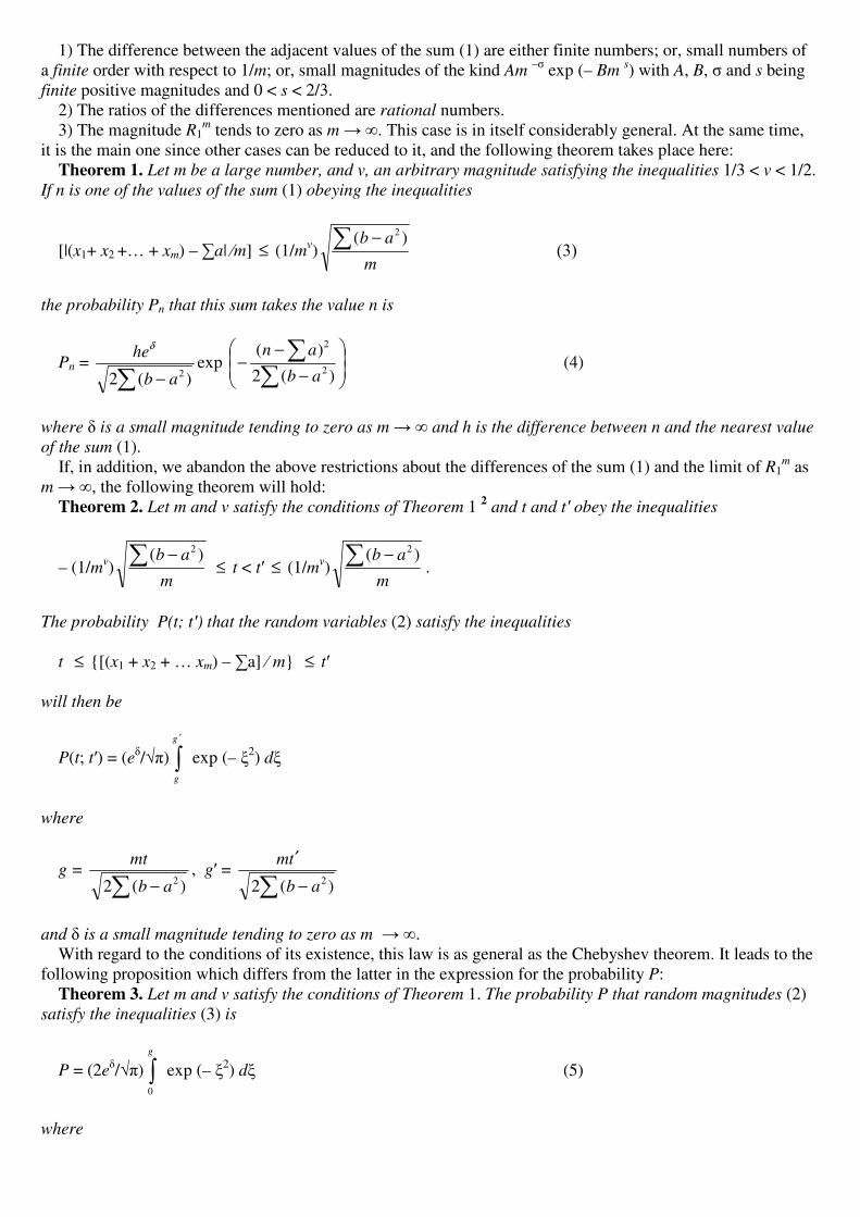
1) The difference between the adjacent values of the sum (1) are either finite numbers; or, small numbers of a finite order with respect to 1/m; or, small magnitudes of the kind Am

– exp (– Bm s) with A, B, and s being

finite positive magnitudes and 0 < s < 2/3. 2) The ratios of the differences mentioned are rational numbers. 3) The magnitude R1

m tends to zero as m � �. This case is in itself considerably general. At the same time, it is the main one since other cases can be reduced to it, and the following theorem takes place here: Theorem 1. Let m be a large number, and v, an arbitrary magnitude satisfying the inequalities 1/3 < v < 1/2. If n is one of the values of the sum (1) obeying the inequalities

[|(x1+ x2 +… + xm) – �a| �m] ≤ (1/mv)m

ab� − )( 2

� �

the probability Pn that this sum takes the value n is

Pn = � − )(2 2ab

heδ

exp ��

�

�

��

�

�

−

−−��

)(2

)(2

2

ab

an (4)

where � is a small magnitude tending to zero as m � � and h is the difference between n and the nearest value

of the sum (1). If, in addition, we abandon the above restrictions about the differences of the sum (1) and the limit of R1

m as m � �, the following theorem will hold: Theorem 2. Let m and v satisfy the conditions of Theorem 1 2 and t and t! obey the inequalities

– (1/mv)m

ab� − )( 2

≤ t < t� ≤ (1/mv)m

ab� − )( 2

.

The probability P(t; t!) that the random variables (2) satisfy the inequalities t ≤ {[(x1 + x2 + … xm) – �a] � m} ≤ t� will then be

P(t; t�) = (e�/��) �′g

g

exp (– �2) d�

where

g =

� − )(2 2ab

mt, g� =

� −

′

)(2 2ab

tm

and � is a small magnitude tending to zero as m � �. With regard to the conditions of its existence, this law is as general as the Chebyshev theorem. It leads to the following proposition which differs from the latter in the expression for the probability P: Theorem 3. Let m and v satisfy the conditions of Theorem 1. The probability P that random magnitudes (2) satisfy the inequalities (3) is

P = (2e�/��) �

g

0

exp (– �2) d� (5)

where

g = 2

21 vm

−

(6)

and � is a small magnitude tending to zero as m � �. Since g, as determined by (6), tends to infinity when m

increases, the probability P approaches 1. In the general case, the explicated conditions reveal a regularity in the deviations of the sum (1) from �a similar to the conformity, established for the phenomena considered by the Bernoulli theorem and for the mean values of observational errors. Under arbitrary circumstances, as formulated by the conditions of the abovementioned general theorems, this regularity seems unaccountable. Conformities in the cases of the Bernoulli theorem and of the observational errors are explained by the situation {?}, by the properties of the appropriate phenomena and the constancy of some conditions. With regard to such conformities Quetelet minutely develops the idea that they are occasioned by constant causes and by the mutual annihilation of perturbational effects3. However, his deep deliberations evidently do not concern mass independent phenomena studied under the general conditions formulated in the theorems above. These conditions allow any mutual relations between the causes occasioning independent phenomena. The problem of explaining the conformities taking place under such irregular conditions remains open. 3. More precise conclusions with regard to the probabilities of mass independent phenomena demand the introduction of a special supplementary variable r connected with n. Let us indicate first of all this connection. Suppose that �(r) = [�1(r)��2(r) … �m(r) r–n]1/m and let r be the positive root of the equation ��(r) = 0. Since this equation is reduced to r – 1 = tF(r), t = (n/m) – (�a/m) and n is given, the determination of r is not difficult. Evidently r can be expanded in powers of t by means of the Lagrange formula and the series will converge rapidly. We shall suppose that the expectations of the various powers of the variables (2) are such that the functions �i(e

), i = 1, 2, …, m

can be expanded into series in integral positive powers of convergent for ’s not greater by absolute value than some finite limit. Denote the modulus of the function �(re

i) by R. Its greatest maximal value over – � < < + � is obviously �(r). Imagine the other maxima of the function R not coinciding with �(r), and denote the greatest of them by R1. If, however, the function R has no other maxima excepting �(r), then we shall denote by R1 the minimal value 4 of R. Evidently, R1 < �(r). For the sake of simplicity we shall restrict our attention to the case in which {1/m lg[�(r)/ R1]} � 0 as m � � and the order of this small magnitude, taken with respect to 1/m, differs from zero by a finite magnitude 5. These conditions are supposed to be fulfilled in all the theorems below. In addition, everywhere below the differences between the adjacent values of the sum (1) are supposed to be either finite, or small magnitudes of an arbitrary finite order with respect to 1/m, and the ratios of these differences are rational. Theorem 4. The probability Pn that the sum (1) takes a given value n is

Pn = )(2

)]([ 2/1

rmr

rhm

ψπ

ψ

′′

+

(1 + �) (7)

where � is a small magnitude of an order not less than 1 with respect to 1/m and h takes the value indicated in

Theorem 1.

Formula (7) is applicable more widely than (4) and is more precise. The latter can, for example, lead to a false opinion that the most probable value of n is always equal to the value of (1) nearest to �a. The more precise formula (7) reveals, however, that under certain conditions the stipulated value of n can be separated from �a by a few intermediate values of the sum (1). Theorem 5. Suppose that Theorem 4 holds for all the values of n situated between �a – l and �a + l. If �1 and �2 are the values of

mr

−)](lg[ψ (8)

for n = �a � l respectively, then

P(| x1 + x2 + … + xm – �a | ≤ l) = (1/��) �−

2

1

ξ

ξ

exp (– �2) d� + � (9)

where � is a small magnitude of an order not lower than 1/2 with respect to 1/m. This theorem provides a more precise and a more widely applicable expression for the probability P than does Theorem 3. Theorems 4 and 5 have an additional feature in that they determine the order of smallness of the relevant errors. When applying formula (9) to the case of the Bernoulli theorem we must assume that �1(r) = �2(r) = … = �m(r) = q + pr where p is the probability of the occurrence of the {appropriate} event E and q = 1 – p. The probability P that the number n of the occurrences of the event in m trials will satisfy the inequalities | n – mp | ≤ l (10) is represented by formula (9) with �1,2 = {(mp � l) lg [1 � (l/mp)] + (mq ± l) lg [1± (l/mq)]}1/2. (11) This expression for P can easily be obtained in the usual way, that is, by means of the Stirling formula. It holds for all such values of l for which the absolute value of l/m remains less than the least of the numbers p and q. Thus, the expression for P is not only more precise, it also has a wider range of application as compared with the generally used formula (5) for the probability P considered in the Bernoulli theorem. Note also that the expressions for P defined by equations (9) and (11) easily provide the highest limit of the error �. 4. The precision of the approximate expressions for probabilities P and Pn can be raised still more. Denote the expectations of the cubes of the variables (2) by c1, c2, …, cm. Issuing from them and from formula (7), we arrive at Theorem 6. Let n� and n� be the least and the greatest values of the sum (1) for which the following

inequality holds | x1 + x2 + … + xm – �a | ≤ l. (12) Denote by �� and �� the corresponding values of the expression r2��(r)/ �(r), and, by u1 and u2, the

corresponding values of (8). The probability P that the random variables (2) obey inequality (12) is

P = (1/��) �−

2

1

u

u

exp (– �2) d� + m

u

2

)exp( 2

1

π

−[h/(2���) – B] –

m

u

2

)exp( 2

2

π

−{[h/(2���)] – B} + �

where h is the same as in Theorem 1,

B=�

�−

+−2/32

3

)]()/1[(6

)23()/1(

abm

aabcm

and � is a small magnitude whose order is not lower than 1 with respect to 1/m.

When applying this proposition to the case in which the conditions of the Bernoulli theorem are valid, we come to its following modification. Let p be the probability of phenomenon E and q = 1 – p. Denote the least and the greatest integers obeying the inequality (10) by n� and n� respectively, and set

u1 = ���

����

� ′−′ ′−′ nmn

mq

nm

mp

n)()(lg

with u2 differing from u1 in that n� is replaced by n�. Suppose also that the magnitudes (n�/m)[1 – (n�/m)] and (n"/m)[1 – (n�/m)] remain positive and do not tend to zero as m � �. Then the probability P that the expected number n of the occurrences of E in m trials satisfies inequalities (10) will be

P = (1/��) �−

2

1

u

u

exp (– �2) d� + m

u

2

)exp( 2

1

π

−���

����

� −+

′−′ pq

p

nmn

m

6

12

)(2–

m

u

2

)exp( 2

2

π

−���

����

� −+

′′−′′ pq

p

nmn

m

6

12

)(2 + �

where � is a small magnitude whose order is not lower than 1 with respect to 1/m. In concluding, we offer a more precise expression for Pn than the one provided by formula (7). Introduce

(z) = )(lg)](lg[

)1( 2

rrz

z

ψψ −

−,

then the last theorem follows: Theorem 7. The probability Pn that the sum (1) takes value n is

Pn =m

rhm

2

)]([

π

ψ���

����

�+

−+�

==

+s

k

zk

kk

kk

k

dz

zzd

km112

2/)12(2

2

2/1 ]})]()[/1{(

[!2

)1()]1([ δ

θθ (13)

where � is a small magnitude whose order is not lower than (s + 1) with respect to 1/m and h is the same as in

Theorem 1.

The right side of (13) is similar to the Stirling formula in that it becomes divergent at s = �. The following approximate value of Pn has no such peculiarity:

Pn = m

rhm

π

ψ )]([ ·

��

�

�

��

�

�+

−+−� �

==

+m s

k

zk

kk

k

k

k

dz

zzd

km

Jduu

τ

δθ

θ0 1

12

2/)12(222/1 ]

})]()[/1{([

)!2(

)1()exp()]1([ . (14)

Here

Jk = �mτ

0

exp (– u2)u2kdu

and � is a positive magnitude which is either finite or small, of order < 1/2 with respect to 1/m. This magnitude is not greater than the radius of convergence of the Lagrange series representing that root of the equation

z – 1 = ± i� )(zθ

which becomes 1 when � = 0. The number � in (14) is a small magnitude of order (s + 1) with respect to 1/m.

At s = � it will not be zero but a small magnitude having order + � with respect to 1/m. I shall present a detailed proof of all the results formulated above at a later date provided that circumstances will allow me to put my calculations in an order suitable for publication. 2 August 1898 Notes 1. {Nekrasov was introducing a new term, random magnitude, as it is still called in Russian, but he subsequently (see below) made use of other expressions as well which testifies that the new terminology was then not yet established. On this point see Sheynin (1996, §15.4).} 2. {Later on Nekrasov (1900 – 1902; 1900, p. 585, note 2) stated: “To the conditions of Theorem 2 it is necessary to add all those of Theorem 1”.} 3. {In general, Quetelet was notoriously careless.} 4. {Soloviev (1997, p. 16) noted that Nekrasov had later specified that, in this second instance, R1 was the greatest minimal value of R.} 5. Nekrasov’s symbol lg obviously stood for natural logarithms.} References Chebyshev, P.L. (1867), Des valeurs moyennes. Nekrasov, P.A. (1900 – 1902), New principles of the doctrine of probabilities of sums and mean values. Sheynin, O. (1996), Chuprov. Göttingen. Soloviev, A.D. (1997), Nekrasov and the central limit theorem.

On Markov’s Article {of 1899} and My Report {of 1898}

P.A. Nekrasov

Markov’s papers (1898; 1899) supplementing each other at the same time adjoin in the closest way my report (Nekrasov 1898) […] whose offprints I have sent out at the end of September 1898 to many Russian mathematicians including him. I ought to say, first of all, that this report is only an introduction to my accomplished work and contains a preliminary and, for that matter, briefest description of the results obtained. For the sake of conciseness I was compelled to indicate much only by a single stroke, and to omit even more, delaying the ascertaining of everything until the envisaged complete publication of these works of mine. In the report itself, I had declared my intention of presenting a detailed derivation of the expounded findings for the readers’ judgement. Since Markov says nothing at all about the adjoining of his papers with my previously published works1, I am compelled to indicate this myself. I venture to stress that the most important finding of Markov’s papers can be obtained by considering one of the conditions of my Theorem 1. To prove my point, I compare this latter with Markov’s conclusions. I adhere to my notation. […]The expectations of xk, xk

2, xk3, xk

4, … obey the condition that in the vicinity of = 0 the function �k( e

i) can always be expanded in a convergent series in integral positive powers of . Theorem 1 of my report can be expressed in the following way. Suppose that the ratios of the differences of

the sums

x1 + x2 + … + xm (1) are rational numbers and R1

m � 0 as m � �. If n is one of the values of (1) and the difference [(n/m) – �(a/m)] is small, then the probability Pn that the sum (1) takes the value n is approximately

Pn = � − )(2 2

abn

h exp (– �2), �2 =

��

−

−

)(2

)(2

2

ab

an

where h is the difference between n and the nearest value of (1). The proof of this theorem is available in my unpublished works. Its conditions being fulfilled, the following corollary concerning all the values of � located between g and g�,

g = � − )(2 2

ab

mt, g� =

� −

′

)(2 2ab

tm,

should take place:

(1/��) �′g

g

exp (– �2) d� � P(t ≤ {[(x1 + x2 + … + xm) – �a] � m} ≤ t�).

For a1 = a2 = … = am = 0 (2) this corollary coincides with one of the theorems in Chebyshev (1891) which is the subject of Markov’s papers. We also note that among the conditions of the theorem above and its just stated corollary is one special restriction lacking in Chebyshev (1891): lim R1

m = 0 as m � �. (3) Let us see whether condition (3) is always fulfilled when (2) holds and lim bk = 0 as k � �. (4) Now the expectation of xk

2 is bk = � pk xk

2 (5) and (4) and (5) lead to lim pk xk

2 = 0 as k � �. (6) Suppose that conditions lim pk xk

n = 0 for n = 3, 4, 5, … as k � � (7) also hold. Note that Markov’s example (Markov 1899) satisfies conditions (7). From (6) and (7) it follows that lim � pk xk

n = 0, n = 2, 3, 4, … as k � �. (8) In addition,

�k[e i]= 1 +

!1kiaθ

– !2

2kbθ

+ … + !n

xpin

kk

nn �θ + … (9)

and if (3) is valid

�k[e i]= 1 –

!2

2kbθ

+ … + !n

xpin

kk

nn �θ + … (10)

Taking into account (5), (8) and (10), we have 2 lim �k[exp(1i)] = 1 as k � �. At the same time the expression {f [exp(1i)]}

m = �1[exp(1i)] �2[exp(1i)] … �m[exp(1i)] can have at m = � a finite limit differing from zero and, as shown by its definition, R1

m will not vanish as m = �; that is, condition (2) of Theorem 1 of my report will not be fulfilled. Thus, it can fail if (3) and (4) are valid. On the contrary, if equality (4), given condition (3), does not hold, i.e., if bk does not tend to zero as k � �, then equality (10) will not be valid either, and, instead of it, we will have the inequality lim �k[exp(1i)] < 1. k � � In this case, condition (3) and, along with it, Theorem 1 of my report and its corollary represented by the abovementioned Chebyshev theorem must be completely valid. It is this latter conclusion which follows from

condition (2) of my report and which constitutes the essence of those inferences made by Markov (1898) and formulated by him as a special additional (third) condition of the Chebyshev theorem: the expectation of xk

2

does not become infinitely small as k increases infinitely. The same conclusion is contained in Markov (1899), only it is there expressed in other words and illustrated by the abovementioned example for which conditions (8) take place. Indeed, the Chebyshev theorem under consideration does not here hold. Since Chebyshev does not include Markov’s condition, then, obviously, Markov claims it for himself. It should also be noted that, had Chebyshev himself noticed the insufficiency of the restrictions of his theorem, he would have probably supplemented his theorem in a more satisfactory manner. I am again led to this assumption by the abovementioned comparison of Markov’s additional condition with the restrictions of Theorem 1 of my report. It follows from this comparison, that Markov’s additional condition, being a corollary of my condition (3), at the same time worsens it in the sense of comprehensiveness. Indeed, this condition does not include many cases in which the theorem of the Chebyshev memoir is valid. In other words, in its Markovian form, it can remain unfulfilled: the expectation of xk

2 can tend to zero whereas restriction (2) of

Theorem 1 of my report can still be obeyed and its corollary, i.e., the abovementioned theorem from the Chebyshev memoir, will certainly hold. In concluding, I consider it appropriate to answer here to the reproaches, made by a critic in connection with my report, and related to the subject of this article. First, I touch on the reproof that I, having devoted my report to the memory of Chebyshev, allegedly forgot his memoir (1891). It should be stated that I had not forgotten the domain with which this memoir has to do, that is, the doctrine of the mean values of observational errors. I called this doctrine well-known, but I did not list the appropriate memoirs of Laplace, Chebyshev or others because of the conciseness of my account rather than of forgetfulness. And I had no grounds for separating the Chebyshev memoir from the other sources also because I am arriving at my conclusions not by his methods, but by different ones, which in this instance I consider more fruitful. My methods are based on approximately calculating functions of large numbers by means, which were initially expounded in an imperfect but deeply conceived form by Laplace, and then developed by Cauchy, Darboux and others. I have touched on these methods in a work (1885) whose unpublished chapter includes their improved version and represents a most essential part of my investigations. These methods enjoy an important advantage. Not only do they provide the limiting expressions of the probabilities treated in the Chebyshev memoir (1891), they also open up special

means for estimating the boundaries of their errors. The power of these methods in the indicated sense is evident from their particular application to the Bernoulli theorem. I have isolated this point from my unpublished works and put out an appropriate paper (1899)2. Finally, it is yet necessary to note also that the abovementioned Chebyshev theorem only pays attention to the sum of the probabilities which is sufficient for establishing the method of least squares. Such a restriction does not however satisfy those who bear in mind the entire field of applications of the theory of probability including statistics. These applications require the knowledge not only of the sum (or the integral), but also of each summand (or differential). When studying curves, it is important to know not only their lengths, but also

all of their windings characterized by their differential properties; so also, when studying mass phenomena with which statistics is dealing, it is important to have a notion about the probability of any combination of these chances random occurrences. Second, I shall answer the reproof concerning Theorem 2 of my report which is expressed insufficiently clearly or fully. I find this criticism partly just and explain the shortcomings of the theorem by my striving for conciseness as well as by the fact that Theorems 1 and 4 were in my opinion the most important ones, whereas Theorem 2 was formulated in passing. I asked my critic to pay attention mostly to those principal theorems which I had advanced to the forefront in the appropriate sections of my report. I shall also add that, undoubtedly, after a complete publication of my works and the ascertaining of all my methods, the shortcomings in the expression of Theorem 2 will be overcome. Notes 1. {I believe that the only relevant published works were Nekrasov (1898; 1899).} 2. {As nekrasov explained in the beginning of his paper, here omitted, 1 corresponded to R1 = mod{f [exp(1i]]}.}

3. I have, for example, found out the precision of the approximate value of the probability P that, after tossing a coin 20 000 times, there will be not less than 9800, and not more than 10 200 heads: P = 0.995 330 with an error less than 0.0001 in absolute value. No-one had until now possessed a method of providing such results, and Chebyshev’s memoir does not furnish them. References Chebyshev, P.L. (1891), Sur deux théorèmes relatifs aux probabilités. Markov, A.A. (1898), Sur les racines de l’équation … --- (1899), The law of large numbers and the method of least squares. Nekrasov, P.A. (1885), The Lagrange series, etc. --- (1898), The general properties of mass independent phenomena etc. Translated in this book. --- (1899), The boundaries of the errors of the approximate expressions of the probability, etc.

An Answer

A.A. Markov The lines below represent a brief answer to an interesting note of Nekrasov (1899). My articles (1898; 1899) contain a rigorous proof of the well-known theorem on the limit of probability. Its demonstration is connected with ascertaining some properties of the roots of the equation exp (x2)�{d

m[exp(–x2)] � d x

m}= 0. As to Nekrasov’s report (1898), it is an unsubstantiated declaration about new theorems, or about such propositions which he thought fit to consider new. Not only are there no hints of the properties of these roots, or of a rigorous proof of the abovementioned theorem on the limit of probability; even its correct formulation is lacking. I borrowed the formulation of the theorem not from Nekrasov, but from Chebyshev’s memoir (1891), which Nekrasov, who had unfoundedly devoted his report to Chebyshev’s memory, did not consider it necessary to mention. To the conditions explicitly stated by Chebyshev I have added one more, not calling it new because of Poisson’s example (1824) which I mentioned. Nekrasov has no claim to this condition, and his reasoning, by whose means he tries to create this claim, is not supported by evidence and mistaken. Such a reasoning does not deserve a detailed analysis. One example will suffice to prove his mistake and, at the same time, to ascertain, once and for all, the groundlessness of Nekrasov’s pretensions. Let xk take values 1, – 1, 1/2k and – 1/2k with probabilities (1 – p)/2, (1 – p)/2, p/2 and p/2, respectively. Here, p does not depend on k and is less than 1/2. Then, in Nekrasov’s notation, ak = 0, bk = 1 – p + p/22k, lim bk = 1 – p > 0, k # $

The inequality reveals that the condition, which I added, is fulfilled. It is not difficult either to see that, in this case, all the other conditions of the theorem on the limit of probability formulated by Chebyshev are also obeyed. Turning now to Rm, we note that in our example this magnitude is equal to the absolute value of the product [(1 – p)cos + pcos(/2)]�[(1 – p)cos + pcos(/22)] … [(1 – p)cos + pcos(/2m)] and attains one of its maximal values, (1 – 2p), at = 2m�. Therefore, R1

m ≥ 1 – 2p and cannot tend to zero as m # $. In other words, Nekrasov’s condition (2) remains unfulfilled. So, contrary to his assurances, all the restrictions of the theorem on the limit of probability, both ascertained by Chebyshev and added by me, can be fulfilled in such cases also in which Nekrasov’s condition (2) does not hold. References

Chebyshev, P.L. (1891), Sur deux théorèmes relatifs aux probabilités. Markov, A.A. (1898), Sur les racines de l’équation … --- (1899), The law of large numbers and the method of least squares. Nekrasov, P.A. (1898), The general properties of mass independent phenomena, etc. Translated in this book. --- (1899), The boundaries of the errors of the approximate expressions, etc. Poisson, S.D. (1824), Sur la probabilité des résultats moyens des observations. Conn. temps pour 1827, pp. 273 – 302.

On Academician Markov’s “Answer”

P.A. Nekrasov

1. I (1898) introduced a special additional condition into Theorems 1 and 4 – 7 on the probabilities of mass independent phenomena. It did not occur in the writings of my predecessors, and it is connected with the properties of a special magnitude, R1. Later on, Markov had offered his own additional condition, which, as I (1899a) showed, followed from my condition as a particular corollary and unnecessarily restricted the theorem {which one?}. In his “Answer” (1899b) Markov attributes his additional condition, which he also put forward earlier (1898), to Poisson. The latter, however, had not derived it in the place indicated by Markov in such a restrictive form. 2. In the same “Answer” Markov refutes my additional condition. To this end, he offers an “example” which he considers sufficient “to ascertain, once and for all, the groundlessness of Nekrasov’s pretensions”. However, his illustration obviously does not achieve its goal. The misunderstanding consists in that Markov inappropriately defined the magnitude R1 which plays an essential role in my additional condition. Indeed, in my memoir (1898) this magnitude is applied in Theorem 1, and is defined as one of the minimal values of the modulus R of function f [e i] which do not coincide with 1. It follows that the maximal values coinciding with 1 are here eliminated. These eliminations ought to take place for very large values of m, and, obviously, also in the limit, when m = �. Markov, however, in spite of the indicated definition of R1, chose it from among the maximal values of R in such a way that it obeys the inequalities (1 – 2p)1/m ≤ R1

< 1 and therefore coincides

with 1 when m = �. His considerations, based on such an inappropriate definition of R, do not deserve any attention. 3. In his “Answer” Markov reproaches me with unsubstantiating my report. This, however, is of no consequence since I have stated that the proofs, which I possess, will be offered in the near future. Given such a statement, it would have been necessary to wait for these demonstrations and then to look into the matter rather than to engage in hasty fault-finding with respect to a semi-published work which as yet had received so to say only a detailed title in my memoir (1898). The Academician is possibly displeased at some delay in the appearance of these proofs. But this is occurring through no fault of mine, it depends on the fact that the material in my possession is too voluminous.

The business will not suffer from such a delay, it will only benefit from it because the proofs will be deep and thorough rather than shallow and premature. Their exposition demands an entire treatise at whose composition I am honestly toiling for many years now. And it is necessary, above all, to revise and reconstruct there the concepts and methods connected with approximately calculating the integrals of the type

� f (z)�m(z) dz (1)

and to apply the thus perfected calculus to probability theory. The first and the most essential half of this treatise will appear in vol. 21 of the Matematichesky Sbornik as “Calculus …” (1900). Its offprints are already published and sent to many mathematicians on October 15, 1899. (According to the printing-houses’ custom, they are dated 1900.) The other part which will bear on the application of this calculus to probability proper, and in particular will include the proof of the results explicated in the memoir (1898), is to appear later on. However, having been undeservedly reproached with the lack of substantiation just when I am saying and doing everything possible to acquaint the scientific community with the demonstrations, I am compelled to say something right now about them […] The “Calculus…” is already sufficient for convincing skeptical readers that the proof of my results (1898) is quite possible. Indeed, the probability Pn is represented there, in §3 (n°7), by an integral of the type (1) so that the problem is reduced to the methods {?} indicated in the “Calculus…”. In addition, in §11 (n° 37) it is established that in a certain main case the determination of Pn is reduced to calculating a far term of a

Lagrange series, and in n° 38 of the same section the method itself of obtaining approximate expressions of such terms is ascertained in sufficient detail. Given these indications, those who so desire can easily derive the proofs of the theorems of my memoir (1898). To recall, I have already busied myself with the problem of approximately calculating the terms of the Lagrange series in my article (1885). It follows that I possess these proofs for about 15 years which is sufficient for penetrating all the appropriate fine points to a depth hardly attainable for Markov since he was not interested in such investigations to the same extent. A new magnitude plays an essential part in the methods of calculating integrals of type (1) and of the far terms of the Lagrange series. In the “Calculus…”, it is denoted by K2 and defined according to a rule explicated in §6 (n° 21). It is important both when estimating the errors of approximate expressions and for deriving the conditions of their suitability or unsuitability. In (1898), this magnitude, which occurs when calculating the probability Pn by the methods indicated, is denoted by R1 . It is included in the expression for the abovementioned additional condition of Theorems 1 and 4 – 7. The origin and the meaning of this restriction, with which Markov has such strange relations, and which is the result of a thorough and deep study rather than of a shallow and hasty conclusion, is thus completely explained. In §6 (n° 21) of the “Calculus…” I also interpret such special cases of defining K2 to which the “example” of the Academician belongs and which are connected with the new concept of sub-principal points. In my subsequent writing I shall show that, other conditions being given, my additional restriction is sufficient and at the same time almost necessary. As follows from the same work, for transforming it into a sufficient and quite necessary criterion some (insignificant) complication is needed. I had not introduced it in (1898) for the sake of simplicity. 4. The application of the “Calculus…” also eliminates the unnecessary restrictions in the other conditions of the theorems on the probabilities of mass random phenomena and thus leads to rigorously proved laws of these phenomena in the most general form. Such a form of these laws is close to the one briefly formulated in (1898, Theorems 4 – 7); it will be more fully developed in my subsequent writing. Let us compare this form of the abovementioned laws with their previous expressions taking account of expectations. All previous authors including Chebyshev (1891) restricted expectations not in accord with the essence of the matter, but due to the imperfection of derivation. These restrictions concerned the expectations of the powers of random variables x1, x2, …, xm and demanded that the expectations of xk

n as n # $ be finite. However, for the validity of Theorems 4 and 7 (1898), from which all the other propositions there included follow, the expectations should obey a less significant restriction consisting only in that each function �k (e

z) = � pk exp (z xk)

where k = 1, 2, …, m be holomorphic in the domain of point z = 0. It follows that for large values of n the

expectation of xkn can be very large and even infinite when, in the limit, n = �. Under this condition Theorem 4

and its corollary remain fully valid if only, together with the holomorphy of the functions �k(ez), the

abovementioned (§§1 and 3) additional condition persists. The possibility of eliminating such unnecessary restrictions is implicit, in general, in the peculiar properties of my methods, which, wherever they might be applied, can always lead to the most precise expressions of the conditions, i.e., to conditions not only sufficient but at the same time necessary. Thus, in the problem similar to the calculation of the probability Pn and concerning the errors of interpolation formulas, my methods lead to a new form of the condition of suitability 1 which occur to be not only sufficient but also necessary (“Calculus…, §13). Having mentioned Chebyshev, to whom report (1898) is dedicated, I shall say that, from among his writings devoted to expressing the general laws of mass random phenomena, I set infinitely high store by his immortal memoir (1867) which is a greatest contribution to science. And I consider his memoir (1891) as of minor

importance since it contains that, which was sufficiently rigorously proved much earlier and included in generally known treatises (Laurent 1873, pp. 144 – 165) 2. It is interesting only as being one of the successful applications of Chebyshev’s great inventions to earlier exhausted problems. Returning to my method of investigating probabilities of mass phenomena based on the “Calculus…”, I shall add that it is inferior to other methods of the same kind, which provide only sufficient conditions, solely in that it is based on more involved reasoning. Properly speaking, however, this complexity is not a shortcoming of the method since more precise conditions, i.e., such as are not only sufficient but also necessary, always demand more complicated reasoning for their derivation. In this case, the complexity only testifies that my method is on the summit of knowledge rather than in its lower layers. 5. While reproaching my memoir (1898), Markov, not without success, enjoys its fruit as well as that of its particular supplement (Nekrasov 1899b). I do not understand the first (i.e., the reproach), but I can only sympathize with the second if only the man who is enjoying himself does not forget to mention his predecessor who gave the fruit to him. Among the most important features of my memoir (1898) I should point out the new forms of the approximate expression of the probability Pn indicated in Theorems 4 and 7. These forms are distinguished by higher precision as compared with the old (Laplacean) form of Pn applied in Theorem 1. And the advantages of the new form are sufficiently explained there. When applied to the Bernoulli theorem, it turns into the well-known form derived from the Stirling formula which previous calculators were corrupting by excessively transforming it into the Laplacean form. I (1898) have indicated benefits of another kind, of the kind more fully realized in (1899b). There, I had absolutely banished from use the Laplacean form of the approximate expression of Pn, and, to the great advantage of the subject at hand, applied the form corresponding to Theorems 4 and 5. Later on Markov (1899a) made use of this fruitful idea and successfully combined it with a helpful, in this case, application of continuous fractions. 6. I must repeat and supplement here my statement made at the end of (1899a) about a necessary correction. My additional condition (§§1 and 3), whose expression is connected with the magnitude R1 (1898, Theorems 1 and 4 – 7), should also be made with respect to Theorem 2 of the same memoir. That I have overlooked (in Theorem 2) this condition, which runs all through the memoir, is what is called lapsus calami {slip of the pen}. This mistake can at least be partly explained by my excessive trust in my celebrated predecessors such as Laplace, Chebyshev, et al. My lapse is however easily noticeable since it was made not in the main Theorem 1, but in its corollary, in Theorem 2. Notes 1. Incidentally, Markov (1889 – 1891) overlooked the well-known conditions of suitability of interpolation formulas and mechanical squaring. 2. {This statement is strange indeed. And the correct pages in Laurent (1873) are 144 – 145 which in itself almost refutes Nekrasov who repeatedly underrated Chebyshev’s proof of the central limit theorem. Thus, in a letter of 30 Oct. 1915 to Andreev (Chirikov & Sheynin 1994, p. 157 of translation), Nekrasov declared that it was not a theorem in the strict sense but a postulate correct until finite

magnitudes of probability are discussed, but having numerous exceptions

otherwise.

Elsewhere Nekrasov (1916, p. 54) strangely defined postulate as a rule spoiled by exceptions.}

References Chebyshev, P.L. (1867), Des valeurs moyennes. --- (1891), Sur deux théorèmes relatifs aux probabilités. Laurent, H. (1873), Traité du calcul des probabilités. Paris. Markov, A.A. (1889 – 1891), ���������� � ������ ���� ��� (Calculus of Finite Differences). --- (1898), Sur les racines de l’équation … ---(1899a), Applications of continuous fractions to calculating probabilities. ---(1899b), An answer. Translated in this book. Nekrasov, P.A. (1885), The Lagrange series etc. --- (1898), The general properties of mass independent phenomena etc. Translated in this book. --- (1899a), On Markov’s article […] and my report […]. Translated in this book. --- (1899b), The boundaries of the errors, etc. --- (1900), Calculus of approximate expressions, etc.

Concerning a Simplest Theorem on Probabilities of Sums and Means

P.A. Nekrasov 1. My research (1900 – 1902) contains critical historical remarks which fully ascertain the shortcomings of the results both of Chebyshev’s memoir (1891) and of the attempts of Academician Markov to supplement its main theorem and to make its deduction more rigorous. At the same time as my investigation appeared, Prof. Liapunov published two papers (1900; 1901) where he tried to eliminate some restrictive conditions, whose uselessness I had previously indicated, of the theorem in the Chebyshev memoir, and to substantiate his deductions more rigorously. Regrettably, having applied to this end the Dirichlet discontinuity factor, Liapunov overlooked the well-known difficulties encountered in applying it in his case 1. And he obtained results containing all the main shortcomings of the conclusions of his predecessors minutely treated in my abovementioned investigation. Thus, Liapunov utterly overlooks that the Laplacean approximate expression for probability, which he is using, can hold only in a restricted domain indicated in my memoir (Ibidem, nn° 36 – 37). Then, special cases of the first kind adjacent to the normal cases 2 are possible if special restrictions are not imposed on the limits of integration. The application of formulas of the Laplacean type even in the mentioned curtailed domain is not possible here. The correctness of these objections is easily confirmed even by elementary considerations. The first one is substantiated by means of the elementary principle of duality (Ibidem, nn° 24 – 27) and the second one is easily justified by simple examples in which the theorem leads to contradictions and I considered such an illustration (Ibidem, nn° 52 and 55). 2. In his memoirs, Prof. Liapunov attempted, for one thing, to combine the most general expression of the theorem on the probability of sums with an elementary expression of the conditions of this theorem. But it might be said that, in general, all such attempts are doomed to prove unsuccessful. The point is that an elementary expression of these conditions cannot be combined with a too wide generality of the problem to which the authors wish to apply the theorem. This incompatibility is clearly perceived in the expressions for the conditions of the normal case given in my memoir (Ibidem). In general, these conditions are extremely involved, and, in order to master them in full, we had to give them several expressions, calling them primary, secondary, tertiary, etc. indications. This breakdown of the expressions for the conditions of the normal case is similar to that which occurs in the theory of convergence of series with positive terms. However, it is even more complicated because the conditions of the problems on the probability of sums are much more general. It should be said that Chebyshev (1891), who had considered only the case in which the variables and their probabilities varied continuously, was less deviating from the truth than Markov, who eliminated this restriction, or Liapunov, who went even further in such a generalization of the conditions which is

irreconcilable with their elementary expression.

3. When desiring to obtain a theorem on the probabilities of sums and mean values so that its conditions are without fail expressed in an elementary way, we must restrict our data in some expedient manner. Let us try now to fulfil this work by means of our methods of research and to obtain thus the theorem of the Chebyshev memoir in a corrected form. This form, with its conditions expressed in an elementary way, will be of great interest since it is still wide enough to meet most practical demands. In keeping with the notation of my memoir (1900 – 1902), let �1, �2, …, �m (1) be m real variables whose values are determined by random independent events peculiar to m independent processes of observation respectively. Suppose that these variables are reducible; that is, represented as �i = �i + hxi, i = 1, 2, …, m, where xi are variable integers and h and �i are constants with h being chosen in such a way that the greatest common divisor of all the possible values of the sum x1 + x2 + … + xm is unity.We shall denote the probabilities pi of the variables (1) 3 in another way as p1(�1)h, p2(�2)h, …, pm(�m)h. (2) Suppose now that

k(u) = � pk(�k)h kkuγε −

(3)

where k is some number from among 1, 2, .., m and the sum is extended over all possible values of �k. Let us also say that the variation of the probability pk(�k)h, considered as a function of its argument �k, is regular if the values of �k constitute an arithmetic progression with common difference h, and if, in addition, for any values of �k lesser than its maximal value the ratio pk(�k+ h) to pk(�k) remains constant and does not vanish or become very small. Otherwise, we shall call the variations of this probability irregular. The case in which the probabilities of all the variables (1) vary regularly is remarkable as being important in the practical sense. When dealing with the probabilities of sums and mean values, we very often encounter exactly this case. Incidentally, it will take place if all the variables (1) are continuous and, at the same time, all the functions pk(�k) are finite and continuous, i.e., if the variations of the probabilities of all these variables be regular. If these variations are regular, then, at no integral value of µ > 1, the expressions of the type k(z�

w) – k(zw) (3�)

can not be, all together, very small. Here, � is any number from among 1, 2, …, µ – 1; k(u) is defined by equality (3), w = 1/h, z is an arbitrary number having modulus 1, and z� = ze

2� � i/µ. It follows then that, if the probabilities of all the variables vary regularly, the special case of the first kind

cannot occur. The case can be normal, or paradoxical, or special, but of the second kind. This elimination of the special cases of the first kind much simplifies the expressions of the appropriate theorems, which, generally, become complicated most of all because of these cases. If desirable, we can still widen the concept of regular variations of the probabilities pk(�k)h and call them regular if there does not exist any integral number µ (µ > 1) such that all the expressions of the type (3�) become zeros or very small. If the probabilities of all the variables (1) vary regularly in this more general sense, then under these conditions the special case of the first kind cannot take place either, so that the expressions of the appropriate theorems can be simplified.

Below, we shall suppose that the variations of the probabilities of all the �i’s are regular both for finite values of m and for its infinite increase. Denoting 4 E�k = ak1, E�

2k = ak2,

g = (1/m) [(a12 – a112) + (a22 – a21

2) + … + (am2 – am12)] (4)

we shall supplement the properties of g and h which have an important role in my memoir (1900 – 1902) by one remark. It is connected with transforming the variables (1) by means of equations �1� = ��1, �2� = ��2, …, �m� = ��m, (5) where � is constant. The new variables �i� (6) are represented as �k� = ��k + h�xk , k = 1, 2, …, m, h� = �h (7) and they are therefore reducible. Now, the expectations of �k� and (�k�)

2 will be a�k1 = �ak1, a�k2 = �2

ak2 and g! = (1/m) [(a!12 – a!11

2) + (a!22 – a!212) + … + (a!m2 – a!m1

2)], g! = �2

g (8) where g is defined by equality (4). Thus, the transformation of the variables by means of equalities (5) leads to the replacement of g and h by g! and h! defined by equations (8) and (7) respectively and by an arbitrary magnitude �. But then, having at our disposal this magnitude, we may demand that g! takes some positive value assigned beforehand. We shall call the variables �i� normal if this value is finite and does not tend to zero. If g! is given beforehand, we have from

equality (8) � = gg /′ . At the same time equality (7) will become h! = h gg /′ .

Transformation (5) allows us to avoid some more difficulties. When formulating theorems on the probabilities of sums, the case in which the variables (1) are not normal presents difficulties. However, these are easily eliminated since the indicated transformation of the variables allows us, without losing generality of the solution of problems, to consider only normal variables (1) and to eliminate the need to deal with the case in which g is either very large or very small. In Nekrasov (1900 – 1902, nn° 4 and 7) this case is considered as a paradoxical and sometimes as an instance bordering on the paradoxical. Thus, without loss of generality we may suppose that the variables (1) are normal so that g does not tend

either to zero or infinity. The most important corollary of this supposition and of the abovementioned assumptions on the variations of the probabilities of the variables (1) is that the magnitudes R1 and �(r) (Ibidem, n° 13) cannot be equivalent; their ratio cannot tend to 1 as m ��. Under these circumstances, the success of the further deductions depends only on the fulfillment of the restrictive conditions indicated in nn° 4 and 7 of the same memoir. Let them also be fulfilled. This happens if, for example, h does not exceed some finite boundary and, moreover, if the functions 1(u), 2(u), …, m(u) (9) determined by equations of the type (3) have no singular points excepting u = 0 and u = �. At the same time, if h pertains to the first kind, then we may apply Theorem 2 (Nekrasov 1900 – 1902, n° 13). If, however, it belongs to the second kind, or is too small, then we may make use of the methods of nn° 48 and 49. After that, we may follow the appropriate indications of nn° 19, 20, 46 and 36 where the conclusions

are formulated as theorems whose conditions are expressed in an elementary way. As a result of applying this, we obtain theorems whose conditions are formulated in an elementary way For example, we may state this proposition: Theorem. Let random variables (1) with either a finite or an infinitely increasing m be reducible, and,

moreover, normal. Suppose also that the variations of the probabilities (2) are regular and that the functions (9) have no singular points excepting u = 0 and u = �. Suppose then that h does not exceed a finite boundary

and that z1 and z2 satisfy the inequalities

m

gz

m

g 21≤−ν

< νm

g

m

gz≤

22 , (10)

v > 1/3. (11)

If z1 mg2 and z2 mg2 are such values of the sum

(�1 – a11) + (�2 – a21) + … + (�m – am1)

that (z2 – z1) mg2 exceeds h and is not less than a given small magnitude of a finite order with respect to 1/m,

then the probability P of the inequalities 5

z1 mg2 ≤ (�1 – a11) + (�2 – a21) + … + (�m – am1) < z2 mg2 (12)

being satisfied is equivalent to

(1/��) �2

1

z

z

exp (– z2)dz; (13)

that is,

(1/P��) �2

1

z

z

exp (– z2)dz � 1 as m � �.

If the variables (1) are here continuous, this theorem will turn into the main proposition of Chebyshev’s memoir (1891), modified, however, in such a manner that all its inaccuracies indicated by me (1898) are completely eliminated. The condition of the theorem above that demands that the variations of the probabilities of all the variables (1) be regular, protects us against those mistakes made by Markov and Liapunov which result from ignoring the special cases of the first kind. We have first indicated the conditions of our theorem presented by inequalities (10) and (11) in our report (1898). They also prevent us from mistakes of another kind. Chebyshev, Markov, Liapunov and other authors overlooked these conditions that play an essential role when applying formulas of the Laplacean type for calculating probabilities of sums (Nekrasov 1900 – 1902, nn° 36 and 37). When calculating the approximate expression for the probability P of inequalities (12) without introducing conditions (10) and (11) it is necessary, in general, to apply new formulas rather than those of the Laplacean type. Thus, bearing in mind the remarks (Ibidem, n° 33) and denoting

�k(u) =�kε

pk (�k) h kuε , F(u) = �1(u) �2(u) … �m(u),

it is easy to satisfy ourselves that the probability P of the inequalities (12) being obeyed is equivalent to

(1/��) �2

1

ξ

ξ

exp (– z2) dz

where

�1 = ± )](/lg[ 111 uFu

α , �2 = ± )](/lg[ 222 uFu

α ,

�1(u1 – 1) > 0, �2(u2 – 1) > 0. Then,

�1 = z1 mg2 + a11 + a21 + … + am1, �2 = z2 mg2 + a11 + a21 + … + am1

and u1 and u2 are the positive roots u of the equations

�1,2 = )(

)(...

)(

)(

)(

)(

2

2

1

1

u

uu

u

uu

u

uu

m

m

ϕ

ϕ

ϕ

ϕ

ϕ

ϕ ′++

′+

′

repectively. It is also necessary, however, that either 1 is located between the roots u1 and u2 or situated very close to one of them, and that under the change from �1 to �2 the sum n = �1 + �2 + … + �m (i) does not go beyond the domain (n) indicated by me (1900 – 1902, nn° 4 and 7). These conditions, that replace (10) and (11), are much wider than the latter ones and exclude only such domains of the variation of the sum (i) which are located partly close to either its minimal or maximal value. 4. The essence of the inaccuracies of the Chebyshev’s memoir (1891) and of the related investigations of Markov and Liapunov should also be further explained. The additional elucidation will make it clearer why these inaccuracies have escaped their attention. The conclusions of the abovementioned authors determine, under certain conditions, the limit of the probability P of inequalities (12). According to their opinion, this limit is always an integral of the type (13). But how should we understand here the term limit? In my investigations, and in the theorem above, I connect this notion with the concept of equivalence of the probability P and the magnitude L to which P tends: P and its limit L should be equivalent; that is, the ratio L/P should tend to 1. The same understanding of the term limit permeates also the entire analysis of infinitesimals, i.e., the differential and the integral calculuses. Only this understanding of the word limit I consider fruitful and quite deserving a rigorous scientific investigation. However, the conclusions of the abovementioned authors very often differ from this understanding. For them to become formally correct, another, more crude concept of limit is needed, a concept that is satisfied by keeping to one single demand that the difference (P – L) tends to zero. Here, P and L can be non-equivalent in the above sense if they themselves tend to zero. Assuming such a crude understanding of limit, any magnitude of the type x

n with n > 0 can, for example, be considered the limit of sin x as the absolute value of the arc x tends to zero. It should be said that the conclusions of the abovementioned authors never differ from such a concept of limit. However, many extremely important problems do not reconcile themselves to such crude notions or to calculations based on them. Take for example the practical problem about the insolvency of a bank having a given money fund A and obliged to pay out random sums �1, �2, …, �m. If this bank is reliable, the probability of its insolvency, i.e., of the inequality A < �1 + �2 + …, �m, is very low. To know this probability at least approximately is extremely interesting. Our conclusions, and especially those which are connected with the new formulas, provide a means to determine very precisely the magnitude L equivalent to P. At the same time, under the same conditions, the conclusions of the abovementioned authors very often provide expressions non-equivalent to this very low probability P since the conditions (10) and (11) are violated. These expressions cannot be considered practically valuable; sometimes they can even mislead. The authors could have avoided such delusions by issuing from our more rigorous notion of limit and more carefully applying the means of calculation at their disposal. Thus, it was possible, taking adequate precautions, to make use also of the Dirichlet discontinuity factor. (I, however, would have preferred other such factors with finite limits of integration.) It would have then been necessary to check not only that the difference (P – L) is small and tends to zero, but also that the order of this small magnitude is higher than the order of L. In cases in

which P is very low the authors very often violate this latter demand. Had they, however, preferred to avoid this

violation, they should have followed our advice (1900 – 1902, n° 60) according to which not only the main point of the basic path of integration should be considered, but all the principal, and sometimes even the sub-principal points. We shall devote a special investigation to such more careful applications of discontinuity factors to the doctrine of probabilities of sums and mean values. 12 (25) March 1901 Notes 1. These hindrances are partly ascertained in Markov’s treatise (1900), but the main difficulty is indicated in my historical remarks (1900 – 1902). {Nekrasov (Ibidem, 1901, p. 110) specified his reference to Markov by indicating the page numbers (1900, pp. 80 – 88).} 2. {At the time, the term normal law or normal distribution was not yet generally used so that Nekrasov (either here or below) should not be blamed for introducing confusion.} 3. {Probability of variable: unfortunate expression.} 4. {Notation of the type EX is my own.} References Chebyshev, P.L. (1891), Sur deux théorèmes relatifs aux probabilités. Liapunov, A.M. (1900), Sur une proposition de la théorie des probabilités. --- (1901), Sur une théorème du calcul des probabilités. Markov, A.A. (1900), ���������� ��� �� ��� (Calculus of probability). Nekrasov, P.A. (1898), The general properties of mass independent phenomena, etc. --- (1900 – 1902), New principles of the doctrine of probabilities, etc.

An Answer to P.A. Nekrasov

A.M. Liapunov

Foreword by Translator

In 1901 Nekrasov wrote a letter to Liapunov which contained the following lines (Tsykalo 1988, p. 84):

According to my profound conviction, your theorems, as well as

Chebyshev’s propositions, contain errors. […] And if, in addition,

you generalize these theorems in the same direction, the errors will

intensify. […] Why are you in such a hurry to publish papers on

problems which are very new for you, and in which so many subtle

complications, escaping notice at first sight, present themselves? Two weeks later, in a letter to Steklov (Nauchnoe 1991, p. 25) Liapunov mentioned Nekrasov’s impudence. Similar strong words are in Liapunov’s letter of 29 March of the same year to the mathematician Konstantin Alekseevich Andreev, 1848 - 1921 (Sheynin 1989, p. 307). And in a letter of 21 April Liapunov thanks Andreev for advising him to extend the initial manuscript of his Answer. The last section (§9) of this contribution seems to be very interesting; apparently, no-one paid due attention to it. * * * 1. Nekrasov’s just appeared article (1901) includes a number of attacks on my papers (1900; 1901). He declares that these contain mistakes and that my findings are corrupted by all the main shortcomings of the results of my predecessors (that is, of Chebyshev and Markov, whose contributions also come under Nekrasov’s assault). Nekrasov allegedly ascertained these imperfections in full in his recently published work (1900 – 1902) 1. Nekrasov, however, only corroborates his statement by very indefinite general reasoning from which nothing can be concluded, and cites his own work just mentioned above. In spite of his opinion, he did not reveal there any deficiencies in Chebyshev’s or Markov’s works. If the reference to his work aimed at indicating a discrepancy between my conclusions and his, then it was absolutely superfluous. I do not at all deny the disagreement, which, however, can hardly be considered as a proof of the incorrectness of my conclusions. It

would have been better for Nekrasov, instead of providing general reasoning and referring to his memoir (1900 – 1902), to indicate definitely where exactly in my conclusions occur those mistakes which he mentions, or at least to confirm his declarations by some examples. Nekrasov (1900, §3) recently saw himself fit, concerning Markov’s objections, to instruct him how to treat the works of others. An author should not engage in hasty fault-finding with respect to a semi-published

contribution, but wait for these proofs, and then to look into the matter. I fully recognize the validity of the latter demand, but I ought to say, however, about the former, that it is often possible, even without waiting for the proof, to become convinced in the incorrectness of the published finding; for this, one successfully chosen example is sometimes sufficient. But, in any case, before criticizing, it is necessary to understand the paper in question, and, therefore, first of all, to get to know its contents. However, for Nekrasov this second demand is apparently not compulsory. He believes in his own infallibility to such a degree, that, for pronouncing some result incorrect, it is sufficient for him to verify that it does not agree with his own finding. This, at least, is what all his objections compel me to think. In this case Nekrasov dealt not with a semi-published work 2, since my first paper contained all the proofs. Had he wished, he could have therefore familiarized himself with the entire course of my thoughts. Indeed, after accomplishing the involved reasoning (Nekrasov 1900, §4), to which his own investigations were devoted, it would have certainly be extremely simple for him to understand my not at all complicated analysis based on absolutely elementary principles. However, there is nothing in Nekrasov’s objections that would have indicated even his feeblest attempt at some such effort. We ought to believe therefore that he is not acquainted with the contents of the mentioned paper, and a detailed study of his objections confirms in the best way possible the truth of this conclusion. Let us now consider these objections. 2. First of all, Nekrasov (1901, §1) states that I, in making use of the Dirichlet discontinuity factor for my

deductions, overlooked the well-known difficulties, encountered in applying it in his case. Then, instead of indicating where exactly had I committed such a blunder, he refers to Markov’s treatise (1900), where, as he says, the hindrances were partly ascertained, and to his own contribution (1900 – 1902) where the main difficulty was allegedly indicated. I ought to note, however, that I am much better acquainted with Markov’s book than Nekrasov supposes, and I do not find there anything contradicting my findings. As to Nekrasov (1900 - 1902, 1901, p. 110), he only mentions, with respect to the Dirichlet factor, a harmful lengthening of the path of integration, but he does not offer anything that would have really ascertained the difficulties. Finally, the objection itself is by no means true. Indeed, 1) Far from overlooking the well-known difficulties, I had initially carried out the investigation itself only to eliminate them, and I said so in my Introduction. 2) I showed the real essence of these difficulties just after formulating the theorem to be proved. 3) I indicated a method enabling to remove them in the most general case. 4) I applied such a particular instance of this method which makes the use of the discontinuity factor

absolutely superfluous.

Had Nekrasov taken the trouble to familiarize himself with my paper, he would have noticed all this without fail. Then, probably, he would have abandoned his objection having seen that, in actual fact, I do not at all

apply the discontinuity factor in any form (although I could have done so had I found it necessary). The method, based on applying this factor, had indeed served as a point of departure for my investigations, but I have remade it in such a way that the factor itself plays no part in my analysis. 3. I pass onto Nekrasov’s second objection by which he explains his statement that I had come to conclusions containing all the shortcomings of my predecessors, and which he separates in two parts. His objection is very remarkable both by being indefinite and absolutely incompatible with the subject-matter of my paper; and by assuming that I mastered the terminology and classification introduced by him, and got to know his work (1900 – 1902), which, as he himself says, had appeared at the same time as my papers did. I quote him therefore word for word {see p. 23 of this book}: Thus, Liapunov utterly overlooks that […]. Such an illustration is

considered Ibidem, nn° 52 and 55. First of all, what approximate Laplacean expression is meant here? If Nekrasov bears in mind the expression for the elementary probability, – i.e., for the probability that a sum of variables has a given value or is located

inside infinitely narrow boundaries, the possibility of which is apparently pointed out in the reference provided, – then I say that I do not at all consider it, since, by the very nature of my method, I do not need it. If, however, Nekrasov has in mind the expression of probability in the form of the well-known integral, the possibility of which is apparently implied by the indication of the limits of integration, then I say that I do not at all make use of this expression for any purpose as an approximation, but only prove that it is the limit of the probability under some given and precisely stated conditions. Then, what theorem does Nekrasov speak about? I do not at all doubt that his example can reveal the invalidity of some proposition. However, this can by no means relate to my theorem not only because the example treats elementary probability, which I do not consider; but also since Nekrasov’s illustration, by its very essence, cannot have regard to propositions similar to mine which determines the limit of probability when the number of the variables increases infinitely. Indeed, to speak about this limit, it is necessary to consider an unbounded number of variables, which is exactly what I have done in my papers. In Nekrasov’s example, however, only m variables are treated, and the conditions which determine their possible values and their probabilities are such that m cannot be changed without changing the problem itself. Thus, for any given problem, m will be quite definite whereas the conditions for defining the other variables are not stated in the example although this is necessary for judging whether or not the restrictions of my theorem are fulfilled. Finally, what special cases is Nekrasov speaking about? In my investigation, there were no cases that would have been called special in any sense. If, however, such instances had appeared in Nekrasov’s study owing to the method he used, what relation can this fact have to my work based on absolutely different principles? Thus, both objections put forward by Nekrasov are nothing but the result of those misunderstandings with which he for no reason reproaches Markov. 4. I pass onto the next objection which is of an absolutely general nature. Nekrasov {see p. 23 of this book}says that I attempted […] to combine the most general expression of the theorem […] with an elementary expression of the conditions […] all {such} attempts

[…] are doomed to prove unsuccessful. I ought to say, first of all, that if Nekrasov understands an elementary expression of the conditions of a theorem as such that fully ascertains the proposition given its formulation, then elementary nature is necessary for expressing any theorem. As to the conditions of my proposition, they are so simple that even with the best will in the world it would be difficult to express them in a non-elementary way. Then, I must say that I have attached to my theorem only such a degree of generality as corresponds to my analysis. And anyone desiring to acquaint himself with the subject-matter of my papers can see whether my attempt was altogether doomed to failure or not. Nekrasov then explains his objection in the following way {see p. 24 of this book}: [...] Chebyshev […] is less deviating from the truth than Markov […] or

Liapunov who went even further in such a generalization of the conditions

that is irreconcilable with their elementary expression. I will say that Chebyshev, when expounding his theorem, did indeed bear in mind continuous variables, but that it does not follow that he presupposed the condition of continuality about which Nekrasov speaks. Chebyshev himself did not put forth such a condition since it was absolutely superfluous. However, for proving his theorem, he needed some analytical expression for the probability, and he chose the expression in the form of an integral since this is usually considered in problems about observational errors, and Chebyshev mainly thought about applications exactly to these problems. As to the theorem itself, it goes without saying that it does not depend on the assumption which Nekrasov wishes to attribute to Chebyshev: the proposition is valid not only for the case of continuous variables, but for any other instances as well to which it is possible to go over in the limit. It is thus possible to pass onto cases of discrete variables in which the probabilities are represented by sums, and also to the most general instance in which they are not represented either by sums or integrals and might only be considered as the limits of these analytical expressions. Thus, Nekrasov without any cause at all thinks that I went further than Chebyshev in generalizing the conditions about the possible values of the variables and their probabilities. It was impossible to go further in this direction than Chebyshev did. I indeed went somewhat further, but my direction was absolutely different, namely the generalization of the conditions relating to the expectations.

I must dwell now on this condition since Nekrasov sees fit to make an absolutely untrue declaration with respect to it. 5. First, however, I ought to say that Nekrasov absolutely wrongly understands the condition formulated by Chebyshev in his theorem. Indeed, he (Nekrasov 1900 – 1902, p. 106) criticizes very superficially Chebyshev’s memoir (1891) stating that The restrictive condition of the Chebyshev theorem under our

consideration that demands that the expectations of all the powers of

(�1 – a 11), (�2 – a 21), …, (�m – a m1) do not exceed in absolute value some

finite boundary, is not necessary for very large powers tending to infinity.

There exist many cases having scientific interest and not obeying the

indicated condition of the Chebyshev theorem, but fully satisfying those of

Theorems 2 or 4 (nn° 13 and 44). This restrictive condition therefore […] leads to a superfluous constriction of the domain where the theorem’s

conclusion remains valid. Nekrasov thus thinks that, in Chebyshev’s condition, which can be expressed, in his notation, by the inequality 3 E|�i – a i1|

l < L, where L does not depend on l. This, however, is not true: L must not depend on i which can increase unboundedly; as to l, L can depend on it and, as l � �, it itself can increase unboundedly. That Chebyshev’s condition should be interpreted exactly in this manner is clear to anyone who is familiar with his proof. Nekrasov, however, misunderstands this, which can only be explained by the fact that he did not go to the heart of the matter and only based his conclusions on the expression of the Chebyshev theorem as given by its author. This expression is somewhat concise which could have indeed caused such a misunderstanding, especially in a person only slightly acquainted with some turns of speech that Chebyshev used on occasion 4. I also indicate that Nekrasov (1900 – 1902, 1901, p. 105) formulates the Chebyshev theorem wrongly. Keeping to Chebyshev’s own wording, and making use of Nekrasov’s notation, its condition should have been expressed as follows: If the expectations of all the powers of the magnitudes (�1 – a 11), (�2 – a 21), (�3 – a 31), …

have absolute values smaller … whereas Nekrasov mentions magnitudes (�1 – a 11), (�2 – a 21), …, (�m – a m1) already here revealing his misunderstanding of the Chebyshev condition. Nekrasov thus arbitrarily narrows this condition and, understanding it wrongly, considers it less general than his own which he introduces with respect to the expectations. This latter consists in that the expectations of the powers should be coefficients of the expansions of some holomorphic functions. Obviously including restrictions absent in the Chebyshev condition (if understood correctly), it cannot at all be called more general. 6. I have digressed partly to refute the false interpretation of the Chebyshev theorem disseminated by Nekrasov. Partly, however, this was necessary so as to ascertain the meaning of the abovementioned Nekrasov’s declaration which he utters about the condition expressed in my theorem. On the very first page of his memoir (1901) he indicates that I attempted to remove some restrictive conditions of the Chebyshev theorem and declares that he had previously pointed out their superfluity. It should be asked, where and when had he done it. And how could have Nekrasov done it, since he, according to the very nature of his condition, should have assumed the existence of the expectations of all the powers, whereas, in my condition, their existence for powers exceeding some boundary is absolutely unnecessary. In addition, I am pointing out that in my condition everything depends on the properties of a certain ratio that plays no part in the conditions of Nekrasov’s theorems. 7. As indicated above, Nekrasov accuses me, among other things, of attempting to combine generality and elementary nature, which, in his opinion, is impossible in the problem under consideration. He continues {see p. 24 of this book}: When desiring to obtain a theorem on the probabilities […] so that its

conditions are […] expressed in an elementary way, we must restrict our

data in some […] manner. Nekrasov then shows the results to which his methods of investigation lead here. And, having first devoted more than five pages to introducing terminology, without which it would have been impossible to express the expedient restrictions, he formulates a theorem, which, in his words, is very interesting and which he calls the

Chebyshev theorem in a corrected form. It should be said, however, that the Nekrasov theorem has pretty little in common with the Chebyshev proposition. As to the expedient restrictions, they prove to be so complicated that, owing to them, the theorem can be very interesting only in Nekrasov’s own eyes. In return, however, as he states, all the inaccuracies of the uncorrected Chebyshev theorem are completely eliminated and the expedient restrictions protect us against

those mistakes, made by Markov and Liapunov, which result from ignoring the special cases of the first kind

{see p. 27 in this book}. What, however, is the essence of these mistakes? Nekrasov invariably passes this over in silence so that the question is left open. He only sees fit to offer some indications about the source of these mistakes and, in the last pages of his article, he makes interesting appropriate remarks about the notion of limit. 8. It turns out that Chebyshev, Markov and I have wrongly understood the word limit and that all our mistakes and inaccuracies were due only to this cause. Having formulated his idea about limit (see below), he {p. 28 of this book}says: […] {their} conclusions very often differ from this understanding. For

them to become formally correct, another, more crude concept of limit is

needed {which would demand} that the difference (P – L) tends to zero. Had Nekrasov stopped here, and discarded the word formally whose meaning remains unclear, it would have certainly been impossible not to admit that his declaration is well-founded since the abovementioned authors indeed used that concept of limit which Nekrasov is pleased to call crude. Then, however, he adds that Here, P and L can be non-equivalent in the above sense if they themselves

tend to zero. Assuming such a crude understanding of limit, any magnitude

of the type xn with n > 0 can […] be considered the limit of sin x as the

absolute value of arc x tends to zero.

It is therefore necessary to turn Nekrasov’s attention to the fact that the abovementioned authors understand limit as some constant magnitude, and thus disagreeing in opinion with him, do not consider any magnitude of the type xn as the limit of sin x. After accusing the authors of a crude understanding of the word limit, Nekrasov says {see Ibidem} that the

conclusions of the abovementioned authors never differ from such a concept of limit. But then, what is the essence of their mistakes? If the errors consist only in making use of a crude, according to Nekrasov’s opinion, concept of limit, then why all the reasoning on the domain of application of the Laplacean formula and on the

special cases of the first kind adjacent to the normal cases {Ibidem, p. 25}? Discarding the crude concept of limit, Nekrasov makes use of his own notion which he considers more precise and which, as he suggests, other authors should also master so as to avoid delusions. In accord with this new concept {Ibidem, p. 25}, P and its limit L should be equivalent, that is, the ratio L/P should tend to 1. Nekrasov adds to this definition that The same understanding of the term limit permeates also the entire

analysis of infinitesimals and that only this understanding of the word limit I consider {he considers} fruitful

and quite deserving a rigorous scientific investigation. Let the reader judge for himself to what extent is all this justified. 9. It is thus clear that Nekrasov confuses two absolutely different notions one with another, those of limit and of asymptotic expression of a function. The authors whom he criticizes invariably speak about the limit and do not engage in determining the asymptotic expression of probability when this tends to zero. And it is therefore strange in the highest measure to accuse them of failing to offer such expressions in their investigations. I ought to indicate, however, that under certain conditions an asymptotic expression for the probability can also be easily derived when issuing from what I am proving in my first paper. Indeed, if �1, �2, �3, … and a1,

a2, a3,… are the expectations of the variables x1, x2, x3, … and of their squares, then, under the condition indicated in my theorem, an inequality of the type

|P – (1/��) �2

1

z

z

exp(– z2) dz| < � (1)

for the probability

P(z1 < )](...)()[(2

)(...)()(22

22

2

11

2211

nn

nn

aaa

xxx

ααα

ααα

−++−+−

−++−+− < z2)

is derived each time when z2 – z1 ≥ �. (2) Here, � and � are some positive constants independent from z1 and z2 and tending to zero as n � �. I assume in my paper that z1 and z2 are given numbers; it follows that I consider them independent from n. Given this condition, inequality (2) will always hold for sufficiently large values of n with any z1 and z2 > z1. Therefore, on the strength of (1),

lim P = (1/��) �2

1

z

z

exp(– z2) dz, n � �. (3)

But let us now assume that z1 and z2 depend on n. Then, as n � �, the probability P will possibly have no limit: all will depend on whether the integral in (3) tends to some limit or not. However, in both cases this integral under certain conditions can represent the asymptotic expression of P as n � �. Here is one such condition. It is not difficult to see that, from the inequality (1) which takes place under condition (2), the following formula can be deduced:

|P – (1/��) �2

1

z

z

exp(– z2) dz| < (�/��) + �.

It takes place for any z1 and z2 > z1. And, according to this inequality, each time that the ratio of its right side (�/��) + � (4) to the integral in (3) tends to zero as n � �, this integral represents an asymptotic expression of P. In my papers I also indicate the order of the magnitude (4). For example, if the conditions of the Chebyshev theorem are fulfilled together with Markov’s additional restriction, this order is not lower than that of (ln n)/%n. In this case formula (3) offers an asymptotic expression of P each time when

(�n/ln n) �2

1

z

z

exp(– z2) dz

increases unboundedly when n does. I shall not however dwell anymore on this subject since the derivation of asymptotic expressions of the probability when it tends to zero did not enter into my aim. … I am now concluding my Answer. My account shows that all of Nekrasov’s objections are based on various misunderstandings. Then, some of them are not more than unsubstantiated declarations, which, on closer examination, always remain unfounded whereas the other ones either do not at all relate to the subject-matter of the criticized papers or are distinguished by extreme vagueness.

Such objections would not have deserved an answer had they not been formulated by a former professor, and, in addition, by a person who worked much in the field under consideration and is reputed an expert there. Only this fact prompted me to compile this Answer. But I have however expressed everything that was needed, and if Nekrasov will see fit to put forward objections of the same kind, I shall consider myself free from answering them. Notes 1. {In the sequel, Liapunov remarked that both his papers and Nekrasov’s memoir (1900 – 1902) had appeared at about the same time which meant that the dates of publication (or the date of publication of the last part of Nekrasov’s contribution) were not (was not) given accurately enough.} 2. {This is an indirect reference to Nekrasov’s report (1898) which had not contained any proofs of its theorems. Unlike Markov, who rejected the report out of hand, Liapunov (1901, p. 126n) politely referred to it:

Dans une autre direction, la question considérée était aussi l’objet des

études de M. Nekrasoff, qui n’a pas encore publié ses recherches, mais qui

a déjà fait connaître les résultats auxquels il est arrivé. Les conditions où

s’est placé M. Nekrasoff sont d’une tout autre nature que celles qu’on

trouvera énoncées dans cette Note.

Seneta (1984, p. 39) quoted (in an English translation) a similar passage from Liapunov (1900).} 3. {Notation of the type EX is my own.} 4. The use of the singular form instead of the plural in certain cases. Thus, in the paper criticized by Nekrasov (Chebyshev 1891), such use occurs twice in the expression of the theorem (the expectations […] have an absolute value smaller than some finite boundary) and several times more […]. {Commentators invariably noted the inaccuracy that ensued from this habit. As it seems, however, Liapunov’s explanation has been utterly forgotten, see for example Gnedenko & Sheynin (1992, p. 261).} References Chebyshev, P.L. (1891), Sur deux théorèmes relatifs aux probabilités. Gnedenko, B.V., Sheynin, O. (1992), Theory of probability. In Mathematics of the 19

th Century, vol. 1. Eds,

A.N. Kolmogorov & A.P. Youshkevich. Basel, pp. 211 – 288. First publ. in Russian in 1978. Liapunov, A.M. (1900), Sur une proposition de la théorie des probabilités. --- (1901), Sur une théorème du calcul des probabilités. Markov, A.A. (1900), ���������� ��� �� ��� (Calculus of Probability). Nauchnoe (1991), &��� � �������� (Scientific Legacy), vol. 17. L. Nekrasov, P.A. (1898), The general properties of mass independent phenomena, etc. --- (1900), On Academician Markov’s Answer. Translated in this book. --- (1901), Concerning a simplest theorem on probabilities etc. Translated in this book. --- (1900 – 1902), New principles of the doctrine of probabilities, etc. Seneta, E. (1984), The central limit theorem and linear least squares in pre-revolutionary Russia. Sheynin, O. (1989), Liapunov’s letters to Andreev. Tsykalo, A.L. (1988), A.M. Liapunov. M. (R)

On the Principles of the Law of Large Numbers, of the Method of Least Squares and Statistics. An

Answer to A.A. Markov

P.A. Nekrasov [1]The circumstances� indicated below compel me to return to defending my writings on the doctrine of means; that is, on the principles of the law of large numbers, of the method of least squares and statistics. Markov (1910) published a note touching on these works of mine which have mostly appeared in the Matematichesky Sbornik and which I (1909) had quoted. In the same contribution (pp. 571 and 583) I had to quote Markov’s adjoining articles that indeed gave the Academician an occasion to state that he did not, and

cannot confirm any of his {Nekrasov’s} discoveries, if only a contrary meaning is not attached to words. In

corroborating this declaration, Markov referred to his papers and those of Liapunov. Judging by this statement, he did not corroborate, but, on the contrary, refuted the conclusions of my works. His words appeared in a periodical of the Academy of Sciences and they cannot be left standing without answering them in essence. I (1909, p. 571) quote my memoir (1899b). There, for the first time, most precise methods of estimating the errors of the expressions mentioned are given. In the same place I explain that the plan of this estimation, based on the Euler formula and on the Lagrange series, is also applicable to the expressions of the Poisson law of large numbers; to those of Laplace and Chebyshev generally made use of in the method of least squares; and to those new expressions offered in my earlier work (1898). [2] Markov (1899b) modified my plan of estimating the error of the approximate expression of the probability P considered in the Bernoulli theorem. Instead of applying the Euler formula and the Lagrange series, he makes use of the hypergeometric series and continuous fractions. With respect to calculations, these changes provided results of equal precision with mine; that is, they confirmed my results rather than refuted

them. In a particular numerical example (rather than in my plan, or in the general formulation) I made purely calculational mistakes (thus, I overlooked the factor necessary for passing on from the Brigg’s to the natural logarithm) which indeed became Markov’s basis for condemning me. These mistakes are, however, not at all deadly. An ordinary specialist, checking the calculations made in accord with pre-set formulas, would be able to detect them, and it is wrong to reject my plan, my method and my efforts because of such errors. I ought to defend this general plan also because it is yet irreplaceable in cases of generalizations; Markov’s method based on hypergeometric series cannot be extended even onto the Poisson theorem, less so onto other propositions which were treated by Cauchy, Bienaymé, Chebyshev and others and which are discussed in my investigations. I (1898) had touched these extensions and intensifications; Markov adjoined my memoir and I (1909, p. 583) was compelled to mention this. My memoir (1898) and its further developments provided a new construction of the basis for the mathematical statistical method that characterizes in rigorous terms and inequalities a restricted sphere of applying the well-known expression (1/��) exp (– �2) d � (A) corresponding to a symmetric curve of probability with equation y = (1/��) exp (– �2). Instead of this formula it is sometimes (and even very often) more appropriate to take another, asymmetric differential, and a more precise formula. Even for the Bernoulli theorem (apart from the case in which the observed contrary phenomena E and F are equally probable) an asymptotic formula provides more precise

results than does the symmetric formula. Mathematicians had not exhausted the problem about the abovementioned sphere of the applicability of the formula (A). [3] Scientists know about the debate between Cauchy and Bienaymé on interpolation and the method of least squares (Sleshinsky 1892) from which the subsequent works of mathematicians and statisticians have issued. As Chebyshev himself (1874) mentions it, his works fully exhausted Bienaymé’s ideas. As for me, I am developing the non-exhausted idea of Cauchy based on the theory of generating functions with an imaginary

variable parameter and improved by Darboux and myself, see my memoir (1900a) where the former’s writings are quoted. I entirely eliminate the use of discontinuity factors (such as the Dirichlet factor) from the method of Cauchy and Laurent. On the other hand, I am advantageously making use of the arbitrariness of the imaginary parameter included in the generating function of stochastic expressions and avoid such hindrances that are difficult to evade by other methods. My sphere of applicability of the Laplace, Poisson and Chebyshev symmetric formulas in the statistical theory had narrowed, but it occupies the central and firm position 1. In addition, I have linked all the collateral formulas and methods with the truth of the Davidov (1857) 2 and Chebyshev (1867) mean magnitudes and indicated those scientific experiments and vital {human} and economic societies which adjoin this main

theory, generally used both in natural science and for understanding the regularities of mass social phenomena. Laplace, Poisson, Bienaymé, Chebyshev, Laurent and others had applied in their theorems only the abovementioned symmetric formula which I have later called normal 3. I restricted these propositions by a certain middling central domain of the changes of the variable and by a special condition expressed by some magnitude R1

m.

[4] Since my memoir (1900a) had appeared, Markov, after a lively correspondence with me, published two papers ((1898; 1899a). There, he began to supplement the theorem on the limiting expression of the probability included in Chebyshev’s contribution (1891) by his own conditions, which were also restrictive, and applying other independent methods and making use of other notation. However, his results followed from my restrictive conditions, and, when our conclusions do not coincide 4, my formulas estimating the limits of error of the approximate calculus of probabilities [see, e.g., Nekrasov (1909, p. 575, Theorem 3)] provide a better guarantee against large errors. In certain cases they prompt us to turn to new and more reliable asymmetric formulas (Ibidem, pp. 572, 574 and 585, Theorems 1, 2 and 5; 1900 – 1902, nn° 96 and 97) which the Markov and the Liapunov methods have not considered. Incidentally, the writings of Karl Pearson (1893 – 1896), also see Khrushchev (1903) and Lakhtin (1904), convince us that these asymmetric formulas are necessary as a theoretical foundation of the empirical conclusions of experimental sciences. Already then, in his investigations of the mathematical theory of evolution, Pearson showed that asymmetric formulas sometimes better coincide with the experience of biological and economic increase and decrease as do symmetric formulas. However, he constructs his asymmetric expressions without sufficiently justifying them whereas I underpin my formulas by a rigorous theoretical foundation. If statisticians and natural scientists will treat their observations by interpolation that issues from my new formulas (1909, pp. 574 and 586, Theorems 2 and 5; 1900 – 1902, nn° 44, 45, 96, 97), then their results will better correspond with reality. The Laplace, Gauss and Chebyshev symmetric formulas, for which reliable tables of integrals are available (Markov 1888), might be applied in the method of least squares when the observational errors are compensated 5, but in problems of economics and biometrical statistics, where the compensating principle is not invariably present, they often diverge from reality. In general, these formulas are refuted in paradoxical and special cases which I (1909, p. 576) isolated from the normal instances by means of the abovementioned indications following from my memoir (1900a). Academician Markov, who undermines the importance of my works, has no grounds for that; neither are there any reasons for rejecting my efforts in those writings which he (1910) mentions. Here are my arguments. Markov’s example (1899c) that he cited later on (1910) poses the question of whether or not he refuted my statements (1899a; 1909, p. 583) that 1) The additional condition, which he (1899a; 1898) included into the Chebyshev theorem, was a corollary of my previously published special condition that isolated the normal cases [in which the Laplace,Gauss and Chebyshev (1891) formulas are safely applicable to the calculus of probability] from the other instances (in which special corrections of the normal formulas as well as special interpretations are needed). 2) Markov’s condition is necessary but not sufficient 6. It should be noted that all the conditions of the real Chebyshev theorem, as well as the additional Markov condition, are fulfilled in his example (1899c), but my restriction (1898), which I interpreted later on (1899a), does not hold: the magnitude R1

m (1898) does not tend to zero as m � �. I (1900b) have immediately thrown light on the doubt stirred up by Markov, submitted it to a most thorough analysis (1900 – 1902, nn° 15, 52, 53, 81 – 83, 96 and 97) and then considered it for the second time (1909, Chapt. 4). And what did my analysis reveal? It turned out that such examples unquestionably illustrate special cases of the first kind rather than normal cases; that not my theory violated the truth, but the Academician’s conclusion, which he made issuing from his example, was wrong. [5] I (1900 – 1902) have analyzed the relation of the normal cases to the adjoining special cases of the first kind by the method of generating functions7 and integral residues. In n° 52 I offered a simplest particular example in which my formula from n° 96 correcting the Laplace and Chebyshev normal formula in special cases of the first kind was easily checked by very simple calculations owing to the simplicity of the appropriate generating function. Reminding the reader of that particular illustration, I shall now provide other, more general examples corroborating (contrary to Markov’s statement) my theory as well as the relation of the special cases to the adjoining normal Bernoulli theorem and to the normal Poisson law of large numbers which it explains. Let M, D, N1 and N2 be positive integers with M and D being coprime numbers. Let also variable �1 take one of the values kM/D with pk being the probability of this value and k coinciding with some integer between and including – N1 and N2. Then, let each of the independent variables �2, �3, �4, … take values 1 or 0 with probabilities q and (1 – q) respectively in the corresponding isolated {independent} trials. It is required to determine the probability Pn that �1 + �2 + … + �m = n. (i)

It is easy to ascertain that the generating function F(u) of the probabilities Pn is represented by the product

F(u) = (qu + 1 – q)m–1 �−=

2

1

N

Nk

pk u kM/D. (2)

Here, at D > 1, there occurs a special case of the first kind adjoining the normal case corresponding to the

Bernoulli theorem and demanding essential corrections of the Laplace, Bienaymé and Chebyshev normal formula in accord with the indications of my theory which can here be checked by the Stirling formula. Not less interesting is the further generalization of the previous example corresponding to the replacement of the binomial (qu + 1 – q)m–1 in formula (2) by the product (q2u + 1 – q2)�(q3u + 1 – q3) … (qmu + 1 – qm). Again, at D > 1 this generalized instance will lead to a special case of the first kind adjoining the normal case

corresponding to the Poisson law of large numbers and again demanding corrections of the normal formulas in accord with the indications of my theory. In such circumstances the probability Pn that the oscillating sum in (i) takes its possible particular value n

should be calculated not by means of the Laplace and Chebyshev formulas, but by formula (749) of my monograph of (1900 – 1902) which allows for the so-called sub-principal points of the path of integration (Nekrasov 1900a, §§6 and 7) representing Pn. In more complicated special cases of the first kind characterized by an unboundedly increasing number (D – 1) of the sub-principal points (as in the Markov example) the difficulty of approximately calculating Pn increases; and the result will all the more deviate from the normal expression. Thus, a thorough discussion of Markov’s example, in spite of his statement, does not refute my theory. Consider such a function Pn of variable n that its values contain gaps, and call its table a sieve. The question of how to correct these gaps, by a normal or a special key, tells on the question of the percentage of biological, economic, cultural, etc increase. This increase is of essential importance and is discussed by natural and social sciences. In studying the keys of such sieves, my work (1900 – 1902) reveals that a shortened table (a sieve) of the values of the probability Pn (�1 + �2 + … + �m < n) (ii) can be compiled in a special way, – in such a manner that it will be possible (owing to the compensation of positive and negative errors) to apply the normal formula even in special cases of the first kind, although under the following conditions of employing this sieve: If h is the greatest common measure of the differences of the values of the sum in (i), then the variable n in the shortened table of the values of Pn receives increments larger than h; namely, Dh. Correspondingly, the tabular increments of Pn will be Pn+Dh – Pn. Here, (D – 1) is the number of sub-principal points, see above. To be sure, my contribution (1900 – 1902) establishes for these larger increments the normal formula that indeed enables to construct the shortened table mentioned above in the usual way. However, this table is peculiar in that, if n� is a non-tabular value of the sum in (i), the probability Pn� cannot be calculated in the

standard manner, by simple interpolation, from the nearest tabular values of Pn. The corrections needed require special keys 8 provided only by our theory and not even discussed by the other ones. In general, the normal formula might be applied in the special cases of the first kind only to such increments Pn+b – Pn of the probability (ii) for which b satisfies the formula b:h ' 0 (mod D). (3) For such and only such increments the magnitude R1

m that plays a part in my conditions, should be calculated in the manner described in Nekrasov (1900b), or, even better, (1900 – 1902, nn° 81 – 83 and 95 – 97); that is, under the circumstances, the sub-principal points are considered as principal points. The formal and simplest expression of the conditions, which distinguish normal cases from special cases of the first kind and from the paradoxical instances, remains, after my thorough examination, the same as it was when just discovered (Nekrasov 1898), interpreted in Nekrasov (1899a) but enriched by corollaries in a long series of my writings on the approximate calculus of functions, on the theory of probability of sums and means,

and on mathematical statistics. Neither Poisson [to whom Markov (1899c) referred] nor anyone else had provided similar additional conditions in such an exhausting manner. Poisson’s particular example cautioning against rash applications of normal functions was a drop in the ocean. It did not at all exhaust such an involved problem that led to many misunderstandings and to the accumulation of countless systematic errors especially in such economic and biological calculations where we are unable to rely on any principle of compensation of the errors. When considering oscillating sums in (i) I (1909, pp. 393 and 580) established that, both in the historical natural course of events and in the technical ascertaining of relations, normal cases, special cases of the first kind as well as paradoxical, middling and boundary cases almost always occur and get interlaced with each other. The study of their clashes should not be only based on a bird’s eye view; they should not be ignored by exact sciences, by legislation, justice, technology or industry. The most precisely possible calculation of each perceptible differential Pn plays an important relative part in problems of the actual right to obtain the sum (i) while also taking into account expenses (biological, economic) and the expectation n Pn.

Liapunov’s article (1901c), to which Markov referred and which was written as a reply to my paper (1901), changes nothing. Indeed, it does not consider whether my theory of approximately calculating the differential probabilities Pn is true, but examines which methods better lead to the {desired} goal; and how to understand his own method (Liapunov 1900; 1901a; 1901b) and that of Chebyshev’s memoir (1891), which, according also to the opinion of my opponents, demands interpretation 9. The paths (methods) of approximating the unknown true values of probability according to my formulas and developed by my opponents undoubtedly differ in their initial points of view, but they meet all the time. I uphold the benefits of my method; my path starts from details and is closer to reality and to nature. [6] Together with Chebyshev, I choose the theory of limits as m increases to infinity as a starting point of my analysis providing good approximate expressions for the probability Pn and for the probability integrals � Pn

and �n Pn. However, my foundation is the calculation of the differential coefficient Pn / n with n = h rather than of the integral � Pn (Nekrasov 1909, p. 572, Theorem 1). And the desire to tie up the entire investigation to the trustworthiness as ascertained by the theorem of the Chebyshev great memoir (1867) [I explained this link elsewhere (Ibidem, p. 582, Theorem 4)] also prompts me to discuss thoroughly the limit, as m� �, of the

differential coefficient (1909, p.575, Theorem 3) Pn/ � or (Pn+h – Pn)/ � where 10

� = (n - no )/ mg2 , (� = (n/ mg2 , (n = h,

n = �1 + �2 + … + �m, no = a1 + a2 + … + am, mg = E[(�1 + �2 + … + �m) – (a1 + a2 + … + am)]2 and ai are the expectations of �i. However, Chebyshev as well as my opponents choose, as the initial point of their analysis, the limit, as m � �, of the integral probability � Pn or of the probability PB – PA =P(A < n = �1 + �2 + … + �m < B). My differential method of discussing discrete increments of the number {discrete} function Pn of variable n is similar to the analysis of the increments of continuous functions as developed by Lagrange, Todhunter and others. I also treat the problem of continuation of the function Pn from one domain of the independent discrete variable n to another one, from the middling domain where the symmetric (with respect to the central magnitude �o) differential probabilistic formula is predominant to the lateral domains, where the asymmetric (with respect to the same magnitude) differential formulas are prevalent. It is now easy to ascertain the meaning of the Liapunov method and to compare it with the differential method indicated above. He (1900, p. 379) reduces the abovementioned probability (PB – PA) to the form

PB – PA = (1/��) �2

1

z

z

exp (– z2) d z + (4)

where z1 =(A – �o) / mg2 , z2 =(B – �o) / mg2 and is the error of the approximation provided by the first

term on the right side. Subordinating his calculations to special supplementary conditions of his method, Liapunov (1900, p. 365) restricts (z2 – z1) by an inequality

4! < (z2 – z1) mg2 , or, in another form, 4! < B – A (5)

where, according to the conditions of his derivation (p. 383), ! occurs to be a very considerable magnitude tending to infinity as m increases unboundedly. Under this condition the error from (4) will indeed vanish. However, when applying this formula for calculating consecutive values of the function Pn, the ensuing table will contain great gaps, or holes of a huge diameter greater than 4! since the increment of the tabular variable n will necessarily be greater than that. And the Liapunov method offers no means for calculating the values of the function Pn corresponding to non-tabular values of n. The abovementioned differential method has no such defects. The solution provided by the former is useful, but the lacunas (the gaps) should be filled in. Liapunov’s explanation (1901c) 11 resulted not in the overturning my theory but in demonstrating these gaps in his own theory which demands that the magnitudes z1 and z2 be regarded as given according to the condition (5). Incidentally, Chebyshev (1891, end of §1) thought that they were any rather than given and subordinated to an extraneous condition or consideration. My theory complies with this Chebyshev idea, but I subject the formula (4) to a rigorous critical analysis, and, accordingly, sometimes replace it by other expressions better corresponding to this idea. And the reality, which cautiously estimates rights, premiums, deposits, and advances on security of the sum �n Pn of expectations n Pn and takes risks into account, does not accept gaps in calculations of separate probabilities Pn and prompts us to fill in the dangerous places in the Liapunov sieve. The differential theory of probability of sums is more precise than the integral theory. At the same time, simple mechanical quadratures provide also the integrals � Pn and �n Pn since the differential theory admits graphical procedures and interpretations. The corresponding line is determined by the equation y = Pn / � characterizing the set of points (�; y) on the plane of rectangular coordinates � and y. This set will be a dotted line more or less compact depending on m. Interpolation can change it to a continuous curve, to a curve of probability (to a graph). However, the curve will only be smooth in the normal case and it will have zigzags in the special case of the first kind. In a non-complicated special case of the first kind there will be D zigzags

repeating themselves almost periodically along the axis with period Dh/ mg2 .

Empirical curves that are usually compared in experimental science with theoretical laws can also have zigzags (Nekrasov 1909, n° 23). Zigzags therefore can be an object of experimental positive investigations underpinned by a theoretical ideological foundation. However, all authors, not excluding Pearson, systematically round off, shade them already in theory. This does not conform to the demands of fairness in problems of exchanging rights if these shading errors, destroying a part of a rent, are not redeemed, not compensated by special keys and rules. After these explanations I shall dwell more clearly on a part of p. 583 from Nekrasov (1909) for which Markov (1912) blames me. The condition of Theorem 4 that eliminates the middling paradoxical case when applying Theorem 3 of the same memoir to calculate the probability P�,� demands that mg1 be very large. It warns against cases of absolutely wrong usage of the probabilistic theory of means with its deviations to the extreme values. When explaining the theorem from the Chebyshev memoir (1891) Markov formulated this condition which only eliminates the middling paradoxical but not the special cases of the first kind (Nekrasov 1909, p. 576). This condition constituted a corollary of the special restrictive conditions first discovered by me. They exhaust the normal case when the increments of Pn as n increases can be approximately calculated by the Laplace and Chebyshev formulas, and, for a temporal development of events, when the Baye theorem 12, and, in general, the historical doctrine of posterior probabilities and real occurrences as compared with previsions or expectations can be applied. Notes

1. Recall that Bertrand (1888) skeptically ignored Chebyshev’s works and spoke ironically about the importance of Poisson’s writings. My contributions restrain the skepticism and cut the ground from under his irony. 2.{The reference to Davidov’s popular work is meaningless.} 3.{I (see p. 41 of this book) commented on this term as applied by Nekrasov and defended him. In this paper, however, the confusion is much worse the more so since it occurred later, in 1911.} 4. I have compared my theory with that of Markov and Liapunov in several writings (1899a; 1900b; 1901; 1900 – 1902, many places). 5. If the instruments of observation are not strictly symmetric {an unfortunate expression}, or if the practitioners are unable to take care that the positive and negative errors precisely compensate each other, then the method cannot be applied rigorously. The Swedish astronomer Charlier (1906a; 1906b) theoretically derived a curious asymmetric formula of the law of error. I came to know about his writings from N.Ya. Tsinger. 6. According to my terminology (1909, p. 576), it corresponds to isolating the normal case only from middling paradoxical instances but not from special cases of the first kind or from the boundary paradoxical

cases. I (1900 – 1902, nn° 76 and 77) treat these two last-mentioned cases in connection with solving the equation lim[R1/�(r)] = 1 as m � �. They correspond to solutions of the first kind; other solutions of this limit equation correspond to the special cases of the first kind. To determine either of these solutions it is necessary to enter the highest and the most involved regions of the theory of functions and the number theory. My works provide the most typical solutions of this equation. 7. I define the generating function F(u) of the probability Pn of the values of the variable n by the series � Pn u

n where the sum extends over all possible values of n. 8. It should be remembered that the tables under consideration determine the stochastic turnovers in economics and biology and that the keys of the corrections to the tabular gaps (lacunas) essentially influence the number representing the net economic or biological gain or loss. 9. Chebyshev himself (1891, at the very end) warns against a possible considerable difference (mistake) when adopting his limiting formula as the approximate value of the probability. Mentioning the highest limit of this difference, he does not, however, dwell on this problem that was first solved only in my works. 10. {Notation such as EX is my own.} 11. I note that Liapunov (1901c) was somewhat carried away in his polemic article. Although I (1901) distinctly say that m varies and increases to infinity, he attributed to me an opposite opinion and derived an incorrect conclusion: Nekrasov formulates the Chebyshev theorem wrongly. Issuing from this statement, Liapunov inferred that I allegedly do not distinguish (!?) the limiting, or the asymptotic expressions of functions of an infinitely increasing number m from the approximate expressions of the same functions for large finite values of m. And in the beginning of his article Liapunov does not recognize the connection of his method with the Dirichlet discontinuity factor as indicated by me and blames me for inattentively reading his writing. However, his equality (Liapunov 1900, p. 369, l. 3) can be derived most directly by means of this factor. True, this (concealed) use of the Dirichlet factor, which occurs even twice, differs from its usual application that Liapunov (explicitly) discusses on pp. 363 – 364. I have not mentioned this play with direct and implied formulas in my short note (1901) having agreed in general with Markov’s and Liapunov’s considerations about the harmful influence of the Dirichlet discontinuity formula on the results of approximate integrations. {Gnedenko (1959, pp. 65 – 66 of translation) noticed that Nekrasov had subsequently renounced his statement about Liapunov’s application of the Dirichlet factor.} 12.{Nekrasov obviously pronounced Bayes in the French way. Chuprov made the same mistake in a letter of 1898 (Sheynin 1996, p. 91).} References

Bertrand, J. (1888), Calcul des probabilités. Paris. Second ed., 1907. Reprints: New York, 1970 and 1972. Charlier, C.V.L. (1906a), Über das Fehlergesetz. Ark. Mat., Astr.,Fys., Bd. 2, No. 8. --- (1906b), Über die zweite Form des Fehlergesetz. Ibidem, No. 15. Chebyshev, P.L. (1867), Des valeurs moyennes.

--- (1874), Sur les valeurs limites des intégrales. ---(1891), Sur deux théorèmes relatifs aux probabilités. Davidov, A.Yu. (1857), The theory of mean values etc. In )��� � �� �� ���������� �

�*������ � � ������ + �� ���. ���. � 1857,. (Speeches and Report Made at the Grand Meeting Mosc. Univ. 1857). M. Separate paging. (R) Gnedenko, B.V. (1959), On Liapunov’s work in the theory of probability. IMI, vol. 12, pp. 135 – 160. Translated: DHS 2514, 1998, pp. 53 – 75. Khrushchev, P.D. (1903), Mortality and the five age-brackets. Nauchnoe Slovo, vol. 2, pp. 48 – 76. (R) Lakhtin, L.K. 81904), On the Pearson method in the applications of the theory of probability to problems in statistics and biology. MS, vol. 24, No. 3, pp. 481 – 500. (R) Liapunov, A.M. (1900), Sur une proposition de la théorie des probabilités. --- (1901a), Sur une théorème du calcul des probabilités. --- (1901b), Nouvelle forme du théoréme sur la limite de probabilité. ---(1901c), An answer to Nekrasov. Translated in this book. Markov, A.A. (1888), Table des valeurs de l’intégrale […]. Psb. --- (1898), Sur les racines de l’équation … --- (1899a), The law of large numbers and the method of least squares. --- (1899b), Application of continuous fractions to calculating probabilities. ---(1899c), An answer. Translated in this book --- (1910), Correcting an inaccuracy. --- (1912); A rebuke to P.A. Nekrasov. Translated in this book. Nekrasov, P.A. (1898), The general properties of mass independent phenomena, etc --- (1899a), On Markov’s article […] and my report […]. Translated in this book. --- (1899b), The boundaries of the errors, etc. ---(1900a), Calculus of approximate expressions of functions, etc. ---(1900b), On Academician Markov’s “Answer”. Translated in this book. ---(1901), Concerning a simplest theorem, etc. Translated in this book. ---(1900 – 1902), New principles of the doctrine of probabilities, etc. --- (1909), Mathematical statistics, commercial law, etc. Pearson, K. (1893 – 1896), Contributions to the mathematical theory of evolution. Phil. Trans. Roy. Soc., ser. A, vol. 185, pp. 71 – 110; vol. 186, pp. 343 – 414; vol. 187, pp. 253 – 318; Proc. Roy. Soc., vol. 59, pp. 301 – 305; vol. 62, pp. 386 – 412. Sheynin, O. (1996), Chuprov. Göttingen. Sleshinsky, I.V. (1892), On the theory of the method of least squares. Zapiski Matematich. Otd. Novoross.

Obshchestva Estestvoispitatelei., vol. 14, pp. 201 – 264. (R)

A Rebuke to P.A. Nekrasov

A.A. Markov

Nekrasov’s article (1911) compels me to dwell on his discoveries previously mentioned by me only in a few lines (1910). I ought to indicate that I do not aim at comprehensively analyzing Nekrasov’s works on probability theory or touching on them. My more modest goal is to lighten the burden of the scientific prestige of his monster contributions that overwhelm his readers by ascertaining that his references to me are groundless. I do not deny, nor did I ever gainsay, that there exists some connection between our papers; Nekrasov, however, describes it wrongly. This connection consists in that, when compiling some of my articles, I had in mind his wrong statements and that their refutation had been one of my purposes. Both in his latest, and his previous polemic papers Nekrasov makes wide use of a very convenient method: he changes his own assertions and arbitrarily interprets the statements of other authors. This fact forces me to compare a number of passages from a few of Nekrasov’s articles one with another. I shall follow, page by page, his paper (1911). Already in the very beginning, on p. 65, Nekrasov repeats my phrase (1910) that I did not, and cannot confirm any of his discoveries […]. He then explains it in his own way: Judging by this statement, Markov did

not confirm, but, on the contrary, had refuted the conclusions of my works. I do not feel it necessary to dwell on this minor point, the less so since it will be ascertained in the exposition below. On the same page it is

important to note an absolutely wrong statement that in his memoir (1899b) for the first time, most precise

methods of estimating the errors […] are given.

A most precise estimation of errors is accomplished by precise formulas which are not associated with Nekrasov’s name. Calculations in accord with such formulas are difficult in the practical rather than in the theoretical sense since they usually require a very large number of multiplications and additions. Therefore, when estimating errors, we have to bear in mind not the attainment of most precise results, provided by the abovementioned precise formulas, but rather the achievement of a combination of two, actually not quite definite conditions: of a certain level of precision and of some practical simplicity and brevity of calculations. The importance of the approximate methods of calculation and of the corresponding estimation of error is usually ascertained by numerical examples. However, I was able to find only one such illustration carried through in Nekrasov’s papers, and even it proved unfortunate. Nekrasov deals with it on the same page: Markov modified my plan of estimating the error […] I made

purely calculational mistakes […] which […] became Markov’s basis for condemning me. Here, first of all, the statement that I have allegedly modified Nekrasov’s plan is wrong. Actually, his plan was of no consequence for me, and I have accomplished my calculations according to formulas known long ago, only they were not until now applied to the problem at hand. Then, the precision of my method of calculation was not compared with Nekrasov’s either in my papers or in his. Therefore, his assertion that his results are as precise as mine is unfounded. I (1899b) have only established that Nekrasov’s numerical result was wrong, and he finally admitted this fact. Nekrasov states that the error of his result is caused not by shortcomings of his method (he vaguely mentions some plan and general formulation), but by certain calculational mistakes which he does not, however, indicate exactly, or correct in spite of having had more than ten years at his disposal. Under these circumstances it is impossible to say that I had confirmed Nekrasov’s results. My article (1899a) also contains an important remark confirming the excellence of the Laplacean binomial formula: when calculating only to six significant figures, its error in the provided example cannot even be revealed. I am startled by the words on p. 66: Bienaymé’s ideas were fully exhausted in Chebyshev’s works; he himself

mentions this […]. The reference to Chebyshev is wrong whereas Nekrasov’s statement is refuted by indicating a number of my papers that contain the extension of Bienaymé’s method onto such cases on which Nekrasov had not even touched in his article. The first of my papers (1906) is connected with Nekrasov’s (1902) in the same way as my article (1899a) is associated with his report (1898). In one case I had in mind his wrong Theorem 2, with which I shall deal below, and, in the other instance, his wrong statement that independence (or pairwise independence) is a necessary condition for the existence of the law of large numbers. This idea runs all through his article (1902) and its incorrectness should be therefore pointed out to his readers. In my later papers, which I shall not list, I have shown, by extending Bienaymé’s method, that independence is not a necessary condition either for the existence of the well-known theorem on the limit of probability which I connect with the name of Chebyshev. I have not, and do not intend to analyze or criticize Nekrasov’s asymmetric formulas which he mentions on pp. 66 and 67. I think, however, that he himself should have tried to apply them to comprehensive numerical examples. On p. 68 he says: Markov’s example […] poses the question of whether […] he refuted my statements {concerning the additional condition of the Chebyshev theorem}. However, Nekrasov (1899a) does not contain this second statement which rather contradicts the first one. On the contrary, we find there that the condition added by me is sufficient but not necessary. I adduce his words (Ibidem, p. 31): It follows […] this condtion

does not include many cases in which the theorem of the Chebyshev memoir is valid. […] These words compelled me to show, by providing an example (1899c), that all the Chebyshev’s conditions, along with the one added by me, can be obeyed when Nekrasov’s condition (2) is not fulfilled. Concerning this illustration, Nekrasov (1911, p. 68) now says: It should be noted that all the conditions […] as well as the

additional Markov condition are fulfilled […] but my restriction […] does not hold […]. I could have welcomed these words taken by themselves since they admit (of course, tardily, with a delay of about ten years) the correctness of my statement. Regrettably, however, Nekrasov forgot to add that his condition has no connection with his real Theorem 2 (1898) which to a certain extent corresponds to the Chebyshev proposition on the limit of probability. This is seen from his words (1898, p. 23) If […] we abandon the […] restrictions […] the theorem {Theorem 2} will hold. Only after receiving an indication about some shortcomings of this theorem from some unnamed critic, Nekrasov (1899b, p. 41) introduced his condition there also, called his error lapsus calami and calmly blamed it on his predecessors although already Poisson had warned against such mistakes.

It is necessary to dwell on the sufficiency or otherwise of my added condition taken together with Chebyshev’s explicitly formulated restriction. As a preliminary, however, I shall say a few words about the following statement made by Nekrasov (1911, p. 68): I have immediately thrown light on the doubt stirred up

by Markov. The point is that Nekrasov had not elucidated there any doubts stirred up by me, he only obscured the proposition, established in my work (1899c), that my condition is not sufficient for his restriction to be fulfilled. This is what he wrote then (1900, p. 37): The misunderstanding consists in that Markov

inappropriately defined […]. These eliminations ought to take place also […] when m = $.

By such a reasoning based on confusion of finite numbers m with infinity Nekrasov attempted then to destroy the fact now admitted by him that in my example R1

m does not tend to zero as m � $. Of course, I do

not have to challenge my own proof of the insufficiency of my condition for Nekrasov’s restriction to be obeyed. And I certainly will not argue about the same fact concerning my condition and his cases which are of no consequence for my analysis. As to the sufficiency of my condition in connection with those formulated by Chebyshev for the existence of the theorem on the limit of probability , I had proved it by means of the Bienaymé – Chebyshev method, and Liapunov substantiated it by applying a method more close to Nekrasov’s. The theorem does not fail only because Nekrasov cannot prove it by his methods. Nekrasov’s reasoning (1911, pp. 68 – 71) does not really concern me at all, and I could have left it out had he not twice attributed to me some statement absent both in my papers (where I avoid mentioning Nekrasov’s delusions at all) and in my notes cited by him. Indeed (p. 69): Contrary to Markov’s statement … and he repeats (p. 70): Thus, a thorough discussion of Markov’s example, in spite of his statement, does not refute my

theory. However, I offered my illustration to refute not some Nekrasov’s theory, but his claim on a discovery not made by him. Here is what I wrote (1899b, p. 35), and what is valid also now: Nekrasov has no claim to this condition. […]. One example will suffice to prove […] the groundlessness of Nekrasov’s pretensions. I had not busied myself with refuting his theory, but of course I do not deny what Nekrasov attempted to prove in his polemic articles, – namely, that his theory is unfit for justifying the theorem on the limit of probability either in that general form that Liapunov (1901a) attached to it, or even in its original setting, i.e., under Chebyshev’s conditions supplemented by mine. Liapunov, in a brief but interesting note (1901b), already ascertained that Nekrasov makes wrong use of the term limit and confuses various notions one with another. And Nekrasov (1911, n°11) absolutely wrongfully mentions that Liapunov was somewhat carried away and alleges that he mistakenly described Nekrasov’s opinion. I have to quote one more interesting passage (Nekrasov 1901, pp. 49 – 50): But how should we understand

the term limit? […]. Assuming such a crude understanding of limit, […] xn with n > 0 can […] be considered

as the limit of sin x as […]. These opinions are also expressed in his latest paper (1911, p. 73) where he states that Chebyshev regarded z1 and z2 in the limiting formula for the probability

(1/��) �2

1

z

z

exp (– x2) d x

not as given, that is, independent from the infinitely increasing m, but as arbitrary magnitudes. Nekrasov thus proves that now also he attaches a wrong meaning to the word limit. I consider now the last page (p. 74). Here, he offers some corrections or explanations to his memoir (1909, p. 583). But Theorem 4, that compelled me to declare that I cannot confirm Nekrasov’s discoveries, has still remained without change. I ought to quote it: Theorem 4 (Chebyshev). Let a number of operations 1, 2, …, m indicated

in Theorem 3 be given. Let mg1 be a very large magnitude tending to

infinity together with m. It is then possible to choose such a small

magnitude t that both (1/mt2) and t mg /1 are very small and tend to zero

together with 1/m. The probability

P {["(�1 – a1) + (�2 – a2) + … + (�m – am)"�/m] ≤ t mg /1 }

where ai are the expectations of �i, i = 1, 2, …, m, will be close to certainty: [1 – (1/mt

2)] < P < 1. Here Nekrasov inserted that ill-starred condition to which some unknown critic had attracted his attention, but had apparently forgotten to indicate that different theorems demand different conditions.

The condition that mg1 increases infinitely is very important for Theorem 2 (Nekrasov 1898) where it is lacking, but for the Chebyshev proposition, with which we are now dealing, it is absolutely needless. By means of his insertion Nekrasov transformed the {methodologically} simple Chebyshev theorem into a proposition of a special kind in which the superfluous condition is put into the forefront whereas those necessary are not adequately separated from the conclusion. Only by attaching a converse meaning to words can such a corruption of the Chebyshev theorem be corroborated by citing me. Liapunov concluded his Answer (1901b, p. 62) by stating: I have […] expressed everything […] if Nekrasov

will […] put forward objections of the same kind, I shall consider myself free from answering them. I have also said enough. I take the opportunity to indicate the difference between the two propositions, the law of large numbers and the theorem on the limit of probability. The former can be valid in such cases which do not concern the latter, and, inversely, it is possible to indicate instances in which the theorem but not the law is applicable. These instances should be looked for from among those in which the magnitude presented by Nekrasov as mg1 increases too rapidly. For example, if among x1, x2, …, xk, …, xn, … each number xk can take only two values, –�k and �k with equal probabilities 1/2, then 1 Exk = 0, Exk

2 = k, Exk2i+1 = 0, Exk

2i+2 = ki+1, and, in accord with what Liapunov and I have proved, it might be stated that the theorem on the limit of probability is here applicable. However, the law of large numbers cannot be deduced from it. Indeed, as n � �,

(1/��) �2

1

t

t

exp (– t2) dt = lim P (t1 < )1(

...21

+

+++

nn

xxx n < t2) =

lim P (t1 < [(x1 + x2 + + … + xn)/n] < t2). Therefore, again as n � �,

lim P (– t < [(x1 + x2 + + … + xn)/n] < t) = (2/��) �t

0

exp (– t2) dt - 1.

Note

1. {Notation of the type EX is my own.}

References Chebyshev, P.L. (1874), Sur les valeurs limites des integrales. Liapunov, A.M. (1901a), Nouvelle forme du théorème sur la limite de probabilité. ---(1901b), An answer to P.A. Nekrasov. Translated in this book. Markov, A.A. (1899a), The law of large numbers and the method of least squares. --- (1899b), Application of continuous fractions to calculating probabilities. --- (1899c), An answer. Translated in this book. --- (1906), Extension of the law of large numbers, etc. --- (1910), Correcting an inaccuracy. Nekrasov, P.A. (1898), The general properties of mass independent phenomena. Translated in this book. --- (1899a), On Markov’s article […] and my report […]. Translated in this book. --- (1899b), The boundaries of the errors, etc. --- (1900), On Academician Markov’s Answer. Translated in this book. --- (1901), Concerning a simplest theorem on probabilities, etc. Translated in this book. --- (1902), Philosophy and logic of the science of mass expressions, etc. --- (1909), Mathematical statistics, commercial law, etc. --- (1911), On the principles of the law of large numbers, etc. Translated in this book.

Related Unpublished Letters

Archive, Russian Academy of Sciences, Fond 173, Inventory 1 {The additional numbers, e.g., 53, No. 1, show the place of the letters in Fond 173}

1. Nekrasov – Markov, 7.10.1898, 53 No. 1 Concerning the arrived letter with remarks about my course (1896) and report (1898) devoted to the memory of Chebyshev, I consider it my duty, first of all, to thank sincerely the man who read these modest contributions. As to the remarks themselves, I can say the following about them. […] 2) Nevertheless, I admit that if the reader does not or cannot guess the proofs himself, he has the right to question my theorems published without proof. 3) In my report, I consider Theorem 1 as the most interesting proposition since it offers more than Theorem 3. The latter is absorbed by the former as its corollary. 4) I am acquainted with Chebyshev’s memoirs substantiating the method of least squares, and I have received them from their author himself. However, I do not cite any relevant works in my brief report. In addition, the theorems considered in the Chebyshev memoir belong to Laplace, whereas Chebyshev only worked out a better proof for them. References Nekrasov, P.A. (1896), �� ��� ��� �� ��� (Theory of probability). --- (1898), The general properties of mass independent phenomena, etc. 2. Markov – Nekrasov, n.d., 60, No. 11 1) I have written about the book from memory and could have therefore easily erred. […] However, if f (x) is not supposed continuous, the condition that it does not vanish is not sufficient since the exact lower boundary of its values can still be zero. At the same time, I ought to remind you that I have recognized that the proof was rather interesting. 2) Theorem 2 of your report can be interesting only to its author since its conditions are strange and its substance of small import, because, for large values of m, the probability Pn will be low and not deserving a special study. At large values of m it is only important to consider the probability that the sum (x1 + x2 + … + xm) is contained within given boundaries. In his last theorems the author returned to the conditions of Theorem 1 so that these propositions are interesting only for their author. 3) We can therefore speak only about Theorems 2 and 3. The author wrongfully grants me the right to doubt their validity in case I do not want, or am unable to guess the proofs. He forgets that I have given the proof of Theorem 3. And I can tell him, while recognizing his right to doubt the correctness of my information if he himself is unable to find the mistake, that Theorem 2 is wrong. However, if the author will ask me, I can indicate what condition is lacking there. 4) If the author knew about the Chebyshev memoir (1891), how then could have he brought himself to say, in his report (1898, p. 21) that However, Chebyshev […] ascertained only one, although a very

essential aspect. He left out other, no less important properties […]. The

determination of the expressions for {the probability}[…] is of no small

importance. These words contradict the facts since Chebyshev’s memoir was aimed at determining appropriate expressions for the probability of important, but of course not of all possible cases. 5) Until now, I explained the lack of references to Laplace by the author’s considering his analysis unsatisfactory. However, if this is not so, it is very strange that he does not mention Laplace’s theorems {the two next words are undecipherable} the author believes that Chebyshev’s proof is better. If only Laplace’s

analysis does not arouse doubts invalidating the proof, then it is necessary to admit that Chebyshev’s proof is superfluous. 6) Finally, I ought to note that Chebyshev’s memoir concluded by offering formulas lacking in the work of Laplace. References Chebyshev, P.L. (1891), Sur deux théorèmes relatifs aux probabilités. Nekrasov, P.A. (1898), The general properties of mass independent phenomena, etc. 3. Nekrasov – Markov, 11.10.1898, 53, No. 3 1. Theorem 1 of my report offers more than Theorem 3 or the equivalent Chebyshev proposition; it can therefore be interesting, as it appears to me, not only to its author. Thus, Theorem 1 leads to the following conclusions: 1) Two differences of the type (n – �a), equal in absolute value and opposite in signs, are approximately equally probable. 2) The difference (n – �a) is the more probable the less is its absolute value. Those, engaged in statistics and observing these regularities in real life, cannot fail to be interested in such corollaries of Theorem 1. 2. Bienaymé, Laurent, Chebyshev and others proved Theorem 2 under such restrictions which I do not have to introduce. My predecessors derived it for any law of errors, expressed, however, by continuous functions 1. But in my report Theorem 2 is a corollary of Theorem 1 when the latter’s conditions are fulfilled. It is therefore valid if the law of errors is expressed by a discrete function. 3. Theorem 4 and the next ones are as interesting as the previous propositions and exceed them in precision. They, as well as Theorem 1, appear to be absolutely new. I agree that some conditions that I introduced for the sake of carefulness, perhaps excessively restrict the validity of my formulas and may be thrown away. This, however, will only extend the domain of the validity of my conclusions rather than make them less applicable. Thus, you are apparently correct that the first of the inequalities 1/3 < � < 1/2 is superfluous. I have also noticed that the differences of the adjacent values of the sum (x1 + x2 + … + xm) can be left unrestricted with respect to the order of their smallness. 4. You are wrong in that you formulate demands about my report as if it were a completed memoir for which fullness is obligatory. My report is however preliminary, as for example are those published in the Comptes rendus. Because of brevity, extension is not allowed. Such reports are intended for best informed readers understanding who were the author’s predecessors even if he passes this over in silence. Had you only glanced over my fat manuscripts, you would have seen how relentlessly I was compelled to shorten them so as to prepare a brief report whose only aim was to indicate the domain of my work and to secure for myself priority in the new findings until having time for publishing my works in a full and completed form. I, so to say, had only opened my mouth and uttered the heading of my speech. It is necessary to allow me to pronounce fully my word before judging whether my behavior is strange, – then, I believe, all the misunderstandings will clear up by themselves. 5. I was prompted to appear with my preliminary report also by fearing that in the near future I shall be unable to publish my works which should yet be put into proper order. Unable not because I cannot prove my findings, over which I had been thinking for more than ten years, and which are directly connected with my unfinished paper (1885). The reason for these delays is my official status that hardly allows me to spare time for science or for publishing my already completed works. I am grateful for your letter. Note

1. I had not listed my predecessors in my report, but I do not forget about their existence since I mention the doctrine of mean magnitudes of errors as being well-known. References

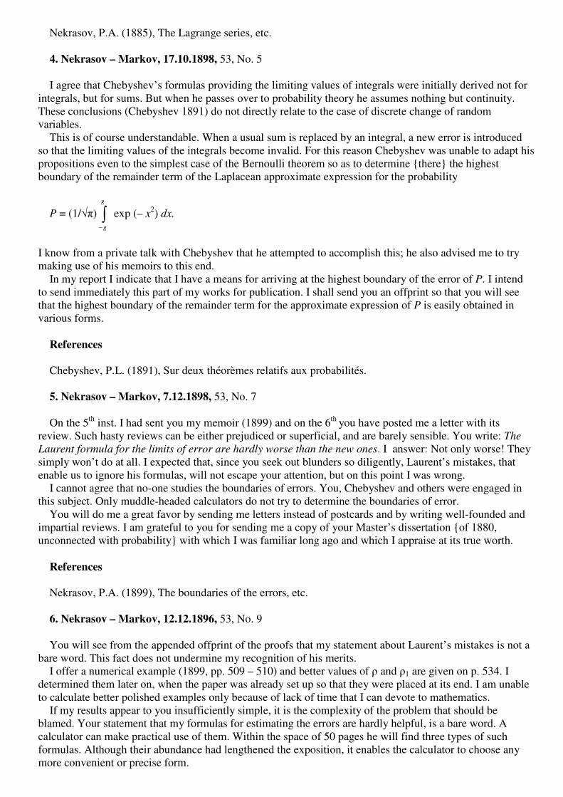
Nekrasov, P.A. (1885), The Lagrange series, etc. 4. Nekrasov – Markov, 17.10.1898, 53, No. 5

I agree that Chebyshev’s formulas providing the limiting values of integrals were initially derived not for integrals, but for sums. But when he passes over to probability theory he assumes nothing but continuity. These conclusions (Chebyshev 1891) do not directly relate to the case of discrete change of random variables. This is of course understandable. When a usual sum is replaced by an integral, a new error is introduced so that the limiting values of the integrals become invalid. For this reason Chebyshev was unable to adapt his propositions even to the simplest case of the Bernoulli theorem so as to determine {there} the highest boundary of the remainder term of the Laplacean approximate expression for the probability

P = (1/��) �−

g

g

exp (– x2) dx.

I know from a private talk with Chebyshev that he attempted to accomplish this; he also advised me to try making use of his memoirs to this end. In my report I indicate that I have a means for arriving at the highest boundary of the error of P. I intend to send immediately this part of my works for publication. I shall send you an offprint so that you will see that the highest boundary of the remainder term for the approximate expression of P is easily obtained in various forms. References Chebyshev, P.L. (1891), Sur deux théorèmes relatifs aux probabilités. 5. Nekrasov – Markov, 7.12.1898, 53, No. 7 On the 5th inst. I had sent you my memoir (1899) and on the 6th you have posted me a letter with its review. Such hasty reviews can be either prejudiced or superficial, and are barely sensible. You write: The

Laurent formula for the limits of error are hardly worse than the new ones. I answer: Not only worse! They simply won’t do at all. I expected that, since you seek out blunders so diligently, Laurent’s mistakes, that enable us to ignore his formulas, will not escape your attention, but on this point I was wrong. I cannot agree that no-one studies the boundaries of errors. You, Chebyshev and others were engaged in this subject. Only muddle-headed calculators do not try to determine the boundaries of error. You will do me a great favor by sending me letters instead of postcards and by writing well-founded and impartial reviews. I am grateful to you for sending me a copy of your Master’s dissertation {of 1880, unconnected with probability} with which I was familiar long ago and which I appraise at its true worth. References Nekrasov, P.A. (1899), The boundaries of the errors, etc. 6. Nekrasov – Markov, 12.12.1896, 53, No. 9 You will see from the appended offprint of the proofs that my statement about Laurent’s mistakes is not a bare word. This fact does not undermine my recognition of his merits. I offer a numerical example (1899, pp. 509 – 510) and better values of � and �1 are given on p. 534. I determined them later on, when the paper was already set up so that they were placed at its end. I am unable to calculate better polished examples only because of lack of time that I can devote to mathematics. If my results appear to you insufficiently simple, it is the complexity of the problem that should be blamed. Your statement that my formulas for estimating the errors are hardly helpful, is a bare word. A calculator can make practical use of them. Within the space of 50 pages he will find three types of such formulas. Although their abundance had lengthened the exposition, it enables the calculator to choose any more convenient or precise form.

I see no justice in your public opposition to my report devoted to Chebyshev. It is unfair to interrupt a man who only opened his mouth to speak, and to accuse him when he still wants to continue his speech. I shall of course have to repulse your attack in press even though the periodicals will regrettably be loaded with special incidents again and again. But what can we do if academicians like such relations and customs! References Nekrasov, P.A. (1899), The boundaries of the errors, etc. 7. Nekrasov – Markov, 18.12.1898, 53, No. 12 After acquainting myself with the poor quality of the articles (1898; 1899) {Markov} sent to me, I find that their author had quite deserved a public protest against his actions. References

Markov, A.A. (1898), Sur les racines de l’équation, etc. --- (1899), The law of large numbers and the method of least squares. 8. Nekrasov – N.F. Dubrovin {Permanent Secretary, Imp. Acad. Sci.; written after receiving an offprint of

Markov (1898) from its author}, 18.12.1898, 52, No. 1 I venture to inform you that […]. Academician A.A. Markov had no moral right to publish this paper (or another one, – Markov (1899)). If it is not too late, it is desirable to withdraw the first one from the Academy’s periodicals; otherwise, to allow me to publish my protest in the Izvestia {of the Academy}. In corroborating the validity of these desires, I have the honor to report […] In August of this year Professor […] B.Ya. Bukreev […] read out my summary at the Congress […]. It was published at the same time (Nekrasov 1898) and its offprints were sent out to many Russian mathematicians including Markov […] My summary contains a briefest statement explaining in what domain I had accomplished my works. These are intended for publication, which I am compelled to postpone for the time being because of putting my calculations in order. […] {The summary} contains only a naked indication of my findings (partly absolutely new, partly old ones, but demanding explanation and development). I posses their demonstrations, but have not provided them and promised to do so at publication. In making such a statement to the Congress, I confided in the protection of the scientific community, hoping to ensure the possibility of at least completing my work calmly and free from those encroachments upon it which occur in the absence of scientific bodies when sometimes homo homini lupus est. Everywhere in the scientific world such a statement is usually sufficient for preventing anyone from pushing the toiling scientist away from his path and wilfully occupying his place. It is self-evident that my summary, aiming at such goals, could not include because of its brevity either a listing of the contributions of my predecessors, or an explanation of their relation to my work. However, among all of them, I felt it necessary to single out the name of Academician Chebyshev, to devote my summary to him. Such a summary should hardly have been subjected to any criticism with respect to its contents since my work was still to be expounded. Nevertheless, Markov came out against it in his correspondence with me accusing me of injustice to the late Chebyshev, distrusting my conclusions and doubting the correctness of my proofs, still unpublished. For my part, I have confirmed, in this correspondence, that I mean to publish my proofs after which he will be able to judge them. It occurred, however, that Markov did not want to wait and acted absolutely otherwise. In his papers mentioned above, which were prompted by my summary and the relevant correspondence, he published his proofs of what was both accomplished by me in a somewhat different form and stated to the Congress in my summary. Namely, Markov offered a proof of the well-known theorem by which Chebyshev had substantiated the method of least squares and which was not yet proved with all rigor and in such generality. True, I have thus lost only some part of my findings rather than all of them. However, if my just interests will not be defended, then I fear that Markov will take advantage of his standing as well as of my credulity that guided me, when I openly stated the plan and the results of my investigations to the Congress, and deprive me of all the rest by pushing me away from my contemplated path here also. I protest against

Markov’s actions and I am asking the Academy of Sciences to defend me, to prevent Markov from using its periodicals against me as a tool for attaining undesirable goals. However, my protest is not confined to this end. After being informed by a letter from Markov that he intends to come out with the abovementioned papers, I have again asked him not to interrupt the course of my works and to give me the opportunity of expressing myself completely. In reply, I have received an indecent postcard showing that Markov had understood my request in a very peculiar manner. Don’t worry, he wrote, how can I mention works that do not deserve any attention? I pass them over in silence. It is obvious therefore that I am pushed away from my path in a most inadmissible way. I am prepared to pay but little attention to the rudeness of this phrase since it humiliates to a greater extent those who utter it than those to whom it is addressed. I cannot, however, fail to protest against Markov’s actually silencing my works which I stated in my summary. The result of this will be that the scientific community, reading the periodicals of the Academy, will attribute to Markov priority in that, to what he is not entitled. Such a deliberate failure to mention my works even more violates both my rights and academic decency. […] The mathematical section of the Congress […], attended by many most competent experts, appraised my summary differently and expressed its thanks to me in writing (the ������� (Diary) of the Congress, p. 329). Addendum, n.d., 52, No. 6

Markov informs me that he had not borrowed anything from my works, and that his first letter to Prof. Vasiliev […] 1 was written before he received an offprint of my summary. I regard it as a debt of justice to explain that I have never thought to declare that he had borrowed something from my proofs (not yet even published). Nevertheless, in my opinion Markov should not have published his own proofs either, since he knew that I had obtained the same results before he did, and declared to the Congress my intention of publishing them. Markov’s first letter to Vasiliev is dated 23 September whereas my summary dated 3 August was read out on 26 August. Lastly, Markov had received its offprint not later than on 1 October, – that is, before his papers were published. Given these circumstances, he could not have failed to understand the situation and was able to postpone the publication of his papers. […] Independently from this, Markov in all probability came to know about the existence of my summary even before he received its offprint since it was mentioned not only in the Diary of the Congress, but also in various newspapers not excepting the Novoe Vremia. In addition, those participating in the Congress from all the university cities (including Petersburg) could have informed Markov in more detail about the contents of my summary. […] I am greatly interested […] in the aspect of principle […]. As far as I know, editors of serious foreign scientific periodicals do not allow {their} authors such a deliberate wilfulness. […] Notes 1. {Markov’s paper (1899) is composed of extracts from several of his letters to Aleksandr Vasilievich Vasiliev (1853 – 1929), then at Kazan University; his works pertained to the theory of functions of a real variable and history of mathematics. All the letters were dated.} References Markov, A.A. (1898), Sur les racines de l’équation, etc. --- (1899), The law of large numbers and the method of least squares. Nekrasov, P.A. (1898), The general properties of mass independent phenomena, etc. Translated in this book. 9. Markov – Konstantin Konstantinovich Romanov {President, Imperial Academy of Sciences}, Dec.

1898, 52, No. 7 Your Imperial Highness, N.F. Dubrovin, the Permanent Secretary of the Academy of Sciences, has sent me copies of three letters written by Nekrasov and informed me that Your Highness will be pleased to receive from me a written

explanation with regard to their subject-matter. I flatter myself with hope that Your Highness will find the desired explanation in the lines below. 1) Nekrasov’s letters are a combination of unbelievable demands with contradictory and groundless arguments. 2) Nekrasov would desire to forbid me to criticize his summary, and, at the same time, he is dissatisfied at my not having mentioned it. I, however, am thoroughly convinced that Nekrasov’s summary cannot be cited without remarking that some of its propositions are well-known and badly formulated by him and that the other ones are doubtful; and it is also doubtful that the author has their rigorous demonstrations at hand. Neither is it possible to refer to Nekrasov’s summary without indicating that, being devoted to the memory of Chebyshev, it mentions one of his memoirs leaving without attention the other one, closer to it in subject-matter. 3) To refute my opinion that his summary does not deserve attention, Nekrasov offers the following reasoning: {his letter to Dubrovin, see p. 89 above}: The mathematical section […] appraised my summary

differently and expressed its thanks […]. This argument cannot be regarded as convincing even if admitting, as Nekrasov states, that many most competent experts have attended the Congress. Indeed, he himself {p. 88}says: Such a summary should hardly have been subjected to any criticism […]. A summary that cannot be criticized, cannot be adequately appraised either; and, without an appraisal, the gratitude mentioned by Nekrasov is only an act of politeness and proves absolutely nothing. 4) Nekrasov’s statement that my opinion described above was expressed so as to justify some wilfulness does not agree with the truth. This wilfulness only exists in his imagination and I do not therefore have to defend it. 5) I could have replied in kind to the passage from my indecent, as Nekrasov says, letter quoted by him. However, such usage of private correspondence seems indecent to me. I shall only indicate that he probably forgot the contents of his letter when he resolved to declare that the passage was an answer to his request not

to interrupt the course of his works. I ought to say that his request is absolutely inappropriate especially now, when Nekrasov became acquainted with my papers (1898; 1899) 1. 6) The superficiality of Nekrasov’s claims is proved by his own words {p. 89}: In his papers[…] which

were prompted by my summary and {our} correspondence, he published {my discovery. He} offered a proof

of the {Chebyshev theorem}that was not yet proved with all rigor and in such generality. Elsewhere {p. 90} we read: I regard it as a debt of justice to explain that {Markov had not} borrowed something from my

proofs (not yet even published). It follows that he deals with a well-known theorem and that its proof expounded by me was not borrowed from Nekrasov. For the sake of a better understanding, I consider it useful to note that I borrowed the formulation of the theorem from that Chebyshev’s memoir (1891) which Nekrasov had not mentioned. To the conditions stipulated by Chebyshev I have only added one more without which the theorem can lose its validity as shown in my paper (1899). I could not have borrowed this condition from Nekrasov’s summary which does not mention it. I conclude that, since this condition is lacking there, he does not possess a rigorous proof of the theorem; its non-rigorous demonstrations are known for a long time now. 7) Modifying his claims in his additional letter, Nekrasov {letter to Dubrovin, p. 90} says:[…] Markov

should not have published his own proofs either, since he knew that I had {already} obtained {them} […]. These words do not agree with the truth since my papers (1898; 1899) do not contain any finding about which it would have been possible to say that it was derived by Nekrasov, and that he declared his intention of publishing it to the Congress. 8) Nekrasov’s statement that my papers are prompted by his summary and letters is refuted by the fact that, both in subject-matter and methods, these papers adjoin my previous works and are far from his contributions published to this day. Furthermore, already in 1895 I have clearly indicated the essence of my paper (1898). Note

1.{This sentence is crossed out in the original manuscript.} References

Chebyshev, P.L. (1891), Sur deux théorèmes relatifs aux probabilités. Markov, A.A. (1895), On the limiting values of integrals.

--- (1898), Sur les racines de l’équation, etc. --- (1899), The law of large numbers and the method of least squares. 10. Nekrasov – Markov, 20.12.1898, 53, No. 13 I consider it my duty to notify you that I have lodged complaints with the Permanent Secretary of the Academy of Sciences and the Kazan Physical and Mathematical Society 1 against your wilful attitude towards my works which is inadmissible according to the generally accepted behavior among scientists and which consists in publishing that, which forms a part of my completed but not yet published works. I was unable to devise any other means for protecting myself against your encroachments upon my works. And, above all, I could not count on your voluntary amendment of the harm that you caused me. I shall be glad, however, if you will voluntarily satisfy me by supplementing your publications (1898; 1899) with adequate explanations. You will get to know about the substance of my claims in more detail from the Permanent Secretary. […] 2 Notes 1. {Markov’s paper (1899) was indeed published in the periodical of that Society. Nothing is known about Nekrasov’s complaint with the Kazan Society.} 2. {Nekrasov added a few lines discussing the debates that followed Kovalevskaia’s study of the rotation of a solid about a fixed point. Markov was prominently involved in these, see Tsykalo (1988, pp. 73 – 74).} References Markov, A.A. (1898), Sur les racines de l’équation, etc. --- (1899), The law of large numbers and the method of least squares. Tsykalo, A.L. (1988), A.M. Liapunov. M. (R) 11. Dubrovin – Markov, 26.3.1899, 54, No. 1 Our Imperial President instructed me to ask you to soften somewhat the expressions in your statement about Nekrasov’s article. His Highness considers your expressions unfit for the minutes of the Academy and would have preferred to replace them by those words which he wrote on the appended proofs. I venture to hope that you will find it possible to consent to this request. I would have come personally to discuss this subject with you, but I do not feel myself well enough and am therefore compelled to trouble you with this message. I shall wait for your answer and for the return of the proofs now being sent. 12. Nekrasov – Markov, 24.12.1898, 53, No. 15 I do not grudge your borrowing something from my works; but I feel bitter because you partly pushed me away from my path which I had previously announced at the Congress (on 26 August) thus accomplishing some of what was already done by me but not yet published. My summary was read out at the Congress by Bukreev and announced in the Diary {of the Congress} and in various newspapers (not excepting the Novoe

Vremia) before you wrote your letter to Prof. Vasiliev 1. Although I have not mentioned a number of memoirs of my predecessors, the Chebyshev paper not excluded, this cannot be compared {?} since, as I have explained it more than once, the publication of my works, where all of them will be mentioned, is forthcoming. In addition, nothing can be taken from Chebyshev, whereas all my work could be taken away from me since it was trustfully reported to the Congress but not yet published. Anyone, who does not respect the customs of scientific bodies, can take all my findings away from me profiting by my credulity as well as by the special conditions that do not allow me to publish my completed works too quickly. True, you took away from me not the most important part at all since my works extend much further by indicating not only the limits of magnitudes, but also the deviations from the limit. But who may guarantee that you will not win over from me these parts as well since I have no time to publish them right now? I cannot fail to say that you (1899) 2 have expressed many vague and even strange statements. Notes

1. See Note 1 to Letter 8.} 2. {Nekrasov mentioned two pages that followed the long passage from the Gauss letter to Bessel.} References

Markov, A.A. (1899), The law of large numbers and the method of least squares. 13. Nekrasov – Markov, 2.1.1899, 53, No. 17 How can I make you to understand that all your instructions about my report, about its missing portions and your relevant doubts constitute a premature and unmannerly intrusion upon another’s work now under publication. I explain once more: My report is only the beginning of a discourse on my accomplished works meant for publication. It is only a heading, and, as such, it plainly cannot be of a desired comprehensiveness. Instead of patiently waiting for me to complete the publication of my works before judging their missing parts and shortcomings, you are intruding upon them with your unbidden instructions to which it is difficult to answer anything, and even demanding gratitude for all this. These uninvited good deeds are bad in that you benefit me by my own money that I already had in my pocket. Furthermore, in your articles you have published what I had previously accomplished in another form and thus impudently pushed me away from my path which I had previously claimed. […] 1 Thus, intrusions (sometimes successful, sometimes not at all) on the domains of others is your speciality rather than mine. Even your Master’ s dissertation 2 was, according to my conviction, an intrusion (although successful) in the domain of Chebyshev and Posse 3. Notes 1. {I have again (see Note 2 to Letter 10) omitted a few lines concerning Kovalevskaia.} 2. {See end of Letter 5.} 3. {Konstantin Aleksandrovich Posse (1847 – 1928) worked in mathematical analysis and the theory of functions.} 14. Nekrasov – Markov, 18.4.1910, 53, No. 11 I agree that it is time to discontinue our private correspondence because of its uselessness and the exhaustion of all that was possible and necessary to say by each of us. I shall, however, consider it a matter of honor and justice to strive for publishing the “Necessary explanations” caused by the note (1910) where Academician Markov discredits my works in which everything essential is true and preserves its worth 1. I personally feel no animosity towards my opponent. On the contrary, I wish him all the best. Note

1. {Nekrasov’s “Necessary explanations” were hardly ever published.} References Markov, A.A. (1910), Correcting an inaccuracy. 15. Nekrasov – Markov, 20.4.1910, 54, No. 2 I can only sympathize with Markov’s desire to publish the entire correspondence which clears up much since I prefer publicity of discussion to decisions made in private. […] In all justice, my note, “A necessary explanation”, relating to the foundations of the law of large numbers, should be published in the same journal as was (Markov 1910). And perhaps Vasiliev, who is able to understand our correspondence, will publish it […] I am asking you to show this letter also to Vasiliev so as to find out who of us should visit Bekhterev 1. Note

1. {Vasiliev was mentioned in the Note to Letter 8. V.M. Bekhterev (1857 – 1927) was a psychiatrist and neuropathologist.} References Markov, A.A. (1910), Correcting an inaccuracy. 16. Nekrasov – Markov, 20.12.1913, 55, No. 5 {The beginning of this letter is translated in part 2} […] The term pure mathematician, although recognized in our vocabulary, yields to definition with difficulty and is not interpreted by our mind in an unique way. If it means pure observer, would not then mathematics become too subjective, and, like metaphysics, not compulsory to anyone? Should not exactly the theory of probability be not too pure a mathematics so as to throw a bridge from subjectivism to external reality, a bridge travelling through experience? Statistics is cumulative experience 1. I intend to go to Moscow, and can continue the correspondence with A.A.M. after returning back. Note 1. {On Nekrasov’s philosophical views about probability see also Letter 3 in Part 2 and his own letter to the mathematician K.A. Andreev of 7 March 1916 (Chirikov & Sheynin 1994, pp. 160 – 161). In the second case Nekrasov stated that the theory of probability was the foundation for a sweeping mathematical induction in the

area of moot but vital problems (Poincaré, Pearson, N.A. Umov). Umov (1846 – 1915) was an eminent physicist, but his contribution to the theory, if any, remains unknown.} References Chirikov, M.V., Sheynin, O. (1994), Correspondence of Nekrasov and Andreev.

17. Sergei Oldenburg (Academician, Permanent Secretary, Imp. Academy of Sciences) – Markov, 5.11.1915, 57, No. 1

Physical and Mathematical Department, Extract from Proceedings 14 Oct. 1915, §494 5 Nov. 1915, No. 2095 494. The Member of the Council of the Minister for Public Education 1, Privy Councillor P.A. Nekrasov […], in his letter of 29 Sept., had informed the Vice-President that: During many years I am engaged in a scientific debate on the theory of probability and differential and integral calculuses with Academician A.A. Markov 2, with whom Prof. K.A. Posse partly sides. I side with the schools that were headed by Academician V.E. Imshenetsky and Prof. N.V. Bugaev who defined the principles of mathematics in a different way. The stages of our polemic can be discerned in the appended papers Nekrasov (1915a) and in Nekrasov (1915b). In addition, the records of the Physical and Mathematical Department of the Academy of Sciences contain my protests of 1898 and 1910 against Markov’s wrong attitude towards my report (1898) which includes a critical review of the relation of Chebyshev’s great theorem on mean values to his second theorem (Chebyshev 1891). Markov then published his modified form of the Chebyshev’s second theorem (1898b; 1899) concealing from his readers that his modification was a corollary of my report. For my part, I do not at all, and shall not keep away from continuing our scientific dispute provided that it will be carried out by generally accepted academic means. The matter, however, is that, independently from the debate in the press and scientific bodies, Markov, beginning with 1898, worries me out with a great number of rude postcards 3. He had failed to comply with my long-standing request to quit sending me such postcards, but, until it remained possible to consider the nature of his sharp words if only barely endurable, I had to

answer him, attempting, on the one hand, to keep as precisely as possible to his expressions, and, on the other hand, not to raise the degree of their sharpness. The latest postcard, in which, in spite of its extreme sharpness, I still grudgingly considered it possible to answer, and my answers were as follows. Postmark 25 Sept. of this year. If P.A.N. does not desire to keep for himself the title of slanderer, he will take into account the following information. In A.A.M’s lectures (1898a) it is said, on p. 42: It is important to remark that we do not reckon zero, the limit of an infinitesimal, among the set of its values”. The same is said on p. 50 of the edition of 1901 – 1902 4. No signature. My first reply postcard of 26 Sept.: If A.A.M. will not take back his published slander contained in his pamphlet (1912) and in (1915), then he has no right to cite his lithographed lectures which P.A.N. is not compelled to know. Is it not a scandal that A.A.M. says one thing in his lectures and something else in his polemic attacks. A.A.M. got muddled up in semitruths and won’t hear of the connections between the parts of the tree of science. There exist two prototypal kinds of infinitesimals rather than one kind since there are two types of changes, unbroken and discrete (N.V. Bugaev). My second postcard of the same date: I shall mention A.A.M’s information about the definition of infinitesimal as given in his lectures of 1898 and 1901 – 1902 in my next paper, but along with indicating another definition (the true one), offered by N.V. B – v and me 5. The substance of Markov’s reply postcard postmarked 26 Sept. was such: I am not interested in the absurd definitions put forward by N.V. B – v and P.A.N. I hope that the slanderer P.A.N. will not be allowed to publish any other paper: he had already sufficiently revealed himself. All that, which is contained in Markov (1912) as well as in Markov (1915), is true. P.A.N. is not compelled to hear about my lectures, although he should have learned the principles. However, only an unsensible or a foul person can attribute to me statements that I never uttered. A.M. Having objections to the essence of this postcard, I do not answer it since the form of the expressions contained there is already of a definitely criminal nature which might be considered, independently from the problem about the infinitesimals, in the chamber of a Justice of the Peace. I believe, however, that an appeal to a Justice of the Peace, so as to stay the intolerable form of debate adopted by a member of the Academy, is not proper for a member of the Council of the Minister of Public Education because of the high standing of their institutions. Therefore, I have the honor of asking most humbly Your Excellency to discuss two questions by the Collegium {?} of the Academy: 1) Is the usage of rude and abusive expressions, which Markov permitted himself to make in his postcard of 26 Sept., compatible with his status of member of the Academy of Sciences? 2) Can the Collegium {?} of the Academy of Sciences ensure me that in future Academician A.A. Markov will restrain himself from writing me insulting letters? Only such kind of a guarantee can make it possible for me to abstain from the abovementioned less desirable means of exerting influence upon him. I beg to inform me about the subsequent events. I have sent a copy of this letter to His Excellency, the Minister of Public Education. It is resolved to answer P.A. Nekrasov that the Academy cannot engage in problems having to do with the private correspondence and polemics of its members. It is also resolved, according to a proposal put forward by Academician A.A. Markov, to constitute a Commission for discussing some problems touching on the teaching of mathematics in school. The following academicians are elected to the Commission: A.A. Markov, A.M. Liapunov, V.A. Steklov; and Corresponding Members D.K. Bobylev, N.Ya. Tsinger, and A.N. Krylov. The Permanent Secretary is charged with assembling the Commission which will then elect its chairman. Permanent Secretary, Academician Sergei Oldenburg Notes 1. {The appropriate modern term would apparently be … Council of the Ministry …} 2. {A few years before that Markov and Nekrasov agreed to discontinue their correspondence (see Letter 14). Obviously, however, letters were still being exchanged between them.} 3. {Nekrasov (1916) soon published six of the latest ones (1915 – 1916).}

4. {Markov became member of the Commission mentioned at the end of this letter. It published its report (translated in this book) where (p. 72) Markov’s qualification remark about the values of infinitesimals was explained by considerations of convenience.} 5. {B – v stands for Nikolai Vasilievich Bugaev (1837 – 1903) who worked in mathematical analysis and number theory, was a partisan of discrete mathematics and a philosopher and Nekrasov’s teacher. Nekrasov hardly ever hesitated to use such loose expressions as true definition. Cf. Note 2 on p. 28 and Notes 3 and 4 on p. 51.} References

Chebyshev, P.L. (1891), Sur deux théorèmes relatifs aux probabilités. Markov, A.A. (1898a), �������������� � ���������� (Differential Calculus). --- (1898b), Sur les racines de l’équation, etc. --- (1899), The law of large numbers and the method of least squares. --- (1912), A rebuke to Nekrasov. Translated in this book --- (1915), On the draft of teaching the theory of probability, etc. Nekrasov, P.A. (1898), The general properties of mass independent phenomena. --- (1915a), Theory of probability and mathematics in high school. --- (1915b), Reply to K.A. Posse’s objections. --- (1916), ������� �� ��, ��������, � .�. (The High School, Mathematics and Scientific Training of Teachers). Psb.

Part 2

The Method of Least Squares; Reactionary Views;

Teaching of Probability in Shool

The Laplacean Theory of the Method of Least Squares Simplified by a Theorem of Chebyshev

P.A. Nekrasov

Foreword by Translator

Nekrasov is seen here as a very strange author. He attributes an interpolational application of the method of least squares to Legendre; he wrongly describes the difference between Laplace and Gauss concerning least squares; without offering anything new he claims to consider his subject more attentively than others did; and he throws in a few financial terms apparently believing that he thus fosters the application of the theory of probability to economics. Below, I also include translations of four of Nekrasov’s relevant letters to Markov. ********************************************************** [1] The method of least squares that is used for determining a group of v unknowns x, y, z, …, w on the basis of a very considerable number m of observations (m > v) has a three-fold application in accord with the opinions of Legendre, Laplace and Gauss (Tsinger 1862). Legendre’s point of view is interpolational; it has no regard to the theory of probability but it concerns other branches of mathematics. For example, it is applied for determining the parameters !, µ, … of an interpolational function F(x; !; µ; …) of the variable x by means of a given group (of a table) of the values of an empirical function (Laurent 1908). It has to do with the mathematical formulation of the empirical laws of nature expressing a smooth course of variation that admits the application of analytic functions to the abovementioned formulation. Laplace and Gauss, however, issuing from differing points of view, applied the method of least squares to problems closely connected with the theory of probability. The difference of these points concerns both the moment of the discussion {of the observations} and the chronological sequence of the facts. Laplace justifies the method for future observations, – he reasons as a quantity surveyor, – whereas Gauss substantiates the same method on the basis of made observations, – he is able to revise the facts, to collate suppositions with reality and to apply the doctrine of posterior probabilities.

The Laplacean theory of the method of least squares was developed by Cauchy, then by Bienaymé, Tsinger (1862), Laurent (1908), Chebyshev, Sleshinsky (1892), Markov (1899) and others. Because of the involved derivation that Laurent bases on the use of the Dirichlet discontinuity factor, this theory is known to be restricted by assumptions sometimes kept back. It is possible to simplify this derivation of the method and to separate clearer the doubtful from the certain by means of the Chebyshev theorem from his memoir (1867). This theorem is distinguished by its distinctness and simplicity of its demonstration. [2] Here is a simplified derivation of the method of least squares. Let the system of initial equations be akx + bky + … + pkw – lk = �k , k = 1, 2, …, m (1) where lk is the result of observing the linear function akx + bky + … + pkw

of the unknowns x, y, …, w and �k is the error of the respective future {?} observation. The probability �k (�k) d �k that the error �k will take a definite value depends on the nature of the observations. The type of the function �k (�k) remains undefined; however, let the observations and the measured forms of functions be such that the observations are independent one from another and the expectations of the errors �1,�2, …, �m are zero, i.e., S �k (�k) �k d �k = 0, k = 1, 2, …, m (2) where the integrals S extend over all the possible values of the variable �k which constitute a discrete or continuous series. Let the expectations of the squares of the errors remain always finite and not exceeding a given boundary. Denote them by Mk: Mk = S �k (�k) �k

2 d�k, k = 1, 2, …, m. (3)

We note in passing that the numerical values of the errors �1, �2, … and therefore of the magnitudes M1, M2, … depend not only on the functions �k (�k) but also on the choice of the units of those concrete phenomena whose values are denoted by symbols x, y, … 1 A large unit decreases the absolute values of both �k and Mk; an s-fold decrease of the unit increases Mk by the factor of s2. Multiply each of the equations of the system (1) by an indefinite multiplier !k and add up these equations {these products}. We obtain the equation

x� ak!k + y� bk!k + … + w� pk!k –� lk!k = � �k!k (4)�

Introduce then new conditions

� ak!k = m, � bk!k = … = � pk!k = 0. (5)

They connect only v of the indefinite quantities !1, !2, …, !m; the rest (m – v) of them remain yet arbitrary. Owing to the conditions (5), the equation (4) becomes

x = (1/m)� lk!k + (1/m)� �k!k = (1/m)� lk!k + ( /m), (6)

= �1!1 + �2!2 + … + �m!m. (7) Applying the theorem of the Chebyshev memoir (1867), we denote a given positive and very small number by t; and we suppose that the probability of the inequalities – t < /m < t (8) is P. According to that theorem, P should satisfy the inequalities

1 > P > 1 – (H/mt

2) (9) where H = (1/m)[ M1!1

2 + M2!22 + … + Mm!m

2]. (10) Since t is assumed to be very small, the quantity /m, that, according to our supposition, satisfies the inequalities (8), might be neglected so that the equality (6) will become

x = (1/m)� lk!k. (11)

For this solution to correspond to the highest value of the probability P it is necessary for its lower boundary indicated in the inequalities (9) by K = 1 – H/mt

2 (12) to take its maximal value 2. Here, we consider K as a function of the variables !1, !2, …, !m connected by conditions (5). This conditional maximum of the quantity K also corresponds to the conditional minimum of the function H as defined by the equality (10). When determining the conditional minimum of the function H in accord with the well-known plan {!}, we shall at first calculate the absolute minimum of the function

H – X (� ak!k − m) − Y� bk!k − … − W� pk!k

where X, Y, …, W are new, yet indefinite quantities, v in number, independent from the variables !1, !2, …, !m. Later on we shall take into account the conditions (5). Thus we find, in addition to system (5), a system of equations determining the sought minimum of function H; indeed, we obtain the system of equations 2 Mk!k = Xak + Ybk + … + Wpk, k = 1, 2, …, m. (13) Systems (5) and (13) are in general sufficient for determining (m + v) quantities !1, !2, …, !m and X, Y, …, W. It is easy to eliminate the !’s after which we get the following system of v equations

X� (gkakak/m) + Y� (gkakbk/m) + … + W� (gkakpk/m) = 1,

X� (gkbkak/m) + Y� (gkbkbk/m) + … + W� (gkbkpk/m) = 0, …(14)

for calculating the supplementary quantities X, Y, …, W. Here, the quantities gk = 1/(2Mk), k = 1, 2, …, m, are proportional to the weights of the future observations. Note that each coefficient of the unknowns X, Y, …, W in each equation of system (14) represents the arithmetic mean of the terms gk qk rk. If these terms are always finite, then, for any very large value of number m, the system (14) generally (exceptional cases do exist) provide finite values for all the v unknowns X, Y, …, W. Consequently, system (13) will also furnish finite values for the !’s so that the quantity H determined by equality (10) will be finite with K being very close to 1. It follows that the assumptions (8), reducing the error ( /m) of the approximate equality (11) to a negligible quantity, will be almost certain. This certainty, this high rate of confidence, is the main advantage of the derivation justifying the Laplacean theory of the method of least squares. This justification is elementary, but with respect to rigor or generality it is not inferior to less elementary substantiations. [3] Exceptions to this general reasoning that disturb the standard (the rule) of the plausibility of the justification (of the conclusion) occur when the determinant D of the system of linear equations (14) either vanishes or is so close to zero that the !’s determined by systems (14) and (13) become infinite or very large or indefinite. In these exceptional and not infrequent cases, to which one or another paradoxical state of the conditions and realization of the experiments or observations corresponds, the quantity K (see (12)) can evidently

deviate far from 1 thus lowering our rate of confidence in the conclusions. In other words, in such paradoxical situations there exist sufficient grounds for perceiving in advance the unreliability of the proposed derivation of the unknowns x, y, …, w by the method of least squares, and, consequently, for searching out other methods of {their} plausible determination and perhaps for modifying the conditions and realization of the observations so as to exclude doubtful situations. We have examined the method of deriving only one unknown, x. Repeating our reasoning, we can extend the same method onto the other unknowns, y, z, …, w by transferring them, one after the other, on the first place. The expressions of the unknowns x, y, …, w should still be identified with the Gauss formulas obtained by the method of least squares; that is, we ought to show that these expressions coincide with the formulas for those values of x, y, …, w for which the function g1�1

2 + g2�2

2 + … + gm�m

2,

that includes the quantities �k derived from equations (1), becomes minimal. We convince ourselves in this fact by comparing, in the generally known way, the indicated values of the variables with the derived expressions for the unknowns. It follows that the Gauss method, issuing from another point of view, leads to the same expressions for the unknowns x, y, …, w. This formal (with respect to the algebraic expressions of the results) coincidence of the Gauss and the Laplace methods corresponds in the best possible way to the practical collation of the expected as formulated in the Laplacean sense of quantity surveying with the reality in the Gauss sense of revision 3.

Addendum I have connected the well-known Laurent’s proof (1873) which he repeated elsewhere (1908) with a theorem from Chebyshev’s memoir (1867) that simplifies this substantiation. I failed to recall Yarochenko’s memoir (1893a; 1893b) that includes the same simplification, and I consider it my duty to correct my oversight 4. Independently from this simplification, which is due to Yarochenko, my article contains summary indications of both normal and paradoxical cases occurring in the theory of the method of least squares. In this sense my paper goes further than Yarochenko’s memoir 5. These indications depend on the substantiality of H and of the determinant D of system (14). I link these quantities with my own explication of the general indications of such a connection of events when the Chebyshev theorem sometimes characterizes the deviation of a complicated mass phenomenon which it described from the narrow conditions of the law of

large numbers; in other words, when it characterizes the instability or the catastrophism of that phenomenon. In my book (1912, pp. 304 – 307; 318 – 319; 324 – 326; 338 – 339; 343) I explain in more detail, and for dependent and independent variables, the notion of paradoxical and catastrophic cases as worked out by means of the Chebyshev theorem. Notes

1. {A hardly necessary remark.} 2. I ask the readers to compare this point of my reasoning with the appropriate point of the derivations provided by other authors who apply either the Dirichlet discontinuity factor or other equally complicated formulas. 3. {Nekrasov repeats his strange statement first formulated in the beginning of his memoir. Also see his letter to Markov of 20 Dec. 1913 below. Laplace assumed a large number of observations and issued from his non-rigorously proved central limit theorem whereas Gauss introduced an integral measure of precision (the variance) as his criterion for treating a finite number of observations.} a4. {The first to connect the method of least squares with the Chebyshev theorem was Usov (1867).} 5. {Indications concerning special cases were generally known at the time.} References Chebyshev, P.L. (1867), Des valeurs moyennes. Laurent, H. (1873), Traité du calcul des probabilités. Paris. --- (1908), Statistique mathématique. Paris.

Markov, A.A. (1899), Law of large numbers and method of least squares. Nekrasov, P.A. (1912), �� ��� ��� �� ��� (Theory of Probability). Sleshinsky, I.V. (1892), On the theory of the method of least squares. Zapiski matematich. Otdelenie

Novoross. Obshchestvo Estestvoispytatelei, vol. 14, pp. 201 – 264. (R) Tsinger, V.Ya. (1862), �� � � ���������� ������ � (Method of Least Squares). M. Master Diss. Usov, N.A. (1867), A remark concerning the Chebyshev theorem. MS, vol. 2, pp. 93 – 95 of second paging. (R) Yarochenko, S.P. (1893a), On the theory of the method of least squares. Zapiski Novoross. Univ., vol. 58, pp. 193 – 208 of second paging. (R) --- (1893b), Sur la méthode des moindres carrés. Bull. sci. math., sér. 2, t. 17, pp. 113 – 125.

Unpublished Letters from Nekrasov to Markov on the Method of Least Squares

Archive, Russian Academy of Sciences, Fond 173, Inventory 1 {The additional numbers, e.g., 55, No. 4, show the place of the letters in Fond 173}

1. 18 Dec. 1913, 55, No. 4

I think that we should not speak categorically either about an absolute validity or a complete unfitness of the derivations justifying the theory of the method of least squares because the theory of probability as a foundation of these derivations generally leaves room for an indefinite precise analysis. I, for my part, attach indefiniteness to the derivations contained in my paper and A.A.M. will easily see this in the lines which I underscored on the appended offprint of my paper (p. 6). In the applications of the Chebyshev theorem it is in general necessary to distinguish and examine à priori the normal cases conforming to the laws {of nature} and paradoxical instances not complying with the laws {?}. I differ from Yarochenko and Tichomandritsky 1 and many others in having this spirit of doubt and investigation, of critical attention. Taking into account the exceptions indicated in my paper, I do not see why A.A.M. thinks that the reasoning there provided will not do at all. It will do for something!.. The theory of probability mainly creates supplementary and indirect judgements and patterns, valuable and necessary together, or in connection with other data and with the conclusions made by the exact natural sciences. 2. 20 Dec. 1913, 55, No. 5 In the normal case the maximal value of K will be close to 1 because, if the given t is too small, the standard requirement of the method of least squares includes the assumption that m is sufficiently large for ensuring the smallness of H/mt

2. Your objections are correct but they concern either a paradoxical realization of the experiments (the determinant D is close to zero) or the case of an insufficiently large number m. I distinguish the points of view of Gauss and Laplace by the moments with regard to the experiment: the first one is posterior, and the second one is prior. It is more opportune to judge à posteriori because more data are available, but this point of view is delaying, it lags behind, drags after the event 2. 3. 14 Jan. 1914, 55, No. 7 In a letter written in December, A.A.M. examines the lines of my paper {examines the sentence that includes formula (12)}. He perceives there a mistake made by Yarochenko and me. Studying it, A.A.M himself established some kind of a connection between P and K, and, issuing from the indicated lines, cooked up a syllogism of Russian thinkers: if 1 > P1 > 0.9, 1 > P2 > 0.8, (A) then

P1 > P2. (B)

Not only a Western, but even a Russian thinker will certainly not resign himself with such a syllogism. However, it does not follow from the examined lines that a functional connection exists between P and K, the less so a monotone connection. On the contrary, no definite functional dependence is assumed. Consequently, inequalities (A) cannot lead to a compulsory inequality (B); P1 < P2 and P1 = P2 are also possible. The word highest in the accused lines above are too laconic, it should have been replaced by a dictum {!} which evidently follows from the context of the entire paper and expresses the idea that the unknown and indefinite quantity P is closer to 1 and tends to 1 as m increases to �. 4. 16 Jan. 1914, 55, No. 9 Don’t cast lies on Prof. Yarochenko & Co. A.A.M. attributes such syllogisms to Yarochenko that cannot be drawn from his works as their necessary corollaries. A.A.M. mistakenly considers the writings of those mathematicians who do not agree with him as a crime against mathematics. The dogma of justice, courts and policemen is needed for distinguishing between crime and virtue, but mathematics does not require this. Let A.A.M. explain who indeed are the judges and policemen in mathematics and where are its legal dogmas. I think that mathematics is guided by logic and criticisms formulated by pure intellect that does not need to bring criminals to court or to encourage virtues. Mathematics only requires proofs and fundamental definitions (axioms) which precede demonstrations. And axioms are admitted or otherwise voluntarily, without any compulsion or legal auto-da-fé 3. Notes 1. {Nekrasov apparently referred to Tikhomandritsky, M.A. (1898), .�� � ��� ��� �� ��� (Course in Probability Theory). Kharkov.} 2. {See the end of this letter in Part 1 of this book.} 3. {Markov wrote stupid across the last lines of this letter.}

The Theory of Probability and the Struggle against Sedition

V.I. Bortkevich (Ladislaus von Bortkiewicz)

Foreword by Translator

This paper is interesting fort two reasons. First, it describes Nekrasov as a (petty) philosopher and a reactionary thus complementing our acquaintance with this prominent mathematician. Second, the author was an outstanding statistician whose thoughts about Nekrasov (and thus his general political viewpoint) remains unknown outside Russia. Moreover, even in his former homeland his paper was hardly read since it appeared abroad in a rare periodical, and, even so, apparently only in some of its copies. I myself have seen two copies of the journal in question which did not contain Bortkevich’s article, and one copy, in the rare books department of the Russian National (former, Lenin State) Library, including it. The article was signed by a single letter “B” but later on Bortkevich (1910, p. 353) claimed his authorship. My present copy is a photostat duplicate of a copy previously possessed by B.I. Karpenko, a student of Chuprov, and kindly made for me by Dr. A.L. Dmitriev (Petersburg). Bearing in mind my general aim, I decided that a large part of the paper below is not really interesting; however, because of Bortkevich’s importance, and the obvious difficulty in getting hold of this source, I am reprinting the portions, omitted in the translation, in the original Russian. The spelling V. I. (Vladislav Iosifovich) Bortkevich conforms to the Russian version of his name; from 1901 he lived and worked in Berlin as Professor at the present-day Humboldt University. ********************************************************** [1] In governmental and security circles it is long since being usual to distinguish sciences according to the degree of their loyalty. In olden days the natural sciences were considered as the most dangerous, but in our time the same property is attributed to social and state sciences. The former professor of mathematics at Moscow University and at present the curator of the Moscow educational region, P.A. Nekrasov invented a peculiar method of rendering them harmless in the political sense and of directing them to the true path of serving orthodoxy, autocracy and national unity 1. In his booklet, he (1902) appears as a convinced partisan of

applying the theory of probability to studying social phenomena. This idea is not new, and, generally, the author’s arguments in its favor are not original since they are of a theoretical nature. His deliberations on the various kinds and degrees of dependences between phenomena in Chapt. 1 deserve relatively most attention. It is striking, however, that the author did not at all see fit to have a look at the special literature on the philosophy and logic of probability theory, or, what is even more surprising, at later works on its application to statistics. At least by reading Czuber (1898; 1902 – 1903) Nekrasov could have become convinced in that, beginning with the time of Quetelet, this domain had not remained in stagnation and that others have already achieved the revision of the foundations of Queletet’s social physics

2, and, for that matter, much more successfully as is proved by certain positive results about which Nekrasov evidently has no information. And, excepting some items, even the earlier special literature about Quetelet remained unknown to Nekrasov. Had he been acquainted with the pertinent writings, �# #$ � $% �&'() *+, ,�# #�-.+/(%� 0'%.�-& 1/#�'� &-(2($�3'� $( 4.�1&�1�/�% / �.&�(5 6%�)% 7)%'%$�#/, #�,(1�� 4.#��/#.%,(8�5 �#,-% 2.%$�3 4#2���/�2'( �(- -(- �(/$+' �(/$# -.���-#9 *+)# #*.(8%$# /$�'($�% $( 1&8%1�/%$$+% $%4#1)%�#/(�%):$#1�� � 4.#��/#.%,�3 -(- /# /2;�3�(5 6%�)%, �(- � / 14#1#*(5 �5 /+.(<%$�3. =( 7�#, '%<�& 4.#,�', &-(2+/(%�13 � / �� ��� ������� >$1#$(, -#�#.#;# ;. =%-.(1#/ 1#/1%' $(4.(1$# &4.%-(%� / 4%.%�%)-% &,%$�3 6%�)% «$( 4#2���/$+9 )(�» (c. 9). ?%<�& �%' 1(' Nekrasov is guilty of quoting Quetelet in a biased manner. He passes over in silence such well-known pronouncements as ce qui se rattache à l’espèce humaine considérée en masse est de l’ordre des faits

physiques – �2.%,%$�3, #*.(.&<�/(@8%;# /1@ �8%�$#1�: &1�)�9 ;. =%-.(1#/( �#-(2(�:, ,�# «6%�)% � A@11'�):5 /4#)$% #�$#.#�$+ 4# B�)#1#B1-�' /2;�3�('» (�(' <%). C/)%,%$�% (/�#.( A@11'�):5#' � D���$;%$#', -#�#.+% 4.�'%$3)� - �11)%�#/($�@ #*8%1�/%$$+5 3/)%$�9 4# 1�(��1��,%1-#'& '%�#�& �%#)#;�,%1-&@ �#,-& 2.%$�3, $(/.3� )� /+�%-(%� �2 �#;#, ,�#*+ #$ 4.�2$(/() �5 ������ ����� *#)%% 1#/%.E%$$+'� 1.(/$��%):$# 1# 15%'#9 4#2���/�1�#/, - -#�#.#9 #$ #�$#1��13 1�.#;# -.���,%1-�. F%�: � A@11'�):5&, � D���$;%$& 1#/%.E%$$# ,&<�+ �% $(&,$#-B�)#1#B1-�% -#$G%4G��, 1/32($$+% 1 �%#.�%9 /%.#3�$#1�%9, -#�#.+'� �(- �#.#<�� ;. =%-.(1#/. H-#.%% /1%;# /+1#-(3 #G%$-( $(2/($$+5 (/�#.#/ 1# 1�#.#$+ ;. =%-.(1#/( #*I31$3%�13 %;# 3/$+' 4.�1�.(1��%' -# /1%'& *#<%1�/%$$#'&. J(-, /# '$#;�5 '%1�(5 *.#E@.+ (c. 105, 127, 133) ��%� .%,: # <�2$%#4�1($�35 1/. 4#�/�<$�-#/ � 4#�/�<$�G, .%-#'%$�&%'+5 $( 4%./#' '%1�% / ,�1)% $(&,$+5 '(�%.�()#/, �#)<%$1�/&@8�5 )%,: / #1$#/($�% #*8%1�/%$$#9 $(&-� *&�&8%;#. K1#*%$$+% $(�%<�+ /#2)(;(%� (/�#. (c. 79) $( ����/ ��� �� �������� ��� ������ � ������� �� ,

�������/ 0����� ����� ����� �� ���� �� ��,

������/1�� ������� � �������� �� ������� �� �� -��������� �

���� � �� ���� ��� � ,��, � 2 � �� � , ��� �������� �������,

� �����/1�� �1� �� ��������� � � ���� � ������������ �

���� ����� � ��� �����. 2 �1� ��� � ������� -������ ,

��� � ������� [��������� ������� � ;. =%-.(1#/ (c. 78) $(2+/(%� ��������, �� �������� �� � � ����/������ � ����� �

���������� ��] � ����,�� [?], � ��� � ���, � �����

�� ��������, /���������� � �1�������� � � ���� � ,�������

������ ��������-�� *��� � ������� � ���� � �������

��� � ���� � � � �� ����, � ��� ������ ����� �������

���� � *����. ������ ����� ��������*�, ��������, ������

��,��� �� �� ���� ���� , ������� , ��������, �� ������ ,

���������� ����� �� ����. 0����������� �� ������ ��������

������� - ������ , ����������� (�����, 3 , ��, 3 ���� �,

� � ������, ,��� 4.&.� �� � � ��,��) � ������� ���� �

�� ������� ��*���� ������� -�������� �� ��� ��� ������ � ���

� �� *�������� ������. &��� ��� *���� ������� ������ �

�� ������ ��� � ��������, �������, ���� , ,������ ���� � �

� � �� �, , � � � � �,��� � �� ���������� � ����� . [2] =(1-#):-# 4.%�%$2�� ;. =%-.(1#/( $( 1#)��(.$#1�: 1 )&,E�'� 4.%�1�(/��%)3'� .&11-#9 '+1)� / $(&-%, B�)#1#B�� � )��%.(�&.% #1$#/(�%):$+, /+31$��13 �2 �():$%9E%;# �2)#<%$�3 %;# /2;)3�#/. J%4%.: <% $% '%E(%� &1�($#/��:, ,�# 4# ,(1�$#'& /#4.#1& #* #�$#E%$�� 4#2���/�2'( �, 4.%<�% /1%;#,

1('#;# 6#$�( - 4.#*)%'% # �/�<&8�5 1�)(5 �1�#.�,%1-#;# 4.#G%11( /#22.%$�3 ;. =%-.(1#/( $% $(5#�3� 1%*% 4#��/%.<�%$�3, '%<�& 4.#,�', 1# 1�#.#$+ �%5 4.%�1�(/��%)%9 .&11-#9 �1�#.�,%1-#9 $(&-�, -#�#.+5 #$, /%.#3�$#, <%)() *+ 1,��(�: 1/#�'� %��$#'+E)%$$�-('�. > �'%@ / /��& /%1:'( #*1�#3�%):$&@ 1�(�:@ 0.H. L(44#-M($�)%/1-#;# / �� ������ ��������� #* #1$#/$+5 4.�$G�4(5 1#G�#)#;�,%1-#9 �#-�.�$+ 6#$�(, ;�% 1#�%.<��13 &-(2($�% $( �#, ,�# 6#$� $% �#):-# / 1/#%9 � ����� #�/%) /%1:'( /��$&@ .#): /#)%/#'& $(,()&, «$# / 1&8$#1�� &<% / 1/#%' 6&.1% 4.��() /#)% 2$(,%$�% ,&�: )� $% 1('#1�#3�%):$#;# B(-�#.( / 3/)%$�35 #*8%1�/%$$#9 <�2$�» (c. 428). N.(/�(, ,�# ;)(/$#% #*/�$%$�% ;. =%-.(1#/( 4.#��/ 6#$�( � 4#2���/�2'( B#.'&)�.&%�13 �' �(-�' #*.(2#', ,�# #$� �1-)@,�)� «�2 �1�#.�,%1-#9, 7-#$#'�,%1-#9 � @.���,%1-#9 $(&-�» $% 4.#1�# «/#)@», ( «1/#*#�$&@ /#)@» (c. 73). =# 7�& 1/#*#�$&@ /#)@ ;. =%-.(1#/ #4.%�%)3%� �)� /%.$%% #4�1+/(%� �(-�' #*.(2#' (c. 76): �� � ���� � �� ������ ����/������ � ��� ��� ���� ������

��� � ���/1�� ������� �������, �� ������1�� (� ��� � � �����

�������) �� ��� ��� ��� ������, � � ���� �� � ������ ���

� � � ���� � ���,��� �. F �.&;#' '%1�% (c. 128) ;#/#.��13, ,�# «1/#*#�$(3 /#)3 �#)<$( �.(-�#/(�:13 -(- #1#*(3 41�5�,%1-(3 1�)(, 1)(;(@8(313 �2 /1%5 �&E%/$+5 1�) (1%.�%,$+5 � &'1�/%$$+5) -(- �5 .(/$#�%91�/&@8(3.» J(-�' #*.(2#', ;. =%-.(1#/ ,�# � �#-(2+/(%�13 �(-<% %;# 11+)-('� $( L%9*$�G( � L(4)(1(, / -#�#.+5 #$ $(5#��� 4#��/%.<�%$�% 1/#%9 �#,-% 2.%$�3, #�$@�: $% 3/)3%�13 1�#.#$$�-#' �� � �� � �� / 1#*1�/%$$#' 1'+1)% 1)#/(, ( )�E: 4.#��/$�-#' �%5 &,%$�9, -#�#.+% 1/#�3� $( $%� .#): )�,$#9 41�5�-� �, / ,(1�$#1��, /#)%/#;# '#'%$�( / �1�#.�� � 1#G�#)#;��. =# / �(-#' 1)&,(% /#2/#��'#% �' $( 6#$�( � 4#2���/�1�#/ #*/�$%$�% 3/)3%�13, -(- 7�# /��$# �2 4.�/%�%$$+5 1)#/ ;. L(44#-M($�)%/1-#;#, /# /13-#' 1)&,(% 1)�E-#' #;&):$+'. 0 ,�# -(1(%�13 �# 3-#*+ 1&8%1�/&@8%;# ;)&*#-#;# .(2)�,�3 '%<�& 6#$�#' � 4#2���/�1�('� /##*8%, 1 #�$#9 1�#.#$+, � 6%�)%, 1 �.&;#9, / �5 /2;)3�(5 $( 2$(,%$�% /#)%/#;# $(,()(, � �# &4.%-#/ 4# (�.%1& >$1#$( � �.. / 4%.%�%)-% 6%�)% $( 4#2���/$+9 )(�, �# / 7�#' #�$#E%$�� ;. =%-.(1#/ &<% 4.3'# $%4.(/. =�,%;# $% 1�#�)# *+ �1-&1$+' 4#�*#.#' G��(� 4.#�2/%1�� �& #4%.(G�@, -#�#.#9 / .(2*�.(%'#9 *.#E@.% 4#�/%.;13 6%�)%, 1 6#$�#', ,�#*+ 4.�*)�2��: %;# - 4.%�1�(/��%)3' 5#�3 *+ �#;# <%, 1�#): G%$$#;# / ;)(2(5 ;. =%-.(1#/(, �%#)#;�,%1-#;# /2;)3�( $( 4.#G%11+ #*8%1�/%$$#9 <�2$�. F1�.%,(@8�'13 & 6%�)% /+.(<%$�3' ��� 2��� ,1�, � ��� �� ��� (1. 74), 2( -#�#.+% G%4)3%�13 ;. =%-.(1#/, � 2( 4.#4&1- -#�#.+5 / 1##�/%�1�/&@8%9 G��(�% #$ �(- 1�.#;# #1&<�(%� >$1#$(, '#<$# *+)# *+ 4.#��/#4#1�(/��: 2���� � �1��� �2 Cours de philosophie positive 6#$�(. N%.%� 1&�#' ;. =%-.(1#/( 4#2���/�1�+ � 4#1)%�#/(�%)� 6%�)%, $%4.(/�):$# %;# 4#$�'(/E�%, #-(2+/(@�13 /�$#/$+'� %8% � /##*8% / &'()%$�� .#)� '#.():$#-�$�%))%-�&():$+5 1�). =# /%�: O#-):, -#�#.+9 ;)(/$+' #*.(2#' �'%%�13 �&� / /��&, 1,��() 1('+' '#;&8%1�/%$$+' B(-�#.#' �1�#.�,%1-#;# .(2/���3 &14%5� 4#)#<��%):$#;# 2$($�3. D�# )� $% �$�%))%-�&():$(3 1�)(? 0 4# /#4.#1(' $.(/1�/%$$#1�� O#-)@, -(- �2/%1�$#, *+)( ,&<�( ��%3 7/#)@G�� $.(/1�/%$$+5 4#$3��9 – �.%. �( ��%3, -#�#.(3, /##*8% ;#/#.3, � /+2+/(%� #�4#. 1# 1�#.#$+ 4.�/%.<%$G%/ (*1#)@�$#9 '#.()�. [3] H -%�)%��2'#' / #1/%8%$�� O#-)3 � 0�#):B( F(;$%.( ;. =%-.(1#/ (1. 73) 4.�/#��� / 1/32: � �� � ,������� ( � � �������� � �� ��������) ���������� .����

+�����, 5�,�����, 4 ��� � ��., / -#�#.#' (1. 87) ����� ���������

���� � � ��� ������ � *���� ������ ������/ ����

���� � ,������� ���, � ������ �� � �� �� ��� ���� ����/��

��� � ������� ���� �,� ���/�� ��� �� ���/1�� ��������.

=% /�(/(31: / #G%$-& 7�#9 3/$# $%4.(/�):$#9 5(.(-�%.�1��-� 7-#$#'�,%1-#;# '(�%.�()�2'(, '+ $% '#<%' $% /+1-(2(�: &��/)%$�3 4# 4#/#�& �#;#, ,�# (/�#. �8%� -#.$� 7�#;# $(4.(/)%$�3 & 4#2���/�1�#/ � 6%�)%. 6#'& $% �2/%1�$#, ,�# B�)#1#B1-�% #1$#/($�3 2(�'1�/#/($+ ?(.-1#' � D$;%):1#' #�,(1�� �2 P%;%)3, #�,(1�� �2 '(�%.�()�2'( , #� -#�#.#;# $(1�#38�% 4#2���/�1�+ #�-.%8�/(@�13 3 ? K�$(-#, 4# ;. =%-.(1#/&, �)%�/#.$#% /)�3$�% -%�)%��2'( 4.#1��.(%�13 �():E%. «O#)%% �#/%.,�/+5» �2 �1�#.�-#/ � @.�1�#/ 4#1)%�$�9 4.�/%) «- &/)%,%$�@ &�#4�3'�» (1. 6) /1)%�1�/�% �2/.(8%$$#;# 4#$3��3 # 5(.(-�%.% 2(-#$#/, -#�'� &4.(/)3%�13 ,%)#/%,%1-(3 <�2$:.

�� ������� ���� �������� � ���� � *���� ����� � ������

��� � �������� ��� �� � *� � ��� �������/ �������� (�

*� ��������o) ��� ��� �� , � ������� ���*��� �

������������� � ������ � �������� ... )� � �����

, ��������� � � �1������ � *����, ����/1���� �� ����

����*�����, ����������� �� ����, �� ��� ��� ����� � ,

��,� ������� ����� ���, �� � ���� � ����*�� ��,���� ��

���, � �� , �1������ , �� ����� �, �� � � , � , ��� ���

� ����� ���� ����, � ��� �����/ �� �1������/ *����

�����,�/1�� � ������/1�� ���� �. 6 ��� ��� �������

� ��� , ����� ��� �1��� � ������ ��� ��� ���������

�� ��� ��*���� �� ��� ���/, � � ��� � ���������

���, ������ , �� , � �� �����/, � ��� � ���� ���-��� ������

�, ������ ��� �� ���� � ����� � ��� �, � ���� ���������

���/ � �� ��� ������ , �1�*��� ��� � ��� ����������. �� , ����� -�������� , �� ����� �� �����/ �� ,�� ����

-������ � ���� - � � �������� � � ������������� �����, �

� ��� ����� � � ������� � , � ����, � ������� ��� ���

����� � ��� ������ ���� � ���������� ���,, ������,��� � ��

��� ������, �, � ���� � ��� 1�� ���������,

���������� � � ������ � �� / (1. 89). N# 4#/#�& 7�#;# #�.+/-( $%):23, 4.%<�% /1%;#, $% 2('%���:, ,�# 1/32:, 3-#*+ 1&8%1�/&@8(3 '%<�& �%#.�3'� 6%�)% � 4#2���/�2'#' 1 #�$#9 1�#.#$+, � .(2$+'� $%#*�&'($$+'� .%B#.'('� � .%/#)@G�#$$+'� �/�<%$�3'� 1 �.&;#9 1�#.#$+, %1�: $% *#)%% -(- 4)#� �#1&<%9 B($�(2�� ;. =%-.(1#/(. M# 1�5 4#. 4.�$3�# *+)#, 5#�3 � *%2 �#1�(�#,$+5 #1$#/($�9, 1�(/��: 6%�)% / &4.%-, ,�# %;# �#,-( 2.%$�3 4.�/#���, $(#*#.#�, - 1#G�():$#'& -/�7��2'&. 0 �&� #-(2+/(%�13, ,�# �' /�#5$#/)3)�1: .%/#)@G�#$%.+.Q():, ,�# / .(2*�.(%'#' 1#,�$%$�� $% 1#�%.<��13 $( 1%9 1,%� *#)%% #4.%�%)��%):$+5 &-(2($�9. R�# -(1(%�13, 2(�%', / ,(1�$#1�� �# 1�(��1��,%1-#9 -(�%;#.�� � ��� , ����� *&��# *+ 1)&<(8%9 �)3 #4.(/�($�3 4#)���,%1-�5 4%.%/#.#�#/, �# 4.�5#���13 $%�#&'%/(�:, �'%%E: )� �&� �%)# 1 3/$#9 $%)%4#1�:@, 4.#�1�%-(@8%9 �2 $%/##*.(2�'#9 4&�($�G+ 4#$3��9, �)� <% 1 $%&�(,$+' -()('*&.#'. =(-#$%G, 4#1)%�$33 B.(2( / 4.�/%�%$$#' #�.+/-%, -#�#.#9 �'%)#1: / /��& $(�)%<(8�' #*.(2#' #5(.(-�%.�2#/(�: ��%()+ �%'#-.(��� � 1#G�()�2'(, '#<%� 1)&<��: #*.(2,�-#' ()34#/(�#1�� 4#)%'�,%1-�5 4.�%'#/ (/�#.(. [4] H�#�� #�'%���: �(-<% %;# #�$#E%$�% - -(4��()�1��,%1-#'& 1�.#@. S / �.&;#' '%1�% 1/#%;# 1#,�$%$�3 (1. 106) #$ &-(2+/(%� $( «1#/.%'%$$+% <%1�-�% #�$#E%$�3 �.&�( � -(4��()(» � 4.%�)(;(%� «&1�.($��: 7�& <%1�#-#1�: 4#1.%�1�/#' &1�.#91�/( -(11, 1�.(5#/($�3 .(*#,�5 � 4..» S, ,��(%' /1)%� 2( 7��', +� �����, � � ����������� ������ � ,���, ���� � �� ���������, ���� ���

��������� ���� ��� ���/1�� ��� ���� �/��� � ���*��� �,����� � � � ���� ���1� , �����

��� ���1���� ����.

=# (/�#. 4# /#4.#1& #* #�$#E%$�35 �.&�( � -(4��()( $% #;.($�,�/(- %�13 7��'� 2('%,($�3'�, '()# #.�;�$():$+'� 4# 1#�%.<($�@ � 5(.(-�%.$+'� �)3 $%;# )�E: 4# �#$& 4.%�38%9 %)%9$#1��. He also recommends the theory of probability to economists. According to his opinion, it can serve for softening these

cruel relations [between labor and capital] by fostering the introduction of the moral element into the very

estimation of labor and things, as it was attempted by Daniel Bernoulli and Buffon who offered a special

measure called moral expectation for estimating random sums (p. 106). All the irrelevance of this exhortation directed to economists is ascertained by an immediate acquaintance with the notion of moral expectation that first appeared in Bernoulli (1738) and served him for solving (wrongly, however) a problem from the theory of probability known as the Petersburg game

4. This notion has absolutely nothing in common with moral issues � #�$@�: $% '#<%� 1)&<��: 4.#��/#/%1#' «-.(9$% '(�%.�()�1��,%1-#9 #G%$-� ,%)#/%-(, 4.#�2/#�38%;# 5#2391�/%$$+% *)(;(», / -#�#.#9 ;. =%-.(1#/ &4.%-(%� 4#)���,%1-&@ 7-#$#'�@. Bernoulli had not even applied the term moral expectation but discussed lucrum (gain). So where is here the moral element and what is the aim of Nekrasov’s play upon words? But more is in store. Actually, economists,

for a long time now, and without awaiting indications from Nekrasov and certainly not for softening the relations between labor and capital, but in the sphere of the doctrine of value, made use of notions similar to those put forward by Daniel Bernoulli when solving the Petersburg game. I have in mind the theory of marginal utility whose connections with the constructions of Bernoulli were pointed out in the literature (von Wieser 1889, Intro.; Fick, in Bernoulli, translation, 1896, p. ix). Being a mathematician, Nekrasov is certainly not obliged to know this. But then, what compels him to admonish other specialists? [5] F4.#,%', 1#*1�/%$$# 7-#$#'�,%1-#9 #*)(1�� #$ -(1(%�13 )�E: /1-#):2:. H#G�():$+% � 4#)���,%1-�% �%#.�� � $(4.(/)%$�3 �$�%.%1&@� %;# ;)(/$+' #*.(2#' 1 *#)%% #*8%9 �#,-� 2.%$�3 . 6(- '+ /��%)�, 4#2���/�2', #�#<�%1�/)3%'+9 �' 1 '(�%.�()�2'#', � ������ ����� 6%�)% 4.�/#�3�, 4# %;# '$%$�@, - $%#*�&'($$+' .%B#.'(', - .%/#)@G��, �%'#-.(��� � 1#G�()�2'&. KE�*#,$+% 4.%�4#1+)-�, #�$#.#�$+% 1 #E�*-('� 6%�)%, (/�#. $(5#��� �(<% & L:/( J#)1�#;#, -#�#.+9 (1. 93) 7���,�� ��� ������ 8 , � � ����� ����� ��� �������� �� �

���*�����, ����������� � ��� � ���� �� �� � ����*�� (sic!) �

� ����/1���� ��� ������� ��������� � 9�����/ 8 *�/, –

���,�� ���� ��, , ������ , ���, �� � ��. On p. 94 he remarks: The wrong assumptions of Quetelet’s logical pattern led to the wavering of

the thought between the principle of slavery and anarchy since it is lacking

in a proper device for measuring reasonable freedom and reasonable

constraint. Let us see now how Nekrasov extracts this device from the theory of probability and the precise logic of

inductive sciences. In this respect, his point of departure is the notion of mutual independence of random events which is of essential importance for probability theory. {Bortkevich quotes Nekrasov’s definition of independence of random events.}The notion of mutual independence of phenomena is obviously also applicable to man’s actions insofar as they yield to stochastic considerations. The author calls independence in this sense freedom, and then, as though not realizing at all the extremely tentative nature of such designation, he identifies this new mathematical concept of freedom now with a metaphysical, or rather psychological concept of free will, then with the political and social concept of freedom. Nekrasov needs such obvious and unwitty juggling for screening, as we shall see now, his reactionary longings with the authority of the theory of probability. He attains this goal, first and foremost, by distinguishing between worthy or beneficial and harmful freedom. The theory of probability, as he states, reveals the true notion of freedom, and, according to his opinion, offers its precise viewpoint for distinguishing between the two kinds of freedom. Judging by some of his remarks, it would be desirable to understand his words in the sense that the theory of probability, or, more precisely, statistical observations, which are connected with some concepts of that mathematical discipline, enable to establish the nature and the measure of the influence of certain legislative enactments, of the state regime, of government policy on social life. Thus, objecting to the Tolstoy doctrine of non-resistance to evil, Nekrasov (p. 94) remarks that induction could have proved it wrong: The abolition of judicial repression of evil manifestations of free will,

would have led to the heightening of the probability of crime and to an

actual rise in crime. [6] Here, he considers it unnecessary to check experimentally that a given legal institution (the criminal law and the ensuing judicial repression) is a reasonable constraint and that its abolition would have led to unnecessary and harmful freedom. But in other cases the decision about the reasonableness of constraints and worthiness of freedom would have been made only through revealing, by comparative statistics, the consequences of those enactments and institutions which constrain or liberate. F#� - -(-#9 $%5��.#9 � #*+�%$$#9 '+1)� 1/#���13 4.%�%$G�#2$#% &�/%.<�%$�% (/�#.( (1. 26) *&��# �%#.�3 /%.#3�$#1�%9 (!) 4.�/#��� � �� ,�� ������ � ���� (!) ��� ��� � � �� � � ���

������ � ��� ������ � � �1���� ���, � �� � �������

[�������� �#<] � ���, � ��/ �� � �, ������ ���,

����� , ��� ������ , �1����.

Nekrasov, however, seems to recognize that such a statistical test, which enables to distinguish between worthy and harmful freedom, can sometimes be not altogether safe. Indeed, what should we do, if, in accord with the precise logic of induction, it occurs that some measure of constraint, established by the legitimate power, heightens the probabilities of such certainly negative phenomena as poverty, hunger, drinking, ignorance, enslavement by capital? You see, it is impossible to vouch for statistics5. Its conclusions can lead to the wavering of the foundations {of the Establishment}… And exactly these foundations should be saved and supported at all costs. We see that Nekrasov does not insist on applying the indicated statistical criterion, but, when appraising later on the various kinds of freedom, guides himself by a test of quite a different nature. This, it is true, has nothing in common either with probability theory or the precise logic of

induction, but, instead, offers the benefit of unusual simplicity and definiteness. The beneficial freedom, from the viewpoint of this new criterion, is that which conforms to the moral and civil laws, whereas the harmful freedom contradicts them (p. 113 et seq.). And, according to Nekrasov, the substance of a moral law is indicated by the Christian religion. H#�%.<($�% <% $.(/1�/%$$#;# 2(-#$(, 4# =%-.(1#/& (1. 100), &-(2+/(%�13 5.�1��($1-#9 .%)�;�%9: � ���� ������ � ������������ ����������� ��� � �� �� � ������������ ����,��, � ���� ������� ����������� ���

���,�� {$�-#;�(}, ��� ������ , �� ��/��. J(- ;)(1�� 4.�;#/#. (/�#.( $(� /1%9 �1�#.�%9 7��-�. R��(%' �():E%: ��������� � ���� � �� ��� ���� ��� �����������

��� � ���� ���� ����/ � ��� � ��� �� ��� �����

-����������� �/���, � ��� ����, � ��� �*� � �����

�� �� ��������� � � �� �� ��� �� �� ��������� �� � ,�������

������ � ����� � ��������� , ��� ��. 2 � ��� � �� �

�������� ���/1�� � 8 ,� �� ��� ���������, � ��*�

��, ������ ��� �����, ��� �� ���� � ���� � � �� ����

� ����� , �1������ , �,������, ���� ���� ����

� ���� ����� �/� � ���� ���������� � � ����, � ���,

������ �� �, �� � *� ��� ,�� � �*��� ������ ����� �

�/� ��/ � ���*���. N.�/%�%$$#% '%1�# '#<%� 1)&<��:, '%<�& 4.#,�', �)3 5(.(-�%.�1��-� .+G(.1-#;# #�$#E%$�3 ;. =%-.(1#/( - 4.#��/$�-('. K$ /##*8% �# � �%)# 4.�*%;(%� - 4#)%'�,%1-�' /+.(<%$�3' /.#�% ����������� � �� ��, �� ����� �� � � ������ (1. 103), � ��� � ��� (1. 121) � 4.#,. N.%�'&8%1�/# *#;#1)#/1-#9 '#.()� 4%.%� .(G�#$()�1��,%1-#9 (/�#. 4+�(%�13 �#-(2(�: � $( #1$#/($�� �1�#.�,%1-�5 �($$+5. C1�($#/�/ (1. 100), ,�# 4#$3��% # $.(/1�/%$$#' 2(-#$%, 4#,%.4$&�#% �2 *#;##�-.#/%$$#9 5.�1��($1-#9 .%)�;��, «%1�: /%.E�$( / )%1�/�G% $.(/1�/%$$+5 4#$3��9» � ,�# «7�& )%1�/�G& � $%#*5#��'# 4#)#<��: / #1$#/& �#,$#9 �$�&-��/$#9 $(&-� # 4.#3/)%$�35 ,%)#/%,%1-#9 �%3�%):$#1��», #$ (1. 102) /+1-(2+/(%�13 1)%�&@8�' #*.(2#' # .#)� 5.�1��($1�/( / �1�#.�� $(.#�#/:

2������ ���������� � ��������� � ������� � �*�� ����� �� �� � � ��������� ,

�� ������ , �� �����. 5� ������� ��� ���� ����������� ������. :����������

��� ��, �� ������, �� ,�� �������� � ��*� ���,�� ������ �� � �������, � �1��

� �� �� � � �������. 7���,����� �� ����������� ��� ��, � ����,����� , �����

�� ���������/ �� � � � � ���,��� � ��������, �������� � � ,��� �����, ��� ad absurdum ��*������ (!) 6 � �� �� ����*������ � � ����1����� �� *� �� � �� ����������� ��, ���

��� *������, ���� ���������/ ,�,�� ��/ � , � �������� ��� ���.

S 4#�#*$+% �1�#.�,%1-�% B($�(2�� /+�(@�13 2( 4#)#<%$�3 �� � ������� � ���� � ;. =%-.(1#/ #*)(�(%� 1'%)#1�:@ #*.(8(�:13 1 '%�#�#)#;�,%1-�'� &-(2($�3'� 4# (�.%1& 4.%�1�(/��%)%9 �1�#.�,%1-#9 $(&-� -(-, $(4.�'%., 4# (�.%1& 4.#B. F�$#;.(�#/( (1. 91 – 92)! K� .(11&<�%$�9 # $.(/1�/%$$#' 2(-#$% (/�#. (1. 104) 4%.%5#��� - 1##*.(<%$�3' # ;.(<�($1-#' 2(-#$%, / -#�#.#' � � *��� ��,������ ,������ ��� �� � � ����������� �������.

���������� � ,������ ����� �� ��� ����� 8 , � �

�� �� � ����/, � � ����� ,��*����� � �����/.

[7] 3��*������� ��� � ;. =%-.(1#/+' #�#<�%1�/)3%�13 1 1&8%1�/&@8�' .%<�'#', 1 �(- $(2+/(%'+' 4#)#<��%):$+' 4.(/#', � '+ $(4.(1$# 1�()� *+ �1-(�: / %;# �2)#<%$�� '()%9E�9 $('%- $( /#2'#<$#1�: .(2)(�( '%<�& 1�%1$%$�3'� ,��*����� , ��� �� � ��%()('� ���, � �� �

�� � ��. ��������, &1�($(/)�/(%'+% ;.(<�($1-�' 2(-#$#', #-(2+/(@�13 /1%;�( 1�%1$%$�3'� 1/#*#�+ $%*)(;#�/#.$#9. «T%.-#/:, ;#1&�(.1�/# 1 %;# &,.%<�%$�3'� � #*8%1�/%$$+% 4#�.(2�%)%$�3 � -)(11+» 1##*8(@� «#*8%1�/%$$#'& #.;($�2'& /$&�.%$$@@ 1�#9-#1�: , 1#�%91�/&@� 1-.%4)%$�@ %;# / #�$# G%)#%» (1. 107). =# (1. 137) ;�� ������ � �1��� � �*� ������� �� ��� � ������

� ����� , ���������, � � � ���� -������������� ���������

������, .�. � ��������� �����,�/1��� ��������� � ���������,

� ��� ���������/�� �����, ������� ������������

�� � �� � � �� ���� �1����. 5� ��� ����

-������������� ���� ��� ����/ ���� ������, ���/ �� /

*�� �/ ���������, ����/1/ ��� ������ �� ��. ��� � �

� ����� ���, � ���� �� ������� ���� ��� �1��������

�� ���� ������� ��� ��� � � � �� ��� � ������ �

�*����� � � ��� � ��� � ���� ������������ ,��*�������

���*�����, ���������� �������/1�� ������� �� �������

����� ���� �1���� ��� � ������� ������� ����� �, ����.

5� � �� � , ��� ���, � �� � ���� � � �� ����

� �� ��/ � ���� ��. K ������ � �� ��� -(- # �� ������ (!), $%�#4&1��'+5 � �.%*&@8�5 $%&-)#$$#;# 4.%1)%�#/($�3, ;#/#.��13 / .(2)�,$+5 '%1�(5 1#,�$%$�3, $(4.�'%. $( 1. 113, 109 � �.. The quoted passages show that the difference between the worthy and the harmful freedom as understood by Nekrasov coincides in the final analysis with the distinction between the allowed and the forbidden. [8] 6 �#'& <% .%2&):�(�& 4.�/#��� � �.&;#% //#��'#% (/�#.#' 4#�.(2�%)%$�% 4#$3��3 1/#*#�+: #$ .(2)�,(%� 1/#*#�& #�/)%,%$$&@ � -#$-.%�$&@. D�# 4#�.(2�%)%$�% 1/32($# 1 /2;)3�('� (/�#.( (1. 78) $( #�/)%,%$$+9 � .%():$+9 ��%()�2'. J#):-# 4#1)%�$�9, �.%. ��%()�2', «4.#/%.%$$+9 #4+�#' � $(*)@�%$�%' -#$-.%�$#9 �%91�/��%):$#1��», �'%%� 2(-#$$#% 4.(/# $( 1&8%1�/#/($�%.

<��� �������� ������� -������ , �������� ����� :����

-C������� � � ��� � �������, � ��������� �������� )��

������ � ) ������� � +���, � �� �� � � � ��� , � ��

� ���� ��� ���� �� � ��� ����� ��������� �������� �.

F 4.�'%$%$�� - /#4.#1& # 1/#*#�% �#,-( 2.%$�3 ������ , ��������� 4.�/#��� ;. =%-.(1#/( - .%2-#'& #1&<�%$�@ /13-�5 4#4+�#- 4#2(�'1�/#/($�3 1/#*#�$+5 4#)���,%1-�5 &,.%<�%$�9 & ,&<�5 $(.#�#/. «F13-�9 /%)�-�9 $(.#�», 4#&,(%� =%-.(1#/ (1. 124),

� �*�� �������� �� / ���� �����/ ������� -������/

���, � ��/ �� � �. 2 � ���, ��*� �� ���, ������ ����

�� ��*���� ��1�1��� �� � ��� ���� � ������� -������ �

���, � �� � �� � ��: ���� ������, ��� ���*���� � ��� �� ��.

F4.#,%', (/�#. $% /4#)$% /+�%.<�/(%� �#,-& 2.%$�3 #�$#1��%):$#1�� 4.� #G%$-% 4#)���,%1-�5 &,.%<�%$�9 .(2)�,$+5 $(.#�#/. J(-, '+ /��%)�, ,�# #$ (*1#)@�$# #1&<�(%� 1/#*#�& (11#G�(G�9 � -#()�G�9 (���� � �� � �, 4# %;# �%.'�$#)#;��), $% 1,��(31: 1 �%', ,�#, $(4.�'%., / 0$;)�� 7�#� �'%$$# /�� ��������� � ������� �� /1%'� 4.�2$(%�13 *%2&1)#/$# #*32(�%):$+' 7)%'%$�#' ���� ����� � ������� -������ � ���, � �� � �� � ��. A(�# / �.&;�5 #�$#E%$�35 #$, 4#-/���'#'&, $%4.#,: -#%-,%' 4#2(�'1�/#/(�:13 #� 0$;)��. K* 7�#' 1/��%�%):1�/&%� 1)%�&@8%% 5(.(-�%.$#% '%1�# (1. 132):

3 �������, � � ��� ���� ��� ������ �� � � �����������

�1�������� *����, ���� ��� � ���� ������� � ���� �����

��������� ��� ���� �� ������� �� � �� � � ��. ������,

��������, ��,����� , � �������, ��/1�� � �� �� � � �/�����

,��*���, �� ���� � �� �� �� ���� � ���� � ����� �� ���

��*� �������� � ��������� ��� ���,� ������� , . 2 ����

����� � �1������ � *���� 6�,��� � ���� �������� �

���� ���� ��������� �� �� ����� �� ������� �� � �� � � ��

� ������ �� � �� �� � � ��������� � �1������ � �

, ��������� � *����. ������� ����1��� �� � ��� ������

���������� � ��������� �� �� �����, � �� � �� � �� ���

����� ��������� , ���� *���� ��� � �. =�� ����� , , �

� �*�� � ������ � ��� �1�, ���,� ����������/ ��������/,

, � �,� � ���� ������� ���� ����� � ����/ �

� ����/1�� ���� �� � � ��. �������/1�� ��� �����/

�� � ��������� � � ,�/ ���� �� � � �� �� ��� ��� ���

��� � ��������/ � ����������� ������� ������ ���� �������.

This appeal for unflinching repression and corporal punishment is as though the finale of the philosophical-political treatise of this obscurantist scientist. In itself, his adopted viewpoint of an obtuse, unscrupulous and irreconcilable conservative is not original or interesting, but the methods which he applies here for justifying it deserve attention. A thoughtless application of the theory of probability for solving social and political issues; the choice, as his main object of debate, of a scientific direction (Queteletism) that, in a sense, is obsolete and in any case has no part in the current Russian thought; an absolute inability to orient himself with regard to various doctrines and systems; the flirt with the now popular philosophical idealism 7; a meek and unconditional worship of the temporal and the ecclesiastic power; and a rather confused exposition accomplished in a curious pseudo-scientific and self-invented jargon, – these are the main features characterizing Nekrasov’s criticism of free-thinking and advocacy of moral and physical violence. Is not all this an indication of scarcity and weakness of the intellectual and moral power in the camp of the modern guardians of law and order? [9] Nekrasov is a great admirer of Laplace not only in the mathematical, but also in the philosophical sense. For six weeks Laplace had to be Minister of the Internal Affairs, and Napoleon, to whom Laplace was obliged for being assigned to that post, became disappointed in him declaring that “he had looked everywhere for subtleties and introduced the spirit of the calculus of infinitesimals into management”. Like Laplace, Nekrasov is a mathematician, and he is also picked up for administrative activities. However, as we have seen, when the matter concerns social and political issues, he avoids subtleties even in the theory and does not care about excessive precision. He has a common appraisal and a common recipe for the enemies of the people and the order, for positivists, materialists, socialists, and worshipers of political freedom: all of these are sly political parties (p. 131), or cheats, windbags and parasites (p. 121); and only unflinching repression is appropriate with regard to them. Yes, unlike Laplace, Nekrasov hacks straight from the shoulder and it might be expected that his administrative career will prove more durable than that of the great French mathematician. In any case, his present contribution, even though not adding anything to his scientific reputation, will not apparently shake his administrative standing. It would have been a queer twist of fate, if, because of a misunderstanding, those

on the top will not be satisfied by Nekrasov’s experience in justifying the principles of firm power and

autocracy, as being necessary for the existence of our state, by means of the theory of probability whose main concepts do not at all include the notion of necessity. Notes

1. {The three words in italics constituted the essence of the officiasl motto in Czarist Russia.} 2. {This is the subtitle of Nekrasov’s reviewed book.} 3. U&):%, / Esquisse psychologique des peuples Européens, 2% �2�., 1903, 1. 468, / 4#)$&@ 4.#��/#4#)#<$#1�: ;. =%-.(1#/&, 2('%,(%�: Le positivisme d’Auguste Comte a sa partie idéologique: c’est la loi des

trois états, qui subordonne le mouvement social entier au développement

intellectuel, aux idées d’abord théologiques, puis métaphysiques, enfin

scientifiques et positives. Le comtisme français est aujourd’hui

l’antithèse du marxisme allemand.

4. {Actually, Daniel Bernoulli changed the conditions of this game as originally invented by Niklaus Bernoulli. The term moral expectation did, however, appear in Daniel’s memoir (cf. below), but only in a passage from Gabriel Cramer’s letter which Daniel quoted.} 5. His statement on p. 46 is apparently directed against the zemstvo statisticians: The best statisticians-observers in various branches are those educated

people who are in constant administrative contact one with another when

directing the course of business at hand. Management and statistics are

in essence inseparable.

{Bortkevich should have approved of the last phrase.} 6. Ad absurdum 2$(,�� � ����� ��. ?#<$# &*%���:13 / �1��$$#1�� -(-#9-$�*&�: '+1)� 4.�/%�%$�%' 4.#��/#4#)#<$#9 %9 '+1)�, 4&�%' &'#2(-)@,%$�9, - $%)%4#1�� (reductio ad absurdum). =# ,�# 2$(,�� «&*%���:13 / ,%'-$�*&�: - $%)%4#1��», 7�#;#, $#�# 4#)(;(�:, � 1(' ;. =%-.(1#/, / -(,%1�/% 14%G�()�1�( 4# �� � � ,���, $% / 1�)(5 #*I31$��:. O%2;.('#�$+% #*#.#�+ $% �#):-# 1 &,(1��%', $# � *%2 &,(1��3 )(��$1-#;# 32+-( /##*8% /1�.%,(@�13 & ;. 4#4%,��%)3 '#1-#/1-#;# &,%*$#;# #-.&;( �#/#):$# ,(1�#. F#� #*.(2,�- %;# 1��)3 (1. 134):

2������ �� � �� � � �� �� ��������� � ���*�1�� �� � ��������

����� ��������� � �����*���/, ���� � � ���������� � � , ,

�� ��� � ��������, � � � ����������/, � �� *�

���������� ��� � ������� ��� �� ��� ��� ����� � ,���� 1. S$�%.%1$# �(-<%, ,�# 4.�1�.(1��% ;. =%-.(1#/( - �.%/$%.&11-�' B#.'(' 32+-( ($(4.�'%., �������) &<�/(%�13 .3�#' 1 2)#&4#�.%*)%$�%' 1)#/('� �$#1�.($$#;# 4.#�15#<�%$�3. J(-, $( 1. 120 ;#/#.��13 #* ��%35 «*%2 �#1�(�#,$#;# B#$�( / #-.&<(@8�5 &1)#/�35». 7. S ,%;# '#<%� #<��(�: ;. =%-.(1#/ #� 7�#;# .&11-#;# $%#��%()�2'( -.#'% 1('#;# .%E��%):$#;# � $%�/&1'+1)%$$#;# #�4#.(? F 1�(�:% «6 5(.(-�%.�1��-% $(E%;# B�)#1#B1-#;# .(2/���3» ;. N.P. 2('%,(%�, ,�# «B�)#1#B1-�9 ��%()�2' � ;#1&�(.1�/%$$+9 4#2���/�2' $%4.�'�.�'+ 4# �&5&» � 4.�4�1+/(%� 2(1)&;& /+31$%$�3 7�#9 '+1)� F)(��'�.& H#)#/:%/& (�� ����� ���������, 1. 86). D�#, '%<�& 4.#,�', #��$ �2 �%5 '+1)��%)%9, 1 -#�#.+'� ;. =%-.(1#/ �'%%� $%#1�#.#<$#1�: 1,��(�: 1%*3 1#)��(.$+' � ,:% �'3 #$ #1#*%$$# ,(1�# 4.#�2$#1�� /1&%. References

Bernoulli, D. (1738), Specimen theoriae novae, etc. German translation with Einleitung by L. Fick: Leipzig, 1896. Bortkevich. V.I. (1910), Aims and concepts of scientific statistics. Zhurnal Ministerstva Narodn.

Prosveshchenia, vol. 25, No. 2, pp. 346 – 372 of second paging. (R) Czuber, E. (1898), Die Entwicklung der Wahrscheinlichkeitstheorie, etc. Leipzig.

--- (1902 – 1903), Wahrscheinlichkeitsrechnung und ihre Anwendung, etc. Leipzig. Nekrasov, P.A. (1902), >�� � ��� � � ,���, � �.�. (Philosophy and Logic of the Foundation of Quetelet’s Social Physics). Von Wieser, F. (1889), Der natürliche Wert. Wien.

Report of the Commission to Discuss Some Issues concerning the Teaching of Mathematics in High

School

A. Markov, A. Liapunov, V. Steklov, N. Tsinger, D. Bobylev, A. Krylov

The Commission, consisting of six members, […], had three sittings, […], and, after a thorough discussion of the issues, unanimously arrived at the conclusions expounded below together with the appropriate detailed considerations. 1. The Zhurnal … published a draft (Nekrasov 1915a) compiled by the Member of the Council of the Minister of People’s Education 1 P.A. Nekrasov and P.S. Florov, Director of the Uriupinsk non-classical school {Realschule}, on the introduction of the theory of probability into the curriculum of the high school; a summary of the relevant opinions of some persons officially requested to comment by the Department {?} of the Ministry[…]; and a digest of this material complete with notes and conclusions by Nekrasov. For specialists in mathematics, the groundlessness of this draft is obvious, but there exists a serious apprehension that the official standing of one of its authors can facilitate the carrying out of the draft into the school life. Concerning this draft, the Ministry officially questioned some persons selected by the Department of People’s Education {?}, but they had not applied to the most authoritative institutions, – to the Academy of Sciences or to the national universities. The possibility of realizing the draft was not denied at all and one of its authors (Nekrasov 1915a, No. 2, p. 124) even indicated that, if aiming at its speedy implementation, an execution of a two-hour {weekly} course was possible as a narrow bureaucratic arrangement demanding no legislative sanctions. Some of those questioned also thought that the realization of the draft was desirable or admissible as an experiment, but none of them adequately appraised it in essence. This circumstance compelled Markov (1915) to offer a short but definite assessment of the project. This, as well as a related paper by Posse (1915), caused the appearance of two new articles by Nekrasov (1915b; 1915c) where he attempted to put into practice his interpretation of the main notions and definitions of {mathematical} analysis which are already included in the school curriculum, – namely, of the concepts of limit and infinitesimal. Mathematicians are acquainted with Nekrasov’s views for a long time now, but, until having been only discussed in special mathematical periodicals, they could have been considered harmless. The situation changes when they are disseminated by an official organ that the school teachers cannot help considering an authoritative guide to scientific-pedagogic issues. Therefore, the Academy of Sciences, as the most important scientific estate of the Russian Empire (Charter, §1), that might enter into everything concerning education (§8) and is obliged to care about the dissemination of education in general and to direct it to the general weal (§2b), – the Academy ought to express its judgement about the main mistakes and the wrong (hence, harmful) ideas spread by Nekrasov so as to put them into common school use. Before discussing the introduction of the theory of probability into the school curriculum which is still only planned, the Commission will dwell on Nekrasov’s interpretation of the elements of analysis that are already taught in the high school. 2. Without going yet into detail, the Commission believes it necessary above all to indicate the following. Nekrasov attempts to establish the existence of two different directions in the mathematical science, of two different scientific schools disagreeing with each other in their understanding of the elements of the science and struggling one with another. He (1915b, p. 15) sets off one school having a nasty theory of knowledge with another one whose alleged leaders were Academician V.G. Imshenetsky and Prof. N.V. Bugaev (Nekrasov, letter to the Vice – President of the Acad. Sci. {translated in this book}) to which he also attributes himself. In other instances he (1915b) attaches himself to some line Laplace – Lagrange – Cauchy – Chebyshev –

Nekrasov – Pearson contrasting it with the line Laplace – Bienaymé – Chebyshev – Markov adding also Jakob Bernoulli. Nekrasov brings himself to declare, on the pages of the official Zhurnal …(1915b, p. 15), that the

nasty theory of knowledge advocated by the school, against which he is struggling, “is rather deeply rooted in the Petrograd bogs clouding the real leading lights in science and its teaching by harmful miasma”. He speaks about some special Markov’s analysis of infinitesimals (Ibidem), about Euler’s terminology apparently being restored by Markov who sets it off against Lagrange’s real terminology (1911, p. 459), etc. Nekrasov (1915b, p. 15) reproaches Markov and like-minded persons with making no distinction between

the two notions of infinitesimals, tries to convince the adherents of the nasty school that reduces everything to

the emptiness of voids and to illusionism, that there exist not one but two primitive kinds of infinitesimals

because there exist two types of variation, continuous and discrete, etc. For those, who enjoy deserved authority in the scientific community, the incorrectness of these statements certainly need not be indicated. Nekrasov’s arguments aim, however, at other, wider and practical goals; they leave the exclusive circle of possible debates between learned specialists and are reckoned on a greater section of generally educated people who are active and can influence the organization of teaching and education. The Commission therefore considers itself duty bound to declare that with respect to the understanding of the elements of mathematics there do not exist any two different directions. There is no special analysis of infinitesimals due to Markov, no special Imshenetsky school, etc. From the times of Cauchy neither Markov, nor any other scientific authority credited with his scientific merits had introduced any essential innovations into the theory of limits, nor is that possible. There exists a single definition of the main notions of limits and infinitesimals established from the times of Cauchy and accepted by the entire scientific community. Each scientist guides himself by it in his investigations; such, almost verbatim identical definitions are offered in all the classical treatises on the differential and integral calculuses as well as in the best courses compiled by modern scientists. Markov, Posse and all the professors at all the universities provide essentially the same definition as that given by Cauchy (1821, p. 26): On dit qu’une quantité variable devient infiniment petite lorsque sa valeur

numérique décroît indéfiniment de manière à converger vers sa limite zéro.

As a specimen of the methods by which Nekrasov attempts to reveal the harmful orientation of the school of

nasty knowledge, the Commission believes it useful to provide the following one. Concerning the definition of an infinitesimal number {?}, to which, as stated above, mathematicians are keeping from the times of Cauchy, and which is adduced in Posse’s paper (1915), Nekrasov (1915c) says: Posse calls his definition clearly expressed; actually, however, it should

only be called brief with respect to the form of expression, but in essence,

being screened by the haze of the logic of identity of the indistinguishable, it

is very vague. As a monistic definition, it excludes combinatorial moral

values of the so-called dualistic Weltanschauung from science (Chelpanov

1916) and directly leads to the monism of Haeckel’s Welträthsel. Will Posse

defend the stand occupied by these mysteries?

In the very embryo of his theory of knowledge Haeckel’s monism kills the

notions about the unities of the higher order taught by mathematics which

does not wish to betray, in its definitions, the real classical grounds

pertaining to the humanities and directed opposite to that which is called

barbarism, cannibalism and original sin with which the civil science and

the Christian civilization are struggling with the only aim of perfecting the

human nature (Be perfect as your Father in heaven).

3. Since the advocacy of wrong interpretations of the elements of science, which Nekrasov is tirelessly carrying out, can exert a very harmful influence exactly if his delusions penetrate into the high school, the Commission considers itself duty bound to enter into further relevant details. Nekrasov’s mistakes concerning the main issues of mathematical analysis, that are now put into school use, clearly revealed themselves already about 15 years ago in his attacks on Chebyshev’s memoir (1891) and the related works of academicians Markov and Liapunov. Among other things, Nekrasov (1901, pp. 49 – 50 {see p. 24 of this book}) wrote: The essence of the inaccuracies of the Chebyshev memoir and of the related

investigations of Markov and Liapunov should also be further explained. […] …The conclusions of the abovementioned authors never differ from

such a concept of limit. In all this, it is only true that the conclusions of Chebyshev, Markov and Liapunov diverge from Nekrasov’s understanding of limit, and not very often, but always, in the same way as all the correct conclusions made by the scientists of the whole world disagree with him. As to all the rest in the passage just above, it only represents a distortion of the main definitions and concepts of analysis as Liapunov (1901) already indicated in due time. Nekrasov confuses, on the one hand, small quantities with infinitesimals and their limits; and, on the other hand, the concept of limit with the notion of the asymptotic expression of functions, and he takes all this for a more subtle penetration into the depths of science. He (1911, p. 459) then developed his ideas: When applied to the differential calculus, I continue to understand the word

limit not in the sense of the Euler terminology which Markov (1912, pp. 11 12) 3 apparently restores, but in the sense of the Lagrange real

terminology that for example defines the derivative f �(x) as the limit of the known expression f(x)/ x; and,

according to his theory, until f �(x) does not vanish, the limit of the quantity f(x) might and should be

spoken of not as about a zero, but as about a small quantity equivalent to the quantity f �(x) x. If,

however, f �(x) = 0, we ought to turn to (1/2) f �(x) x2, etc.

Here, the indicated confusion of notions is expressed still more distinctly and confirmed by some real

Lagrange terminology and theory. Suchlike views are perhaps indeed shared by some figures whose opinions lack scientific weight, but nothing of the sort can be found in the contributions either of the celebrated French mathematician Lagrange or of Academician Imshenetsky to whom Nekrasov refers. Lagrange not only had not been developing any theory similar to that which Nekrasov is mentioning; in some of his writings he even entirely removed the notion about infinitesimals or vanishing quantities, and he did this aiming at all the possible simplicity and clearness and at freeing himself from any metaphysics 3. On the contrary, Nekrasov, by misusing the mathematical term infinitesimal and any other terms of scholastic philosophy, clouds his arguments with a metaphysical mist. The following passages provide examples of such misuse of the term infinitesimal which a mathematician, caring about the rigor of his judgements, cannot permit (Nekrasov 1912a, pp. 64 and 65) 4 If the numbers x1, x2, … are incommensurable, then, in the popular

sense, the measure h does not exist whereas mathematicians consider it

infinitesimal. In addition, if the variable x is analytically continuous,

mathematicians, when studying the difference between the adjacent values

of a continuously increasing variable, denote it by the symbol dx

considering dx as an infinitesimal quantity; this is indeed the quantity h.

Let the variable x = p/q where p and q are coprime numbers. In other

words, x covers the totality of all the numbers excepting those

incommensurable with unity. In this case the measure h indicated above

will be an elusive infinitesimal number �x.

It is necessary to remind once more that Nekrasov himself (1915c, p. 98) considers the interpretation of abstract elements of mathematics which are proposed to the school students for learning by heart as a matter of state importance. In continuing, he states: The fruitfulness of the elements of the theory of limits and of the differential

and integral calculus for the education in high school is caused above all

by the completeness and coherence of the definition of the main kinds and

types of differentials of the variable independent and dependent quantities.

And two forms of variables should be here taken into account, the

continuous and the non-continuous (discrete) ones. Here, when recognizing

the main importance of these two forms of variation, begins the sharp

distinction between the two primitive kinds of the vanishing differentials: of

the potential differentials corresponding to the change of continuous

variables and capable of closely reaching the absolute zero (such is the

distance between the Zeno tortoise and Achilles closely catching up with it), and of the actual differentials never reaching zero in the limit although

capable of infinitely tending to zero (such is the length of a side of a regular

n-gon inscribed in a given circle when n increases to infinity). The students will naturally assume that there exist several kinds and types of differentials of the variables.

From among these, only two primitive kinds of vanishing differentials are then considered; some non-primitive kinds and types of not only vanishing, but non-vanishing differentials as well are consequently possible. The potential differentials of the first kind are capable of closely reaching absolute zero. The student will first of all become lost in thought about what does it mean to reach closely, and how is it possible to reach not

closely, and then he will at once run across some absolute zero. When, however, the student comes up to the actual differential, that, although being capable of indefinitely tending to zero, never reaches it even in the

limit, he will definitely feel himself non-plussed, as we ought to think, especially when recalling that in the first case the matter concerned some absolute zero (whose meaning did not become clear even after the example about the Zeno tortoise) whereas here we deal simply with a zero without adding the term absolute. The example of the side of a regular n-gon whose length allegedly does not, however, reach zero (a non-

absolute zero, for that matter) even in the limit as n increases to infinity, certainly all the more confuses everything. To avoid misunderstanding, it is necessary to indicate that nobody is at all intending to deny the possibility of a discrete variation of infinitesimals, and this alternative is often pointed out by authors of courses in differential calculus (Jordan 1893, p. 16). Just the same, for the sake of convenience many authors do not reckon zero, the limit of an infinitesimal number, among the totality of its values (Bertrand 1864, p. 1; Markov 1898, p. 42). Nekrasov, however, certainly does not bear in mind these simple and obvious matters when he advances his own definitions against those indeed clear and precise ones that were firmly established from the times of Cauchy. The Commission regrets that it has to waste labor and time on analyzing the absurdities indicated above; nevertheless, it considers itself duty bound to carry out such an investigation exactly because, as Nekrasov himself says, the subject here is indeed concerning a matter of state importance, of the possibility of a pernicious influence of his delusions on the teaching of mathematics in the high school. 4. Turning now to the teaching of the theory of probability in the high school, the Commission does not consider it possible to study this complicated issue in its essence, independently from the abovementioned draft compiled by Nekrasov and Florov. True, some of the members of the Commission had indeed opposed in principle the introduction of this discipline in any form into the school curriculum. As to this draft, Academician Markov has already published his negative opinion about it (1915). While recognizing this judgement as quite correct, the Commission considers it necessary to adduce the following remarks. Given the present organization of the teaching of mathematics, even a two-hour {weekly} program suggested by the draft will prove beyond the powers of a high-school student and will not impress on him anything except for a hardly reparable muddle in his thoughts. There are no grounds at all for beginning the course with some main law of the theory of probability without saying a word about adding and multiplying probabilities, and to deriving from the very beginning the Bernoulli theorem. Then, the transformation of the formula of the Newton binomial from the main theorem of algebra 5 into a proposition of the theory of probability is not only strange, as Vasiliev (Nekrasov 1915a, No. 2) also indicated, but even inadmissible in courses pursuing pedagogic aims. Neither might anything justify the omission from the general course in algebra of such an important and elementary section as the theory of continued fractions; this is suggested to please the proposed course in probability. In addition to the two-hour course the authors also intend to introduce a four-hour course at least as an experiment to be carried out in some gymnasiums. Here, the situation is still worse: they not only put forward a disproportionally wide program, but introduce into pedagogic practice a wrong interpretation of the material proposed for study. Prof. Nekrasov (1915a, No. 2, p. 111) suggests to augment the four-hour course by the Chebyshev theorem together with the peculiar atmosphere of its statistical grounds and statistical corollaries. And he (1912a, p. 318) calls this theorem a generalization of the law of large numbers.

Academician Markov, while considering Nekrasov’s article (1912b) that occupies a prominent place in the Nekrasov and Florov draft, has already indicated that, contrary to their statements, it does not contain either a generalization of the Chebyshev theorem on the means or a simplification of its proof. At present, drawing on the totality of Nekrasov’s writings, the Commission considers it necessary to determine that his attitude to this theorem, which, according to the draft, is the main studied subject in the second section of the four-hour course, is absolutely wrong. What he (1915b, p. 10) calls The extremely simplified proof of the theorem in a general, exhausting form

representing, as it might be said, the universal principle of the theory of

knowledge and perception of existing things, actually only comes to the Chebyshev initial lemma with an indication of the conditions under which the Chebyshev method can lead to the intended goal. This condition is obvious, and Markov (1906, p. 341) stated it in the first lines of his paper:

Namely, Chebyshev’s reasoning makes it obvious that the indicated law of

large numbers ought to be justified in all those cases in which the

expectation of the square of the difference between the sum of the quantities

and the sum of their expectations, as the number of these quantities

increases unboundedly, increases slower than the square of their number so

that the ratio of this expectation to the square of the number of the

quantities has zero as its limit.

Nekrasov establishes the same condition, only in a more complicated form. Under the title Generalized law

of large numbers for a mixture of independent and dependent variables we find the following theorem (1912a, p. 318) which is a verbatim repetition of the same theorem of p. 301 formulated under the title The

generalization of the simple law of large numbers: Theorem 2. If it is possible to choose the quantity ? indicated in Theorem 1 in such a way that the magnitude

� )1(g and 1/(m �2) will be very small and tending to zero as m increases to �, then the probability P, that the

absolute value of the difference (� – a) will be a very small magnitude not exceeding the boundary � )1(g ,

will be higher than [1 – 1/(m �2)] and tending to 1 (to certainty) as m increases to �. Here, � = (x + y + … + u)/m, a is the expectation of � and mg (1) is the expectation of the square of the difference (m � – ma). The adduced proposition obviously does not represent anything new because, owing to the indefiniteness of the positive number �, Nekrasov’s two conditions concerning

� )1(g and 1/(m �2) are equivalent to the only condition clearly expressed by Markov. The problem really

consists in indicating the cases in which this condition is fulfilled. Although Nekrasov’s contribution (1911) where he offers the same theorem and his book (1912a) appeared five years later than Markov’s paper (1906) did, he has not provided any new case of the theorem stopping at Markov’s initial condition and attributing to it an exhausting generality. Here, Nekrasov made his usual mistake; namely, he confused the necessary conditions for a direct application of the Chebyshev method and those for the existence of the law of large numbers itself. It is this method of deriving the Chebyshev theorem that the authors of the draft (Nekrasov 1915a, No. 2, p. 112) recommend to introduce into a primer on the theory of probability for the high school. The above makes it clear that this method does not provide simplicity or elegance, nor does it lead to the Chebyshev theorem itself on the means to say nothing about the theorem’s atmosphere; that it is based on a confusion of various notions and certainly cannot serve as a subject to be studied in the high school. Then, the draft insists that a special chapter entitled the Pearson Theorem be included in the course, and one of the authors, Nekrasov (1915a, No. 2, p. 111), recommended that it be even included in the two-hour course. Academician Markov and then Prof. Posse 6 have already pointed out that such a Pearson Theorem does not exist, but Nekrasov (1915c, p. 98) feels himself Obliged to certify for the second time that the indicated approximate

formula due to Pearson is deductive rather than empirical, and that the

truth which it expresses is, in spite of Posse’s statement, a theorem rather

than any other form of verity. Indeed, the truthfulness of this formula is

rigorously justified on the basis of the given conditions by mathematics

alone, i.e., independently from experiments.

After studying this issue, the Commission unanimously concluded that this Pearson formula does not at all express any theorem and that its derivation provided by Nekrasov (1912a, pp. 518 – 520) does not represent any proof. What he calls a rigorous proof consists in replacing finite increments of the variables by differentials. Exactly in this way he derives an approximate, as he himself says, equation

(1/y) dy/dx = ))(( 21 axax

x

−−

−

β

that he (1915b; 1915c) indeed brings himself to call the Pearson theorem. As is self-evident, it is inadmissible to present to high-school students suchlike unfounded derivations or to interpret wrongly the main theorems of the theory of probability (the Chebyshev theorem) while considering all this as a material fostering education and development. 5. Finally, it is necessary to dwell on that the draft is connected with an attempt at exerting influence, by means of mathematics, on the moral, religious and political Weltanschauung of the youth in a direction assigned in advance. Such an attitude is very often definitely expressed in numerous articles by Nekrasov and V.G. Alekseev appearing not only in purely scientific or pedagogic journals (Matematichesky Sbornik,

Matematicheskoe Obrasovanie, etc) or in Nekrasov (1912a) but also in the Zhurnal Ministerstva Narodnogo

Prosveshchenia. It is impossible to quote all the relevant typical pronouncements which cram the pages of Nekrasov’s book (1912a) and the papers of the two authors; suffice to adduce some of them […]7 The Commission believes that any comment whatsoever on suchlike reasoning is inappropriate. It is evident that persistent attempts are being resumed in the 20th century at exploiting the most perfect science, mathematics, in a direction that it cannot serve owing to its very essence. Thus, such attempts were repeatedly made for example in Russia during the first half of the previous century when endeavouring to prove the omnipotence of God by the expansion [1/(1 + x)] = 1 – x + x

2 – x3 + … considered at x = 1. Experience showed that all these feeble efforts either went to pieces before the inexorable rigor of the exact science or led to results directly contrary to those contemplated by the persons who misused mathematics for attaining goals absolutely alien to it. The Commission believes that the abovementioned delusions and wrong interpretations of the foundations of science, and the misuse of mathematics aimed at the preconceived goal of transforming pure science into a tool bringing religious and political pressure to bear on the rising generation, will irreparably damage education if penetrating into the school life. […] Notes 1. {A modern designation would be Council of the Ministry …} 2. {The page numbers apparently denoted those of the appropriate offprint.} 3. Whose influence had certainly been nevertheless felt about 150 years ago, soon after the discovery of the method of infinitesimals {soon?}. However, from the times of Cauchy all the misunderstandings still mentioned by Lagrange became history. 4. Unlike the first edition, this second one is full of absurdities. 5. {The authors’ expression.} 6. {Here are a few lines from Posse (1915, p. 71): Nekrasov likes to strike his opponent with apparently very serious, but actually very

obscure phrases […] and […] when quoting the words of his opponents, he

sometimes changes them and attributes to them something that they

nowhere and never said.

7. {It is too difficult and hardly worthwhile to translate even a part of the more than three pages of Nekrasov’s barely understandable utterances.} 8. {In a letter of 5 Febr. 1916 to K.A. Andreev Nekrasov (Chirikov & Sheynin 1994, p. 160 of translation) stated that the Report of the Commission included the main distortion of the basis of my scientific and philosophical

concepts. […] I never confuse philosophy […] with pure mathematics.} References Bertrand, J. (1864), Traité de calcul différentiel, pt. 1. Paris. Cauchy, A.L. (1821), Cours d’analyse de l’Ecole Polytechnique, 1re pt. Analyse algébrique. Paris. Chebyshev, P.L. (1891), Sur deux théorèmes relatifs aux probabilités. Chelpanov, G.I. (1916), 2������� � ��� � ��/ (Introduction to Philosophy). M., 6th edition. Chirikov, M.V., Sheynin, O. (1994), Correspondence of Nekrasov and Andreev. Jordan, C. (1893), Cours d’analyse, t. 1. Paris. Lagrange, J.L. (1772), Sur une nouvelle espèce de calcul relatif à la différentiation et à l’intégration des quantités variables. Œuvres, t. 9. Paris, 1881. Liapunov, A.M. (1901), An answer to P.A. Nekrasov. Translated in this book. Markov, A.A. (1898), �������������� � ���������� (Differential calculus). --- (1906), The extension of the law of large numbers onto quantities depending one on another. --- (1912), Rebuke to P.A. Nekrasov. Translated in this book. --- (1915), On the draft of teaching the theory of probability, etc. Nekrasov, P.A. (1901), Concerning a simplest theorem, etc. Translated in this book. --- (1911), The main general method of generating functions, etc. --- (1912a), �� ��� ��� �� ��� (Theory of probability). --- (1912b) Problems and games from the children’s world, etc. --- (1915a), Theory of probability and mathematics in the high school. --- (1915b), On Markov’s paper (1915). --- (1915c), An answer to Posse’s objections. ….--- (1915d), Letter to the Vice-president of the Academy, etc. Translated in this book. Posse, A.K. (1915), A few words about Nekrasov’s article (1915a).

Letters, Partly Unpublished. Excerpts concerning Nekrasov 1. Steklov – Liapunov, 30.3.1901 (Nauchnoe 1991, p. 229) {Vladimir Andreevich Steklov (1864 – 1926), academician and Vice-President of the Soviet Academy of Sciences; works in differential equations and mathematical physics.} * * * The noted master of Russian style and know-all. 2. Andreev – Liapunov, 31.3.1901 (Gordevsky 1955, pp. 40 – 41) [Nekrasov] reasons perhaps deeply but not clearly and expresses his thoughts still more obscurely. 3. Sonin – Deputy Minister of Public Education, 8.5.1910

Ross. Gos. Istorich. Arkhiv, Fond 740. Inventory 43, No. 24, p. 2 {On May 1, 1910, Nekrasov asked the Minister to be appointed an unpaid member of the Ministry’s Scientific Committee. Accordingly, the Deputy Minister received the following opinion from the appropriate person, academician Nikolai Yakovlevich Sonin (1849 – 1915). His works pertained to mathematical analysis, theory of probability and integral equations. I received the Russian original of the letter from Dr. A.L. Dmitriev (Petersburg).}

* * * […] I have the honor to inform you that among the two chaired by me sections of the Scientific Committee there is a sufficient number (three) of mathematicians quite familiar with both the theory and the practice of teaching mathematics in academic institutions and on high and primary schools. Therefore, there is absolutely no need in appointing a specialist in mathematics as a new member. In particular, the appointment of Mr. Nekrasov can lead to very undesirable conflicts at the sittings of the Scientific Committee concerning the existing mathematical curricula. His declarations in the Council of the Minister, made in a sharp (or, more precisely, in a rude) form covering the lack of their content, that the future mathematical curricula should be composed by Yanzhul, Ozerov, et al, that is, by economists, are known to the members of the Scientific Committee as well as to very many Petersburg mathematicians and give rise to a slighting negative attitude. Under such conditions I am compelled to consider the appointment of Mr. Nekrasov as a member of the Scientific Committee as absolutely undesirable. 4. Slutsky – Markov, 13.11.1912 (Sheynin 1996, p. 46) {Concerning the description of the works of K. Pearson in Nekrasov (1912).} * * * He had not even studied the relevant {statistical} literature sufficiently. 5. Steklov – Markov, 24.7.1915 (Nauchnoe 1991, p. 229) Foul idiot and transfinite nonentity. 6. Radlov – Markov, 8.10.1915 {Ernest Lvovich Radlov was Editor of the Zhurnal Ministerstva Narodnogo Prosveshchenia (J. Ministry Public Educ.). Markov unsuccessfully tried to continue his debate with Nekrasov on teaching probability in schools in that periodical. He then published his article in a newspaper, see Sheynin (1993).} * * * […] What can you do with a man who wants at all costs to object and object without end. ][…] Most mathematicians do not share Nekrasov’s opinion that of course does not deserve any detailed discussion. To believe that mathematics is an experimental science, and that observation is applicable to it, which indeed is the viewpoint of your opponent, means not to understand at all the principles of mathematical thinking. It is impossible to make him change his mind, and, in my opinion, it is absolutely useless to occupy oneself with such business. I am therefore asking you not to resume debates, in which you are of course right. 7. Grave – Markov, 21.4.1916 Archive, Russian Academy of Sciences, Fond 173, Inventory 1, 5, No. 5 {Dmitry Aleksandrovich Grave (1863 – 1939) worked in many branches of mathematics including the mathematical theory of insurance and at least elementary probability.} * * * I have received Nekrasov’s gibberish and read it to my students for amusement. It is impossible to regard him seriously. 8. Sintsov – Markov, 11.11.1916 Archive, Russian Academy of Sciences, Fond 173, Inventory 1, 58, No. 3 {Dmitry Matveevich Sintsov (1867 – 1946); works in geometry, differential equations, history of mathematics; he was also an educationist.} * * * As usual, Nekrasov considers his view on events as an absolute truth and believes that, once he expresses it to someone, he had thus convinced the other man irrevocably. References

Gordevsky, D.Z. (1955), K.A. Andreev. Kharkov. (R) Nauchnoe (1991), &��� � �������� (Scientific Legacy), vol. 17. V.A. Steklov. L. Nekrasov, P.A. (1912), �� ��� ��� �� ��� (Theory of Probability). Sheynin, O. (1993), Markov’s letters in the newspaper Den.

--- (1996), Chu

Part 3

Some Further Developments: Matkov, Liapunov

The Theorem on the Limit of Probability for the Liapunov Case

A.A.Markov

Foreword by Translator

This contribution first appeared in the third edition of Markov’s treatise (1913) and was reprinted in its next, last edition of 1924. Here, I translate it from the text of 1924 in [6, pp. 321 – 328] where it was published with Yu.V. Linnik’s comments on pp. 658 – 660. As usual, Markov often repeated the wording of his phrases; for example, he formulated certain conditions, then stated “under these conditions …” Then, he rewrote his formulas, sometimes more than once, instead of numbering those necessary and avoiding this unpleasant pattern. Here, the numeration is my own since M(rkov had not numbered a single formula and I also introduced notation such as EX. * * * [1]The approximate expression of the probability written down in the form of an integral as given in my §201 was known long ago and should by right be connected with the name of Laplace. However, excepting the Jakob Bernoulli case2, Chebyshev (1891) was the first to formulate and substantiate the theorem proving for certain instances that this integral is the limit of probability. Nevertheless, his remarkable memoir, which clearly showed the importance of the method of moments, had contained some gaps both in the formulation and the justification of the theorem, and I [2], [1] have filled them in. Thus, the conditions, under which the theorem on the limit of the probability should undoubtedly take place, were ascertained. They are sufficient for the theorem to exist, and they are necessary for arriving at it by well=known simple considerations. Later on Liapunov set himself the two=fold aim of substantiating the theorem in a different way by appropriately supplementing the usual derivation of the approximate formula, and, at the same time, of ascertaining it for the largest possible number of cases. He attained his goals in his memoirs [9], [10]. In the latter, Liapunov achieved a generality of conclusions far exceeding that secured by the method of moments. It seemed even impossible to attain such generality by that method since it is based on considering expectations, unlimited in number, whose existence in the Liapunov cases is not assumed 3. In order to restore the thus shaken importance of the method of moments it was necessary to ascertain that the above mentioned works did not at all exhaust it. I thought about this problem for a rather long time and I was able to solve it, so to say, in two directions. On the one hand, I discovered how the method of moments should be supplemented so as to cover all the Liapunov cases 4; on the other hand, a number of my contributions showed that the same method provided a rather easy means for extending the limit theorem onto connected [dependent] variables. From among my latest works, I shall give an account of only one, and describe it in a changed form, butbefore that I consider the proof of the limit theorem for the Liapunov cases. [2] Suppose that Z1, Z2, …, Zk, …, Zn, … is an unbounded series of independent variables and that ak = EZk, bk = E(Zk – ak)

2 exist for any k. Suppose also that

b (2+�) = E |Zk – ak|

2+� where � is some positive number. Assume finally that the ratio [b1

(2+�) + b2(2+�) + … + bn

(2+�)]/[b1 + b2 + ... + bn]1+�/2

tends to zero as n increases unboundedly. Such are the Liapunov conditions. We ought to prove that, if they are obeyed, the following theorem on the limit of probability is valid: For any given t1 and t2, t2 > t1, the probability of the inequalities

t1 < [(Z1 + Z2 + ... + Zn) – (a1 + a2 + ... + an)]/ )...(2 21 nbbb +++ < t2

tends to

(1/��) �2

1

t

t

exp (– t2) dt

as n increases unboundedly. Introduce an auxiliary number N increasing unboundedly with n and separate the totality of all the possible values of each difference (Zk – ak) into two sets, one of them consisting of numbers Xk situated within – N and N, and the other one, of numbers Yk situated beyond these bounds. Supposing that

Yk = 0 for – N @ Zk – ak @ N, Xk = 0 for Zk – ak < – N and Zk – ak > N, we may set Zk – ak = Xk + Yk.

And at the same time it is not difficult to establish the equalities 5 E(Zk – ak) = 0 = EXk + EYk, bk = EXk

2 + EYk2,

bk

(2+�) = E |Xk| 2+� + E |Yk|

2+� (1) Under the Liapunov conditions we should not consider the expectations of the other powers of (Zk – ak), |Zk – ak|, Yk or |Yk|. But, however great will be the introduced number N, we may consider the expectations of any positive powers of Xk and |Xk|. Introduce the following notation: b1 + b2 + … + bn = Bn, b1

(2+�) + b2(2+�) + ... + bn

(2+�) = Bn�, |EXk| = |EYk| = ck

(1), |EXk�| = ck

(�) where � = 2, 3, 4, ... And at the same time denote the probability of the equality Zk – ak = Xk equivalent to the inequalities – N @ Zk – ak @ N by pk; and, by qk, the probability of the contrary equality Zk – ak = Yk, Yk V 0 or, in other words, the inequality (Zk – ak)

2 > N2 so that pk + qk = 1. [3] We shall now subordinate N to two conditions. And, first and foremost, we shall try to choose it in such a way that the difference between the probabilities of the inequalities

t1 < (X1 + X2 + … + Xn)/ nB2 < t2, (2)

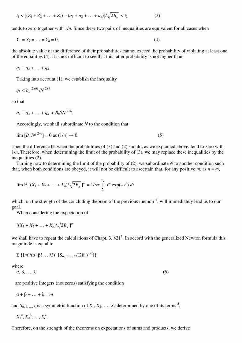
t1 < [(Z1 + Z2 + … + Zn) – (a1 + a2 + … + an)]/ nB2 < t2 (3)

tends to zero together with 1/n. Since these two pairs of inequalities are equivalent for all cases when Y1 = Y2 = … = Yn = 0, (4) the absolute value of the difference of their probabilities cannot exceed the probability of violating at least one of the equalities (4). It is not difficult to see that this latter probability is not higher than q1 + q2 + … + qn. Taking into account (1), we establish the inequality qk < bk

(2+�) /N 2+� so that q1 + q2 + … + qn < Bn�/N 2+�. Accordingly, we shall subordinate N to the condition that lim [Bn�/N 2+�] = 0 as (1/n) � 0. (5) Then the difference between the probabilities of (3) and (2) should, as we explained above, tend to zero with 1/n. Therefore, when determining the limit of the probability of (3), we may replace these inequalities by the inequalities (2). Turning now to determining the limit of the probability of (2), we subordinate N to another condition such that, when both conditions are obeyed, it will not be difficult to ascertain that, for any positive m, as n = �,

lim E [(X1 + X2 + … + Xn)/ nB2 ]m = 1/�� �∞

∞−

tm exp(– t2) dt

which, on the strength of the concluding theorem of the previous memoir 6, will immediately lead us to our goal. When consideríng the expectation of

[(X1 + X2 + … + Xn)/ nB2 ]m

we shall have to repeat the calculations of Chapt. 3, §217. In accord with the generalized Newton formula this magnitude is equal to W {[m!/(�! X! … !!)] [S�, X, …, ! /(2Bn)

m/2]} where �, X, …, ! (6) are positive integers (not zeros) satisfying the condition � + X + … + ! = m and S�, X, …, ! is a symmetric function of X1, X2, …, Xn determined by one of its terms 8, X1

�, X2X, …, Xi

!. Therefore, on the strength of the theorems on expectations of sums and products, we derive

E [(X1 + X2 + … + Xn)/ nB2 ]m = W [m!/(�! X! … !!)] [G�, X, …, ! /(2Bn) m/2]

where G�, X, …, ! is the expectation of the sum S�, X, …, ! and is obtained by issuing from it and replacing the powers of X1, X2, …, Xn by the expectations of the same powers. Regarding the expression G�, X, …, ! /(2Bn)

m/2, we shall prove that, when N is appropriately chosen, it will tend to zero together with 1/n for any possible system of numbers (6) excepting the system � = X = … = ! = 2 (7) which is only possible for even values of m. [4]To attain our goal, let us now turn our attention to a simple inequality [|G�, X, ..., ! |/Bn

m/2] < [(c1(�) + c2

(�) + … + cn(�))/Bn

�/2] … [(c1

(!) + c2(!) + … + cn

(!) )/Bn!/2]

whose right side consists of factors of the type [c1

(e) + c2(e) + … + cn

(e)]/Bne/2 (8)

where e can take values 1, 2, 3, … On the strength of the inequality written above we may state that, for any set of numbers (6) not exclusively consisting of twos, the ratio G�, X, …, !/Bn

m/2 will certainly tend to zero together with 1/n if N is chosen in such a way that, for e = 1, 3, 4, 5, …, lim {[c1

(e) + c2(e) + … + cn

(e)]/Bne/2} = 0, n = �.

Concerning the expression [c1

(2) + c2(2) + … + cn

(2)]/Bn (9) it is easy to convince ourselves that, for the values of N obeying the condition ascertained above, it ought to tend to 1 as n increases unboundedly. Indeed, when comparing the equality ck

(2) + EYk2 = bk

with the inequality EYk

2 < bk (2+�)/N �

whose validity it is not difficult to ascertain, we obtain bk > ck

(2) > bk – bk (2+�)/N �

so that by summation we obtain inequalities 1 > {[c1

(2) + c2(2) + … + cn

(2)]/Bn} > 1 – Bn�/[BnAN �]. Now, the expression Bn�/[BnAN �] can be represented as a product of two factors, [Bn�/N

2+�] �/(2+�) and [Bn�/Bn1+�/2] 2/(2+�),

both of them tending, under our conditions, to zero together with 1/n. Neither is it difficult to convince ourselves in that the conditions, to which we subordinated N, are sufficient for the ratio

[c1(1) + c2

(1) + … + cn(1)]/ nB

to tend to zero with 1/n. This follows from the simple inequalities ck

(1) < E |Yk| and [W E|Yk|]2 < (q1 + q2 + … + qn) W E Yk

2 < Bn W qk. Turning now to the ratios (8) for e = 3, 4, 5, … we bear in mind the inequality ck

(e) < N e–2

bk and obtain, consequently, [c1

(e) + c2(e) + … + cn

(e)]/Bne/2 < (N

2/Bn) (e–2)/2. .

It follows that all the ratios (8) will certainly tend to zero together with 1/n if we subordinate N to the condition that (N2/Bn) � 0 with 1/n. This new condition can be fulfilled together with the earlier restriction (5). Indeed, if we suppose that N = (BnYBn�)

1/(4+�) (10) then both fractions, N2/Bn and Bn�/N 2+� , will be reduced to one and the same expression [Bn�/Bn

1+�/2] 2/(4+�), which, on the strength of one of the Liapunov’s conditions assumed by us, should tend to zero together with 1/n. [5] And so, assuming (10), we may state that the difference between the probabilities of the inequalities (3) and (2) will tend to zero together with 1/n; that the ratio (9) will at the same time tend to 1; and, finally, that all the terms of the sum W{[m!/(�! X! … !!)] [G�, X, …, !/(2Bn)

m/2]} =

E [(X1 + X2 + … + Xn)/ nB2 ]m

will tend to zero together with 1/n excepting the only one which is determined by the equalities (7) and is only included in the sum when m is even. And, when taking into account the simple inequality (ck

(2))� < N 2�–2

ck(2)

for � = 2, 3, 4, …, we can easily establish the inequality {[(ck

(2))� + … + (cn(2))�]/Bn

�} < (N 2/Bn)

�–1 (11) which shows that under our conditions all the ratios of the type comprising the left side of (11) also tend to zero together with 1/n. It follows that under the indicated conditions the expectation of any positive odd degree of the ratio

(X1 + X2 + … + Xn)/ nB2

should tend to zero with 1/n. If, however, m is even, then it is the two differences 9

E[(X1 + X2 + … + Xn)/ nB2 ]n – (m!/2m/2) [G2, 2, ..., 2/(2Bn) m/2],

{[c1

(2) + c2(2) + … + cn

(2)]/2Bn}m/2 – (m!/2) [G2, 2, …, 2/(2Bn)

m/2] that should tend to zero. For the second one this follows from the identity [c1

(2) + c2(2) + … + cn

(2)]/2Bn]m/2 =

W{[(m/2)!/[Z! [! … �!] [HZ, [, …, �/(2Bn)

m/2]} and the inequality HZ, [, …, � < {[c1

(2)]µ + … + [cn(2)]µ} … {[c1

(2)]� + … + [cn(2)]�}

where HZ, [, …, � is a symmetric function of c1

(2), c2(2), …, cn

(2) determined by one of its terms [c1

(2)]µ [c2(2)][ … [cj

(2)]�. Thus, for an odd m, as n = �

lim E [(X1 + X2 + … + Xn)/ nB2 ]m = 0 = (1/��) �∞

∞−

tm exp (– t2) dt

and, for an even m, the left side is equal to

{m!/[2m (m/2)! ��]} �∞

∞−

t m exp (– t2) dt

which immediately provides the formulated limit theorem. In a similar way it can also be established for some other cases. We note, following Liapunov’s example, that his conditions are fulfilled if the absolute values of all the differences (Zk – ak) do not exceed one and the same constant number, and if, at the same time, lim Bn = lim (b1 + b2 + … + bn) = + � as n � �. (12) Indeed, if, for all values of k, – L < Zk – ak < L where L > 0 is constant, then, for any � > 0 we have bk

(2+�) = E |Zk – ak| 2+� < L�Ybk

so that Bn�/Bn

1+�/2 < L�/Bn�/2

and, if Bn increases unboundedly with n, lim [Bn�/Bn

1+�/2] = 0 as n = �. And it is not difficult to see that the provided proof of the theorem on the limit of probability is essentially easier for these cases since the need to introduce an auxiliary number N and to separate all the values of (Zk –

ak) into two sets disappears. [6] If, however, the absolute values of the differences (Zk – ak) can be arbitrarily large, then (12) is not in itself sufficient for the theorem to persist. This is shown by the following example. Suppose that, for sufficiently large values of k, Zk can take three values, 0, (log k)µ, – (log k)µ with probabilities

1 – 2/k (log k)[, 1/k (log k)[ and 1/k (log k)[

respectively. Here, Z and [ are given positive numbers and 2Z – [ + 1 > 0. (13) For other values of k let Zk = 0 so that a certain number ko of the first terms of the sum Z1 + Z2 + … + Zn (14) vanishes. We have ak = 0 for all values of k; E |Zk|

i = 0 for k \ ko; E Zk

2 = bk = [2(log k) 2µ–[/k] for k > ko and, in general, for any positive number i, E |Zk|

i = [2 (log k) iµ–[/k] for k > ko. It follows that Bn = [2[log (ko + 1)]2µ–[/(ko + 1)] + ... + [2(log n ) 2µ–[/n], Bn� = {2[log (ko + 1)](2+�) µ–[/(ko + 1)} + ... + [2 (log n)(2+�) µ–[/n]. When comparing these last sums with the corresponding integrals, it is easy to see that the ratios Bn/(log n)2µ–[+1, Bn�/(log n)(2+�) µ–[+1 cannot either increase unboundedly or become arbitrarily small. Then the same two statements will be true with respect to Bn� (log n) (1–[)�/2/Bn

1+�/2 = [Bn�/(log n) (2+�)µ–[+1]/[Bn/(log n) 2µ–[+1]1+�/2. We immediately conclude that for [ < 1 the Liapunov condition lim [Bn�/Bn

1+�/2] = 0, n = � is fulfilled, and, consequently, that the theorem on the limit of probability is valid. On the contrary, for [ ] 1 the Liapunov condition is evidently not fulfilled. This, however, does not yet prove that the limit theorem is not applicable to our case since that condition was established as a sufficient rather than a necessary restriction. For [ > 1 and sufficiently large values of ko we can easily prove that the theorem is not applicable by considering the probability that the sum (14) is exactly equal to zero. Had the theorem persisted, this probability would have tended to zero with an unbounded increase in n. At the same time it is not difficult to see that the probability of violating this equality is not higher than the sum of the probabilities that 10 +kZ = ± [log (ko + 1)]µ, …, Zn = ± (log n)µ

which is a part of an infinite sum

ν)]1( )[log1(

2

00 ++ kk+ … +

ν)]( [log )(

2

00 ikik ++

and should therefore remain less than

1

0 ])[log1(

2−− νν k

(15)

however great is n. Therefore, when choosing ko so large that (15) is less than unity, we may state that the probability that the sum (14) is zero is always higher than

1 – 1

0 ])[log1(

2−− νν k

> 0

and therefore does not tend to zero. For example, if [ = 2 and ko = 10, this probability is always higher than 1 – (2/log 10) > 1/8. We have thus ascertained that, if [ > 1, the theorem on the limit of probability is not applicable to the indicated cases. At the same time, on the strength of (13), condition (12) is fulfilled 10. Notes

Letter L stands for Linnik. 1. {Here and in some other cases below Markov refers to previous sections of his treatise [3, 1913].}

2. For this case, already De Moivre, in his Miscellanea analytica, in 1730, had outlined the proof that I attributed to Laplace. A.A.M. {Markov should have also referred to De Moivre’s “Method of approximating the sum of the terms of the binomial …” which first appeared in 1733 as a private publication.} 3. This contribution directly adjoins Markov’s previous memoir and for the first time presents the method of moments in a form allowing to prove the Liapunov “central limit theorem”. Liapunov justified this proposition by the method of characteristic functions which has the advantage that they exist for any random variable whereas the expectations of some of its powers do not always exist. Markov introduced “curtailed” random variables Xk, i.e., such functions of the initial random variables (Zk – ak) that their moments of any integer power do exist; and that under the Liapunov conditions the sum of these new variables has the same limiting distribution as the sum of the initial variables. Then, drawing on his previous memoir, Markov applied the method of moments to the sum (X1 + X2 + … + Xn). He concluded by providing an example in which the limit theorem did not take place with the Liapunov conditions, as is evident, being violated. L. {Linnik bears in mind Markov’s previous work [5]; actually, however, his contribution [1] should have been cited.} 4. {Here, Markov should have referred to his earlier version [4] of the present memoir; see [10, §5 of its second part].} 5. Suppose for the sake of simplicity that (Zk – ak) do not vanish and have a discrete distribution. Then P (Xk = Z – ak) = P (Zk – ak = Z – ak) if |Z – a| < N; P (Xk = 0) = P (|Zk – ak| ] N); P (Yk = Z – ak ) = P (Zk – ak = Z – ak); P (Yk = 0) = P (|Zk – ak| \ N) so that relation (1) {just below} follows immediately. The general case is treated similarly. L. 6. {Once more memoir [1] should have been cited.} 7. There, Markov proved the limit theorem under much more restrictive conditions. L. 8. {The series just below should apparently be written as a single term X1

� X2X …Xi

!.}

9. Chapter 3, §21. A.A.M. [ See Note 6.L.] 10. It is now possible to examine Markov’s example by means of the modern Lindeberg – Feller – Bernstein theorem which also allows to ascertain the unstudied case of [ = 1. Denote the law of distribution of (Zk – ak) by Fk(x) and assume that lim max (bk/Bn) = 0 as n � �, k @ n. Then

(1/Bn)�≤nk� x

2 dFk (x) � 0 as n � �, |�| > � nB

will be a necessary and sufficient condition for the applicability of the limit theorem for any fixed � > 0. For any such � and [ < 1, since

nB /[ln n]µ+(1–[)/2

is contained between positive constants, the inequality |Zk| > � nB is

impossible for sufficiently large values of n, and the condition is fulfilled. For [ > 1 we have, for a sufficiently small ^ > 0, k > e^ ln n, k @ n, and for a sufficiently large n

� x2 dFk(x) = bk, |�| > � nB , (1/Bn) �

≤ nei ln η

bi < Ko ^ 2µ–[+1,

(1/Bn)�≤nk� x

2 dFk (x) > 1/2, |�| > � nB . (*)

The condition is violated. Now, Ko, K1, … are positive constants. For [ = 1 and a given � we have for k > exp (K1 � ln n)

� x2 dFk (x) = bk , |�| > � nB , (1/Bn) �

≤ )ln( exp 1 nKi ε

bi < K2�2µ

and relation (*) persists. The condition is violated and the limit theorem is not applicable. L. References

A.A. Markov

[1] (1898). Sur les racines de l’équation … [2] (1899). The law of large numbers and the method of least squares. [3] (1900). ���������� ��� �� ��� (Calculus of Probability). [4] (1908). On some cases of the theorem on the limit of probability. [5] (1913). The Chebyshev inequalities and the main theorem. [6] (1951). ��������� ��� (Sel. Works).

Other Authors [7] Chebyshev, P.L. (1891). Sur deux théorèmes relatifs aux probabilités. [8] Liapunov, A.M. (1900). Sur une proposition de la théorie des probabilités.

[9] Liapunov, A.M. (1901). Nouvelle forme du théorème sur la limite de probabilité. [10] Linnik, Yu.V., Sapogov, N.A., Timofeev, V.N. (1951), An essay on Markov’s work in the theory of numbers and the theory of probability. In [6, pp. 614 – 640]. Translation of its second part: DHS 2656, 1999, pp. 205 – 218.

On the Work of Liapunov in the Theory of Probability

B.V. Gnedenko 1. General Information

Liapunov’s interest in probability was not more than an episode in his mathematical work. Indeed, the first of his pertinent writings appeared in 1900, and the last one in 1901. In all, he published five probability-theoretic papers [1 – 5] 1. One of these was of a polemic nature and the rest of them were devoted to solving a certain problem, viz.: Given, a sequence of mutually independent random variables �1, �2, …, �n, … having finite expectations and variances E�n = an, D�n = bn

2, Bn2 = b1

2 + b22 + … + bn

2. It is required to determine the most general conditions under which the laws of distribution for the sums sn = (1/Bn) [(�1 – a1) + (�2 – a2) + … + (�n – an)] tend to the normal law

U(x) = (1/ π2 ) �∞−

x

exp (–z2/2) dz.

Liapunov was prompted to examine this problem by preparing a course in the theory of probability with which the Physical and Mathematical Faculty of Kharkov University charged him at the very end of the last {of the 19th} century. He delivered that course during the academic years 1899 – 1900, 1900 – 1901, and 1901 – 1902. Already Chebyshev, in his lectures for the students of Petersburg University, indicated that studies of the problem formulated above were important. Liapunov attended these lectures in 1879 – 1880 and took them down in detail. Two years hence A.N. Krylov {a naval architect and applied mathematician} rewrote Liapunov’s notes and in 1936 they were published by the Soviet Academy of Sciences [14]. An outline of the limit theorem without its rigorous proof or a precise formulation of the result obtained is in §30 of this book (pp. 219 – 224). It ends on p. 224 with Chebyshev’s concluding words, as written down by Liapunov: Formula (38), that provides such a possibility was, however, derived in a

non-rigorous way. The lack of rigor in the derivation consisted in that we

made various assumptions without determining the boundary of the ensuing

errors. In its present state, mathematical analysis cannot derive this

boundary in any satisfying fashion.

These words undoubtedly induced Liapunov to busy himself with ascertaining the conditions for the applicability of the limit theorem. True, the investigations made by Markov [36; 37], Glaisher [24, p. 75; 25, p. 194] and Sleshinsky [44], with which Liapunov then acquainted himself, have also somewhat turned his attention to this problem. I noted that Liapunov had left a small number of publications on probability. However, only the depth and the importance of the obtained results and developed methods rather then the number of memoirs might serve as a proper estimate of a scholar’s scientific work. With respect to Liapunov, his contribution to probability had stood the test of time. The main fact, that he had discovered, was later called {by Polya, in 1920} the central

limit theorem of the theory of probability. Below, we shall also attempt to throw some light on his influence upon the direction of subsequent research. 2. On Previous Work The publication of Jakob Bernoulli’s celebrated work [7], where he had clearly formulated and proved the law of large numbers, led to natural problem of asymptotically estimating the probabilities of various deviations. De Moivre [18] had solved this problem for the simplest case of Bernoulli trials 2, i.e., for the case when p = q = 1/2. He thus introduced the normal law of distribution into science and it is obvious that the importance of his discovery for the further development of probability cannot be overestimated. Almost a century later Laplace [31] extended the De Moivre theorem up to its natural boundaries. Even more important for developing the methodology of this problem was perhaps Laplace’s attempt to study the possible asymptotic representations of the probabilities of events occasioned by a large number of independent causes. It seems that he first published some considerations about approaching the solution of this problem in 1781 [30]. Actually, with regard both to the formulation and methodology, the following Poisson theorem [42] adjoins the result obtained by De Moivre and Laplace: Suppose that a sequence of such independent trials 1, 2, … is carried out that in each of them a certain event can occur with probabilities p1, p2, … respectively. Denote the number of the occurrences of this event in n trials by µ. Then, as n � �, P {(1/Bn) [µ – (p1 + p2 + … + pn)] < x} � U(x), Bn

2 = p1(1 – p1) + p2(1 – p2) + … + pn(1 – pn). The interest in the normal distribution at the beginning of the 19th century had grown in connection with the appearance of Legendre’s [32] and Gauss’ [23] remarkable investigations devoted to the formulation and substantiation of the method of least squares 3. Their trains of thought were of a quite another nature and had no direct bearing on the theory of summing independent random variables; obliquely, however, they were very important by prompting Laplace to hasten the publication of his considerations on the methods of estimating some magnitude given the results of its independent observations. For us, his thoughts are very interesting because later on they have become the basis for substantiating the method of least squares. Laplace’s idea, that he nourished for almost thirty years, was this: The success of applying probability to various problems of natural sciences is founded on the fact that the sum total of a large number of random influences, with each of these having an insignificant effect as compared with all the other ones taken together, obeys some common general law. Below; I shall formulate the problems that Laplace had solved and describe his results. Bessel [11] indicated that the observations of the Greenwich astronomer Bradley had perfectly well fitted in with the normal law, and his explanation of this fact, which he expressed absolutely distinctly in 1838 [12], coincided with Laplace’s general idea. The observations of some magnitude obey the normal distribution because {as Bessel reasoned} their errors are occasioned by a large number of independent causes. For the case of measuring the zenith distance of a star by means of a meridian circle, Bessel listed 13 sources of random error. At the same time he indicated an example of errors of observation {of an error’s component} not obeying the normal distribution. Poincaré, in his course [41] in the theory of probability, adhered to the same approach for substantiating the normal law of distribution of observational errors. He twice described it in his Chapter 11. At first, at the end of §140, he stated that The error connected with the instrument is the sum total of a very large

number of errors independent one from another and such, that each of them

contributes only a small share of the general result; the total error follows

the Gauss law. Then, at the very beginning of §144, Poincaré concludes {after actually repeating himself}: “This, as it seems to me, is the best argument that might be put forward in favor of the Gauss law”. I ought to say, however, that all the ideas described above are only of a qualitative nature and should be mathematically justified. It is important to note that Laplace had advanced further than his contemporaries or

even subsequent scholars who worked during the first half of the 19th century. Not only had he formulated the idea that the error of observation was formed by summing up a large number of elementary errors; he also derived the distribution of such a sum as well as its asymptotic representation restricting his attention to the case of identically distributed terms taking integral values 1, 2, …, m with equal probabilities 1/m. 5 To solve his problem Laplace [31] applied the method of generating functions which he had earlier developed. And, to achieve his subsequent analytical transformations when solving stochastic problems, he denoted the argument t of the generating function by ei� thus introducing and making use of characteristic functions. Note also that, in accord with Laplace’s indication, Kramp, in 1796 [29], calculated the first table of the function U(x). I am unable to dwell here on the numerous subsequent writings devoted either to justifying the method of least squares and developing the theory of errors, or to the theory of summing independent random variables. I shall only mention Cauchy who systematically applied characteristic functions and showed that, when summing identically distributed independent random variables, the limiting distribution can be not only normal; it can belong to an entire class of distributions later called stable laws. The creation, in the 19th century, of the elements of statistical physics attached yet another dimension to, and stressed once again the fundamental importance of the normal law and the need of ascertaining the conditions under which it becomes the asymptotic distribution for sums of independent random variables. Chebyshev [15] made the first wide attempt in this direction. He did not persist in assuming that the random variables possessed any special properties and restricted his study by very general suppositions. The theorem that he formulated ran thus: If the expectations of variables u1, u2, … are zero, and the expectations of all of their powers are less in absolute value than some finite boundary, then, as n � �, the probability that the sum of n of these variables, divided by the square root of twice the sum of the expectations of their squares, is contained between some two boundaries t and t� tends to the integral

(1/��) �′t

t

exp (– x2) dx.

To prove this proposition, Chebyshev developed a very powerful method, later called the method of moments 6; its discovery constituted one of the greatest findings of the {mathematical} science of those days. However, the theorem as formulated above cannot be proved since its conditions are not stated clearly enough. First of all, it is not stipulated anywhere that the variables are mutually independent. Then, the demand that all the moments of all the variables be bounded by one and the same constant is too restrictive 7; in any case, it may be weakened by assuming that the moments of a certain order m are bounded by a constant C(m) depending only on m. Finally, the variance of the sum can increase with n not linearly, – not as is made use of in the proof. Once the necessary corrections are made, the Chebyshev proposition can be proved quite rigorously. The Chebyshev memoir also contains a draft estimate of how rapid is the convergence of the laws of distribution of the sums to the limiting law and an exposition of the idea of deriving asymptotic expansions of these laws of distribution in powers of 1/�n. The criticism of Chebyshev’s memoir as described above was in essence formulated by Markov in his letters to A.V. Vasiliev, a professor at Kazan University [37]. They also contained Markov’s positive contribution with a more rigorous and precise formulation of Chebyshev’s propositions, including his main lemmas. The same year Markov published a more detailed exposition of his results [36]. 3. The Subject-Matter of Liapunov’s Memoirs Liapunov, in a lengthy writing [1], after indicating some insufficiency of the reasoning and formulation in Chebyshev’s memoir [15], referred to the abovementioned Markov’s investigations. With respect to rigor and completeness he considered Markov’s exposition irreproachable, but he thought that Markov’s method of proof, connected with the development of a full theory, was involved and unwieldy. This fact inspired him to “revise the former methods”. We shall see, however, that he was able to succeed not only in developing a new method of proof, but also in discovering conditions final in some sense. a) The first formulation of the Liapunov theorem contained in the abovementioned work was in a certain way especially close to the Chebyshev proposition but demanded much less restrictions than the latter. Let mutually independent random variables �1, �2, …, �n, … have finite expectations ai = E�i, bi

2 = E (�i – ai)2, c i= E (|�i|)

3. Denote

Bn2 = b1

2 + b22 + … + bn

2, Ln3 = max ci, 1 ≤ i ≤ n

and assume that (Ln

2/Bn2)Yn2/3 � 0 as n � �.

Then, uniformly with respect to z1 and z2, P{ z1 < (1/Bn) [(�1 – a1) + (�2 – a2) + … + (�n – an)] < z2} � U(z2) – U(z1). Along with the proof itself, Liapunov rather thoroughly estimated the rapidity of the convergence to the normal law. I shall describe this point below. b) The second formulation. In his first note [2] Liapunov somewhat weakened the conditions of his theorem and had not anymore demanded that the terms have finite third moments. Denote a positive number not exceeding 1 by � and let Ln be defined by Ln

2+� = max E mod |xi|2+�, 1 ≤ i ≤ n.

If, for some �, (Ln

2/Bn2)Yn2/(2+ �) � 0 as n � �,

then, uniformly with respect to z1 and z2, as n � �, P (z1 < (1/Bn) [(�1 – a1) + (�2 – a2) + … + (�n – an)] < z2} �

(1/ π2 ) �2

1

z

z

exp (– x2/2) dx. (1)

c) The third and final formulation. This was published almost at the same time in a second note [3] and in memoir [4]. If for some positive � there exist finite moments di = E |�i – ai|

2+ � for all values of i, and if, as n � �, (d1 + d2 + … + dn)/Bn

2+ � � 0, then, uniformly with respect to z1 and z2, formula (1) takes place. In both his main memoirs Liapunov pays serious attention to the rapidity of the convergence of the laws of distribution of the sums sn to the limiting normal law. As far as the first memoir is concerned, I shall describe only one of its results: If the absolute third moments of the variables �i are bounded by a constant independent from i, then the difference n = sup|P(sn < x) – U(x)| x tends to vanish not slower than (ln n)/�n.

In the second memoir Liapunov [4] determined that n < cLn lnLn, Ln = (d1 + d2 + … + dn)/Bn

2+ �. There also he had derived the well-known inequalities connecting the moments of laws of distribution which found wide application both in probability and function theory. Here are his main general inequalities: Suppose that random variable � has an absolute moment of order k and let numbers k, m, n obey inequalities k > m > n

≥ 0. Then (E|�m|) k–n

< (E|�n|) k–m < (E|�k|) m–n

.

Of main importance for Liapunov’s own probability-theoretic investigations was a particular case of these inequalities; namely, if k > m > 0, (E|�m|) k < (E|�k|) m. For k = 3 and m = 2 Liapunov gave this inequality already in his memoir of 1900. Note that he derived all of them for the case in which the variable � takes a finite or a countable set of values; therefore, they concerned some infinite series with positive terms. However, it is not at all difficult to extend them onto the case of arbitrary distributions, and Liapunov himself saw this possibility as well. His special formulations were apparently occasioned by two circumstances, viz., by lack of convenient notation and the traditions concerning the form of writing that dated back to the outstanding mathematicians of former times. 4. The Liapunov Method We know that most important in science is not only the result obtained, but also the method applied for discovering it. Often the fact itself is soon derived as a corollary of more general findings made by others, whereas new ideas inherent in the method of proof become starting-points for many new results, achieved, furthermore, while investigating far away from the original problems. Concerning Liapunov’s studies, I ought to say that both his actual results and method of research developed by him have retained their importance until now. Liapunov himself gave much thought to developing new methods of proof. He thus followed his teacher who [13, p. 150] had stated that Whereas a theory has much to gain from new applications of an old

method, or from its further development, it acquires still more by

discovering new methods.

The first two pages of Liapunov’s memoir of 1900 are a brief essay on the research made by his predecessors with particular attention being given to evaluating their methods. He attached special significance to the application of the Dirichlet discontinuity factor made by the English astronomer Glaisher [24; 25]. At the same time, however, he noted that Glaisher’s method suffered from many shortcomings and cannot be directly applied for providing sufficiently general results. Liapunov also saw fit to mention a memoir by Sleshinsky [44] who had attempted to improve on the method of the discontinuity factor by applying Cauchy’s ideas but who

Introduced too restrictive assumptions and it is therefore impossible to

extend his analysis to more general cases.

In his §2 Liapunov [1] outlined his own method and indicated the difficulties that had to be surmounted. He assumed that random variables could only take a finite number of possible values. Introducing notation P (�i = xk) = fi (xk) he wrote down the probability of the inequalities g – h < �1 + �2 + … + �n < g + h

as a sum

� f1 (x1) f2 (x2) … fn (xn) extended over all the values of x1, x2, …, xn satisfying the inequalities g – h < x1 + x2 + … + xn < g + h.

By means of the Dirichlet integral

I = (2/�) �∞

0

[sin (ht/t)]cos st dt

where s = x1 + x2 + … + xn – g the probability sought can be written as

(2/�) �∞

0

[sin (ht/t)]Q dt (2)

where Q = � f1 (x1) f2 (x2) … fn (xn)cos st.

Under the conditions of the Liapunov theorem it is possible to prove that, as n � �,

lim (2/�) �τ

0

[sin (ht/t)]Q dt = (1/ π2 ) �2

1

z

z

exp (– z2) dz

where � is a positive number tending to zero with an increasing n in such a way that the magnitude L? n1/3 remains constant. Everything is

therefore reduced to proving that, as n # $,

lim �∞

τ

[sin (ht/t)]Q dt = 0,

and it is exactly here that the main difficulty is encountered.

We have assumed that the number of the possible values of each of the

variables is finite. Otherwise, as it occurs in the Glaisher analysis, yet a

new difficulty will present itself: the transformation necessary for obtaining

expression (2) can prove inadmissible.

Attempting to diminish these difficulties, I was obliged to begin by

introducing some assumptions which considerably narrowed the conditions

of the theorem. Then, however, I noted that these suppositions were not

necessary and that the difficulties can be sidestepped by means of an

artificial trick; namely, by considering, along with the variables �i, an

adequately defined supplementary variable.

Liapunov’s supplementary magnitude was independent of all the �i and distributed normally with variance 2_2 where _ was chosen depending on n and � but in such a manner that, as n # $,

�∞

τ

[sin (ht/t)]Q exp (–_2�2) dt # 0.

Thus, Liapunov was able to surmount the main difficulty by estimating the appropriate integral independently of the distributions of all the other terms by the magnitude written out just above. In §4, see his equality (9), Liapunov introduced functions that are now called characteristic. The supplementary term discussed above was necessary since the theory of characteristic functions was not yet developed. In proving his theorem, Liapunov had to overcome additional difficulties; more precisely, to prove, for his case, the theorems that now pertain to the theory of characteristic functions. In his §9 Liapunov showed that the initial restriction, connected with the supposed finiteness of the set of values taken by the separate terms, was not essential and that it was possible to disregard it. It is also noteworthy that at the beginning of his §4 Liapunov introduced the concept of distribution function 8 and indicated its elementary property writing it down as P (u ≤ � < v) = F (v) – F (u).

Liapunov fully explained his method in his first memoir. The second one had not demanded either essential changes of, or supplements to his method. Not more than natural and purely technical changes caused by a considerable generalization of the theorem were needed. His remark made there in §3 is of essential methodological importance. He noted that if his condition was fulfilled for some � > 0 then it held for any other �1 if only 0 < �1 < �. This fact was a simple corollary of the general Liapunov inequalities concerning absolute moments. Thus, Liapunov’s contributions considerably influenced the development of the theory of probability not only because they established one of its main propositions, but also since they fostered the growth of its new methods and (see below) ideas. 5. The Discussion with P.A. Nekrasov We have mentioned Liapunov’s polemic note [5]. It had not contained any new results being his rejoinder to Nekrasov’s rude attack [39] published soon after Liapunov’s studies had appeared in print. From the mathematical point of view, Nekrasov’s remarks were so indefinite, – and his conclusions so categorical, – that even now they can only stir up surprise and irritation. To give an idea about the style of his “criticism”, I venture to quote a rather long passage, highly typical of his entire note (and of many other of his contributions): his statements were categorical but not substantiated at all. {Gnedenko quotes [39, §1 and beginning of §2].} In his rejoinder, restrained in style but very sharp in essence, Liapunov indicated that Nekrasov had substantiated his conclusions only by very indefinite general reasoning, etc. {Gnedenko adduced three quotations from [5].} Liapunov’s reproof proved effective. In the concluding sections of his memoir [40], Nekrasov several times went back, although very indefinitely, on his criticism. Thus, on p. 441n he wrote: I ought to correct one indication in these critical remarks. I said that

Liapunov had applied the Dirichlet discontinuity factor. Instead, I should

have said that he had made use, in his method, of the same

disadvantageously lengthened path of integration that also plays its part

when this factor is applied. I believe, now also, that in every other respect

my critical remarks were correct, but I consider it necessary to supplement

them by positive comments.

We remember that Nekrasov’s other criticisms came to the impossibility of a simple formulation of the Liapunov theorem and to the persistence of the main shortcomings of the conclusions made by his predecessors. Nevertheless, Nekrasov (p. 442) now also declared something else: My remarks concerning the lack of rigor of their conclusions of course fall

away, but my criticisms of their incompleteness are still valid.

Somewhat below Nekrasov (p. 446) went even further by maintaining {in an unwieldy manner} that The Liapunov conditions coincide with those for one of the indications

sufficient for the fulfillment of the main conditions

derived in one of his (Nekrasov’s) early works. Thus, he recognized not only the irreproachability of the Liapunov result, but also the desirability of the statement that his own results were even more general. 6. The Direct Continuation of Liapunov’s Studies

Liapunov’s results gave rise to an enormous literature, to studies of considerable scientific importance. I am even unable to list all the papers directly or implicitly bearing on the described Liapunov’s memoirs and I restrict my exposition by a brief survey of a few main later works. It is necessary, above all, to mention Markov’s study {inserted in this book just above Gnedenko’s article} which was published as a supplement to his course [38]. In his introductory lines, Markov sufficiently clearly indicated that its appearance was caused by Liapunov’s memoirs. I think that his words are interesting and quote him accordingly {Gnedenko quotes the appropriate place from the beginning of Markov’s contribution.}

The method used by Markov consisted in curtailing the random variables and it is very often applied in the modern theory of probability. At the same time, it became a prototype of the concept of sequences of equivalent random variables. In 1922, the Finnish mathematician Lindeberg [35] had generalized Liapunov’s conditions of the central limit theorem, and, later on, Feller [22] proved that the Lindeberg conditions were, in a sense, not only sufficient but also necessary. In accord with these two studies we may now formulate the theorem on the convergence of the distribution functions of sums of independent terms to the normal law in the following way. It is sufficient for the distribution functions of sums sn to converge to the normal law U(x), that the Lindeberg conditions be fulfilled; namely, that for any � > 0 and n � �

(1/Bn2)��

=

n

k 1

(x – ak)2 dFk(x) � 0, |x – ak| > � Bn.

If, in addition, the pertinent terms are uniformly infinitely small, i.e., if, for any � > 0, as n � �, lim max P [|� k – a k| > � Bn] = 0, 1 ≤ k ≤ n, then the Lindeberg condition is also necessary for such convergence. It is interesting to note that Bernstein [9] had indicated that, in a sense, the Liapunov condition is also necessary. Suppose that it is fulfilled, then the central limit theorem is also true. And if the distribution functions of the sums converge to the normal law, and if, in addition, as n � �,

E|sn2+r| � (1/ π2 ) �

∞

∞−

|x2+r| exp (– x2/2) dx, 0 ≤ r ≤ �,

then the Liapunov condition of order � is necessarily fulfilled. Bernstein proved this theorem assuming that � > 1. In a previous work he [8] derived a sufficient condition for the convergence of the distribution functions of sums of independent terms to the normal law under very general assumptions that did not demand that the terms possessed moments of any order. Bernstein formulated this proposition in a note attached to the end of Chapter 1 (p. 74 of the Russian version) 9 since [9, p. 175] “this generalization is an almost obvious corollary of the Liapunov theorem”; however, he [9] exhaustively described it. Feller, in his abovementioned work [22], independently from Bernstein discovered the sufficiency and (for the case of small terms) necessity of the conditions indicated by Bernstein [8]. It should also be mentioned that in 1935, i.e., at the same time as Feller did, Khinchin [27] and Lévy [33], independently one from another, considered the case of identically distributed terms and obtained an elegant exhaustive result: It is necessary and sufficient for the sums

sn = [(� 1 + � 2 + … + � n) – An]/Bn (3)

of identically distributed independent random variables with appropriately chosen constants An and Bn > 0 to converge, as n � �, to the law U(x), that

x2� dF(z) = o { � z

2dF(z)}, x � �,

|z| ≥ x |z|< x

Cramér [16; 17], Esseen [20] and Studnev [45] specified the Liapunov estimates of the rapidity of the convergence of the distribution functions to the limiting law. In particular, Cramér showed that if the terms possessed third absolute moments, the constant C in the Liapunov estimate n < C�3nlg n (4) where

�3n =�=

n

i 1

E|� i – ai|3/Bn

3

can be equal to 3. For distribution functions F (x) of identically distributed terms whose characteristic functions f (t) fulfil condition lim sup |f (t)| < 1, | t | � � (5) and assuming that the third moments are finite, he proved that the inequality (4) can be replaced by a stronger condition n < M/�n. (6) Later Esseen [20] and Berry [10] discovered that (6) persists even if (3) is not satisfied. Esseen [21] recently showed that in the case under consideration

lim �n� (Un; U) ≤ K �3 where K = π26

103 +.

Equality is attained for the Bernoulli trials with steps

[( 10 – 2)/2], x = – [(4 – 10 )h/2]; [(4 – 10 )/2], x = [( 10 – 2)h/2] with h being any positive number. The natural question concerning the possible limiting distributions for sums of independent random variables was only formulated in full in the beginning of the 1930s. Bavli [6] and Khinchin [28] answered it, with the former, but not the latter, assuming that the terms possessed variances and Gnedenko and Doeblin studied an obvious problem about the conditions under which a limiting distribution can exist for consecutive sums derived from a given sequence of random variables. For a summary of all these studies see the monograph Gnedenko & Kolmogorov [26]. The work of Liapunov gave rise to numerous studies generalizing his propositions onto the summing of independent random vectors, and onto dependent terms; I shall not formulate the results obtained. It is now known that all the possible limiting distributions for the sums of independent random variables make up the extensive class of infinitely divisible distributions [26]. An appropriate natural question presents itself: how can it be explained that almost two centuries both the theory of probability proper, and its applications actually had to do only with the normal distribution? 10

Indeed, the other most important distribution, the Poisson law, was first indicated a hundred years later than the former, and its role in theoretical problems and applications was revealed completely enough only in our time. Cauchy discovered some stable distributions only in the middle of the 19th century, and until approximately the third decade of the next century they remained aside from the requirements of the theory of probability or statistics. Almost until the 1930s the normal law had been playing at least a dominant part in the theory of summing of random variables. Khinchin [28], also see [26, §26, Theorem 1], obtained a sufficiently complete answer. Its essence is that, for convergence to the normal law, only very general requirements, which barely restrict the specific character of the terms’ distributions, have to be fulfilled. Here is a rigorous formulation of his appropriate theorem: If a limiting distribution for the normed sums sn exists, then, for it to be normal, it is necessary and sufficient that the terms satisfy one single condition, viz., that, as n � �, P [sup|� k – ak| ≥ �Bn] � 0, 1 ≤ k ≤ n. It ought to be added that a similar, and even a somewhat more general formulation is in Lévy’s well-known book [34]. But, concerning his theorem, Khinchin [28, Note attached to §11] wrote: However, while basing my efforts on the outline indicated by Lévy, I was unable to

discover the proof of this proposition. Khinchin’s theorem shows that in an overwhelming majority of cases, and, in particular, for restricted random variables, the limiting distribution of the sums must be normal. For convergence to other distributions, some other conditions, which imply closeness of the pre-limiting distributions to the limiting law, have to be met.

Thus, we see that in summing independent random variables the normal distribution plays a special part and that this fact should have inevitably led to its consideration rather than to the application of the other possible limiting distributions. The Liapunov theorem very soon earned a conspicuous place in statistics, biology, physics, economics, and in the technological disciplines. A detailed description of its role in natural sciences and technology should comprise the subject of a special paper. In concluding, it remains to be said that Liapunov’s merits in probability are not exhausted by his proof of one of its main propositions. When appraising his contribution, it is necessary to allow for its influence on the development on this entire discipline during the last fifty years. Moreover, his impact persists. Suffice it to recall the principle of invariance as formulated by Donsker [19] or Prokhorov [43] for perceiving how the generalizations of Liapunov’s ideas lead to new and wider conclusions. Neither his result, nor the methods of proof developed by him have been relegated to the history of science. They are parts of a living organism of science, undergo essential changes and development, and find new possibilities for practical application. Notes 1. {There also existed a manuscript [5a] on the estimation of precision in the theory of errors written by Liapunov; it is now published.} 2. {The definitive source where De Moivre introduced the normal law is his Latin pamphlet of 1733 that he reprinted in English in the two later editions of his Doctrine of Chances. Yes, he had indeed restricted his attention to the particular case of p = q (in his notation, of a = b), but the title of his pamphlet contained the words binomial (a + b)n

and the text itself has the following phrase (p. 251 in the Doctrine’s edition of 1756): What we have said is also applicable to a Ratio of Inequality, as appears

from our 9th

Corollary.} 3. {Since Legendre had not at all introduced the normal law, Gauss’ merits should be emphasized. Then, the definitive Gaussian method of least squares did not depend on the normal (or any other) law of distribution.} 4. {Bessel had not claimed that Bradley’s observations perfectly well corresponded to the normal law. See my papers in vol. 49, 1995, Arch. Hist. Ex. Sci. and vol. 10, No. 1, 2000, Historia Scientiarum (Tokyo). The latter is a serious criticism of some of Bessel’s works.} 5. {Laplace also considered the case of arbitrary laws as well, see Mathematics of the 19

th century, vol. 1.

Editors, A.N. Kolmogorov & A.P. Youshkevich, pp. 224 – 225 of the chapter by Gnedenko & Sheynin. Basel, 1992.} 6. {This method is actually due to Bienaymé and Chebyshev. Below, at the end of §3, Gnedenko attributes to Liapunov some important inequalities. See C.C. Heyde & E. Seneta, Bienaymé. New York, 1977, pp. 111 – 112, who described Bienaymé’s relevant findings of 1840. 7. {This demand was possibly never made. Since Chebyshev sometimes wrongly used the singular form instead of the plural (see Note 3 to Liapunov’s paper in this book), readers could have misunderstood him.} 8. {Poisson hesitatingly introduced this concept.} 9. The main aim of this memoir [8] was to extend the Liapunov proposition onto sums of dependent random variables. 10. {This statement is too strong; Gnedenko himself, after a few lines, somewhat weakens it.} References

A.M. Liapunov 1 (1900), Sur une proposition de la théorie des probabilités. 2 (1901), Sur une théorème du calcul des probabilités. 3 (1901), Une proposition générale du calcul des probabilités. 4 (1901), Nouvelle forme du théorème sur la limite de probabilités. 5 (1901), An answer to P.A. Nekrasov. 5a (1975), On the Gauss formula, etc.

Other Authors

6. Bavli, G.M. (1936), Über einige Verallgemeinerungen der Grenzwertsätze der Wahrscheinlichkeitsrechnung. MS, vol. 1 (43), pp. 917 – 930. 7. Bernoulli, J. (1713, in Latin), Wahrscheinlichkeitsrechnung. Leipzig, 1899; Frankfurt/Main, 1999. 8. Bernstein, S.N. (1926), Sur l’extension du théorème limite du calcul des probabilités, etc. Math. Annalen, t. 97, pp. 1 – 59. 9. --- (1946), On a limit theorem, etc. In author’s �o������ � ������� (Works), vol. 4. N.p., 1964, pp. 434 – 447. (R) 10. Berry, A.C. (1941), The accuracy of the Gaussian approximation to the sum of independent variates. Trans. Amer. Math. Soc., vol. 49, pp. 122– 136. 11. Bessel, F.W. (1818), Fundamenta astronomiae. Königsberg. 12. --- (1838), Untersuchungen über die Wahrscheinlichkeit der Beobachtungsfehler. Abh., Bd. 2. Leipzig, 1876, pp. 372 – 391. 13. Chebyshev, P.L. (1856), Sur la construction des cartes, etc. 14. --- (1936), �� ��� ��� �� ��� (Theory of Probability). 15. --- (1891), Sur deux théorèmes relatifs aux probabilités. 16. Cramér, H. (1928), On the composition of elementary errors. Skand. Aktuarietidskr., t. 11, pp. 13 – 74 and 141 – 180. 17. --- (1937), Random Variables and Probability Distributions. Cambridge. Second ed., 1961. 18. De Moivre, A. (1730), Miscellanea analytica. Supplementum. London. 19. Donsker, M.D. (1951), An invariance principle for certain probability limit theorems. Mem. Amer. Math.

Soc., No. 6, pp. 1 – 12. 20. Esseen, C.G. (1945), Fourier analysis of distribution functions. Acta math., t. 77, pp. 1 – 125. 21. --- ( 1956), A moment inequality with an application to the central limit theorem. Skand. Aktuarietidskr., pp. 160 – 170. 22. Feller, W. (1935 – 1937), Über den zentralen Grenzwertsatz der Wahrscheinlichkeitsrechnung. Math. Z., Bd. 40, pp. 521 – 559; Bd. 42, pp. 301 – 312. 23. Gauss, C.F. (1871), Werke, Bd. 7. Gotha. 24. Glaisher, J.W.L. (1872), On the law of facility of errors of observations and on the method of least squares. Mem. Roy. Astron. Soc., vol. 39, pp. 75 – 124. 25. --- (1872), Remarks on certain portions of Laplace’s proof of the method of least squares. London,

Edinb. and Dublin Phil. Mag., 4th ser., vol. 43, pp. 194 – 201. 26. Gnedenko, B.V., Kolmogorov, A.N. (1949, in Russian), Grenzwertverteilungen von Summen

unabhängiger Zufallsgrössen. Berlin, 1959. 27. Kninchin, A.Ya. (1935), Sul dominio di attrazione della legge di Gauss. Giorn. Ist. Ital. Attuari, t. 6, pp. 371 – 393. 28. --- (1938), ���������� � ���� ��� ��� ����������� �������� ������� (Limit Theorems for Sums of Independent Random Variables). M. 29. Kramp, C. (1796), Analyse des refractions astronomiques et terrestres. Strassbourg. 30. Laplace, P.S. (1781), Sur les probabilités. Oeuvr. Compl., t. 9, Paris, 1893, pp. 383 – 485. 31. --- (1812), Théorie analytique des probabilités. Ibidem, t. 7. Paris, 1886. 32. Legendre, A.M. (1805), Nouvelles méthodes pour la détermination des orbites des comètes. Paris. 33. Lévy, P. (1935), Propriétés asymptotiques des sommes de variables aléatoires indépendantes ou enchaînées. J. math. pures et appl., sér. 7, t. 14, pp. 347 – 402. 34. --- (1937), Théorie de l’addition des variables aléatoires. Paris. 35. Lindeberg, J.W. (1922), Eine neue Herleitung des Exponentialgesetzes in der Wahrscheinlichkeitsrechnung. Math. Z., Bd. 15, pp. 211 – 225. 36. Markov, A.A. (1898), Sur les racines de l’équation, etc. 37. --- (1899), The law of large numbers and the method of least squares. 38. --- (1900), ���������� ��� �� ��� (Calculus of Probability). Third ed., 1913. 39. Nekrasov, P.A. (1901), Concerning a simplest theorem on the probability, etc. translated in this book. 40. --- (1900 – 1902), New principles of the doctrine of probabilities, etc. 41. Poincaré, H. (1912), Calcul des probabilités. Paris, second ed. 42. Poisson, S.D. (1837), Recherches sur la probabilité des jugements, etc. Paris. 43. Prokhorov, Yu.V. (1953), Distribution of probabilities in functional spaces. Uspekhi Matematich. Nauk, vol. 8, No. 3 (55), pp. 165 – 167. (R)

44. Sleshinsky, I.V. (1892), On the theory of the method of least squares. Zapiski Novoross. Obshchestvo

Estestvoispytatelei, Matematich. Otdelenie, vol. 14, pp. 201 – 264. (R) 45. Studnev, Yu.P. (1958), On a specification of the Liapunov theorem. Doklady Akad. Nauk Ukrainy, No. 2. (R)

Index of Names

Not covering either the Bibliography or the references to separate papers. Chebyshev, Liapunov, Markov and

Nekrasov are not included

Explanation The bold numbers are those of the items in the Contents. Notation such as i.1; j.3Add; k.f; m.n denotes §1 in item i; §3, Addendum in item j; Foreword to item k; and Notes to item m. Finally, F stands for Foreword to the book itself. Andreev, K.A. 6f; 9.16n; 13n; 14.2 Alekseev, V.G. 13.5 Aristotle F

Bavli, G.M. 16.6 Bayes, T. 7.6; 7n Bekhterev, V.M. 9.15 Bernoulli, D. 12.4; 12n Bernoulli, J. 1.1 – 1.4; 7.2; 7.5; 13.2, 15.1, 16.2, 16.6 Bernoulli, N. 12n Bernstein, S.N. 15n, 16.6 Berry, J.B. 16.6 Bertrand, J. 7n; 13.3 Bessel, F.W. 9.12n, 16.2, 16n Bienaymé, I.J. 7.2; 7.3; 7.5; 8; 9.3; 10.1; 13.2, 16n Bobylev, D.K. 9.17 Bortkiewicz, L. von (Bortkevich, V.I.) F

Bradley, J. 16.2, 16n Briggs, H. 7.2 Buckle, H.T. 12.2; 12.3 Buffon, G.L.L. 12.4 Bugaev, N.V. 9.17; 9.17n; 13.2 Bukreev, B.Ya. 9.8; 9.12 Cauchy, A.L. 2; 7.2; 7.3; 10.1; 13.2; 13n,16.2, 16.4, 16.6 Charlier, C.V.L. 7n Chelpanov, G.I. 13.2 Chirikov, M.V. F; 9.16n; 13n Chuprov, A.A. F Comte, A. 12.2 Cramer, G. 12n Cramér, H. 16.6 Czuber, E. 12.1 Darboux, G. 2 Davidov, A.Yu. 7.3; 7n De Moivre, A. 15n, 16.2, 16n Descartes, R. F Dirichlet, P.G.L. 5.1; 5.4; 6.2; 7.3; 7n; 10.1 Dmitriev, A.L. 12f; 14.3f Donsker, M.D. 16.6 Dostoevsky, F.M. 12.1 Dubrovin, N.F. F; 9.8; 9.9; 9.11 Engels, F. 12.3

Esseen, C.G. 16.6 Euler, L. 7.1; 13.2 Feller, W. 15n, 16.6 Fick, L. 12.4 Florensky, P.A. F Florov, P.S. 13.1; 13.4 Fouillée, A.J.E. 12n Gauss, C.F. 7.4; 9.12n; 10f; 10.1; 10.3; 11.2, 16.2, 16n Glaisher, J.W.L. 16.1, 16.4 Gnedenko, B.V. F, 6n; 7n Gogol, N.V. 12.1 Goncharov, I.A. 12.1 Gordevsky, D.Z. 14.2 Grave, D.A. 14.7 Haeckel, E. 13.2 Hegel, G.W.F. 12.3 Heyde, C.C. 16n Imshenetsky, V.E. 9.17; 13.2 Jordan, C. 13.3 Kant, I. F Karpenko, B.I. 12f Khinchin, A.Ya. 16.6 Khrushchev, P.D. 7.4 Kolmogorov, A.N. 16.6, 16n Kovalevskaia, S.V. 9.10n; 9.13n Kramp, C. 16.2 Krylov, A.N. 9.17, 16.1 Lagrange, J.L. 1.3; 7.1; 7.6; 13.2; 13.3; 13n Lakhtin, L.K. 7.4 Laplace, P.S. F; 2; 4.5; 4.6; 5.1; 5.2; 7.1; 7.3 – 7.6; 8; 9.2; 10f; 10.1; 10.3; 11.2; 12.2; 12.9; 13.2, 15.1, 15n, 16.2 Lappo-Danilevsky, A.S. 12.2 Laurent, H. 4.4; 4n; 7.3; 9.3, 9.5; 9.6; 10.1; 10.3Add Legendre, A.M. 10f; 10.1, 16.2, 16n Leibniz, G.W. F; 12.2 Lévy, P. 16.6 Lindeberg, J.W. 15n, 16.6 Linnik, Yu.V. 15f, 15n Loria 12.3 Marat, J.P. 12.8 Marx, K. 12.3 Mill, J.S. F Newton, I. 13.4 Oettingen, A., von 12.1 Oldenburg, S.F. 9.17 Ozerov 14.3 Pearson, K. 7.4; 7.6; 9.16n 13.2, 13.4; 14.4 Plato F

Poincaré, H. 9.16, 16.2 Poisson, S.D. 1.1; 3; 7.1; 7.3; 7.5; 7n, 16.2, 16.6 Posse, K.A. 9.13; 9.17; 13.1; 13.2; 13.4; 13n Prokhorov, Yu.V. 16.6 Pushkin, A.S. 12.1 Quetelet, A. 1.2; 1n; 12.1 – 12.3; 12.5; 12.8 Radlov, E.L. 14.6 Robespierre, M.Y., de 12.8

Romanov, K.K. 9.9; 9.11 Rousseau, J.J. 12.8 Seneta, E. F; 6n, 16n Sintsov, D.M. 14.8 Sleshinsky, I.V. 7.3; 10.1, 16.1, 16.4 Slutsky, E.E. 14.4 Soloviev, A.D. F, 1.3 Soloviev, V.S. F; 12n Sonin, N.Ya. 14.3f Steklov, V.A. 6f; 9.17; 14.1 Stirling, J. 1.3; 1.4 Studnev, Yu.P. 16.6 Süssmilch, J.P. 12.1 Tikhomandritsky, M.A. 11.1; 11.4n Todhunter, I. 7.6 Tolstoy, L.N. 12.1; 12.5 Torquemada, T. 12.8 Tsinger, N.Ya. 7n; 9.17 Tsinger, V.Ya. 10.1 Tsykalo, A.L. 6f; 9.10n Umov, N.A. 9.16n Usov, N.A. 10n Vasiliev, A.V. 9.8Add; 9n; 9.12; 9.15; 13.4, 16.2 Vinogradov, P.G. 12.6 Wagner, Ad. 12.3 Wieser, F. von 12.4 Yanson, Yu.E. 12.1; 12.2 Yanzhul, I.I. 14.3 Yarochenko, S.P. 10.3Add; 11.1; 11.3; 11.4 Youshkevich, A.P. 16n Zenon Eleates 13.3 Zhukovsky, N.E. F