Alma Mater StudiorumUniversita degli Studi di Bologna

Facolta di Scienze Matematiche, Fisiche e Naturali

Corso di Laurea in Matematica

Tesi di Laurea in Geometria III

Knot Theory and its

applications

Candidato: Relatore:

Martina Patone Chiar.ma Prof. Rita Fioresi

Anno Accademico 2010/2011 - Sessione II

.

.

Contents

Introduction 11

1 History of Knot Theory 15

1 The Firsts Discoveries . . . . . . . . . . . . . . . . . . . . . . 15

2 Physic’s interest in knot theory . . . . . . . . . . . . . . . . . 19

3 The modern knot theory . . . . . . . . . . . . . . . . . . . . . 24

2 Knot invariants 27

1 Basic concepts . . . . . . . . . . . . . . . . . . . . . . . . . . . 27

2 Classical knot invariants . . . . . . . . . . . . . . . . . . . . . 28

2.1 The Reidemeister moves . . . . . . . . . . . . . . . . . 29

2.2 The minimum number of crossing points . . . . . . . . 30

2.3 The bridge number . . . . . . . . . . . . . . . . . . . . 31

2.4 The linking number . . . . . . . . . . . . . . . . . . . . 33

2.5 The tricolorability . . . . . . . . . . . . . . . . . . . . 35

3 Seifert matrix and its invariants . . . . . . . . . . . . . . . . . 38

3.1 Seifert matrix . . . . . . . . . . . . . . . . . . . . . . . 38

3.2 The Alexander polynomial . . . . . . . . . . . . . . . . 44

3.3 The Alexander-Conway polynomial . . . . . . . . . . . 46

4 The Jones revolution . . . . . . . . . . . . . . . . . . . . . . . 50

4.1 Braids theory . . . . . . . . . . . . . . . . . . . . . . . 50

4.2 The Jones polynomial . . . . . . . . . . . . . . . . . . 58

5 The Kauffman polynomial . . . . . . . . . . . . . . . . . . . . 63

3 Knot theory: Application 69

1 Knot theory in chemistry . . . . . . . . . . . . . . . . . . . . . 69

4 Contents

1.1 The Molecular chirality . . . . . . . . . . . . . . . . . . 69

1.2 Graphs . . . . . . . . . . . . . . . . . . . . . . . . . . . 73

1.3 Establishing the topological chirality of a molecule . . . 78

2 Knots and Physics . . . . . . . . . . . . . . . . . . . . . . . . 83

2.1 The Yang Baxter equation and knots invariants . . . . 84

3 Knots and biology . . . . . . . . . . . . . . . . . . . . . . . . 86

3.1 Tangles and 4-Plats . . . . . . . . . . . . . . . . . . . . 87

3.2 The site-specific recombination . . . . . . . . . . . . . 91

3.3 The tangle method for site-specific recombination . . . 92

Bibliography 96

List of Figures

1 Wolfagang Haken’s gordian knot . . . . . . . . . . . . . . . . . 11

1.1 Stamp seal (1700 BC) . . . . . . . . . . . . . . . . . . . . . . 15

1.2 The Gauss’ scheme for the trefoil knot . . . . . . . . . . . . . 17

1.3 The Hopf link . . . . . . . . . . . . . . . . . . . . . . . . . . . 18

1.4 The crossings signs . . . . . . . . . . . . . . . . . . . . . . . . 19

1.5 Chirality of the trefoil . . . . . . . . . . . . . . . . . . . . . . 21

1.6 Maxwell’s scheme . . . . . . . . . . . . . . . . . . . . . . . . . 21

1.7 The flype move . . . . . . . . . . . . . . . . . . . . . . . . . . 23

1.8 The Reidemeister moves . . . . . . . . . . . . . . . . . . . . . 25

2.1 Connected sum of two knots . . . . . . . . . . . . . . . . . . . 28

2.2 Reidemeister moves . . . . . . . . . . . . . . . . . . . . . . . . 29

2.3 Different diagrams with different crossing points . . . . . . . . 30

2.4 The bridges of the trefoil knot . . . . . . . . . . . . . . . . . . 31

2.5 The bridges number of the trefoil knot . . . . . . . . . . . . . 32

2.6 The Whitehead link and the Borromean rings . . . . . . . . . 33

2.7 The unlink and the Hopf link . . . . . . . . . . . . . . . . . . 33

2.8 Computing linking number. . . . . . . . . . . . . . . . . . . . 34

2.9 The second Reidemeister move does not effect linking number. 34

2.10 The third Reidemeister move does not effect linking number. . 35

2.11 Tricolorability of the trefoil . . . . . . . . . . . . . . . . . . . 35

2.12 The first Reidemeister move preserves tricolorability. . . . . . 36

2.13 The second Reidemeister move preserves tricolorability. . . . . 36

2.14 The third Reidemeister move preserves tricolorability. . . . . . 37

2.15 The un-tricolorability of the figure-eight knot . . . . . . . . . 38

2.16 Splicing of a knot . . . . . . . . . . . . . . . . . . . . . . . . . 38

6 List of Figures

2.17 Figure eight seifert surface . . . . . . . . . . . . . . . . . . . . 39

2.18 Positive and negative twist . . . . . . . . . . . . . . . . . . . . 39

2.19 Closed curves in the Seifert surface of the figure-eight knot. . . 42

2.20 The Seifert surface with two closed curves. . . . . . . . . . . . 42

2.21 The Seifert surface of the trefoil knot . . . . . . . . . . . . . . 46

2.22 The closed curves of the trefoil knot 1 . . . . . . . . . . . . . . 46

2.23 The closed curves in the trefoil knot 2 . . . . . . . . . . . . . . 47

2.24 Skein diagrams . . . . . . . . . . . . . . . . . . . . . . . . . . 47

2.25 Skein diagrams for the unlink . . . . . . . . . . . . . . . . . . 48

2.26 Skein diagrams for the trefoil knot . . . . . . . . . . . . . . . . 48

2.27 Skein diagrams for the figure-eight knot . . . . . . . . . . . . . 49

2.28 Example of braid . . . . . . . . . . . . . . . . . . . . . . . . . 50

2.29 Trivial braid . . . . . . . . . . . . . . . . . . . . . . . . . . . . 50

2.30 Two equivalent braids . . . . . . . . . . . . . . . . . . . . . . 51

2.31 The product of two braids . . . . . . . . . . . . . . . . . . . . 52

2.32 The product of braids is not commutative . . . . . . . . . . . 52

2.33 The product of braids is associative . . . . . . . . . . . . . . . 53

2.34 The unit of a braid group . . . . . . . . . . . . . . . . . . . . 53

2.35 The inverse of a braid group . . . . . . . . . . . . . . . . . . . 54

2.36 The generators of the braid group . . . . . . . . . . . . . . . . 54

2.37 The generators of a braid . . . . . . . . . . . . . . . . . . . . . 55

2.38 Two equivalent braids 1 . . . . . . . . . . . . . . . . . . . . . 55

2.39 Two equivalent braids 2 . . . . . . . . . . . . . . . . . . . . . 56

2.40 The closure of braid . . . . . . . . . . . . . . . . . . . . . . . . 56

2.41 An algorithm for creating center of knots. . . . . . . . . . . . 57

2.42 An algorithm for creating center of knots. . . . . . . . . . . . 57

2.43 Braids and knots . . . . . . . . . . . . . . . . . . . . . . . . . 58

2.44 The Markov moves . . . . . . . . . . . . . . . . . . . . . . . . 58

2.45 The Jones polynomial of the trefoil knot . . . . . . . . . . . . 61

2.46 The Jones polynomial of the figure-eight knot . . . . . . . . . 61

2.47 Nonequivalent knots with the same Jones polynomial . . . . . 62

2.48 Splicing of a knot . . . . . . . . . . . . . . . . . . . . . . . . . 63

2.49 Two equivalent trivial knot . . . . . . . . . . . . . . . . . . . . 64

2.50 Applying the first Reidemeister move to a knot. . . . . . . . . 65

List of Figures 7

2.51 Skein diagram of the unknot . . . . . . . . . . . . . . . . . . . 66

2.52 Skein diagram of the Hopf link . . . . . . . . . . . . . . . . . . 66

3.1 A chiral molecule . . . . . . . . . . . . . . . . . . . . . . . . . 71

3.2 A molecule chemically achiral but geometrically chiral . . . . . 71

3.3 A topological rubber glove molecule . . . . . . . . . . . . . . . 72

3.4 Geometric representation of a graph . . . . . . . . . . . . . . . 74

3.5 The following graphs are isomorphic. Indeed, the required iso-

morphism is given by v1 → 1, v2 → 3, v3 → 4, v4 → 2, v5 → 5. . 74

3.6 Examples of planar graphs . . . . . . . . . . . . . . . . . . . . 75

3.7 complete graph Kn, n = 1, 2, 3, 4. . . . . . . . . . . . . . . . . 75

3.8 A pentagon . . . . . . . . . . . . . . . . . . . . . . . . . . . . 76

3.9 Make an edge between a and c. . . . . . . . . . . . . . . . . . 76

3.10 The edge betwenn b and d cannot be added it inside (since

it would cross a, c) nor can we add it outside (since it would

cross c, e). . . . . . . . . . . . . . . . . . . . . . . . . . . . . . 77

3.11 The complete bipartite graph K3,3 . . . . . . . . . . . . . . . . 77

3.12 A molecular Mobius ladder . . . . . . . . . . . . . . . . . . . . 78

3.13 Two molecules and their Jones polynomial . . . . . . . . . . . 79

3.14 We color the rings of a Mobius ladder and then deform the

sides of the ladder into a planar circle. . . . . . . . . . . . . . 79

3.15 The 2-fold branched cover of a Mobius ladder, branched over

the side of the ladder. The vertical descending order of the

rungs is: dashed, light grey, dotted, dashed, light grey, dotted. 80

3.16 Triple layered naphthalenophane (TLN) . . . . . . . . . . . . 80

3.17 Triple layered naphthalenophane (TLN) . . . . . . . . . . . . 81

3.18 K5 and K3,3 . . . . . . . . . . . . . . . . . . . . . . . . . . . . 81

3.19 The ferrocenophane molecule . . . . . . . . . . . . . . . . . . 82

3.20 The ferrocenophane molecule . . . . . . . . . . . . . . . . . . 82

3.21 The DNA . . . . . . . . . . . . . . . . . . . . . . . . . . . . . 86

3.22 Example of tangles: a. rational, b. trivial, c. prime, d.locally

knotted . . . . . . . . . . . . . . . . . . . . . . . . . . . . . . 87

3.23 Addition between two tangles . . . . . . . . . . . . . . . . . . 88

3.24 Numerator and Denominator operations . . . . . . . . . . . . 88

3.25 The Hopf link as the numerator of a tangle . . . . . . . . . . . 88

8 List of Figures

3.26 Four exceptional rational tangles in the Conway symbols . . . 90

3.27 4-plat < 2, 1, 1 > . . . . . . . . . . . . . . . . . . . . . . . . . 90

3.28 A simple site-specific recombination. . . . . . . . . . . . . . . 92

3.29 The synaptic complex as a result of a tangles operation. . . . . 92

3.30 N(S +R) =the product. . . . . . . . . . . . . . . . . . . . . . 93

3.31 N(S + E) = the substrate. . . . . . . . . . . . . . . . . . . . . 93

Introduzione

Questa tesi si occupera dare una introduzione alla teoria dei nodi. Nei tre

capitoli verranno presi in considerazione tre aspetti. Si descrivera come la

teoria dei nodi si sia sviluppata nel corso degli anni in relazione alle diverse

scoperte scientifiche avvenute. Si potr quindi subito avere una idea di come

questa teoria sia estremamente connessa a diverse altre. Nel secondo capitolo

ci si occuper degli aspetti pi formali di questa teoria. Si introdurra il concetto

di nodi equivalenti e di invariante dei nodi. Si definiranno diversi invarianti,

dai piu elementari, le mosse di Reidemeister, il numero di incroci e la tri-

colorabilita, fino ai polinomi invarianti, tra cui il polinomio di Alexander, il

polinomio di Jones e quello di Kauffmann. Infine si spiegheranno alcune ap-

plicazioni della teoria dei nodi in chimica, fisica e biologia. Sulla chimica, si

definira la chiralita molecolare e si mostrera come la chiralita dei nodi possa

essere utile nel determinare quella molecolare. In campo fisico, si mostrera la

relazione che esiste tra l’equazione di Yang-Baxter e i nodi. E in conclusione

si mostrera come modellare un importante processo biologico, la recombi-

nazione del DNA, grazie alla teoria dei nodi.

Introduction

“When Alexander reached Gordium, he was seized with a longing to ascend to the

acropolis, where the palace of Gordius and his son Midas was situated, and to see

Gordius wagon and the knot of the wagons yoke:. Over and above this there was a

legend about the wagon, that anyone who untied the knot of the yoke would rule

Asia. The knot was of cornel bark, and you could not see where it began or ended.

Alexander was unable to find how to untie the knot but unwilling to leave it tied,

in case this caused a disturbance among the masses; some say that he struck it

with his sword, cut the knot, and said it was now untied.”

- Lucius Flavius Arrianus, ”Anabasi Alexandri”, Book II-

Figure 1: Wolfagang Haken’s gordian knot.

Alexander unties the gordian knot, according to the legend, cutting it. The

history wants him to became the ruler of Asia, but mathematically speaking,

Alexander have never solved that enigma. In fact a knot can be untied if it

can be deformed smoothly into a circle, that is without any cut!

12 Introduction

Given a knot, is it possible to have different deformation of the same.

This give raise to a mathematical problem: to state if, among all the different

deformations of a given knot, is it possible to find an unknotted loop.

That is the central idea of the Knots Theory. The main problem of this

subject is in fact, given two different knot, to state if they are (topologically)

equivalent, isotopic, that is if they can be smoothly deformed one into the

other. In this sense, a loop is unknotted if is equivalent to a circle in the

plane. Different way to the approach that problem were used during the past

years. The first idea was to consider the knot as 1-surface and studying it

through the property of their complement in a 3-dimensional space.

This method is the one that give birth to the topology. The term “topology”

was, in fact, coined by Johann Listing in the 1848, in order to describe a

subject that was interested in the qualitative property of an object, instead

than in the quantitative property.

Let’s take a step back. Leibniz wrote in 1679:

I consider that we need yet another kind of analysis,. . . which

deals directly with position

and he called it “geometry of position”(geometria situs). That is, the history

of the knot theory is also the history of the development of this new geometry

theorized by Leibniz.

In this dissertation, we are going to give a brief introduction of knot theory,

looking at different aspects.

In the first chapter, we will see how the research on this subject changed

during the time. Starting from the prehistorical discovers of knots, we will

see how the interest in this field increase whit the idea that the matter is

made by vortex. This idea brought several scientists to be interested in knots:

Tait, Maxwell, Thompson and Kirkman among the others.

The last section is about the modern knot theory. In particular about the

first main breakdown due to Alexander and Reidemeister’s discoveries of new

invariants and the second one due to Jones and its new polynomial.

Introduction 13

In the second chapter we will consider knot as curves in R3 and we will be

interested in their mathematical properties. In this chapter we investigate a

way for determining whether or not two knot are equivalent. Different knots

invariants are going to be introduced.

The first section will give us some basic concept about knot theory.

The second section is dedicated to the classical knots invariant: the Reide-

meister moves, the bridge number, the linking number and the tricolorability.

In the third section the Seifert matrix is introduce, in order to compute the

Alexander polynomial and Alexander-Conway polynomial.

The fourth section is about the Jones polynomial. And for computing it an

introduction on braids groups is required. The last invariant to be introduced

is the Kauffman polynomial.

In the last chapter we will show how knot theory influenced others discipline:

chemistry, physics and biology.

Chapter 1

History of Knot Theory

My soul is an amphicheiral knot Upon a liq-

uid vortex wrought By Intellect in the Un-

seen residing, While thou dost like a convict

sit With marlinspike untwisting it Only to

find my knottiness abiding

James Clerk Maxwell, A paradoxical ode

1 The Firsts Discoveries

Knots have been center of interest for humans beings since the prehistory. The

first example we have is a seal found in Anatolia, dated 1700 B.C., represented

braids and knots. However the earliest discovery of knots is attributed to a

Greek physician named Heraklas, who lived during the first century A.D.

Figure 1.1: Stamp seal, about 1700 BC (the British Museum).

In fact he wrote an essay on surgeons slings in which he explains eighteen

16 History of Knot Theory

ways to tie orthopedic slings. Even if it was not properly knot theory, it

should be taken as the first example of knot theory’s application we have in

the scientific literature. Although we could think of knot theory as a ancient

discipline, in the mathematical scene is quite a new arrival.

In a letter to Christian Huygens (1629-1695), written in 1679 [9], Gottfried

Willhelm Leibniz, German philosopher and mathematician wrote:

I am not content with algebra, in that it yields neither the short-

est proofs nor the most beautiful construction of geometry. Con-

sequently, in view of this, I consider that we need yet another kind

of analysis, geometric or linear, which deal directly with position,

as algebra deals with magnitude.

With those word Leibniz laid the basis for a new science that he called

geometria situs, geometry of position, and that is now known as topology.

The first example of Leibniz’s new conception of geometry was given by

Leonard Euler (1707-1783). Solving the bridges of Konigsberg problem, Euler

did not worry about the exact position of the bridges, instead he recognized

that the key information was to understand which properties derive from

their reciprocal position.

He wrote in his paper Solutio problematis ad geometriam situs pertinentis [4],

1736 :

The branch of geometry that deals with magnitudes has been zeal-

ously studied throughout the past, but there is another branch that

has been almost unknown up to now; Leibniz spoke of it first, call-

ing it the ”geometry of position”. This branch of geometry deals

with relations dependent on position: it does not take magnitudes

into considerations, nor does it involve calculation with quantities.

But as yet no satisfactory definition has been given of the prob-

lems that belongs to this geometry of position or of the method to

be used in solving them.

But only in the 1771, for the first time, knot theory was mentioned as a field of

studies by Alexander-Theophile Vandermonde (1735-1796). He studied braids

and knots as examples of this new science of position envisioned by Leibniz.

1.1 The Firsts Discoveries 17

He wrote in his paper Remarques sur les problmes de situation (Remarks on

problems of position) [20]:

Whatever the twist and turns of a system of threads in space,

one can always obtain an expression for the calculation of its

dimensions, but this expression will be of little use in practice.

The craftsman who fashions a braid, a net, or some knots will be

concerned, not with questions of measurement, but with those of

position: what he sees there is the manner in which the threads

are interlaced.

One of the oldest notes by Gauss to be found among his papers

is a sheet of paper with the date 1794. It bears the heading “A

collection of knots” and contains thirteen neatly sketched views

of knots with English names written beside them . . . With it are

two additional pieces of paper with sketches of knots. One is dated

1819: the other is much later, . . . [16]

Carl Friedrich Gauss’ studies were essential for the creation of the knot the-

ory.

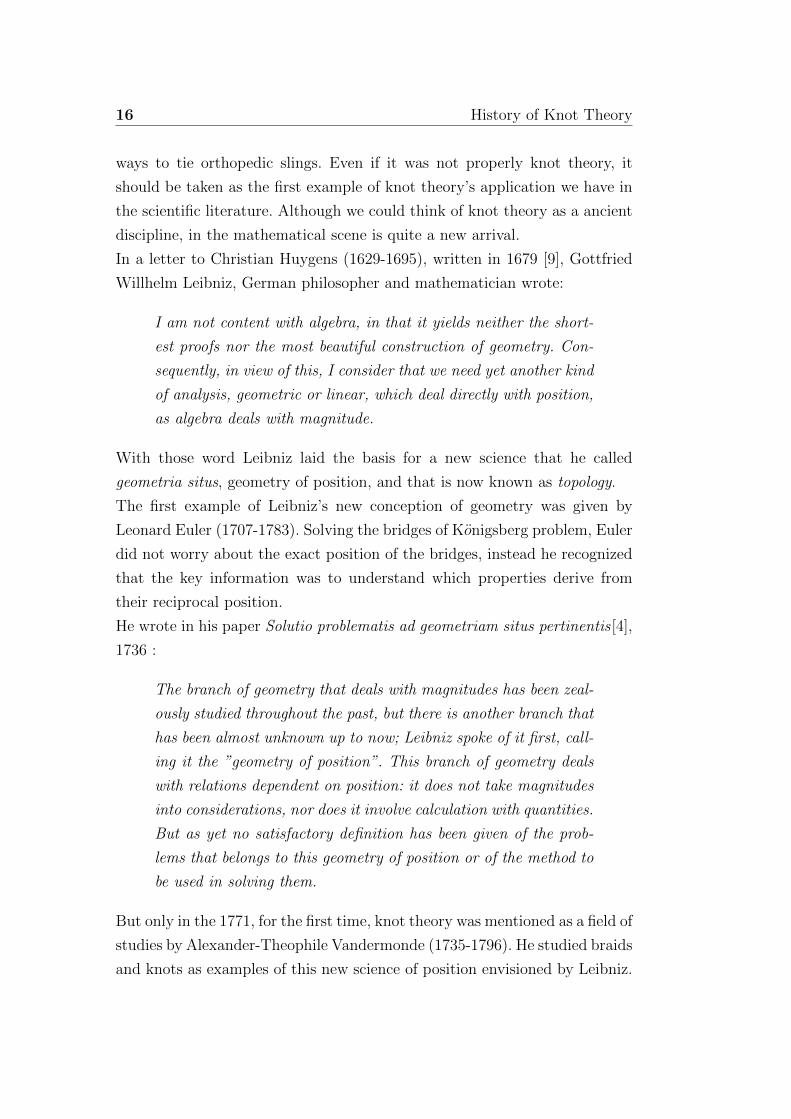
Between 1825 and 1844, he worked on the classification of closed plane curves

with a finite number of self-intersections, which he called Tractfiguren ( we

may think of them as knot projections). His method consisted in giving an

orientation to these curves and then in labeling the crossing with letters.

Therefore he created a sequence, starting from a chosen starting point all

over the tractfiguren. Thus a curve with n crossing would have a sequence of

length 2n. For example, the trefoil knot would be recorded as ABCABC.

Figure 1.2: The Gauss’ labeled scheme of the trefoil ABCABC.

18 History of Knot Theory

Moreover, working in electrodynamics, Gauss discovered the first relevant

result in Knot Theory. His aim was to find a method that could estimate

how much work is done on a magnetic pole moving along a closed curve in

presence of a loop current. During his investigation he discovered what is

called Gauss linking number.

The Gauss linking number is the first invariant discovered1

A main task (that lies) on the border between geometria situs and

geometria magnitudinis is to count the windings of two closed or

infinite lines . . .m number of the windings. This value is shared,

i.e., it remains the same if the lines are interchanged.[13]

The Gauss linking number was reconsidered by many.

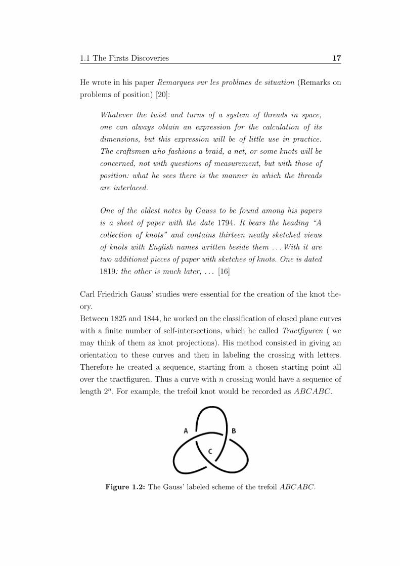
James Clerk Maxwell (1831-1879) showed his interest in this topic and found

two loops that cannot be separated even if their Gauss linking number equals

to 0.

Figure 1.3: In the Hopflink the linking number is 0, but the two loop cannot be

separated.

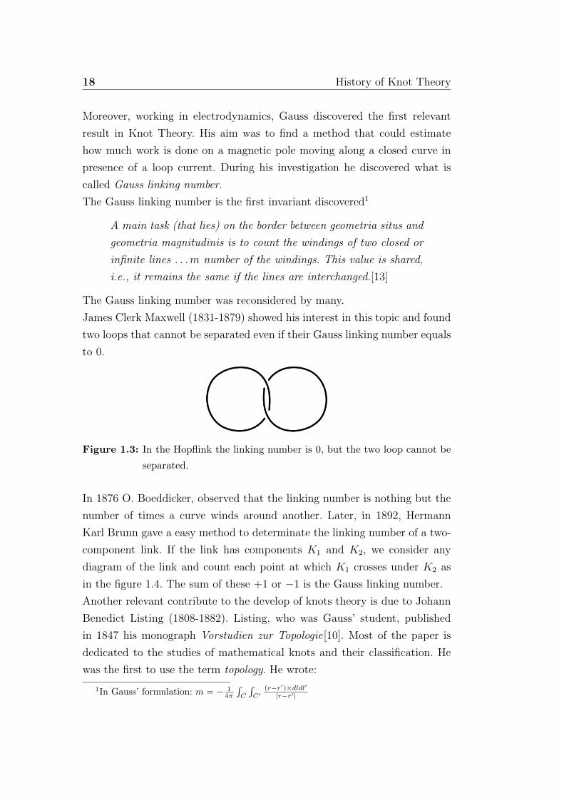
In 1876 O. Boeddicker, observed that the linking number is nothing but the

number of times a curve winds around another. Later, in 1892, Hermann

Karl Brunn gave a easy method to determinate the linking number of a two-

component link. If the link has components K1 and K2, we consider any

diagram of the link and count each point at which K1 crosses under K2 as

in the figure 1.4. The sum of these +1 or −1 is the Gauss linking number.

Another relevant contribute to the develop of knots theory is due to Johann

Benedict Listing (1808-1882). Listing, who was Gauss’ student, published

in 1847 his monograph Vorstudien zur Topologie[10]. Most of the paper is

dedicated to the studies of mathematical knots and their classification. He

was the first to use the term topology. He wrote:

1In Gauss’ formulation: m = − 14π

∫C

∫C′

(r−r′)×dldl′|r−r′|

1.2 Physic’s interest in knot theory 19

Figure 1.4: The linking number.

I hope you let me use the name “Topology for this kind of stud-

ies of spatial images, rather than suggested by Leibniz name “ge-

ometria situs, reminding of notion of “measure” and “measure-

ment”, playing here absolutely subordinate role and confiding with

“geometrie de position” which is established for a different kind

of geometrical studies. Therefore, by Topology we will mean the

study of modal relation and spacial image, or of laws of connected-

ness, mutual disposition and traces of points, lines surface, bodies

and their parts or their unions in space, independently of relations

of measures and quantities.

Listing was interested in developing an algebraic calculus of knot diagrams

so that it could easily be determined when two diagrams represented the

same knot. In particulary, he showed interest in the chirality of a knots, i.e.

the isotopy between knot and its mirror image. He was the first to state that

the right handed trefoil and the left handed trefoil are not isotopic. On the

contrary the figure eight knot also known as the Listing knot is achiral, that

is it’s equivalent to his mirror image. (see 1.5)

2 Physic’s interest in knot theory

During the 1860’s the scientific community was divided in two: the ones that

believed that the matter is composed by atoms (“corpuscular theory”), and

the others, that believe that the matter was behaving as waves. In 1867,

William Thomson, later to be Lord Kelvin (1824-1907), recognized that the

particular shape of a vortex was not as important as the underlying topologi-

cal structure, and felt that an understanding of such vortices would lead to a

complete understanding of matter. Inspired by Helmholtz’s considerations[5],

20 History of Knot Theory

he wrote all his ideas in the essay, “On vortex atoms”[17], in which he assume

that the matter consisted of vortex atoms.

After noticing Helmholtz’s admirable discovery of the law of vor-

tex motion in a perfect liquid, that is, in a fluid perfectly destitute

of viscosity (or fluid friction), the author said that this discov-

ery inevitably suggest that the Helmholtz’s ring are the only true

atoms.

According to Thomson’s idea, atoms have the same shape as a vortex that

is flowing in the ether, a perfect fluid, that can possibly be knotted, but

still maintain its identity. Then atoms are simply knots and a molecule is a

composition of knots.

This seems so absurd now that we have knowledge of atoms and constituents

of matter, but one should think about string theory, our new model in the

infinite small, which does not look more reasonable or realistic from vortex

theory.

With this new theory, the interest for knots theory increased in the scien-

tific society. If the atoms were modeled by knots, then the next problem

was trying to classify them. A first attempt in this direction is due to the

physicist Peter Guthrie Tait (1831-1901). Despite his important role in the

development of Thomsons idea, Tait initially felt that Thomson was wrong.

He felt that vortex motions principal application would be in the theory of

electromagnetism. Anyway, despite Taits initial objection, Thomson contin-

ued thinking about atoms as vortices, sparking the interest of James Clerk

Maxwell. Maxwell had been doing work in electromagnetism for some time.

However, he was also open to the idea that knotted vortices could be the fun-

damental building blocks of matter. So he started a discussions which went

on in letters exchanged with Tait and Thomson about some of his ideas and

discoveries. They were very interested in his ideas. In fact he rediscovered

an integral formula counting the linking number of two closed curves which

Gauss had discovered, but had not published and also gave equations for

knotted curves in a three dimensional space. Moreover, in his letter, he noted

that the trefoil was the simplest knot that was truly knotted that consisted

of a single strand. He went on to recognize a parameter in his equations that

1.2 Physic’s interest in knot theory 21

could determine if the trefoil thus produced was right-handed or left-handed

and claimed (without proof) that there was no way to change a right-handed

trefoil into a left-handed one or vice versa.

Figure 1.5: The left-handed and right-hand trefoil.

Thus in a couple of days, Maxwell had anticipated much of what would

happen in knot theory over the next 80 years. Maxwell’s research was directed

to determinate whether two projections of a knot represented the same knot.

In order to answer his question, he created a labeling scheme for the crossing

points of a knot projection and then showed that every knot diagram must

contain a region bounded by fewer than four arcs, where he defined an arc

to be a segment of the projection from one crossing point to the next. So, he

began to determine all of the possibilities for such regions using this scheme.

In the case of a region bounded by one arc, this was simply a twist as shown

in 1.6, which could easily be undone without changing the knot. For regions

bounded by two arcs, he found two possibilities. Namely, a region created as

a strand passed over another strand at two consecutive points or a region

created as a strand passed over and then under another. (See 1.6.) In the

Figure 1.6: The regions bounded by less than 4 arcs.

first case, the top strand can be moved so that it no longer crosses over the

bottom strand without changing the link type; the second however, could not

be undone. Surprisingly, the situation gets no more complicated with regions

bounded by three arcs, where there are two possible cases as shown in Figure

1.6. Regarding this situation he wrote in [11]

In the first case, any one curve can be moved past the intersection

of the other two without disturbing them. In the second case this

22 History of Knot Theory

cannot be done and the intersection of two curves is a bar to the

motion of the third in that direction.

Although his approach contained no mathematical rigor, it is remarkable to

note that Maxwell had defined the ”Reidemeister moves” which would be

shown to be the fundamental moves in modifying knots only in the 1920s.

In the meantime, Tait gradually changed his mind, and started to tabulate

knots, hoping to create a table of elements to go with Thomson’s atomic

theory. By 1876 he had set out to make a complete table of knots up to

seven crossings. However he understood that the complexity of the knots he

was producing would prevent them from all being stable enough as vortices

to represent atoms, meaning that a tabulation of knots with higher crossing

numbers would be required[14]. Such a tabulation would require more efficient

methods for determining if two knot diagrams were the same, an idea that

would not be realized for over 100 years.

The development of this subject promises absolutely endless work,

but work of a very interesting and useful kind, because it is in-

timately connected with the theory of knots, which (especially as

applied in Sir W. Thomsons Theory of Vortex Atoms) is likely

soon to become an important branch of mathematics.

Taits serious investigation of knots began, as for Gauss and Maxwell, with

the development of a way to symbolically encode the crossings of a knot

projection. Tait developed his own encoding scheme. During his research he

introduced three principles, known as Tait conjectures. In order to simplify

his work he decided to work only with alternating knots, namely those which

have an upper crossing followed by an under crossing. Guided by the evidence

from these alternating diagram, he stated his first conjecture.

Conjecture 1. A reduced alternating knot has minimal crossing number.

Tait’s second conjecture was cryptically stated as If the simplest is + −+−+− then irreducible [2]. The interpretation we have today is the following:

Conjecture 2. An alternating knot diagram without nugatory crossings,

those that separate two nontrivial distinct portions of the knot, cannot be

manipulated to have fewer crossings.

1.2 Physic’s interest in knot theory 23

For example, the trefoil and figure-8 knot cannot be drawn with fewer cross-

ings, as they are both depicted as alternating knots without nugatory cross-

ings. This conjecture was first rigorously proved by Murasugi in [12], only

after the discovery of the Jones polynomial. Tait was not so sure of his third

conjecture, today best known as Tait’s flyping conjecture, which is usually

stated as

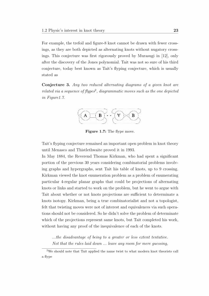
Conjecture 3. Any two reduced alternating diagrams of a given knot are

related via a sequence of flypes2, diagrammatic moves such as the one depicted

in Figure1.7.

Figure 1.7: The flype move.

Tait’s flyping conjecture remained an important open problem in knot theory

until Menasco and Thistlethwaite proved it in 1993.

In May 1884, the Reverend Thomas Kirkman, who had spent a significant

portion of the previous 30 years considering combinatorial problems involv-

ing graphs and hypergraphs, sent Tait his table of knots, up to 9 crossing.

Kirkman viewed the knot enumeration problem as a problem of enumerating

particular 4-regular planar graphs that could be projections of alternating

knots or links and started to work on the problem, but he went to argue with

Tait about whether or not knots projections are sufficient to determinate a

knots isotopy. Kirkman, being a true combinatorialist and not a topologist,

felt that twisting moves were not of interest and equivalences via such opera-

tions should not be considered. So he didn’t solve the problem of determinate

which of the projections represent same knots, but Tait completed his work,

without having any proof of the inequivalence of each of the knots.

...the disadvantage of being to a greater or less extent tentative.

Not that the rules laid down ... leave any room for mere guessing,

2We should note that Tait applied the name twist to what modern knot theorists call

a flype

24 History of Knot Theory

but they are too complex to be always completely kept in view.

Thus we cannot be absolutely certain that by means of such pro-

cesses we have obtained all the essentially different forms which

the definition we employ comprehends.

In 1899 Charles Newton Little classified non alternating knots up to 10 cross-

ing. He took 6 years to complete his work.

Many more scientists continued to tabulate knots for the next years. These

tables were partially extended in M.G. Hasemans doctoral dissertation of

1916. Knots up to 11 crossings were enumerated by John H. Conway before

1969. Knots up to 13 crossings were enumerated by C .H .Dowker and M.

B. Thistlethwaite in 1983. Nowadays, computerization of the problem has

made knot enumeration considerably easier, but the rapid growth in the

number of knots is still astonishing. For example in a July 2003 tabulation

of all prime, alternating knots through 22 crossings performed by S. Rankin,

J. Schermann, and O. Smith have been found 6, 217, 553, 258 knots. The

counting of knots is one part of the history of knot theory, however other are

the disciplines that make knot theory develop.

3 The modern knot theory

Even though Thomson’s vortex atoms were of course abandoned, pure Mathe-

maticians were still interesting in knot theory. Poincare introduced the Fun-

damental group about 1900. The fundamental group was a significant ad-

vance in the study of topology, since it created a way for using the tools

of abstract algebra for studying the field of topology. Shortly after its dis-

covery, it was applied to knot theory. In 1908, Heinrich Tietze (1880-1964)

used the fundamental group of the complement of a knot in R3, called the

knot group, in order to distinguish the unknot from the trefoil knot [18]. The

Austrian mathematician Wilhelm Wirtinger (1865-1945), whose work was

actually motivated by the study of algebraic functions of a single complex

variable, showed in his lecture delivered at a meeting of the German Mathe-

matical Society in 1905 a method for finding a knot group presentation (it is

called now the Wirtinger presentation of a knot group). Later, Max Dehn,

a German mathematician who studied under Hilbert, became interested in

1.3 The modern knot theory 25

the theory of knots as he worked to prove the Poincare conjecture. Of course,

Dehn did not prove the Poincare conjecture, but he did develop another algo-

rithm (distinct from Wirtingers) for constructing the fundamental group of

the complement of a link. Using this, Dehn showed that a knot is nontrivial if

and only if its fundamental group is non-abelian. He went on to show that a

trefoil knot and its mirror image are different. That is, Dehn showed that the

trefoil knot is not achiral. The work of Dehn and his colleagues came to a halt

with the outbreak of World War I, and it would not be until after the war

that any significant work in knot theory resumed. The breakthrough in knot

theory is due to James W. Alexander at Princeton and Kurt Reidemeister in

Vienna. In the 1920s, independently, both of them arrived at the same knot

invariant. Alexander used the homology groups while Reidemeister used the

fundamental groups.

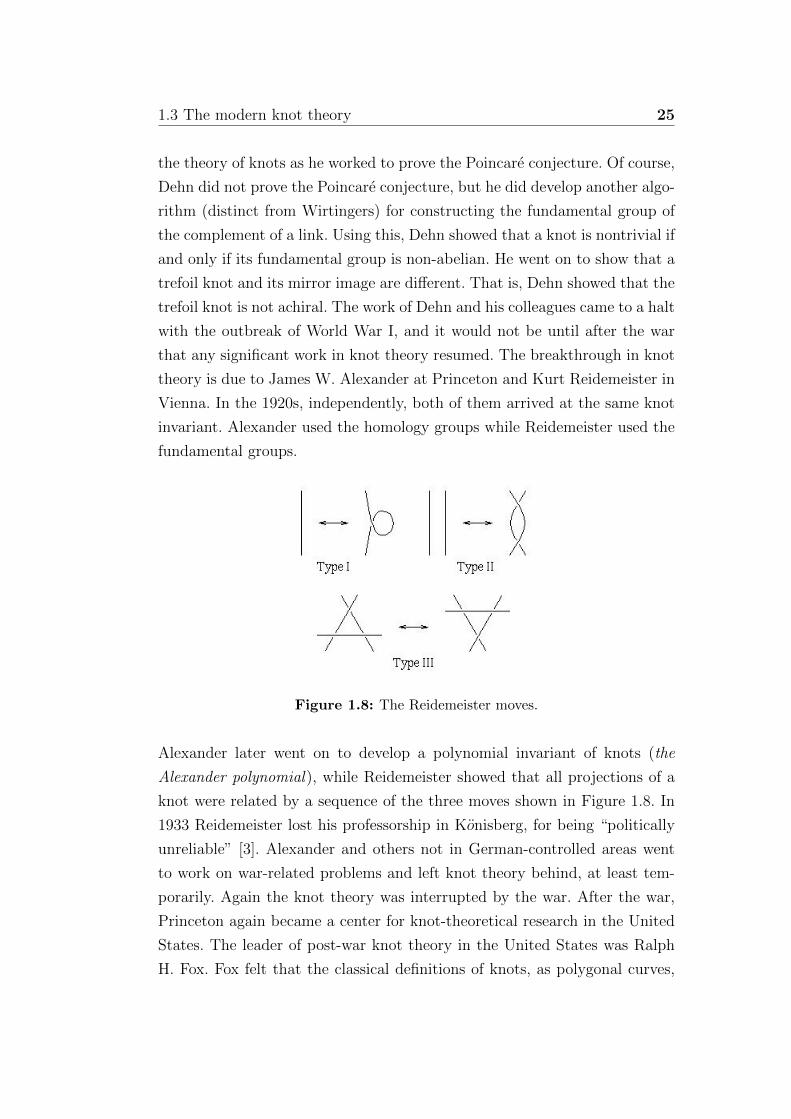
Figure 1.8: The Reidemeister moves.

Alexander later went on to develop a polynomial invariant of knots (the

Alexander polynomial), while Reidemeister showed that all projections of a

knot were related by a sequence of the three moves shown in Figure 1.8. In

1933 Reidemeister lost his professorship in Konisberg, for being “politically

unreliable” [3]. Alexander and others not in German-controlled areas went

to work on war-related problems and left knot theory behind, at least tem-

porarily. Again the knot theory was interrupted by the war. After the war,

Princeton again became a center for knot-theoretical research in the United

States. The leader of post-war knot theory in the United States was Ralph

H. Fox. Fox felt that the classical definitions of knots, as polygonal curves,

26 History of Knot Theory

caused knot theory to be too disconnected from the rest of topology. He re-

defined a knot with topologically-defined set of curves and instead of R3 he

propose to insert a knot in other compact 3-manifolds. Fox’s work led to a

number of new geometric knot invariants. In the 1970s, J.H. Conway was

doing more than simply tabulating knots as discussed in the previous sec-

tion. He devised a new way to calculate the Alexander polynomial using an

algorithm on knot diagrams. In fact, his work actually led to a refinement of

the Alexander polynomial that is often called the Conway polynomial. The

main breakthrough in knot theory occurred in 1984 when Vaughan Jones

developed a new polynomial invariant of knots (the Jones polynomial) as he

conducted research on von Neumann algebras. The Jones polynomial was a

significant improvement over the earlier polynomial invariants as it was able

to distinguish many knots from their mirror images. Four months after the

discovery of the Jones polynomial, an invariant called the HOMFLY poly-

nomial was discovered. Its name derived from the name of the scientists who

discovered it, Jim Hoste, Adrian Ocneanu, Kenneth Millett, Peter J. Freyd,

W. B. R. Lickorish, and David Nelson Yetter. This polynomial is a gener-

alization of the Jones polynomial, and in most of the cases it detects the

chirality of knots. In August 1985 mathematician Louis H. Kauffman (1945,-

) employing techniques used in the study of statistical physics, discovered

another approach to the Jones polynomial, the Kauffman bracket. This new

polynomial produced an alternative method for computing the Jones poly-

nomial.

So far, we have seen how knot theory as been developed during the his-

tory, and how new invariants have been discovered according to the different

mathematical theory, used at that precise time. In the next chapter we will

introduce knot theory with a formal approach. We will study different in-

variants, starting from the simplest ones and introduce their mathematical

proprieties.

Chapter 2

Knot invariants

O time! thou must untangle this, not I; It is

too hard a knot for me to untie!

William Shakespeare, Twelfth Night, Act II,

Scene 2

1 Basic concepts

The intuitive notion of a knot is that of a knotted loop of rope. This notion

leads naturally to the definition of a knot as a continuous simple closed curve

in R. Such a curve consists of a continuous function f : [0, 1] → R3 with

f(0) = f(1) and with f(x) = f(y) implying one of three possibilities:x = y;

x = 0 and y = 1; x = 1 and y = 0. Unfortunately this definition admits

pathological or so called wild knots into our studies. The solution is either to

introduce the concept of differentiability or to use polygonal curves instead of

differentiable ones in the definition. The simplest definitions in knot theory

are based on the following approach.

Definition 2.1. A knot is a closed curve in R3 that does not intersect itself.

Projections of a knot on some plane allow the representation of a knot as

a knot diagram. Certain knot projections are better than others as in some

projections too much information is lost.

Definition 2.2. A knot projection is called a regular projection if no three

points on the knot project to the same point, and no two edges of the knot

28 Knot invariants

are mapped onto one another.

Suppose to have two projections of the same knot. If we made a knot out of

a string that modeled the first of the two projections, then we should be able

to rearrange the string to resemble the second projection. This rearranging

of the string, that is, the movement of the string through three-dimensional

space without letting it pass through itself, an ambient isotopy.

Definition 2.3. An planar isotopy is a deformation of a knot projection

within the plane that keeps every crossing intact.

A knot diagram is the regular projection of a knot to the plane with broken

lines indicating where one part of the knot undercrosses the other part. In-

formally, an orientation of a knot can be thought of as a direction of travel

around the knot.

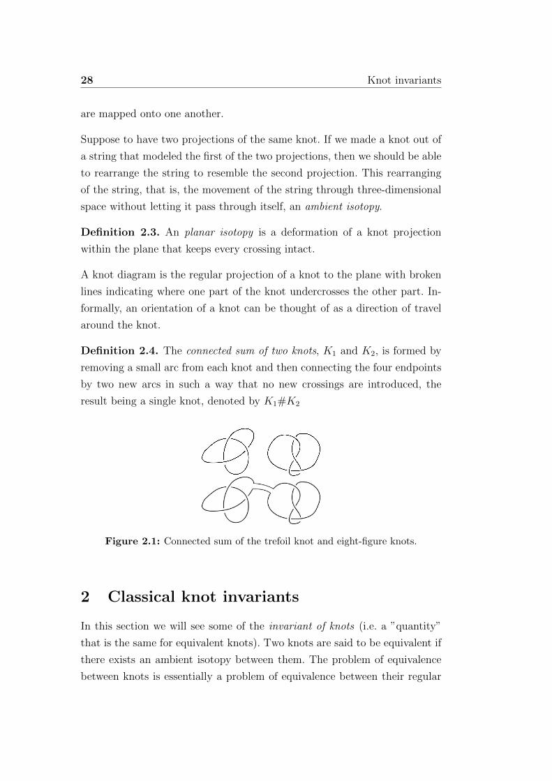
Definition 2.4. The connected sum of two knots, K1 and K2, is formed by

removing a small arc from each knot and then connecting the four endpoints

by two new arcs in such a way that no new crossings are introduced, the

result being a single knot, denoted by K1#K2

Figure 2.1: Connected sum of the trefoil knot and eight-figure knots.

2 Classical knot invariants

In this section we will see some of the invariant of knots (i.e. a ”quantity”

that is the same for equivalent knots). Two knots are said to be equivalent if

there exists an ambient isotopy between them. The problem of equivalence

between knots is essentially a problem of equivalence between their regular

2.2.1 The Reidemeister moves 29

projections. In fact the first invariant we will show consist of three moves

that Reidemeister discovered, that can deform a knot projection into another

one, keeping the knots represented by those two projections, equivalent. We

will also see other invariants that are quite elementary, that follow from the

observation of the knot projections, such as the number of crossing points,

the bridge number, the linking number and the tricolorability.

2.1 The Reidemeister moves

In 1926, the German mathematician Kurt Reidemeister (1893-1971) proved

that if we have two diagrams of the same knot, we can get from the one

diagram to the other by a series of Reidemeister moves and planar isotopies.

Definition 2.5. A Reidemeister move is one of three following ways to

change a projection of the knot.

• First Reidemeister move: allows us to put in or take out a twist in the

knot, as in fig.2.2;

• Second Reidemeister move: allows us to either add two crossings or

remove two crossings, as in fig.2.2;

• Third Reidemeister move: allows us to slide a strand of the knot from

one side of a crossing to the other side of the crossing, as in fig.2.2 .

Figure 2.2: The Reidemeister moves.

Reidemeister proved the following theorem [8]:

30 Knot invariants

Theorem 2.1. Two knots K and K ′ with diagram D and D′ are equivalent

if and only D = D0, D1, . . . , Dn = ”D′ of intermediate diagrams such that

each differs from its predecessor by one of the three Reidemeisteir moves.

In the light of Reidemeister theorem it may seems that the problem of deter-

mining whether two projections represent the same knot is easy: it is enough

to check whether or not there is a sequence of Reidemeister moves taking

from one projection to the other. But taking from one projection to the

other could require an infinite number or Reidemeister moves. For instance,

the trefoil knot is not achiral, but there is no proof in term of Reidemeister

moves. Even if we could prove that we cannot get from the standard projec-

tion of the trefoil knot to its mirror image in 10000006 Reidemeister moves,

maybe we could do it with 10000007 moves.

2.2 The minimum number of crossing points

A diagram D of a knot K has at most a finite number of crossing points.

However, this number c(D) is not a knot invariant. For example, the trivial

knot has two regular projections D and D′, which have a different number

of crossing points.

Figure 2.3: Two diagrams of the unknotted with different crossing number.

Consider all the diagrams of K and let c(K) be the minimum number of

crossing points of all the diagrams. This c(K) is a knot invariant.

Theorem 2.2.

c(K) = minDc(D)

is a knot invariant, where D is the set of all the diagrams, D, of K.

Proof. Suppose that D0 is the minimum diagram of K. Let K ′ be a knot

that is equivalent to K, and suppose that D′0 is its minimum diagram. Since

2.2.3 The bridge number 31

D′0 is a diagram also for K (K and K ′ are equivalent), from the definition

we have that c(D0) ≤ c(D′0). However, since D0 is a diagram of K ′, it again

follows from the definition that c(D′0) ≤ c(D0). Hence, combining the two

inequalities, we obtain c(D0) = c(D′0), i.e., c(D0) is the minimum number

of crossing points for all knots equivalent to K. Consequently, it is a knot

invariant.

2.3 The bridge number

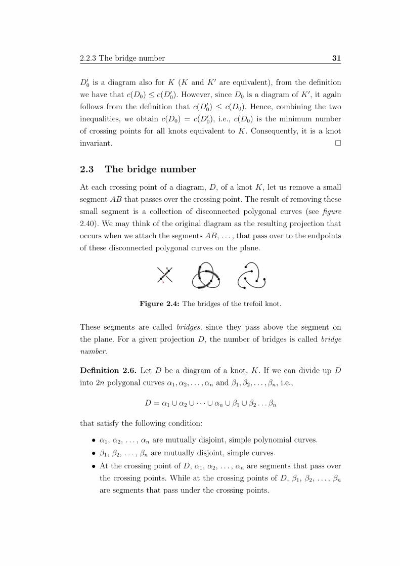
At each crossing point of a diagram, D, of a knot K, let us remove a small

segment AB that passes over the crossing point. The result of removing these

small segment is a collection of disconnected polygonal curves (see figure

2.40). We may think of the original diagram as the resulting projection that

occurs when we attach the segments AB, . . . , that pass over to the endpoints

of these disconnected polygonal curves on the plane.

Figure 2.4: The bridges of the trefoil knot.

These segments are called bridges, since they pass above the segment on

the plane. For a given projection D, the number of bridges is called bridge

number.

Definition 2.6. Let D be a diagram of a knot, K. If we can divide up D

into 2n polygonal curves α1, α2, . . . , αn and β1, β2, . . . , βn, i.e.,

D = α1 ∪ α2 ∪ · · · ∪ αn ∪ β1 ∪ β2 . . . βn

that satisfy the following condition:

• α1, α2, . . . , αn are mutually disjoint, simple polynomial curves.

• β1, β2, . . . , βn are mutually disjoint, simple curves.

• At the crossing point of D, α1, α2, . . . , αn are segments that pass over

the crossing points. While at the crossing points of D, β1, β2, . . . , βn

are segments that pass under the crossing points.

32 Knot invariants

then the bridge number of D, br(D), is said to be at most n.

If br(D) ≤ n but br(D) � n− 1, we define br(D) = n.

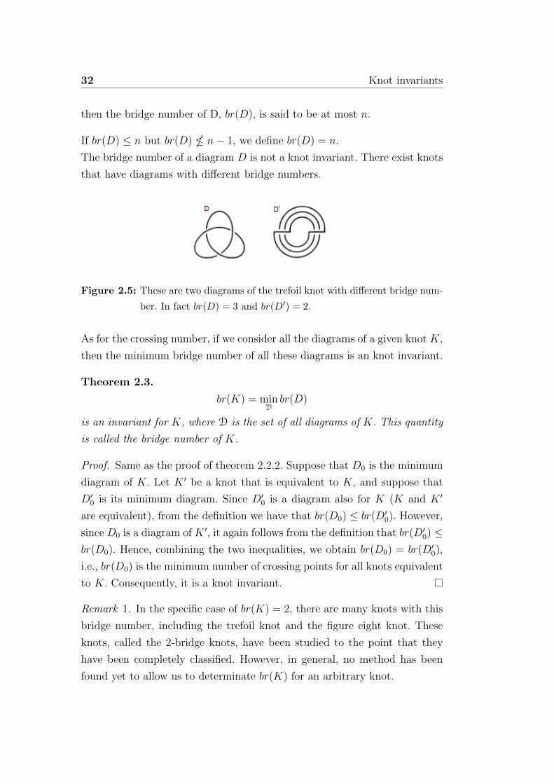
The bridge number of a diagram D is not a knot invariant. There exist knots

that have diagrams with different bridge numbers.

Figure 2.5: These are two diagrams of the trefoil knot with different bridge num-

ber. In fact br(D) = 3 and br(D′) = 2.

As for the crossing number, if we consider all the diagrams of a given knot K,

then the minimum bridge number of all these diagrams is an knot invariant.

Theorem 2.3.

br(K) = minDbr(D)

is an invariant for K, where D is the set of all diagrams of K. This quantity

is called the bridge number of K.

Proof. Same as the proof of theorem 2.2.2. Suppose that D0 is the minimum

diagram of K. Let K ′ be a knot that is equivalent to K, and suppose that

D′0 is its minimum diagram. Since D′0 is a diagram also for K (K and K ′

are equivalent), from the definition we have that br(D0) ≤ br(D′0). However,

since D0 is a diagram of K ′, it again follows from the definition that br(D′0) ≤br(D0). Hence, combining the two inequalities, we obtain br(D0) = br(D′0),

i.e., br(D0) is the minimum number of crossing points for all knots equivalent

to K. Consequently, it is a knot invariant.

Remark 1. In the specific case of br(K) = 2, there are many knots with this

bridge number, including the trefoil knot and the figure eight knot. These

knots, called the 2-bridge knots, have been studied to the point that they

have been completely classified. However, in general, no method has been

found yet to allow us to determinate br(K) for an arbitrary knot.

2.2.4 The linking number 33

2.4 The linking number

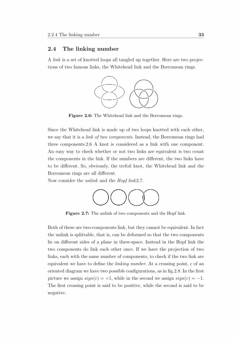
A link is a set of knotted loops all tangled up together. Here are two projec-

tions of two famous links, the Whitehead link and the Borromean rings.

Figure 2.6: The Whitehead link and the Borromean rings.

Since the Whitehead link is made up of two loops knotted with each other,

we say that it is a link of two components. Instead, the Borromean rings had

three components.2.6 A knot is considered as a link with one component.

An easy way to check whether or not two links are equivalent is two count

the components in the link. If the numbers are different, the two links have

to be different. So, obviously, the trefoil knot, the Whitehead link and the

Borromean rings are all different.

Now consider the unlink and the Hopf link2.7.

Figure 2.7: The unlink of two components and the Hopf link.

Both of these are two-components link, but they cannot be equivalent. In fact

the unlink is splittable, that is, can be deformed so that the two components

lie on different sides of a plane in three-space. Instead in the Hopf link the

two components do link each other once. If we have the projection of two

links, each with the same number of components, to check if the two link are

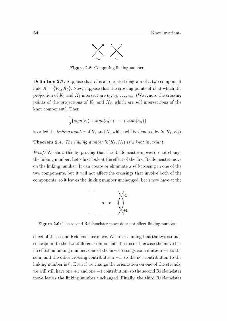
equivalent we have to define the linking number. At a crossing point, c of an

oriented diagram we have two possible configurations, as in fig.2.8. In the first

picture we assign sign(c) = +1, while in the second we assign sign(c) = −1.

The first crossing point is said to be positive, while the second is said to be

negative.

34 Knot invariants

Figure 2.8: Computing linking number.

Definition 2.7. Suppose that D is an oriented diagram of a two component

link, K = {K1, K2}. Now, suppose that the crossing points of D at which the

projection of K1 and K2 intersect are c1, c2, . . . , cm. (We ignore the crossing

points of the projections of K1 and K2, which are self intersections of the

knot component). Then

1

2{sign(c1) + sign(c2) + · · ·+ sign(cm)}

is called the linking number ofK1 andK2 which will be denoted by lk(K1, K2).

Theorem 2.4. The linking number lk(K1, K2) is a knot invariant.

Proof. We show this by proving that the Reidemeister moves do not change

the linking number. Let’s first look at the effect of the first Reidemeister move

on the linking number. It can create or eliminate a self-crossing in one of the

two components, but it will not affect the crossings that involve both of the

components, so it leaves the linking number unchanged. Let’s now have at the

Figure 2.9: The second Reidemeister move does not effect linking number.

effect of the second Reidemeister move. We are assuming that the two strands

correspond to the two different components, because otherwise the move has

no effect on linking number. One of the new crossings contributes a +1 to the

sum, and the other crossing contributes a −1, so the net contribution to the

linking number is 0. Even if we change the orientation on one of the strands,

we will still have one +1 and one −1 contribution, so the second Reidemeister

move leaves the linking number unchanged. Finally, the third Reidemeister

2.2.5 The tricolorability 35

move doesn’t effect linking number either. Once orientation is chosen for each

of the three strands and +1 and −1 are assigned to each of the crossing, it is

clear that sliding the strand over during the third Reidemeister move doesn’t

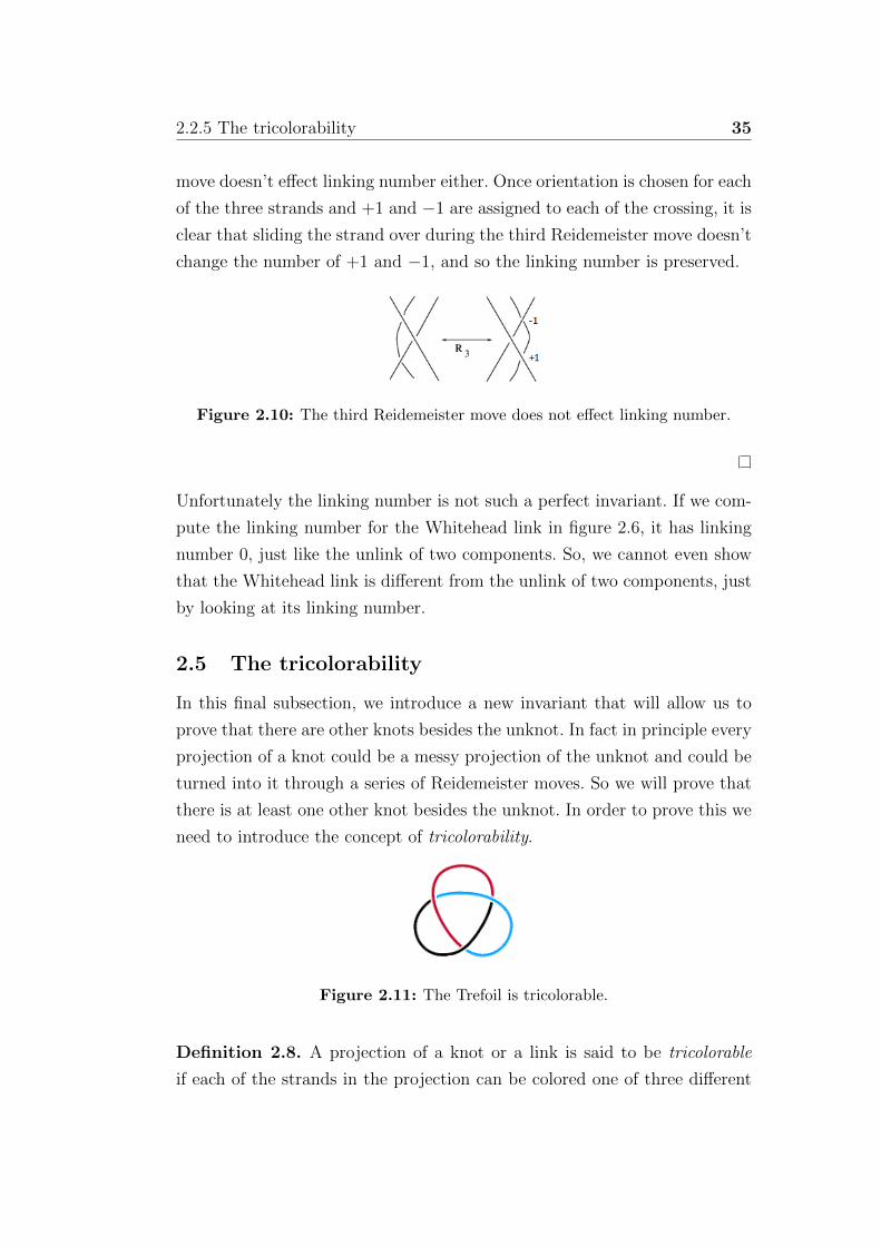
change the number of +1 and −1, and so the linking number is preserved.

Figure 2.10: The third Reidemeister move does not effect linking number.

Unfortunately the linking number is not such a perfect invariant. If we com-

pute the linking number for the Whitehead link in figure 2.6, it has linking

number 0, just like the unlink of two components. So, we cannot even show

that the Whitehead link is different from the unlink of two components, just

by looking at its linking number.

2.5 The tricolorability

In this final subsection, we introduce a new invariant that will allow us to

prove that there are other knots besides the unknot. In fact in principle every

projection of a knot could be a messy projection of the unknot and could be

turned into it through a series of Reidemeister moves. So we will prove that

there is at least one other knot besides the unknot. In order to prove this we

need to introduce the concept of tricolorability.

Figure 2.11: The Trefoil is tricolorable.

Definition 2.8. A projection of a knot or a link is said to be tricolorable

if each of the strands in the projection can be colored one of three different

36 Knot invariants

chosen colors, so that at each crossing, either three different colors come

together or all the same color comes together. In order that a projection be

tricolorable, is also required that at least two colors are used.

Example 1. The unknot is not tricolorable. We certainly cannot use at least

two colors on it.

Theorem 2.5. The tricolorability of a knot is a knot invariant.

Proof. We have to show that the Reidemeister moves will preserve the tri-

colorability. If we do a first Reidemeister move and introduce a crossing, we

can just leave all the strands involved the same color, and the new crossing

will satisfy the requirements for tricolorability. Similarly, removing a crossing

with the first Reidemeister move preserves tricolorability.

Figure 2.12: The first Reidemeister move preserves tricolorability.

If we do a second Reidemeister move and introduce two crossings and the

two original strands are different colors, we can change the color of the new

strand to the third color, and the resulting knot projection is tricolorable. If

the two original strands are the same colors we can leave the new strand and

the new crossings all the same color.

Figure 2.13: The second Reidemeister move preserves tricolorability.

Similarly, using a second Reidemeister move to reduce the number of crossings

by two will also preserve tricolorability. Either all of the strands that appear

in the projection for the Reidemeister move are the same color, in which case

2.2.5 The tricolorability 37

we can color the strands that result from the Reidemeister move that same

color, or three distinct colors come together at each of the two crossings,

in which case we can color the two resulting strands in two different colors.

In both cases, since the original projection was colored with at least two

distinct colors, the resulting projection will also be colored with at least two

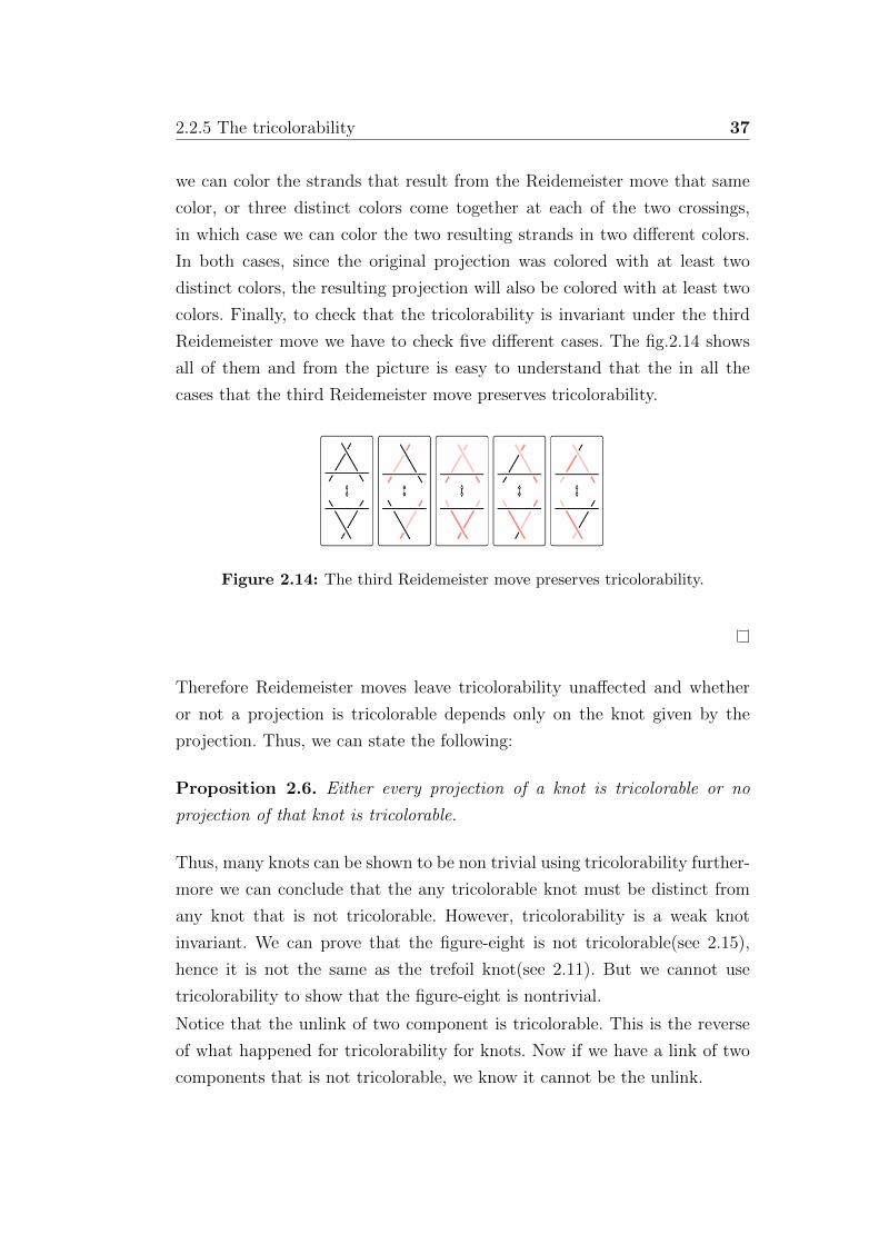
colors. Finally, to check that the tricolorability is invariant under the third

Reidemeister move we have to check five different cases. The fig.2.14 shows

all of them and from the picture is easy to understand that the in all the

cases that the third Reidemeister move preserves tricolorability.

Figure 2.14: The third Reidemeister move preserves tricolorability.

Therefore Reidemeister moves leave tricolorability unaffected and whether

or not a projection is tricolorable depends only on the knot given by the

projection. Thus, we can state the following:

Proposition 2.6. Either every projection of a knot is tricolorable or no

projection of that knot is tricolorable.

Thus, many knots can be shown to be non trivial using tricolorability further-

more we can conclude that the any tricolorable knot must be distinct from

any knot that is not tricolorable. However, tricolorability is a weak knot

invariant. We can prove that the figure-eight is not tricolorable(see 2.15),

hence it is not the same as the trefoil knot(see 2.11). But we cannot use

tricolorability to show that the figure-eight is nontrivial.

Notice that the unlink of two component is tricolorable. This is the reverse

of what happened for tricolorability for knots. Now if we have a link of two

components that is not tricolorable, we know it cannot be the unlink.

38 Knot invariants

Figure 2.15: The figure-eight knot is not tricolorable.

3 Seifert matrix and its invariants

In this section we will introduce the concept of seifert surface, and show how

this concept is related to the knots. Given any knot, in fact, there is a col-

lection of orientable surfaces whose boundary is the knot. We introduce this

new concepts, in order to obtain an important knot invariant, the Alexander

polynomial.

3.1 Seifert matrix

In order to define a Seifert surface, we will start with the following theorem:

Theorem 3.1. Given an arbitrary knot K, then there exists in R3 an ori-

entable, connected surface, F , that has as its boundary K.

The Seifert algorithm will give as a proof of the theorem. We briefly sketch

it.

Suppose that K is an oriented knot and D is a regular diagram for K. Now,

we have to decompose D into several simple closed curves. First we need to

draw a small circle with one of the crossing points of D as its center. This

circle intersects D at four points, say, a, b, c, and d. Let us splice this crossing

points and connect a and d, and b and c as in fig.2.16.

Figure 2.16: Splicing of a knot.

2.3.1 Seifert matrix 39

This operation is called the splicing of a knot K at a crossing point of D.

Performing the splicing operation at every crossing of D we shall remove all

the crossing points from D. The result is that D becomes decomposed into

several simple closed curves. These curves are called Seifert curves. D itself

has been transformed into a diagram of a link on the plane without crossing,

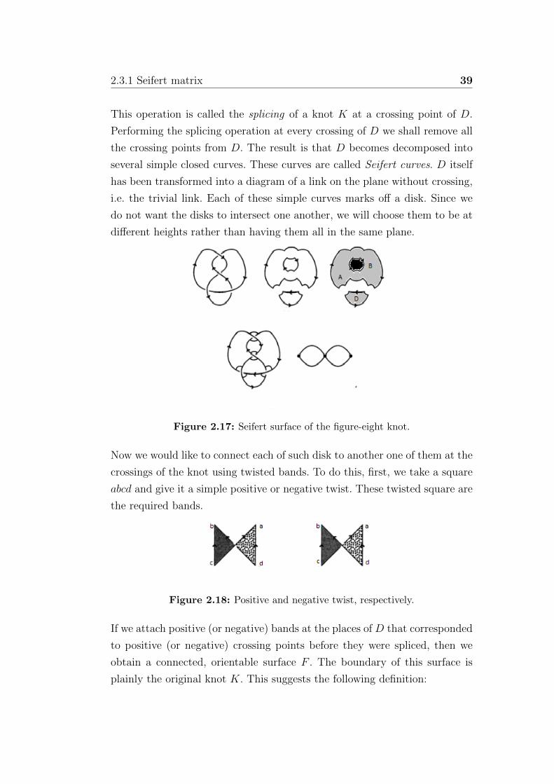
i.e. the trivial link. Each of these simple curves marks off a disk. Since we

do not want the disks to intersect one another, we will choose them to be at

different heights rather than having them all in the same plane.

Figure 2.17: Seifert surface of the figure-eight knot.

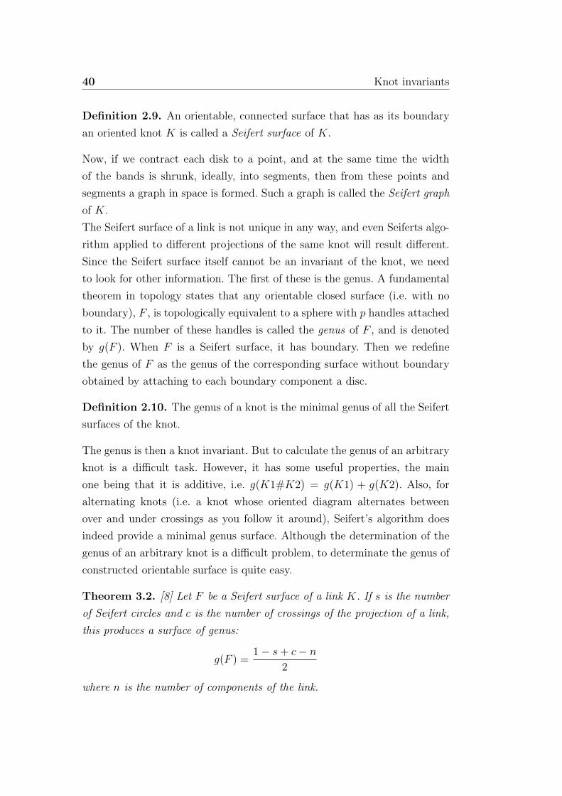
Now we would like to connect each of such disk to another one of them at the

crossings of the knot using twisted bands. To do this, first, we take a square

abcd and give it a simple positive or negative twist. These twisted square are

the required bands.

Figure 2.18: Positive and negative twist, respectively.

If we attach positive (or negative) bands at the places of D that corresponded

to positive (or negative) crossing points before they were spliced, then we

obtain a connected, orientable surface F . The boundary of this surface is

plainly the original knot K. This suggests the following definition:

40 Knot invariants

Definition 2.9. An orientable, connected surface that has as its boundary

an oriented knot K is called a Seifert surface of K.

Now, if we contract each disk to a point, and at the same time the width

of the bands is shrunk, ideally, into segments, then from these points and

segments a graph in space is formed. Such a graph is called the Seifert graph

of K.

The Seifert surface of a link is not unique in any way, and even Seiferts algo-

rithm applied to different projections of the same knot will result different.

Since the Seifert surface itself cannot be an invariant of the knot, we need

to look for other information. The first of these is the genus. A fundamental

theorem in topology states that any orientable closed surface (i.e. with no

boundary), F , is topologically equivalent to a sphere with p handles attached

to it. The number of these handles is called the genus of F , and is denoted

by g(F ). When F is a Seifert surface, it has boundary. Then we redefine

the genus of F as the genus of the corresponding surface without boundary

obtained by attaching to each boundary component a disc.

Definition 2.10. The genus of a knot is the minimal genus of all the Seifert

surfaces of the knot.

The genus is then a knot invariant. But to calculate the genus of an arbitrary

knot is a difficult task. However, it has some useful properties, the main

one being that it is additive, i.e. g(K1#K2) = g(K1) + g(K2). Also, for

alternating knots (i.e. a knot whose oriented diagram alternates between

over and under crossings as you follow it around), Seifert’s algorithm does

indeed provide a minimal genus surface. Although the determination of the

genus of an arbitrary knot is a difficult problem, to determinate the genus of

constructed orientable surface is quite easy.

Theorem 3.2. [8] Let F be a Seifert surface of a link K. If s is the number

of Seifert circles and c is the number of crossings of the projection of a link,

this produces a surface of genus:

g(F ) =1− s+ c− n

2

where n is the number of components of the link.

2.3.1 Seifert matrix 41

Proposition 3.3. [8] If the genus of the Seifert surface, F , of a knot (or

link) is g(F ), then on F there are 2g(F ) + n− 1(= m) closed curves α1, α2,

. . . , αm, where n is the number of components of the link.

These 2g(F ) + n− 1(= m) closed curves will indicate certain characteristics

of the knot K that is the boundary of the surface F . Individually, however,

these closed curves are of little interest, but as a collection they will provide

us with a knot invariant.

Since Seifert surfaces of a given knot, K, are orientable by construction,

inheriting the orientation from the knot, we may think of Seifert surface as

having a positive and negative side. In order to make these side more distinct,

we could make the surface thicker by some ε, where ε > 0 and sufficient small

to not disturb the topology of the surface. Then F × 0 is the negative side

of F , while F × ε is the positive side. Now, consider any closed curve, α on

F . Let α∗ be the curve α which lies on the positive side of F , i.e. α∗ is the

closed curve lying on F × ε.Then we can define the Seifert matrix.

Definition 2.11. Let F be a Seifert surface for a knot with m closed curves

α1,α2, . . . , αm where m is defined above. Then the Seifert matrix is an m×mmatrix,

M = [lk(αi, α∗j )]i,j=1,2,...,m

In general, the linking number lk(αi, α∗j ) and lk(αj, α

∗i ) are not equal, so the

matrix is not a symmetric matrix. In the case when g(F ) = 0, the Seifert

matrix of K is defined to be the empty matrix (K is the trivial knot).

To better understand these concepts, let us consider the figure-eight knot.

In the figure 2.17 we can see the figure-eight knot, its Seifert surface and

the subsequent Seifert graph. Removing the edges from the Seifert graph we

found the spanning tree, that is just three vertices in a line. Adding in the

removed edges one at a time gives us two cycles, one between the top two

vertices, and one between the bottom two vertices.

These correspond to a closed curve, a, between the top and main levels of the

Seifert surface, and a closed curve, b between the base levels of the Seifert

surface respectively. The closed curves are raised slightly above the surface

to better illustrate their path through the crossings. In order to compute the

42 Knot invariants

Figure 2.19: How two find two closed curves in the Seifert surface of the figure-

eight knot.

Seifert matrix for the figure-eight knot we need to find how these two closed

curves link with themselves and each other.

Figure 2.20: The Seifert surface with two closed curves and how these link with

themselves and each other.

From the above four projections, it follows that

lk(a, a∗) = −1, lk(a, b∗) = 1, lk(b, a∗) = 0, lk(b, b∗) = 1

Therefore, the Seifert matrix for the figure-eight knot is

M =

[−1 1

0 1

]In order to obtain an invariant of a knot from a Seifert matrix, we need to

examine the relationship between the Seifert matrices of the same knot. We

need to introduce the concept of the S-equivalence of two square matrices.

Theorem 3.4. Two Seifert matrices, M1 and M2, obtained from two equiv-

alent knots can be changed from one to the other by applying, a finite number

of times, the following two operation, Λ1 and Λ2, and their inverses:

Λ1 : M1 → PM1PT ,

2.3.1 Seifert matrix 43

where P is an invertible integer matrix, with detP = ±1 (detP is just the

usual determinant of P ), and P T denotes the transpose matrix of P .

Λ2 : M1 →M2 =

∗ 0

M1 . . . . . .

∗ 0

0 . . . 0 0 1

0 . . . 0 0 0

or

0 0

M1 . . . . . .

0 0

∗ . . . ∗ 0 0

0 . . . 0 1 0

where * denotes an arbitrary integer.

The operation Λ1 either interchanges two rows, say ith and jth rows, and then

interchanges the ith and jth columns; or it adds k times the ith row to the jth

row, and then adds k times the ith column to the jth column. This operation

is called an elementary symmetric matrix operation. The operation Λ2, on

the other hand, is a matrix operation that is particular to knot theory. This

operation has been defined so that it corresponds to the change in the genus

of the Seifert surface due to a Reidemeister move, i.e. it makes the Seifert

matrix either smaller or larger.

Definition 2.12. Two square matrices M , M ′ obtained one from the other

by applying the operations Λ1, Λ2 and the inverse Λ−12 a finite number of

times, are said to be S-equivalent, and are denoted by MS∼M ′

It follows, from the above theorem, that two Seifert matrices obtained from

the two equivalent knots are S-equivalent.

We shall conclude by proving two properties of Seifert matrices. We denote

by MK the Seifert matrix of a knot of K.

Proposition 3.5. Suppose that K is an oriented knot and −K is the knot

with the reverse orientation to K. Then M−KS∼ MT

K, where MTK is the

transpose matrix of MK.

Proof. If we suppose that D is a diagram of K, we may take as a diagram

D′ for −K, the diagram D with all the orientations reversed. Therefore, the

orientations of the subsequent Seifert surface are completely opposite. Hence,

the under and over relations for ai and a∗j are completely reversed. The Seifert

44 Knot invariants

matrix obtained from D′ is therefore the transpose of that from D. It follows

from theorem that M−KS∼MT

K .

Proposition 3.6. Suppose that K∗ is the mirror image of a knot K, then

MK∗S∼ −MT

K.

Proof. We can obtain a diagram D∗ of K∗ from K by changing the under

and over crossing segment at each of the crossing points. Therefore, since the

under and over relations for the closed curves that follow from D and D∗ are

completely reversed, MK∗S∼ −MT

K .

3.2 The Alexander polynomial

In this section we introduce the Alexander polynomial.

To compute this polynomial let us consider a Seifert matrix M , its transpose

and the polynomial det(M − tMT ) with indeterminate t. Now, we examine

how this polynomial changes when we apply Λ1 and Λ±12 . Firstly, since detP =

detP T = ±1,

det(Λ1(M − tMT )) = det[P (M − tMT )P T ] = det(M − tMT ).

Therefore, it is not affected by the operation Λ1. However, if we apply Λ2,

det(Λ2(M − tMT )) = det

b1 0

M − tMT . . . . . .

bm 0

−b1t . . . −bmt 0 1

0 . . . 0 −t 0

= det

b1 0

M − tMT . . . . . .

bm 0

0 . . . 0 0 1

0 . . . 0 −t 0

= tdet(M − tMT ).

Similarly, we can obtain det(Λ−12 (M2 − tMT2 )) = t−1det(M1 − tMT

1 ).

2.3.2 The Alexander polynomial 45

Theorem 3.7. Suppose that M1 and M2 are the Seifert matrices for a knot

K. Further, if r and s are, respectively, the orders of M1 and M2, then the

following equality holds:

t−r2det(M1 − tMT

1 ) = t−s2det(M2 − tMT

2 ). (2.1)

Therefore, if M is a Seifert matrix of K and its order is k, then

t−k2 det(M − tMT )

is an invariant of K. This invariant is known as the Alexander polynomial

normalized of K and its denoted by ∆K(t). Note that k = 2g(F ) + n − 1,

where F is the Seifert surface, g(F ) is the genus of the surface and n is the

number of components of the link. Sometimes it is preferable to work with

such an interpretation of ∆K(t), like:

∆(K)(t) = tk2 det(M − tMT ). (2.2)

Let us see the Alexander polynomial in some relevant examples.

Example 2. If K is a trivial knot, then ∆K(t) = 1.

Example 3. Let K be the figure-eight knot. As we found above, the Seifert

matrix, M , is:

M =

[−1 1

0 1

]Therefore,

∆K(t) = t−1(M − tMT ) = t−1det

[t− 1 1

−t 1− t

]= −t+ 3− t−1

Example 4. Let us consider the trefoil knot. Let us begin with its knot di-

agram, from which we can construct the Seifert circles and then the Seifert

surface.

We find the closed curves as we did above for the figure-eight knot.

In the following figure, the pairs of curves are display.

We can compute now the linking numbers for the Seifert matrix.

Thus we obtain:

M =

[−1 −1

0 −1

]

46 Knot invariants

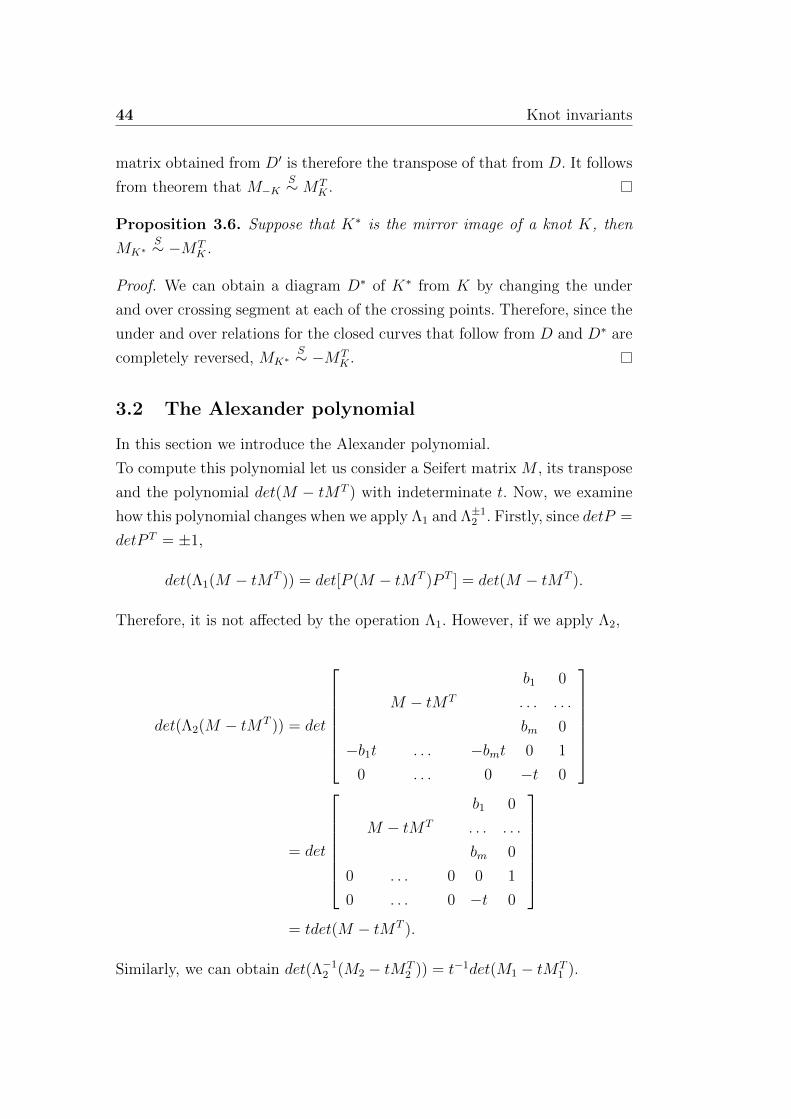
Figure 2.21: The Seifert surface of the trefoil knot.

Figure 2.22: The process of obtaining the closed curves from the Seifert graph

of the trefoil knot.

We can finally compute the Alexander polynomial of the trefoil knot:

∆K(t) = t−1(M − tMT ) = t−1det

[t− 1 −1

t t− 1

]= t− 1 + t−1. (2.3)

3.3 The Alexander-Conway polynomial

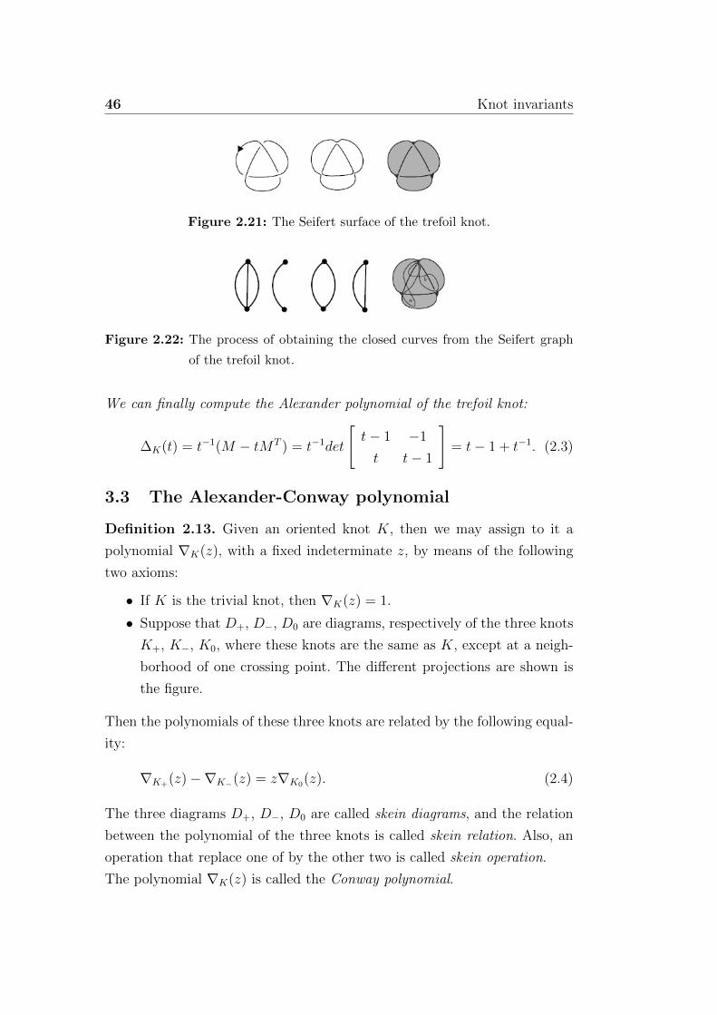
Definition 2.13. Given an oriented knot K, then we may assign to it a

polynomial ∇K(z), with a fixed indeterminate z, by means of the following

two axioms:

• If K is the trivial knot, then ∇K(z) = 1.

• Suppose that D+, D−, D0 are diagrams, respectively of the three knots

K+, K−, K0, where these knots are the same as K, except at a neigh-

borhood of one crossing point. The different projections are shown is

the figure.

Then the polynomials of these three knots are related by the following equal-

ity:

∇K+(z)−∇K−(z) = z∇K0(z). (2.4)

The three diagrams D+, D−, D0 are called skein diagrams, and the relation

between the polynomial of the three knots is called skein relation. Also, an

operation that replace one of by the other two is called skein operation.

The polynomial ∇K(z) is called the Conway polynomial.

2.3.3 The Alexander-Conway polynomial 47

Figure 2.23: How these closed curves link with themselves and each other.

Figure 2.24: Skein diagrams.

Theorem 3.8. [15]

∆K(t) = ∇K(√t− 1√

t). (2.5)

That means that if we replace z by√t− 1√

tin the Conway polynomial, the

result will be the Alexander polynomial. Due to this relationship, ∇K(z) is

also called the Alexander-Conway polynomial.

For calculating the Conway polynomial of a given knot, we need firsts to

state the following proposition

Proposition 3.9. The Conway polynomial of the trivial link with m (m ≥ 2)

components is 0.

Proof. The skein relation corresponding to the skein diagram in the figure

2.25 is:

∇D+(z)−∇D−(z) = z∇D0(z). (2.6)

Since both D+ and D− are the trivial knot, ∇D+(z) = ∇D−(z), therefore

z∇D0(z) = 0, i.e. ∇D0(z) = 0.

Usually the most effective way to calculate the Conway polynomial is to make

use of the skein tree diagram.

Example 5. Let K be the right-hand trefoil knot and D is its diagram.

48 Knot invariants

Figure 2.25: Skein diagrams for the unlink.

Figure 2.26: Skein diagrams for the trefoil knot.

At one crossing of D we will perform a skein operation, as shown in the

figure. Since that particular crossing is positive, it is better to rename it D+.

By performing the skein operation, D+ is transformed into diagrams: D−,

obtained by changing the crossing, and D0, obtained by resolving the crossing.

It is straightforward to see that D− is equivalent to the trivial knot, and hence

∇D−(z) = 1. Therefore D− will not produce any further branches. Now for

the first pair of branches, we can evaluate ∇D+(z) = 1∇D−(z) + z∇D0(z)

We can now consider D0. We perform the skein operation on the positive

crossing of D0 (again it is better to rename it D+). We will obtain others

two projections as before, D− and D0. D0 is equivalent to the trivial knot,

and again ∇D0(z) = 1. D− is equivalent to the trivial link of two component.

Hence no further branches may be formed. ∇K(z) can now be calculated as the

2.3.3 The Alexander-Conway polynomial 49

sum of the Conway polynomial of the each terminating trivial knot multiply

by the coefficients along the branch paths that begins with the diagram, D,

of K, and terminates with the projection of the trivial knot. The coefficients

follow from the skein relation:

∇D+(z) = ∇D−(z) + z∇D0(z)∇D−(z) = ∇D+(z)− z∇D0(z) (2.7)

Therefore we get:

∇K(z) = 1∇©(z) + z∇©©(z) + z2∇©(z). (2.8)

Since ∇©(z) = 1 and ∇©©(z) = 0, ∇K(z) = 1 + z2. Applying the relation

with the Alexander polynomial:

∆K(t) = 1 + (√t− 1√

t)2 = t−1 − 1 + t. (2.9)

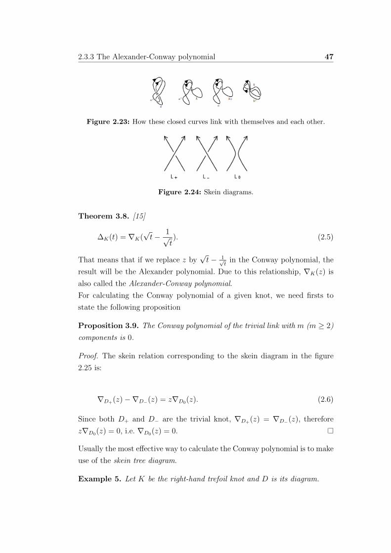
Example 6. The skein diagram for the Conway polynomial for the figure-

eight knot is the following:

Figure 2.27: Skein diagrams for the figure-eight knot.

Using the same calculation as above, we get:

∇K(z) = 1∇©(z) + z∇©©(z)− z2∇©(z) = 1− z2.

Therefore:

∆K(t) = 1 + (√t− 1√

t)2 = −t−1 + 3− t.

50 Knot invariants

4 The Jones revolution

4.1 Braids theory

In this section, we introduce some aspects of the theory of braids that will

be useful in explaining some developments in knot theory.

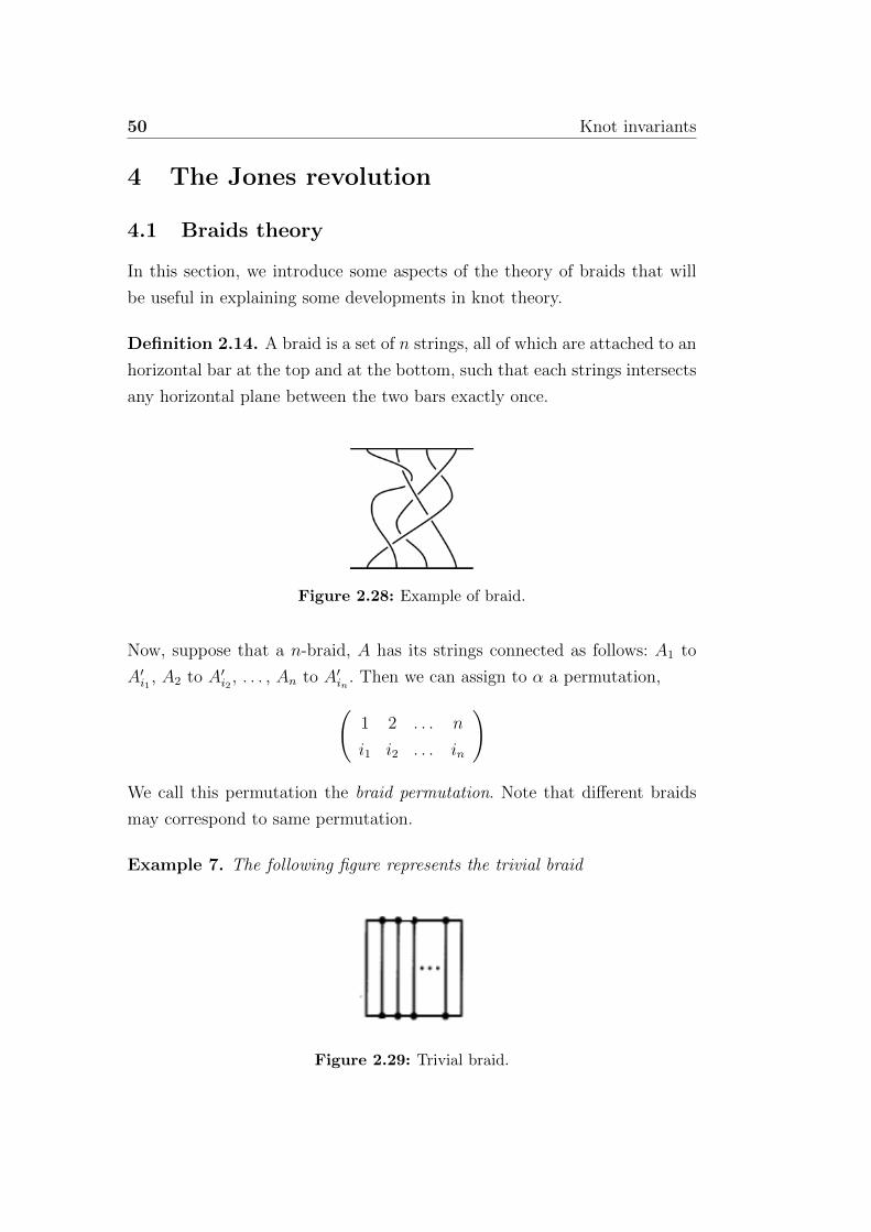
Definition 2.14. A braid is a set of n strings, all of which are attached to an

horizontal bar at the top and at the bottom, such that each strings intersects

any horizontal plane between the two bars exactly once.

Figure 2.28: Example of braid.

Now, suppose that a n-braid, A has its strings connected as follows: A1 to

A′i1 , A2 to A′i2 , . . . , An to A′in . Then we can assign to α a permutation,(1 2 . . . n

i1 i2 . . . in

)

We call this permutation the braid permutation. Note that different braids

may correspond to same permutation.

Example 7. The following figure represents the trivial braid

Figure 2.29: Trivial braid.

2.4.1 Braids theory 51

The trivial braid corresponds to the identity permutation,(1 2 . . . n

1 2 . . . n

)

Intuitively, two braids are said to be equivalent(in R3) if we can continuously

deform one to the other without causing any strings to intersect each other.

Proposition 4.1. If two braids are equivalent, they have the same permuta-

tion.

Example 8. In the figure 2.30 we can see an example of two equivalent

braids.

Figure 2.30: Two equivalent braids.

The braid permutation is (1 2 3

3 2 1

)The two braids are equivalent, then they have the same permutation. There-

fore the braid permutation is a braid invariant. This is the simplest braid

invariant.

The main result of this section is showing that existence of the braid group.

Suppose that B is the set of all braids with n strings. For two elements in

B, α and β, we can define a product by attaching the bottom bar of braid to

the upper bar of the other.

The resultant braid is called the product of α and β and is denoted by αβ. In

general, it is not true that αβ = βα, i.e. αβ and βα need not to be equivalent

braids.

Although not necessarily commutative, the product of braids is associative,

i.e.

(αβ)γ = α(βγ).

52 Knot invariants

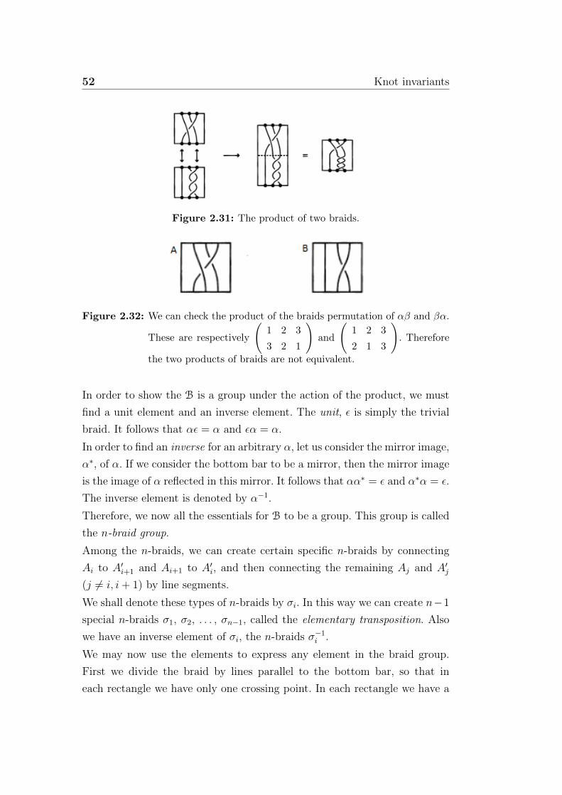
Figure 2.31: The product of two braids.

Figure 2.32: We can check the product of the braids permutation of αβ and βα.

These are respectively

(1 2 3

3 2 1

)and

(1 2 3

2 1 3

). Therefore

the two products of braids are not equivalent.

In order to show the B is a group under the action of the product, we must

find a unit element and an inverse element. The unit, ε is simply the trivial

braid. It follows that αε = α and εα = α.

In order to find an inverse for an arbitrary α, let us consider the mirror image,

α∗, of α. If we consider the bottom bar to be a mirror, then the mirror image

is the image of α reflected in this mirror. It follows that αα∗ = ε and α∗α = ε.

The inverse element is denoted by α−1.

Therefore, we now all the essentials for B to be a group. This group is called

the n-braid group.

Among the n-braids, we can create certain specific n-braids by connecting

Ai to A′i+1 and Ai+1 to A′i, and then connecting the remaining Aj and A′j

(j 6= i, i+ 1) by line segments.

We shall denote these types of n-braids by σi. In this way we can create n−1

special n-braids σ1, σ2, . . . , σn−1, called the elementary transposition. Also

we have an inverse element of σi, the n-braids σ−1i .

We may now use the elements to express any element in the braid group.

First we divide the braid by lines parallel to the bottom bar, so that in

each rectangle we have only one crossing point. In each rectangle we have a

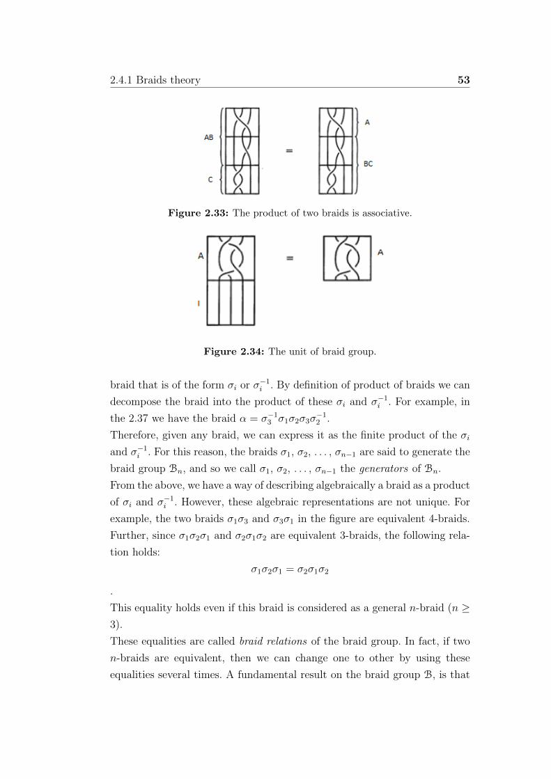
2.4.1 Braids theory 53

Figure 2.33: The product of two braids is associative.

Figure 2.34: The unit of braid group.

braid that is of the form σi or σ−1i . By definition of product of braids we can

decompose the braid into the product of these σi and σ−1i . For example, in

the 2.37 we have the braid α = σ−13 σ1σ2σ3σ−12 .

Therefore, given any braid, we can express it as the finite product of the σi

and σ−1i . For this reason, the braids σ1, σ2, . . . , σn−1 are said to generate the

braid group Bn, and so we call σ1, σ2, . . . , σn−1 the generators of Bn.

From the above, we have a way of describing algebraically a braid as a product

of σi and σ−1i . However, these algebraic representations are not unique. For

example, the two braids σ1σ3 and σ3σ1 in the figure are equivalent 4-braids.

Further, since σ1σ2σ1 and σ2σ1σ2 are equivalent 3-braids, the following rela-

tion holds:

σ1σ2σ1 = σ2σ1σ2

.

This equality holds even if this braid is considered as a general n-braid (n ≥3).

These equalities are called braid relations of the braid group. In fact, if two

n-braids are equivalent, then we can change one to other by using these

equalities several times. A fundamental result on the braid group B, is that

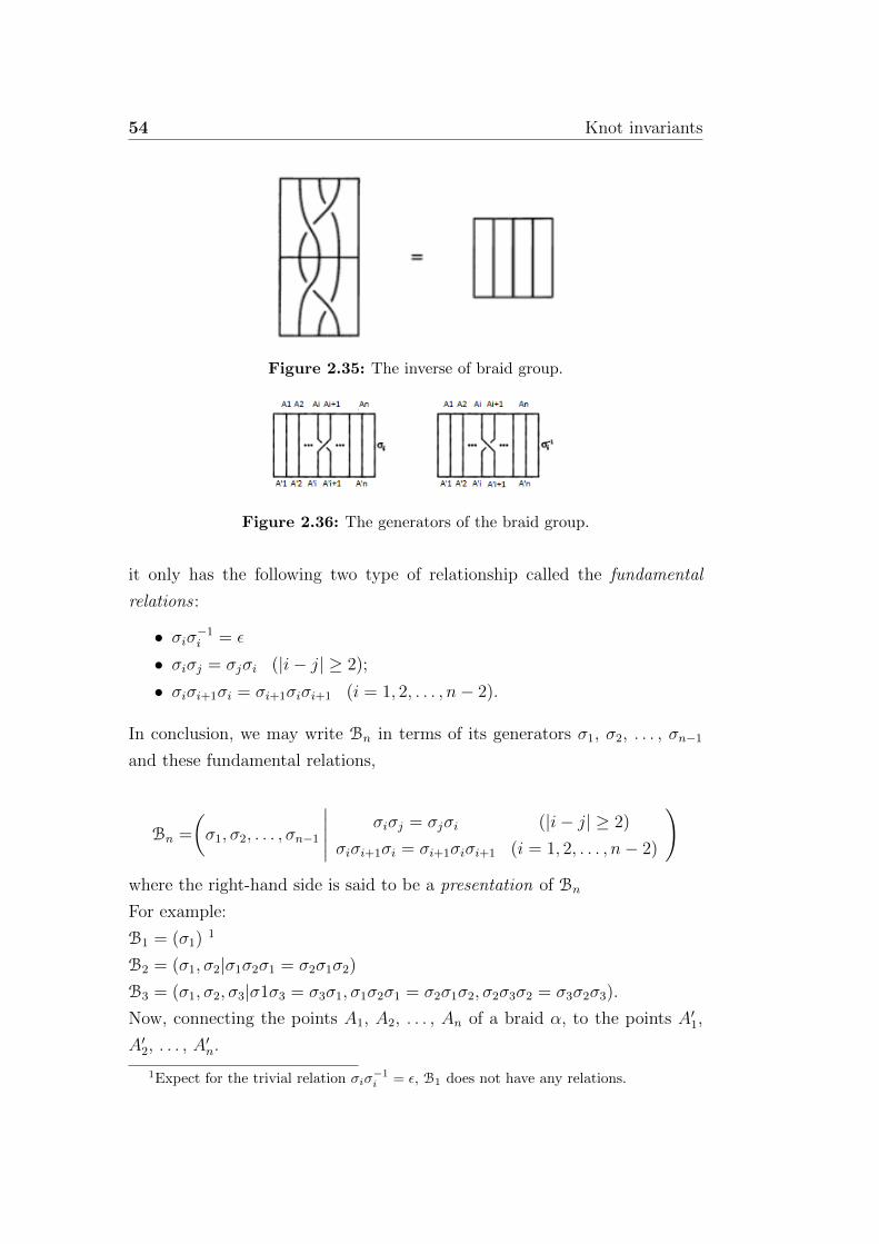
54 Knot invariants

Figure 2.35: The inverse of braid group.

Figure 2.36: The generators of the braid group.

it only has the following two type of relationship called the fundamental

relations :

• σiσ−1i = ε

• σiσj = σjσi (|i− j| ≥ 2);

• σiσi+1σi = σi+1σiσi+1 (i = 1, 2, . . . , n− 2).

In conclusion, we may write Bn in terms of its generators σ1, σ2, . . . , σn−1

and these fundamental relations,

Bn =

(σ1, σ2, . . . , σn−1

∣∣∣∣∣ σiσj = σjσi (|i− j| ≥ 2)

σiσi+1σi = σi+1σiσi+1 (i = 1, 2, . . . , n− 2)

)where the right-hand side is said to be a presentation of Bn

For example:

B1 = (σ1)1

B2 = (σ1, σ2|σ1σ2σ1 = σ2σ1σ2)

B3 = (σ1, σ2, σ3|σ1σ3 = σ3σ1, σ1σ2σ1 = σ2σ1σ2, σ2σ3σ2 = σ3σ2σ3).

Now, connecting the points A1, A2, . . . , An of a braid α, to the points A′1,

A′2, . . . , A′n.

1Expect for the trivial relation σiσ−1i = ε, B1 does not have any relations.

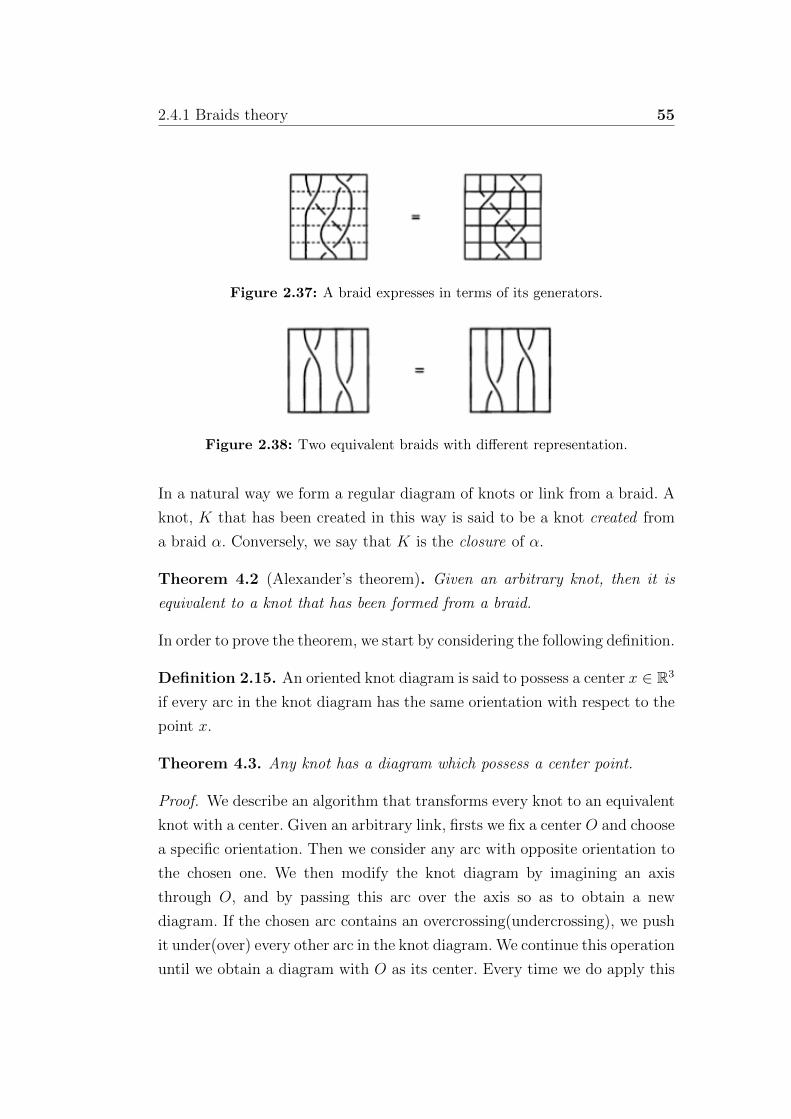
2.4.1 Braids theory 55

Figure 2.37: A braid expresses in terms of its generators.

Figure 2.38: Two equivalent braids with different representation.

In a natural way we form a regular diagram of knots or link from a braid. A

knot, K that has been created in this way is said to be a knot created from

a braid α. Conversely, we say that K is the closure of α.

Theorem 4.2 (Alexander’s theorem). Given an arbitrary knot, then it is

equivalent to a knot that has been formed from a braid.

In order to prove the theorem, we start by considering the following definition.

Definition 2.15. An oriented knot diagram is said to possess a center x ∈ R3

if every arc in the knot diagram has the same orientation with respect to the

point x.

Theorem 4.3. Any knot has a diagram which possess a center point.

Proof. We describe an algorithm that transforms every knot to an equivalent

knot with a center. Given an arbitrary link, firsts we fix a center O and choose

a specific orientation. Then we consider any arc with opposite orientation to

the chosen one. We then modify the knot diagram by imagining an axis

through O, and by passing this arc over the axis so as to obtain a new

diagram. If the chosen arc contains an overcrossing(undercrossing), we push

it under(over) every other arc in the knot diagram. We continue this operation

until we obtain a diagram with O as its center. Every time we do apply this

56 Knot invariants

Figure 2.39: Two equivalent braids with different representation.

Figure 2.40: The closure of braid.

move, the number of the of arcs that have opposite orientation with respect

to O is reduced by one. So this algorithm terminates, and since it terminates

only when there are no arcs with opposite orientation with respect to O, we

know that the knot obtained has a diagram with a center.

Now we can prove the Alexander’s theorem.

Proof. Given any knot, we can use the above theorem to modify it to a link

with a center O. We consider a perpendicular axis to the plane of the diagram

through the center O, and thus, the knot appears to be winding around this

axis. In fact, the knot can be viewed as being contained inside a tube or solid

torus T centered at O. Now we cut the torus along the ray from O through

its meridian and open it out, and obtain a cylinder which clearly contains a

braid.

Now, if two braids are equivalent, their knots, are also equivalent. However,

it is possible to obtain equivalent knots from the closure of nonequivalent

braids. For example the following braids are not equivalent, but their closure

are equivalent, to the trivial knot.

Having said that, we need to find out from which braids we can form equiv-

alent knots. Thus, we shall introduce the concept of M -equivalence between

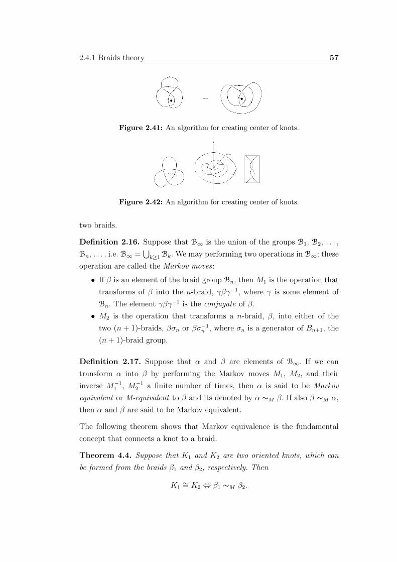
2.4.1 Braids theory 57

Figure 2.41: An algorithm for creating center of knots.

Figure 2.42: An algorithm for creating center of knots.

two braids.

Definition 2.16. Suppose that B∞ is the union of the groups B1, B2, . . . ,

Bn, . . . , i.e. B∞ =⋃k≥1Bk. We may performing two operations in B∞; these

operation are called the Markov moves :

• If β is an element of the braid group Bn, then M1 is the operation that

transforms of β into the n-braid, γβγ−1, where γ is some element of

Bn. The element γβγ−1 is the conjugate of β.

• M2 is the operation that transforms a n-braid, β, into either of the

two (n + 1)-braids, βσn or βσ−1n , where σn is a generator of Bn+1, the

(n+ 1)-braid group.

Definition 2.17. Suppose that α and β are elements of B∞. If we can

transform α into β by performing the Markov moves M1, M2, and their

inverse M−11 , M−1

2 a finite number of times, then α is said to be Markov

equivalent or M-equivalent to β and its denoted by α ∼M β. If also β ∼M α,

then α and β are said to be Markov equivalent.

The following theorem shows that Markov equivalence is the fundamental

concept that connects a knot to a braid.

Theorem 4.4. Suppose that K1 and K2 are two oriented knots, which can

be formed from the braids β1 and β2, respectively. Then

K1∼= K2 ⇔ β1 ∼M β2.

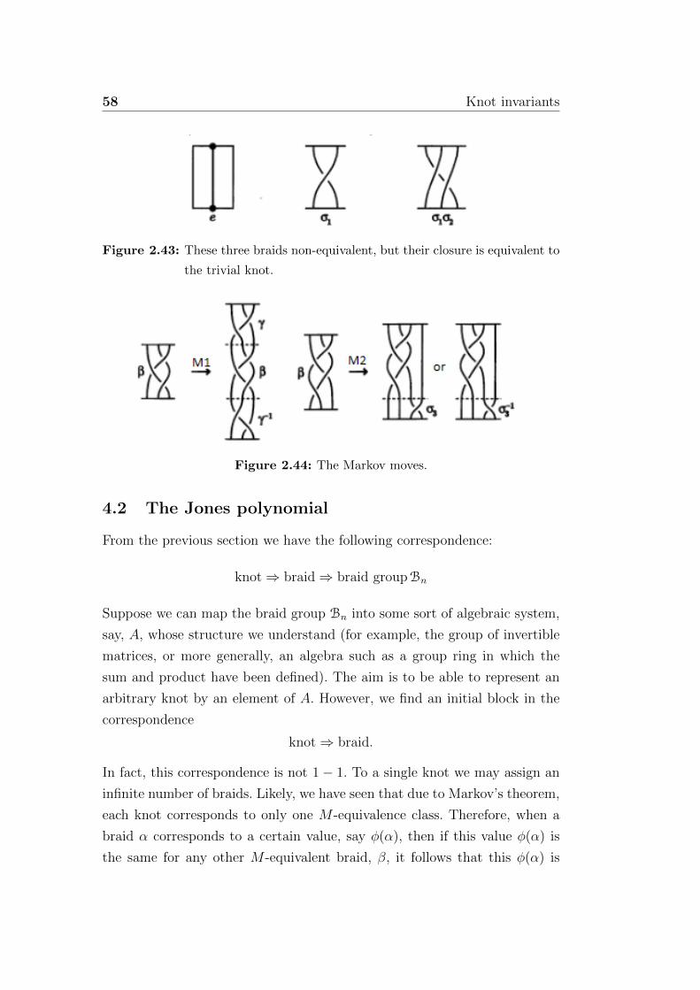
58 Knot invariants

Figure 2.43: These three braids non-equivalent, but their closure is equivalent to

the trivial knot.

Figure 2.44: The Markov moves.

4.2 The Jones polynomial

From the previous section we have the following correspondence:

knot⇒ braid⇒ braid groupBn

Suppose we can map the braid group Bn into some sort of algebraic system,

say, A, whose structure we understand (for example, the group of invertible

matrices, or more generally, an algebra such as a group ring in which the

sum and product have been defined). The aim is to be able to represent an

arbitrary knot by an element of A. However, we find an initial block in the

correspondence

knot⇒ braid.

In fact, this correspondence is not 1− 1. To a single knot we may assign an

infinite number of braids. Likely, we have seen that due to Markov’s theorem,

each knot corresponds to only one M -equivalence class. Therefore, when a

braid α corresponds to a certain value, say φ(α), then if this value φ(α) is

the same for any other M -equivalent braid, β, it follows that this φ(α) is

2.4.2 The Jones polynomial 59

an invariant of the knot Kα, formed from the braid α. So, from the first

condition of M -equivalence φ must have the same value for α and γαγ−1.

Now, if we want to represent the braid group by some algebraic structure, A,

it must have a similar structure to Bn. Further, A should have a simpler or

more restricted algebraic structure than Bn. Jones, accidentally, found that

one of the algebras, which he was studying for other purpose, had a structure

that resembled that of the braid group. He was able to define a function that

was invariant under both the Markov moves, M1 and M2. This function could

be written in terms of complex number q, and from this it was possible to

associate to each knot a complex polynomial. This polynomial is known as

the Jones polynomial. In this section we will study the Jones polynomial from

the point of view of knot theory, leaving the perspective of operator algebra

and quantum groups as application of knot theory.

Definition 2.18. Suppose K is a knot and D is a regular diagram for K.

Then the Jones polynomial of K, VK(t), can be define, uniquely, from the

following two axioms. The polynomial VK(t) is an invariant of K.

• If K is the trivial knot, then VK(t) = 1.

• Suppose that D+,D− and D0 are skein diagram (see fig.2.24), then the

following skein relation holds:

1

tVD+(t)− tVD−(t) = (

√t− 1√

t)VD0(t). (2.10)

The algorithm to calculate the Jones polynomial is completely analogous to

the one for the Alexander-Conway polynomial. We can write out the Jones

polynomial as the sum of the Jones polynomial of the trivial m-component

links, ©m (the result of using the skein tree diagram),

VK(t) = f1(t)V©(t) + f2(t)V©©(t) + · · ·+ fm(t)V©m(t). (2.11)

In the Alexander case, the above expression is superfluous, since the∇©m(t) =

0. But this is not the case for the Jones polynomial.

Theorem 4.5. For the trivial m-component link ©m,

V©m(t) = (−1)m−1(√t+

1√t)m−1 (2.12)

60 Knot invariants

Proof. We will proof the theorem by induction on m. If m = 1, then we have

the axiom 1. So let us assume for our induction hypothesis that the following

holds:

V©m−1(t) = (−1)m−2(√t+

1√t)m−2

Now consider the skein diagram as in figure, then since D+∼= D− ∼= ©m−1

and D0∼=©m, by the above induction hypothesis and the skein relation (in

the Jones definition),

(−1)m−2(√t+

√1√t)m−2 − t(−1)m−2(

√t+

1√t)m−2 =

= (√t− 1√

t)V©m(t).

Since the left-hand side of the above formula is

(−1)m−2(√t+

1√t)m−2(

1

t− t) =

= (−1)m−1(√t+

1√t)m−2(

√t+

1√t)(√t− 1√

t),

the result follows.

Now, let us calculate the Jones polynomial of some knots. For helping in the

calculation, let us write down the following equalities:

VD+(t) = t2VD−(t) + tzVD0(t)

VD−(t) = t−2VD+(t) + t−1zVD0(t)

where z = (√t− 1√

t).

Example 9. .

The skein tree diagram of the trefoil knot is:

It follows from the skein diagram that:

VK(t) = t2V©(t) + t3zV©©(t) + t2z2V©(t) = t+ t3 − t−4.

Example 10. It follows from the skein diagram of the figure-eight knot that:

VK(t) = t2V©(t) + tz[t−2V©©(t) + t−1zV©(t)] = t2 + t−2 − t− t−1 + 1.

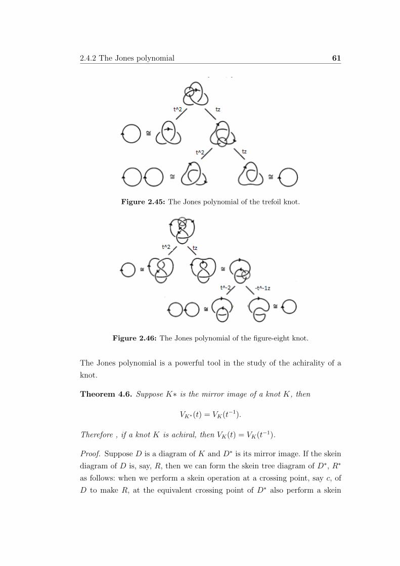
2.4.2 The Jones polynomial 61

Figure 2.45: The Jones polynomial of the trefoil knot.

Figure 2.46: The Jones polynomial of the figure-eight knot.

The Jones polynomial is a powerful tool in the study of the achirality of a

knot.

Theorem 4.6. Suppose K∗ is the mirror image of a knot K, then

VK∗(t) = VK(t−1).

Therefore , if a knot K is achiral, then VK(t) = VK(t−1).

Proof. Suppose D is a diagram of K and D∗ is its mirror image. If the skein

diagram of D is, say, R, then we can form the skein tree diagram of D∗, R∗

as follows: when we perform a skein operation at a crossing point, say c, of

D to make R, at the equivalent crossing point of D∗ also perform a skein

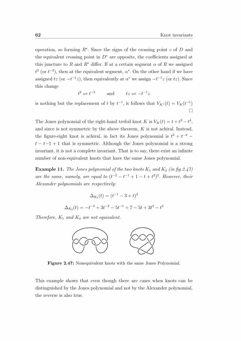
62 Knot invariants

operation, so forming R∗. Since the signs of the crossing point c of D and

the equivalent crossing point in D∗ are opposite, the coefficients assigned at

this juncture to R and R∗ differ. If at a certain segment α of R we assigned

t2 (or t−2), then at the equivalent segment, α∗. On the other hand if we have

assigned tz (or −t−1z), then equivalently at α∗ we assign −t−1z (or tz). Since

this change

t2 t−2 and tz −t−1z

is nothing but the replacement of t by t−1, it follows that VK∗(t) = VK(t−1)

The Jones polynomial of the right-hand trefoil knot K is VK(t) = t+ t3− t4,and since is not symmetric by the above theorem, K is not achiral. Instead,

the figure-eight knot is achiral, in fact its Jones polynomial is t2 + t−2 −t − t−1 + 1 that is symmetric. Although the Jones polynomial is a strong

invariant, it is not a complete invariant. That is to say, there exist an infinite

number of non-equivalent knots that have the same Jones polynomial.

Example 11. The Jones polynomial of the two knots K1 and K2 (in fig.2.47)

are the same, namely, are equal to (t−2 − t−1 + 1 − t + t2)2. However, their

Alexander polynomials are respectively:

∆K1(t) = (t−1 − 3 + t)2

∆K2(t) = −t−3 + 3t−2 − 5t−1 + 7− 5t+ 3t2 − t3

Therefore, K1 and K2 are not equivalent.

Figure 2.47: Nonequivalent knots with the same Jones Polynomial.

This example shows that even though there are cases when knots can be

distinguished by the Jones polynomial and not by the Alexander polynomial,

the reverse is also true.

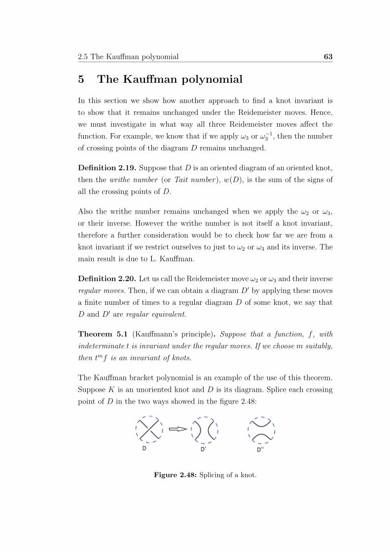
2.5 The Kauffman polynomial 63

5 The Kauffman polynomial

In this section we show how another approach to find a knot invariant is

to show that it remains unchanged under the Reidemeister moves. Hence,

we must investigate in what way all three Reidemeister moves affect the

function. For example, we know that if we apply ω3 or ω−13 , then the number

of crossing points of the diagram D remains unchanged.

Definition 2.19. Suppose that D is an oriented diagram of an oriented knot,

then the writhe number (or Tait number), w(D), is the sum of the signs of

all the crossing points of D.

Also the writhe number remains unchanged when we apply the ω2 or ω3,

or their inverse. However the writhe number is not itself a knot invariant,

therefore a further consideration would be to check how far we are from a

knot invariant if we restrict ourselves to just to ω2 or ω3 and its inverse. The

main result is due to L. Kauffman.

Definition 2.20. Let us call the Reidemeister move ω2 or ω3 and their inverse

regular moves. Then, if we can obtain a diagram D′ by applying these moves

a finite number of times to a regular diagram D of some knot, we say that

D and D′ are regular equivalent.

Theorem 5.1 (Kauffmann’s principle). Suppose that a function, f , with

indeterminate t is invariant under the regular moves. If we choose m suitably,

then tmf is an invariant of knots.

The Kauffman bracket polynomial is an example of the use of this theorem.

Suppose K is an unoriented knot and D is its diagram. Splice each crossing

point of D in the two ways showed in the figure 2.48:

Figure 2.48: Splicing of a knot.

64 Knot invariants

In order to define the Kauffman bracket polynomial we will use this process

of splicing a knot.

Theorem 5.2. Let D be an unoriented regular diagram o a knot or link

K. Then there exists a unique one-variable integer polynomial PD(A) that

satisfies the following conditions:

• PD(A) is invariant under regular equivalence.

• If D is the trivial projection (©) of the trivial knot, then

P©(A) = 1. (2.13)

• If D consists of two split diagram D1, D2, then

PD(A) = −(A2 + A−2)PD1(A)PD2(A). (2.14)

• Let D, D′ and D′′ be the skein diagrams given in the figure. Then the

following equality holds:

PD(A) = APD′(A) + A−1PD′′(A) (2.15)

PD(A) is called the Kauffman’s bracket polynomial Is important to under-

stand that this polynomial is defined on the knot diagram D. For example,

the first condition does not mean that PK(A) = 1, where K is the trivial knot.

Consider the trivial knot T as in the figure. In order to find PT (A) = −(A−3),

Figure 2.49: Two equivalent trivial knot.

we need to use the third condition to evaluate. Therefore, PD(A) is not in-

variant under the first Reidemeister move, ω1. However, according to the

Kauffman’s principle, it is possible to define an invariant from PD(A) that is

also invariant under ω1.

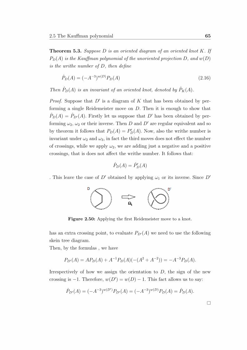
2.5 The Kauffman polynomial 65

Theorem 5.3. Suppose D is an oriented diagram of an oriented knot K. If

PD(A) is the Kauffman polynomial of the unoriented projection D, and w(D)

is the writhe number of D, then define

PD(A) = (−A−3)w(D)PD(A) (2.16)

Then PD(A) is an invariant of an oriented knot, denoted by PK(A).

Proof. Suppose that D′ is a diagram of K that has been obtained by per-

forming a single Reidemeister move on D. Then it is enough to show that

PD(A) = PD′(A). Firstly let us suppose that D′ has been obtained by per-

forming ω2, ω2 or their inverse. Then D and D′ are regular equivalent and so

by theorem it follows that PD(A) = P ′D(A). Now, also the writhe number is

invariant under ω2 and ω3, in fact the third moves does not effect the number

of crossings, while we apply ω2, we are adding just a negative and a positive

crossings, that is does not affect the writhe number. It follows that:

PD(A) = P ′D(A)

. This leave the case of D′ obtained by applying ω1 or its inverse. Since D′

Figure 2.50: Applying the first Reidemeister move to a knot.

has an extra crossing point, to evaluate PD′(A) we need to use the following

skein tree diagram.

Then, by the formulas , we have

PD′(A) = APD(A) + A−1PD(A)(−(A2 + A−2)) = −A−3PD(A).

Irrespectively of how we assign the orientation to D, the sign of the new

crossing is −1. Therefore, w(D′) = w(D)− 1. This fact allows us to say:

PD′(A) = (−A−3)w(D′)PD′(A) = (−A−3)w(D)PD(A) = PD(A).

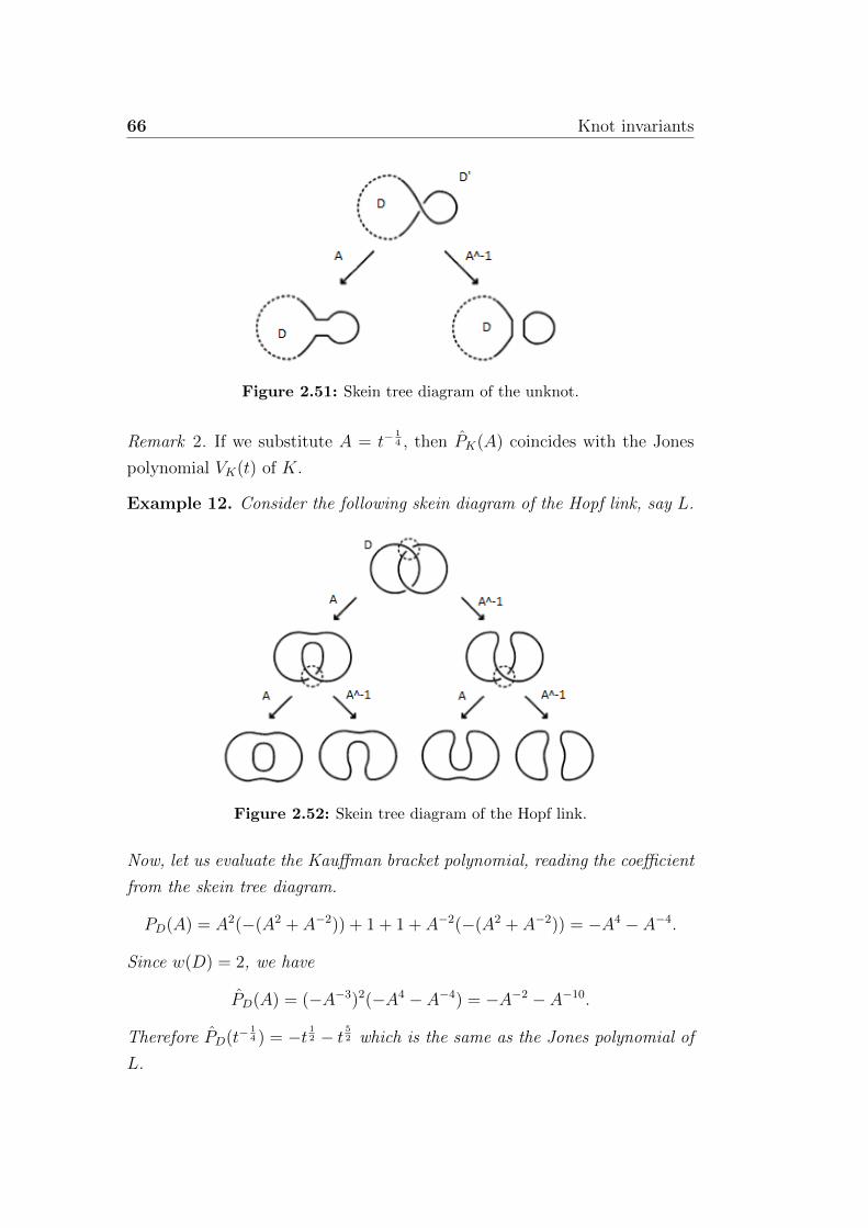
66 Knot invariants

Figure 2.51: Skein tree diagram of the unknot.

Remark 2. If we substitute A = t−14 , then PK(A) coincides with the Jones

polynomial VK(t) of K.

Example 12. Consider the following skein diagram of the Hopf link, say L.

Figure 2.52: Skein tree diagram of the Hopf link.

Now, let us evaluate the Kauffman bracket polynomial, reading the coefficient

from the skein tree diagram.

PD(A) = A2(−(A2 + A−2)) + 1 + 1 + A−2(−(A2 + A−2)) = −A4 − A−4.

Since w(D) = 2, we have

PD(A) = (−A−3)2(−A4 − A−4) = −A−2 − A−10.

Therefore PD(t−14 ) = −t 12 − t 52 which is the same as the Jones polynomial of

L.

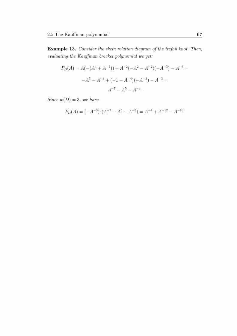
2.5 The Kauffman polynomial 67

Example 13. Consider the skein relation diagram of the trefoil knot. Then,

evaluating the Kauffman bracket polynomial we get:

PD(A) = A(−(A4 + A−4)) + A−2(−A2 − A−2)(−A−3)− A−3 =

−A5 − A−3 + (−1− A−4)(−A−3)− A−3 =

A−7 − A5 − A−3.

Since w(D) = 3, we have

PD(A) = (−A−3)3(A−7 − A5 − A−3) = A−4 + A−12 − A−16.

Chapter 3

Knot theory: Application

1 Knot theory in chemistry

In this chapter the different application of knot theory are introduced. First,

let us have a look of what means molecular chirality and how the knot the-

ory can be useful in determining when a molecular is chiral or not. Later

on we will see how the Yang-Baxter equation is related to the braids group,

and so with the knots. In the end another important knot theory’s applica-

tion is given, this time in biology. In fact, it was discovered that the DNA-

recombination can be described as a mathematical model, know as tangles

model.

1.1 The Molecular chirality

How would you like to live in Looking-glass

House, Kitty? I wonder if they’d give you

milk, there? Perhaps Looking-glass milk isn’t

good to drink...

Lewis Carroll, Through the looking-glass

One of the most important characteristics of a knot is its chirality. During

the years, all the knots theorists have tried to find a way to determinate it.

As we said previously, the Jones polynomial was the key for this problem.

70 Knot theory: Application

The word chiral derives from the ancient greek word χειρ which means

”hand”. Since one hand is always different from its mirror image, this word

is used to indicate an object who cannot be superposable onto its image in

the mirror. The chirality is really important in chemistry, since a molecule

and its mirror image can have different properties. Two mirror images of a

chiral molecule are called enantiomers.

An example is the limonene, C10H16. The L-limonene (L stands for levo, the

left-handed enantiomer) has a harsh lemon scent, while the D-limonene (D

stands for dextro the right-handed enantiomer) has a more pleasing orange

scent.

In the pharmaceutical industry this matter can make the difference. A chi-

ral drug could have two different effects: one of the enantiomer produces

the desired effect while the other one has a side effect that could outweigh

the benefit of the wanted effect. In 1960’s the drug Thalidomide was given

to pregnant women to avoid the morning sickness. It causes, besides the

reducing of sickness, also birth defect. This happens because, while the L-

Thalidomide was making the mother feeling better, the D-Thalidomide was

causing damage to the fetus. Therefore if a drug is known to be chiral, the

pharmaceutical industry can choose to manufacture just the preferred form

in order to minimize the side effect and maximize effectiveness. This is costly

since most methods of molecular synthesis do not distingue between different

chirality. Sadly, as the Thalidomide, in most of the cases the wrong chirality

produces negative effect on human body.

Definition 3.1. A molecule is said to be chemically achiral if it can be

changed into its mirror image. Otherwise is said to be chemically chiral.

This is the definition given in chemistry. In mathematics there are other two

definitions, geometrical chirality and topological chirality according to the

characteristics of the molecule, respectively rigid or flexible.

Definition 3.2. A molecule is said to be geometrical achiral if, as a rigid

object, can be superposable on its mirror image. Otherwise is said to be

geometric chiral.

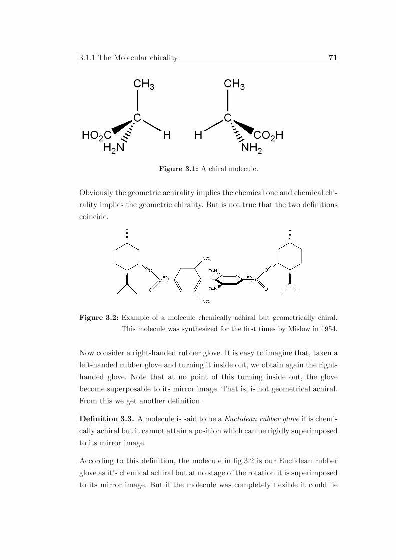
3.1.1 The Molecular chirality 71

Figure 3.1: A chiral molecule.

Obviously the geometric achirality implies the chemical one and chemical chi-

rality implies the geometric chirality. But is not true that the two definitions

coincide.

Figure 3.2: Example of a molecule chemically achiral but geometrically chiral.

This molecule was synthesized for the first times by Mislow in 1954.

Now consider a right-handed rubber glove. It is easy to imagine that, taken a

left-handed rubber glove and turning it inside out, we obtain again the right-

handed glove. Note that at no point of this turning inside out, the glove

become superposable to its mirror image. That is, is not geometrical achiral.

From this we get another definition.

Definition 3.3. A molecule is said to be a Euclidean rubber glove if is chemi-

cally achiral but it cannot attain a position which can be rigidly superimposed

to its mirror image.

According to this definition, the molecule in fig.3.2 is our Euclidean rubber

glove as it’s chemical achiral but at no stage of the rotation it is superimposed

to its mirror image. But if the molecule was completely flexible it could lie

72 Knot theory: Application

in the plane and become superimposed to its mirror image. Similarly for

the rubber glove. However the natural characteristic of this object does not

allow a completely flexibility. Since the possibility that a completely flexible

molecule exists another definition is required.

Definition 3.4. A molecule is said to be a topologically rubber glove if is

chemically achiral but it cannot be deformed to a position in which is super-

imposed to its mirror image.

Figure 3.3: This molecule and its mirror image are example of topological rubber

glove molecule.

Summarizing, the Euclidean and topological rubber gloves are examples of

molecules that are chemically achiral but not geometrically achiral.

Since the geometrical chirality considers molecules as rigid objects, and in

nature molecules are not rigid objects it is worth to consider the case of

molecules as completely flexible objects.

Definition 3.5. A molecule is said to be topologically achiral if, assuming

complete flexibility, there is a deformation which takes it to its mirror image.

Otherwise it is said to be topologically chiral.

3.1.2 Graphs 73

If a molecule is topologically chiral no deformation can be made to make it

become its mirror image, indeed is also chemically chiral. Otherwise if it is

chemical achiral, then it is also topologically achiral.

The following scheme summarizes the relationship between the previous three

definition:

topologically chirality → chemical chirality → geometrical chirality.

geometrical achirality → chemical achirality → topologically achirality.

1.2 Graphs

Let V be a finite set, and denote by

E(V ) = {{u, v}|u, v ∈ V, u 6= v}

. the subsets of V with two distinct elements.

Definition 3.6. A pair G = (V,E) with E = E(V ) is called a graph (on V ).

The elements of V are the vertices of G, and those of E the edges of G. The

vertex set of a graph G is denoted by VG and its edge set by EG. Therefore

G = (VG, EG).

Sometimes graphs are also called simple graphs ; vertices are called nodes or

points ; edges are called lines or links. A pair {u, v} is usually written simply

as uv. Notice that then uv = vu. In order to simplify notations, we also write

vG and eG instead of v ∈ VG and e ∈ EG.

For a graph G, we denote

νG = |VG| and εG = |EG|.

The number νG of the vertices is called the order of G, and εG is called the

size of G. For an edge e = uv ∈ G, the vertices u and v are its ends. Vertices

u and v are adjacent or neighbors, if uv ∈ G. Two edges e1 = uv and e2 = uw

having a common end, are adjacent with each other.

A graph G can be represented as a plane figure by drawing a line (or a

curve) between the points u and v (representing vertices) if e = uv is an

edge of G. The figure 3.4 is a geometric representation of the graph G with

VG = {v1, v2, v3, v4, v5, v6} and EG = {v1v2, v1v3, v2v3, v2v4, v5v6}.

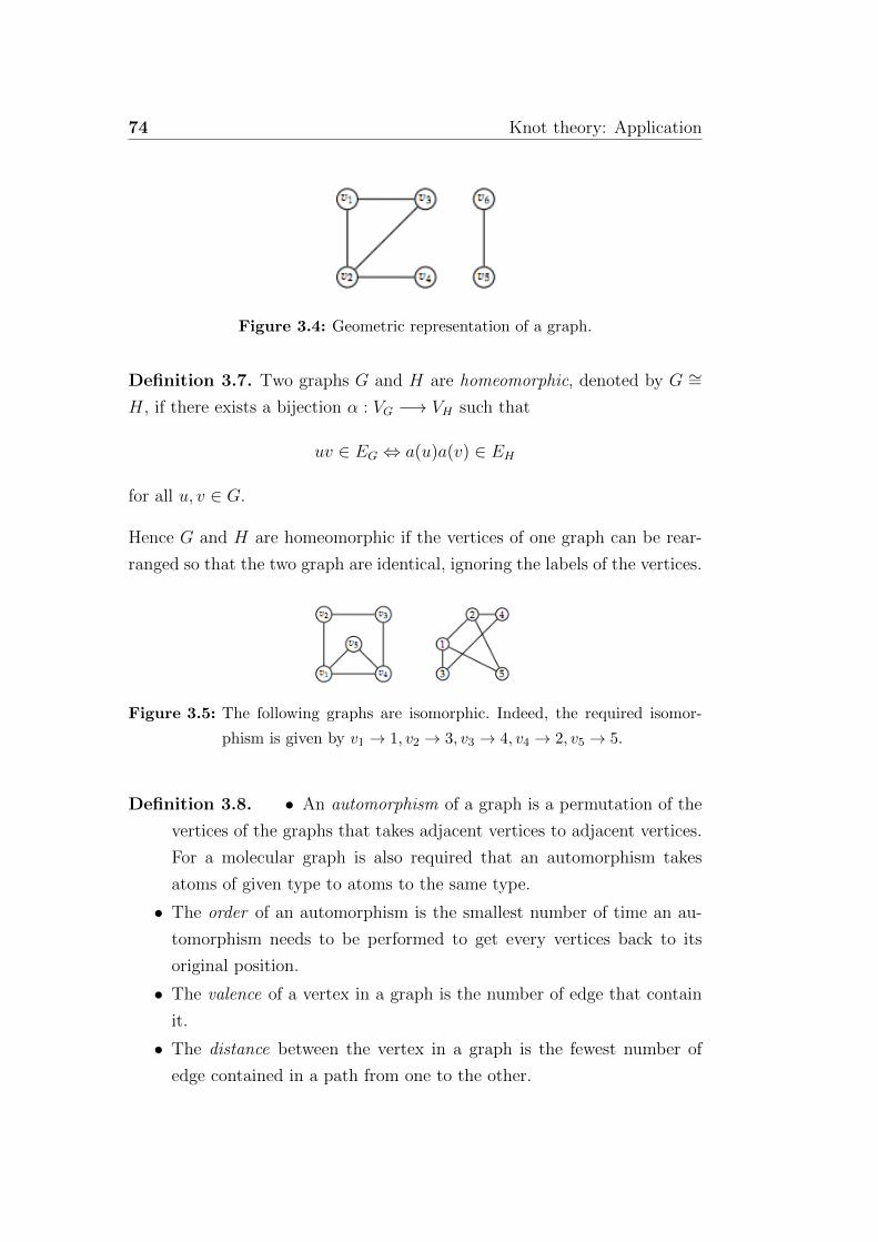
74 Knot theory: Application

Figure 3.4: Geometric representation of a graph.

Definition 3.7. Two graphs G and H are homeomorphic, denoted by G ∼=H, if there exists a bijection α : VG −→ VH such that

uv ∈ EG ⇔ a(u)a(v) ∈ EH

for all u, v ∈ G.

Hence G and H are homeomorphic if the vertices of one graph can be rear-

ranged so that the two graph are identical, ignoring the labels of the vertices.

Figure 3.5: The following graphs are isomorphic. Indeed, the required isomor-

phism is given by v1 → 1, v2 → 3, v3 → 4, v4 → 2, v5 → 5.

Definition 3.8. • An automorphism of a graph is a permutation of the

vertices of the graphs that takes adjacent vertices to adjacent vertices.

For a molecular graph is also required that an automorphism takes

atoms of given type to atoms to the same type.

• The order of an automorphism is the smallest number of time an au-

tomorphism needs to be performed to get every vertices back to its

original position.

• The valence of a vertex in a graph is the number of edge that contain

it.

• The distance between the vertex in a graph is the fewest number of

edge contained in a path from one to the other.

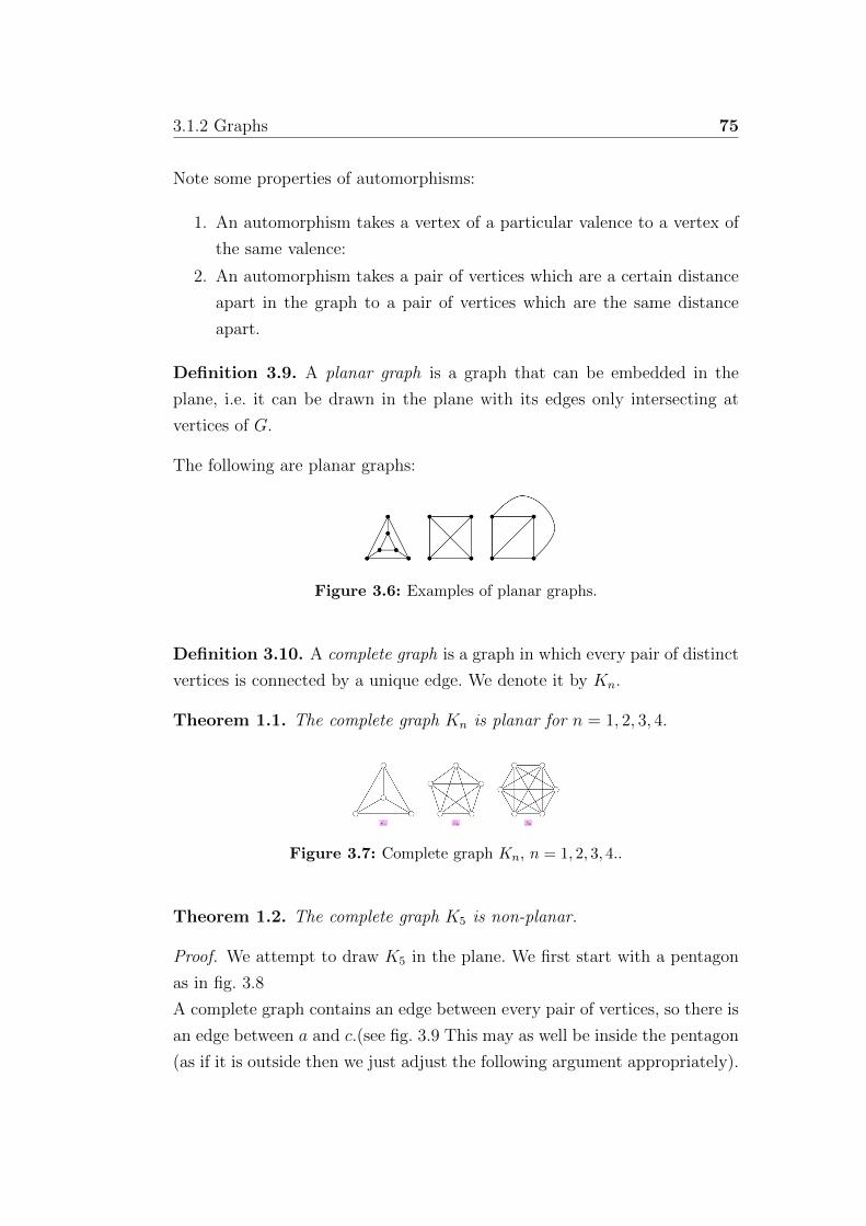
3.1.2 Graphs 75

Note some properties of automorphisms:

1. An automorphism takes a vertex of a particular valence to a vertex of

the same valence:

2. An automorphism takes a pair of vertices which are a certain distance

apart in the graph to a pair of vertices which are the same distance

apart.

Definition 3.9. A planar graph is a graph that can be embedded in the

plane, i.e. it can be drawn in the plane with its edges only intersecting at

vertices of G.

The following are planar graphs:

Figure 3.6: Examples of planar graphs.

Definition 3.10. A complete graph is a graph in which every pair of distinct

vertices is connected by a unique edge. We denote it by Kn.

Theorem 1.1. The complete graph Kn is planar for n = 1, 2, 3, 4.

Figure 3.7: Complete graph Kn, n = 1, 2, 3, 4..

Theorem 1.2. The complete graph K5 is non-planar.

Proof. We attempt to draw K5 in the plane. We first start with a pentagon

as in fig. 3.8

A complete graph contains an edge between every pair of vertices, so there is

an edge between a and c.(see fig. 3.9 This may as well be inside the pentagon

(as if it is outside then we just adjust the following argument appropriately).

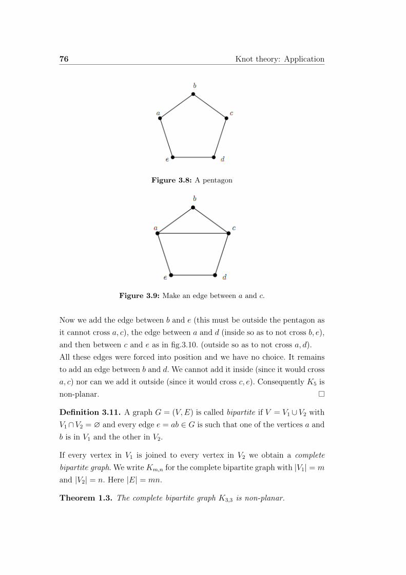
76 Knot theory: Application

Figure 3.8: A pentagon

Figure 3.9: Make an edge between a and c.

Now we add the edge between b and e (this must be outside the pentagon as

it cannot cross a, c), the edge between a and d (inside so as to not cross b, e),

and then between c and e as in fig.3.10. (outside so as to not cross a, d).

All these edges were forced into position and we have no choice. It remains

to add an edge between b and d. We cannot add it inside (since it would cross

a, c) nor can we add it outside (since it would cross c, e). Consequently K5 is

non-planar.

Definition 3.11. A graph G = (V,E) is called bipartite if V = V1 ∪ V2 with

V1∩V2 = ∅ and every edge e = ab ∈ G is such that one of the vertices a and

b is in V1 and the other in V2.

If every vertex in V1 is joined to every vertex in V2 we obtain a complete

bipartite graph. We write Km,n for the complete bipartite graph with |V1| = m

and |V2| = n. Here |E| = mn.

Theorem 1.3. The complete bipartite graph K3,3 is non-planar.

3.1.2 Graphs 77

Figure 3.10: The edge betwenn b and d cannot be added it inside (since it would

cross a, c) nor can we add it outside (since it would cross c, e).

Figure 3.11: The complete bipartite graph K3,3

Proof. Let V1 = a, b, c and V2 = x, y, z and draw a hexagonal circuit: a →x→ b→ y → c→ z → a

The proof is completed by observing that two of the edges a, y, b, z or c, x

must both lie inside or both outside the hexagon and hence must cross.

Theorem 1.4. (Kuratowski 1930) A graph is non-planar if and only if it

contains a subgraph that is homeomorphic to either K5 or K3,3.

This result is fundamental in graph theory since it allows us to see whether or

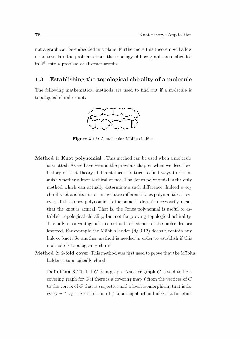
78 Knot theory: Application

not a graph can be embedded in a plane. Furthermore this theorem will allow

us to translate the problem about the topology of how graph are embedded

in R3 into a problem of abstract graphs.

1.3 Establishing the topological chirality of a molecule

The following mathematical methods are used to find out if a molecule is

topological chiral or not.

Figure 3.12: A molecular Mobius ladder.

Method 1: Knot polynomial . This method can be used when a molecule

is knotted. As we have seen in the previous chapter when we described

history of knot theory, different theorists tried to find ways to distin-

guish whether a knot is chiral or not. The Jones polynomial is the only

method which can actually determinate such difference. Indeed every

chiral knot and its mirror image have different Jones polynomials. How-

ever, if the Jones polynomial is the same it doesn’t necessarily mean

that the knot is achiral. That is, the Jones polynomial is useful to es-

tablish topological chirality, but not for proving topological achirality.

The only disadvantage of this method is that not all the molecules are

knotted. For example the Mobius ladder (fig.3.12) doesn’t contain any

link or knot. So another method is needed in order to establish if this

molecule is topologically chiral.

Method 2: 2-fold cover This method was first used to prove that the Mobius

ladder is topologically chiral.

Definition 3.12. Let G be a graph. Another graph C is said to be a

covering graph for G if there is a covering map f from the vertices of C

to the vertex of G that is surjective and a local isomorphism, that is for

every v ∈ VC the restriction of f to a neighborhood of v is a bijection

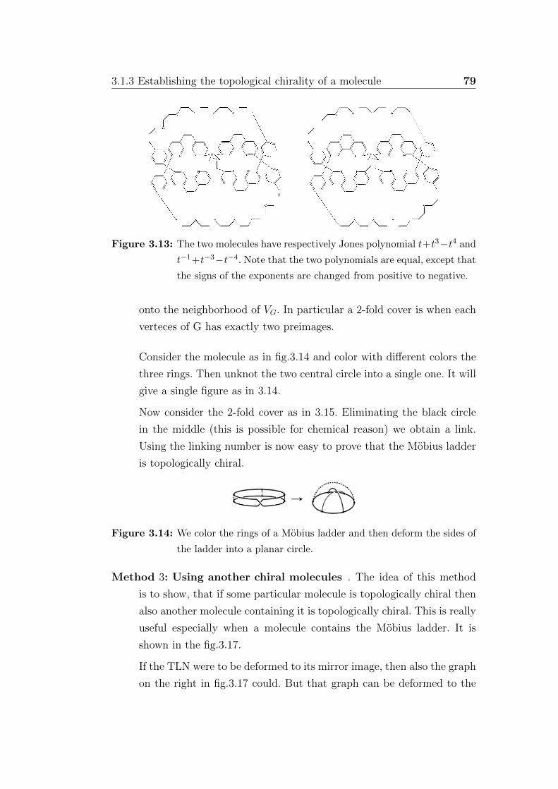
3.1.3 Establishing the topological chirality of a molecule 79

Figure 3.13: The two molecules have respectively Jones polynomial t+t3−t4 and

t−1+t−3−t−4. Note that the two polynomials are equal, except that

the signs of the exponents are changed from positive to negative.

onto the neighborhood of VG. In particular a 2-fold cover is when each

verteces of G has exactly two preimages.

Consider the molecule as in fig.3.14 and color with different colors the

three rings. Then unknot the two central circle into a single one. It will

give a single figure as in 3.14.

Now consider the 2-fold cover as in 3.15. Eliminating the black circle

in the middle (this is possible for chemical reason) we obtain a link.

Using the linking number is now easy to prove that the Mobius ladder

is topologically chiral.

Figure 3.14: We color the rings of a Mobius ladder and then deform the sides of

the ladder into a planar circle.

Method 3: Using another chiral molecules . The idea of this method

is to show, that if some particular molecule is topologically chiral then

also another molecule containing it is topologically chiral. This is really

useful especially when a molecule contains the Mobius ladder. It is

shown in the fig.3.17.

If the TLN were to be deformed to its mirror image, then also the graph

on the right in fig.3.17 could. But that graph can be deformed to the

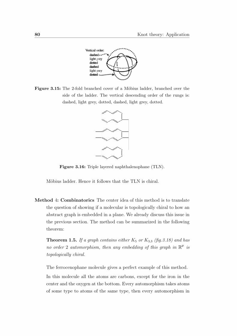
80 Knot theory: Application

Figure 3.15: The 2-fold branched cover of a Mobius ladder, branched over the

side of the ladder. The vertical descending order of the rungs is:

dashed, light grey, dotted, dashed, light grey, dotted.

Figure 3.16: Triple layered naphthalenophane (TLN).

Mobius ladder. Hence it follows that the TLN is chiral.

Method 4: Combinatorics The center idea of this method is to translate

the question of showing if a molecular is topologically chiral to how an

abstract graph is embedded in a plane. We already discuss this issue in

the previous section. The method can be summarized in the following

theorem:

Theorem 1.5. If a graph contains either K5 or K3,3 (fig.3.18) and has

no order 2 automorphism, then any embedding of this graph in R3 is

topologically chiral.

The ferrocenophane molecule gives a perfect example of this method.

In this molecule all the atoms are carbons, except for the iron in the

center and the oxygen at the bottom. Every automorphism takes atoms

of some type to atoms of the same type, then every automorphism in

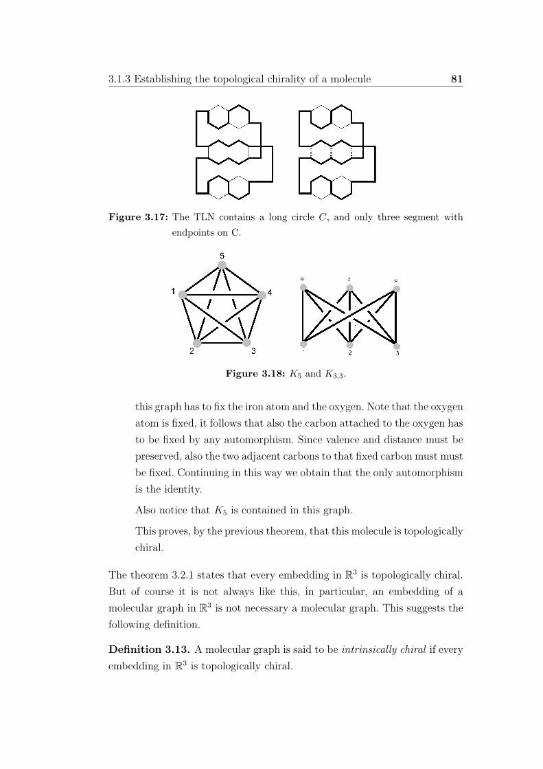
3.1.3 Establishing the topological chirality of a molecule 81

Figure 3.17: The TLN contains a long circle C, and only three segment with

endpoints on C.

Figure 3.18: K5 and K3,3.

this graph has to fix the iron atom and the oxygen. Note that the oxygen

atom is fixed, it follows that also the carbon attached to the oxygen has

to be fixed by any automorphism. Since valence and distance must be

preserved, also the two adjacent carbons to that fixed carbon must must

be fixed. Continuing in this way we obtain that the only automorphism

is the identity.

Also notice that K5 is contained in this graph.

This proves, by the previous theorem, that this molecule is topologically

chiral.

The theorem 3.2.1 states that every embedding in R3 is topologically chiral.

But of course it is not always like this, in particular, an embedding of a

molecular graph in R3 is not necessary a molecular graph. This suggests the

following definition.

Definition 3.13. A molecular graph is said to be intrinsically chiral if every

embedding in R3 is topologically chiral.

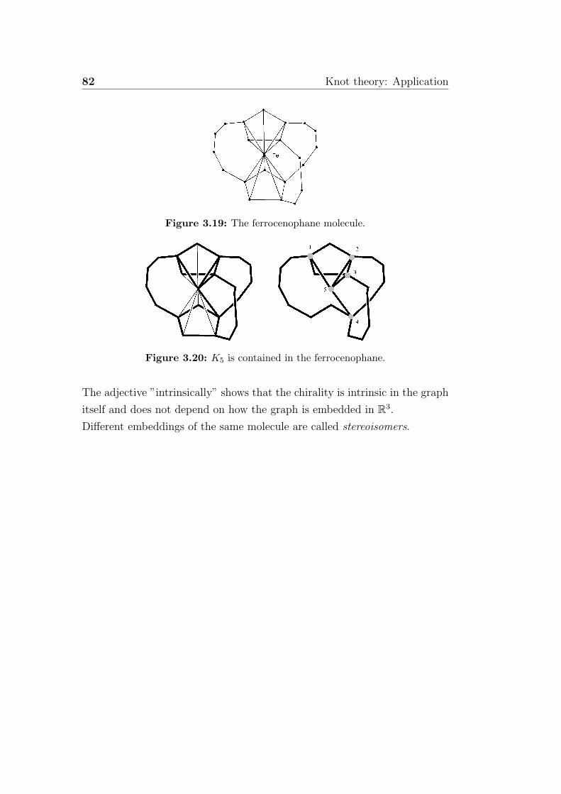
82 Knot theory: Application

Figure 3.19: The ferrocenophane molecule.

Figure 3.20: K5 is contained in the ferrocenophane.

The adjective ”intrinsically” shows that the chirality is intrinsic in the graph

itself and does not depend on how the graph is embedded in R3.

Different embeddings of the same molecule are called stereoisomers.

3.2 Knots and Physics 83

2 Knots and Physics

Statistic mechanics is a branch of physics that tries to understand, using

statistical methods, macroscopic properties by looking at microscopic prop-

erties. The easiest example is trying to understand what happens to water in

a kettle when we bring it to a boil by looking at how the molecules interact.

Statistical mechanics together with quantum mechanics formed the base for

the study of physics of matter. In general, the constituent of matter, even if

we assume they obey the principles of dynamics, have extremely complicated

means of motion, so modeling these motion is the most difficult problem in

physics. In order to find a reasonable successful method around this problem,

an ideal realization of matter, a model, has been formed. In order to give a

mathematical meaning to these realization we define a function Z called the

partition function,

Z =∑σ

exp(−E(σ)

kT)

in which σ is a state of the particular model, E(σ) is the total energy of this

state, T is the absolute temperature and k is the Boltzmann’s constant. If the

partition function of a model can be derived exactly, then this model is said

to be exactly solvable. The idea of the statistical mechanical approach to knot

invariants is to construct lattice models whose partition functions are taken

to be knot invariants. Specifically, starting from a given knot projection, we

can construct a two-dimensional lattice and a lattice model on this lattice. If

model parameters are chosen such that the partition function of the model

remains invariant when the knot (and the lattice) is deformed, the partition

function is a knot invariant by its very definition.

There are generally three different kinds of lattice models: The vertex models,

the closely related IRF (interaction round a face) models and the spin models.

The firsts two models are the most general and have been widely studied in

connection with quantum groups. Instead very few knot invariants seem to

admit a spin model description, and no clear connection with quantum groups

is known in general.

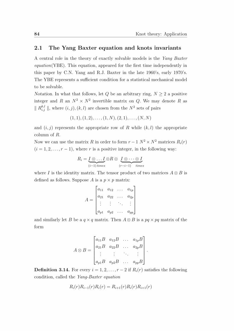
84 Knot theory: Application

2.1 The Yang Baxter equation and knots invariants

A central role in the theory of exactly solvable models is the Yang Baxter

equation(YBE). This equation, appeared for the first time independently in

this paper by C.N. Yang and R.J. Baxter in the late 1960’s, early 1970’s.

The YBE represents a sufficient condition for a statistical mechanical model

to be solvable.

Notation. In what that follows, let Q be an arbitrary ring, N ≥ 2 a positive

integer and R an N2 × N2 invertible matrix on Q. We may denote R as

‖ Rk,li,j ‖, where (i, j), (k, l) are chosen from the N2 sets of pairs

(1, 1), (1, 2), . . . , (1, N), (2, 1), . . . , (N,N)

and (i, j) represents the appropriate row of R while (k, l) the appropriate

column of R.

Now we can use the matrix R in order to form r− 1 N2×N2 matrices Ri(r)

(i = 1, 2, . . . , r − 1), where r is a positive integer, in the following way:

Ri = I ⊗ . . . I︸ ︷︷ ︸(i−1) times

⊗R⊗ I ⊗ · · · ⊗ I︸ ︷︷ ︸(r−i−1) times

where I is the identity matrix. The tensor product of two matrices A⊗B is

defined as follows. Suppose A is a p× p matrix:

A =

a11 a12 . . . a1p

a21 a22 . . . a2p...

.... . .

...

ap1 ap2 . . . app

and similarly let B be a q× q matrix. Then A⊗B is a pq× pq matrix of the

form

A⊗B =

a11B a12B . . . a1pB

a21B a22B . . . a2pB...

.... . .

...

ap1B ap2B . . . appB

.Definition 3.14. For every i = 1, 2, . . . , r− 2 if Ri(r) satisfies the following

condition, called the Yang-Baxter equation

Ri(r)Ri−1(r)Ri(r) = Ri+1(r)Ri(r)Ri+1(r)

3.2.1 The Yang Baxter equation and knots invariants 85

then R1(r), R2(r), . . . , Rr−1(r) are called the Yang-Baxter operators.

Definition 3.15. Let a, b ∈ Q∗. Let µ be a N2 × N2 diagonal matrix with

trace µ1, µ2, . . . , µN . A set {R, µ, a, b} is called an enhanced Yang Baxter

operators [19] if it satisfies:

• For any i, j, k, l ∈ 1, . . . , N , (µiµj − µjµi)Rk,li,j = 0

• 1.∑N

j=1Rk,li,jµj = abδki

2.∑N

j=1R−1k,l

i,jµj = a−1bδki

(Here δki is the Kronecker symbol: δki = 1, δki = 0 for k 6= j)

µ ⊗ µ commute with R if and only if µ ⊗ µ commute with R−1. Therefore,

the first condition in def.3.18 implies that for i, j, k, l µiµj −µkµl)R−1k,li,j = 0.

The secondo condition implies that the product of the square matrix Rk,li,j

with the column µ1

...

µN

is equal to the constant column ab

...

ab

Recall that the braid group Br (see chapter 2.4.1) has the following presen-

tation:

Br =

(σ1, σ2, . . . , σn−1

∣∣∣∣∣ σiσj = σjσi (|i− j| ≥ 2)

σiσi+1σi = σi+1σiσi+1 (i = 1, 2, . . . , n− 2)

)Notice that, by definition

Ri(r)Rj(r) = Rj(r)Ri(r) for |i− | ≥ 2.

Therefore, there is a unique homomorphism

bR : Bn →MN2×N2

which transforms σi ∈ Br into Ri for all i. Then, every element of Br, say

β = σε1j1 (r)σε2j2 (r) . . . σεmjm (r), can be represented by an N r ×N r matrix, i.e.

bR(β) = Rε1j1

(r)Rε2j2

(r) . . . Rεmjm

(r).

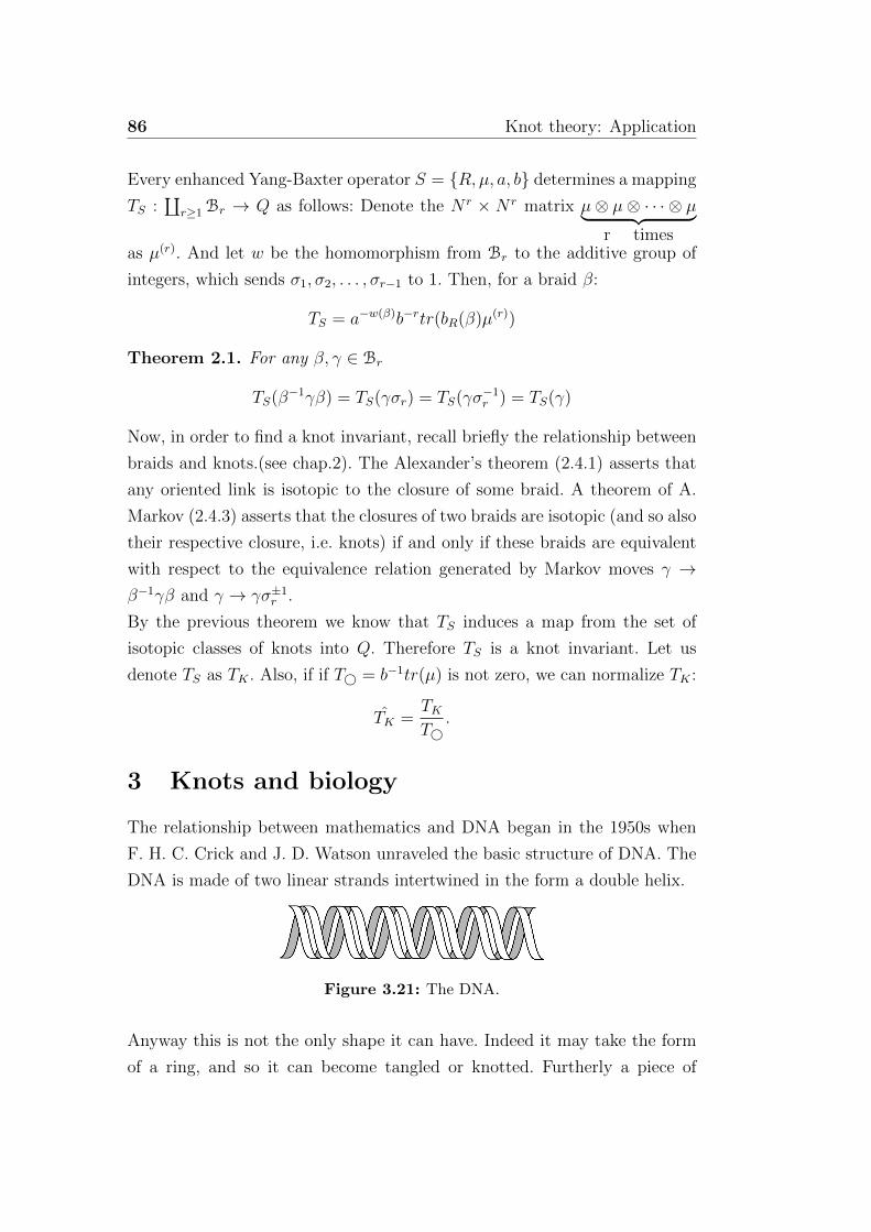
86 Knot theory: Application

Every enhanced Yang-Baxter operator S = {R, µ, a, b} determines a mapping

TS :∐

r≥1Br → Q as follows: Denote the N r × N r matrix µ⊗ µ⊗ · · · ⊗ µ︸ ︷︷ ︸r times

as µ(r). And let w be the homomorphism from Br to the additive group of

integers, which sends σ1, σ2, . . . , σr−1 to 1. Then, for a braid β:

TS = a−w(β)b−rtr(bR(β)µ(r))

Theorem 2.1. For any β, γ ∈ Br

TS(β−1γβ) = TS(γσr) = TS(γσ−1r ) = TS(γ)

Now, in order to find a knot invariant, recall briefly the relationship between

braids and knots.(see chap.2). The Alexander’s theorem (2.4.1) asserts that

any oriented link is isotopic to the closure of some braid. A theorem of A.

Markov (2.4.3) asserts that the closures of two braids are isotopic (and so also

their respective closure, i.e. knots) if and only if these braids are equivalent

with respect to the equivalence relation generated by Markov moves γ →β−1γβ and γ → γσ±1r .

By the previous theorem we know that TS induces a map from the set of

isotopic classes of knots into Q. Therefore TS is a knot invariant. Let us

denote TS as TK . Also, if if T© = b−1tr(µ) is not zero, we can normalize TK :

TK =TKT©

.

3 Knots and biology

The relationship between mathematics and DNA began in the 1950s when

F. H. C. Crick and J. D. Watson unraveled the basic structure of DNA. The

DNA is made of two linear strands intertwined in the form a double helix.

Figure 3.21: The DNA.

Anyway this is not the only shape it can have. Indeed it may take the form

of a ring, and so it can become tangled or knotted. Furtherly a piece of

3.3.1 Tangles and 4-Plats 87

DNA can break temporarily and then recombine. In fact, in the 1970’s it

was discovered that a single enzyme called a topoisomerase can facilitate

this process, from the initial break to the recombination. And in particular

the DNA recombination model is well described by knot theory. De Witt

Sumners was the first to introduce such a mathematical model, the tangle

model for site-specific recombination.

3.1 Tangles and 4-Plats

A 2-string tangle is a pair (B, t), where B is a 3-ball and t is a pair of strings

properly embedded in B so that the end points of the arcs go to a specific

set of 4 points on the equator of the ball. A tangle diagram is the projection

of the tangle on the plane of the equator as in fig. 3.22. We will label the

endpoints in the diagram NW, NE, SW, SE.

Figure 3.22: Example of tangles: a. rational, b. trivial, c. prime, d.locally knotted

Rational tangles are defined as the family of tangles that can be transformed

into the trivial tangle by a sequence of twisting of the endpoints. Other

examples are the locally knotted tangle, that is the ones which contain a

knotted strand. While tangles which are not rational or locally knotted are

said to be prime.

Given two tangles A and B, the tangle addition A+B is defined in the figure

below. The resulting object A + B is obtained by gluing NE of A to NW of

B, and SE of A to SW of B. Note that the sum of two tangles is not always

a tangle since the strands of (A + B) can include a simple closed curve.

Given a tangle A, others two operations are defined: the numerator and

denominator, denoted N(A) and D(A) respectively. The numerator is formed

by connecting the NW and NE endpoints and the SW and SE endpoints,

while the denominator is formed by connecting the NW and SW endpoints

and connecting the NE and SE endpoints.

88 Knot theory: Application

Figure 3.23: Addition between two tangles

Figure 3.24: Numerator and Denominator operations

These operation produce knots or 2-component links. For example the nu-

merator of the tangle in figure 3.25 is the Hopf link.

Figure 3.25: The Hopf link as the numerator of a tangle

Note that if A + B is not a 2-string tangle then the result of N(A + B) or

D(A+B) can be a link of more than two components.

In the following we will discuss rational tangles, since they are of special

importance in tangle analysis of site-specific recombination.

We will now see that exists a correspondence between classes of rational

tangles and the extended rational numbers. Let’s start by noticing that every

rational tangle can be represented by a vector (a1, a2, ..., am) in the following

way: we start with a circle with points labeled NW, NE, SW, SE and we

connect the arcs. If m is even, start at the bottom (SW and SE) and do

a1 half-twists (using the convention of right-hand twists for positive a1 and

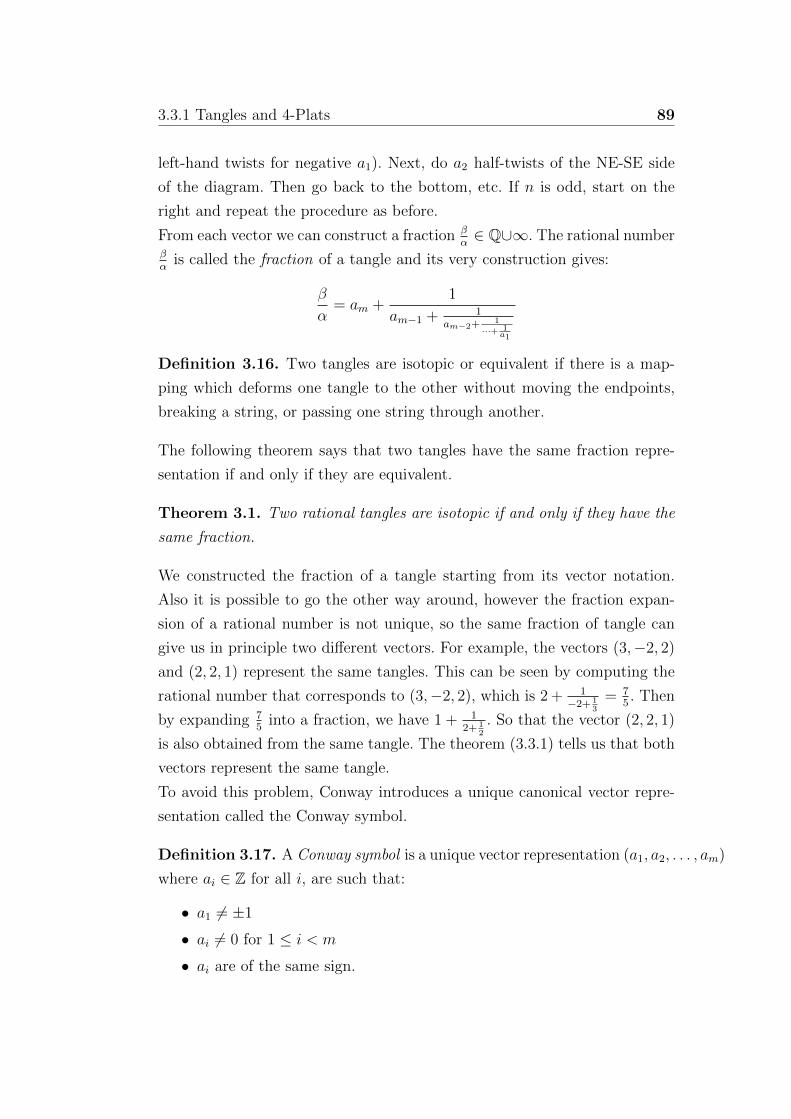
3.3.1 Tangles and 4-Plats 89

left-hand twists for negative a1). Next, do a2 half-twists of the NE-SE side

of the diagram. Then go back to the bottom, etc. If n is odd, start on the

right and repeat the procedure as before.

From each vector we can construct a fraction βα∈ Q∪∞. The rational number

βα

is called the fraction of a tangle and its very construction gives:

β

α= am +

1

am−1 + 1am−2+

1

···+ 1a1

Definition 3.16. Two tangles are isotopic or equivalent if there is a map-

ping which deforms one tangle to the other without moving the endpoints,

breaking a string, or passing one string through another.

The following theorem says that two tangles have the same fraction repre-

sentation if and only if they are equivalent.

Theorem 3.1. Two rational tangles are isotopic if and only if they have the

same fraction.

We constructed the fraction of a tangle starting from its vector notation.

Also it is possible to go the other way around, however the fraction expan-

sion of a rational number is not unique, so the same fraction of tangle can

give us in principle two different vectors. For example, the vectors (3,−2, 2)

and (2, 2, 1) represent the same tangles. This can be seen by computing the

rational number that corresponds to (3,−2, 2), which is 2 + 1−2+ 1

3

= 75. Then

by expanding 75

into a fraction, we have 1 + 12+ 1

2

. So that the vector (2, 2, 1)

is also obtained from the same tangle. The theorem (3.3.1) tells us that both

vectors represent the same tangle.

To avoid this problem, Conway introduces a unique canonical vector repre-

sentation called the Conway symbol.

Definition 3.17. A Conway symbol is a unique vector representation (a1, a2, . . . , am)

where ai ∈ Z for all i, are such that:

• a1 6= ±1

• ai 6= 0 for 1 ≤ i < m

• ai are of the same sign.

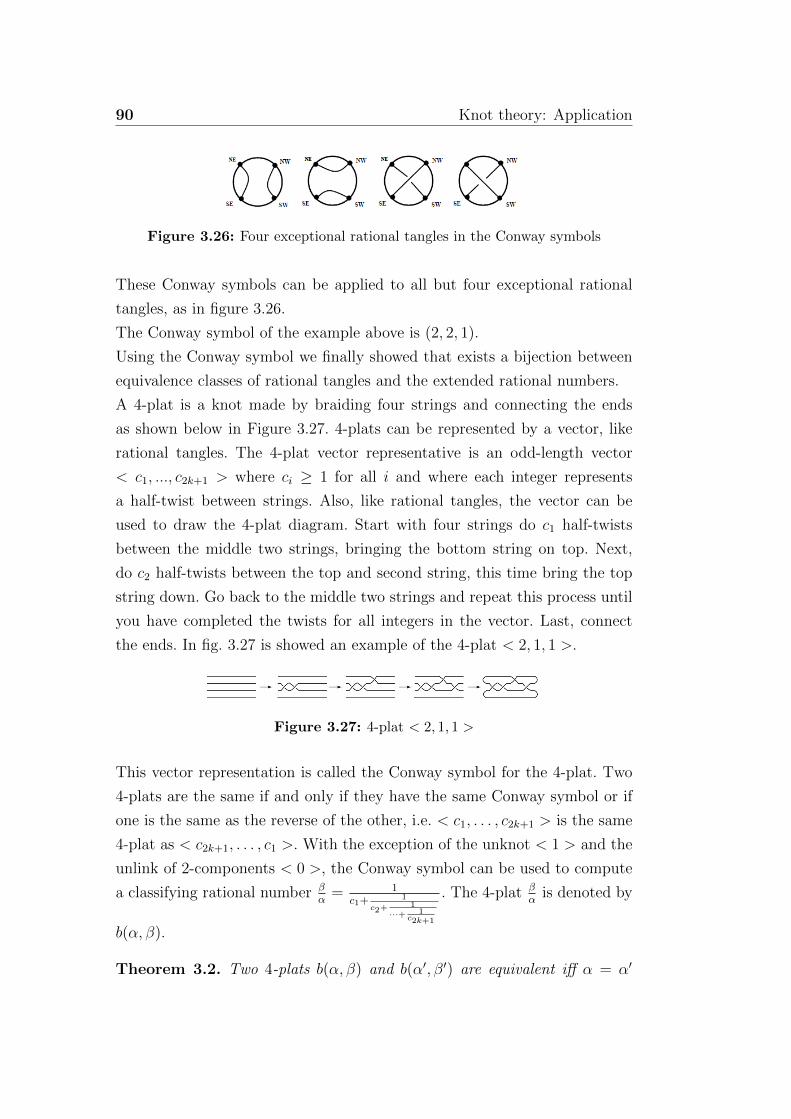
90 Knot theory: Application

Figure 3.26: Four exceptional rational tangles in the Conway symbols

These Conway symbols can be applied to all but four exceptional rational

tangles, as in figure 3.26.

The Conway symbol of the example above is (2, 2, 1).

Using the Conway symbol we finally showed that exists a bijection between

equivalence classes of rational tangles and the extended rational numbers.

A 4-plat is a knot made by braiding four strings and connecting the ends

as shown below in Figure 3.27. 4-plats can be represented by a vector, like

rational tangles. The 4-plat vector representative is an odd-length vector

< c1, ..., c2k+1 > where ci ≥ 1 for all i and where each integer represents

a half-twist between strings. Also, like rational tangles, the vector can be

used to draw the 4-plat diagram. Start with four strings do c1 half-twists

between the middle two strings, bringing the bottom string on top. Next,

do c2 half-twists between the top and second string, this time bring the top

string down. Go back to the middle two strings and repeat this process until

you have completed the twists for all integers in the vector. Last, connect

the ends. In fig. 3.27 is showed an example of the 4-plat < 2, 1, 1 >.

Figure 3.27: 4-plat < 2, 1, 1 >

This vector representation is called the Conway symbol for the 4-plat. Two

4-plats are the same if and only if they have the same Conway symbol or if

one is the same as the reverse of the other, i.e. < c1, . . . , c2k+1 > is the same

4-plat as < c2k+1, . . . , c1 >. With the exception of the unknot < 1 > and the

unlink of 2-components < 0 >, the Conway symbol can be used to compute

a classifying rational number βα

= 1c1+

1

c2+1

···+ 1c2k+1

. The 4-plat βα

is denoted by

b(α, β).

Theorem 3.2. Two 4-plats b(α, β) and b(α′, β′) are equivalent iff α = α′

3.3.2 The site-specific recombination 91

and β±1 ≡ β′(modα).

For example, let us look at the two 4-plats b(17, 5) and b(17, 7). The Conway

symbol corresponding to b(17, 5) is (3, 2, 2), and the Conway symbol corre-

sponding to b(17, 7) is (2, 2, 3). Therefore, these are equivalent 4-plats. Notice

17 = 17 and 5−1 ≡ 7(mod17).

Rational tangles and 4-plats are closely related by means of the rational num-

ber representation. Given a rational number βα

, if 0 < βα< 1, the denominator

of the rational tangle βα

gives the 4-plat b(α, β) and if βα≥ 1 the numerator

of the tangle βα

gives the 4-plat b(β,−α).

It follows the next theorem:

Theorem 3.3. Suppose the rational tangles with reduced fractions βα

andβ′

α′are given. If N(β

α) and N(β

′

α′) denote the corresponding rational knots

obtained by taking numerator of those tangles, then N(βα

) and N(β′

α′) are

topologically equivalent iff α = α′ and β±1 ≡ β′(modα).

3.2 The site-specific recombination

As discussed in the introduction of this section, DNA must be topologically

manipulated by enzymes in order for vital life processes to occur. One of these

enzymatic actions is called site-specific recombination. Site-specific recombi-

nation is a process by which a piece of DNA is moved to another position

on the molecule or to import a foreign piece of a DNA molecule into it. Re-

combination is used for gene rearrangement, gene regulation, copy number

control, and gene therapy. This process is mediated by an enzyme called a

recombinase. A small segment of the genetic sequence of the DNA that is

recognized by the recombinase is called a recombination site. A pair of sites

on the same molecule or different molecules, once recognized, are aligned and

then bound by the enzyme. This is the stage of the reaction called synapsis.

The DNA molecule and the enzyme itself are called the synaptic complexes.

Before recombination the DNA molecule is called the substrate and after re-

combination it is called the product. Once bound to the DNA, the enzyme

breaks the DNA at the two sites and then recombines the ends by exchanging

them. Each of the recombination sites is oriented by the order in which the

bases appear as one reads around the DNA strand in some predetermined

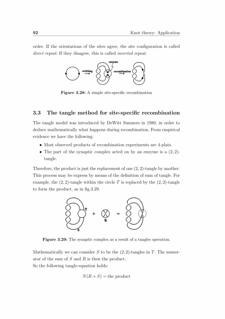
92 Knot theory: Application

order. If the orientations of the sites agree, the site configuration is called

direct repeat. If they disagree, this is called inverted repeat.

Figure 3.28: A simple site-specific recombination

3.3 The tangle method for site-specific recombination

The tangle model was introduced by DeWitt Sumners in 1980, in order to

deduce mathematically what happens during recombination. From empirical

evidence we have the following:

• Most observed products of recombination experiments are 4-plats.

• The part of the synaptic complex acted on by an enzyme is a (2, 2)-

tangle.

Therefore, the product is just the replacement of one (2, 2)-tangle by another.

This process may be express by means of the definition of sum of tangle. For

example, the (2, 2)-tangle within the circle T is replaced by the (2, 2)-tangle

to form the product, as in fig.3.29.

Figure 3.29: The synaptic complex as a result of a tangles operation.

Mathematically we can consider S to be the (2, 2)-tangles in T . The numer-

ator of the sum of S and R is then the product.

So the following tangle-equation holds:

N(R + S) = the product

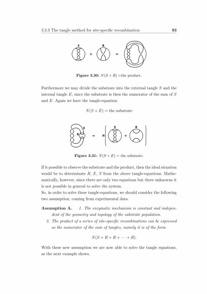
3.3.3 The tangle method for site-specific recombination 93

Figure 3.30: N(S +R) =the product.

Furthermore we may divide the substrate into the external tangle S and the

internal tangle E, since the substrate is then the numerator of the sum of S

and E. Again we have the tangle-equation:

N(S + E) = the substrate

Figure 3.31: N(S + E) = the substrate.

If it possible to observe the substrate and the product, then the ideal situation

would be to determinate R, E, S from the above tangle-equations. Mathe-

matically, however, since there are only two equations but three unknowns it

is not possible in general to solve the system.

So, in order to solve these tangle-equations, we should consider the following

two assumption, coming from experimental data.

Assumption A. 1. The enzymatic mechanism is constant and indepen-

dent of the geometry and topology of the substrate population.

2. The product of a series of site-specific recombinations can be expressed

as the numerator of the sum of tangles, namely it is of the form

N(S +R +R + · · ·+R).

With these new assumption we are now able to solve the tangle equations,

as the next example shows.

Bibliography

[1] E. F. Dorothy Buck. Applications of knot theory. 1984. Lecture notes

prepared for the American matematical society short course Application

of knot theory.

[2] M. Epple. Topology, matter, and space.

[3] M. Epple. Geometric aspects in the development of knot theory. History

of topology edition, 1999.

[4] L. Euler. Solutio problematis ad geometriam situs pertinentis. Com-

mentarii Academiae Scientiarum Imperialis Petropolitanae, 8:128–140,

1736.

[5] H.Helmholtz. Uber integrale der hydrodynamischen gleichungen, welche

den wirbelbewegungen entsprechen. English translation by P.G.Tait:

Philosophical Magazine, June 1867, 485-511.

[6] L. Kauffman. Knots. A short course in knot theory from Reidemeister

moves to state summations to Vassiliev Invariants and quantum fields.

[7] L. Kauffman. Knots and physics.

[8] K.Murasugi. Knot theory and its application. 1996.

[9] G. W. Leibniz. Addison-Wesley, 1 Abt:19–20, Math. Schriften.

[10] J. B. Listing. Vorstudien zur topologie.

[11] J. Maxwell. The scientific letters and papers of james clerk maxwell.

Edited and with a preface, note and introduction by P. M. Harman.

96 Bibliography

[12] K. Murasugi. Jones polynomials and classical conjectures in knot theory.

[13] C. Nash. Topology and Physics.

[14] P.G.Tait. On knots.

[15] R. H. F. Richard H. Crowell. Introduction knot theory. Springer-Verlag,

1977.

[16] P. Stackel. Gauss als Geometer, volume Xth Volume.

[17] W. Thomson. On vortex motion. See also Proceedings of the Royal

Society of Edinburgh, February 1867.

[18] H. Tietze. Uber die topologischen invarianten mehrdimensionaler man-

nigfaltigkeiten.

[19] V. Turaev. The yang-baxter equation and invariants of links.

[20] A. T. Vandermonde. Remarques sur les problemes de situation.

Acknowledgement

I owe my deepest gratitude to Prof. Rita Fioresi, my supervisor, whose guid-

ance, support and patience from the initial to the final level enable me to

write this dissertation. This thesis would not have been accomplished unless

her constant support and her professionalism, and I have to admit, I couldn’t

match up with it.

I am very grateful to Dr. Paola Sena, biologist at the University of Padova,

who had the courtesy to read the section about biology and who gave some

advice and to Dr. Alessia Cattabriga, who read my thesis in just one night.

I’m really thankful for the precious comments she made.

I also would like to make a special reference to Prof. Rama Mishra for her

suggestions and for the help with the research material.

I would like to thank my family and my friends for the support they provided

me.