Embed Size (px)
Citation preview
Knowledge Portal
BUSINESS ECONOMICS FOR CA FOUNDATION NOV 2018
By CA SANCHIT GROVER
CHAPTER 2:
THEORY OF DEMAND AND SUPPLY

About the AuthorCompleted his CA Course securing place in Top 6 All India Ranks - both at IPC and CPT level
Currently associated with Ernst & Young (one of the largest consultancy firms globally in the field of Tax Consultancy)
Wide range of experience in handling tax ralated matters (both direct tax and indirect tax)
for clients cutting across different sectors
Successfully handled GST Implementation projects for various Multi National Clients
Experience in handling issues related to UAE VAT and Australian GST
Speaker at various seminars on Taxation and Economics
What differentiates us from Others Discussion on Real Life Practical Issues with each Topic Use of tables and Flowcharts to summarize all Important Topics Interesting Learning techniques to grasp complexComplete Coverage of entire ICAI Question Bank includingRTPs and addtional questions on ICAI website Revisionary Video & Voice Clips for Last Day Preparations Last
CA SANCHIT GROVER(Senior tax consultant with Big 4 firm)

FOR FREE VIDEO LECTURES, SUMMARY NOTES FOLLOW YOUTUBE CHANNEL: CA knowledge portal Telegram channel: @foundation knowledge FOR LIVE FACE TO FACE & PEN DRIVE CLASSES CONTACT: AVJ Institute, Laxmi Nagar,Delhi.
(9310824912)
“Failure isn’t falling down, it’s refusing to get back up – Haarna Mana hai…!!” Page 1
Theory of Demand and Supply
This Chapter has been primarily divided into the following 3 units:-
Unit 1:- Theory of Consumer Behaviour
Unit 2:- Theory of Demand
Unit 3:- Theory of Supply
2.1:- Theory of Consumer Behaviour
What to Study in this Chapter
Concept of “Wants” in Economics
Meaning All desires, tastes and motives of human beings are called wants in Economics.
Wants may arise due to elementary and psychological causes.
Since the resources are limited, we have to choose between the urgent wants and the not so urgent
wants
Features of
‘Wants’
All wants of human beings exhibit some characteristic features:-
1) Wants are unlimited in number. They are never completely satisfied.
2) Wants differ in intensity. Some are urgent, others are felt less intensely.
3) Each want is satiable.
4) Wants are competitive. They compete each other for satisfaction because resources are scarce to
satisfy all wants.
5) Wants are complementary. Some wants can be satisfied only by using more than one good or
group of goods.
6) Wants are alternative.
7) Wants are subjective and relative.
8) Wants vary with time, place, and person.
9) Some wants recur again whereas others do not occur again and again.
10) Wants may become habits and customs.
11) Wants are affected by income, taste, fashion, advertisements and social customs.
12) Wants arise from multiple causes such as natural instincts, social obligation and individual’s
economic and social status
Classificati
on of
‘Wants’
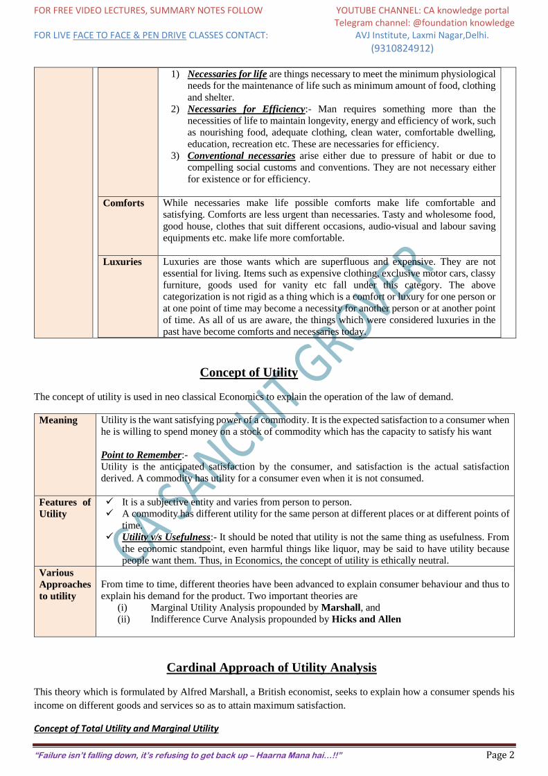
In Economics, wants are classified into three categories, viz., necessaries, comforts and luxuries.
Necessaries Necessaries are those which are essential for living. Necessaries are further sub-
divided into:- necessaries for life or existence, necessaries for efficiency and
conventional necessaries.
Concept of Utility
Law of Diminishing Marginal Utility
Concept of Consumer Surplus
Consumer Equilibrium as per Cardinal Approach
Consumer Equilibrium as per Ordinal Approach
FOR FREE VIDEO LECTURES, SUMMARY NOTES FOLLOW YOUTUBE CHANNEL: CA knowledge portal Telegram channel: @foundation knowledge FOR LIVE FACE TO FACE & PEN DRIVE CLASSES CONTACT: AVJ Institute, Laxmi Nagar,Delhi.
(9310824912)
“Failure isn’t falling down, it’s refusing to get back up – Haarna Mana hai…!!” Page 2
1) Necessaries for life are things necessary to meet the minimum physiological
needs for the maintenance of life such as minimum amount of food, clothing
and shelter.
2) Necessaries for Efficiency:- Man requires something more than the
necessities of life to maintain longevity, energy and efficiency of work, such
as nourishing food, adequate clothing, clean water, comfortable dwelling,
education, recreation etc. These are necessaries for efficiency.
3) Conventional necessaries arise either due to pressure of habit or due to
compelling social customs and conventions. They are not necessary either
for existence or for efficiency.
Comforts While necessaries make life possible comforts make life comfortable and
satisfying. Comforts are less urgent than necessaries. Tasty and wholesome food,
good house, clothes that suit different occasions, audio-visual and labour saving
equipments etc. make life more comfortable.
Luxuries Luxuries are those wants which are superfluous and expensive. They are not
essential for living. Items such as expensive clothing, exclusive motor cars, classy
furniture, goods used for vanity etc fall under this category. The above
categorization is not rigid as a thing which is a comfort or luxury for one person or
at one point of time may become a necessity for another person or at another point
of time. As all of us are aware, the things which were considered luxuries in the
past have become comforts and necessaries today.
Concept of Utility
The concept of utility is used in neo classical Economics to explain the operation of the law of demand.
Meaning Utility is the want satisfying power of a commodity. It is the expected satisfaction to a consumer when
he is willing to spend money on a stock of commodity which has the capacity to satisfy his want
Point to Remember:-
Utility is the anticipated satisfaction by the consumer, and satisfaction is the actual satisfaction
derived. A commodity has utility for a consumer even when it is not consumed.
Features of
Utility
It is a subjective entity and varies from person to person.
A commodity has different utility for the same person at different places or at different points of
time.
Utility v/s Usefulness:- It should be noted that utility is not the same thing as usefulness. From
the economic standpoint, even harmful things like liquor, may be said to have utility because
people want them. Thus, in Economics, the concept of utility is ethically neutral.
Various
Approaches
to utility
From time to time, different theories have been advanced to explain consumer behaviour and thus to
explain his demand for the product. Two important theories are
(i) Marginal Utility Analysis propounded by Marshall, and
(ii) Indifference Curve Analysis propounded by Hicks and Allen
Cardinal Approach of Utility Analysis
This theory which is formulated by Alfred Marshall, a British economist, seeks to explain how a consumer spends his
income on different goods and services so as to attain maximum satisfaction.
Concept of Total Utility and Marginal Utility
FOR FREE VIDEO LECTURES, SUMMARY NOTES FOLLOW YOUTUBE CHANNEL: CA knowledge portal Telegram channel: @foundation knowledge FOR LIVE FACE TO FACE & PEN DRIVE CLASSES CONTACT: AVJ Institute, Laxmi Nagar,Delhi.
(9310824912)
“Failure isn’t falling down, it’s refusing to get back up – Haarna Mana hai…!!” Page 3
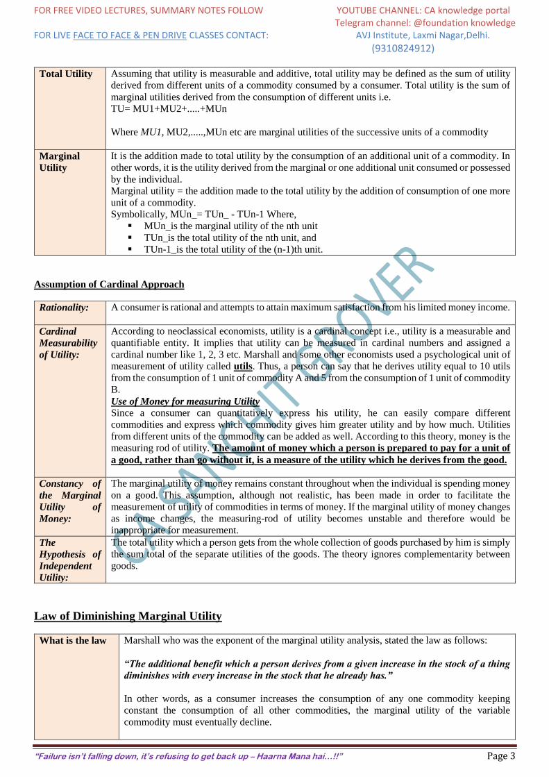
Total Utility Assuming that utility is measurable and additive, total utility may be defined as the sum of utility
derived from different units of a commodity consumed by a consumer. Total utility is the sum of
marginal utilities derived from the consumption of different units i.e.
TU= MU1+MU2+.....+MUn
Where MU1, MU2,.....,MUn etc are marginal utilities of the successive units of a commodity
Marginal
Utility
It is the addition made to total utility by the consumption of an additional unit of a commodity. In
other words, it is the utility derived from the marginal or one additional unit consumed or possessed
by the individual.
Marginal utility = the addition made to the total utility by the addition of consumption of one more
unit of a commodity.
Symbolically, MUn_= TUn_ - TUn-1 Where,
MUn_is the marginal utility of the nth unit
TUn_is the total utility of the nth unit, and
TUn-1_is the total utility of the (n-1)th unit.
Assumption of Cardinal Approach
Rationality: A consumer is rational and attempts to attain maximum satisfaction from his limited money income.
Cardinal
Measurability
of Utility:
According to neoclassical economists, utility is a cardinal concept i.e., utility is a measurable and
quantifiable entity. It implies that utility can be measured in cardinal numbers and assigned a
cardinal number like 1, 2, 3 etc. Marshall and some other economists used a psychological unit of
measurement of utility called utils. Thus, a person can say that he derives utility equal to 10 utils
from the consumption of 1 unit of commodity A and 5 from the consumption of 1 unit of commodity
B.
Use of Money for measuring Utility
Since a consumer can quantitatively express his utility, he can easily compare different
commodities and express which commodity gives him greater utility and by how much. Utilities
from different units of the commodity can be added as well. According to this theory, money is the
measuring rod of utility. The amount of money which a person is prepared to pay for a unit of
a good, rather than go without it, is a measure of the utility which he derives from the good.
Constancy of
the Marginal
Utility of
Money:
The marginal utility of money remains constant throughout when the individual is spending money
on a good. This assumption, although not realistic, has been made in order to facilitate the
measurement of utility of commodities in terms of money. If the marginal utility of money changes
as income changes, the measuring-rod of utility becomes unstable and therefore would be
inappropriate for measurement.
The
Hypothesis of
Independent
Utility:
The total utility which a person gets from the whole collection of goods purchased by him is simply
the sum total of the separate utilities of the goods. The theory ignores complementarity between
goods.
Law of Diminishing Marginal Utility
What is the law Marshall who was the exponent of the marginal utility analysis, stated the law as follows:
“The additional benefit which a person derives from a given increase in the stock of a thing
diminishes with every increase in the stock that he already has.”
In other words, as a consumer increases the consumption of any one commodity keeping
constant the consumption of all other commodities, the marginal utility of the variable
commodity must eventually decline.
FOR FREE VIDEO LECTURES, SUMMARY NOTES FOLLOW YOUTUBE CHANNEL: CA knowledge portal Telegram channel: @foundation knowledge FOR LIVE FACE TO FACE & PEN DRIVE CLASSES CONTACT: AVJ Institute, Laxmi Nagar,Delhi.
(9310824912)
“Failure isn’t falling down, it’s refusing to get back up – Haarna Mana hai…!!” Page 4
Remember:- It is the marginal utility and not the total utility which declines with the increase
in the consumption of a good.
Explanation of
law
The law of diminishing marginal utility is based on an important fact that while total wants of a
person are virtually unlimited, each single want is satiable i.e., each want is capable of being
satisfied. Since each want is satiable, as a consumer consumes more and more units of a good,
the intensity of his want for the good goes on decreasing and a point is reached where the
consumer no longer wants it. Thus, the greater the amount of a good a consumer has, the less
an additional unit is worth to him or her.
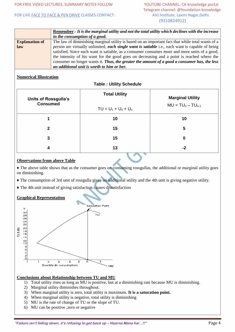
Numerical Illustration
Table : Utility Schedule
Units of Rossgulla’s Consumed
Total Utility
TU = U1 + U2 + Un
Marginal Utility
MU = TUn – TUn-1
1 10 10
2 15 5
3 15 0
4 13 -2
Observations from above Table
♦ The above table shows that as the consumer goes on consuming rossgullas, the additional or marginal utility goes
on diminishing.
♦ The consumption of 3rd unit of rossgulla gives no additional utility and the 4th unit is giving negative utility.
♦ The 4th unit instead of giving satisfaction causes dissatisfaction
Graphical Representation
Conclusions about Relationship between TU and MU
1) Total utility rises as long as MU is positive, but at a diminishing rate because MU is diminishing.
2) Marginal utility diminishes throughout.
3) When marginal utility is zero, total utility is maximum. It is a saturation point.
4) When marginal utility is negative, total utility is diminishing
5) MU is the rate of change of TU or the slope of TU.
6) MU can be positive ,zero or negative
FOR FREE VIDEO LECTURES, SUMMARY NOTES FOLLOW YOUTUBE CHANNEL: CA knowledge portal Telegram channel: @foundation knowledge FOR LIVE FACE TO FACE & PEN DRIVE CLASSES CONTACT: AVJ Institute, Laxmi Nagar,Delhi.
(9310824912)
“Failure isn’t falling down, it’s refusing to get back up – Haarna Mana hai…!!” Page 5
Are there any exceptions to this Law
In some cases a consumer gets increasing marginal utility with the increase in consumption.
Such cases are called as exception which are as follows-
1. Hobbies and Rare Collections: The law does not hold good in case of hobbies and rare collections like reading,
collection of stamps, coins, etc. Every additional unit gives more satisfaction i.e. the marginal utility tends to increase.
2. Abnormal Persons: The law does not apply to abnormal persons like misers, drunkards, musicians, drug addicts,
etc. who want more and more of the commodity they are in love with.
3. Indivisible Goods: The law cannot be applied in case of indivisible bulky goods like T. V. set, house, scooter, etc.
No one purchases more than one unit of such goods at a time.
Remember:- While this may be true in initial stages, beyond a certain limit these will also be subjected to diminishing
utility.
Concept of Consumer Equilibrium – Single product
A consumer tries to equalize marginal utility of a commodity with its price in order to maximize the satisfaction.
A consumer thus compares the price with the marginal utility of a commodity.
He keep on purchasing a commodity till MU > R In other words, so long as price is less, he buys more which
is also the basis of the law of demand.
The consumer is at equilibrium where:
Marginal Utility of the commodity = Price of the commodity
MUx = Px . MU money
MUX
Px = MU money
Impact of Change in Price of good on Consumer Equilibrium
The equality between marginal utility and price is disturbed when the price of the good falls.
1) What will happen in case price decreases
The consumer will consume more of the good so as to restore the equality between the marginal utility and price.
The marginal utility from the good will fall when he consumes more of the good. He will continue consuming
more till the marginal utility becomes equal to the new lower price.
2) What will happen in case price increases
When price of the good increases, he will buy less so as to equate the marginal utility to the higher price.
Conclusion
We can say that the downward sloping demand curve is directly derived from the marginal utility curve
Concept of Consumer Equilibrium – Two products
In reality, a consumer spends his money income to buy different commodities. In case of many commodities,
consumer equilibrium is explained with the Law of Equi-Marginal Utility.
The law states that a consumer will allocate his expenditure in a way that the utility gained from the last rupee
spent on each commodity is equal or the marginal utility each commodity is proportional to its price.
The consumer is said to be equilibrium when the following condition is met-
MUX
Px =
MUy
Py = MUmoney
OR
FOR FREE VIDEO LECTURES, SUMMARY NOTES FOLLOW YOUTUBE CHANNEL: CA knowledge portal Telegram channel: @foundation knowledge FOR LIVE FACE TO FACE & PEN DRIVE CLASSES CONTACT: AVJ Institute, Laxmi Nagar,Delhi.
(9310824912)
“Failure isn’t falling down, it’s refusing to get back up – Haarna Mana hai…!!” Page 6
MUX
MUy =
Px
Py
Notes
Assumptions/Limitations of this Law of Diminishing Marginal Utility
The law of diminishing marginal utility is applicable only under certain assumptions.
a) Homogenous units: The different units consumed should be identical in all respects. The habit, taste, temperament
and income of the consumer also should remain unchanged.
b) Standard units of Consumption: The different units consumed should consist of standard units. If a thirsty man
is given water by successive spoonfuls, the utility of the second spoonful of water may conceivably be greater than
the utility of the first.
c) Continuous Consumption: There should be no time gap or interval between the consumption of one unit and
another unit i.e. there should be continuous consumption.
d) The Law fails in the case of prestigious goods: The law may not apply to articles like gold, cash, diamonds etc.
where a greater quantity may increase the utility rather than diminish it. It also fails to apply in the case of hobbies,
alcohol, cigarettes, rare collections etc.
e) Case of related goods: Utility is not in fact independent. The shape of the utility curve may be affected by the
presence or absence of articles which are substitutes or complements. The utility obtained from tea may be seriously
affected if no sugar is available and the utility of bottled soft drinks will be affected by the availability of fresh
juice.
f) Based on unrealistic assumptions: The assumptions of cardinal measurability of utility, constancy of marginal
utility of money, continuous consumption and consumer rationality are unrealistic
Concept of Consumer Surplus
In our daily expenditure, we often find that the price we pay for a commodity is less than the satisfaction derived
from its consumption.
Therefore, we are ready to pay much higher price for a commodity than we actually have to pay.
E.g. Commodities like salt, newspaper, match box, etc. are very useful, but they are also very cheap.
From the purchase of such commodities we derive a good deal of extra satisfaction or surplus over and above the
price that we pay for them. This is consumer's surplus.
Marshall defined the concept of consumer’s surplus as the “excess of the price which a consumer would be willing to
pay rather than go without a thing over that which he actually does pay”, is called consumer’s surplus.”
Thus consumer’s surplus = what a consumer is ready to pay - what he actually pays
= Sum of Marginal Utilities - (Price × Units Purchased)
FOR FREE VIDEO LECTURES, SUMMARY NOTES FOLLOW YOUTUBE CHANNEL: CA knowledge portal Telegram channel: @foundation knowledge FOR LIVE FACE TO FACE & PEN DRIVE CLASSES CONTACT: AVJ Institute, Laxmi Nagar,Delhi.
(9310824912)
“Failure isn’t falling down, it’s refusing to get back up – Haarna Mana hai…!!” Page 7
= Total Utility - Total amount spent
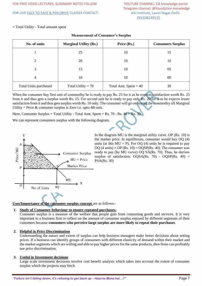
Measurement of Consumer’s Surplus
No. of units Marginal Utility (Rs.) Price (Rs.) Consumers Surplus
1 25 10 15
2 20 10 10
3 15 10 05
4 10 10 00
Total Units purchased Total Utility = 70 Total Amt. Spent = 40 30
When the consumer buy first unit of commodity he is ready to pay Rs. 25 for it as he expects satisfaction worth Rs. 25
from it and thus gets a surplus worth Rs. 15. For second unit he is ready to pay only Rs. 20 for it as he expects lesser
satisfaction from it and thus gets surplus worth Rs. 10 only. The consumer will go on buying the commodity till Marginal
Utility = Price & consumer surplus is Zero i.e. upto 4th unit.
Here, Consumer Surplus = Total Utility - Total Amt. Spent = Rs. 70 - Rs. 40 = Rs. 30.
We can represent consumers surplus with the following diagram.
In the diagram MU is the marginal utility curve. OP (Rs. 10) is
the market price. In equilibrium, consumer would buy OQ (4)
units (at this MU = P). For OQ (4) units he is required to pay
OQ (4 units) × OP (Rs. 10) = OQSP(Rs. 40). The consumer was
ready to pay (by MU curve) OQ SA(Rs. 70). Thus, he derives
surplus of satisfaction. OQSA(Rs. 70) - OQSP(Rs. 40) =
PSA(Rs. 30)
Uses/Importance of the consumer surplus concept are as follows:-
1. Study of Consumer behaviour to ensure repeated purchases:
Consumer surplus is a measure of the welfare that people gain from consuming goods and services. It is very
important to a business firm to reflect on the amount of consumer surplus enjoyed by different segments of their
customers because consumers who perceive large surplus are more likely to repeat their purchases.
2. Helpful in Price Discrimination
Understanding the nature and extent of surplus can help business managers make better decisions about setting
prices. If a business can identify groups of consumers with different elasticity of demand within their market and
the market segments which are willing and able to pay higher prices for the same products, then firms can profitably
use price discrimination.
3. Useful in Investment decisions
Large scale investment decisions involve cost benefit analysis which takes into account the extent of consumer
surplus which the projects may fetch.
FOR FREE VIDEO LECTURES, SUMMARY NOTES FOLLOW YOUTUBE CHANNEL: CA knowledge portal Telegram channel: @foundation knowledge FOR LIVE FACE TO FACE & PEN DRIVE CLASSES CONTACT: AVJ Institute, Laxmi Nagar,Delhi.
(9310824912)
“Failure isn’t falling down, it’s refusing to get back up – Haarna Mana hai…!!” Page 8
4. Useful in Pricing Decisions
Knowledge of consumer surplus is also important when a firm considers raising its product prices Customers who
enjoyed only a small amount of surplus may no longer be willing to buy products at higher prices. Firms making
such decisions should expect to make fewer sales if they increase prices.
5. Useful in deciding Taxation Policy
Consumer surplus usually acts as a guide to finance ministers when they decide on the products on which taxes
have to be imposed and the extent to which a commodity tax has to be raised. It is always desirable to impose taxes
or increase the rates of taxes on commodities yielding high consumer’s surplus because the loss of welfare to
citizens will be minimal
CRITICISMS of the consumer's surplus concept are as follows:-
1. Imaginary: The concept of consumer’s surplus is quite imaginary idea. One has to imagine what you are prepared
to pay and you proceed to deduct from that what you actually pay. It is all hypothetical and unreal.
2. Cardinal measurement is not possible: Consumer’s surplus cannot be measured precisely because it is difficult to
measure the total utilities and marginal utilities of the commodities consumed in quantitative terms.
3. Ignores the interdependence between goods: The concept of consumer’s surplus does not consider the effect of
availability and non-availability of substitutes and complementary goods on the consumption of a particular commodity.
Actually consumer surplus derived from a commodity is affected by substitutes and complementary goods.
4. Cannot be measured in terms of money: This is because the marginal utility of money changes as purchases are
made and the consumer's stock of money diminishes. But, Marshall assumed that the marginal utility of money to be
constant.
5. Not applicable to Necessaries: It does not apply to the necessaries of life. In such cases the surplus is immeasurable
e.g. - Food and Water. Consumer surplus is infinite because a consumer will stake whole of his income rather than go
without them.
6. Not applicable to prestige: e.g. - Diamonds jewellery, etc. fall in their prices lead to a fall in consumer's surplus.
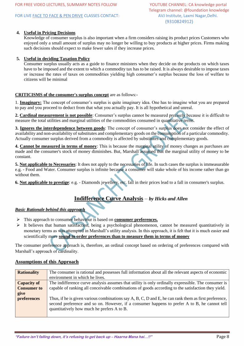
Indifference Curve Analysis – by Hicks and Allen
Basic Rationale behind this approach
This approach to consumer behaviour is based on consumer preferences.
It believes that human satisfaction, being a psychological phenomenon, cannot be measured quantitatively in
monetary terms as was attempted in Marshall’s utility analysis. In this approach, it is felt that it is much easier and
scientifically more sound to order preferences than to measure them in terms of money
The consumer preference approach is, therefore, an ordinal concept based on ordering of preferences compared with
Marshall’s approach of cardinality.
Assumptions of this Approach
Rationality The consumer is rational and possesses full information about all the relevant aspects of economic
environment in which he lives. Capacity of
Consumer to
give
preferences
The indifference curve analysis assumes that utility is only ordinally expressible. The consumer is
capable of ranking all conceivable combinations of goods according to the satisfaction they yield.
Thus, if he is given various combinations say A, B, C, D and E, he can rank them as first preference,
second preference and so on. However, if a consumer happens to prefer A to B, he cannot tell
quantitatively how much he prefers A to B.
FOR FREE VIDEO LECTURES, SUMMARY NOTES FOLLOW YOUTUBE CHANNEL: CA knowledge portal Telegram channel: @foundation knowledge FOR LIVE FACE TO FACE & PEN DRIVE CLASSES CONTACT: AVJ Institute, Laxmi Nagar,Delhi.
(9310824912)
“Failure isn’t falling down, it’s refusing to get back up – Haarna Mana hai…!!” Page 9
Transitive Consumer’s choices are assumed to be transitive. If the consumer prefers combination A to B, and
B to C, then he must prefer combination A to C. In other words, he has a consistent consumption
pattern Law of
monotonic
Consumer
Preference
If combination A has more commodities than combination B, then A must be preferred to B.
Concept of Indifference Curve
An indifference curve is a curve which represents all those combinations of two goods which give same
satisfaction to the consumer.
Since all the combinations on an indifference curve give equal satisfaction to the consumer, the consumer is
indifferent among them. In other words, since all the combinations provide the same level of satisfaction the
consumer prefers them equally and does not mind which combination he gets.
An Indifference curve is also called iso- utility curve or equal utility curve.
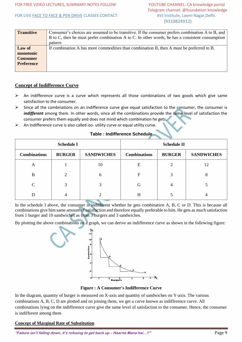
Table : Indifference Schedule
Schedule I Schedule II
Combinations BURGER SANDWICHES Combinations BURGER SANDWICHES
A 1 10 E 2 12
B 2 6 F 3 8
C 3 3 G 4 5
D 4 2 H 5 4
In the schedule I above, the consumer is indifferent whether he gets combination A, B, C or D. This is because all
combinations give him same amount of satisfaction and therefore equally preferable to him. He gets as much satisfaction
from 1 burger and 10 sandwiches as from 3 burgers and 3 sandwiches.
By plotting the above combinations on a graph, we can derive an indifference curve as shown in the following figure:
Figure : A Consumer's Indifference Curve
In the diagram, quantity of burger is measured on X-axis and quantity of sandwiches on Y-axis. The various
combinations A, B, C, D are plotted and on joining them, we get a curve known as indifference curve. All
combinations lying on the indifference curve give the same level of satisfaction to the consumer. Hence, the consumer
is indifferent among them
Concept of Marginal Rate of Substitution
FOR FREE VIDEO LECTURES, SUMMARY NOTES FOLLOW YOUTUBE CHANNEL: CA knowledge portal Telegram channel: @foundation knowledge FOR LIVE FACE TO FACE & PEN DRIVE CLASSES CONTACT: AVJ Institute, Laxmi Nagar,Delhi.
(9310824912)
“Failure isn’t falling down, it’s refusing to get back up – Haarna Mana hai…!!” Page 10
Marginal Rate of Substitution (MRS) is the rate at which a consumer is prepared to exchange goods X and Y.
We can define MRS of X for Y as the amount of Y whose loss can just be compensated by a unit gain of X in such a
manner that the level of satisfaction remains the same.
The marginal rate of substitution of X for Y (MRSxy) is equal to MUx/ MUy
We notice that MRS is falling i.e., as the consumer has more and more units of Burger, he is prepared to give up less
and less units of Sandwiches. There are two reasons for this.
1. The want for a particular good is satiable so that when a consumer has more of it, his intensity of want for it
decreases. Thus, in our example, when the consumer has more units of food, his intensity of desire for additional
units of food decreases.
2. Most goods are imperfect substitutes of one another. MRS would remain constant if they could substitute one
another perfectly
Properties of Indifference Curve
(i) Indifference curves slope downward to the right – Reason : Law of Monotonic Consumer Preference
This property implies that the two commodities can be substituted for each other and when the amount of one
good in the combination is increased, the amount of the other good is reduced. This is essential if the level of
satisfaction is to remain the same on an indifference curve.
Exam points
(ii) Indifference curves are always convex to the origin: Reason: Diminishing MRS
It has been observed that as more and more of one commodity (X) is substituted for another (Y), the consumer is
willing to part with less and less of the commodity being substituted (i.e. Y). This is called diminishing marginal
rate of substitution. Thus, in our example of burger and sandwich, as a consumer has more and more units of
burger, he is prepared to forego less and less units of sandwich. This happens mainly because the want for a
particular good is satiable and as a person has more and more of a good, his intensity of want for that good goes
on diminishing. In other words, the subjective value attached to the additional quantity of a commodity decreases
fast in relation to the other commodity whose total quantity is decreasing. This diminishing marginal rate of
substitution gives convex shape to the indifference curves.
Two Extreme Situations
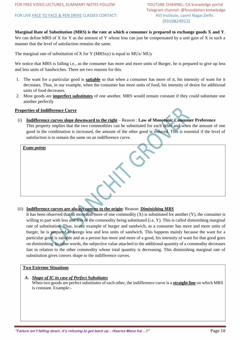
A. Shape of IC in case of Perfect Substitutes
When two goods are perfect substitutes of each other, the indifference curve is a straight line on which MRS
is constant. Example:-
FOR FREE VIDEO LECTURES, SUMMARY NOTES FOLLOW YOUTUBE CHANNEL: CA knowledge portal Telegram channel: @foundation knowledge FOR LIVE FACE TO FACE & PEN DRIVE CLASSES CONTACT: AVJ Institute, Laxmi Nagar,Delhi.
(9310824912)
“Failure isn’t falling down, it’s refusing to get back up – Haarna Mana hai…!!” Page 11
B. Shape of IC in case of Perfect Complementary Goods
When two goods are perfect complementary goods the indifference curve will consist of two straight lines
with a right angle bent which is convex to the origin, or in other words, it will be L shaped.
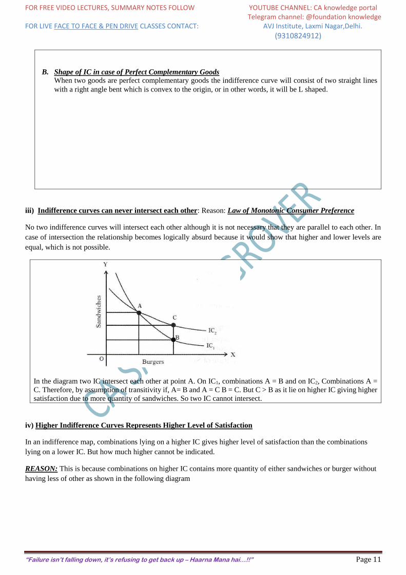
iii) Indifference curves can never intersect each other: Reason: Law of Monotonic Consumer Preference
No two indifference curves will intersect each other although it is not necessary that they are parallel to each other. In
case of intersection the relationship becomes logically absurd because it would show that higher and lower levels are
equal, which is not possible.
In the diagram two IC intersect each other at point A. On IC1, combinations A = B and on IC2, Combinations A =
C. Therefore, by assumption of transitivity if, A= B and A = C B = C. But C > B as it lie on higher IC giving higher
satisfaction due to more quantity of sandwiches. So two IC cannot intersect.
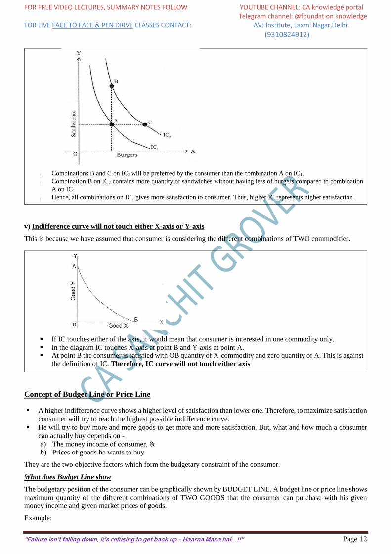
iv) Higher Indifference Curves Represents Higher Level of Satisfaction
In an indifference map, combinations lying on a higher IC gives higher level of satisfaction than the combinations
lying on a lower IC. But how much higher cannot be indicated.
REASON: This is because combinations on higher IC contains more quantity of either sandwiches or burger without
having less of other as shown in the following diagram
FOR FREE VIDEO LECTURES, SUMMARY NOTES FOLLOW YOUTUBE CHANNEL: CA knowledge portal Telegram channel: @foundation knowledge FOR LIVE FACE TO FACE & PEN DRIVE CLASSES CONTACT: AVJ Institute, Laxmi Nagar,Delhi.
(9310824912)
“Failure isn’t falling down, it’s refusing to get back up – Haarna Mana hai…!!” Page 12
Combinations B and C on IC2 will be preferred by the consumer than the combination A on IC1. Combination B on IC2 contains more quantity of sandwiches without having less of burgers compared to combination
A on IC1
Hence, all combinations on IC2 gives more satisfaction to consumer. Thus, higher IC represents higher satisfaction
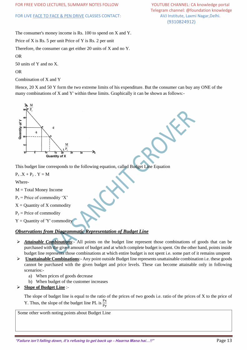
v) Indifference curve will not touch either X-axis or Y-axis
This is because we have assumed that consumer is considering the different combinations of TWO commodities.
If IC touches either of the axis, it would mean that consumer is interested in one commodity only.
In the diagram IC touches X-axis at point B and Y-axis at point A.
At point B the consumer is satisfied with OB quantity of X-commodity and zero quantity of A. This is against
the definition of IC. Therefore, IC curve will not touch either axis
Concept of Budget Line or Price Line
A higher indifference curve shows a higher level of satisfaction than lower one. Therefore, to maximize satisfaction
consumer will try to reach the highest possible indifference curve.
He will try to buy more and more goods to get more and more satisfaction. But, what and how much a consumer
can actually buy depends on -
a) The money income of consumer, &
b) Prices of goods he wants to buy.
They are the two objective factors which form the budgetary constraint of the consumer.
What does Budget Line show
The budgetary position of the consumer can be graphically shown by BUDGET LINE. A budget line or price line shows
maximum quantity of the different combinations of TWO GOODS that the consumer can purchase with his given
money income and given market prices of goods.
Example:
FOR FREE VIDEO LECTURES, SUMMARY NOTES FOLLOW YOUTUBE CHANNEL: CA knowledge portal Telegram channel: @foundation knowledge FOR LIVE FACE TO FACE & PEN DRIVE CLASSES CONTACT: AVJ Institute, Laxmi Nagar,Delhi.
(9310824912)
“Failure isn’t falling down, it’s refusing to get back up – Haarna Mana hai…!!” Page 13
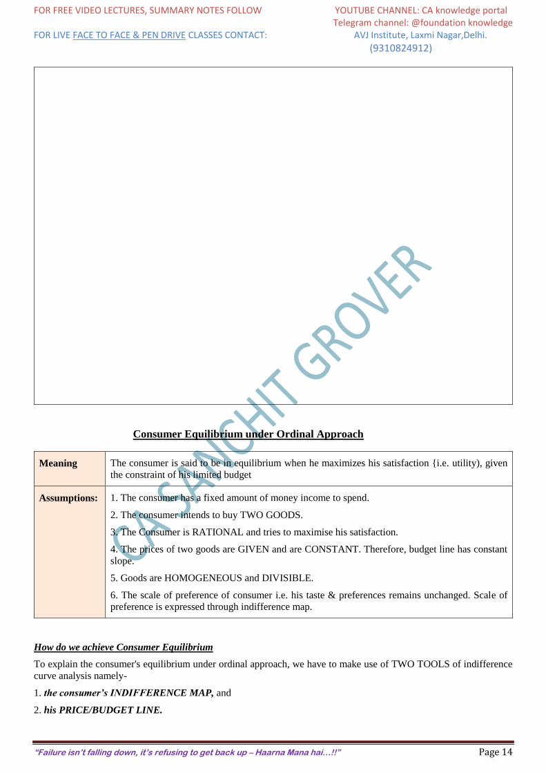
The consumer's money income is Rs. 100 to spend on X and Y.
Price of X is Rs. 5 per unit Price of Y is Rs. 2 per unit
Therefore, the consumer can get either 20 units of X and no Y.
OR
50 units of Y and no X.
OR
Combination of X and Y
Hence, 20 X and 50 Y form the two extreme limits of his expenditure. But the consumer can buy any ONE of the
many combinations of X and Y' within these limits. Graphically it can be shown as follows:-
This budget line corresponds to the following equation, called Budget Line Equation
Px .X + Py . Y = M
Where-
M = Total Money Income
Px = Price of commodity ‘X’
X = Quantity of X commodity
Py = Price of commodity
Y = Quantity of 'Y' commodity
Observations from Diagrammatic Representation of Budget Line
Attainable Combinations:- All points on the budget line represent those combinations of goods that can be
purchased with the given amount of budget and at which complete budget is spent. On the other hand, points inside
budget line represents those combinations at which entire budget is not spent i.e. some part of it remains unspent
Unattainable Combinations:- Any point outside Budget line represents unattainable combination i.e. these goods
cannot be purchased with the given budget and price levels. These can become attainable only in following
scenarios:-
a) When prices of goods decrease
b) When budget of the customer increases
Slope of Budget Line :-
The slope of budget line is equal to the ratio of the prices of two goods i.e. ratio of the prices of X to the price of
Y. Thus, the slope of the budget line PL is Px
Py
Some other worth noting points about Budget Line
FOR FREE VIDEO LECTURES, SUMMARY NOTES FOLLOW YOUTUBE CHANNEL: CA knowledge portal Telegram channel: @foundation knowledge FOR LIVE FACE TO FACE & PEN DRIVE CLASSES CONTACT: AVJ Institute, Laxmi Nagar,Delhi.
(9310824912)
“Failure isn’t falling down, it’s refusing to get back up – Haarna Mana hai…!!” Page 14
Consumer Equilibrium under Ordinal Approach
Meaning The consumer is said to be in equilibrium when he maximizes his satisfaction {i.e. utility), given
the constraint of his limited budget
Assumptions:
1. The consumer has a fixed amount of money income to spend.
2. The consumer intends to buy TWO GOODS.
3. The Consumer is RATIONAL and tries to maximise his satisfaction.
4. The prices of two goods are GIVEN and are CONSTANT. Therefore, budget line has constant
slope.
5. Goods are HOMOGENEOUS and DIVISIBLE.
6. The scale of preference of consumer i.e. his taste & preferences remains unchanged. Scale of
preference is expressed through indifference map.
How do we achieve Consumer Equilibrium
To explain the consumer's equilibrium under ordinal approach, we have to make use of TWO TOOLS of indifference
curve analysis namely-
1. the consumer’s INDIFFERENCE MAP, and
2. his PRICE/BUDGET LINE.
FOR FREE VIDEO LECTURES, SUMMARY NOTES FOLLOW YOUTUBE CHANNEL: CA knowledge portal Telegram channel: @foundation knowledge FOR LIVE FACE TO FACE & PEN DRIVE CLASSES CONTACT: AVJ Institute, Laxmi Nagar,Delhi.
(9310824912)
“Failure isn’t falling down, it’s refusing to get back up – Haarna Mana hai…!!” Page 15
The CONSUMER’S INDIFFERENCE MAP shows all indifference curves which rank the consumer's preferences
between various possible combinations of TWO commodities.
To maximises his satisfaction consumer would like to reach highest possible indifference curve.
The slope of IC at any one point shows the MARGINAL RATE OF SUBSTITUTION (which diminishes).
Thus, MRSxy = MUX
MUy
To maximise satisfaction consumer will try to reach the highest possible IC and so will try to buy more and more
of the two commodities.
But there are limits to which he can go on and on.
♦ These limits are imposed (i) his money income, & (ii) prices of the commodities. These limits are described by
PRICE/BUDGET LINE which shows the various combinations of two commodities the consumer can afford to buy.
♦ All the combinations lying on the budget line are affordable by the consumer. Any, combination lying beyond budget
line is unaffordable.
♦ The slope of budget/price line shows the ratio of the prices of two commodities i.e. Px
Py
♦ Now we can show how a consumer reaches equilibrium i.e., how he allocates his money expenditure between
commodities X and Y and gets maximum satisfaction.
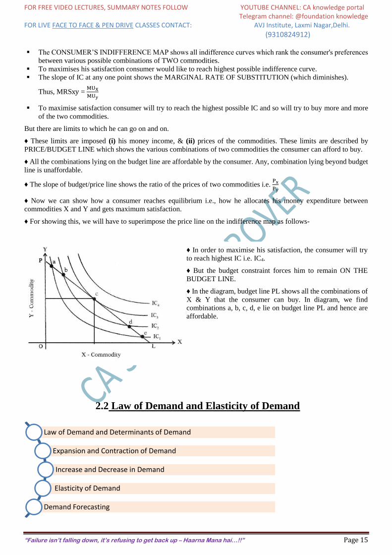
♦ For showing this, we will have to superimpose the price line on the indifference map as follows-
♦ In order to maximise his satisfaction, the consumer will try
to reach highest IC i.e. IC4.
♦ But the budget constraint forces him to remain ON THE
BUDGET LINE.
♦ In the diagram, budget line PL shows all the combinations of
X & Y that the consumer can buy. In diagram, we find
combinations a, b, c, d, e lie on budget line PL and hence are
affordable.
2.2 Law of Demand and Elasticity of Demand
Law of Demand and Determinants of Demand
Expansion and Contraction of Demand
Increase and Decrease in Demand
Elasticity of Demand
Demand Forecasting
FOR FREE VIDEO LECTURES, SUMMARY NOTES FOLLOW YOUTUBE CHANNEL: CA knowledge portal Telegram channel: @foundation knowledge FOR LIVE FACE TO FACE & PEN DRIVE CLASSES CONTACT: AVJ Institute, Laxmi Nagar,Delhi.
(9310824912)
“Failure isn’t falling down, it’s refusing to get back up – Haarna Mana hai…!!” Page 16
The market system is governed by market mechanism. In a market system, the price of a commodity or service is
determined by the forces of demand and supply. While buyers constitute the demand side of the market, sellers make
the supply side of that market
Meaning of Demand
Initial
Concept
The concept ‘demand’ refers to the quantity of a good or service that consumers are willing and able
to purchase at various prices during a given period of time
Demand v/s
Desire
It is to be noted that demand, in Economics, is something more than the desire to purchase, though
desire is one element of it. A beggar, for instance, may desire food, but due to lack of means to
purchase it, his demand is not effective.
Thus, effective demand for a thing depends on
(i) desire
(ii) means to purchase and
(iii) willingness to use those means for that purchase.
Unless desire is backed by purchasing power or ability to pay, and willingness to pay, it does not
constitute demand.
Remember:- It is only the Effective demand alone which would figure in economic analysis and
business decisions.
Points to be
noted about
quantity
demanded
Two things are to be noted about the quantity demanded:-
The quantity demanded is always expressed at a given price. At different prices, different quantities
of a commodity are generally demanded.
The quantity demanded is a flow. We are concerned not with a single isolated purchase, but with a
continuous flow of purchases and we must therefore express demand as ‘so much per period of time’
i.e., one thousand dozens of oranges per day, seven thousand dozens of oranges per week and so on
Final
Definition of
Demand
“By demand, we mean the various quantities of a given commodity or service which consumers
would buy in one market during a given period of time, at various prices, or at various incomes,
or at various prices of related goods”.
Determinants of Demand
Price of the
commodity:
Ceteris paribus i.e. other things being equal, the demand for a commodity is inversely related to
its price. It implies that a rise in the price of a commodity brings about a fall in the quantity
purchased and vice-versa. This happens because of income and substitution effects – discussed in
detail later on in the Chapter
Price of related
commodities:
Related commodities are of two types: (a) complementary goods and (ii) competing goods or
substitutes.
Complementary goods
These are those goods which are consumed together or simultaneously. For example; tea and
sugar, automobile and petrol and pen and ink. When two commodities are complements, a fall in
the price of one (other things being equal) will cause the demand for the other to rise. For example,
a fall in the price of petrol-driven cars would lead to a rise in the demand for petrol. Similarly, a
fall in the price of fountain pens will cause a rise in the demand for ink. The reverse will be the
case when the price of a complement rises.
Conclusion:- Thus, there is an inverse relation between the demand for a good and the price of
its complement.
Substitute Goods
FOR FREE VIDEO LECTURES, SUMMARY NOTES FOLLOW YOUTUBE CHANNEL: CA knowledge portal Telegram channel: @foundation knowledge FOR LIVE FACE TO FACE & PEN DRIVE CLASSES CONTACT: AVJ Institute, Laxmi Nagar,Delhi.
(9310824912)
“Failure isn’t falling down, it’s refusing to get back up – Haarna Mana hai…!!” Page 17
Two commodities are called competing goods or substitutes when they satisfy the same want and
can be used with ease in place of one another. For example, tea and coffee, ink pen and ball pen,
are substitutes for each other and can be used in place of one another easily. When goods are
substitutes, a fall in the price of one (ceteris paribus) leads to a fall in the quantity demanded of
its substitutes. For example, if the price of tea falls, people will try to substitute it for coffee and
demand more of it and less of coffee i.e. the demand for tea will rise and that of coffee will fall.
Conclusion:- There is direct or positive relation between the demand for a product and the
price of its substitutes
Income of the
consumer:
Other things being equal, the demand for a commodity depends upon the money income of the
consumer. The purchasing power of the consumer is determined by the level of his income.
Normal Goods
In most cases, the larger the average money income of the consumer, the larger is the quantity
demanded of a particular good. The nature of relationship between income and quantity demanded
depends upon the nature of consumer goods. Most of the consumption goods fall under the
category of normal goods. These are demanded in increasing quantities as consumers’ income
increases. Household furniture, clothing, automobiles, consumer durables and semi durables etc.
fall in this category.
Essential consumer goods such as food grains, fuel, cooking oil, necessary clothing etc., satisfy
the basic necessities of life and are consumed by all individuals in a society. A change in
consumers’ income, although will cause an increase in demand for these necessities, but this
increase will be less than proportionate to the increase in income. This is because as people
become richer, there is a relative decline in the importance of food and other non durable goods
FOR FREE VIDEO LECTURES, SUMMARY NOTES FOLLOW YOUTUBE CHANNEL: CA knowledge portal Telegram channel: @foundation knowledge FOR LIVE FACE TO FACE & PEN DRIVE CLASSES CONTACT: AVJ Institute, Laxmi Nagar,Delhi.
(9310824912)
“Failure isn’t falling down, it’s refusing to get back up – Haarna Mana hai…!!” Page 18
in the overall consumption basket and a rise in the importance of durable goods such as a TV, car,
house etc.
Inferior Goods
There are some commodities for which the quantity demanded rises only up to a certain level of
income and decreases with an increase in money income beyond this level. These goods are called
inferior goods.
How to differentiate between normal goods and inferior goods
A same good may be normal for one condition and may be inferior in another. For example Bajra
may become an inferior good for a person when his income increases above a certain level and
he can now afford better substitutes such as wheat. Demand for luxury goods and prestige goods
arise beyond a certain level of consumers’ income and keep rising as income increases.
How is this factor relevant for decision making
Business managers should be fully aware of the nature of goods which they produce (or the nature
of need which their products satisfy) and the nature of relationship of quantities demanded with
changes in consumer incomes. For assessing the current as well as future demand for their
products, they should also recognize the movements in the macro economic variables that a_ect
the incomes of the consumers
Tastes and
preferences of
consumers:
The demand for a commodity also depends upon the tastes and preferences of consumers and
changes in them over a period of time. Goods which are modern or more in fashion command
higher demand than goods which are of old design and out of fashion. Consumers may perceive
a product as obsolete and discard it before it is fully utilised and prefer another good which is
currently in fashion. For example, there is greater demand for LCD/LED televisions and more
and more people are discarding their ordinary television sets even though they could have used it
for some more years.
‘Demonstration effect’ or ‘bandwagon effect’:- It plays an important role in determining the
demand for a product. An individual’s demand for LCD/LED television may be affected by his
seeing one in his neighbour’s or friend’s house, either because he likes what he sees or because
he figures out that if his neighbour or friend can afford it, he too can. A person may develop a
taste or preference for wine after tasting some, but he may also develop it after discovering that
serving it enhances his prestige.
Snob Effect or Veblen Effect
On the contrary, when a product becomes common among all, some people decrease or altogether
stop its consumption. This is called ‘snob effect’. Highly priced goods are consumed by status
seeking rich people to satisfy their need for conspicuous consumption. This is called ‘Veblen
effect’ (named after the American economist Thorstein Veblen). In any case, people have tastes
and preferences and these change, sometimes, due to external and sometimes, due to internal
causes and influence demand.
Consumers’
Expectations:
Consumers’ expectations regarding future prices, income, supply conditions etc. in_uence current
demand. If the consumers expect increase in future prices, increase in income and shortages in
supply, more quantities will be demanded. If they expect a fall in price, they will postpone their
purchases of nonessential commodities and therefore, the current demand for them will fall
Other Factors
Size of
population:
Generally, larger the size of population of a country or a region, greater is the demand for
commodities in general
FOR FREE VIDEO LECTURES, SUMMARY NOTES FOLLOW YOUTUBE CHANNEL: CA knowledge portal Telegram channel: @foundation knowledge FOR LIVE FACE TO FACE & PEN DRIVE CLASSES CONTACT: AVJ Institute, Laxmi Nagar,Delhi.
(9310824912)
“Failure isn’t falling down, it’s refusing to get back up – Haarna Mana hai…!!” Page 19
Composition of
population
If there are more old people in a region, the demand for spectacles, walking sticks, etc. will be
high. Similarly, if the population consists of more of children, demand for toys, baby foods,
toffees, etc. will be more
The level of
National
Income and its
Distribution
The level of national income is a crucial determinant of market demand. Higher the national
income, higher will be the demand for all normal goods and services.
The wealth of a country may be unevenly distributed so that there are a few very rich people while
the majority are very poor. Under such conditions, the propensity to consume of the country will
be relatively less, because the propensity to consume of the rich people is less than that of the
poor people. Consequently, the demand for consumer goods will be comparatively less. If the
distribution of income is more equal, then the propensity to consume of the country as a whole
will be relatively high indicating higher demand for goods.
Consumer-
credit facility
and interest
rates:
Availability of credit facilities induces people to purchase more than what their current incomes
permit them. Credit facilities mostly determine the demand for durable goods which are expensive
and require bulk payments at the time of purchase. Low rates of interest encourage people to
borrow and therefore demand will be more. Apart from above, factors such as government policy
in respect of taxes and subsidies, business conditions, wealth, socioeconomic class, group, level
of education, marital status, weather conditions, salesmanship and advertisements, habits,
customs and conventions also play an important role in influencing demand
Demand Function
The demand function states the relationship between the demand for a product (the dependent variable) and its
determinants (the independent or explanatory variables). A demand function may be expressed as follows:
Dx = f (PX, M, PY, PC, T, A)
Where Dx is the quantity demanded of product X
PX is the price of the commodity
M is the money income of the consumer
PY is the price of its substitutes
PC is the price of its complementary goods
T is consumer tastes, and preferences
A is advertisement expenditure
Law of Demand
According to the law of demand, other things being equal, if the price of a commodity falls, the quantity
demanded of it will rise and if the price of a commodity rises, its quantity demanded will decline. Thus, there is
an inverse relationship between price and quantity demanded, ceteris paribus
Definition of the Law of Demand
Prof. Alfred Marshall defined the Law thus: “The greater the amount to be sold, the smaller must be the price at
which it is offered in order that it may find purchasers or in other words the amount demanded increases with a fall
in price and diminishes with a rise in price”.
FOR FREE VIDEO LECTURES, SUMMARY NOTES FOLLOW YOUTUBE CHANNEL: CA knowledge portal Telegram channel: @foundation knowledge FOR LIVE FACE TO FACE & PEN DRIVE CLASSES CONTACT: AVJ Institute, Laxmi Nagar,Delhi.
(9310824912)
“Failure isn’t falling down, it’s refusing to get back up – Haarna Mana hai…!!” Page 20
Demand Schedule
A demand schedule is a table which presents the different prices of a good and the corresponding quantity
demanded per unit of time.
A demand schedule is drawn upon the assumption that all the other influences remain unchanged. It thus attempts
to isolate the influence exerted by the price of the good upon the amount sold.
Demand schedule and curve may be two types:
(A) Individual demand schedule: It shows the quantity of the commodities that one consumer will buy at selected
prices.
Price of sugar Rs. per kg. Quantity Demanded kgs. per month
1 5
2 4
3 3
4 2
5 1
(B) Market demand schedule: It is a table showing different quantities of a commodity that ALL THE CONSUMERS
are willing to buy at different prices, during a given period of time When we add the individual demands for various
schedules we get market demand schedule.
Price of sugar Rs. per kg. Quantity Demanded p.m. kgs.
Market Demand A + B
Consumer A Consumer B
1 5 6 5 + 6=11
2 4 5 4 + 5 = 9
3 3 4 3 + 4 = 7
4 2 3 2 + 3 = 5
5 1 2 1+2 = 3
It indicates that both individual demand and market demand have inverse relationship between price and quantity
demanded.
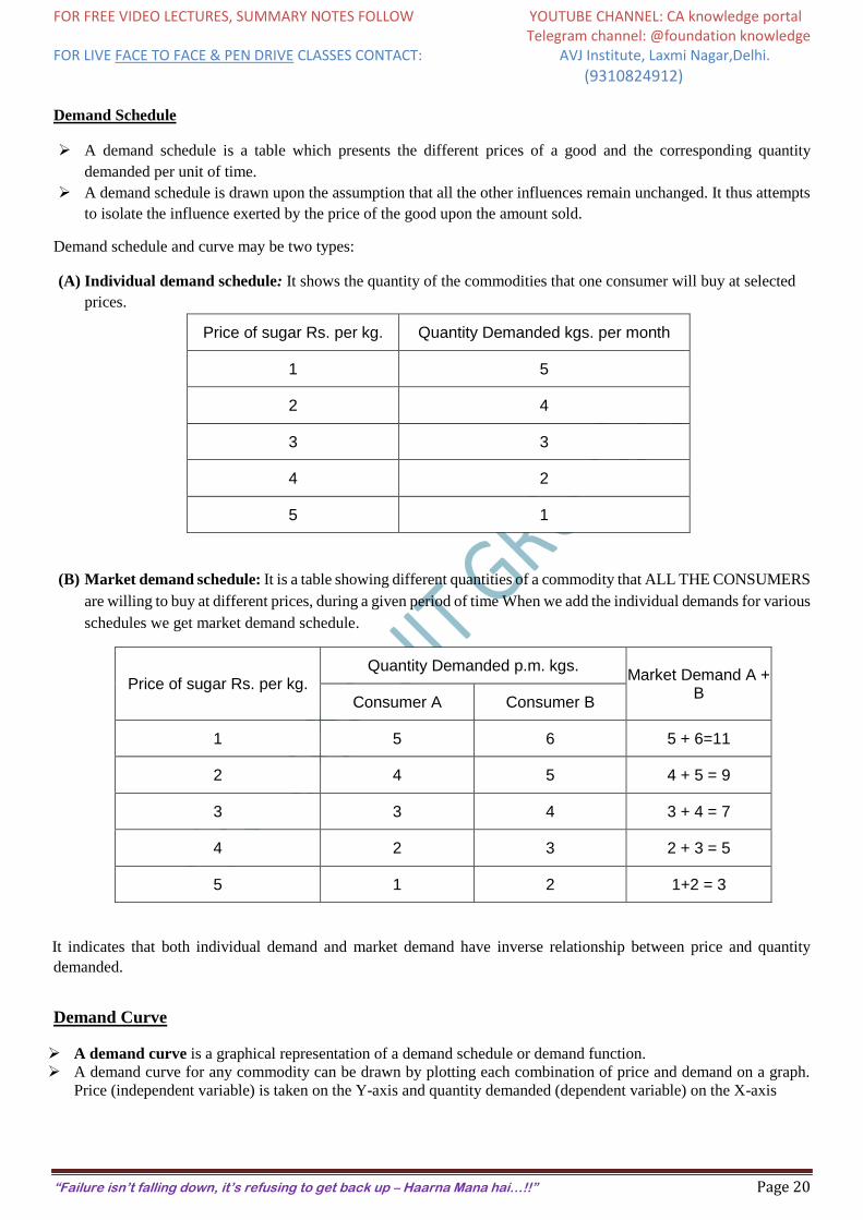
Demand Curve
A demand curve is a graphical representation of a demand schedule or demand function.
A demand curve for any commodity can be drawn by plotting each combination of price and demand on a graph.
Price (independent variable) is taken on the Y-axis and quantity demanded (dependent variable) on the X-axis
FOR FREE VIDEO LECTURES, SUMMARY NOTES FOLLOW YOUTUBE CHANNEL: CA knowledge portal Telegram channel: @foundation knowledge FOR LIVE FACE TO FACE & PEN DRIVE CLASSES CONTACT: AVJ Institute, Laxmi Nagar,Delhi.
(9310824912)
“Failure isn’t falling down, it’s refusing to get back up – Haarna Mana hai…!!” Page 21
Remember:- Market Demand Curve is flatter than individual Demand Curve
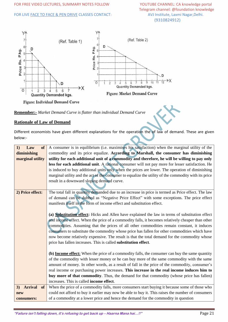
Rationale of Law of Demand
Different economists have given different explanations for the operation the of law of demand. These are given
below:-
1) Law of
diminishing
marginal utility
A consumer is in equilibrium (i.e. maximises his satisfaction) when the marginal utility of the
commodity and its price equalize. According to Marshall, the consumer has diminishing
utility for each additional unit of a commodity and therefore, he will be willing to pay only
less for each additional unit. A rational consumer will not pay more for lesser satisfaction. He
is induced to buy additional units only when the prices are lower. The operation of diminishing
marginal utility and the act of the consumer to equalize the utility of the commodity with its price
result in a downward sloping demand curve.
2) Price effect: The total fall in quantity demanded due to an increase in price is termed as Price effect. The law
of demand can be dubbed as “Negative Price Effect” with some exceptions. The price effect
manifests itself in the form of income effect and substitution effect.
(a) Substitution effect: Hicks and Allen have explained the law in terms of substitution effect
and income effect. When the price of a commodity falls, it becomes relatively cheaper than other
commodities. Assuming that the prices of all other commodities remain constant, it induces
consumers to substitute the commodity whose price has fallen for other commodities which have
now become relatively expensive. The result is that the total demand for the commodity whose
price has fallen increases. This is called substitution effect.
(b) Income effect: When the price of a commodity falls, the consumer can buy the same quantity
of the commodity with lesser money or he can buy more of the same commodity with the same
amount of money. In other words, as a result of fall in the price of the commodity, consumer’s
real income or purchasing power increases. This increase in the real income induces him to
buy more of that commodity. Thus, the demand for that commodity (whose price has fallen)
increases. This is called income effect.
3) Arrival of
new
consumers:
When the price of a commodity falls, more consumers start buying it because some of those who
could not afford to buy it earlier may now be able to buy it. This raises the number of consumers
of a commodity at a lower price and hence the demand for the commodity in question
FOR FREE VIDEO LECTURES, SUMMARY NOTES FOLLOW YOUTUBE CHANNEL: CA knowledge portal Telegram channel: @foundation knowledge FOR LIVE FACE TO FACE & PEN DRIVE CLASSES CONTACT: AVJ Institute, Laxmi Nagar,Delhi.
(9310824912)
“Failure isn’t falling down, it’s refusing to get back up – Haarna Mana hai…!!” Page 22
(4) Different
uses
Certain commodities have multiple uses. If their prices fall, they will be used for varied purposes
and therefore their demand for such commodities will increase. When the price of such
commodities are high (or rises) they will be put to limited uses only. Thus, different uses of a
commodity make the demand curve slope downwards reacting to changes in price. For example
Olive oil can be used for cooking as well as for cosmetic purposes. So if the price of olive oil rises
we can limit our usage and thus the demand will fall
Exceptions to the Law of Demand
The law of demand is valid in most cases; however there are certain cases where this law does not hold good. The
following are the important exceptions to the law of demand.
Conspicuous
goods:
Articles of prestige value or snob appeal or articles of conspicuous consumption are demanded only
by the rich people and these articles become more attractive if their prices go up. Such articles will
not conform to the usual law of demand. This was found out by Veblen in his doctrine of
“Conspicuous Consumption” and hence this effect is called Veblen effect or prestige goods effect.
Veblen effect takes place as some consumers measure the utility of a commodity by its price i.e., if
the commodity is expensive they think that it has got more utility. As such, they buy less of this
commodity at low price and more of it at high price. Diamonds are often given as an example of this
case. Higher the price of diamonds, higher is the prestige value attached to them and hence higher is
the demand for them
Giffen
Goods
Sir Robert Giffen, a Scottish economist and statistician, was surprised to find out that as the price of
bread increased, the British workers purchased more bread and not less of it. This was something
against the law of demand. Why did this happen? The reason given for this is that when the price of
bread went up, it caused such a large decline in the purchasing power of the poor people that they
were forced to cut down the consumption of meat and other more expensive foods. Since bread, even
when its price was higher than before, was still the cheapest food article, people consumed more of
it and not less when its price went up.
Such goods which exhibit direct price-demand relationship are called ‘Giffen goods’. Generally those
goods which are inferior, with no close substitutes easily available and which occupy a substantial
place in consumer’s budget are called ‘Giffen goods’. All Giffen goods are inferior goods; but all
inferior goods are not Giffen goods. Inferior goods ought to have a close substitute. Moreover, the
concept of inferior goods is related to the income of the consumer i.e. the quantity demanded of an
inferior good falls as income rises, price remaining constant as against the concept of giffen goods
which is related to the price of the product itself. Examples of Giffen goods are coarse grains like
bajra, low quality rice and wheat etc.
Conspicuous
necessities:
The demand for certain goods is affected by the demonstration effect of the consumption pattern of
a social group to which an individual belongs. These goods, due to their constant usage, become
necessities of life. For example, in spite of the fact that the prices of television sets, refrigerators,
coolers, cooking gas etc. have been continuously rising, their demand does not show any tendency
to fall.
Future
expectations
about prices:
It has been observed that when the prices are rising, households expecting that the prices in the future
will be still higher, tend to buy larger quantities of such commodities. For example, when there is
wide-spread drought, people expect that prices of food grains would rise in future. They demand
greater quantities of food grains as their price rise. However, it is to be noted that here it is not the
law of demand which is invalidated but there is a change in one of the factors which was held constant
while deriving the law of demand, namely change in the price expectations of the people
FOR FREE VIDEO LECTURES, SUMMARY NOTES FOLLOW YOUTUBE CHANNEL: CA knowledge portal Telegram channel: @foundation knowledge FOR LIVE FACE TO FACE & PEN DRIVE CLASSES CONTACT: AVJ Institute, Laxmi Nagar,Delhi.
(9310824912)
“Failure isn’t falling down, it’s refusing to get back up – Haarna Mana hai…!!” Page 23
Irrational
behaviour of
Consumers
The law has been derived assuming consumers to be rational and knowledgeable about market-
conditions. However, at times, consumers tend to be irrational and make impulsive purchases without
any rational calculations about the price and usefulness of the product and in such contexts the law
of demand fails.
Demand for
necessaries:
The law of demand does not apply much in the case of necessaries of life. Irrespective of price
changes, people have to consume the minimum quantities of necessary commodities. Similarly, in
practice, a household may demand larger quantity of a commodity even at a higher price because it
may be ignorant of the ruling price of the commodity. Under such circumstances, the law will not
remain valid. For example Food, power, water, gas
Speculative
goods:
In the speculative market, particularly in the market for stocks and shares, more will be demanded
when the prices are rising and less will be demanded when prices decline.
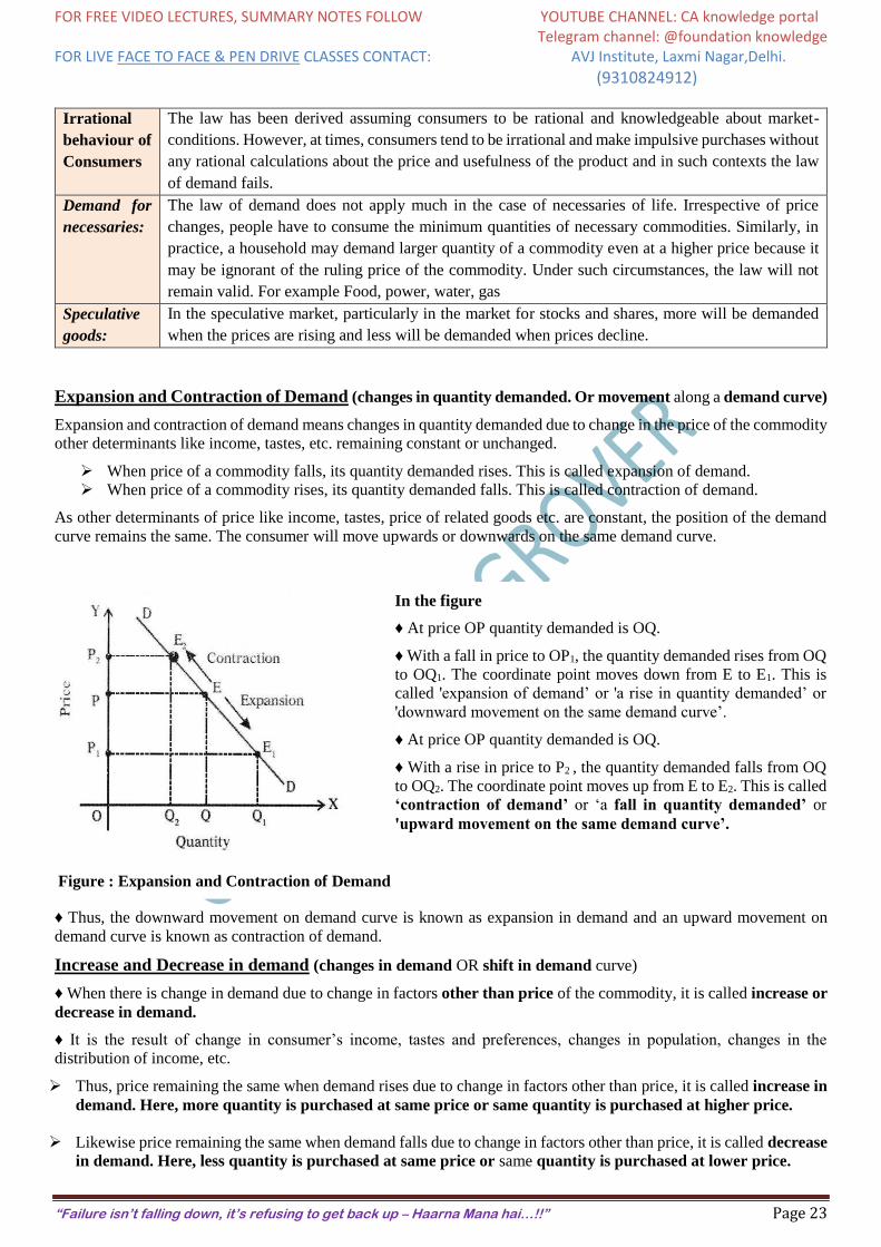
Expansion and Contraction of Demand (changes in quantity demanded. Or movement along a demand curve)
Expansion and contraction of demand means changes in quantity demanded due to change in the price of the commodity
other determinants like income, tastes, etc. remaining constant or unchanged.
When price of a commodity falls, its quantity demanded rises. This is called expansion of demand.
When price of a commodity rises, its quantity demanded falls. This is called contraction of demand.
As other determinants of price like income, tastes, price of related goods etc. are constant, the position of the demand
curve remains the same. The consumer will move upwards or downwards on the same demand curve.
In the figure
♦ At price OP quantity demanded is OQ.
♦ With a fall in price to OP1, the quantity demanded rises from OQ
to OQ1. The coordinate point moves down from E to E1. This is
called 'expansion of demand’ or 'a rise in quantity demanded’ or
'downward movement on the same demand curve’.
♦ At price OP quantity demanded is OQ.
♦ With a rise in price to P2 , the quantity demanded falls from OQ
to OQ2. The coordinate point moves up from E to E2. This is called
‘contraction of demand’ or ‘a fall in quantity demanded’ or
'upward movement on the same demand curve’.
Figure : Expansion and Contraction of Demand
♦ Thus, the downward movement on demand curve is known as expansion in demand and an upward movement on
demand curve is known as contraction of demand.
Increase and Decrease in demand (changes in demand OR shift in demand curve)
♦ When there is change in demand due to change in factors other than price of the commodity, it is called increase or
decrease in demand.
♦ It is the result of change in consumer’s income, tastes and preferences, changes in population, changes in the
distribution of income, etc.
Thus, price remaining the same when demand rises due to change in factors other than price, it is called increase in
demand. Here, more quantity is purchased at same price or same quantity is purchased at higher price.
Likewise price remaining the same when demand falls due to change in factors other than price, it is called decrease
in demand. Here, less quantity is purchased at same price or same quantity is purchased at lower price.
FOR FREE VIDEO LECTURES, SUMMARY NOTES FOLLOW YOUTUBE CHANNEL: CA knowledge portal Telegram channel: @foundation knowledge FOR LIVE FACE TO FACE & PEN DRIVE CLASSES CONTACT: AVJ Institute, Laxmi Nagar,Delhi.
(9310824912)
“Failure isn’t falling down, it’s refusing to get back up – Haarna Mana hai…!!” Page 24
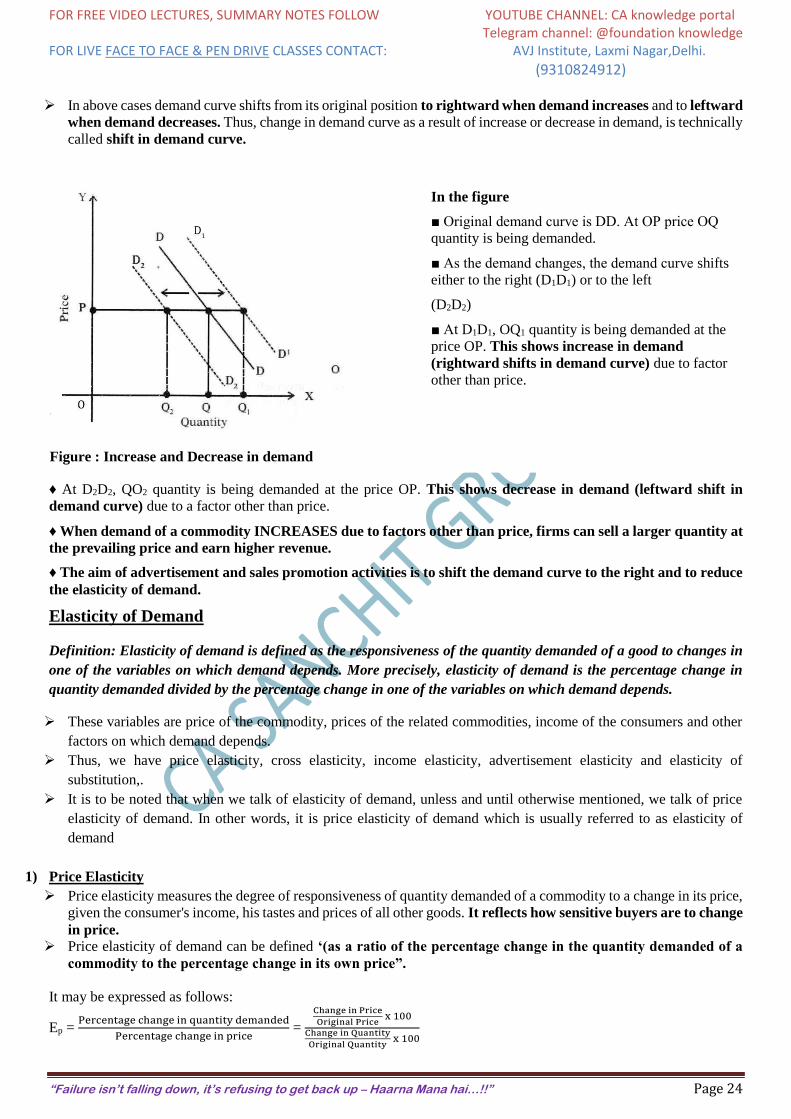
In above cases demand curve shifts from its original position to rightward when demand increases and to leftward
when demand decreases. Thus, change in demand curve as a result of increase or decrease in demand, is technically
called shift in demand curve.
In the figure
■ Original demand curve is DD. At OP price OQ
quantity is being demanded.
■ As the demand changes, the demand curve shifts
either to the right (D1D1) or to the left
(D2D2)
■ At D1D1, OQ1 quantity is being demanded at the
price OP. This shows increase in demand
(rightward shifts in demand curve) due to factor
other than price.
Figure : Increase and Decrease in demand
♦ At D2D2, QO2 quantity is being demanded at the price OP. This shows decrease in demand (leftward shift in
demand curve) due to a factor other than price.
♦ When demand of a commodity INCREASES due to factors other than price, firms can sell a larger quantity at
the prevailing price and earn higher revenue.
♦ The aim of advertisement and sales promotion activities is to shift the demand curve to the right and to reduce
the elasticity of demand.
Elasticity of Demand
Definition: Elasticity of demand is defined as the responsiveness of the quantity demanded of a good to changes in
one of the variables on which demand depends. More precisely, elasticity of demand is the percentage change in
quantity demanded divided by the percentage change in one of the variables on which demand depends.
These variables are price of the commodity, prices of the related commodities, income of the consumers and other
factors on which demand depends.
Thus, we have price elasticity, cross elasticity, income elasticity, advertisement elasticity and elasticity of
substitution,.
It is to be noted that when we talk of elasticity of demand, unless and until otherwise mentioned, we talk of price
elasticity of demand. In other words, it is price elasticity of demand which is usually referred to as elasticity of
demand
1) Price Elasticity
Price elasticity measures the degree of responsiveness of quantity demanded of a commodity to a change in its price,
given the consumer's income, his tastes and prices of all other goods. It reflects how sensitive buyers are to change
in price. Price elasticity of demand can be defined ‘(as a ratio of the percentage change in the quantity demanded of a
commodity to the percentage change in its own price”.
It may be expressed as follows:
Ep = Percentage change in quantity demanded
Percentage change in price =
Change in Price
Original Price x 100
Change in Quantity
Original Quantity x 100
FOR FREE VIDEO LECTURES, SUMMARY NOTES FOLLOW YOUTUBE CHANNEL: CA knowledge portal Telegram channel: @foundation knowledge FOR LIVE FACE TO FACE & PEN DRIVE CLASSES CONTACT: AVJ Institute, Laxmi Nagar,Delhi.
(9310824912)
“Failure isn’t falling down, it’s refusing to get back up – Haarna Mana hai…!!” Page 25
Change in Quantity demanded
Quantity demanded ÷
Change in Price
Price
= Ep = ∆q
q ÷
∆p
P
Rearranging the above expression we get:
EP = ∆q
q ×
P
∆p =
∆q
∆p ×
P
q
Where—
q = Original quantity demanded
p = Original price
Δ = indicates change
Ep = price elasticity
Remember:- Since price and quantity demanded are inversely related, the value of price elasticity coefficient will
always be negative. But for the value of elasticity coefficients we ignore the negative sign and consider the numerical
value only.
Illustrations
Illustration 1:- The price of a commodity decreases from Rs. 6 to Rs. 4 and quantity demanded of the good increases
from 10 units to 15 units. Find the coefficient of price elasticity.
Solution: Price elasticity = (-) Δ q / Δ p × p/q = 5/2 × 6/10 = (-) 1.5
Illustration 2:- A 5% fall in the price of a good leads to a 15% rise in its demand. Determine the elasticity and
comment on its value.
Solution :- Price elasticity = Percentage change in quantity demanded Percentage change in price = 15% / 5% = 3
Comment: The good in question has elastic demand.
Illustration 3:- The price of a good decreases from Rs. 100 to Rs. 60 per unit. If the price elasticity of demand for it
is 1.5 and the original quantity demanded is 30 units, calculate the new quantity demanded.
Solution:- Ep = _q/_p * p/q , Here Δ q 40 100 30 x = 1.5 1.5 x 1200 100 = = 18 Δ q
Therefore new quantity demanded = 30+18 = 48 units.
The degrees (types) of price elasticity of demand.
Price elasticity measures the degree of responsiveness of quantity demanded of a commodity to a change in its price.
Depending upon the degree of responsiveness of the quantity demanded to the price changes, we can have the following
kinds of price elasticity of demand.
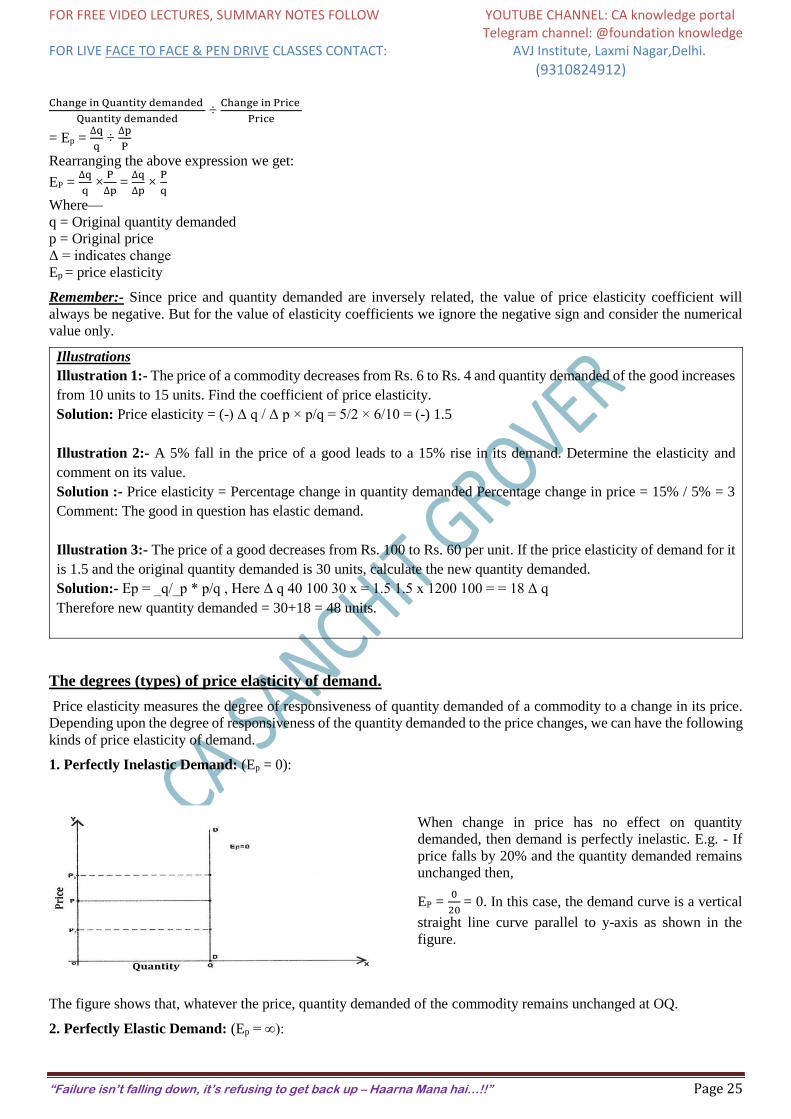
1. Perfectly Inelastic Demand: (Ep = 0):
When change in price has no effect on quantity
demanded, then demand is perfectly inelastic. E.g. - If
price falls by 20% and the quantity demanded remains
unchanged then,
EP = 0
20 = 0. In this case, the demand curve is a vertical
straight line curve parallel to y-axis as shown in the
figure.
The figure shows that, whatever the price, quantity demanded of the commodity remains unchanged at OQ.
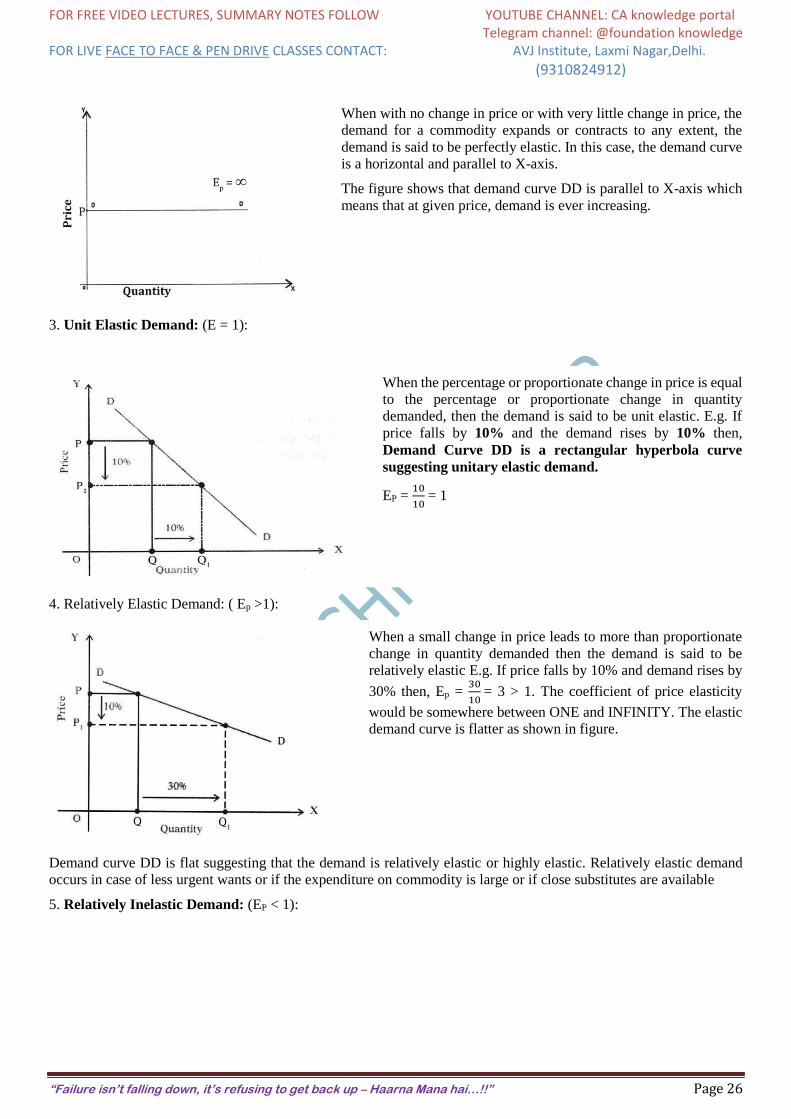
2. Perfectly Elastic Demand: (Ep = ∞):
FOR FREE VIDEO LECTURES, SUMMARY NOTES FOLLOW YOUTUBE CHANNEL: CA knowledge portal Telegram channel: @foundation knowledge FOR LIVE FACE TO FACE & PEN DRIVE CLASSES CONTACT: AVJ Institute, Laxmi Nagar,Delhi.
(9310824912)
“Failure isn’t falling down, it’s refusing to get back up – Haarna Mana hai…!!” Page 26
When with no change in price or with very little change in price, the
demand for a commodity expands or contracts to any extent, the
demand is said to be perfectly elastic. In this case, the demand curve
is a horizontal and parallel to X-axis.
The figure shows that demand curve DD is parallel to X-axis which
means that at given price, demand is ever increasing.
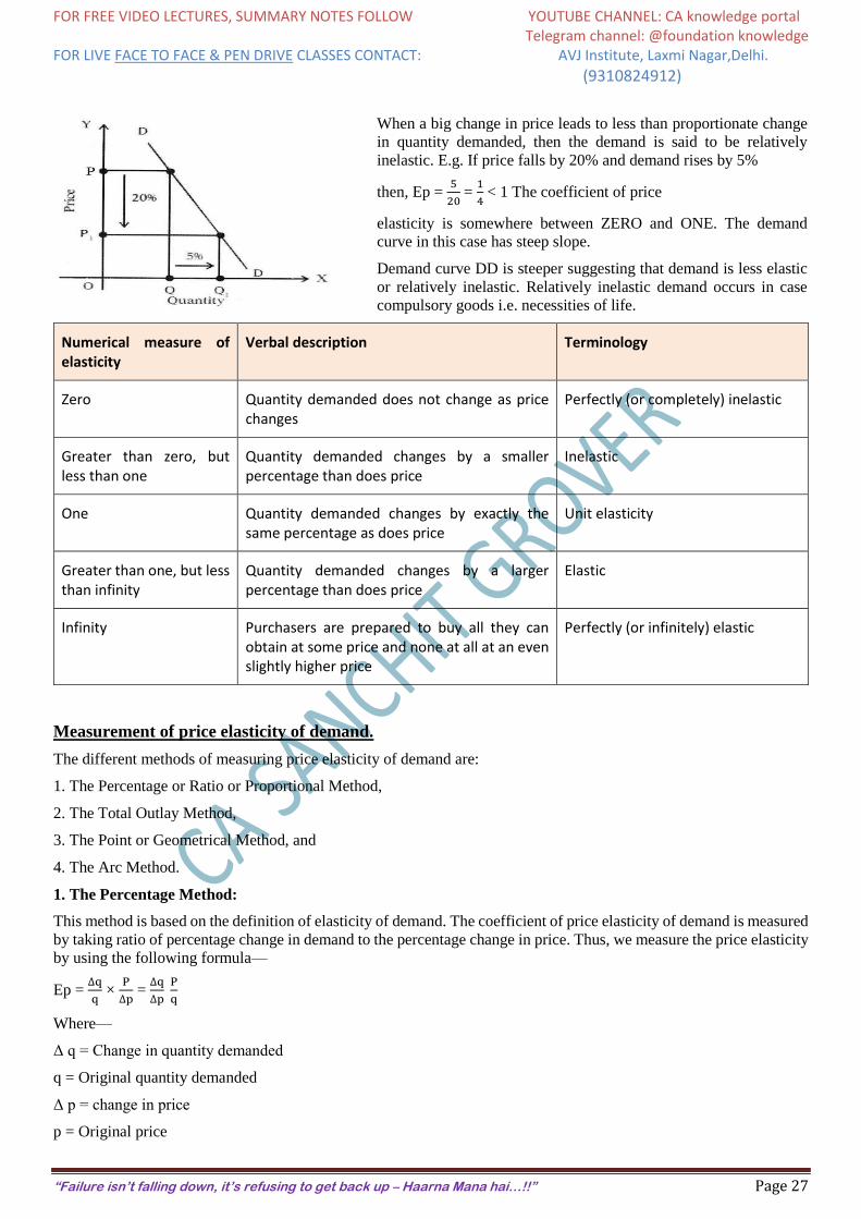
3. Unit Elastic Demand: (E = 1):
When the percentage or proportionate change in price is equal
to the percentage or proportionate change in quantity
demanded, then the demand is said to be unit elastic. E.g. If
price falls by 10% and the demand rises by 10% then,
Demand Curve DD is a rectangular hyperbola curve
suggesting unitary elastic demand.
EP = 10
10 = 1
4. Relatively Elastic Demand: ( Ep >1):
When a small change in price leads to more than proportionate
change in quantity demanded then the demand is said to be
relatively elastic E.g. If price falls by 10% and demand rises by
30% then, Ep = 30
10 = 3 > 1. The coefficient of price elasticity
would be somewhere between ONE and INFINITY. The elastic
demand curve is flatter as shown in figure.
Demand curve DD is flat suggesting that the demand is relatively elastic or highly elastic. Relatively elastic demand
occurs in case of less urgent wants or if the expenditure on commodity is large or if close substitutes are available
5. Relatively Inelastic Demand: (EP < 1):
FOR FREE VIDEO LECTURES, SUMMARY NOTES FOLLOW YOUTUBE CHANNEL: CA knowledge portal Telegram channel: @foundation knowledge FOR LIVE FACE TO FACE & PEN DRIVE CLASSES CONTACT: AVJ Institute, Laxmi Nagar,Delhi.
(9310824912)
“Failure isn’t falling down, it’s refusing to get back up – Haarna Mana hai…!!” Page 27
When a big change in price leads to less than proportionate change
in quantity demanded, then the demand is said to be relatively
inelastic. E.g. If price falls by 20% and demand rises by 5%
then, Ep = 5
20 =
1
4 < 1 The coefficient of price
elasticity is somewhere between ZERO and ONE. The demand
curve in this case has steep slope.
Demand curve DD is steeper suggesting that demand is less elastic
or relatively inelastic. Relatively inelastic demand occurs in case
compulsory goods i.e. necessities of life.
Numerical measure of elasticity
Verbal description Terminology
Zero Quantity demanded does not change as price changes
Perfectly (or completely) inelastic
Greater than zero, but less than one
Quantity demanded changes by a smaller percentage than does price
Inelastic
One Quantity demanded changes by exactly the same percentage as does price
Unit elasticity
Greater than one, but less than infinity
Quantity demanded changes by a larger percentage than does price
Elastic
Infinity Purchasers are prepared to buy all they can obtain at some price and none at all at an even slightly higher price
Perfectly (or infinitely) elastic
Measurement of price elasticity of demand.
The different methods of measuring price elasticity of demand are:
1. The Percentage or Ratio or Proportional Method,
2. The Total Outlay Method,
3. The Point or Geometrical Method, and
4. The Arc Method.
1. The Percentage Method:
This method is based on the definition of elasticity of demand. The coefficient of price elasticity of demand is measured
by taking ratio of percentage change in demand to the percentage change in price. Thus, we measure the price elasticity
by using the following formula—
Ep = ∆q
q ×
P
∆p =
∆q
∆p P
q
Where—
Δ q = Change in quantity demanded
q = Original quantity demanded
Δ p = change in price
p = Original price
FOR FREE VIDEO LECTURES, SUMMARY NOTES FOLLOW YOUTUBE CHANNEL: CA knowledge portal Telegram channel: @foundation knowledge FOR LIVE FACE TO FACE & PEN DRIVE CLASSES CONTACT: AVJ Institute, Laxmi Nagar,Delhi.
(9310824912)
“Failure isn’t falling down, it’s refusing to get back up – Haarna Mana hai…!!” Page 28
If the coefficient of above ratio is equal to ONE or UNITY, the demand will be unitary.
If the coefficient of above ratio is MORE THAN ONE, the demand is relatively elastic.
If the coefficient of above ratio is LESS THAN ONE, the demand is relatively inelastic.
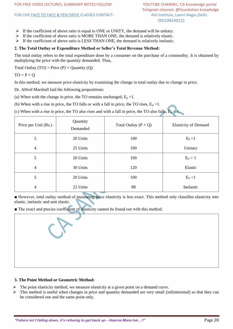
2. The Total Outlay or Expenditure Method or Seller’s Total Revenue Method:
The total outlay refers to the total expenditure done by a consumer on the purchase of a commodity. It is obtained by
multiplying the price with the quantity demanded. Thus,
Total Outlay (TO) = Price (P) × Quantity (Q)
TO = P × Q
In this method, we measure price elasticity by examining the change in total outlay due to change in price.
Dr. Alfred Marshall laid the following propositions:
(a) When with the change in price, the TO remains unchanged, Ep =1.
(b) When with a rise in price, the TO falls or with a fall in price, the TO rises, Ep >1.
(c) When with a rise in price, the TO also rises and with a fall in price, the TO also falls, Ep < 1.
Price per Unit (Rs.) Quantity
Demanded Total Outlay (P × Q) Elasticity of Demand
5 20 Units 100 EP =1
4 25 Units 100 Unitary
5 20 Units 100 EP > 1
4 30 Units 120 Elastic
5 20 Units 100 EP <1
4 22 Units 88 Inelastic
■ However, total outlay method of measuring price elasticity is less exact. This method only classifies elasticity into
elastic, inelastic and unit elastic.
■ The exact and precise coefficient of elasticity cannot be found out with this method.
3. The Point Method or Geometric Method:
The point elasticity method, we measure elasticity at a given point on a demand curve.
This method is useful when changes in price and quantity demanded are very small (infinitesimal) so that they can
be considered one and the same point only.
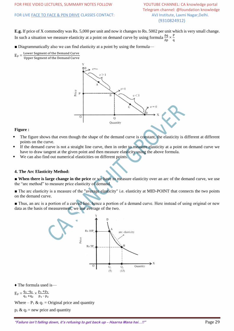
FOR FREE VIDEO LECTURES, SUMMARY NOTES FOLLOW YOUTUBE CHANNEL: CA knowledge portal Telegram channel: @foundation knowledge FOR LIVE FACE TO FACE & PEN DRIVE CLASSES CONTACT: AVJ Institute, Laxmi Nagar,Delhi.
(9310824912)
“Failure isn’t falling down, it’s refusing to get back up – Haarna Mana hai…!!” Page 29
E.g. If price of X commodity was Rs. 5,000 per unit and now it changes to Rs. 5002 per unit which is very small change.
In such a situation we measure elasticity at a point on demand curve by using formula ∆q
∆p ×
P
q
■ Diagrammatically also we can find elasticity at a point by using the formula—
EP = Lower Segment of the Demand Curve
Upper Segment of the Demand Curve
Figure :
The figure shows that even though the shape of the demand curve is constant, the elasticity is different at different
points on the curve.
If the demand curve is not a straight line curve, then in order to measure elasticity at a point on demand curve we
have to draw tangent at the given point and then measure elasticity using the above formula.
We can also find out numerical elasticities on different points.
4. The Arc Elasticity Method:
■ When there is large change in the price or we have to measure elasticity over an arc of the demand curve, we use
the “arc method” to measure price elasticity of demand.
■ The arc elasticity is a measure of the "average elasticity" i.e. elasticity at MID-POINT that connects the two points
on the demand curve.
■ Thus, an arc is a portion of a curved line, hence a portion of a demand curve. Here instead of using original or new
data as the basis of measurement, we use average of the two.
♦ The formula used is—
EP = q1 –q2
q1 +q2 ×
p1 +p2
p1 – p2
Where – P1 & q1 = Original price and quantity
p2 & q2 = new price and quantity
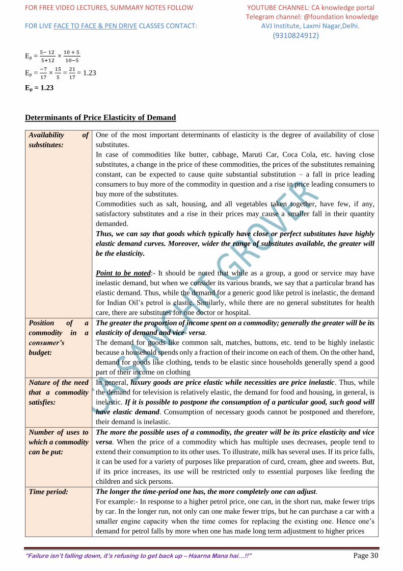
FOR FREE VIDEO LECTURES, SUMMARY NOTES FOLLOW YOUTUBE CHANNEL: CA knowledge portal Telegram channel: @foundation knowledge FOR LIVE FACE TO FACE & PEN DRIVE CLASSES CONTACT: AVJ Institute, Laxmi Nagar,Delhi.
(9310824912)
“Failure isn’t falling down, it’s refusing to get back up – Haarna Mana hai…!!” Page 30
Ep = 5− 12
5+12 ×
10 + 5
10−5
Ep = −7
17 ×
15
5 =
21
17 = 1.23
Ep = 1.23
Determinants of Price Elasticity of Demand
Availability of
substitutes:
One of the most important determinants of elasticity is the degree of availability of close
substitutes.
In case of commodities like butter, cabbage, Maruti Car, Coca Cola, etc. having close
substitutes, a change in the price of these commodities, the prices of the substitutes remaining
constant, can be expected to cause quite substantial substitution – a fall in price leading
consumers to buy more of the commodity in question and a rise in price leading consumers to
buy more of the substitutes.
Commodities such as salt, housing, and all vegetables taken together, have few, if any,
satisfactory substitutes and a rise in their prices may cause a smaller fall in their quantity
demanded.
Thus, we can say that goods which typically have close or perfect substitutes have highly
elastic demand curves. Moreover, wider the range of substitutes available, the greater will
be the elasticity.
Point to be noted:- It should be noted that while as a group, a good or service may have
inelastic demand, but when we consider its various brands, we say that a particular brand has
elastic demand. Thus, while the demand for a generic good like petrol is inelastic, the demand
for Indian Oil’s petrol is elastic. Similarly, while there are no general substitutes for health
care, there are substitutes for one doctor or hospital.
Position of a
commodity in a
consumer’s
budget:
The greater the proportion of income spent on a commodity; generally the greater will be its
elasticity of demand and vice- versa.
The demand for goods like common salt, matches, buttons, etc. tend to be highly inelastic
because a household spends only a fraction of their income on each of them. On the other hand,
demand for goods like clothing, tends to be elastic since households generally spend a good
part of their income on clothing
Nature of the need
that a commodity
satisfies:
In general, luxury goods are price elastic while necessities are price inelastic. Thus, while
the demand for television is relatively elastic, the demand for food and housing, in general, is
inelastic. If it is possible to postpone the consumption of a particular good, such good will
have elastic demand. Consumption of necessary goods cannot be postponed and therefore,
their demand is inelastic.
Number of uses to
which a commodity
can be put:
The more the possible uses of a commodity, the greater will be its price elasticity and vice
versa. When the price of a commodity which has multiple uses decreases, people tend to
extend their consumption to its other uses. To illustrate, milk has several uses. If its price falls,
it can be used for a variety of purposes like preparation of curd, cream, ghee and sweets. But,
if its price increases, its use will be restricted only to essential purposes like feeding the
children and sick persons.
Time period: The longer the time-period one has, the more completely one can adjust.
For example:- In response to a higher petrol price, one can, in the short run, make fewer trips
by car. In the longer run, not only can one make fewer trips, but he can purchase a car with a
smaller engine capacity when the time comes for replacing the existing one. Hence one’s
demand for petrol falls by more when one has made long term adjustment to higher prices
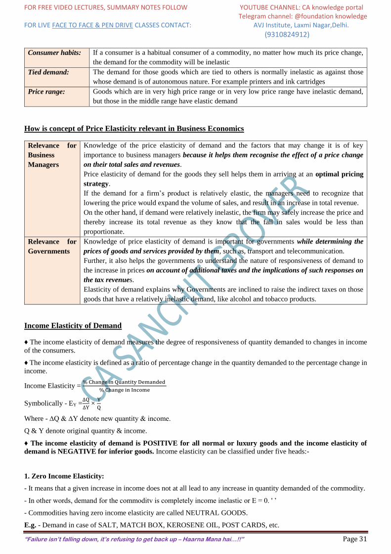
FOR FREE VIDEO LECTURES, SUMMARY NOTES FOLLOW YOUTUBE CHANNEL: CA knowledge portal Telegram channel: @foundation knowledge FOR LIVE FACE TO FACE & PEN DRIVE CLASSES CONTACT: AVJ Institute, Laxmi Nagar,Delhi.
(9310824912)
“Failure isn’t falling down, it’s refusing to get back up – Haarna Mana hai…!!” Page 31
Consumer habits: If a consumer is a habitual consumer of a commodity, no matter how much its price change,
the demand for the commodity will be inelastic
Tied demand: The demand for those goods which are tied to others is normally inelastic as against those
whose demand is of autonomous nature. For example printers and ink cartridges
Price range: Goods which are in very high price range or in very low price range have inelastic demand,
but those in the middle range have elastic demand
How is concept of Price Elasticity relevant in Business Economics
Relevance for
Business
Managers
Knowledge of the price elasticity of demand and the factors that may change it is of key
importance to business managers because it helps them recognise the effect of a price change
on their total sales and revenues.
Price elasticity of demand for the goods they sell helps them in arriving at an optimal pricing
strategy.
If the demand for a firm’s product is relatively elastic, the managers need to recognize that
lowering the price would expand the volume of sales, and result in an increase in total revenue.
On the other hand, if demand were relatively inelastic, the firm may safely increase the price and
thereby increase its total revenue as they know that the fall in sales would be less than
proportionate.
Relevance for
Governments
Knowledge of price elasticity of demand is important for governments while determining the
prices of goods and services provided by them, such as, transport and telecommunication.
Further, it also helps the governments to understand the nature of responsiveness of demand to
the increase in prices on account of additional taxes and the implications of such responses on
the tax revenues.
Elasticity of demand explains why Governments are inclined to raise the indirect taxes on those
goods that have a relatively inelastic demand, like alcohol and tobacco products.
Income Elasticity of Demand
♦ The income elasticity of demand measures the degree of responsiveness of quantity demanded to changes in income
of the consumers.
♦ The income elasticity is defined as a ratio of percentage change in the quantity demanded to the percentage change in
income.
Income Elasticity = % Change in Quantity Demanded
% Change in Income
Symbolically - EY =∆Q
∆Y ×
Y
Q
Where - ∆Q & ∆Y denote new quantity & income.
Q & Y denote original quantity & income.
♦ The income elasticity of demand is POSITIVE for all normal or luxury goods and the income elasticity of
demand is NEGATIVE for inferior goods. Income elasticity can be classified under five heads:-
1. Zero Income Elasticity:
- It means that a given increase in income does not at all lead to any increase in quantity demanded of the commodity.
- In other words, demand for the commoditv is completely income inelastic or E = 0. ' ’
- Commodities having zero income elasticity are called NEUTRAL GOODS.
E.g. - Demand in case of SALT, MATCH BOX, KEROSENE OIL, POST CARDS, etc.
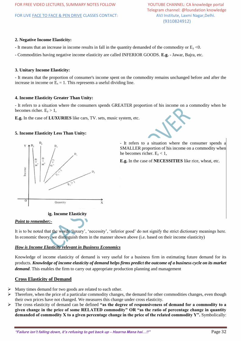
FOR FREE VIDEO LECTURES, SUMMARY NOTES FOLLOW YOUTUBE CHANNEL: CA knowledge portal Telegram channel: @foundation knowledge FOR LIVE FACE TO FACE & PEN DRIVE CLASSES CONTACT: AVJ Institute, Laxmi Nagar,Delhi.
(9310824912)
“Failure isn’t falling down, it’s refusing to get back up – Haarna Mana hai…!!” Page 32
2. Negative Income Elasticity:
- It means that an increase in income results in fall in the quantity demanded of the commodity or Ey <0.
- Commodities having negative income elasticity are called INFERIOR GOODS. E.g. - Jawar, Bajra, etc.
3. Unitary Income Elasticity:
- It means that the proportion of consumer's income spent on the commodity remains unchanged before and after the
increase in income or Es = 1. This represents a useful dividing line.
4. Income Elasticity Greater Than Unity:
- It refers to a situation where the consumers spends GREATER proportion of his income on a commodity when he
becomes richer. Ey > 1,
E.g. In the case of LUXURIES like cars, TV. sets, music system, etc.
5. Income Elasticity Less Than Unity:
- It refers to a situation where the consumer spends a
SMALLER proportion of his income on a commodity when
he becomes richer. Ey < 1,
E.g. In the case of NECESSITIES like rice, wheat, etc.
ig. Income Elasticity
Point to remember:-
It is to be noted that the words ‘luxury’, ‘necessity’, ‘inferior good’ do not signify the strict dictionary meanings here.
In economic theory, we distinguish them in the manner shown above (i.e. based on their income elasticity)
How is Income Elasticity relevant in Business Economics
Knowledge of income elasticity of demand is very useful for a business firm in estimating future demand for its
products. Knowledge of income elasticity of demand helps firms predict the outcome of a business cycle on its market
demand. This enables the firm to carry out appropriate production planning and management
Cross Elasticity of Demand
Many times demand for two goods are related to each other.
Therefore, when the price of a particular commodity changes, the demand for other commodities changes, even though
their own prices have not changed. We measures this change under cross elasticity.
The cross elasticity of demand can be defined “as the degree of responsiveness of demand for a commodity to a
given change in the price of some RELATED commodity" OR “as the ratio of percentage change in quantity
demanded of commodity X to a given percentage change in the price of the related commodity Y”. Symbolically:
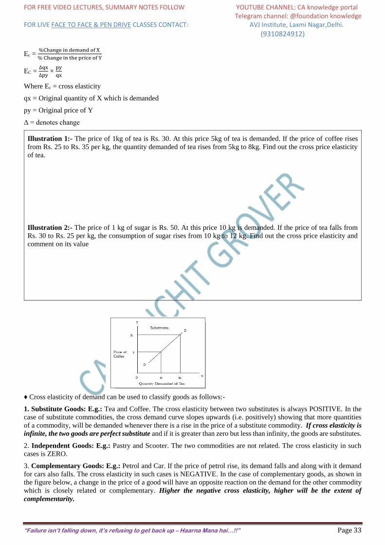
FOR FREE VIDEO LECTURES, SUMMARY NOTES FOLLOW YOUTUBE CHANNEL: CA knowledge portal Telegram channel: @foundation knowledge FOR LIVE FACE TO FACE & PEN DRIVE CLASSES CONTACT: AVJ Institute, Laxmi Nagar,Delhi.
(9310824912)
“Failure isn’t falling down, it’s refusing to get back up – Haarna Mana hai…!!” Page 33
Ec = %Change in demand of X
% Change in the price of Y
EC = ∆qx
∆py ×
py
qx
Where Ec = cross elasticity
qx = Original quantity of X which is demanded
py = Original price of Y
Δ = denotes change
Illustration 1:- The price of 1kg of tea is Rs. 30. At this price 5kg of tea is demanded. If the price of coffee rises
from Rs. 25 to Rs. 35 per kg, the quantity demanded of tea rises from 5kg to 8kg. Find out the cross price elasticity
of tea.
Illustration 2:- The price of 1 kg of sugar is Rs. 50. At this price 10 kg is demanded. If the price of tea falls from
Rs. 30 to Rs. 25 per kg, the consumption of sugar rises from 10 kg to 12 kg. Find out the cross price elasticity and
comment on its value
♦ Cross elasticity of demand can be used to classify goods as follows:-
1. Substitute Goods: E.g.: Tea and Coffee. The cross elasticity between two substitutes is always POSITIVE. In the
case of substitute commodities, the cross demand curve slopes upwards (i.e. positively) showing that more quantities
of a commodity, will be demanded whenever there is a rise in the price of a substitute commodity. If cross elasticity is
infinite, the two goods are perfect substitute and if it is greater than zero but less than infinity, the goods are substitutes.
2. Independent Goods: E.g.: Pastry and Scooter. The two commodities are not related. The cross elasticity in such
cases is ZERO.
3. Complementary Goods: E.g.: Petrol and Car. If the price of petrol rise, its demand falls and along with it demand
for cars also falls. The cross elasticity in such cases is NEGATIVE. In the case of complementary goods, as shown in
the figure below, a change in the price of a good will have an opposite reaction on the demand for the other commodity
which is closely related or complementary. Higher the negative cross elasticity, higher will be the extent of
complementarity.
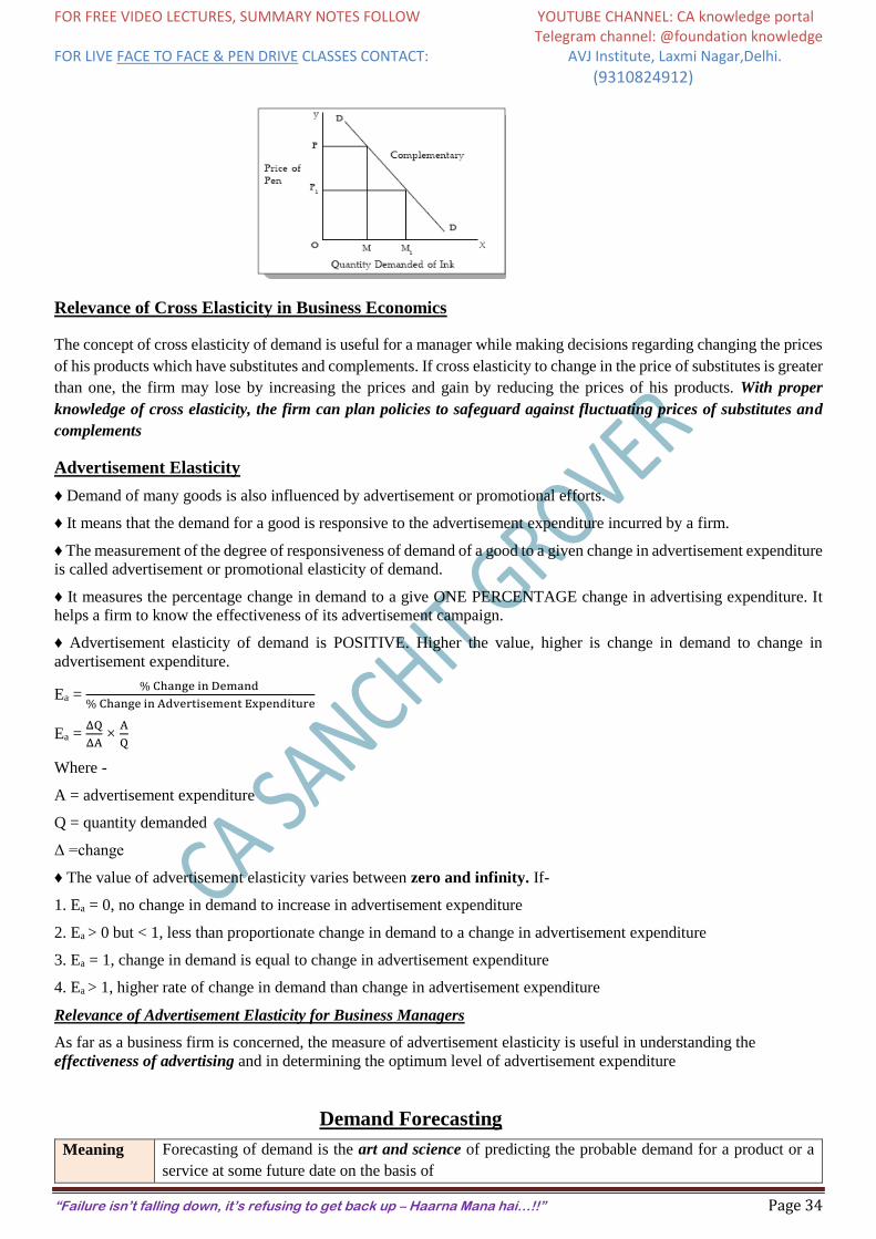
FOR FREE VIDEO LECTURES, SUMMARY NOTES FOLLOW YOUTUBE CHANNEL: CA knowledge portal Telegram channel: @foundation knowledge FOR LIVE FACE TO FACE & PEN DRIVE CLASSES CONTACT: AVJ Institute, Laxmi Nagar,Delhi.
(9310824912)
“Failure isn’t falling down, it’s refusing to get back up – Haarna Mana hai…!!” Page 34
Relevance of Cross Elasticity in Business Economics
The concept of cross elasticity of demand is useful for a manager while making decisions regarding changing the prices
of his products which have substitutes and complements. If cross elasticity to change in the price of substitutes is greater
than one, the firm may lose by increasing the prices and gain by reducing the prices of his products. With proper
knowledge of cross elasticity, the firm can plan policies to safeguard against fluctuating prices of substitutes and
complements
Advertisement Elasticity
♦ Demand of many goods is also influenced by advertisement or promotional efforts.
♦ It means that the demand for a good is responsive to the advertisement expenditure incurred by a firm.
♦ The measurement of the degree of responsiveness of demand of a good to a given change in advertisement expenditure
is called advertisement or promotional elasticity of demand.
♦ It measures the percentage change in demand to a give ONE PERCENTAGE change in advertising expenditure. It
helps a firm to know the effectiveness of its advertisement campaign.
♦ Advertisement elasticity of demand is POSITIVE. Higher the value, higher is change in demand to change in
advertisement expenditure.
Ea = % Change in Demand
% Change in Advertisement Expenditure
Ea = ΔQ
ΔA ×
A
Q
Where -
A = advertisement expenditure
Q = quantity demanded
Δ =change
♦ The value of advertisement elasticity varies between zero and infinity. If-
1. Ea = 0, no change in demand to increase in advertisement expenditure
2. Ea > 0 but < 1, less than proportionate change in demand to a change in advertisement expenditure
3. Ea = 1, change in demand is equal to change in advertisement expenditure
4. Ea > 1, higher rate of change in demand than change in advertisement expenditure
Relevance of Advertisement Elasticity for Business Managers
As far as a business firm is concerned, the measure of advertisement elasticity is useful in understanding the
effectiveness of advertising and in determining the optimum level of advertisement expenditure
Demand Forecasting
Meaning Forecasting of demand is the art and science of predicting the probable demand for a product or a
service at some future date on the basis of
FOR FREE VIDEO LECTURES, SUMMARY NOTES FOLLOW YOUTUBE CHANNEL: CA knowledge portal Telegram channel: @foundation knowledge FOR LIVE FACE TO FACE & PEN DRIVE CLASSES CONTACT: AVJ Institute, Laxmi Nagar,Delhi.
(9310824912)
“Failure isn’t falling down, it’s refusing to get back up – Haarna Mana hai…!!” Page 35
certain past behaviour patterns of some related events and
the prevailing trends in the present.
It should be kept in mind that demand forecasting is no simple guessing, but it refers to estimating
demand scientifically and objectively on the basis of certain facts and events relevant to forecasting.
Why is it useful
Demand forecasting is an important function of managers as it reduces uncertainty of environment in which
DECISIONS are made. Further, it helps in PLANNING for future level of production. Its significance can be stated
as follows:
Production
Planning:
Demand forecasting is a pre-requisite for planning of production in a firm. Expansion of production
capacity depends upon likely demand for its output. Otherwise, there may be overproduction or
underproduction leading to losses
Sales
Forecasting
Sales forecasting depends upon demand forecasting. Promotional efforts of the firm like
advertisements, suitable pricing etc. should be based on demand forecasting
Control of
Business
Demand forecast provide information for budgetary planning and cost control in functional area of
finance and accounting
Inventory
Control
Demand forecasting helps in exercising satisfactory control of business inventories like raw-
materials, intermediate goods, semi-finished goods, spare parts, etc. Estimates of future requirement
of inventories is to be done regularly and it can be known from demand forecasts
Capital
Investments
Capital investments yield returns over many years in future. Decision about investment is to be taken
by comparing rate of return on capital investment and current rate of interest. Demand
forecasting helps in taking investment decisions
Scope of Forecasting
Demand forecasting can be at the international level depending upon the area of operation of the given economic
institution.
It can also be confined to a given product or service supplied by a small firm in a local area.
How to decide the scope
The scope of the forecasting task will depend upon the area of operation of the firm in the present as well as what
is proposed in future.
Much would depend upon the cost and time involved in relation to the benefit of the information acquired through
the study of demand. The necessary trade-off has to be struck between the cost of forecasting and the benefits
flowing from such forecasting.
Types of Forecasts
Based on Scope of Study
Macro-level
forecasting
It deals with the general economic environment prevailing in the economy as measured by the
Index of Industrial Production (IIP), national income and general level of employment etc.
Industry-level
forecasting
It is concerned with the demand for the industry’s products as a whole. For example, demand for
cement in India.
Firm-level
Forecasting
It refers to forecasting the demand for a particular firm’s product, say, the demand for ACC
cement.
Based on time period
Short-term
demand
forecasting
It covers a short span of time, depending of the nature of industry. It is done usually for six months
or less than one year and is generally useful in tactical decisions
FOR FREE VIDEO LECTURES, SUMMARY NOTES FOLLOW YOUTUBE CHANNEL: CA knowledge portal Telegram channel: @foundation knowledge FOR LIVE FACE TO FACE & PEN DRIVE CLASSES CONTACT: AVJ Institute, Laxmi Nagar,Delhi.
(9310824912)
“Failure isn’t falling down, it’s refusing to get back up – Haarna Mana hai…!!” Page 36
Long-term
forecasts
These are for longer periods of time, say two to five years and more. It provides information for
major strategic decisions of the firm such as expansion of plant capacity
Demand Distinction
A) Producer’s goods v/s Consumer’s Goods
Producer’s
Goods
Producer’s goods are those which are used for the production of other goods - either consumer
goods or producer goods themselves. Examples of such goods are machines, plant and equipments
Consumer’s
Goods
Consumer’s goods are those which are used for final consumption. Examples of consumer’s goods
are readymade clothes, prepared food, residential houses, etc.
B) Durable Goods v/s Non-durable goods
Durable
Goods
Durable goods do not quickly wear out, can be consumed more than once and yield utility over a
period of time. Examples of durable consumer goods are: cars, refrigerators and mobile phones.
Building, plant and machinery, office furniture etc are durable producer goods. The demand for
durable goods is likely to be derived demand.
Non-durable
goods
Non-durable goods are those which cannot be consumed more than once. Raw materials, fuel and
power, packing items etc are examples of non-durable producer goods. Beverages, bread, milk etc.
are examples of non-durable consumer goods. These will meet only the current demand.
Semi-durable
goods
Goods like clothes and umbrella are semi-durable in nature since they possess the characteristics
of both types of goods
C) Derived Demand v/s Autonomous Demand
Derived
Demand
The demand for a commodity that arises because of the demand for some other commodity called
‘parent product’, ‘is called derived demand. For example, the demand for cement is derived
demand, being directly related to building activity.
In general, the demand for producer goods or industrial inputs is derived demand. Also the demand
for complementary goods is derived demand
Autonomous
Demand
If the demand for a product is independent of the demand for other goods, then it is called
autonomous demand. It arises on its own out of an innate desire of the consumer to consume or to
possess the commodity
Remember:- This distinction between derived and autonomous demand is purely arbitrary and
it is very difficult to find out which product is entirely independent of other products.
D) Demand for Firm v/s Industry Demand
Industry
Demand
The term industry demand is used to denote the total demand for the products of a particular
industry, e.g. the total demand for steel in the country
Demand for
Firm’s
products
The demand for firm’s product denotes the demand for the products of a particular firm, i.e. the
quantity that a firm can dispose off at a given price over a period of time. E.g. demand for steel
produced by the Tata Iron and Steel Company. The demand for a firm’s product when expressed
as a percentage of industry demand signifies the market share of the firm.
E) Short-run Demand and Long-run Demand
Short run
demand
Short-run demand refers to demand with its immediate reaction to changes in product price and
prices of related commodities, income fluctuations, ability of the consumer to adjust their
consumption pattern, their susceptibility to advertisement of new products etc.
Long-run
demand
Long-run demand refers to demand which exists over a long period. Most generic goods have long-
term demand. Long term demand depends on
long-term income trends,
availability of substitutes,
credit facilities etc.
FOR FREE VIDEO LECTURES, SUMMARY NOTES FOLLOW YOUTUBE CHANNEL: CA knowledge portal Telegram channel: @foundation knowledge FOR LIVE FACE TO FACE & PEN DRIVE CLASSES CONTACT: AVJ Institute, Laxmi Nagar,Delhi.
(9310824912)
“Failure isn’t falling down, it’s refusing to get back up – Haarna Mana hai…!!” Page 37
In short, long-run demand is that which will ultimately exist as a result of changes in pricing,
promotion or product improvement, after enough time is allowed to let the market adjust to the
new situation. For example, if electricity rates are reduced, in the short run, the existing users will
make greater use of electric appliances. In the long-run, more and more people will be induced to
use electric appliances
Analysis of Demand Specific Factors
Factors affecting demand of non-durable consumer goods
Disposable
income:
Other things being equal, the demand for a commodity depends upon the disposable income of the
household. Disposable income is found out by deducting personal taxes from personal income.
Price Other things being equal, the demand for a commodity depends upon its own price and the prices
of related goods (its substitutes and complements). While the demand for a good is inversely related
to its own price and the price of its complements, it is positively related to the price of its substitutes.
Demography This involves the characteristics of the population, human as well as non-human, using the product
concerned. For example, it may pertain to the number and characteristics of children in a study of
demand for toys and characteristics of automobiles in a study of the demand for tyres or petrol
Remember
Non-durables are purchased for current consumption only. From a business firm’s point of view, demand for non-
durable goods gets repeated depending on the nature of the non-durable goods. Usually, non-durable goods come in
wide varieties and there is competition among the sellers to acquire and retain customer loyalty
Factors affecting demand of durable-consumer goods
Postponement
of demand
A consumer can postpone the replacement of durable goods. Whether a consumer will go on using
the good for a long time or will replace it depends upon factors like his social status, prestige, level
of money income, rate of obsolescence etc.
Special
facilities
These goods require special facilities for their use e.g. roads for automobiles, and electricity for
refrigerators and radios. The existence and growth of such factors is an important variable that
determines the demand for durable goods
Impact of
Households
As consumer durables are used by more than one person, the decision to purchase may be in_uenced
by family characteristics like income of the family, size, age distribution and sex composition.
Likely changes in the number of households should be considered while determining the market
size of durable goods.
Replacement
demand
Replacement demand is an important component of the total demand for durables. Greater the
current holdings of durable goods, greater will be the replacement demand. Therefore, all factors
that determine replacement demand should be considered as a determinant of the demand for
durable goods
Prices and
Credit
availability
Demand for consumer durables is very much influenced by their prices and credit facilities
available to buy them like hire purchase, low interest rates, etc. available to buy them. More the
easy credit facilities higher is the demand for goods like two wheelers, cars TVs. etc
Factors affecting demand of producer goods
Derived
Demand
Since producers’ goods or capital goods help in further production, the demand for them is derived
demand, derived from the demand of consumer goods they produce.
The demand for them depends upon the rate of profitability of user industry and the size of the
market of the user industries. Hence data required for estimating demand for producer goods
(capital goods) are:
(i) growth prospects of the user industries;
(ii) norms of consumption of capital goods per unit of installed capacity.
FOR FREE VIDEO LECTURES, SUMMARY NOTES FOLLOW YOUTUBE CHANNEL: CA knowledge portal Telegram channel: @foundation knowledge FOR LIVE FACE TO FACE & PEN DRIVE CLASSES CONTACT: AVJ Institute, Laxmi Nagar,Delhi.
(9310824912)
“Failure isn’t falling down, it’s refusing to get back up – Haarna Mana hai…!!” Page 38
Change in
price of other
factor of
production
An increase in the price of a substitutable factor of production, say labour, is likely to increase the
demand for capital goods. On the contrary, an increase in the price of a factor which is
complementary may cause a decrease in the demand for capital
Profit making
Prospects
Higher the profit making prospects, greater will be the inducement to demand capital goods. If
firms are optimistic about selling a higher output in future, they will have greater incentive to
invest in producer goods
Technological
Changes
Advances in technology enabling higher efficiency at reduced cost on account of higher
productivity of capital will have a positive impact on investment in capital goods
Interest rates Investments in producer goods will be greater when lower interest rates prevail as firms will have
lower opportunity cost of investments and lower cost of borrowing
Methods of Demand Forecasting
The firm has to apply a proper mix of judgment and scientific formulae in order to correctly predict the future demand
for a product. The following are the commonly available techniques of demand forecasting:
Survey of
Buyers’
Intentions:
In this method, customers are asked what they are planning to buy for the forthcoming time
period usually a year.
1. This method involve use of conducting direct interviews or mailing questionnaire asking
customers about their intentions or plans to buy the product.
2. The survey may be conducted by any of the following methods:
■ Complete Enumeration where all potential customers of a product are interviewed about
what they are planning or intending to buy in future. It is cumbersome, costly and time
consuming method.
■ Sample Survey where only a few customers are selected and interviewed about their future
plans. It is less cumbersome and less costly method.
■ End-use method, especially used in forecasting demand for inputs, involves identification
of all final users, fixing suitable technical norms of consumption of the product under study,
application of the norms to the desired or targeted levels of output and aggregation.
Drawbacks of this method
Thus, under this method the burden of forecasting is put on the customers.
it would not be wise to depend wholly on the buyers’ estimates and they should be used
cautiously in the light of the seller’s own judgement.
A number of biases may creep into the surveys.
The customers may themselves misjudge their requirements, may mislead the surveyors or
their plans may alter due to various factors which are not identified or visualised at the time
of the survey
Suitability of this Method
This method is useful for short-term forecasts.
This method is useful when bulk of sale is made to industrial producers who generally have
definite future plans.
In the case of household customers, this method may not prove very helpful for several
reasons viz. irregularity in customers’ buying intentions, their inability to foresee their choice
when faced with multiple alternatives, and the possibility that the buyers’ plans may not be
real, but only wishful thinking.
FOR FREE VIDEO LECTURES, SUMMARY NOTES FOLLOW YOUTUBE CHANNEL: CA knowledge portal Telegram channel: @foundation knowledge FOR LIVE FACE TO FACE & PEN DRIVE CLASSES CONTACT: AVJ Institute, Laxmi Nagar,Delhi.
(9310824912)
“Failure isn’t falling down, it’s refusing to get back up – Haarna Mana hai…!!” Page 39
Collective
opinion
Method:
The method is also known as sales force opinion method or grass roots approach.
Under this method, salesmen are asked to estimate expectations of sales in their territories.
Salesmen are considered to be the nearest persons to the customers retailers and wholesalers
and have good knowledge and information about the future demand trend.
These estimates of salesmen are consolidated to find out the total estimated sales.
Adjustments to Salesmen’s estimates
These estimates are reviewed to eliminate the bias of optimism on the part of some salesmen
and pessimism on the part of others.
These revised estimates are further examined in the light of factors like proposed changes in
selling prices, product designs and advertisement programmes, expected changes in
competition and changes in secular forces like purchasing power, income distribution,
employment, population, etc.
The final sales forecast would emerge after these factors have been taken into account.
Merits of this method
This method is based on first hand knowledge of the salesmen who are most directly
connected with sales and the customers.
This method may be quite useful when decisions are to be taken in short term and without
spending large resources on market research etc.
Demerits of this method
This method is subjective as personal opinions can possibly influence the forecast.
Moreover salesmen may be unaware of the broader economic changes which may have
profound impact on future demand
This method may not be suitable for long run analysis
Expert
Opinion
Method
(Delphi
Method):
Under this method of demand forecasting views of specialists/experts and consultants are
sought to estimate the demand in future. This, coupled with their varied experience, enables
them to provide reasonably reliable estimates of probable demand in future.
These experts may be of the firm itself like the executives and sales managers or consultant
firms who are professionally trained for forecasting demand.
Information is elicited from them through appropriately structured unbiased tools of data
collection such as interviews and questionnaires.
Use of Delphi Method
1. The Delphi technique, developed by OLAF HEMLER at the Rand Corporation of the
U.S.A. provides a useful way to obtain informed judgments from diverse experts by avoiding
the disadvantages of conventional panel meetings.
2. Under this method, instead of depending upon the opinions of buyers and salesmen, firms
solicit the opinion of specialists or experts through a series of carefully designed
questionnaires.
3. Experts are asked to provide forecasts and reasons for their forecasts.
4. Experts are provided with information and opinion feedbacks of others at different rounds
without revealing the identity of the opinion provider. These opinions are then exchanged
among the various experts and the process goes on until convergence of opinions is arrived
at.
Suitability of this method
This method is best suited in circumstances where intractable changes are occurring and the
relevant knowledge is distributed among experts.
Delphi technique is widely accepted due to its broader applicability and ability to address
complex questions.
It also has the advantages of speed and cheapness.
FOR FREE VIDEO LECTURES, SUMMARY NOTES FOLLOW YOUTUBE CHANNEL: CA knowledge portal Telegram channel: @foundation knowledge FOR LIVE FACE TO FACE & PEN DRIVE CLASSES CONTACT: AVJ Institute, Laxmi Nagar,Delhi.
(9310824912)
“Failure isn’t falling down, it’s refusing to get back up – Haarna Mana hai…!!” Page 40
Statistical
Method Statistical method have proved to be very useful in demand forecasting. Statistical methods
are superior, more scientific, reliable and free from subjectively. The important statistical
methods of demand forecasting are:
1. Trend Projection Method: The method is also known as Classical Method. It is
considered as a ‘naive' approach to demand forecasting.
Under this, data on sales over a period of time is chronologically arranged to get a ‘time
series’. The time series shows the past sales pattern.
It is assumed that the past sales pattern will continue in the future also.
The techniques of trend projection based on, time series data are Graphical Method and
Fitting trend equation or Least Square Method.
2. Graphical Method: This is the simplest technique to determine the trend.
Under this method, all values of sales for different years are plotted and free hand curve is
drawn passing through as many points as possible. The direction of the free hand curve shows
the trend.
The main drawback of this method is that it may show trend but not measure it.
3. Fitting Trend Equation/Least Square Method: This method is based on the assumption
that the past rate of change will continue in the future.
It is a mathematical procedure for fitting a time to a set of observed data points in such
a way that the sum of the squared deviation between the calculated and observed values
is minimized.
This technique is used to find a trend line which best fit the available data.
This trend is then used to project the dependant variable in the future. This method is
very popular because it is simple and inexpensive. Moreover, the trend method provides
fairly reliable estimates of future demand.
Assumption:- The least square method is based on the assumption that the past rate of
change of the variable under study will continue in the future. The forecast based on
this method may be considered reliable only for the period during which this assumption
holds.
Limitation:- The major limitation of this method is that it cannot be used where trend
is cyclical with sharp turning points of troughs and peaks. Also, this method cannot be
used for short term forecasts.
4. Regression Analysis: This is a very common method of forecasting demand.
■ Under this method, a quantitative relationship is established between quantity demanded
(dependent variable) and the independent variables like income, price of good, price of
related goods, etc. Based on this relationship, an estimate is made for future demand.
■ It can be expressed as follows-
Y = a + b X
Where
X, Y are variables a, b are constants
There could also be a curvilinear relationship between the dependent and independent
variables. Once the regression equation is derived, the value of Y i.e. quantity demanded can
be estimated for any given value of X
Controlled
Experiments Under this method, future demand is estimated by conducting market studies and
experiments on consumer behaviour under actual, though controlled, market conditions.
This method is also known as market experiment method.
An effort is made to vary separately certain determinants of demand which can be
manipulated, for example, price, advertising, etc., and conduct the experiments
assuming that the other factors would remain constant. Thus, the effect of demand
determinants like price, advertisement, packaging, etc., on sales can be assessed by
FOR FREE VIDEO LECTURES, SUMMARY NOTES FOLLOW YOUTUBE CHANNEL: CA knowledge portal Telegram channel: @foundation knowledge FOR LIVE FACE TO FACE & PEN DRIVE CLASSES CONTACT: AVJ Institute, Laxmi Nagar,Delhi.
(9310824912)
“Failure isn’t falling down, it’s refusing to get back up – Haarna Mana hai…!!” Page 41
either varying them over different markets or by varying them over different time
periods in the same market.
The responses of demand to such changes over a period of time are recorded and are
used for assessing the future demand for the product. For example, different prices
would be associated with different sales and on that basis the price-quantity relationship
is estimated in the form of regression equation and used for forecasting purposes. It
should be noted however, that the market divisions here must be homogeneous with
regard to income, tastes, etc.
Suatiability:- The method of controlled experiments is used relatively less because this
method of demand forecasting is expensive as well as time consuming.
Limitations:- Moreover, controlled experiments are risky too because they may lead
to unfavourable reactions from dealers, consumers and competitors. It is also difficult
to determine what conditions should be taken as constant and what factors should be
regarded as variable so as to segregate and measure their influence on demand. Besides,
it is practically difficult to satisfy the condition of homogeneity of markets.
Market experiments can also be replaced by ‘controlled laboratory experiments’ or
‘consumer clinics’ under which consumers are given a specified sum of money and
asked to spend in a store on goods with varying prices, packages, displays etc. The
responses of the consumers are studied and used for demand forecasting
Barometric
Method of
forecasting
These methods are based on past experience and try to project the past into the future.
Such projection is not effective where there are economic ups and downs.
As mentioned above, the projection of trend cannot indicate the turning point from
slump to recovery or from boom to recession. Therefore, in order to find out these
turning points, it is necessary to find out the general behaviour of the economy.
Just as meteorologists use the barometer to forecast weather, the economists use
economic indicators to forecast trends in business activities. This information is then
used to forecast demand prospects of a product, though not the actual quantity
demanded.
For this purpose, an index of relevant economic indicators is constructed. Movements
in these indicators are used as basis for forecasting the likely economic environment in
the near future. There are leading indicators, coincidental indicators and lagging
indicators.
The leading indicators move up or down ahead of some other series. For example,
the heavy advance orders for capital goods give an advance indication of economic
prosperity.
The lagging indicators follow a change after some time lag. The heavy household
electrical connections confirm the fact that heavy construction work was
undertaken during the past with a lag of some time.
The coincidental indicators, however, move up and down simultaneously with
the level of economic activities. For example, rate of unemployment.
FOR FREE VIDEO LECTURES, SUMMARY NOTES FOLLOW YOUTUBE CHANNEL: CA knowledge portal Telegram channel: @foundation knowledge FOR LIVE FACE TO FACE & PEN DRIVE CLASSES CONTACT: AVJ Institute, Laxmi Nagar,Delhi.
(9310824912)
“Failure isn’t falling down, it’s refusing to get back up – Haarna Mana hai…!!” Page 42
Chapter 2.3:- Concept of Supply
Meaning Supply of a commodity refers to the quantity of commodity offered for sale at a particular price
during a given period of time. Thus, the supply of a commodity may be defined as the amount
of commodity which the sellers or producers are able and willing to offer for sale at a
particular price, during a given period of time
Features 1. Supply of a commodity is always with reference to a PRICE.
2. Supply of a commodity is to be referred to IN A GIVEN PERIOD OF TIME.
3. Supply of a commodity depends on the ABILITY OF SELLER TO SUPPLY A
COMMODITY. However, ability of a seller to supply a commodity depends ON THE STOCK
available with him.
4. Supply of a commodity also depends on the WILLINGNESS OF SELLER TO SUPPLY A
COMMODITY.
E.g. A dairy farm's daily supply of milk at the price of Rs. 12 per litre is 600 litres
Determinants of Supply
Supply of a commodity depends on many factors like price of the commodity, price of related goods, prices of factors
of production, technology, etc. All determinants of supply can be expressed in the form of supply function as follows-
Sx = f(Px, Pr, Pf > T, O ……… )
Where - Sx = Quantity supplied of commodity x
f = function of (depends on)
Px = Price of commodity x
Pr = Price of related commodities
Pf = Prices of factors of production.
T = Technology
O = Objectives/Goals of the firm
Price of the
commodity
1. Other things being equal the supply of a commodity is DIRECTLY related with its price.
2. It means that, larger quantity of a commodity is offered for sale at higher price and
vice versa.
3. This is because the profits of the firm increases if the price of its product increases.
Price of the
related
commodities
If the prices of other goods rise, they become relatively more pro_table to the _rm to produce
and sell than the good in question. It implies that, if the price of Y rises, the quantity supplied
of X will fall. For example, if price of wheat rises, the farmers may shift their land to wheat
production away from corn and soya beans
Prices of
factors of
production
1. Supply of a commodity depends on the cost of production. The cost of production itself
depends upon the prices of various factors of production.
2. So, if the price of any factor of production rises, the production costs would be higher for
the same level of output (and vice versa), Hence the supply will tend to decrease.
3. Conversely, a fall in the cost of production tends to increase the supply
State of
technology
1. A change in technology affects the supply of commodity.
FOR FREE VIDEO LECTURES, SUMMARY NOTES FOLLOW YOUTUBE CHANNEL: CA knowledge portal Telegram channel: @foundation knowledge FOR LIVE FACE TO FACE & PEN DRIVE CLASSES CONTACT: AVJ Institute, Laxmi Nagar,Delhi.
(9310824912)
“Failure isn’t falling down, it’s refusing to get back up – Haarna Mana hai…!!” Page 43
2. A technological progress and improvement in the methods of production increases
productivity, reduce the cost of production and increases the profits. As a result more is
produced and supplied.
3. Also discoveries and innovations bring new variety of goods
Government
Policy
1. The supply of a commodity is also affected by the economic policies followed by the
Government.
2. The Government may impose taxes on commodities in the form of excise duty, sales tax
and import duties or may give subsidies.
3. Any increase in such taxes will raise the cost of production and so the quantity supplied
will fall. Under such conditions supply will increase only when its price in the market rises.
4. Subsidies reduce the cost of production and thus encourages firms to produce and sell more
Nature of
competition
and size of
industry:
Under competitive conditions, supply will be more than that under monopolized conditions. If
there are large number of _rms in the market, supply will be more. Besides, entry of new _rms,
either domestic or foreign, causes the industry supply curve to shift rightwards.
Other
Factors:
The quantity supplied of a good also depends upon government’s industrial and foreign
policies, goals of the _rm, infrastructural facilities, natural factors such as weather, _oods,
earthquake and man-made factors such as war, labour strikes, communal riots and etc.
Law of Supply
♦ The Law of Supply express the nature of functional relationship between the price of a commodity and its quantity
supplied.
♦ It simply states that supply varies DIRECTLY to the changes in price i.e. supply of a commodity expands when price
rises and contracts when price falls.
♦ “The Law of Supply states that the higher the price, the greater the quantity supplied or the lower the price the
smaller the quantity supplied, other things remaining the same.” (Dooley)
♦ Thus, there is DIRECT RELATIONSHIP between supply and price.
#> It is assumed that other determinants of supply are constant and ONLY PRICE IS THE VARIABLE AND
INFLUENCING FACTOR. Thus,“the law of supply is based on the following main assumptions:-
1. Cost of production remains unchanged even though the price of the commodity changes.
2. The technique of production remains unchanged.
3. Government policies like taxation policy, trade policy, etc. remains unchanged.
4. The prices of related goods remains unchanged.
5. The scale of production remains unchanged etc.
♦ The law can be explained with the help of supply schedule and a corresponding supply curve.
Table : Supply Schedule
Price Rs. per unit Supply per week in units
10 20
20 30
30 40
40 50
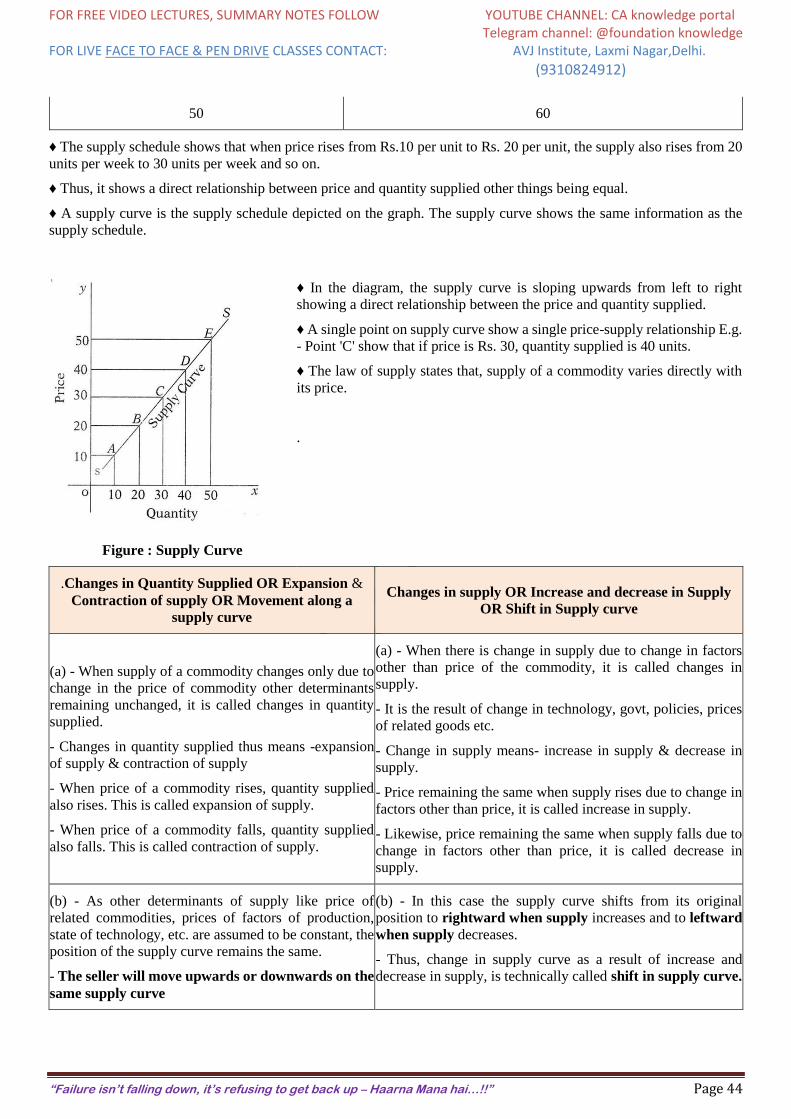
FOR FREE VIDEO LECTURES, SUMMARY NOTES FOLLOW YOUTUBE CHANNEL: CA knowledge portal Telegram channel: @foundation knowledge FOR LIVE FACE TO FACE & PEN DRIVE CLASSES CONTACT: AVJ Institute, Laxmi Nagar,Delhi.
(9310824912)
“Failure isn’t falling down, it’s refusing to get back up – Haarna Mana hai…!!” Page 44
50 60
♦ The supply schedule shows that when price rises from Rs.10 per unit to Rs. 20 per unit, the supply also rises from 20
units per week to 30 units per week and so on.
♦ Thus, it shows a direct relationship between price and quantity supplied other things being equal.
♦ A supply curve is the supply schedule depicted on the graph. The supply curve shows the same information as the
supply schedule.
♦ In the diagram, the supply curve is sloping upwards from left to right
showing a direct relationship between the price and quantity supplied.
♦ A single point on supply curve show a single price-supply relationship E.g.
- Point 'C' show that if price is Rs. 30, quantity supplied is 40 units.
♦ The law of supply states that, supply of a commodity varies directly with
its price.
.
Figure : Supply Curve
.Changes in Quantity Supplied OR Expansion &
Contraction of supply OR Movement along a
supply curve
Changes in supply OR Increase and decrease in Supply
OR Shift in Supply curve
(a) - When supply of a commodity changes only due to
change in the price of commodity other determinants
remaining unchanged, it is called changes in quantity
supplied.
- Changes in quantity supplied thus means -expansion
of supply & contraction of supply
- When price of a commodity rises, quantity supplied
also rises. This is called expansion of supply.
- When price of a commodity falls, quantity supplied
also falls. This is called contraction of supply.
(a) - When there is change in supply due to change in factors
other than price of the commodity, it is called changes in
supply.
- It is the result of change in technology, govt, policies, prices
of related goods etc.
- Change in supply means- increase in supply & decrease in
supply.
- Price remaining the same when supply rises due to change in
factors other than price, it is called increase in supply.
- Likewise, price remaining the same when supply falls due to
change in factors other than price, it is called decrease in
supply.
(b) - As other determinants of supply like price of
related commodities, prices of factors of production,
state of technology, etc. are assumed to be constant, the
position of the supply curve remains the same.
- The seller will move upwards or downwards on the
same supply curve
(b) - In this case the supply curve shifts from its original
position to rightward when supply increases and to leftward
when supply decreases.
- Thus, change in supply curve as a result of increase and
decrease in supply, is technically called shift in supply curve.
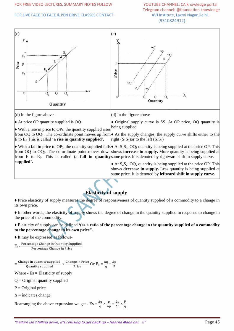
FOR FREE VIDEO LECTURES, SUMMARY NOTES FOLLOW YOUTUBE CHANNEL: CA knowledge portal Telegram channel: @foundation knowledge FOR LIVE FACE TO FACE & PEN DRIVE CLASSES CONTACT: AVJ Institute, Laxmi Nagar,Delhi.
(9310824912)
“Failure isn’t falling down, it’s refusing to get back up – Haarna Mana hai…!!” Page 45
(c)
(c)
(d) In the figure above -
♦ At price OP quantity supplied is OQ
♦ With a rise in price to OP1, the quantity supplied rises
from OQ to OQ1. The co-ordinate point moves up from
E to E1 This is called ‘a rise in quantity supplied'.
♦ With a fall in price to OP2, the quantity supplied falls
from OQ to OQ2. The co-ordinate point moves down
from E to E2. This is called (a fall in quantity
supplied’.
(d) In the figure above-
♦ Original supply curve is SS. At OP price, OQ quantity is
being supplied.
♦ As the supply changes, the supply curve shifts either to the
right (S1S1)or to the left (S2S2)
♦ At S1S1, OQ1 quantity is being supplied at the price OP. This
shows increase in supply. More quantity is being supplied at
same price. It is denoted by rightward shift in supply curve.
♦ At S2S2, OQ2 quantity is being supplied at the price OP. This
shows decrease in supply. Less quantity is being supplied at
same price. It is denoted by leftward shift in supply curve.
Elasticity of supply
♦ Price elasticity of supply measures the degree of responsiveness of quantity supplied of a commodity to a change in
its own price.
♦ In other words, the elasticity of supply shows the degree of change in the quantity supplied in response to change in
the price of the commodity.
♦ Elasticity of supply can be defined ‘(as a ratio of the percentage change in the quantity supplied of a commodity
to the percentage change in its own price".
♦ It may be expressed as follows-
Es = Percentage Change in Quantity Supplied
Percentage Change in Price
= Change in quantity supplied
Quantity supplied ÷
Change in Price
Price Or Es =
∆q
q ÷
∆p
P
Where - Es = Elasticity of supply
Q = Original quantity supplied
P = Original price
Δ = indicates change
Rearranging the above expression we get - Es = ∆q
q ×
p
Ap =
∆q
∆p ×
P
q
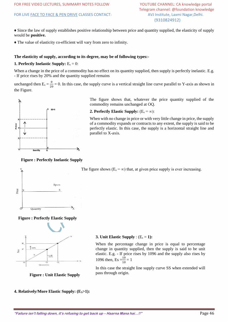
FOR FREE VIDEO LECTURES, SUMMARY NOTES FOLLOW YOUTUBE CHANNEL: CA knowledge portal Telegram channel: @foundation knowledge FOR LIVE FACE TO FACE & PEN DRIVE CLASSES CONTACT: AVJ Institute, Laxmi Nagar,Delhi.
(9310824912)
“Failure isn’t falling down, it’s refusing to get back up – Haarna Mana hai…!!” Page 46
♦ Since the law of supply establishes positive relationship between price and quantity supplied, the elasticity of supply
would be positive.
♦ The value of elasticity co-efficient will vary from zero to infinity.
The elasticity of supply, according to its degree, may be of following types:-
1. Perfectly Inelastic Supply: Es = 0:
When a change in the price of a commodity has no effect on its quantity supplied, then supply is perfectly inelastic. E.g.
- If price rises by 20% and the quantity supplied remains
unchanged then Es = 0
20 = 0. In this case, the supply curve is a vertical straight line curve parallel to Y-axis as shown in
the Figure.
The figure shows that, whatever the price quantity supplied of the
commodity remains unchanged at OQ.
2. Perfectly Elastic Supply: (Es = ∞):
When with no change in price or with very little change in price, the supply
of a commodity expands or contracts to any extent, the supply is said to be
perfectly elastic. In this case, the supply is a horizontal straight line and
parallel to X-axis.
Figure : Perfectly Inelastic Supply
The figure shows (Es = ∞) that, at given price supply is ever increasing.
Figure : Perfectly Elastic Supply
3. Unit Elastic Supply : (Es = 1):
When the percentage change in price is equal to percentage
change in quantity supplied, then the supply is said to be unit
elastic. E.g. - If price rises by 1096 and the supply also rises by
1096 then, Es =10
10 = 1
In this case the straight line supply curve SS when extended will
pass through origin. Figure : Unit Elastic Supply
4. Relatively/More Elastic Supply: (ES>1):
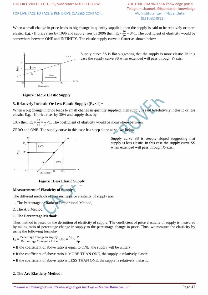
FOR FREE VIDEO LECTURES, SUMMARY NOTES FOLLOW YOUTUBE CHANNEL: CA knowledge portal Telegram channel: @foundation knowledge FOR LIVE FACE TO FACE & PEN DRIVE CLASSES CONTACT: AVJ Institute, Laxmi Nagar,Delhi.
(9310824912)
“Failure isn’t falling down, it’s refusing to get back up – Haarna Mana hai…!!” Page 47
When a small change in price leads to big change in quantity supplied, then the supply is said to be relatively or more
elastic. E.g. - If price rises by 1096 and supply rises by 3096 then, Es = 30
10 = 3>1. The coefficient of elasticity would be
somewhere between ONE and INFINITY. The elastic supply curve is flatter as shown below-
Supply curve SS is flat suggesting that the supply is more elastic. In this
case the supply curve SS when extended will pass through Y-axis.
Figure : More Elastic Supply
5. Relatively Inelastic Or Less Elastic Supply: (ES <1) •
When a big change in price leads to small change in quantity supplied, then supply is said to relatively inelastic or less
elastic. E.g. - If price rises by 30% and supply rises by
10% then, Es = 10
30 =
1
3 <1. The coefficient of elasticity would be somewhere between
ZERO and ONE. The supply curve in this case has steep slope as shown below –
Supply curve SS is steeply sloped suggesting that
supply is less elastic. In this case the supply curve SS
when extended will pass through X-axis.
Figure : Less Elastic Supply
Measurement of Elasticity of Supply.
The different methods of measuring price elasticity of supply are:
1. The Percentage or Ratio or Proportional Method,
2. The Arc Method
1. The Percentage Method:
Thus method is based on the definition of elasticity of supply. The coefficient of price elasticity of supply is measured
by taking ratio of percentage change in supply to the percentage change in price. Thus, we measure the elasticity by
using the following formula-
Es = Pecentage Change in Supply
Percentage Change in Price OR =
∆q
q ×
P
∆p
♦ If the coefficient of above ratio is equal to ONE, the supply will be unitary.
♦ If the coefficient of above ratio is MORE THAN ONE, the supply is relatively elastic.
♦ If the coefficient of above ratio is LESS THAN ONE, the supply is relatively inelastic.
2. The Arc Elasticity Method:
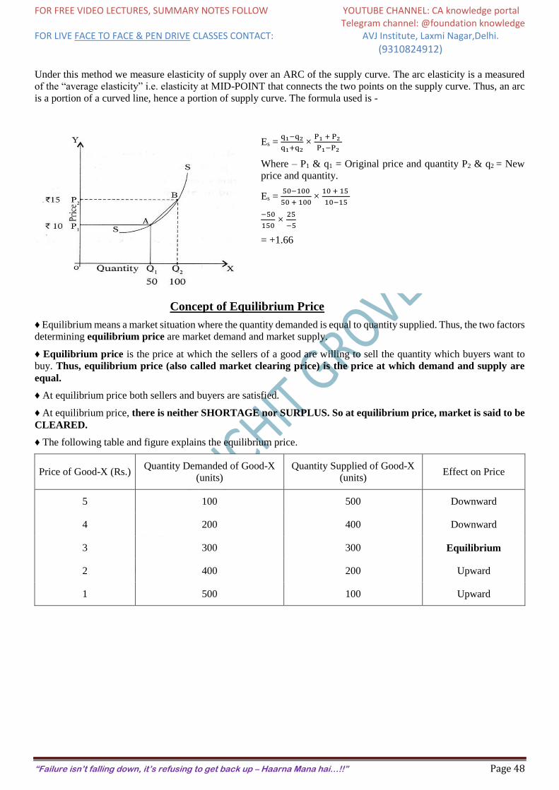
FOR FREE VIDEO LECTURES, SUMMARY NOTES FOLLOW YOUTUBE CHANNEL: CA knowledge portal Telegram channel: @foundation knowledge FOR LIVE FACE TO FACE & PEN DRIVE CLASSES CONTACT: AVJ Institute, Laxmi Nagar,Delhi.
(9310824912)
“Failure isn’t falling down, it’s refusing to get back up – Haarna Mana hai…!!” Page 48
Under this method we measure elasticity of supply over an ARC of the supply curve. The arc elasticity is a measured
of the “average elasticity” i.e. elasticity at MID-POINT that connects the two points on the supply curve. Thus, an arc
is a portion of a curved line, hence a portion of supply curve. The formula used is -
Es = q1−q2
q1+q2 ×
P1 + P2
P1−P2
Where – P1 & q1 = Original price and quantity P2 & q2 = New
price and quantity.
Es = 50−100
50 + 100 ×
10 + 15
10−15
−50
150 ×
25
−5
= +1.66
Concept of Equilibrium Price
♦ Equilibrium means a market situation where the quantity demanded is equal to quantity supplied. Thus, the two factors
determining equilibrium price are market demand and market supply.
♦ Equilibrium price is the price at which the sellers of a good are willing to sell the quantity which buyers want to
buy. Thus, equilibrium price (also called market clearing price) is the price at which demand and supply are
equal.
♦ At equilibrium price both sellers and buyers are satisfied.
♦ At equilibrium price, there is neither SHORTAGE nor SURPLUS. So at equilibrium price, market is said to be
CLEARED.
♦ The following table and figure explains the equilibrium price.
Price of Good-X (Rs.) Quantity Demanded of Good-X
(units)
Quantity Supplied of Good-X
(units) Effect on Price
5 100 500 Downward
4 200 400 Downward
3 300 300 Equilibrium
2 400 200 Upward
1 500 100 Upward
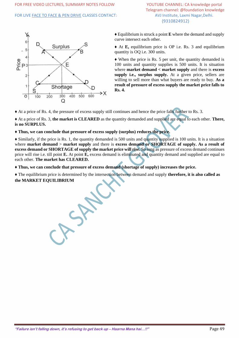
FOR FREE VIDEO LECTURES, SUMMARY NOTES FOLLOW YOUTUBE CHANNEL: CA knowledge portal Telegram channel: @foundation knowledge FOR LIVE FACE TO FACE & PEN DRIVE CLASSES CONTACT: AVJ Institute, Laxmi Nagar,Delhi.
(9310824912)
“Failure isn’t falling down, it’s refusing to get back up – Haarna Mana hai…!!” Page 49
♦ Equilibrium is struck a point E where the demand and supply
curve intersect each other.
♦ At E, equilibrium price is OP i.e. Rs. 3 and equilibrium
quantity is OQ i.e. 300 units.
♦ When the price is Rs. 5 per unit, the quantity demanded is
100 units and quantity supplies is 500 units. It is situation
where market demand < market supply and there is excess
supply i.e., surplus supply. At a given price, sellers are
willing to sell more than what buyers are ready to buy. As a
result of pressure of excess supply the market price falls to
Rs. 4.
♦ At a price of Rs. 4, the pressure of excess supply still continues and hence the price falls further to Rs. 3.
♦ At a price of Rs. 3, the market is CLEARED as the quantity demanded and supplied are equal to each other. There,
is no SURPLUS.
♦ Thus, we can conclude that pressure of excess supply (surplus) reduces the price.
♦ Similarly, if the price is Rs. 1, the quantity demanded is 500 units and quantity supplied is 100 units. It is a situation
where market demand > market supply and there is excess demand or SHORTAGE of supply. As a result of
excess demand or SHORTAGE of supply the market price will rise. So long as pressure of excess demand continues
price will rise i.e. till point E. At point E, excess demand is eliminated and quantity demand and supplied are equal to
each other. The market has CLEARED.
♦ Thus, we can conclude that pressure of excess demand (shortage of supply) increases the price.
♦ The equilibrium price is determined by the intersection between demand and supply therefore, it is also called as
the MARKET EQUILIBRIUM
FOR FREE VIDEO LECTURES, SUMMARY NOTES FOLLOW YOUTUBE CHANNEL: CA knowledge portal Telegram channel: @foundation knowledge FOR LIVE FACE TO FACE & PEN DRIVE CLASSES CONTACT: AVJ Institute, Laxmi Nagar,Delhi.
(9310824912)
“Failure isn’t falling down, it’s refusing to get back up – Haarna Mana hai…!!” Page 50

9310824912/9310824712/011-42576010
Telegram:- CA FOUNDATION KNOWLEDGE PORTAL
Youtube:- CA KNOWLEDGE PORTAL
CA FOUNDATION
Be Assured of more than 80 Marks in
Bus. Economics
&
Bus. Commercial Knowledge
CA SANCHIT GROVER
Economics 2500/- Bus. Commercial Knowledge 1500/-
COMBO- 3500/- & GOOGLE DRIVE 3000/-
AVJINSTITUTE....always ahead CA INTER/FINAL
FOUNDATION
AVJ
CA SAHIL GROVER
Pen Drive Classes
CA-INTER
Pen Drive Classes
GSTfor Nov.18 & May.19
CA SANCHIT GROVER(Senior tax consultant with Big 4 firm)
@ 4500/-
@ 4000/-
50 hours 2.5 views 93108249129310824712C
all
50%
Off for Nov.18 Exam