Kobe I (Kobe plot) +Kobe II (risk assessment) software Material/Stock... · IOTC–2014–WPTT16–53(revised) (Jan. 15, 2015) 4 2 Installation 1) Uninstall the old versions of Kobe

IOTC–2014–WPTT16–53(revised) (Jan. 15, 2015)

1

Trainingmaterials(07)TrainingcourseonstockassessmentsofLongtailtunaandKawakawaintheSEAsia

SEAFDEC/MFRDMD,KualaTerengganu,Malaysia(April17-25,2016)

Kobe I (Kobe plot) +Kobe II (risk assessment) software (New version 3, 2014)

User’s manual

Tom NISHIDA1/, Toshihide KITAKADO2/, Kazuharu IWASAKI3/ and Kiyoshi ITOH3/

1/ Corresponding author ([email protected]) National Research Institute of Far Seas Fisheries (NRIFSF),

Fisheries Research Agency (FRA), Shimizu, Shizuoka, Japan 2/ Tokyo University of Marine Science and Technology, Tokyo, Tokyo, Japan 3/ Environmental Simulation Laboratory (ESL) Inc., Kawagoe, Saitama, Japan

Abstract and Notice (release of the software)

This is the users’ manual describing how to use the 3rd version of Kobe I (stock status trajectory plots) +Kobe II (risk assessment diagram) software. Kobe I and II were recommended by the 5 tuna-RFMO meeting in 2007 (Kobe, Japan) and 2009 (Barcelona, Spain) respectively. This software is free of charge available at http://ocean-info.ddo.jp/kobeaspm/kobeplot/KobePlot.zip (from Nov. 19, 2014). After users use this software and if users need improvements, please let us know. We will revise and will release more user’s friendly software. As for Kobe II, the risk assessment matrix format was recommended, but the table formats have been difficult to understand its meanings often, especially for mangers and industries as it uses mathematical and technical notations. To improve this situation, we developed the visualized presentation (diagram) of the matrix for anyone to be able to understand its meanings easily. Please note that this software is suitable for those who have difficulties to make Kobe I plot and II quickly and effectively in a very short time, especially during the working meetings. Thus it may not be suitable for those who can make these plots and diagrams and/or create better ones by own using specific codes such as R. This is because this software can make fixed designed plots and diagrams. However, it has a lot of flexibilities to change colors, fonts, lines, symbols, legends and labels by graph setting functions (see the text for details). This software development project has been funded by Fisheries Agency of Japan (2009-2014) for Tuna and Skipjack Resources Division, National Research Institute of Far Seas Fisheries (NRIFSF), Fisheries Research Agency of Japan (FRA). We sincerely acknowledge their continuous financial supports for this project.

Contents Acronyms--------------------------------------------------------------------------------------------------- 02 1. Introduction------------------------------------------------------------------------------------------- 03 2. Installation-------------------------------------------------------------------------------------------- 04-06 3. Starting software------------------------------------------------------------------------------------- 07-08 4. Kobe Plot I (stock status trajectory) (3 options)

4.1 Option 1: A single plot with a confidence surface----------------------------------------- 09-15 4.2 Option 2: Multiple plots without confidence surface------------------------------------- 15-19 4.3 Option 3: Multiple comparisons among different stock assessment results---------- 20-22 4.4 Common functions (editing, moving labels and saving)--------------------------------- 22-28

5. Kobe Plot II (risk assessment diagram) ---------------------------------------------------------- 29-34 Acknowledgements---------------------------------------------------------------------------------------- 34 References-------------------------------------------------------------------------------------------------- 35 Appendix A: Software specification-------------------------------------------------------------------- 35 _______________________________________________________ Submitted to the IOTC WPTT16 (November 15-19, 2014), Bali, Indonesia.


2

ACRONYMS

B Total biomass

BBDM Bayesian Biomass Dynamics Model

Bmsy Biomass which produces MSY

CI Confidence interval

F Fishing mortality; F2010 is the fishing mortality estimated in the year 2010

Fmsy Fishing mortality at MSY

IOTC Indian Ocean Tuna Commission

LRP Limit Reference Point

MFCL Multifan-CL

MSY Maximum Sustainable Yield

SB Spawning biomass (sometimes expressed as SSB)

SBmsy Spawning stock biomass which produces MSY

TRP Target Reference Point


3

1. Introduction 1.1 Overview This Kobe I+II software consists of Kobe I (stock status trajectory plot) and Kobe II (risk assessment diagram). Kobe Plot I can make historical stock status trajectory plots for SB/SBmsy (or B/Bmsy) and F/Fmsy using results of stock assessments. Kobe II depicts color diagrams for results of risk assessments for SB/SBmsy and F/Fmsy, i.e., probabilities violating their MSY levels in the future by different catch level scenarios.

1.2 Operation Systems (OS) This software can be used under MS windows OS operated by both 32 and 64-bit PCs. 1.3 History of the development 1st version (2011) (IOTC-2011-WPTT13-45) l Release of the initial Kobe plot software containing basic functions for Kobe I plot and

Kobe II diagram. 2nd version (2012) (IOTC-2012-WPM04-05) l Graphic components were improved using TeeChart Pro.NET v2010 (Steema

Software) according to requests by worldwide users. l Release of two separate software for 32- and 64-bit OS PCs. 3rd version (2014) (IOTC-2014-WPTT16-53) l Release of one united software for both 32- and 64-bit OS PCs for window OS. l Designs and functions of Kobe plot I are further improved according to requests by

worldwide users. l Limit and target reference points can be depicted. l One menu in Kobe I plot is added to show multiple comparisons among different stock

assessment results. l Pie chart option is added in Kobe Plot to show compositions of uncertainties in 4

phases.


4

2 Installation

1) Uninstall the old versions of Kobe I+II software if users have.

If users installed the previous versions, uninstall it first.

2) Download the package (Version 3, 2014) including software, manual and other

references from http://ocean-info.ddo.jp/kobeaspm/kobeplot/KobePlot.zip.

You will get

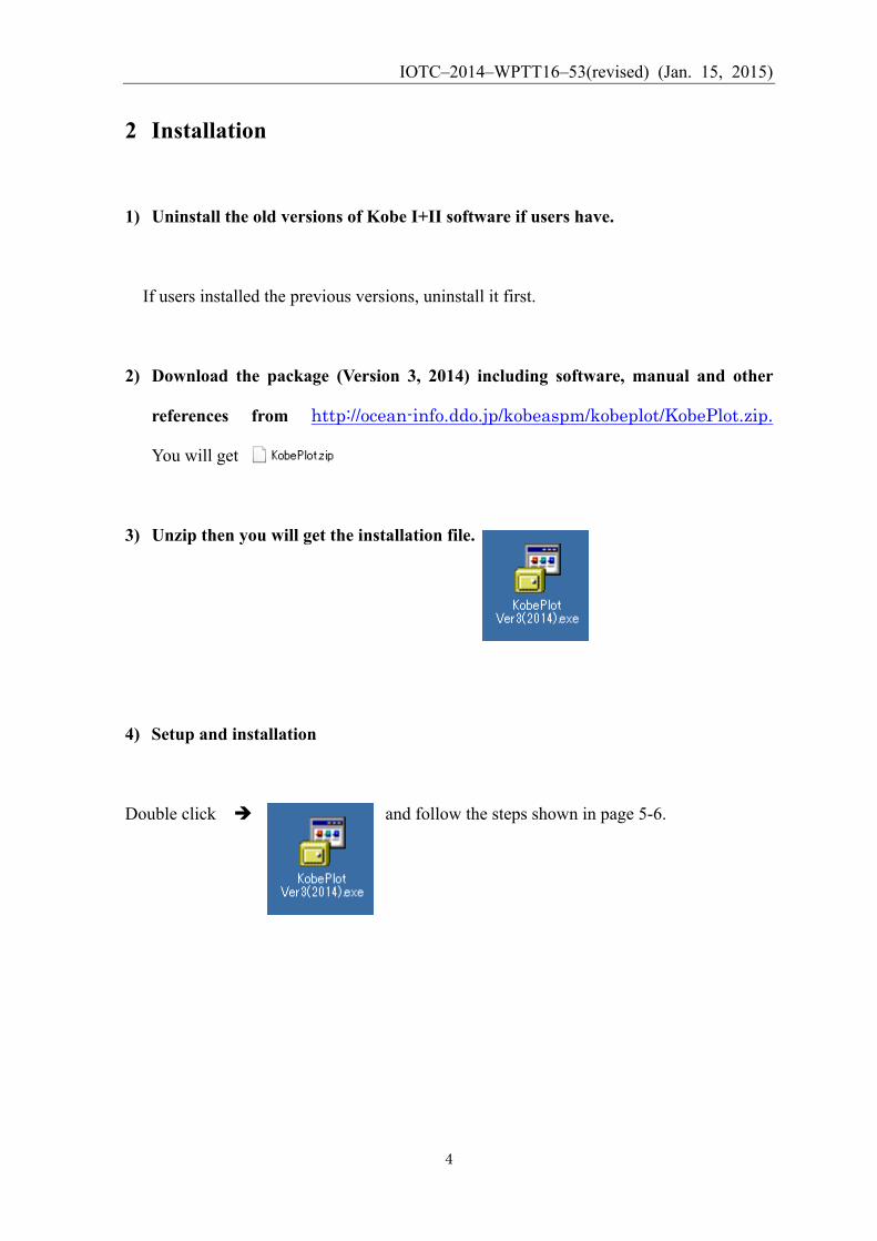
3) Unzip then you will get the installation file.

4) Setup and installation

Double click è and follow the steps shown in page 5-6.


5

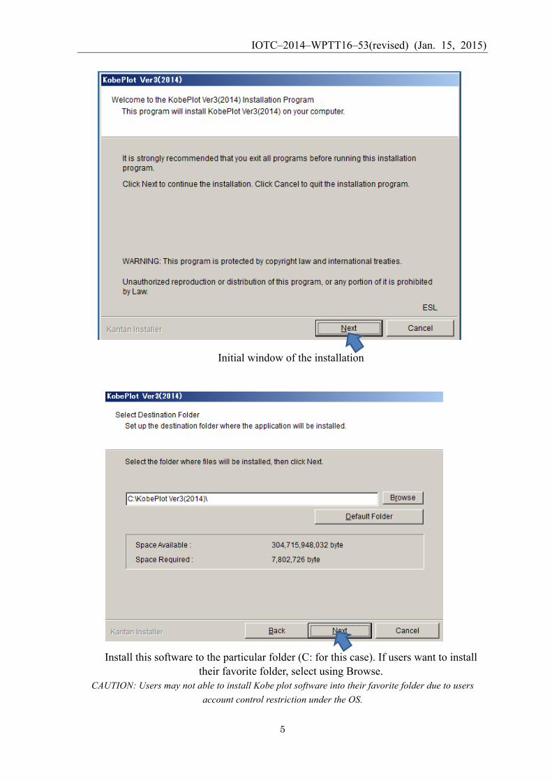
Initial window of the installation

Install this software to the particular folder (C: for this case). If users want to install

their favorite folder, select using Browse. CAUTION: Users may not able to install Kobe plot software into their favorite folder due to users

account control restriction under the OS.


6

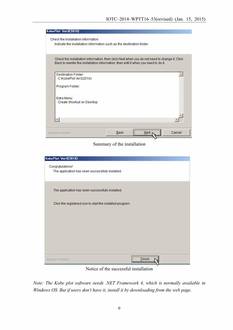
Summary of the installation

Notice of the successful installation

Note: The Kobe plot software needs .NET Framework 4, which is normally available in Windows OS. But if users don’t have it, install it by downloading from the web page.


7

3. Starting the software

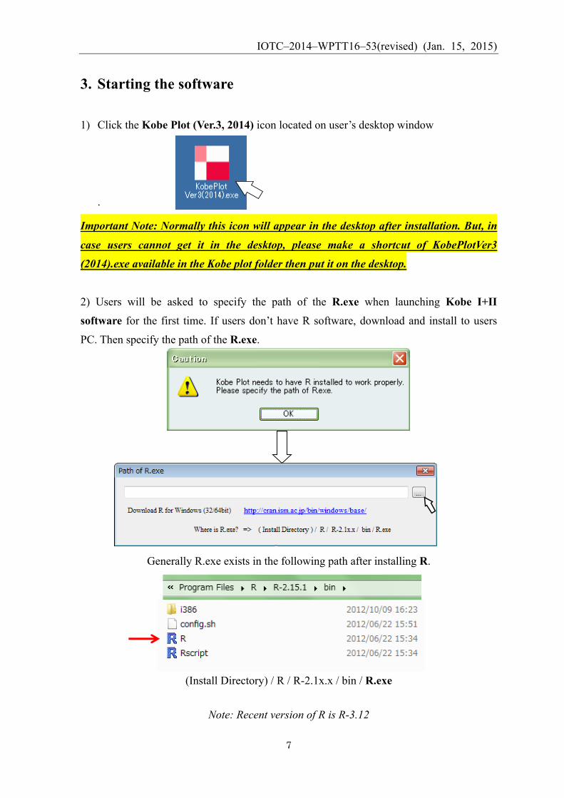
1) Click the Kobe Plot (Ver.3, 2014) icon located on user’s desktop window

.

Important Note: Normally this icon will appear in the desktop after installation. But, in

case users cannot get it in the desktop, please make a shortcut of KobePlotVer3

(2014).exe available in the Kobe plot folder then put it on the desktop.

2) Users will be asked to specify the path of the R.exe when launching Kobe I+II

software for the first time. If users don’t have R software, download and install to users

PC. Then specify the path of the R.exe.

Generally R.exe exists in the following path after installing R.

(Install Directory) / R / R-2.1x.x / bin / R.exe

Note: Recent version of R is R-3.12


8

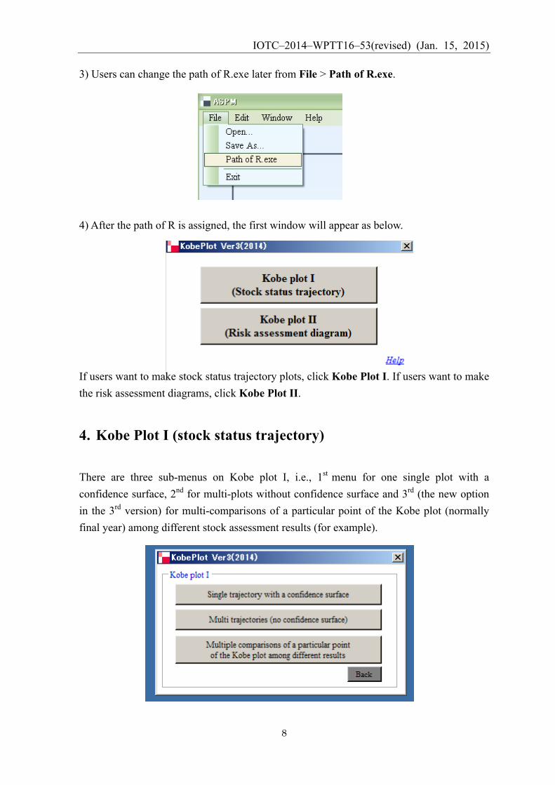
3) Users can change the path of R.exe later from File > Path of R.exe.

4) After the path of R is assigned, the first window will appear as below.

If users want to make stock status trajectory plots, click Kobe Plot I. If users want to make the risk assessment diagrams, click Kobe Plot II.

4. Kobe Plot I (stock status trajectory)

There are three sub-menus on Kobe plot I, i.e., 1st menu for one single plot with a confidence surface, 2nd for multi-plots without confidence surface and 3rd (the new option in the 3rd version) for multi-comparisons of a particular point of the Kobe plot (normally final year) among different stock assessment results (for example).


9

4.1 A single plot with a confidence surface

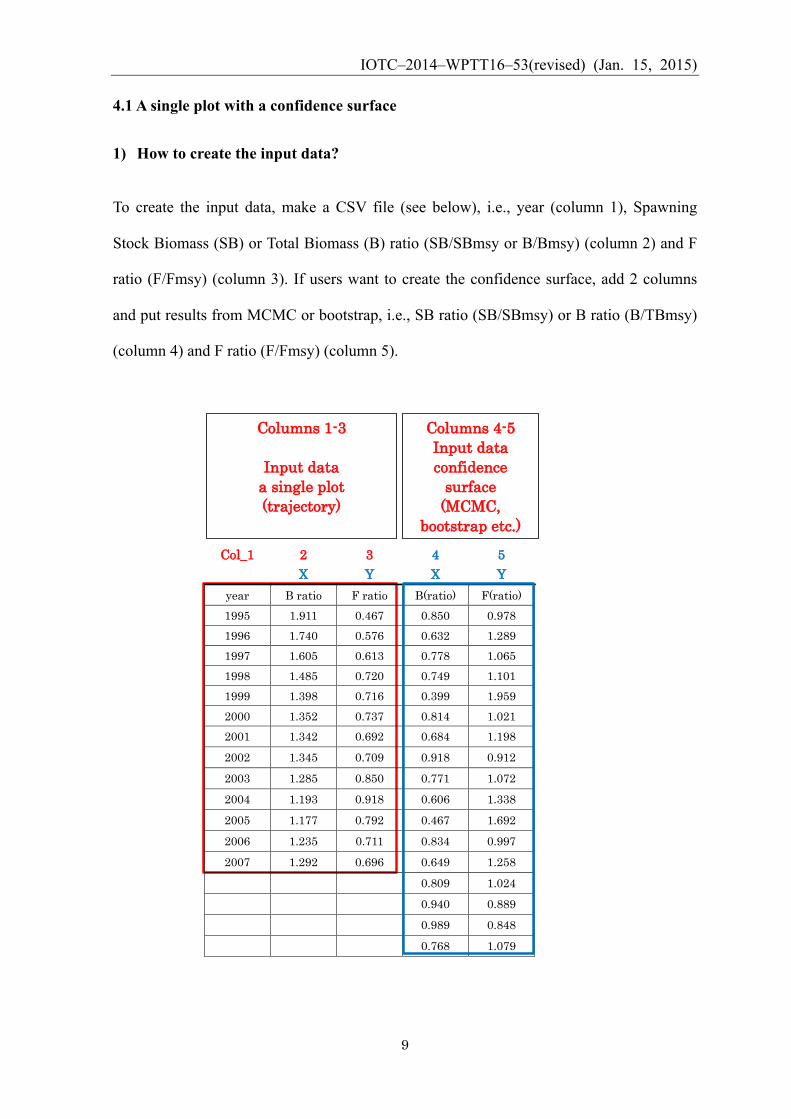
1) How to create the input data?

To create the input data, make a CSV file (see below), i.e., year (column 1), Spawning

Stock Biomass (SB) or Total Biomass (B) ratio (SB/SBmsy or B/Bmsy) (column 2) and F

ratio (F/Fmsy) (column 3). If users want to create the confidence surface, add 2 columns

and put results from MCMC or bootstrap, i.e., SB ratio (SB/SBmsy) or B ratio (B/TBmsy)

(column 4) and F ratio (F/Fmsy) (column 5).

Col_1 2 3 4 5 X Y X Y

year B ratio F ratio B(ratio) F(ratio) 1995 1.911 0.467 0.850 0.978 1996 1.740 0.576 0.632 1.289 1997 1.605 0.613 0.778 1.065 1998 1.485 0.720 0.749 1.101 1999 1.398 0.716 0.399 1.959 2000 1.352 0.737 0.814 1.021 2001 1.342 0.692 0.684 1.198 2002 1.345 0.709 0.918 0.912 2003 1.285 0.850 0.771 1.072 2004 1.193 0.918 0.606 1.338 2005 1.177 0.792 0.467 1.692 2006 1.235 0.711 0.834 0.997 2007 1.292 0.696 0.649 1.258

0.809 1.024 0.940 0.889 0.989 0.848 0.768 1.079

Columns 4-5 Input data confidence

surface (MCMC,

bootstrap etc.)

Columns 1-3

Input data a single plot (trajectory)


10

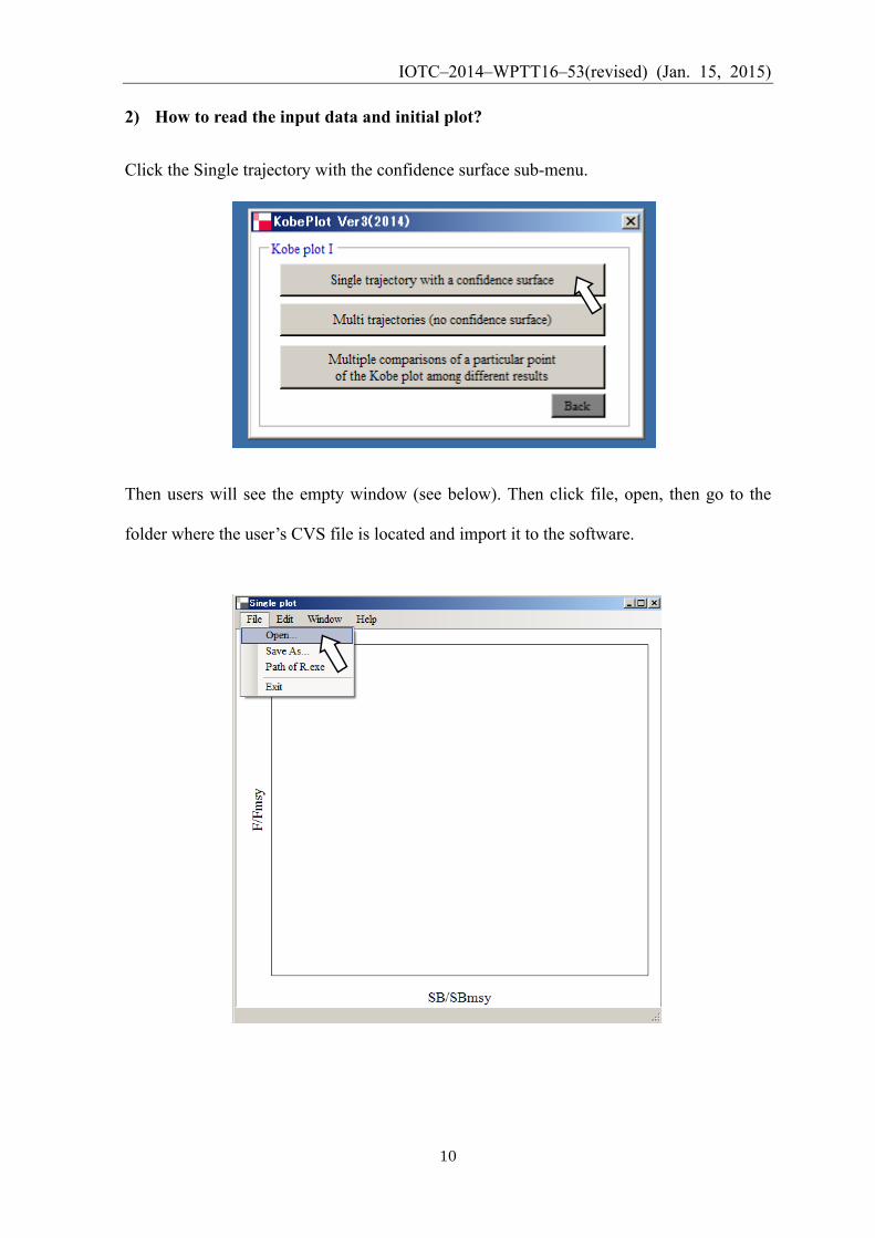
2) How to read the input data and initial plot? Click the Single trajectory with the confidence surface sub-menu.

Then users will see the empty window (see below). Then click file, open, then go to the

folder where the user’s CVS file is located and import it to the software.


11

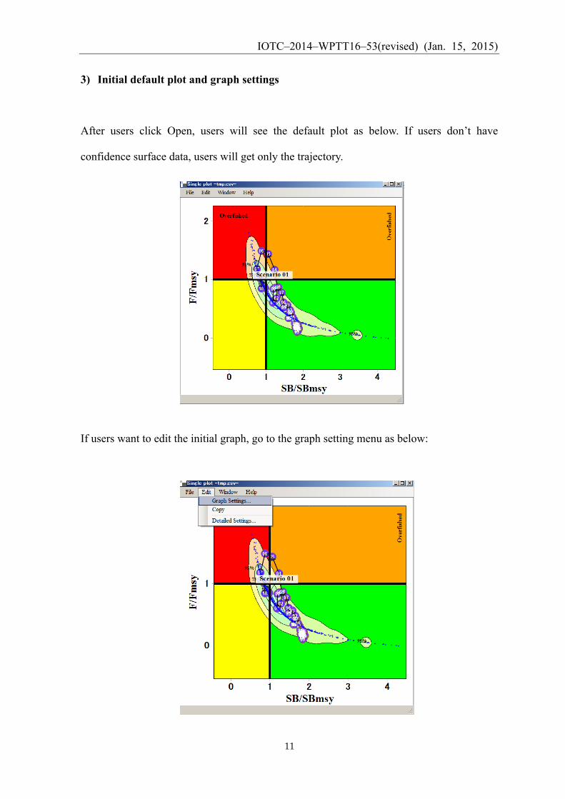
3) Initial default plot and graph settings

After users click Open, users will see the default plot as below. If users don’t have

confidence surface data, users will get only the trajectory.

If users want to edit the initial graph, go to the graph setting menu as below:


12

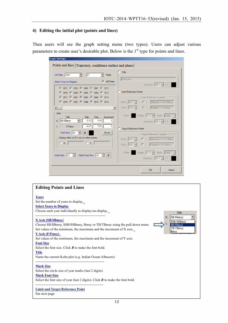
4) Editing the initial plot (points and lines) Then users will see the graph setting menu (two types). Users can adjust various parameters to create user’s desirable plot. Below is the 1st type for points and lines.

Editing Points and Lines Years Set the number of years to display. Select Years to Display Choose each year individually to display/un-display. ------------------------------------------------------------- X Axis (SB/SBmsy) Choose SB/SBmsy, SSB/SSBmsy, Bmsy or TB/TBmsy using the pull down menu. Set values of the minimum, the maximum and the increment of X axis. Y Axis (F/Fmsy) Set values of the minimum, the maximum and the increment of Y axis. Font Size Select the font size. Click B to make the font bold. Title Name the current Kobe plot (e.g. Indian Ocean Albacore) ------------------------------------------------------------ Mark Size Select the circle size of year marks (last 2 digits). Mark Font Size Select the font size of year (last 2 digits). Click B to make the font bold. ----------------------------------------------------------- Limit and Target Reference Point See next page


13

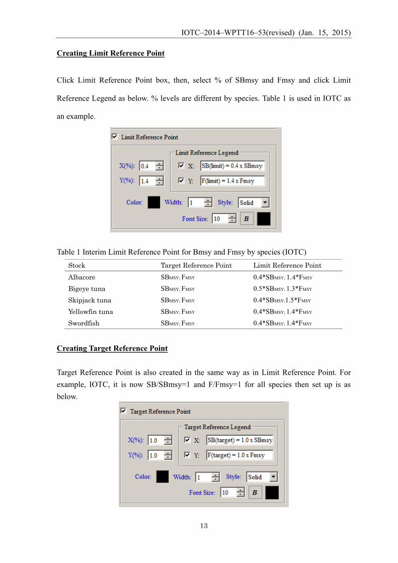
Creating Limit Reference Point

Click Limit Reference Point box, then, select % of SBmsy and Fmsy and click Limit

Reference Legend as below. % levels are different by species. Table 1 is used in IOTC as

an example.

Table 1 Interim Limit Reference Point for Bmsy and Fmsy by species (IOTC)

Creating Target Reference Point Target Reference Point is also created in the same way as in Limit Reference Point. For example, IOTC, it is now SB/SBmsy=1 and F/Fmsy=1 for all species then set up is as below.

Stock Target Reference Point Limit Reference Point Albacore SBMSY; FMSY 0.4*SBMSY; 1.4*FMSY Bigeye tuna SBMSY; FMSY 0.5*SBMSY; 1.3*FMSY Skipjack tuna SBMSY; FMSY 0.4*SBMSY;1.5*FMSY Yellowfin tuna SBMSY; FMSY 0.4*SBMSY; 1.4*FMSY Swordfish SBMSY; FMSY 0.4*SBMSY; 1.4*FMSY


14

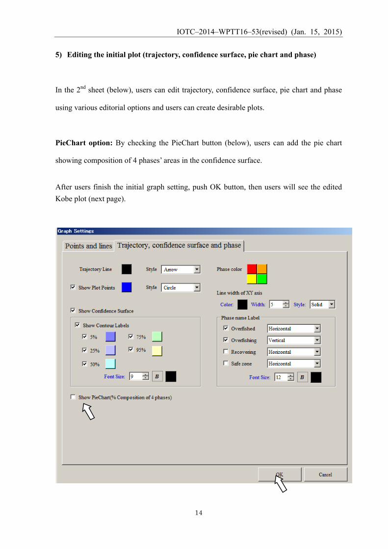
5) Editing the initial plot (trajectory, confidence surface, pie chart and phase)

In the 2nd sheet (below), users can edit trajectory, confidence surface, pie chart and phase

using various editorial options and users can create desirable plots.

PieChart option: By checking the PieChart button (below), users can add the pie chart

showing composition of 4 phases’ areas in the confidence surface.

After users finish the initial graph setting, push OK button, then users will see the edited Kobe plot (next page).


15

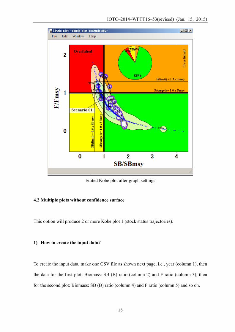
Edited Kobe plot after graph settings

4.2 Multiple plots without confidence surface

This option will produce 2 or more Kobe plot 1 (stock status trajectories).


To create the input data, make one CSV file as shown next page, i.e., year (column 1), then

the data for the first plot: Biomass: SB (B) ratio (column 2) and F ratio (column 3), then

for the second plot: Biomass: SB (B) ratio (column 4) and F ratio (column 5) and so on.


16

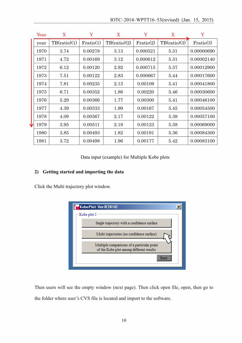
Year X Y X Y X Y year TB(ratio)(1) Fratio(1) TB(ratio)(2) Fratio(2) TB(ratio)(3) Fratio(3) 1970 3.74 0.00278 3.13 0.000521 5.31 0.00000690 1971 4.72 0.00169 3.12 0.000612 5.31 0.00002140 1972 6.12 0.00120 2.92 0.000715 5.37 0.00012900 1973 7.51 0.00122 2.83 0.000667 5.44 0.00017600 1974 7.81 0.00235 2.13 0.00109 5.41 0.00041800 1975 6.71 0.00352 1.86 0.00220 5.46 0.00030600 1976 5.29 0.00366 1.77 0.00300 5.41 0.00046100 1977 4.39 0.00333 1.99 0.00167 5.45 0.00054500 1978 4.09 0.00367 2.17 0.00122 5.39 0.00057100 1979 3.95 0.00511 2.19 0.00123 5.38 0.00069000 1980 3.85 0.00493 1.82 0.00191 5.36 0.00084300 1981 3.72 0.00498 1.96 0.00177 5.42 0.00083100

Data input (example) for Multiple Kobe plots

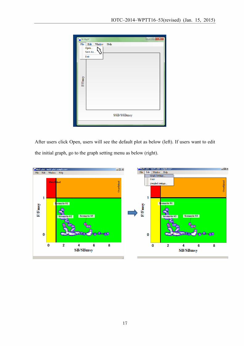
2) Getting started and importing the data Click the Multi trajectory plot window.

Then users will see the empty window (next page). Then click open file, open, then go to

the folder where user’s CVS file is located and import to the software.


17

After users click Open, users will see the default plot as below (left). If users want to edit

the initial graph, go to the graph setting menu as below (right).


18

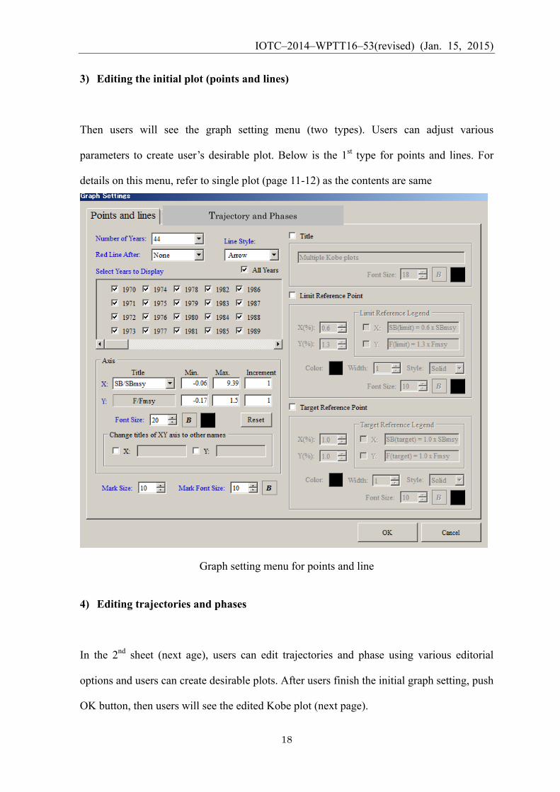
3) Editing the initial plot (points and lines)

Then users will see the graph setting menu (two types). Users can adjust various

parameters to create user’s desirable plot. Below is the 1st type for points and lines. For

details on this menu, refer to single plot (page 11-12) as the contents are same

Graph setting menu for points and line

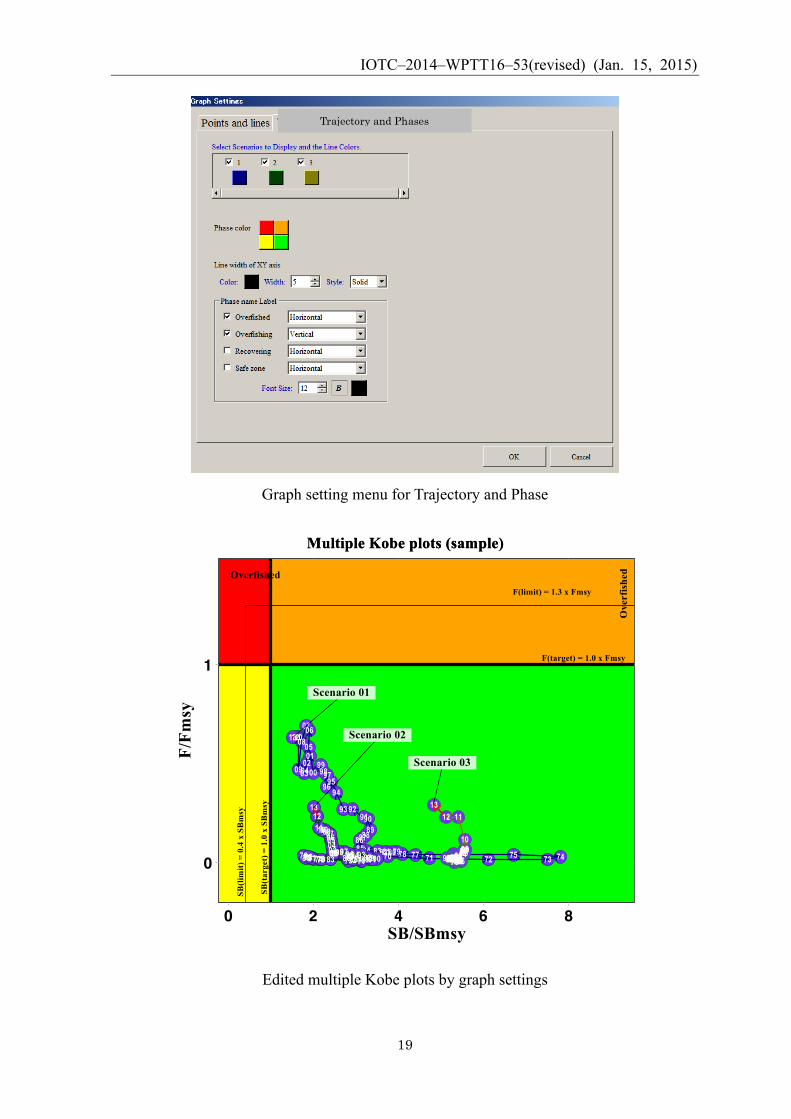
4) Editing trajectories and phases

In the 2nd sheet (next age), users can edit trajectories and phase using various editorial

options and users can create desirable plots. After users finish the initial graph setting, push

OK button, then users will see the edited Kobe plot (next page).

Trajectory and Phases


19

Graph setting menu for Trajectory and Phase

Edited multiple Kobe plots by graph settings

Trajectory and Phases


20

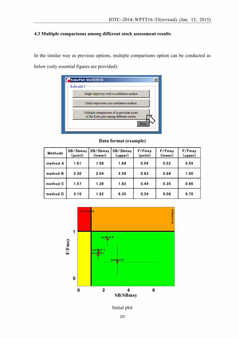
4.3 Multiple comparisons among different stock assessment results

In the similar way as previous options, multiple comparisons option can be conducted as

below (only essential figures are provided):

Data format (example)

Initial plot

MethodsSB/Sbmsy

(point)SB/Sbmsy

(lower)SB/Sbmsy

(upper)F/Fmsy(point)

F/Fmsy(lower)

F/Fmsy(upper)

method A 1.61 1.58 1.68 0.56 0.52 0.59

method B 2.30 2.04 2.56 0.83 0.68 1.00

method C 1.57 1.36 1.82 0.49 0.35 0.66

method D 3.10 1.92 6.35 0.34 0.08 0.70


21

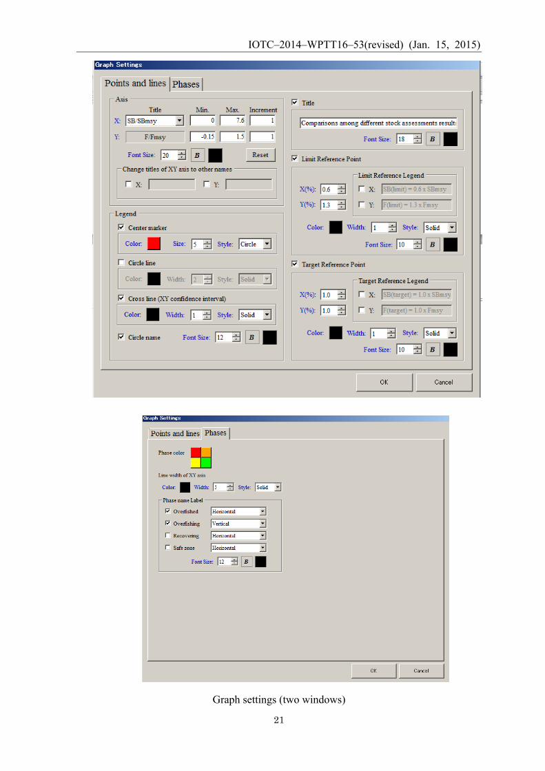
Graph settings (two windows)


22

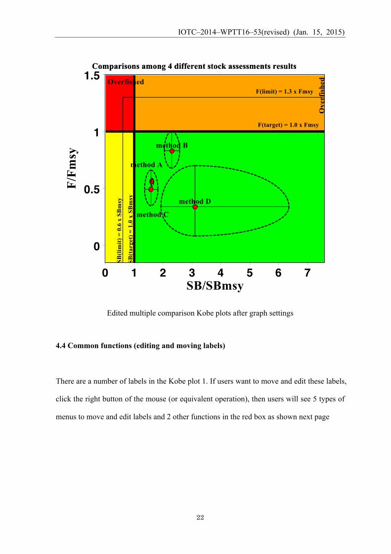
Edited multiple comparison Kobe plots after graph settings

4.4 Common functions (editing and moving labels)

There are a number of labels in the Kobe plot 1. If users want to move and edit these labels,

click the right button of the mouse (or equivalent operation), then users will see 5 types of

menus to move and edit labels and 2 other functions in the red box as shown next page


23

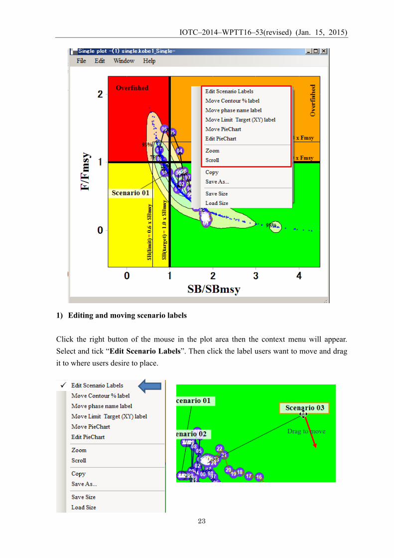
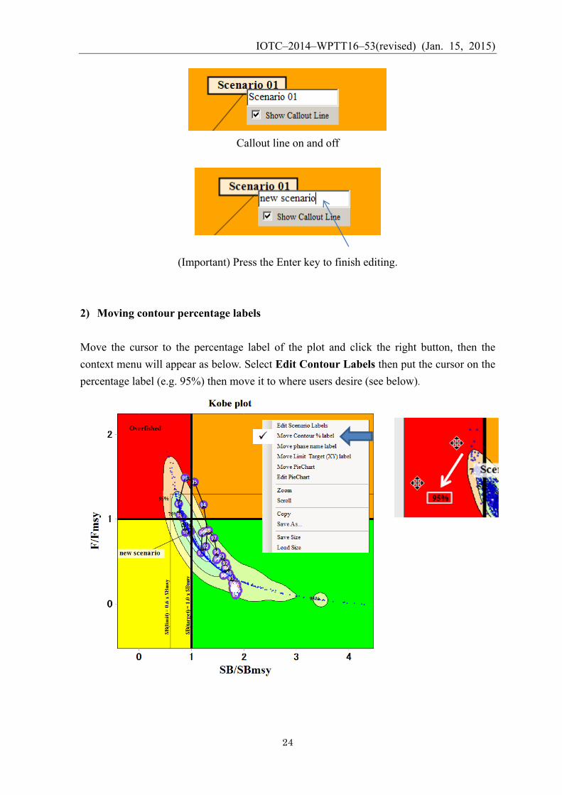
1) Editing and moving scenario labels Click the right button of the mouse in the plot area then the context menu will appear. Select and tick “Edit Scenario Labels”. Then click the label users want to move and drag it to where users desire to place.

Drag to move


24

Callout line on and off

(Important) Press the Enter key to finish editing. 2) Moving contour percentage labels Move the cursor to the percentage label of the plot and click the right button, then the context menu will appear as below. Select Edit Contour Labels then put the cursor on the percentage label (e.g. 95%) then move it to where users desire (see below).


25

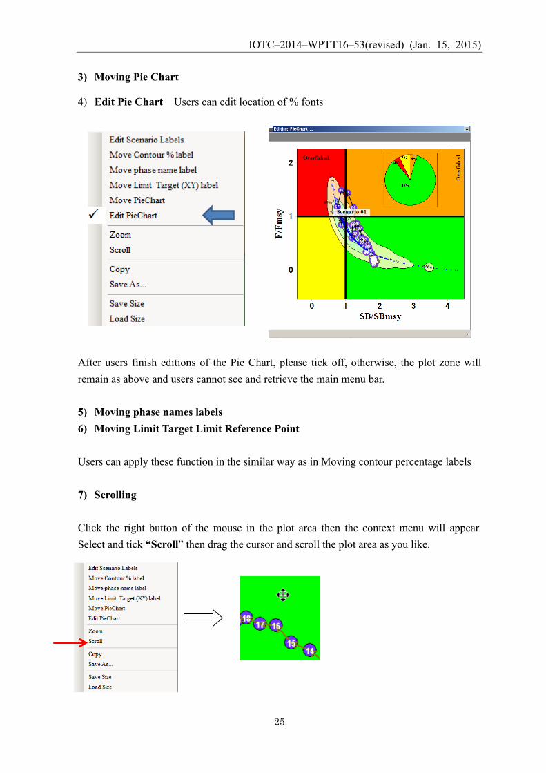
3) Moving Pie Chart

4) Edit Pie Chart Users can edit location of % fonts

After users finish editions of the Pie Chart, please tick off, otherwise, the plot zone will remain as above and users cannot see and retrieve the main menu bar.

5) Moving phase names labels 6) Moving Limit Target Limit Reference Point Users can apply these function in the similar way as in Moving contour percentage labels

7) Scrolling Click the right button of the mouse in the plot area then the context menu will appear. Select and tick “Scroll” then drag the cursor and scroll the plot area as you like.


26

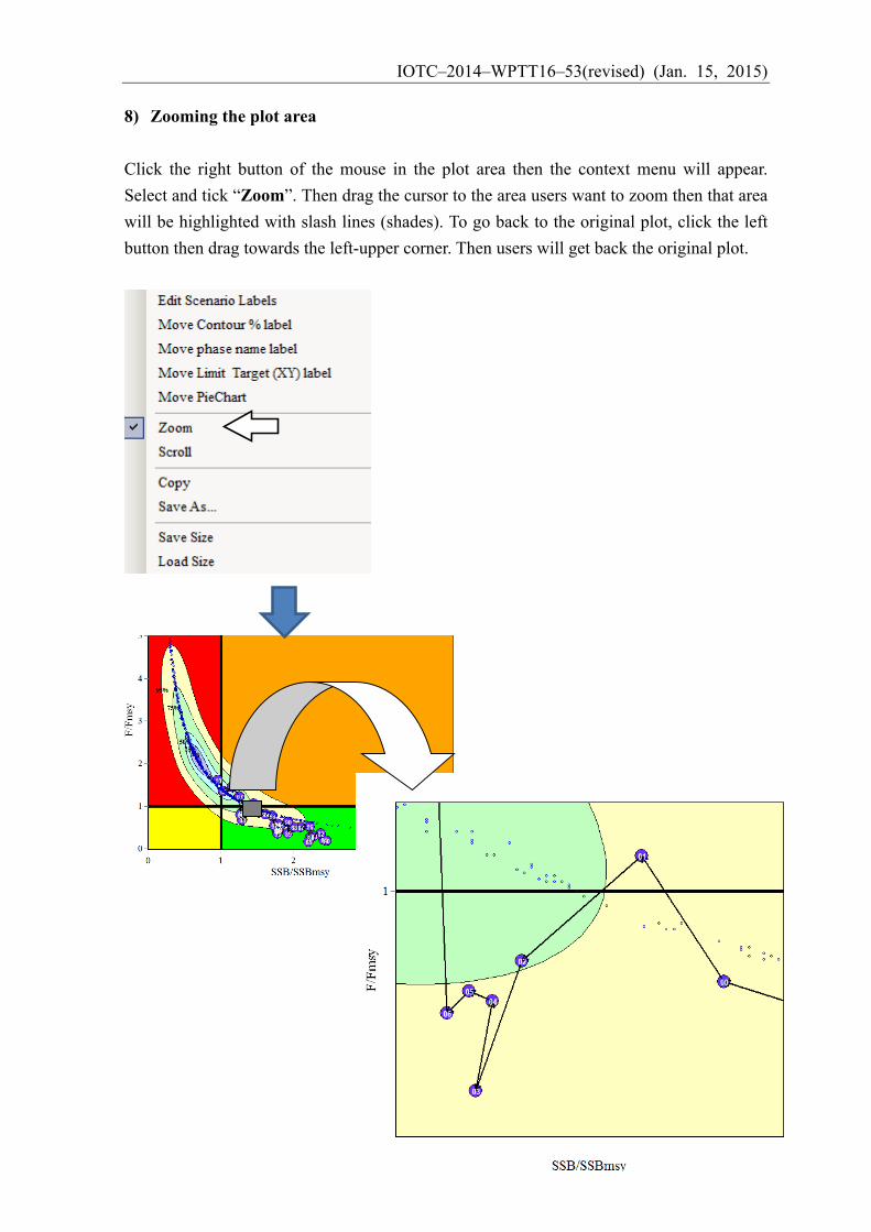
8) Zooming the plot area

Click the right button of the mouse in the plot area then the context menu will appear. Select and tick “Zoom”. Then drag the cursor to the area users want to zoom then that area will be highlighted with slash lines (shades). To go back to the original plot, click the left button then drag towards the left-upper corner. Then users will get back the original plot.


27

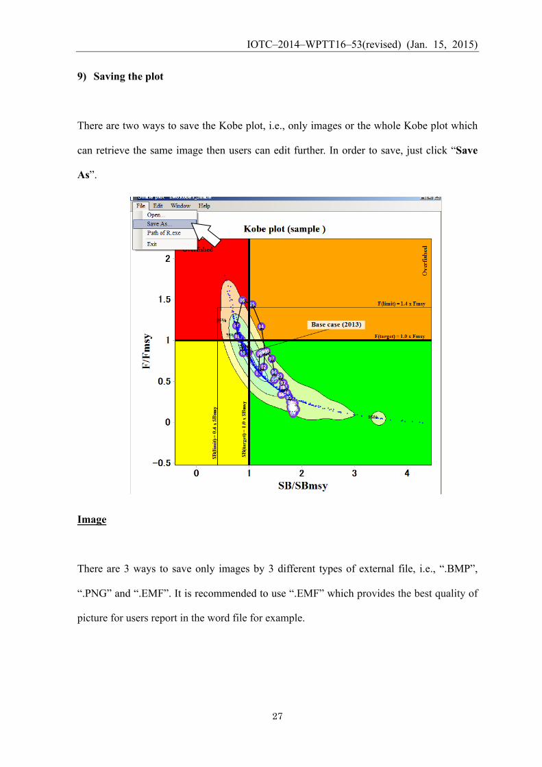
9) Saving the plot

There are two ways to save the Kobe plot, i.e., only images or the whole Kobe plot which

can retrieve the same image then users can edit further. In order to save, just click “Save

As”.

Image

There are 3 ways to save only images by 3 different types of external file, i.e., “.BMP”,

“.PNG” and “.EMF”. It is recommended to use “.EMF” which provides the best quality of

picture for users report in the word file for example.


28

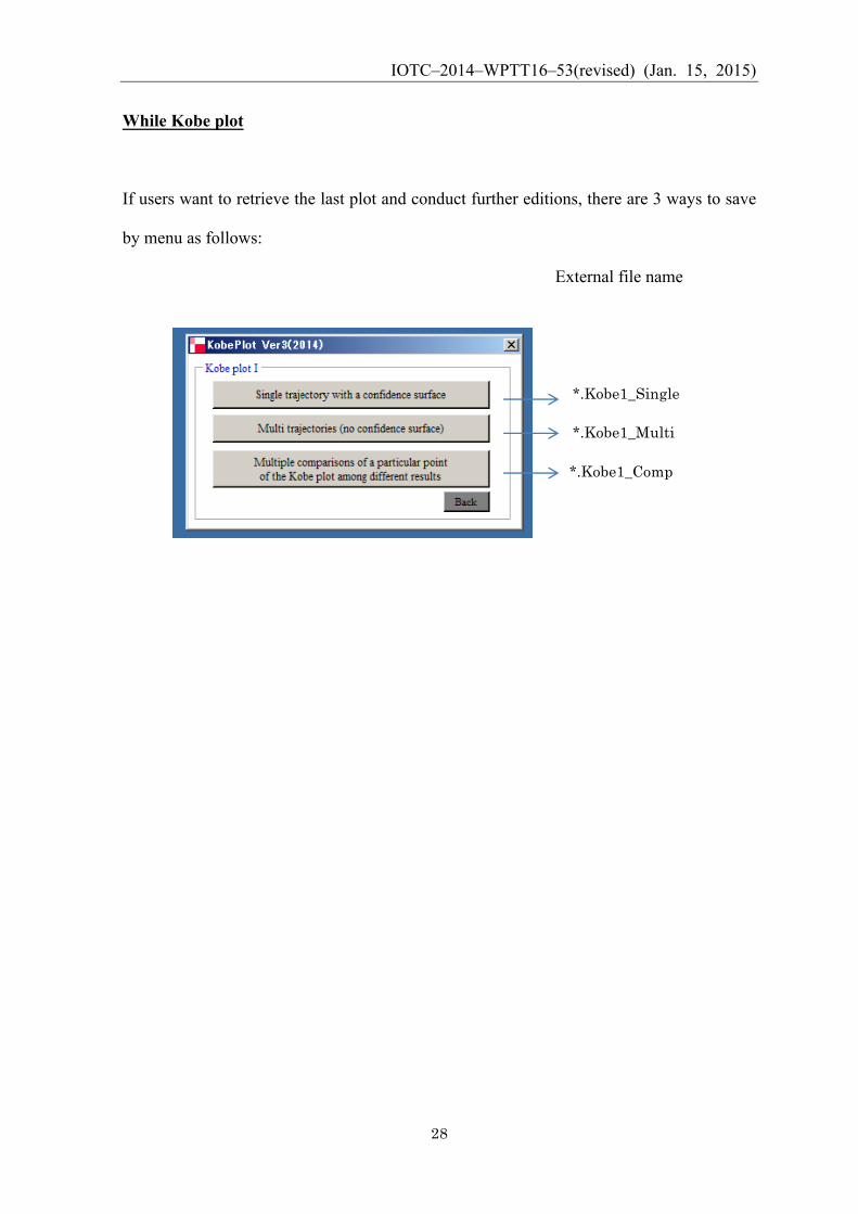
While Kobe plot

If users want to retrieve the last plot and conduct further editions, there are 3 ways to save

by menu as follows:

External file name

*.Kobe1_Single

*.Kobe1_Multi

*.Kobe1_Comp


29

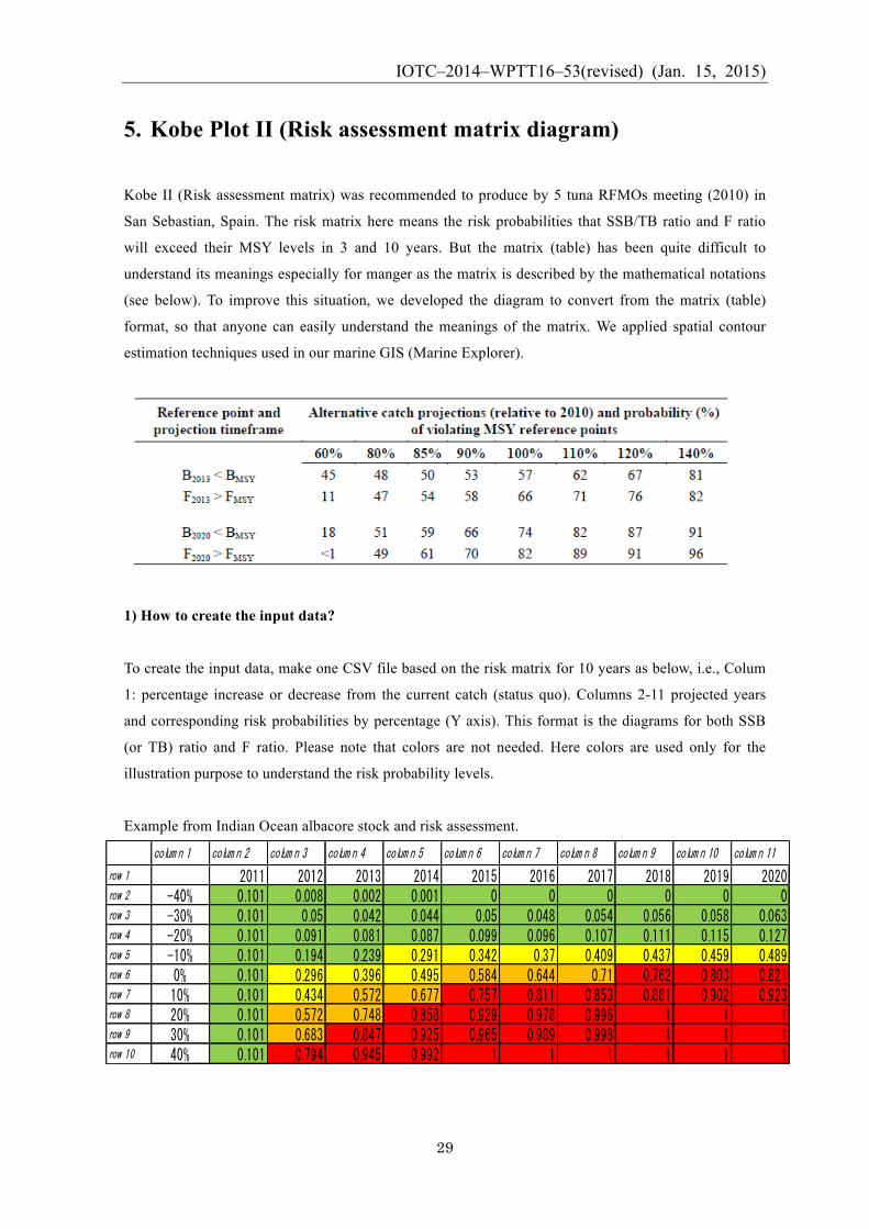
5. Kobe Plot II (Risk assessment matrix diagram)

Kobe II (Risk assessment matrix) was recommended to produce by 5 tuna RFMOs meeting (2010) in

San Sebastian, Spain. The risk matrix here means the risk probabilities that SSB/TB ratio and F ratio

will exceed their MSY levels in 3 and 10 years. But the matrix (table) has been quite difficult to

understand its meanings especially for manger as the matrix is described by the mathematical notations

(see below). To improve this situation, we developed the diagram to convert from the matrix (table)

format, so that anyone can easily understand the meanings of the matrix. We applied spatial contour

estimation techniques used in our marine GIS (Marine Explorer).


To create the input data, make one CSV file based on the risk matrix for 10 years as below, i.e., Colum

1: percentage increase or decrease from the current catch (status quo). Columns 2-11 projected years

and corresponding risk probabilities by percentage (Y axis). This format is the diagrams for both SSB

(or TB) ratio and F ratio. Please note that colors are not needed. Here colors are used only for the

illustration purpose to understand the risk probability levels.

Example from Indian Ocean albacore stock and risk assessment.

colum n 1 colum n 2 colum n 3 colum n 4 colum n 5 colum n 6 colum n 7 colum n 8 colum n 9 colum n 10 colum n 11

row 1 2011 2012 2013 2014 2015 2016 2017 2018 2019 2020row 2 -40% 0.101 0.008 0.002 0.001 0 0 0 0 0 0row 3 -30% 0.101 0.05 0.042 0.044 0.05 0.048 0.054 0.056 0.058 0.063row 4 -20% 0.101 0.091 0.081 0.087 0.099 0.096 0.107 0.111 0.115 0.127row 5 -10% 0.101 0.194 0.239 0.291 0.342 0.37 0.409 0.437 0.459 0.489row 6 0% 0.101 0.296 0.396 0.495 0.584 0.644 0.71 0.762 0.803 0.821row 7 10% 0.101 0.434 0.572 0.677 0.757 0.811 0.853 0.881 0.902 0.923row 8 20% 0.101 0.572 0.748 0.858 0.929 0.978 0.996 1 1 1row 9 30% 0.101 0.683 0.847 0.925 0.965 0.989 0.998 1 1 1row 10 40% 0.101 0.794 0.945 0.992 1 1 1 1 1 1


30

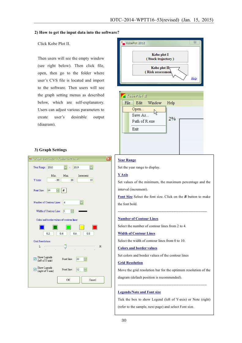
2) How to get the input data into the software?

3) Graph Settings

Year Range

Set the year range to display.

Y Axis

Set values of the minimum, the maximum percentage and the

interval (increment).

Font Size Select the font size. Click on the B button to make

the font bold.

-------------------------------------------------------------------------

Number of Contour Lines

Select the number of contour lines from 2 to 4.

Width of Contour Lines

Select the width of contour lines from 0 to 10.

Colors and border values

Set colors and border values of the contour lines

Grid Resolution

Move the grid resolution bar for the optimum resolution of the

diagram (default position is recommended).

-------------------------------------------------------------------------

Legends/Note and Font size

Tick the box to show Legend (left of Y-axis) or Note (right)

(refer to the sample, next page) and select Font size.

Click Kobe Plot II.

Then users will see the empty window

(see right below). Then click file,

open, then go to the folder where

user’s CVS file is located and import

to the software. Then users will see

the graph setting menus as described

below, which are self-explanatory.

Users can adjust various parameters to

create user’s desirable output

(diagram).


31

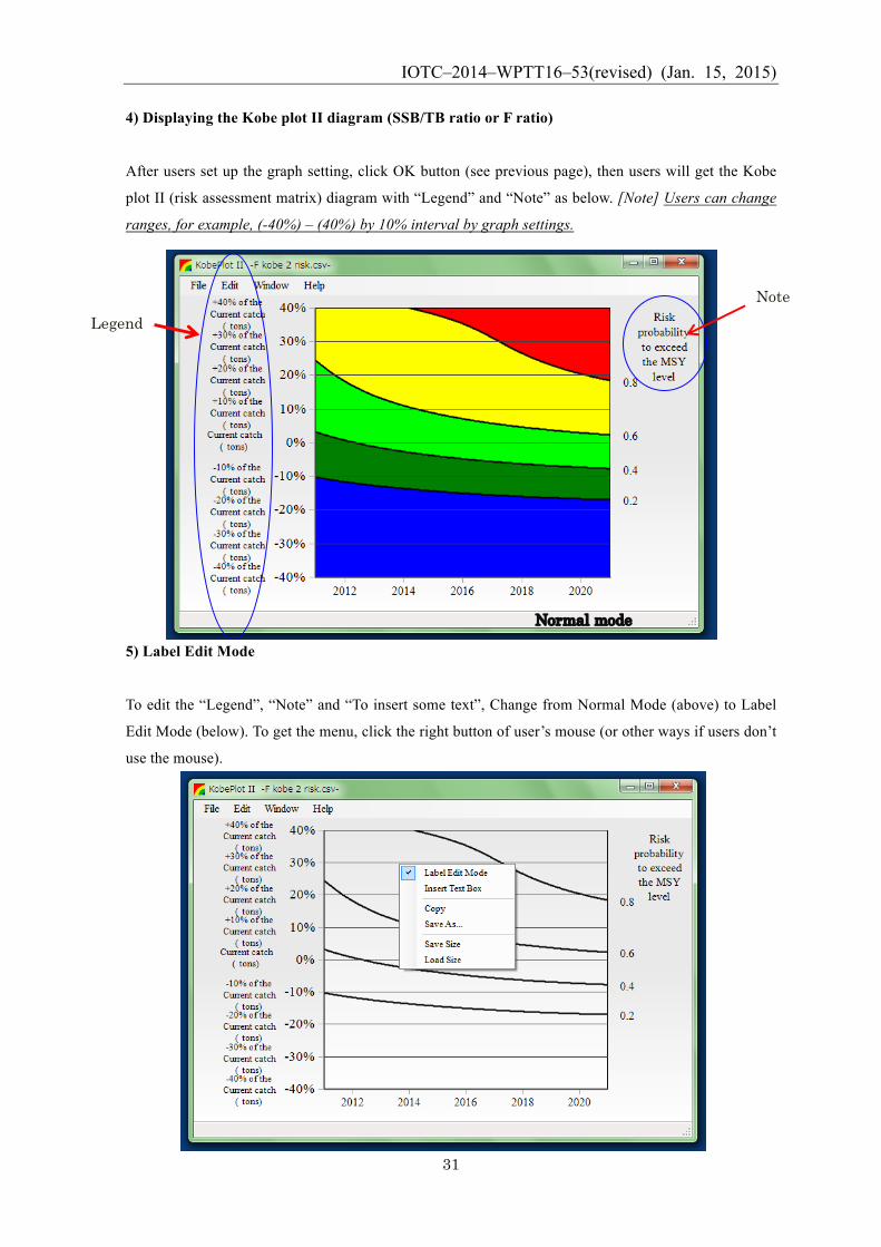
4) Displaying the Kobe plot II diagram (SSB/TB ratio or F ratio)

After users set up the graph setting, click OK button (see previous page), then users will get the Kobe

plot II (risk assessment matrix) diagram with “Legend” and “Note” as below. [Note] Users can change

ranges, for example, (-40%) – (40%) by 10% interval by graph settings.

5) Label Edit Mode

To edit the “Legend”, “Note” and “To insert some text”, Change from Normal Mode (above) to Label

Edit Mode (below). To get the menu, click the right button of user’s mouse (or other ways if users don’t

use the mouse).

Normal mode

Note Legend


32

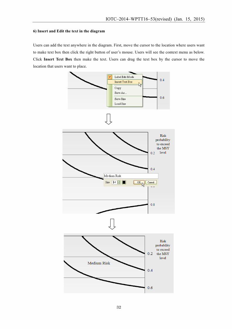
6) Insert and Edit the text in the diagram

Users can add the text anywhere in the diagram. First, move the cursor to the location where users want

to make text box then click the right button of user’s mouse. Users will see the context menu as below.

Click Insert Text Box then make the text. Users can drag the text box by the cursor to move the

location that users want to place.


33

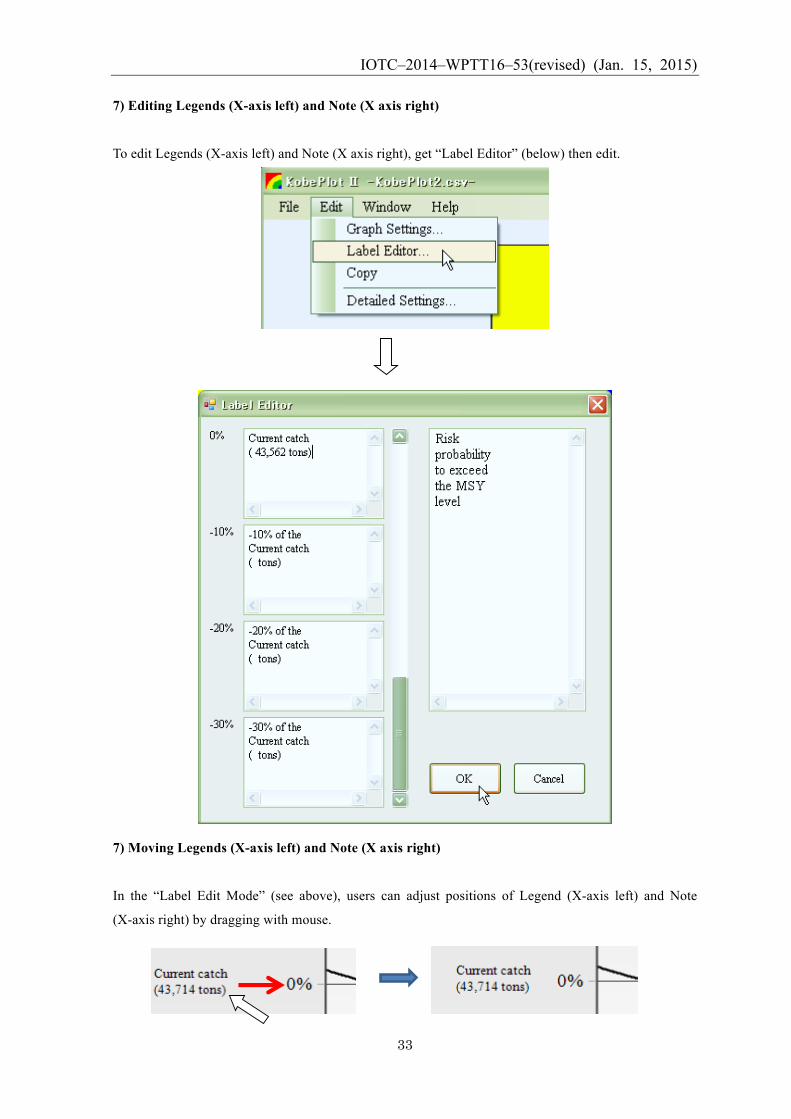
7) Editing Legends (X-axis left) and Note (X axis right)

To edit Legends (X-axis left) and Note (X axis right), get “Label Editor” (below) then edit.

7) Moving Legends (X-axis left) and Note (X axis right)

In the “Label Edit Mode” (see above), users can adjust positions of Legend (X-axis left) and Note

(X-axis right) by dragging with mouse.


34

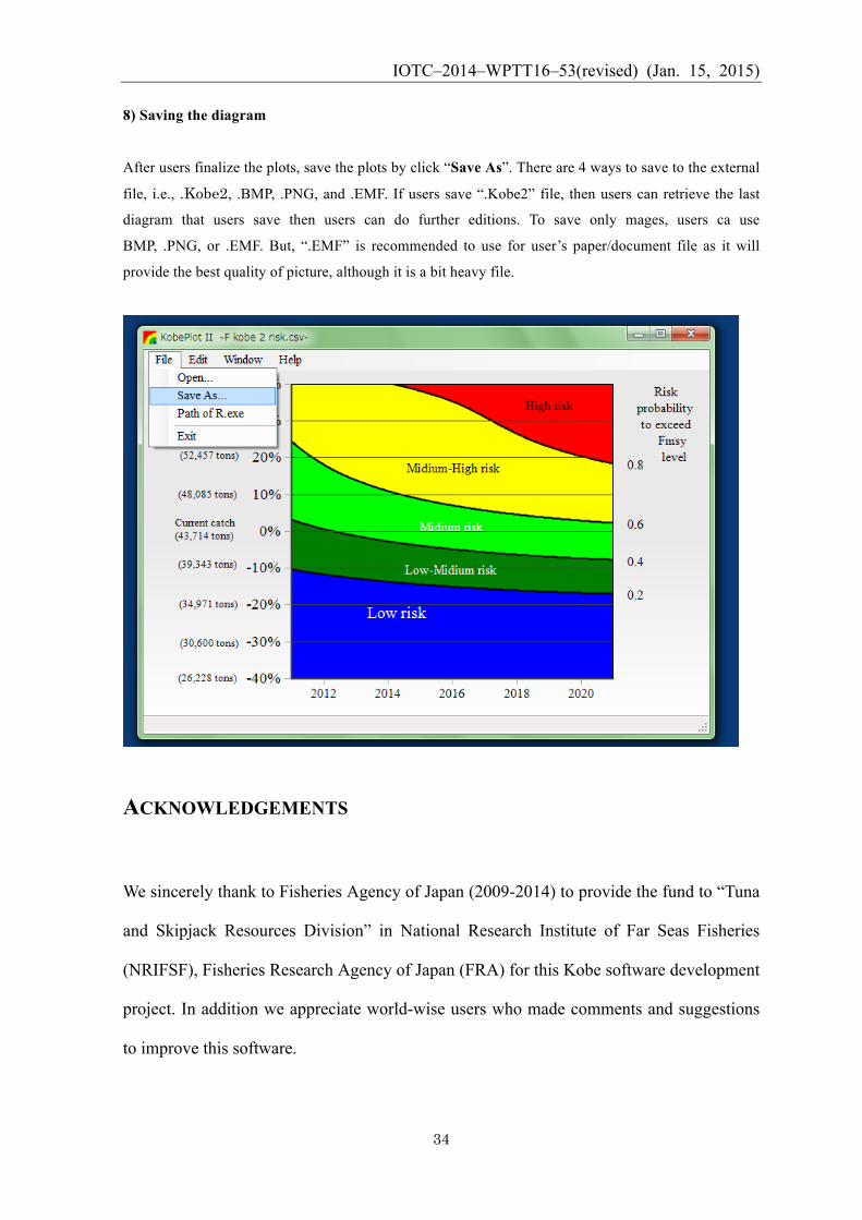
8) Saving the diagram

After users finalize the plots, save the plots by click “Save As”. There are 4 ways to save to the external

file, i.e., .Kobe2, .BMP, .PNG, and .EMF. If users save “.Kobe2” file, then users can retrieve the last

diagram that users save then users can do further editions. To save only mages, users ca use

BMP, .PNG, or .EMF. But, “.EMF” is recommended to use for user’s paper/document file as it will

provide the best quality of picture, although it is a bit heavy file.

ACKNOWLEDGEMENTS

We sincerely thank to Fisheries Agency of Japan (2009-2014) to provide the fund to “Tuna

and Skipjack Resources Division” in National Research Institute of Far Seas Fisheries

(NRIFSF), Fisheries Research Agency of Japan (FRA) for this Kobe software development

project. In addition we appreciate world-wise users who made comments and suggestions

to improve this software.


35

REFERENCES Kell, L.T. (2011): A STANDARDISED WAY OF PRESENTING SPECIES GROUP

EXECUTIVE SUMARISES. ICCAT/SCRS/2010/138, Collect. Vol. Sci. Pap. ICCAT 66(5): 2213-2228.

Kell, L.T.: Kobe - R tools for Tuna Management Advice (ICCAT). Maunder, M.N. and Aires-da-Silva, A. (2011): EVALUATION OF THE KOBE PLOT AND

STRATEGY MATRIX AND THEIR APPLICATION TO TUNA IN THE EPO. Restrepo, V. (2011): Stock Assessment 101 - Current Practice for Tuna Stocks, Chair, ISSF

Scientific Advisory Committee.

APPENDIX A: SPECIFICATION OF KOBE I AND II SOFTWARE

General

l Operation Systems (OS) : MS windows OS (both 32 and 64-bit PCs)

l Microsoft Visual Studio 2010 (general programming)

l TeeChart Pro .NET v2010 (graphical components)

Copyright © 2010 by Steema Software SL

Confidence surface in Kobe plot I and contour estimations in Kobe plot (diagram) II

Following functions in “R” are applied

Confidence surface

l ‘kde2d’ function : Kernel estimation

Kobe plots 2 (Contour estimation of the diagram)

l ‘surf.gls’ function :to assign contour surface by least square means

l ‘prmat’ function: to assign the contour line by kriging

Documents

Kobe I (Kobe plot) +Kobe II (risk assessment) software Material/Stock... · IOTC–2014–WPTT16–53(revised) (Jan. 15, 2015) 4 2 Installation 1) Uninstall the old versions of Kobe