KRIGING WITH ESTIMATEDPARAMETERS

Richard L. Smith

Department of Statistics and Operations Research

University of North Carolina

Chapel Hill

Iowa State University

September 12 2005

Acknowledgements to:

Zhengyuan Zhu

Elizabeth Shamseldin

Stas Kolenikov

Joe Ibrahim

1

References

For a preliminary version of a paper on this talk is based, see:

Smith, R.L. and Zhu, Z. (2004), Asymptotic theory for kriging

with estimated parameters and its application to network design.

http://www.stat.unc.edu/postscript/rs/supp5.pdf

For background about the PM2.5 application:

R.L. Smith, S. Kolenikov and L.H. Cox (2003), Spatio-temporal

modeling of PM2.5 data with missing values. J. Geophys. Res.,

108(D24), 9004, doi:10.1029/2002JD002914, 2003.

http://www.stat.unc.edu/postscript/rs/Smith-JGR-2003.pdf

2

I Motivating Example: Interpolation of Air Pollution Data

II Universal Kriging, REML Estimation and Bayesian Spatial Statis-

tics

III Existing Results on “Kriging With Estimated Parameters”

IV The Approach Based on Second-Order Asymptotics

V Example Based on PM2.5 Monitors in North Carolina

3

I. Motivating Example: Interpolation of Air Pollution Data

The problems of spatial interpolation and network design are

introduced through an example using the EPA fine particulates

(PM2.5) network. The analysis is taken from Smith, Kolenikov

and Cox (2003).

4

Current EPA standard for PM2.5:

• Twenty-four hour average PM2.5 not to exceed 65 µg/m3

for a three-year average of annual 98th percentiles at any

population-oriented monitoring site in a monitoring area.

• Three-year annual average PM2.5 not to exceed 15 µg/m3

concentrations from a single community-oriented monitor-

ing site or the spatial average of eligible community-oriented

monitoring sites in a monitoring area.

5

The data (compiled from a larger data set) consisted of weekly

average PM2.5 levels during 1999 at 74 EPA stations in NC, SC,

GA. We fitted a model of the form

yxt = f(x) + g(t) + ηxt

in which yxt is the square root of PM2.5 in location x in week t,

f(x) and g(t) are fixed functions of time and space respectively

(both represented as linear regression functions), and ηxt is a

random error (independent in time but dependent in space).

The model parameters were estimated by maximum likelihood,

and kriging (described later) was used to interpolate ηxt at loca-

tions x off the network. Based on that, a map was constructed

of the interpolated annual average for each point in the study

region, together with an estimated root mean square prediction

error.

6

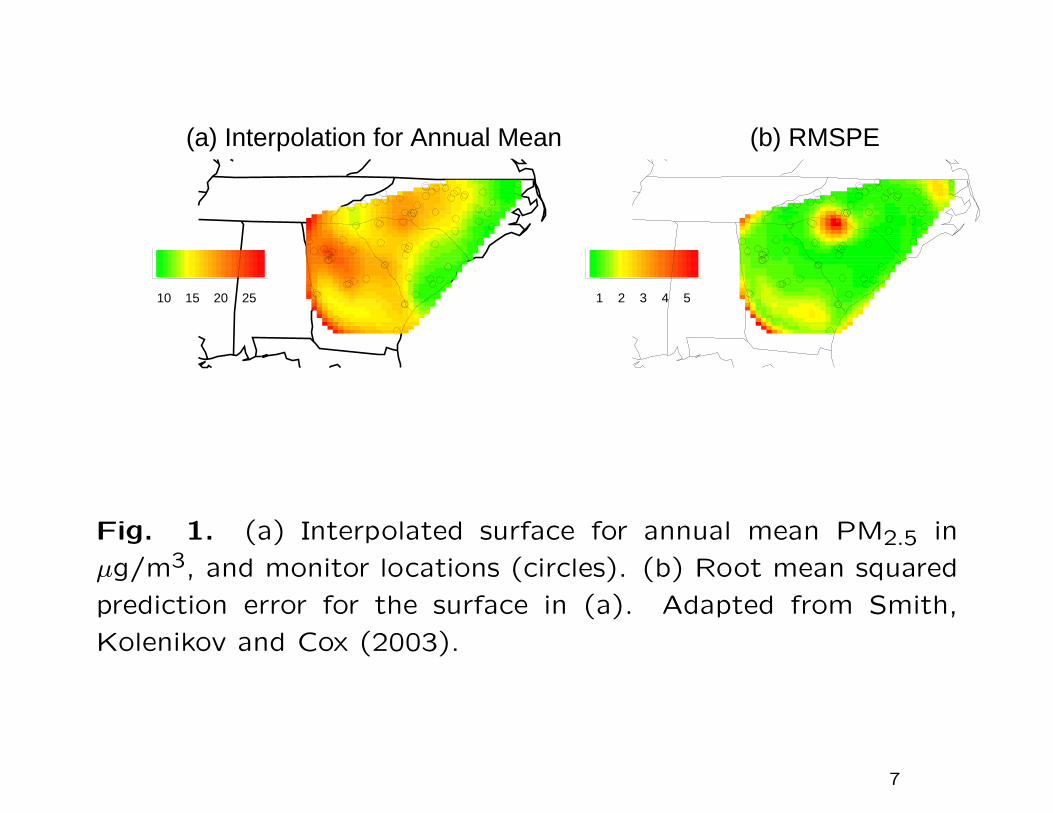
10 15 20 25

(a) Interpolation for Annual Mean

1 2 3 4 5

(b) RMSPE

Fig. 1. (a) Interpolated surface for annual mean PM2.5 in

µg/m3, and monitor locations (circles). (b) Root mean squared

prediction error for the surface in (a). Adapted from Smith,

Kolenikov and Cox (2003).

7

10 15 20 25

(a) Interpolation for Annual Mean

1 2 3 4 5

(b) RMSPE

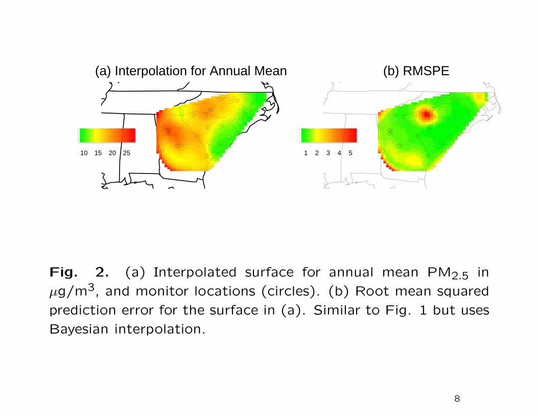
Fig. 2. (a) Interpolated surface for annual mean PM2.5 in

µg/m3, and monitor locations (circles). (b) Root mean squared

prediction error for the surface in (a). Similar to Fig. 1 but uses

Bayesian interpolation.

8

Questions for this talk:

There are many questions along the lines of what is the rightmodel for this data set, but in this talk, I focus on two moretheoretical aspects:

1. Computation of RMSPEs. The calculations above used theconventional formulae for kriging prediction errors that youcan find in any text on geostatistics, but these ignore modelestimation errors. Is this appropriate, and how could weimprove on this approach?

2. Design of the network. The EPA is constantly adding ordeleting stations as it attempts to provide better coverageor to reduce costs. How could it do this most efficiently?

The two questions are linked because accurate determination ofkriging errors is critical in assessing the design.

9

II. Universal Kriging, REML Estimation and Bayesian

Spatial Statistics

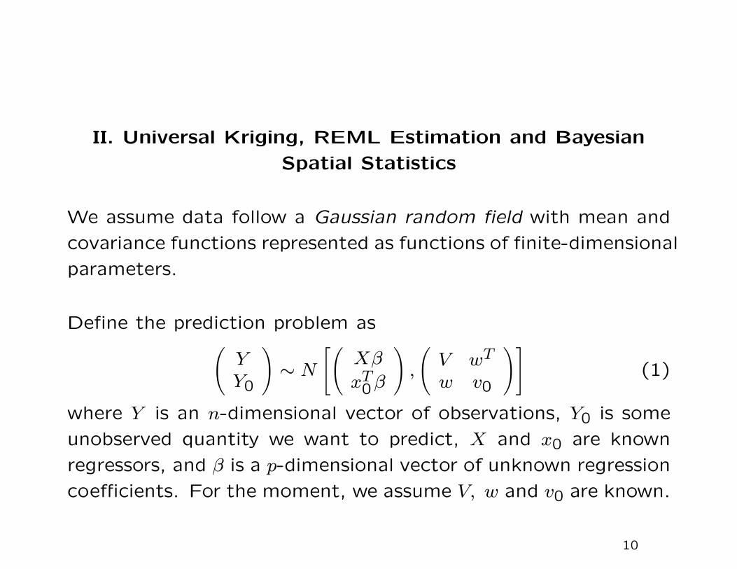
We assume data follow a Gaussian random field with mean and

covariance functions represented as functions of finite-dimensional

parameters.

Define the prediction problem as(YY0

)∼ N

[(Xβ

xT0β

),

(V wT

w v0

)](1)

where Y is an n-dimensional vector of observations, Y0 is some

unobserved quantity we want to predict, X and x0 are known

regressors, and β is a p-dimensional vector of unknown regression

coefficients. For the moment, we assume V, w and v0 are known.

10

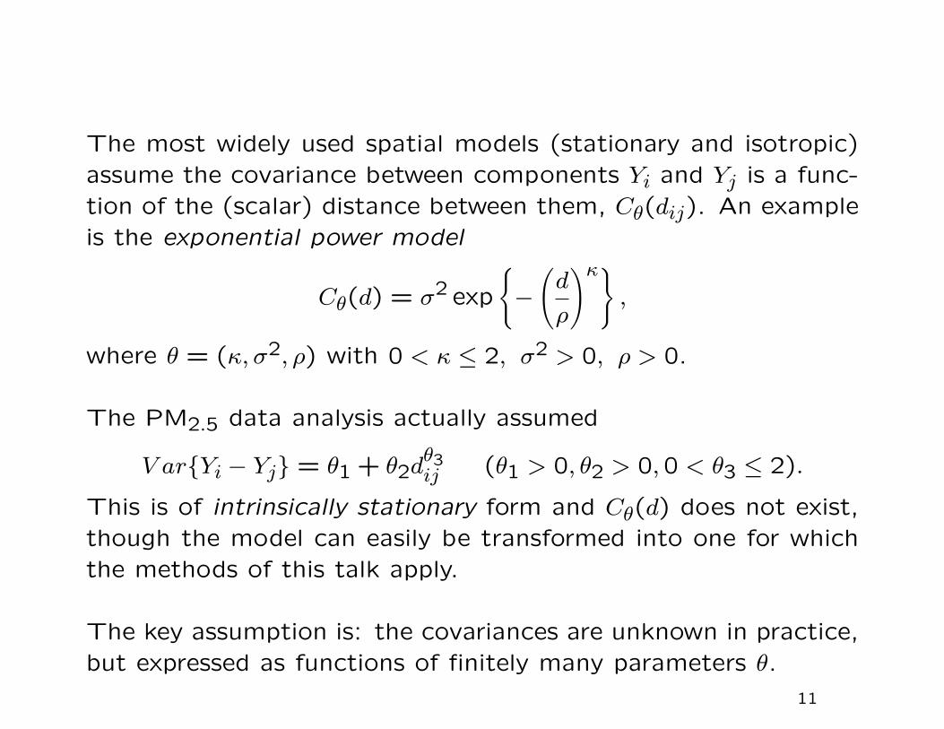
The most widely used spatial models (stationary and isotropic)assume the covariance between components Yi and Yj is a func-tion of the (scalar) distance between them, Cθ(dij). An exampleis the exponential power model

Cθ(d) = σ2 exp

{−(d

ρ

)κ},

where θ = (κ, σ2, ρ) with 0 < κ ≤ 2, σ2 > 0, ρ > 0.

The PM2.5 data analysis actually assumed

V ar{Yi − Yj} = θ1 + θ2dθ3ij (θ1 > 0, θ2 > 0,0 < θ3 ≤ 2).

This is of intrinsically stationary form and Cθ(d) does not exist,though the model can easily be transformed into one for whichthe methods of this talk apply.

The key assumption is: the covariances are unknown in practice,but expressed as functions of finitely many parameters θ.

11

Universal Kriging

Assume model (1) where the covariances V, w, v0 are known but

β is unknown. The classical formulation of universal kriging asks

for a predictor Y0 = λTY that minimizes σ20 = E

{(Y0 − Y0)

2}

subject to the unbiasedness condition E{Y0 − Y0

}= 0.

The classical solution:

λ = wTV −1 + (x0 −XTV −1w)T (XTV −1X)−1XTV −1,

σ20 = v0 − wTV −1w+ (x0 −XTV −1w)T (XTV −1X)−1(x0 −XTV −1w).

12

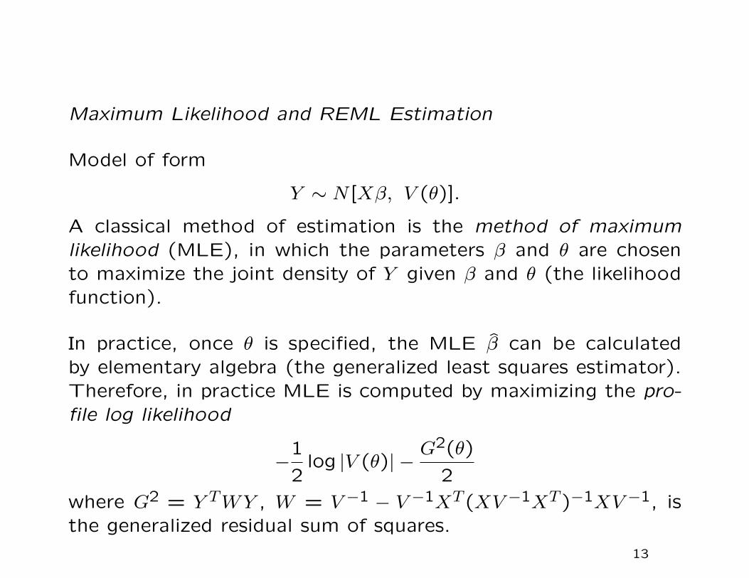
Maximum Likelihood and REML Estimation

Model of form

Y ∼ N [Xβ, V (θ)].

A classical method of estimation is the method of maximumlikelihood (MLE), in which the parameters β and θ are chosento maximize the joint density of Y given β and θ (the likelihoodfunction).

In practice, once θ is specified, the MLE β can be calculatedby elementary algebra (the generalized least squares estimator).Therefore, in practice MLE is computed by maximizing the pro-file log likelihood

−1

2log |V (θ)| −

G2(θ)

2

where G2 = Y TWY , W = V −1 − V −1XT (XV −1XT )−1XV −1, isthe generalized residual sum of squares.

13

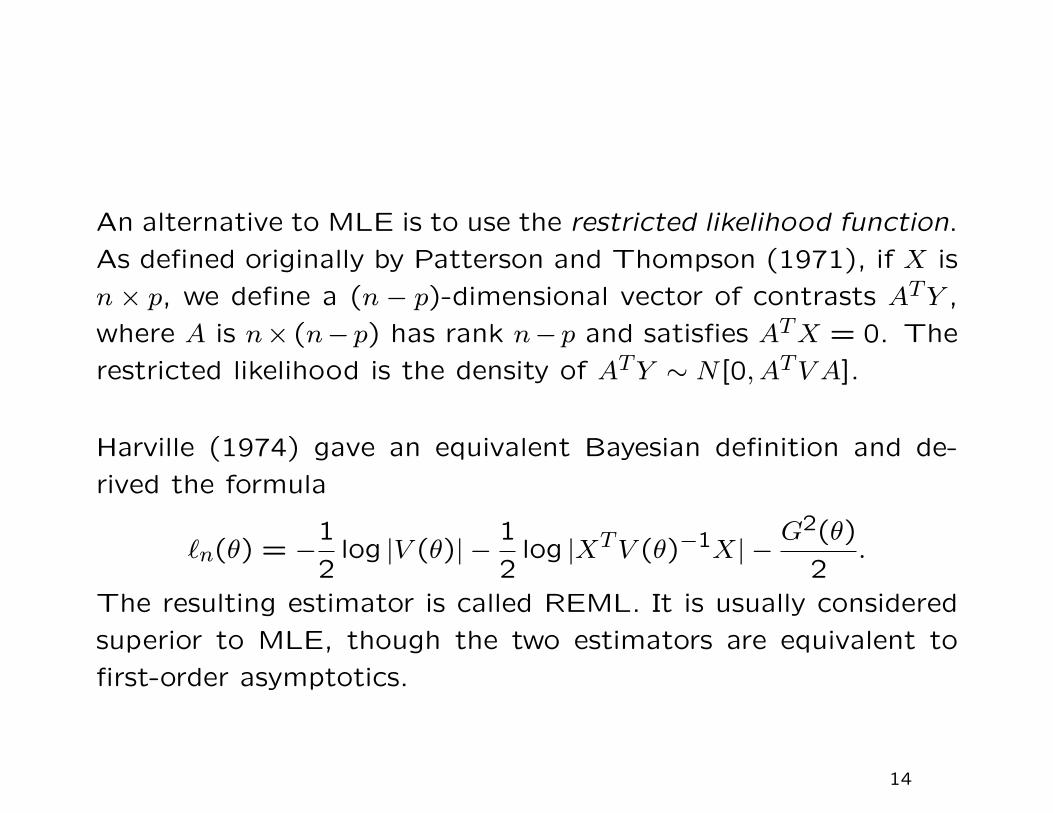
An alternative to MLE is to use the restricted likelihood function.

As defined originally by Patterson and Thompson (1971), if X is

n × p, we define a (n − p)-dimensional vector of contrasts ATY ,

where A is n× (n− p) has rank n− p and satisfies ATX = 0. The

restricted likelihood is the density of ATY ∼ N [0, ATV A].

Harville (1974) gave an equivalent Bayesian definition and de-

rived the formula

`n(θ) = −1

2log |V (θ)| −

1

2log |XTV (θ)−1X| −

G2(θ)

2.

The resulting estimator is called REML. It is usually considered

superior to MLE, though the two estimators are equivalent to

first-order asymptotics.

14

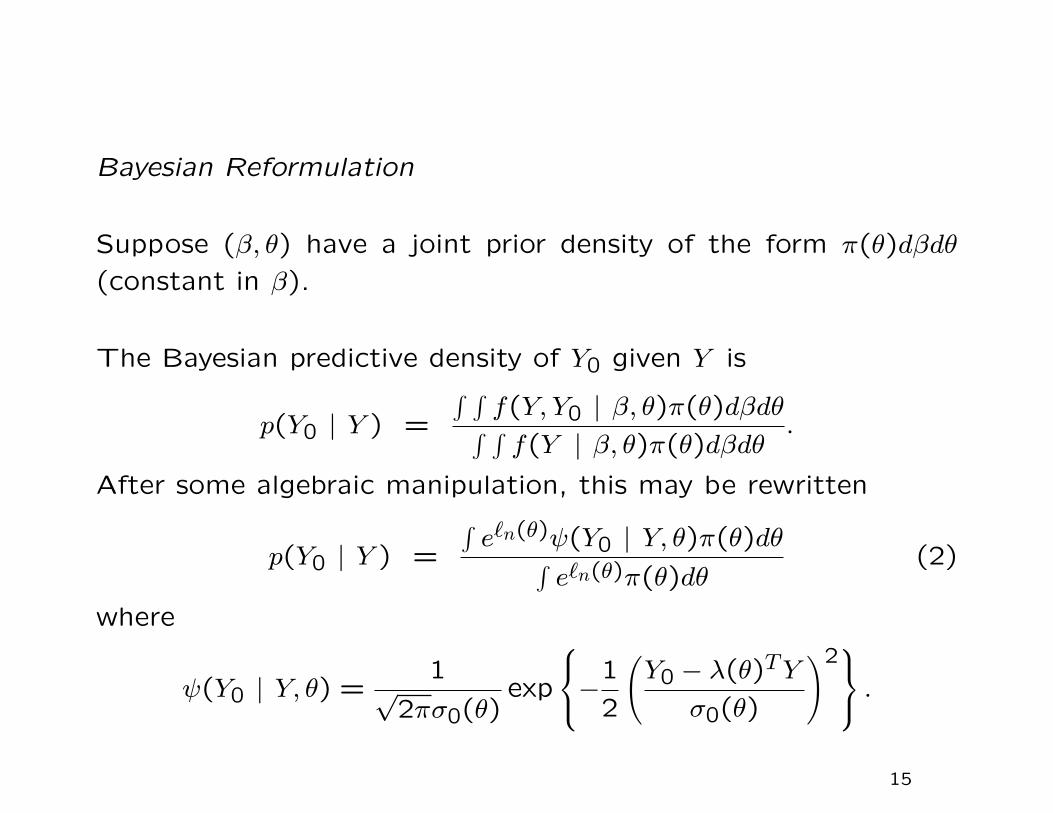
Bayesian Reformulation

Suppose (β, θ) have a joint prior density of the form π(θ)dβdθ

(constant in β).

The Bayesian predictive density of Y0 given Y is

p(Y0 | Y ) =

∫ ∫f(Y, Y0 | β, θ)π(θ)dβdθ∫ ∫f(Y | β, θ)π(θ)dβdθ

.

After some algebraic manipulation, this may be rewritten

p(Y0 | Y ) =

∫e`n(θ)ψ(Y0 | Y, θ)π(θ)dθ∫

e`n(θ)π(θ)dθ(2)

where

ψ(Y0 | Y, θ) =1√

2πσ0(θ)exp

−1

2

(Y0 − λ(θ)TY

σ0(θ)

)2 .

15

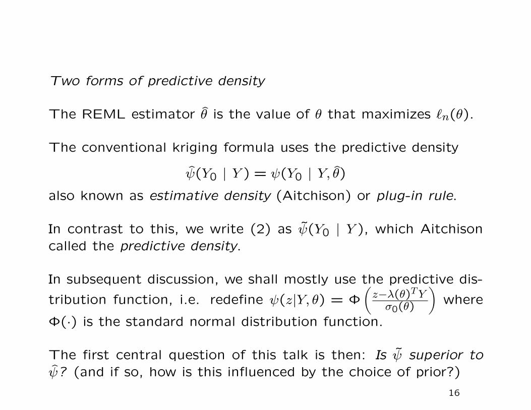
Two forms of predictive density

The REML estimator θ is the value of θ that maximizes `n(θ).

The conventional kriging formula uses the predictive density

ψ(Y0 | Y ) = ψ(Y0 | Y, θ)also known as estimative density (Aitchison) or plug-in rule.

In contrast to this, we write (2) as ψ(Y0 | Y ), which Aitchisoncalled the predictive density.

In subsequent discussion, we shall mostly use the predictive dis-

tribution function, i.e. redefine ψ(z|Y, θ) = Φ(z−λ(θ)TYσ0(θ)

)where

Φ(·) is the standard normal distribution function.

The first central question of this talk is then: Is ψ superior toψ? (and if so, how is this influenced by the choice of prior?)

16

Designing Monitor Networks

Large literature, many different approaches.

Recent work has focussed on contrast between two types ofcriterion:

• Estimative — e.g. choose the design to maximize the deter-minant of the Fisher information matrix of θ

• Predictive — focus on a specific Y0, find a design to minimizeσ0. Note that this ignores the estimation of θ, in effectassuming θ known.

Zhu and Stein (2004) discussed the idea of using Bayesian predic-tion intervals as a basis for network design, arguing that Bayesianintervals take account of the uncertainty of θ and thereforeshould be superior to the predictive approach. However, theyrejected this as too computationally intensive, and instead pro-posed a two-stage criterion (more later).

17

Direct Bayesian Approach

• For any data set, use MCMC to construct the Bayesian pre-

dictive distribution

• For any given design, run the Bayesian analysis on simulated

data sets to determine the expected length of Bayesian pre-

diction intervals

• Use an optimization algorithm (e.g. simulated annealing) to

find the optimal design

Direct implementation of this approach requires a lot of Monte

Carlo simulation. The second major theme of this talk is to pro-

pose an approximate approach that reduces the first two steps to

a simple algebraic formula for the expected length of a Bayesian

prediction interval.

18

III Existing Results on “Kriging With EstimatedParameters”

Suppose we apply universal kriging to predict Y0 by λTY , butestimate λ = λ(θ) where θ is the MLE or REMLE.

Harville and Jeske (1992) and Zimmerman and Cressie (1992)proposed the following correction to the mean squared predictionerror:

V1 = E{(Y0 − λTY )2

}≈ σ2

0 + tr

{I−1

(∂λ

∂θ

)TV

(∂λ

∂θ

)}where I is the observed information matrix for θ. This formulacorrects for the error in specifying the kriging weights λ.

The derivation of this formula assumed that θ−θ was independentof Y0 − λTY . Abt (1999) derived an improved formula withoutthis assumption, but noted that in practice, the improvementmade little difference to the result.

19

However, in calculating a prediction interval for Y0, it is also

necessary to consider the effect of σ20 being unknown. Stein

(1999) and Zhu and Stein (2004) defined

V2 =

(∂σ2

0

∂θ

)TI−1

(∂σ2

0

∂θ

)

as a measure of the uncertainty in σ20, and they suggested that

some linear combination of V1 and V2σ20

would best measure the

overall uncertainty. In particular, they suggested

V3 = V1 +1

2·V2

σ20

as a suitable combined criterion. However, it’s not clear exactly

why this particular linear combination is appropriate.

20

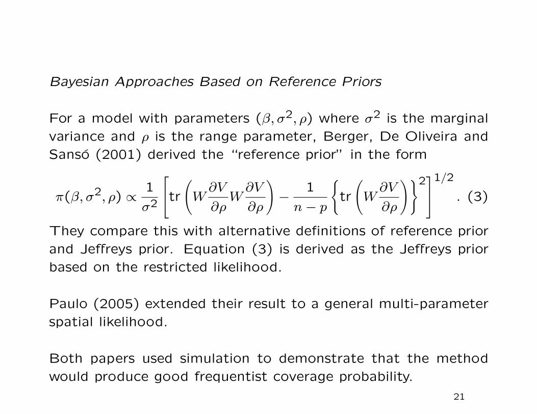
Bayesian Approaches Based on Reference Priors

For a model with parameters (β, σ2, ρ) where σ2 is the marginal

variance and ρ is the range parameter, Berger, De Oliveira and

Sanso (2001) derived the “reference prior” in the form

π(β, σ2, ρ) ∝1

σ2

tr(W∂V

∂ρW∂V

∂ρ

)−

1

n− p

{tr

(W∂V

∂ρ

)}21/2 . (3)

They compare this with alternative definitions of reference prior

and Jeffreys prior. Equation (3) is derived as the Jeffreys prior

based on the restricted likelihood.

Paulo (2005) extended their result to a general multi-parameter

spatial likelihood.

Both papers used simulation to demonstrate that the method

would produce good frequentist coverage probability.

21

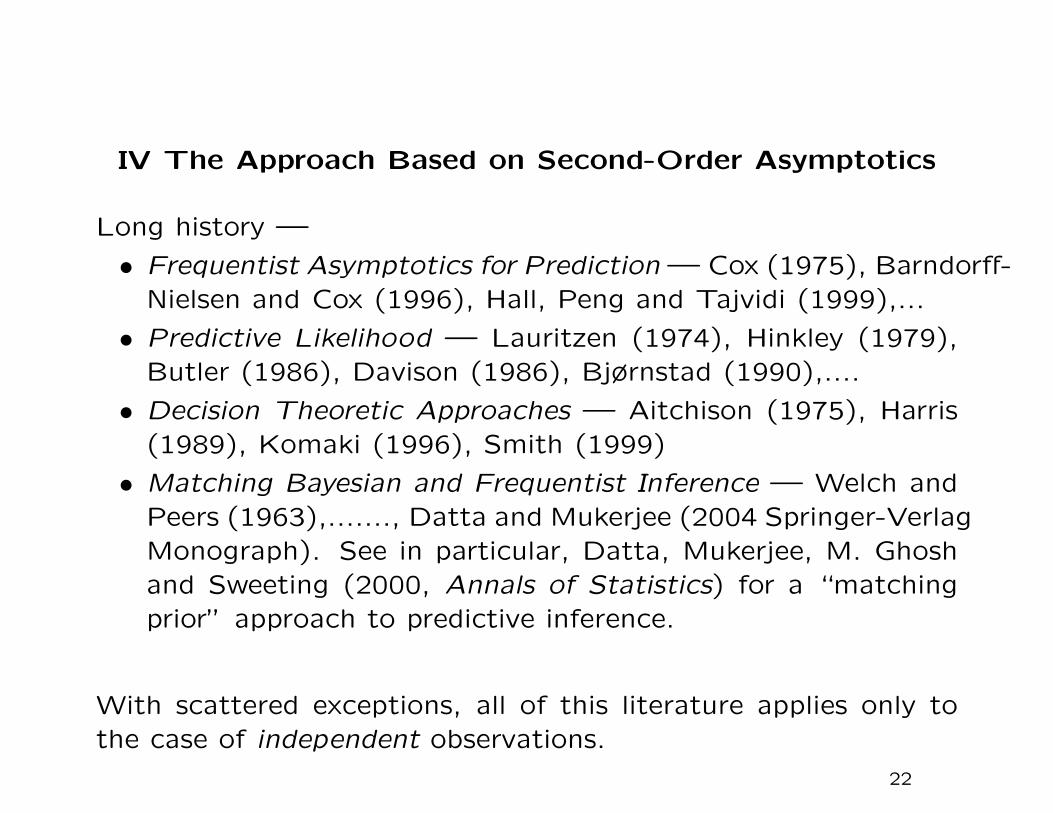
IV The Approach Based on Second-Order Asymptotics

Long history —

• Frequentist Asymptotics for Prediction — Cox (1975), Barndorff-Nielsen and Cox (1996), Hall, Peng and Tajvidi (1999),...

• Predictive Likelihood — Lauritzen (1974), Hinkley (1979),Butler (1986), Davison (1986), Bjørnstad (1990),....

• Decision Theoretic Approaches — Aitchison (1975), Harris(1989), Komaki (1996), Smith (1999)

• Matching Bayesian and Frequentist Inference — Welch andPeers (1963),......., Datta and Mukerjee (2004 Springer-VerlagMonograph). See in particular, Datta, Mukerjee, M. Ghoshand Sweeting (2000, Annals of Statistics) for a “matchingprior” approach to predictive inference.

With scattered exceptions, all of this literature applies only tothe case of independent observations.

22

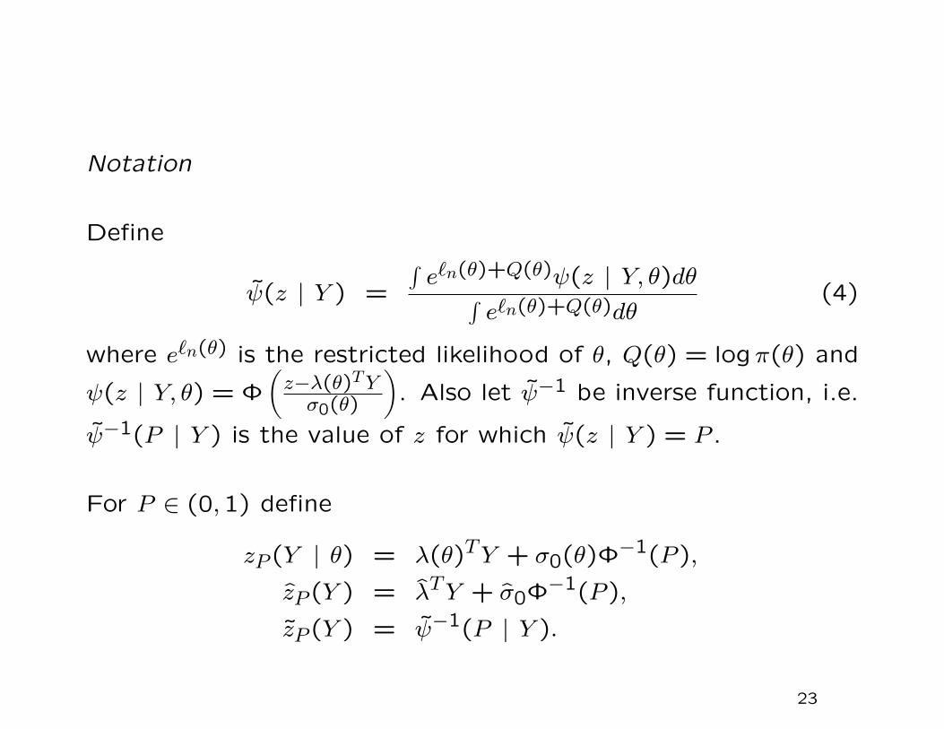
Notation

Define

ψ(z | Y ) =

∫e`n(θ)+Q(θ)ψ(z | Y, θ)dθ∫

e`n(θ)+Q(θ)dθ(4)

where e`n(θ) is the restricted likelihood of θ, Q(θ) = logπ(θ) and

ψ(z | Y, θ) = Φ(z−λ(θ)TYσ0(θ)

). Also let ψ−1 be inverse function, i.e.

ψ−1(P | Y ) is the value of z for which ψ(z | Y ) = P .

For P ∈ (0,1) define

zP (Y | θ) = λ(θ)TY + σ0(θ)Φ−1(P ),

zP (Y ) = λTY + σ0Φ−1(P ),

zP (Y ) = ψ−1(P | Y ).

23

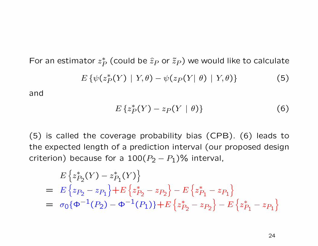
For an estimator z∗P (could be zP or zP ) we would like to calculate

E {ψ(z∗P (Y ) | Y, θ)− ψ(zP (Y | θ) | Y, θ)} (5)

and

E {z∗P (Y )− zP (Y | θ)} (6)

(5) is called the coverage probability bias (CPB). (6) leads to

the expected length of a prediction interval (our proposed design

criterion) because for a 100(P2 − P1)% interval,

E{z∗P2

(Y )− z∗P1(Y )

}= E

{zP2

− zP1

}+E

{z∗P2

− zP2

}− E

{z∗P1

− zP1

}= σ0{Φ−1(P2)−Φ−1(P1)}+E

{z∗P2

− zP2

}− E

{z∗P1

− zP1

}

24

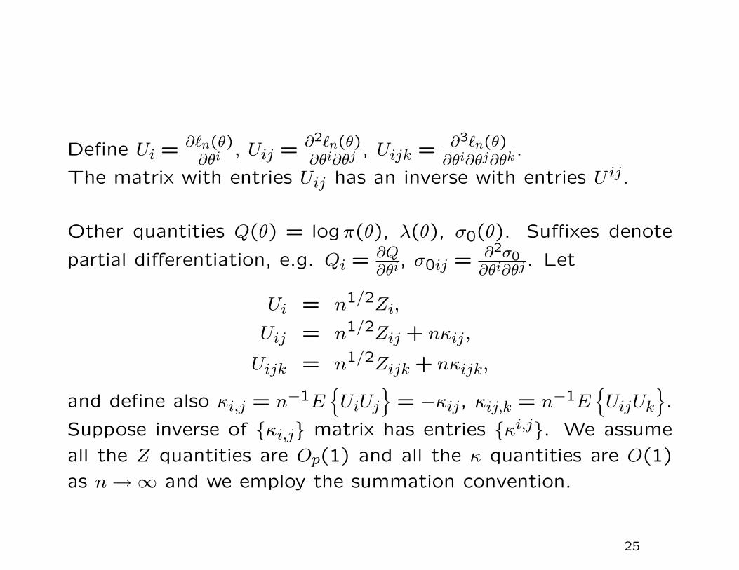
Define Ui =∂`n(θ)∂θi

, Uij = ∂2`n(θ)∂θi∂θj

, Uijk = ∂3`n(θ)∂θi∂θj∂θk

.

The matrix with entries Uij has an inverse with entries U ij.

Other quantities Q(θ) = logπ(θ), λ(θ), σ0(θ). Suffixes denote

partial differentiation, e.g. Qi =∂Q∂θi

, σ0ij = ∂2σ0∂θi∂θj

. Let

Ui = n1/2Zi,

Uij = n1/2Zij + nκij,

Uijk = n1/2Zijk + nκijk,

and define also κi,j = n−1E{UiUj

}= −κij, κij,k = n−1E

{UijUk

}.

Suppose inverse of {κi,j} matrix has entries {κi,j}. We assume

all the Z quantities are Op(1) and all the κ quantities are O(1)

as n→∞ and we employ the summation convention.

25

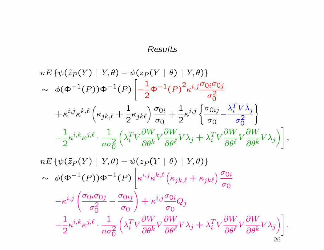
Results

nE {ψ(zP (Y ) | Y, θ)− ψ(zP (Y | θ) | Y, θ)}

∼ φ(Φ−1(P ))Φ−1(P )

[−

1

2Φ−1(P )

2κi,j

σ0iσ0j

σ20

+κi,jκk,`(κjk,` +

1

2κjk`

)σ0i

σ0+

1

2κi,j

{σ0ij

σ0−λTi V λj

σ20

}

−1

2κi,kκj,` ·

1

nσ20

(λTi V

∂W

∂θkV∂W

∂θ`V λj + λTi V

∂W

∂θ`V∂W

∂θkV λj

)],

nE {ψ(zP (Y ) | Y, θ)− ψ(zP (Y | θ) | Y, θ)}

∼ φ(Φ−1(P ))Φ−1(P )

[κi,jκk,`

(κjk,` + κjk`

) σ0i

σ0

−κi,j(σ0iσ0j

σ20

−σ0ij

σ0

)+ κi,j

σ0i

σ0Qj

−1

2κi,kκj,` ·

1

nσ20

(λTi V

∂W

∂θkV∂W

∂θ`V λj + λTi V

∂W

∂θ`V∂W

∂θkV λj

)].

26

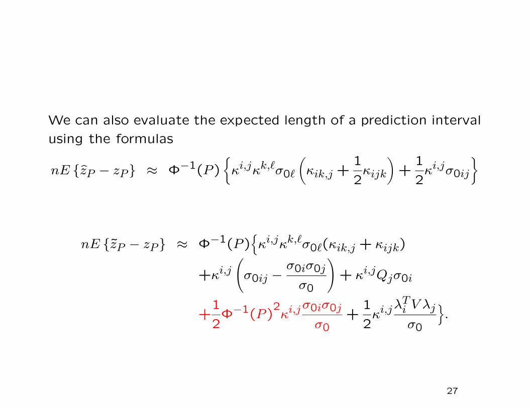
We can also evaluate the expected length of a prediction interval

using the formulas

nE {zP − zP} ≈ Φ−1(P ){κi,jκk,`σ0`

(κik,j +

1

2κijk

)+

1

2κi,jσ0ij

}

nE {zP − zP} ≈ Φ−1(P ){κi,jκk,`σ0`(κik,j + κijk)

+κi,j(σ0ij −

σ0iσ0j

σ0

)+ κi,jQjσ0i

+1

2Φ−1(P )

2κi,j

σ0iσ0j

σ0+

1

2κi,j

λTi V λj

σ0

}.

27

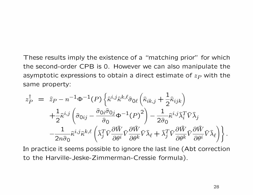
These results imply the existence of a “matching prior” for which

the second-order CPB is 0. However we can also manipulate the

asymptotic expressions to obtain a direct estimate of zP with the

same property:

z†P = zP − n−1Φ−1(P )

{κi,jκk,`σ0`

(κik,j +

1

2κijk

)+

1

2κi,j

(σ0ij −

σ0iσ0j

σ0Φ−1(P )

2)−

1

2σ0κi,jλTi V λj

−1

2nσ0κi,jκk,`

(λTj V

∂W

∂θiV∂W

∂θkV λ` + λTj V

∂W

∂θkV∂W

∂θiV λ`

)}.

In practice it seems possible to ignore the last line (Abt correction

to the Harville-Jeske-Zimmerman-Cressie formula).

28

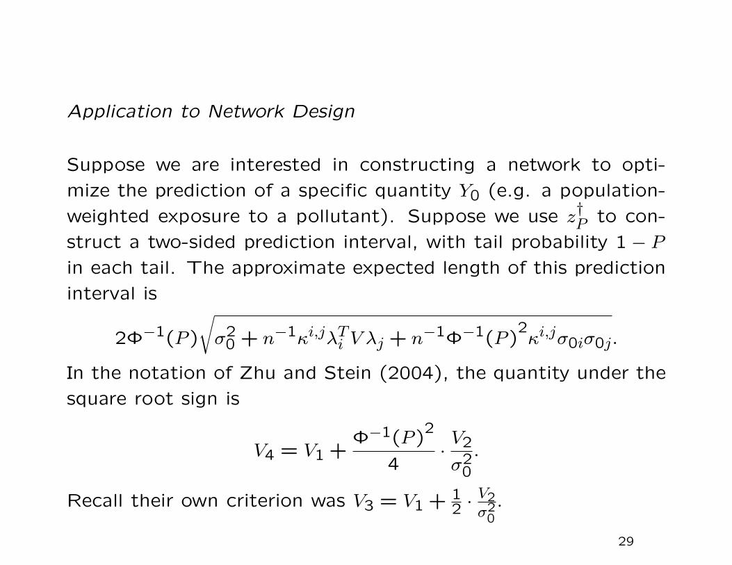
Application to Network Design

Suppose we are interested in constructing a network to opti-

mize the prediction of a specific quantity Y0 (e.g. a population-

weighted exposure to a pollutant). Suppose we use z†P to con-

struct a two-sided prediction interval, with tail probability 1− P

in each tail. The approximate expected length of this prediction

interval is

2Φ−1(P )

√σ20 + n−1κi,jλTi V λj + n−1Φ−1(P )

2κi,jσ0iσ0j.

In the notation of Zhu and Stein (2004), the quantity under the

square root sign is

V4 = V1 +Φ−1(P )

2

4·V2

σ20

.

Recall their own criterion was V3 = V1 + 12 ·

V2σ20.

29

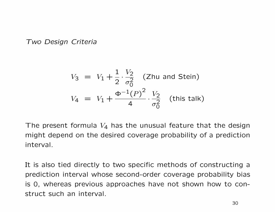
Two Design Criteria

V3 = V1 +1

2·V2

σ20

(Zhu and Stein)

V4 = V1 +Φ−1(P )

2

4·V2

σ20

(this talk)

The present formula V4 has the unusual feature that the design

might depend on the desired coverage probability of a prediction

interval.

It is also tied directly to two specific methods of constructing a

prediction interval whose second-order coverage probability bias

is 0, whereas previous approaches have not shown how to con-

struct such an interval.30

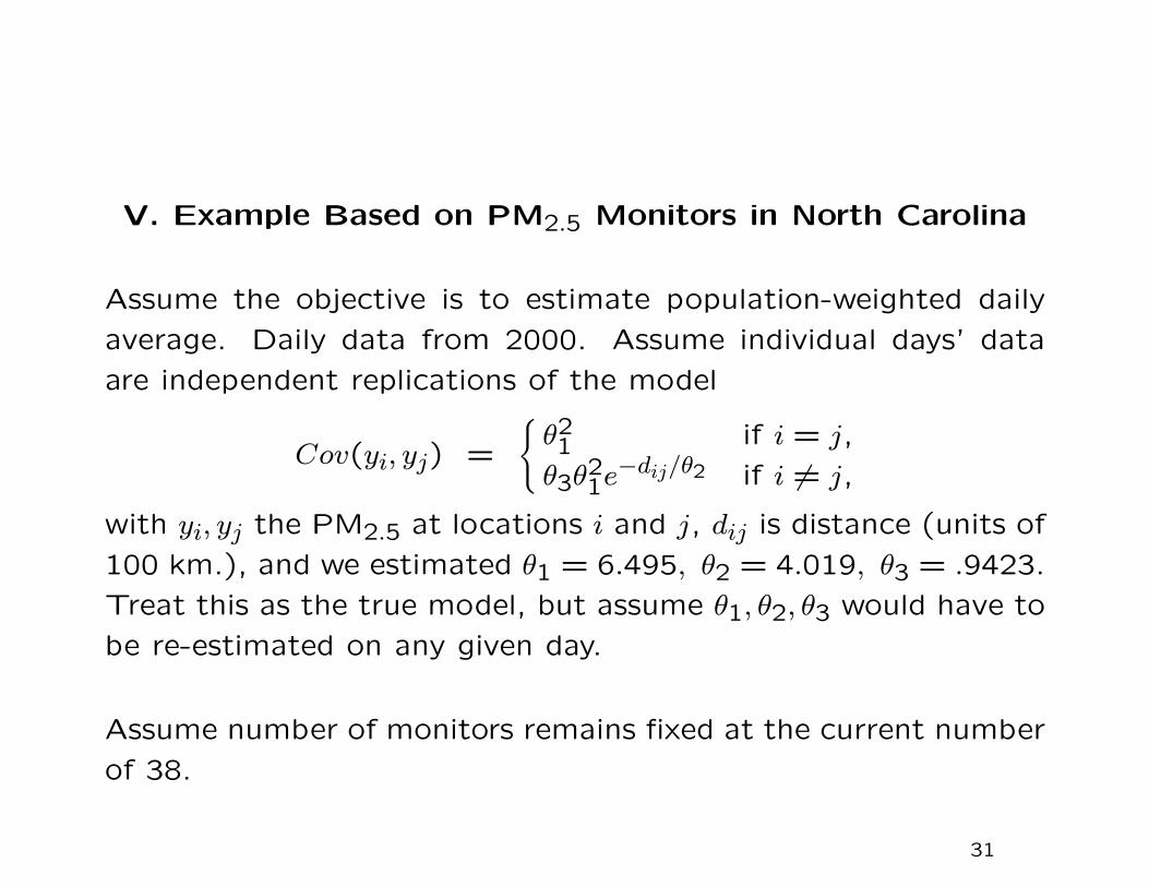
V. Example Based on PM2.5 Monitors in North Carolina

Assume the objective is to estimate population-weighted daily

average. Daily data from 2000. Assume individual days’ data

are independent replications of the model

Cov(yi, yj) =

{θ21 if i = j,

θ3θ21e−dij/θ2 if i 6= j,

with yi, yj the PM2.5 at locations i and j, dij is distance (units of

100 km.), and we estimated θ1 = 6.495, θ2 = 4.019, θ3 = .9423.

Treat this as the true model, but assume θ1, θ2, θ3 would have to

be re-estimated on any given day.

Assume number of monitors remains fixed at the current number

of 38.

31

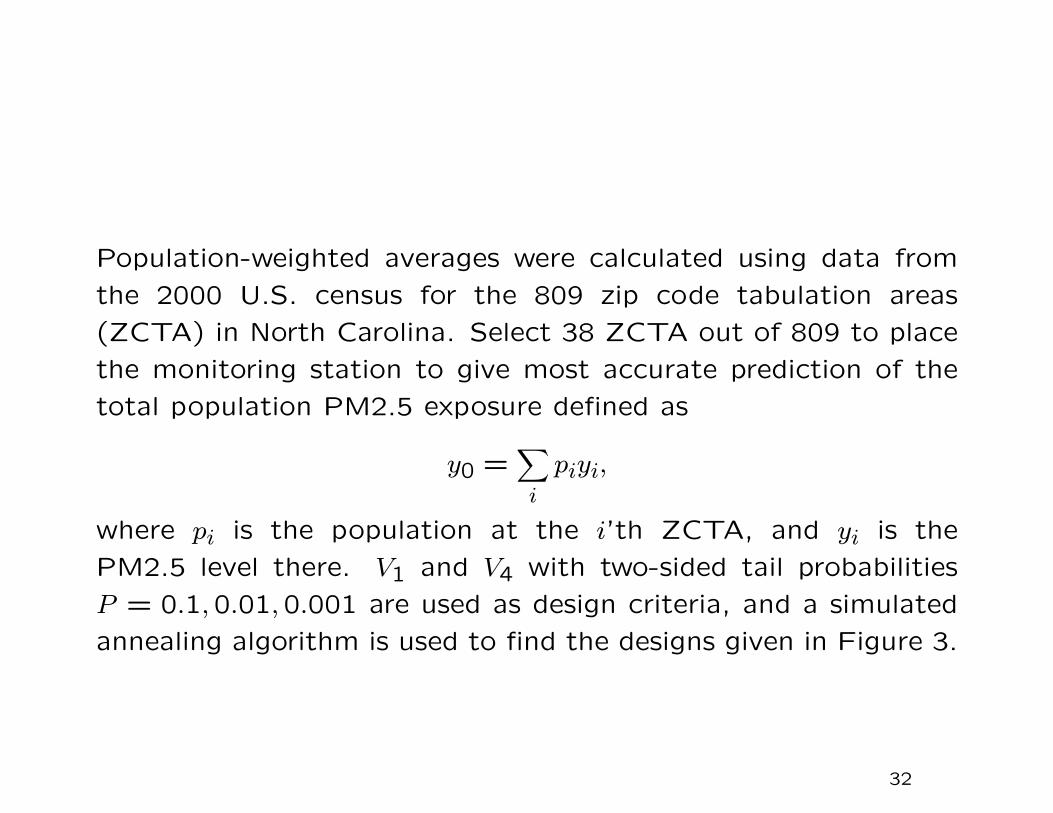
Population-weighted averages were calculated using data from

the 2000 U.S. census for the 809 zip code tabulation areas

(ZCTA) in North Carolina. Select 38 ZCTA out of 809 to place

the monitoring station to give most accurate prediction of the

total population PM2.5 exposure defined as

y0 =∑i

piyi,

where pi is the population at the i’th ZCTA, and yi is the

PM2.5 level there. V1 and V4 with two-sided tail probabilities

P = 0.1,0.01,0.001 are used as design criteria, and a simulated

annealing algorithm is used to find the designs given in Figure 3.

32

Point Predictor

o

o

oo o o

o

o

o

o

o

oo

o

oo

o

o

o

o

o

o

oo

oo

o

oo

oo

oo

o o

o

o

o

P=0.1

oo

o oo

o

o

o

o

o

oo

o

o

o

o

o

o

o o

o

o

oo

ooo

oo o o

o

o

o

o

o

o

o

P=0.01

ooo

o

o

o

oo

o

oo

o

o o

oo

o

o

o o

oo

o

o o

o

o

oo

o

o

o

oo

o

o

o

o

P=0.001

ooo

o

o

o

oo

o

oo

o

oo

oo

o

o

o o

oo

o

o o

o

o

oo

o

o

o

oo

o

o

o

o

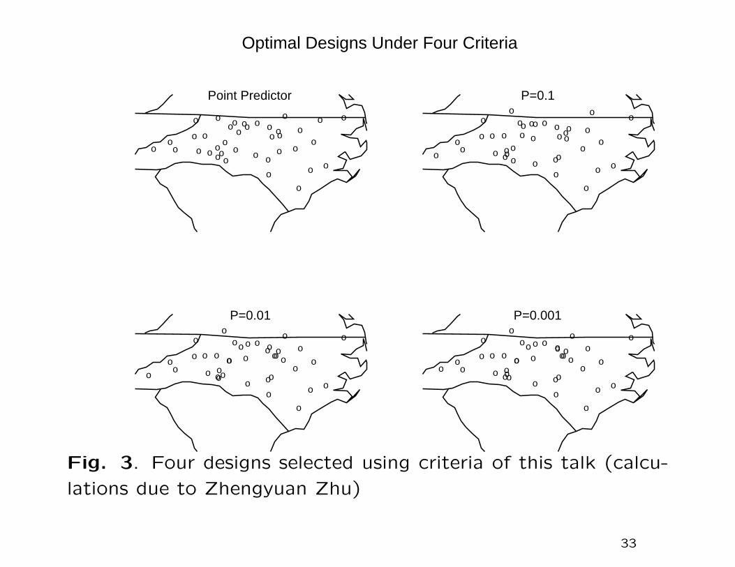
Optimal Designs Under Four Criteria

Fig. 3. Four designs selected using criteria of this talk (calcu-

lations due to Zhengyuan Zhu)

33

All four designs tend to place monitors in regions of high popu-

lation density (as does the current EPA network, Fig. 1) but it

is noticeable that the criterion V4, especially for smaller P , tends

to favor a network with clusters of nearby monitors, reflecting

the role such clusters play in ensuring good estimation of model

parameters.

34

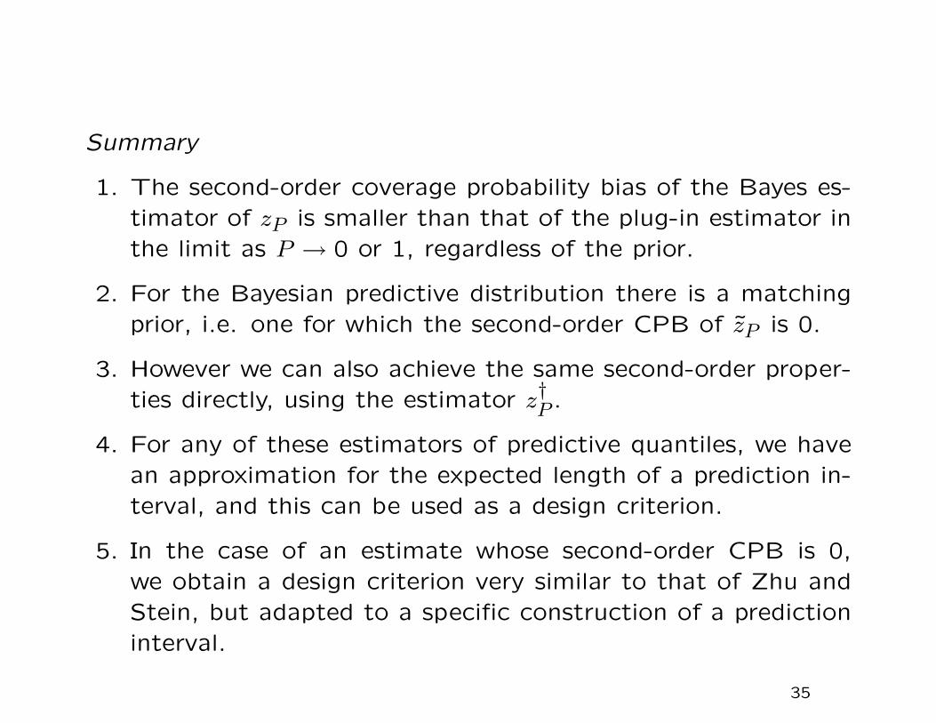
Summary

1. The second-order coverage probability bias of the Bayes es-timator of zP is smaller than that of the plug-in estimator inthe limit as P → 0 or 1, regardless of the prior.

2. For the Bayesian predictive distribution there is a matchingprior, i.e. one for which the second-order CPB of zP is 0.

3. However we can also achieve the same second-order proper-ties directly, using the estimator z†P .

4. For any of these estimators of predictive quantiles, we havean approximation for the expected length of a prediction in-terval, and this can be used as a design criterion.

5. In the case of an estimate whose second-order CPB is 0,we obtain a design criterion very similar to that of Zhu andStein, but adapted to a specific construction of a predictioninterval.

35