Embed Size (px)
Citation preview

7/28/2019 Kripke Recursion Theory
http://slidepdf.com/reader/full/kripke-recursion-theory 1/191
ELEMENTARY RECURSION THEORY AND ITS APPLICATIONS
TO FORMAL SYSTEMS
By Professor Saul Kripke
Department of Philosophy, Princeton University
Notes by Mario Gómez-Torrente,
revising and expanding notes by John Barker
Copyright © 1996 by Saul Kripke. Not for reproduction or quotation without express
permission of the author.
7/28/2019 Kripke Recursion Theory
http://slidepdf.com/reader/full/kripke-recursion-theory 2/191
Elementary Recursion Theory. Preliminary Version Copyright © 1995 by Saul Kripke
i
CONTENTS
Lecture I 1
First Order Languages / Eliminating Function Letters / Interpretations / The
Language of Arithmetic
Lecture II 8
The Language RE / The Intuitive Concept of Computability and its Formal
Counterparts / The Status of Church's Thesis
Lecture III 18
The Language Lim / Pairing Functions / Coding Finite Sequences
Lecture IV 27
Gödel Numbering / Identification / The Generated Sets Theorem / Exercises
Lecture V 36
Truth and Satisfaction in RE
Lecture VI 40
Truth and Satisfaction in RE (Continued) / Exercises
Lecture VII 49
The Enumeration Theorem. A Recursively Enumerable Set which is Not Recursive /
The Road from the Inconsistency of the Unrestricted Comprehension Principle to
the Gödel-Tarski Theorems
Lecture VIII 57
Many-one and One-one Reducibility / The Relation of Substitution / Deductive
Systems / The Narrow and Broad Languages of Arithmetic / The Theories Q and
PA / Exercises
Lecture IX 66
Cantor's Diagonal Principle / A First Version of Gödel's Theorem / More Versions
of Gödel's Theorem / Q is RE-Complete
Lecture X 73
True Theories are 1-1 Complete / Church's Theorem / Complete Theories are
Decidable / Replacing Truth by ω -Consistency / The Normal Form Theorem for RE
7/28/2019 Kripke Recursion Theory
http://slidepdf.com/reader/full/kripke-recursion-theory 3/191
Elementary Recursion Theory. Preliminary Version Copyright © 1995 by Saul Kripke
ii
/ Exercises
Lecture XI 81An Effective Form of Gödel's Theorem / Gödel's Original Proof / The
Uniformization Theorem for r.e. Relations / The Normal Form Theorem for Partial
Recursive Functions
Lecture XII 87
An Enumeration Theorem for Partial Recursive Functions / Reduction and
Separation / Functional Representability / Exercises
Lecture XIII 95
Languages with a Recursively Enumerable but Nonrecursive Set of Formulae / The
Smn Theorem / The Uniform Effective Form of Gödel's Theorem / The Second
Incompleteness Theorem
Lecture XIV 103
The Self-Reference Lemma / The Recursion Theorem / Exercises
Lecture XV 112
The Recursion Theorem with Parameters / Arbitrary Enumerations
Lecture XVI 116
The Tarski-Mostowski-Robinson Theorem / Exercises
Lecture XVII 124
The Evidence for Church's Thesis / Relative Recursiveness
Lecture XVIII 130
Recursive Union / Enumeration Operators / The Enumeration Operator Fixed-Point
Theorem / Exercises
Lecture XIX 138
The Enumeration Operator Fixed-Point Theorem (Continued) / The First and
Second Recursion Theorems / The Intuitive Reasons for Monotonicity and
Finiteness / Degrees of Unsolvability / The Jump Operator
Lecture XX 145
More on the Jump Operator / The Arithmetical Hierarchy / Exercises
7/28/2019 Kripke Recursion Theory
http://slidepdf.com/reader/full/kripke-recursion-theory 4/191
Elementary Recursion Theory. Preliminary Version Copyright © 1995 by Saul Kripke
iii
Lecture XXI 153
The Arithmetical Hierarchy and the Jump Hierarchy / Trial-and-Error Predicates /The Relativization Principle / A Refinement of the Gödel-Tarski Theorem
Lecture XXII 160
Theω -rule / The Analytical Hierarchy / Normal Form Theorems / Exercises
Lecture XXIII 167
Relative Σ's and Π's / Another Normal Form Theorem / Hyperarithmetical Sets
Lecture XXIV 173
Hyperarithmetical and ∆11 Sets / Borel Sets / Π1
1 Sets and Gödel's Theorem /
Arithmetical Truth is ∆11
Lecture XXV 182
The Baire Category Theorem / Incomparable Degrees / The Separation Theorem for
S11 Sets / Exercises
7/28/2019 Kripke Recursion Theory
http://slidepdf.com/reader/full/kripke-recursion-theory 5/191
Elementary Recursion Theory. Preliminary Version Copyright © 1996 by Saul Kripke
1
Lecture I
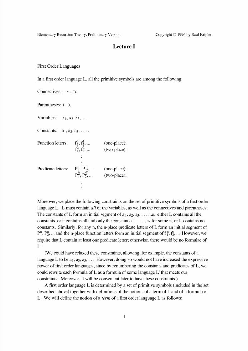
First Order Languages
In a first order language L, all the primitive symbols are among the following:
Connectives: ~ , ⊃.
Parentheses: ( , ).
Variables: x1, x2, x3, . . . .
Constants: a1, a2, a3, . . . .
Function letters: f 11, f 12, ... (one-place);
f 21, f 22, ... (two-place);
:
:
Predicate letters: P11, P 1
2, ... (one-place);
P21, P2
2, ... (two-place);
: :
Moreover, we place the following constraints on the set of primitive symbols of a first order
language L. L must contain all of the variables, as well as the connectives and parentheses.
The constants of L form an initial segment of a1, a2, a3, . . ., i.e., either L contains all the
constants, or it contains all and only the constants a1, . . ., an for some n, or L contains no
constants. Similarly, for any n, the n-place predicate letters of L form an initial segment of
Pn1, Pn
2, ... and the n-place function letters form an initial segment of f n1, f n2, ... However, we
require that L contain at least one predicate letter; otherwise, there would be no formulae of
L.(We could have relaxed these constraints, allowing, for example, the constants of a
language L to be a1, a3, a5, . . . However, doing so would not have increased the expressive
power of first order languages, since by renumbering the constants and predicates of L, we
could rewrite each formula of L as a formula of some language L' that meets our
constraints. Moreover, it will be convenient later to have these constraints.)
A first order language L is determined by a set of primitive symbols (included in the set
described above) together with definitions of the notions of a term of L and of a formula of
L. We will define the notion of a term of a first order language L as follows:
7/28/2019 Kripke Recursion Theory
http://slidepdf.com/reader/full/kripke-recursion-theory 6/191
Elementary Recursion Theory. Preliminary Version Copyright © 1996 by Saul Kripke
2
(i) Variables and constants of L are terms of L.
(ii) If t1, ..., t
nare terms of L and f n
iis a function letter of L, then f n
it1...t
nis a term of L.
(iii) The terms of L are only those things generated by clauses (i) and (ii).
Note that clause (iii) (the “extremal clause”) needs to be made more rigorous; we shall
make it so later on in the course.
An atomic formula of L is an expression of the form Pni t1...tn, where Pn
i is a predicate
letter of L and t1, ..., tn are terms of L. Finally, we define formula of L as follows:
(i) An atomic formula of L is a formula of L.
(ii) If A is a formula of L, then so is ~A.
(iii) If A and B are formulae of L, then (A⊃ B) is a formula of L.(iv) If A is a formula of L, then for any i, (xi) A is a formula of L.
(v) The formulae of L are only those things that are required to be so by clauses (i)-
(iv).
Here, as elsewhere, we use 'A', 'B', etc. to range over formulae.
Let xi be a variable and suppose that (xi)B is a formula which is a part of a formula A.
Then B is called the scope of the particular occurrence of the quantifier (xi) in A. An
occurrence of a variable xi in A is bound if it falls within the scope of an occurrence of the
quantifier (xi), or if it occurs inside the quantifier (xi) itself; and otherwise it is free. A
sentence (or closed formula) of L is a formula of L in which all the occurrences of variables
are bound.
Note that our definition of formula allows a quantifier (xi) to occur within the scope of
another occurrence of the same quantifier (xi), e.g. (x1)(P11x1 ⊃ (x1) P1
2x1). This is a bit
hard to read, but is equivalent to (x1)(P11x1 ⊃ (x2) P1
2x2). Formulae of this kind could be
excluded from first order languages; this could be done without loss of expressive power,
for example, by changing our clause (iv) in the definition of formula to a clause like:
(iv') If A is a formula of L, then for any i, (xi) A is a formula of L, provided that (xi)
does not occur in A.
(We may call the restriction in (iv') the “nested quantifier restriction”). Our definition of
formula also allows a variable to occur both free and bound within a single formula; for
example, P11x1 ⊃ (x1) P1
2x1 is a well formed formula in a language containing P11 and P1
2. A
restriction excluding this kind of formulae could also be put in, again without loss of
expressive power in the resulting languages. The two restrictions mentioned were adopted
by Hilbert and Ackermann, but it is now common usage not to impose them in the definition
of formula of a first order language. We will follow established usage, not imposing the
7/28/2019 Kripke Recursion Theory
http://slidepdf.com/reader/full/kripke-recursion-theory 7/191
Elementary Recursion Theory. Preliminary Version Copyright © 1996 by Saul Kripke
3
restrictions, although imposing them might have some advantages and no important
disadvantadge.
We have described our official notation; however, we shall often use an unofficial
notation. For example, we shall often use 'x', 'y', 'z', etc. for variables, while officially we
should use 'x1', 'x2', etc. A similar remark applies to predicates, constants, and function
letters. We shall also adopt the following unofficial abbreviations:
(A ∨ B) for (~A ⊃ B);
(A ∧ B) for ~(A ⊃ ~B);
(A ≡ B) for ((A ⊃ B) ∧ (B ⊃ A));
(∃xi) A for ~(xi) ~A.
Finally, we shall often omit parentheses when doing so will not cause confusion; inparticular, outermost parentheses may usually be omitted (e.g. writing A ⊃ B for (A ⊃ B)).
It is important to have parentheses in our official notation, however, since they serve the
important function of disambiguating formulae. For example, if we did not have
parentheses (or some equivalent) we would have no way of distinguishing the two readings
of A⊃ B ⊃ C, viz. (A ⊃ (B⊃ C)) and ((A ⊃ B)⊃ C). Strictly speaking, we ought to prove
that our official use of parentheses successfully disambiguates formulae. (Church proves
this with respect to his own use of parentheses in his Introduction to Mathematical Logic.)
Eliminating Function Letters
In principle, we are allowing function letters to occur in our languages. In fact, in view of a
famous discovery of Russell, this is unnecessary: if we had excluded function letters, we
would not have decreased the expressive power of first order languages. This is because we
can eliminate function letters from a formula by introducing a new n+1-place predicate letter
for each n-place function letter in the formula. Let us start with the simplest case. Let f be
an n-place function letter, and let F be a new n+1-place predicate letter. We can then rewrite
f(x1, ..., xn) = y
as
F(x1, ..., xn, y).
If P is a one-place predicate letter, we can then rewrite
P(f(x1, ..., xn))
7/28/2019 Kripke Recursion Theory
http://slidepdf.com/reader/full/kripke-recursion-theory 8/191
Elementary Recursion Theory. Preliminary Version Copyright © 1996 by Saul Kripke
4
as
(∃y) (F(x1, ..., xn, y) ∧ P(y)).
The general situation is more complicated, because formulae can contain complex terms like
f(g(x)); we must rewrite the formula f(g(x)) = y as (∃z) (G(x, z) ∧ F(z, y)). By repeated
applications of Russell's trick, we can rewrite all formulae of the form t = x, where t is a
term. We can then rewrite all formulae, by first rewriting
A(t1, ..., tn)
as
(∃x1)...(∃xn) (x1 = t1 ∧ ... ∧ xn = tn ∧ A(x1, ..., xn)),
and finally eliminating the function letters from the formulae xi = ti.
Note that we have two different ways of rewriting the negation of a formula A(t1,...,tn).
We can either simply negate the rewritten version of A(t1, ..., tn):
~(∃x1)...(∃xn) (x1 = t1 ∧ ... ∧ xn = tn ∧ A(x1, ..., xn));
or we can rewrite it as
(∃x1)...(∃xn) (x1 = t1 ∧ ... ∧ xn = tn ∧ ~A(x1, ..., xn)).
Both versions are equivalent. Finally, we can eliminate constants in just the same way we
eliminated function letters, since x = ai can be rewritten P(x) for a new unary predicate P.
Interpretations
By an interpretation of a first order language L (or a model of L, or a structure appropriate
for L), we mean a pair <D, F>, where D (the domain) is a nonempty set, and F is a function
that assigns appropriate objects to the constants, function letters and predicate letters of L.
Specifically,
- F assigns to each constant of L an element of D;
- F assigns to each n-place function letter an n-place function with domain Dn and
range included in D; and
7/28/2019 Kripke Recursion Theory
http://slidepdf.com/reader/full/kripke-recursion-theory 9/191
Elementary Recursion Theory. Preliminary Version Copyright © 1996 by Saul Kripke
5
- F assigns to each n-place predicate letter of L an n-place relation on D (i.e., a subset
of Dn).
Let I = <D, F> be an interpretation of a first order language L. An assignment in I is a
function whose domain is a subset of the set of variables of L and whose range is a subset
of D (i.e., an assignment that maps some, possibly all, variables into elements of D). We
now define, for given I, and for all terms t of L and assignments s in I, the function Den(t,s)
(the denotation (in I) of a term t with respect to an assignment s (in I)), that (when defined)
takes a term and an assignment into an element of D, as follows:
(i) if t is a constant, Den(t, s)=F(t);
(ii) if t is a variable and s(t) is defined, Den(t, s)=s(t); if s(t) is undefined, Den(t, s) is
also undefined;(iii) if t is a term of the form f
n
i(t1, ..., tn) and Den(t j,s)=b j (for j = 1, ..., n), then Den(t,
s)=F(f n
i)(b1, ..., bn); if Den(t j,s) is undefined for some j≤n, then Den(t,s) is also
undefined.
Let us say that an assignment s is sufficient for a formula A if and only if it makes the
denotations of all terms in A defined, if and only if it is defined for every variable occurring
free in A (thus, note that all assignments, including the empty one, are sufficient for a
sentence). We say that an assignment s in I satisfies (in I) a formula A of L just in case
(i) A is an atomic formula Pn
i(t1, ..., tn), s is sufficient for A and
<Den(t1,s),...,Den(tn,s)> ∈ F(Pn
i); or
(ii) A is ~B, s is sufficient for B but s does not satisfy B; or
(iii) A is (B ⊃ C), s is sufficient for B and C and either s does not satisfy B or s
satisfies C; or
(iv) A is (xi)B, s is sufficient for A and for every s' that is sufficient for B and such
that for all j≠i, s'(x j)=s(x j), s' satisfies B.
We also say that a formula A is true (in an interpretation I) with respect to an assignment s(in I) iff A is satisfied (in I) by s; if s is sufficient for A and A is not true with respect to s,
we say that A is false with respect to s.
If A is a sentence, we say that A is true in I iff all assignments in I satisfy A (or, what is
equivalent, iff at least one assignment in I satisfies A).
We say that a formula A of L is valid iff for every interpretation I and all assignments s
in I, A is true (in I) with respect to s (we also say, for languages L containing P21, that a
formula A of L is valid in the logic with identity iff for every interpretation I=<D,F> where
F(P21) is the identity relation on D, and all assignments s in I, A is true (in I) with respect to
7/28/2019 Kripke Recursion Theory
http://slidepdf.com/reader/full/kripke-recursion-theory 10/191
Elementary Recursion Theory. Preliminary Version Copyright © 1996 by Saul Kripke
6
s). More generally, we say that A is a consequence of a set Γ of formulas of L iff for every
interpretation I and every assignment s in I, if all the formulas of Γ are true (in I) with
respect to s, then A is true (in I) with respect to s. Note that a sentence is valid iff it is truein all its interpretations iff it is a consequence of the empty set. We say that a formula A is
satisfiable iff for some interpretation I, A is true (in I) with respect to some assignment in I.
A sentence is satisfiable iff it is true in some interpretation.
For the following definitions, let an interpretation I=<D,F> be taken as fixed. If A is a
formula whose only free variables are x1, ..., xn, then we say that the n-tuple <a1, ..., an>
(∈Dn) satisfies A (in I) just in case A is satisfied by an assignment s (in I), where s(xi) = ai
for i = 1, ..., n. (In the case n = 1, we say that a satisfies A just in case the 1-tuple <a> does.)
We say that A defines (in I) the relation R (⊆Dn) iff R={<b1, ..., bn>: <b1,...,bn> satisfies
A}. An n-place relation R (⊆Dn) is definable (in I) in L iff there is a formula A of L whose
only free variables are x1, ..., xn, and such that A defines R (in I). Similarly, if t is a termwhose free variables are x1, ..., xn, then we say that t defines the function h, where h(a1, ...,
an) = b just in case Den(t,s)=b for some assignment s such that s(xi) = ai. (So officially
formulae and terms only define relations and functions when their free variables are x1, ...,
xn for some n; in practice we shall ignore this, since any formula can be rewritten so that its
free variables form an initial segment of all the variables.)
The Language of Arithmetic
We now give a specific example of a first order language, along with its standard or
intended interpretation. The language of arithmetic contains one constant a1, one function
letter f 11, one 2-place predicate letter P21, and two 3-place predicate letters P3
1, and P32. The
standard interpretation of this language is <N, F> where N is the set {0, 1, 2, ...} of natural
numbers, and where
F(a1) = 0;
F(f 11) = the successor function s(x) = x+1;
F(P21) = the identity relation {<x, y>: x = y};
F(P31) = {<x, y, z>: x + y = z}, the graph of the addition function;
F(P32) = {<x, y, z>: x.y = z}, the graph of the multiplication function.
We also have an unofficial notation: we write
0 for a1;
x' for f 11x;
x = y for P21xy;
A(x, y, z) for P31xyz;
7/28/2019 Kripke Recursion Theory
http://slidepdf.com/reader/full/kripke-recursion-theory 11/191
Elementary Recursion Theory. Preliminary Version Copyright © 1996 by Saul Kripke
7
M(x, y, z) for P32xyz.
This presentation of the language of arithmetic is rather atypical, since we use a functionletter for successor but we use predicates for addition and multiplication. Note, however, that
formulae of a language involving function letters for addition and multiplication instead of
the corresponding predicate letters could be rewritten as formulae of the language of
arithmetic via Russell’s trick.
A numeral is a term of the form 0'...', i.e. the constant 0 followed by zero or more
successor function signs. The numeral for a number n is zero followed by n successor
function signs; we shall use the notation 0(n) for the numeral for n (note that ‘n’ is not a
variable of our formal system, but a variable of our informal talk). It may be noted that the
only terms of the language of arithmetic, as we have set it up, are the numerals and
expressions of the form xi'...'.
Finally, note that for the language of arithmetic, we can define satisfaction in terms of
truth and substitution. This is because a k-tuple <n1, ..., nk> of numbers satisfies A(x1, ...,
xk) just in case the sentence A(0(n1), ..., 0(nk)) is true (where A(0(n1), ..., 0(nk)) comes from A
by substituting the numeral 0(ni) for all of the free occurrences of the variable xi).
7/28/2019 Kripke Recursion Theory
http://slidepdf.com/reader/full/kripke-recursion-theory 12/191
Elementary Recursion Theory. Preliminary Version Copyright © 1996 by Saul Kripke
8
Lecture II
The Language RE
We shall now introduce the language RE. This is not strictly speaking a first order
language, in the sense just defined. However, it can be regarded as a fragment of the first
order language of arithmetic.
In RE, the symbols ∧ and∨ are the primitive connectives rather than ~ and ⊃. RE
further contains the quantifier symbol ∃ and the symbol < as primitive. The terms and
atomic formulae of RE are those of the language of arithmetic as presented above. Then the
notion of formula of RE is defined as follows:
(i) An atomic formula of RE is a formula.
(ii) If A and B are formulae, so are (A ∧ B) and (A ∨ B).
(iii) If t is a term not containing the variable xi, and A is a formula, then (∃xi) A and (xi
< t) A are formulae.
(iv) Only those things generated by the previous clauses are formulae.
The intended interpretation of RE is the same as the intended interpretation of the first
order language of arithmetic (it is the same pair <D,F>). Such notions as truth and
satisfaction for formulae of RE and definability by formulae of RE are defined in a way
similar to that in which they would be defined for the language of arithmetic using our
general definitions of truth and satisfaction; in the appropriate clause, the quantifier (xi < t)
is intuitively interpreted as "for all xi less than t..." (it is a so called “bounded universal
quantifier”).
Note that RE does not contain negation, the conditional or unbounded universal
quantification. These are not definable in terms of the primitive symbols of RE. The
restriction on the term t of (xi < t) in clause (iii) above is necessary if we are to exclude
unbounded universal quantification from RE, because (xi < xi') B is equivalent to (xi) B.
The Intuitive Concept of Computability and its Formal Counterparts
The importance of the language RE lies in the fact that with its help we will offer a definition
that will try to capture the intuitive concept of computability. We call an n-place relation on
the set of natural numbers computable if there is an effective procedure which, when given
an arbitrary n-tuple as input, will in a finite time yield as output 'yes' or 'no' as the n-tuple is
or isn't in the relation. We call an n-place relation semi-computable if there is an effective
7/28/2019 Kripke Recursion Theory
http://slidepdf.com/reader/full/kripke-recursion-theory 13/191
Elementary Recursion Theory. Preliminary Version Copyright © 1996 by Saul Kripke
9
procedure such that, when given an n-tuple which is in the relation as input, it eventually
yields the output 'yes', and which when given an n-tuple which is not in the relation as input,
does not eventually yield the output 'yes'. We do not require the procedure to eventually
yield the output 'no' in this case. An n-place total function φ is called computable if there is
an effective procedure that, given an n-tuple <p1,...,pn> as input, eventually yields φ(p1,...,pn)
as output (unless otherwise noted, an n-place function is defined for all n-tuples of natural
numbers (or all natural numbers if n = 1) —this is what it means for it to be total; and only
takes natural numbers as values.)
It is important to note that we place no time limit on the length of computation for a
given input, as long as the computation takes place within a finite amount of time. If we
required there to be a time limit which could be effectively determined from the input, then
the notions of computability and semi-computability would collapse. For let S be a semi-
computable set, and let P be a semi-computation procedure for S. Then we could find acomputation procedure for S as follows. Set P running on input x, and determine a time
limit L from x. If x∈ S, then P will halt sometime before the limit L. If we reach the limit
L and P has not halted, then we will know that x ∉ P. So as soon as P halts or we reach L,
we give an output 'yes' or 'no' as P has or hasn't halted. We will see later in the course,
however, that the most important basic result of recursion theory is that the unrestricted
notions of computability and semi-computability do not coincide: there are semi-computable
sets and relations that are not computable.
The following, however, is true (the complement of an n-place relation R (-R) is the
collection of n-tuples of natural numbers not in R):
Theorem: A set S (or relation R) is computable iff S (R) and its complement are semi-
computable.
Proof: If a set S is computable, there is a computation procedure P for S. P will also be a
semi-computation procedure for S. To semi-compute the complement of S, simply follow
the procedure of changing a ‘no’ delivered by P to a ‘yes’. Now suppose we have semi-
computation procedures for both S and its complement. To compute whether a number n is
in S, run simultaneously the two semi-computation procedures on n. If the semi-
computation procedure for S delivers a ‘yes’, the answer is yes; if the semi-computation
procedure for -S delivers a ‘yes’, the answer is no.
We intend to give formal definitions of the intuitive notions of computable set and
relation, semi-computable set and relation, and computable function. Formal definitions of
these notions were offered for the first time in the thirties. The closest in spirit to the ones
that will be developed here were based on the formal notion of λ -definable function
presented by Church. He invented a formalism that he called ‘λ -calculus’, introduced the
notion of a function definable in this calculus (a λ -definable function), and put forward the
thesis that the computable functions are exactly the λ -definable functions. This is Church’s
7/28/2019 Kripke Recursion Theory
http://slidepdf.com/reader/full/kripke-recursion-theory 14/191
Elementary Recursion Theory. Preliminary Version Copyright © 1996 by Saul Kripke
10
thesis in its original form. It states that a certain formal concept correctly captures a certain
intuitive concept.
Our own approach to recursion theory will be based on the following form of Church’s
thesis:
Church’s Thesis: A set S (or relation R) is semi-computable iff S (R) is definable in the
language RE.
We also call the relations definable in RE recursively enumerable (or r.e.). Given our
previous theorem, we can define a set or relation to be recursive if both it and its
complement are r.e.
Our version of Church's Thesis implies that the recursive sets and relations are precisely
the computable sets and relations. To see this, suppose that a set S is computable. Then, bythe above theorem, S and its complement are semi-computable, and hence by Church’s
Thesis, both are r.e.; so S is recursive. Conversely, suppose S is recursive. Then S and -S
are both r.e., and therefore by Church's Thesis both are semi-computable. Then by the
above theorem, S is computable.
The following theorem will be of interest for giving a formal definition of the remaining
intuitive notion of computable function:
Theorem: A total function φ(m1,...,mn) is computable iff the n+1 place relation
φ(m1,...,mn)=p is semi-computable iff the n+1 place relation φ(m1,...,mn)=p is computable.
Proof: If φ(m1,...,mn) is computable, the following is a procedure that computes (and hence
also semi-computes) the n+1 place relation φ(m1,...,mn)=p. Given an input <p1,...,pn,p>,
compute φ(p1,...,pn). If φ(p1,...,pn)=p, the answer is yes; if φ(p1,...,pn)≠p, the answer is no.
Now suppose that the n+1 place relation φ(m1,...,mn)=p is semi-computable (thus the
following would still follow under the assumption that it is computable); then to compute
φ(p1,...,pn), run the semi-computation procedure on sufficient n+1 tuples of the form
<p1,...,pn,m>, via some time-sharing trick. For example, run five steps of the semi-
computation procedure on <p1,...,pn,0>, then ten steps on <p1,...,pn,0> and <p1,...,pn,1>, and
so on, until you get the n+1 tuple <p1,...,pn,p> for which the ‘yes’ answer comes up. And
then give as output p.
A partial function is a function defined on a subset of the natural numbers which need
not be the set of all natural numbers. We call an n-place partial function partial computable
iff there is a procedure which delivers φ(p1,...,pn) as output when φ is defined for the
argument tuple <p1,...,pn>, and that does not deliver any output if φ is undefined for the
argument tuple <p1,...,pn>. The following result, partially analogous to the above, still holds:
Theorem: A function φ(m1,...,mn) is partial computable iff the n+1 relation φ(m1,...,mn)=p
7/28/2019 Kripke Recursion Theory
http://slidepdf.com/reader/full/kripke-recursion-theory 15/191
Elementary Recursion Theory. Preliminary Version Copyright © 1996 by Saul Kripke
11
is semi-computable.
Proof: Suppose φ(m1,...,mn) is partial computable; then the following is a semi-computation
procedure for the n+1 relation φ(m1,...,m
n)=p: given an argument tuple <p
1,...,p
n,p>, apply
the partial computation procedure to <p1,...,pn>; if and only if it eventually delivers p as
output, the answer is yes. Now suppose that the n+1 relation φ(m1,...,mn)=p is semi-
computable. Then the following is a partial computation procedure for φ(m1,...,mn). Given
an input <p1,...,pn>, run the semi-computation procedure on n+1 tuples of the form
<p1,...,pn,m>, via some time-sharing trick. For example, run five steps of the semi-
computation procedure on <p1,...,pn,0>, then ten steps on <p1,...,pn,0> and <p1,...,pn,1>, and
so on. If you get an n+1 tuple <p1,...,pn,p> for which the ‘yes’ answer comes up, then give
as output p.
But it is not the case anymore that a function φ(m1,...,mn) is partial computable iff then+1 relation φ(m1,...,mn)=p is computable. There is no guarantee that a partial computation
procedure will provide a computation procedure for the relation φ(m1,...,mn)=p; if φ is
undefined for <p1,...,pn>, the partial computation procedure will never deliver an output, but
we may have no way of telling that it will not.
In view of these theorems, we now give formal definitions that intend to capture the
intuitive notions of computable function and partial computable function. An n-place partial
function is called partial recursive iff its graph is r.e. An n-place total function is called
total recursive (or simply recursive) iff its graph is r.e. Sometimes the expression ‘general
recursive’ is used instead of ‘total recursive’, but this is confusing, since the expression
‘general recursive’ was originally used not as opposed to ‘partial recursive’ but as opposed
to ‘primitive recursive’.
It might seem that we can avoid the use of partial functions entirely, say by replacing a
partial function φwith a total function ψ which agrees with φwherever φ is defined, and
which takes the value 0 where φ is undefined. Such a ψ would be a total extension of φ, i.e.
a total function which agrees with φwherever φ is defined. However, this will not work,
since there are some partial recursive functions which are not totally extendible, i.e. which
do not have any total extensions which are recursive functions. (We shall prove this later on
in the course.)
Our version of Church's Thesis implies that a function is computable iff it is recursive.To see this, suppose that φ is a computable function. Then, by one of the theorems above, its
graph is semi-computable, and so by Church’s Thesis, it is r.e., and so φ is recursive.
Conversely, suppose that φ is recursive. Then φ's graph is r.e., and by Church's Thesis it is
semi-computable; so by the same theorem, φ is computable.
Similarly, our version of Church’s Thesis implies that a function is partial computable
iff it is partial recursive.
We have the result that if a total function has a semi-computable graph, then it has a
computable graph. That means that the complement of the graph is also semi-computable.
7/28/2019 Kripke Recursion Theory
http://slidepdf.com/reader/full/kripke-recursion-theory 16/191
Elementary Recursion Theory. Preliminary Version Copyright © 1996 by Saul Kripke
12
We should therefore be able to show that the graph of a recursive function is also recursive.
In order to do this, suppose that φ is a recursive function, and let R be its graph. R is r.e., so
it is defined by some RE formula B(x1, ..., x
n, x
n+1). To show that R is recursive, we must
show that -R is r.e., i.e. that there is a formula of RE which defines -R. A natural attempt is
the formula
(∃xn+2)(B(x1, ..., xn, xn+2) ∧ xn+1 ≠ xn+2).
This does indeed define -R as is easily seen, but it is not a formula of RE, for its second
conjunct uses negation, and RE does not have a negation sign. However, we can fix this
problem if we can find a formula of RE that defines the nonidentity relation {<m,n>:m≠n}.
Let us define the formula
Less (x, y) =df. (∃z) A(x, z', y).
Less (x, y) defines the less-than relation {<m, n>: m < n}. We can now define inequality as
follows:
x ≠ y =df. Less(x, y) ∨ Less (y, x).
This completes the proof that the graph of a total recursive function is a recursive relation,
and also shows that the less-than and nonidentity relations are r.e., which will be useful in
the future.
While we have not introduced bounded existential quantification as a primitive notation
of RE, we can define it in RE, as follows:
(∃x < t) B =df. (∃x) (Less(x, t) ∧ B).
In practice, we shall often write 'x < y' for 'Less (x, y)'. However, it is important to
distinguish the defined symbol '<' from the primitive symbol '<' as it appears within the
bounded universal quantifier. We also define
(∃x ≤ t) B(x) =df. (∃x < t) B(x) ∨ B(t);
(x ≤ t) B(x) =df. (x < t) B(x) ∧ B(t).
The Status of Church's Thesis
Our form of Church's thesis is that the intuitive notion of semi-computability and the formal
notion of recursive enumerability coincide. That is, a set or relation is semi-computable iff it
7/28/2019 Kripke Recursion Theory
http://slidepdf.com/reader/full/kripke-recursion-theory 17/191
Elementary Recursion Theory. Preliminary Version Copyright © 1996 by Saul Kripke
13
is r.e. Schematically:
r.e. = semi-computable.
The usual form of Church's Thesis is: recursive = computable. But as we saw, our form of
Church's Thesis implies the usual form.
In some introductory textbooks on recursion theory Church's Thesis is assumed in
proofs, e.g. in proofs that a function is recursive that appeal to the existence of an effective
procedure (in the intuitive sense) that computes it. (Hartley Rogers' Theory of Recursive
Functions and Effective Computability is an example of this.) There are two advantages to
this approach. The first is that the proofs are intuitive and easier to grasp than very
“formal” proofs. The second is that it allows the student to cover relatively advanced
material fairly early on. The disadvantage is that, since Church's Thesis has not actuallybeen proved, the student never sees the proofs of certain fundamental theorems. We shall
therefore not assume Church's Thesis in our proofs that certain sets or relations are
recursive. (In practice, if a recursion theorist is given an informal effective procedure for
computing a function, he or she will regard it as proved that that function is recursive.
However, an experienced recursion theorist will easily be able to convert this proof into a
rigorous proof which makes no appeal whatsoever to Church's Thesis. So working
recursion theorists should not be regarded as appealing to Church's Thesis in the sense of
assuming an unproved conjecture. The beginning student, however, will not in general have
the wherewithal to convert informal procedures into rigorous proofs.)
Another usual standpoint in some presentations of recursion theory is that Church's
Thesis is not susceptible of proof or disproof, because the notion of recursiveness is a
precise mathematical notion and the notion of computability is an intuitive notion. Indeed,
it has not in fact been proved (although there is a lot of evidence for it), but in the author's
opinion, no one has shown that it is not susceptible of proof or disproof. Although the
notion of computability is not taken as primitive in standard formulations of mathematics,
say in set theory, it does have many intuitively obvious properties, some of which we have
just used in the proofs of perfectly rigorous theorems. Also, y = x! is evidently computable,
and so is z=xy (although it is not immediately obvious that these functions are recursive, as
we have defined these notions). So suppose it turned out that one of these functions wasnot recursive. That would be an absolute disproof of Church's Thesis. Years before the
birth of recursion theory a certain very wide class of computable functions was isolated, that
later would come to be referred to as the class of “primitive recursive” functions. In a
famous paper, Ackermann presented a function which was evidently computable (and which
is in fact recursive), but which was not primitive recursive. If someone had conjectured that
the computable functions are the primitive recursive functions, Ackermann’s function would
have provided an absolute disproof of that conjecture. (Later we will explain what is the
class of primitive recursive functions and we will define Ackermann’s function.) For
7/28/2019 Kripke Recursion Theory
http://slidepdf.com/reader/full/kripke-recursion-theory 18/191
Elementary Recursion Theory. Preliminary Version Copyright © 1996 by Saul Kripke
14
another example, note that the composition of two computable functions is intuitively
computable; so, if it turned out that the formal notion of recursiveness was not closed under
composition, this would show that Church’s Thesis is wrong.
Perhaps some authors acknowledge that Church's Thesis is open to absolute disproof,
as in the examples above, but claim that it is not open to proof. However, the conventional
argument for this goes on to say that since computability and semi-computability are merely
intuitive notions, not rigorous mathematical notions, a proof of Church's Thesis could not be
given. This position, however, is not consistent if the intuitive notions in question cannot be
used in rigorous mathematical arguments. Then a disproof of Church's Thesis would be
impossible also, for the same reason as a proof. In fact, suppose for example that we could
give a list of principles intuitively true of the computable functions and were able to prove
that the only class of functions with these properties was exactly the class of the recursive
functions. We would then have a proof of Church's Thesis. While this is in principlepossible, it has not yet been done (and it seems to be a very difficult task).
In any event, we can give a perfectly rigorous proof of one half of Church's thesis,
namely that every r.e relation (or set) is semi-computable.
Theorem: Every r.e. relation (or set) is semi-computable.
Proof: We show by induction on the complexity of formulae that for any formula B of RE,
the relation that B defines is semi-computable, from which it follows that all r.e. relations are
semi-computable. We give, for each formula B of RE, a procedure PB which is a semi-
computation of the relation defined by B.
If B is atomic, then it is easy to see that an appropriate PB exists; for example, if B is
the formula x1''' = x2', then PB is the following procedure: add 3 to the first input, then add
1 to the second input, and see if they are the same, and if they are, halt with output 'yes'.
If B is (C ∧ D), then PB is the following procedure: first run PC, and if it halts with
output 'yes', run PD; if that also halts, then halt with output 'yes'.
If B is (C ∨ D), then PB is as follows. Run PC and PD simultaneously via some time-
sharing trick. (For example, run 10 steps of PC, then 10 steps of PD, then 10 more steps of
PC, ....) As soon as one answers 'yes', then let PB halt with output 'yes'.
Suppose now that B is (y < t) C(x1, ..., xn, y). If t is a numeral 0(p), then <m1, ..., mn>
satisfies B just in case all of <m1, ..., mn, 0> through <m1, ..., mn, p-1> satisfy C, so run PC
on input <m1, ..., mn, 0>; if PC answers yes, run PC on input <m1, ..., mn, 1>, .... If you
reach p-1 and get an answer yes, then <m1, ..., mn> satisfies B, so halt with output 'yes'. If t
is a term xi'...', then the procedure is basically the same. Given an input which includes the
values m1, ..., mn of x1, ..., xn, as well as the value of xi, first calculate the value p of the term
t, and then run PC on <m1, ..., mn, 0> through <m1, ..., mn, p-1>, as above. So in either case,
an appropriate PB exists.
Finally, if B = (∃y) C(x1, ..., xn, y), then PC is as follows: given input <m1, ..., mn>, run
PC on <m1, ..., mn, k> simultaneously for all k and wait for PC to deliver 'yes' for some k.
7/28/2019 Kripke Recursion Theory
http://slidepdf.com/reader/full/kripke-recursion-theory 19/191
Elementary Recursion Theory. Preliminary Version Copyright © 1996 by Saul Kripke
15
Again, we use a time-sharing trick; for example: first run PC on <m1, ..., mn, 0> for 10
steps, then run PC on <m1, ..., mn, 0> and <m1, ..., mn, 1> for 20 steps each, then .... Thus,
an appropriate PB
exists in this case as well, which completes the proof.
This proof cannot be formalized in set theory, so in that sense the famous thesis of the
logicists that all mathematics can be done in set theory might be wrong. But a weaker thesis
that every intuitive mathematical notion can always be replaced by one definable in set
theory (and coextensive with it) might yet be right.
Kreisel's opinion—in a review—appears to be that computability is a legitimate primitive
only for intuitionistic mathematics. In classical mathematics it is not a primitive, although
( pace Kreisel) it could be taken to be one. In fact the above argument, that the recursive sets
are all computable, is not intuitionistically valid, because it assumes that a number will be
either in a set or in its complement. (If you don't know what intuitionism is, don't worry.)It is important to notice that recursiveness (and recursive enumerability) is a
property of a set, function or relation, not a description of a set, function or relation. In
other words, recursiveness is a property of extensions, not intensions. To say that a set is
r.e. is just to say that there exists a formula in RE which defines it, and to say that a set is
recursive is to say that there exists a pair of formulae in RE which define it and its
complement. But you don't necessarily have to know what these formulae are, contrary to
the point of view that would be taken on this by intuitionistic or constructivist
mathematicians. We might have a theory of recursive descriptions, but this would not be
conventional recursive function theory. So for example, we know that any finite set is
recursive; every finite set will be defined in RE by a formula of the form
x1=0(k1)∨...∨xn=0(kn), and its complement by a formula of the form
x1≠0(k1)∧...∧xn≠0(kn). But we may have no procedure for deciding whether something is
in a certain finite set or not - finding such a procedure might even be a famous unsolved
problem. Consider this example: let S = {n: at least n consecutive 7's appear in the decimal
expansion of π}. Now it's hard to say what particular n's are in S (it's known that at least
four consecutive 7's appear, but we certainly don't know the answer for numbers much
greater than this), but nonetheless S is recursive. For, if n∈ S then any number less than n
is also in S, so S will either be a finite initial segment of the natural numbers, or else it will
contain all the natural numbers. Either way, S is recursive.There is, however, an intensional version of Church’s Thesis that, although hard to state
in a rigorous fashion, seems to be true in practice: whenever we have an intuitive procedure
for semi-computing a set or relation, it can be “translated” into an appropriate formula of
the formalism RE, and this can be done in some sense effectively (the “translation” is
intuitively computable). This version of Church’s Thesis operates with the notion of
arbitrary descriptions of sets or relations (in English, or in mathematical notation, say),
which is somewhat vague. It would be good if a more rigorous statement of this version of
Church’s Thesis could be made.
7/28/2019 Kripke Recursion Theory
http://slidepdf.com/reader/full/kripke-recursion-theory 20/191
Elementary Recursion Theory. Preliminary Version Copyright © 1996 by Saul Kripke
16
The informal notion of computability we intend to study in this course is a notion
different from a notion of analog computability that might be studied in physics, and for
which there is no reason to believe that Church’s Thesis holds. It is not at all clear that every
function of natural numbers computable by a physical device, that can use analog properties
of physical concepts, is computable by a digital algorithm. There have been some
discussions of this matter in a few papers, although the ones known to the author are quite
complicated. Here we will make a few rather unsophisticated remarks.
There are certain numbers in physics known as universal constants. Some of these
numbers are given in terms of units of measure, an are different depending on the system of
units of measures adopted. Some other of these numbers, however, are not given in terms of
units of measure, for example, the electron-proton mass ratio; that is, the ratio of the mass of
an electron to the mass of a proton. We know that the electron-proton mass ratio is a
positive real number r less than 1 (the proton is heavier than the electron). Consider thefollowing function ψ : ψ (k) = the kth number in the decimal expansion of r. (There are two
ways of expanding finite decimals, with nines at the end or with zeros at the end; in case r is
finite, we arbitrarily stipulate that its expansion is with zeros at the end.) As far as I know,
nothing known in physics allows us to ascribe to r any mathematical properties (e.g., being
rational or irrational, being algebraic or transcendental, even being a finite or an infinite
decimal). Also, as far as I know, it is not known whether this number is recursive, or Turing
computable.
However, people do attempt to measure these constants. There might be problems in
carrying out the measurement to an arbitrary degree of accuracy. It might take longer and
longer to calculate each decimal place, it might take more and more energy, time might be
finite, etc. Nevertheless, let us abstract from all these difficulties, assuming, e.g., that time is
infinite. Then, as far as I can see, there is no reason to believe that there cannot be any
physical device that would actually calculate each decimal place of r. But this is not an
algorithm in the standard sense.ψ might even then be uncomputable in the standard sense.
Let us review another example. Consider some quantum mechanical process where we
can ask, e.g., whether a particle will be emitted by a certain source in the next second, or
hour, etc. According to current physics, this kind of thing is not a deterministic process, and
only relevant probabilities can be given that a particle will be emitted in the next second, say.
Suppose we set up the experiment in such a way that there is a probability of 1/2 for anemission to occur in the next second, starting at some second s0. We can then define a
function χ(k) = 1 if an emission occurs in sk, and = 0 if an emission does not occur in sk.
This is not a universally defined function like ψ , but if time goes on forever, this experiment
is a physical device that gives a universally defined function. There are only a denumerable
number of recursive functions (there are only countably many strings in RE, and hence only
countably many formulae). In terms of probability theory, for any infinite sequence such as
the one determined by χ there is a probability of 1 that it will lie outside any denumerable
set (or set of measure zero). So in a way we can say with certainty that χ, even though
7/28/2019 Kripke Recursion Theory
http://slidepdf.com/reader/full/kripke-recursion-theory 21/191
Elementary Recursion Theory. Preliminary Version Copyright © 1996 by Saul Kripke
17
“computable” by our physical device, is not recursive, or, equivalently, Turing computable.
(Of course, χ may turn out to be recursive if there is an underlying deterministic structure to
our experiment, but assuming quantum mechanics, there is not.) This example again
illustrates the fact that the concept of physical computability involved is not the informal
concept of computability referred to in Church’s Thesis.
7/28/2019 Kripke Recursion Theory
http://slidepdf.com/reader/full/kripke-recursion-theory 22/191
Elementary Recursion Theory. Preliminary Version Copyright © 1996 by Saul Kripke
18
Lecture III
The Language Lim
In the language RE, we do not have a negation operator. However, sometimes, the
complement of a relation definable by a formula of RE is definable in RE by means of some
trick. We have already seen that the relation defined by t1≠t2 (where t1, t2 are two terms of
RE) is definable in RE, and whenever B defines the graph of a total function, the
complement of this graph is definable.
In RE we also do not have the conditional. However, if A is a formula whose negation
is expressible in RE, say by a formula A* (notice that A need not be expressible in RE),then the conditional (A ⊃B) would be expressible by means of (A*∨B) (provided B is a
formula of RE); thus, for example, (t1=t2⊃B) is expressible in RE, since t1≠t2 is. So when
we use the conditional in our proofs by appeal to formulae of RE, we’ll have to make sure
that if a formula appears in the antecedent of a conditional, its negation is expressible in the
language. In fact, this requirement is too strong, since a formula appearing in the antecedent
of a conditional may appear without a negation sign in front of it when written out only in
terms of negation, conjunction and disjunction. Consider, for example, a formula
(A ⊃B) ⊃C,
in which the formula A appears as a part in the antecedent of a conditional. This conditional
is equivalent to
(~A∨B)⊃C,
and in turn to
~(~A∨B)∨C,
and to
(A∧~B)∨C.
In the last formula, in which only negation, conjunction and disjunction are used, A appears
purely positively, so it’s not necessary that its negation be expressible in RE in order for (A
⊃B) ⊃C to be expressible in RE.
A bit more rigorously, we give an inductive construction that determines when an
7/28/2019 Kripke Recursion Theory
http://slidepdf.com/reader/full/kripke-recursion-theory 23/191
Elementary Recursion Theory. Preliminary Version Copyright © 1996 by Saul Kripke
19
occurrence of a formula A in a formula F whose only connectives are ~ and ⊃ is positive or
negative: if A is F, A's occurrence in F is positive; if F is ~B, A's occurrence in F is negative
if it is positive in B, and vice versa; if F is (B⊃
C), an occurrence of A in B is negative if
positive in B, and vice versa, and an occurrence of A in C is positive if positive in C, and
negative if negative in C.
It follows from this that if an occurrence of a formula appears as a part in another
formula in an even number of antecedents (e.g., A in the formula of the example above), the
corresponding occurrence will be positive in an ultimately reduced formula employing only
negation, conjunction and disjunction. If an occurrence of a formula appears as a part in
another formula in an odd number of antecedents (e.g., B in the formula above), the
corresponding occurrence will appear with a negation sign in front of it in the ultimately
reduced formula (i.e., it will be negative) and we will have to make sure that the negated
formula is expressible in RE.In order to avoid some of these complications involved in working within RE, we will
now define a language in which we have unrestricted use of negation, but such that all the
relations definable in it will also be definable in RE. We will call this language Lim. Lim has
the same primitive symbols as RE, plus a symbol for negation (~). The terms and atomic
formulae of Lim are just those of RE. Then the notion of formula of Lim is defined as
follows:
(i) An atomic formula of Lim is a formula of Lim;
(ii) If A and B are formulae of Lim, so are ~A, (A∧ B) and (A ∨ B);
(iii) If t is a term not containing the variable xi, and A is a formula of Lim, then (∃xi<t))
A and (xi < t) A are formulae of Lim;
(iv) Only those things generated by the previous clauses are formulae.
Notice that in Lim we no longer have unbounded existential quantification, but only
bounded existential quantification. This is the price of having negation in Lim.
Lim is weaker than RE in the sense that any set or relation definable in Lim is also
definable in RE. This will mean that if we are careful to define a relation using only
bounded quantifiers, its complement will be definable in Lim, and hence in RE, and this will
show that the relation is recursive. Call two formulae with the same free variables equivalent just in case they define the same set or relation. (So closed formulae, i.e. sentences, are
equivalent just in case they have the same truth value.) To show that Lim is weaker than RE,
we prove the following
Theorem: Any formula of Lim is equivalent to some formula of RE.
Proof : We show by induction on the complexity of formulae that if B is a formula of Lim,
then both B and ~B are equivalent to formulae of RE. First, suppose B is atomic. B is then
a formula of RE, so obviously B is equivalent to some RE formula. Since inequality is an
7/28/2019 Kripke Recursion Theory
http://slidepdf.com/reader/full/kripke-recursion-theory 24/191
Elementary Recursion Theory. Preliminary Version Copyright © 1996 by Saul Kripke
20
r.e. relation and the complement of the graph of any recursive function is r.e., ~B is
equivalent to an RE formula. If B is ~C, then by inductive hypothesis C is equivalent to an
RE formula C* and ~C is equivalent to an RE formula C**; then B is equivalent to C**
and ~B (i.e., ~~C) is equivalent to C*. If B is (C ∧ D), then by the inductive hypothesis, C
and D are equivalent to RE formulae C* and D*, respectively, and ~C, ~D are equivalent to
RE formulae C** and D**, respectively. So B is equivalent to (C* ∧ D*), and ~B is
equivalent to (C** ∨ D**). Similarly, if B is (C ∨ D), then B and ~B are equivalent to (C*
∨ D*) and (C** ∧ D**), respectively. If B is (∃xi < t) C, then B is equivalent to (∃xi
)(Less(xi, t)∧C*), and ~B is equivalent to (xi < t) ~C and therefore to (xi < t) C**. Finally,
the case of bounded universal quantification is similar.
A set or relation definable in Lim is recursive: if B defines a set or relation in Lim, then
~B is a formula of Lim that defines its complement, and so by the foregoing theorem both itand its complement are r.e. (Once we have shown that not all r.e. sets are recursive, it will
follow that Lim is strictly weaker than RE, i.e. that not all sets and relations definable in RE
are definable in Lim.) Since negation is available in Lim, the conditional is also available, as
indeed are all truth-functional connectives. Because of this, showing that a set or relation is
definable in Lim is a particularly convenient way of showing that it is recursive; in general, if
you want to show that a set or relation is recursive, it is a good idea to show that it is
definable in Lim (if you can).
We can expand the language Lim by adding extra predicate letters and function letters
and interpreting them as recursive sets and relations and recursive functions. If we do so,
the resulting language will still be weaker than RE:
Theorem: Let Lim' be an expansion of Lim in which the extra predicates and function
letters are interpreted as recursive sets and relations and recursive functions. Then every
formula of Lim' is equivalent to some formula of RE.
Proof : As before, we show by induction on the complexity of formulae that each formula
of Lim' and its negation are equivalent to RE formulae. The proof is analogous to the proof
of the previous theorem. Before we begin the proof, let us note that every term of Lim'
stands for a recursive function; this is simply because the function letters of Lim' define
recursive functions, and the recursive functions are closed under composition. So if t is aterm of Lim', then both t = y and ~(t = y) define recursive relations and are therefore
equivalent to formulae of RE.
Suppose B is the atomic formula P(t1, ..., tn), where t1, ..., tn are terms of Lim' and P is a
predicate of Lim' defining the recursive relation R. Using Russell's trick, we see that B is
equivalent to (∃x1)...(∃xn)(t1 = x1 ∧ ... ∧ tn = xn ∧ P(x1, ..., xn)), where x1, ..., xn do not
occur in any of the terms t1, ..., tn. Letting Ci be an RE formula which defines the relation
defined by ti = xi, and letting D be an RE formula which defines the relation that P defines,
we see that B is equivalent to the RE formula (∃x1)...(∃xn)(C1(x1) ∧ ... Cn(xn) ∧ D(x1, ...,
7/28/2019 Kripke Recursion Theory
http://slidepdf.com/reader/full/kripke-recursion-theory 25/191
Elementary Recursion Theory. Preliminary Version Copyright © 1996 by Saul Kripke
21
xn)). To see that ~B is also equivalent to an RE formula, note that R is a recursive relation,
so its complement is definable in RE, and so the formula (∃x1)...(∃xn)(t1 = x1 ∧ ... ∧ tn = xn
∧ ~P(x1, ..., x
n)), which is equivalent to ~B, is also equivalent to an RE formula.
The proof is the same as the proof of the previous theorem in the cases of conjunction,
disjunction, and negation. In the cases of bounded quantification, we have to make a slight
adjustment, because the term t in (xi < t) B or (∃xi < t) B might contain new function letters.
Suppose B and ~B are equivalent to the RE formulae B* and B**, and let t = y be
equivalent to the RE formula C(y). Then (xi < t) B is equivalent to the RE formula (∃y)
(C(y) ∧ (xi < y) B*)), and ~(xi < t) B is equivalent to (∃xi < t) ~B, which is in turn
equivalent to the RE formula (∃y) (C(y) ∧ (∃xi < y) B**). The case of bounded existential
quantification is similar.
This fact will be useful, since in RE and Lim the only bounds we have for the boundedquantifiers are terms of the forms 0(n) and xi'...'. In expanded languages containing
function letters interpreted as recursive functions there will be other kinds of terms that can
serve as bounds for quantifiers in formulae of the language, without these formulae failing
to be expressible in RE.
There is a variant of Lim that should be mentioned because it will be useful in future
proofs. Lim+ is the language which is just like Lim except that it has function letters rather
than predicates for addition and multiplication. (So in particular, quantifiers in Lim+ can be
bounded by terms containing + and ..) It follows almost immediately from the previous
theorem that every formula of Lim+ is equivalent to some formula of RE. We call a set or
relation limited if it is definable in the language Lim+. We call it strictly limited if it is
definable in Lim.
Pairing Functions
We will define a pairing function on the natural numbers to be a dominating total binary
recursive function φ such that for all m1, m2, n1, n2, if φ(m1, m2) = φ(n1, n2) then m1 = n1
and m2 = n2 (that a binary function φ is dominating means that for all m, n, m≤φ(m, n) and
n≤φ(m, n)). Pairing functions allow us to code pairs of numbers as individual numbers,since if p is in the range of a pairing function φ, then there is exactly one pair (m, n) such
that φ(m, n) = p, so the constituents m and n of the pair that p codes are uniquely determined
by p alone.
We are interested in finding a pairing function. If we had one, that would show that the
theory of recursive functions in two variables essentially reduces to the theory of recursive
functions in one variable. This will be because it is easily proved that for all binary relations
R, if φ is a pairing function, R is recursive (r.e.) iff the set {φ(m, n): R(m, n)} is recursive
(r.e.). We are going to see that there are indeed pairing functions, so that there is no
7/28/2019 Kripke Recursion Theory
http://slidepdf.com/reader/full/kripke-recursion-theory 26/191
Elementary Recursion Theory. Preliminary Version Copyright © 1996 by Saul Kripke
22
essential difference between the theories of recursive binary relations and of recursive sets.
This is in contrast to the situation in the topologies of the real line and the plane. Cantor
discovered that there is a one-to-one function from the real line onto the plane. This result
was found to be surprising by Cantor himself and by others, since the difference between
the line and the plane seemed to lie in the fact that points in the plane could only be
specified or uniquely determined by means of pairs of real numbers, and Cantor’s result
seemed to imply that every point in the plane could be identified by a single real number.
But the real line and the plane are topologically distinct, that is, there is no homeomorphism
of the real line onto the plane, which means that they are essentially different topological
spaces. In fact, Brouwer proved a theorem from which the general result follows that there is
no homeomorphism between m-dimensional Euclidean space and n-dimensional Euclidean
space (for m ≠ n).
The following will be our pairing function. Let us define [x, y] to be (x+y)2+x. Thisfunction is evidently recursive, since it is limited, as it is defined by the Lim+ formula z = (x
+ y).(x + y) + x, and is clearly dominating. Let us show that it is a pairing function, that is,
that for all z, if z = [x, y] for some x and y, then x and y are uniquely determined. Let z =
(x+y)2+x. (x+y)2 is uniquely determined, and it is the greatest perfect square ≤ z: if it
weren't, then we would have (x + y + 1)2 ≤ z, but (x + y + 1)2 = (x + y)2 + 2x + 2y + 1 >
(x + y)2 + x = z. Let s=x+y, so that s2=(x+y)2. Since z>s2, we can put x=z-s2, which is
uniquely determined, and y=s-x=s-(z-s2), which is uniquely determined. This completes the
proof that [x,y] is a pairing function. Note that it is not onto, i.e. some numbers do not code
pairs of numbers. For our purposes this will not matter.
(The earliest mention of this pairing function known to the author is in Goodstein’s
Recursive Number Theory. Several years later, the same function was used by Quine, who
probably thought of it independently.)
Our pairing function can be extended to n-place relations. First, note that we can get a
recursive tripling function by letting [x, y, z] = [[x, y], z]. We can similarly get a recursive
n-tupling function, [m1, ..., mn], and we can prove an analogous result to the above in the
case of n-place relations: for all n-place relations R, if φ is a recursive n-tupling function, R
is recursive (r.e.) iff the set {φ(m1,...,mn): R(m1,...,mn)} is recursive (r.e.).
Our pairing function has recursive inverses, i.e. there are recursive functions K1 and K2
such that K1([x, y]) = x and K2([x, y]) = y for all x and y. When z does not code any pair,we could let K1 and K2 be undefined on z; here, however, we let K1 and K2 have the value 0
on z. (So we can regard z as coding the pair <0, 0>, though in fact z ≠ [0, 0].) Intuitively,
K1 and K2 are computable functions, and indeed they are recursive. To see this, note that
K1's graph is defined by the formula of Lim (∃y ≤ z) (z = [x, y]) ∨ (x = 0 ∧ ~(∃y ≤ z) (∃w
≤ z) z = [w, y]); similarly, K2's graph is defined by the formula of Lim (∃x ≤ z) (z = [x, y])
∨ (y = 0 ∧ ~(∃x ≤ z) (∃w ≤ z) z = [x, w]).
7/28/2019 Kripke Recursion Theory
http://slidepdf.com/reader/full/kripke-recursion-theory 27/191
Elementary Recursion Theory. Preliminary Version Copyright © 1996 by Saul Kripke
23
Coding Finite Sequences
We have seen that for any n, there is a recursive n-tupling function; or in other words,
we have a way of coding finite sequences of fixed length. Furthermore, all these n-tupling
functions have recursive inverses. This does not, however, give us a single, one-to-one
function for coding finite sequences of arbitrary length. One of the things Cantor showed is
that there is a one-to-one correspondence between the natural numbers and the set of finite
sequences of natural numbers, so a function with the relevant property does exist. What we
need to do, in addition, is to show that an effective way of assigning different numbers to
different sequences exists, and such that the decoding of the sequences from their codes can
be done also effectively.
A method of coding finite sequences of variable length, due to Gödel, consists in
assigning to an n-tuple <m1, ..., mn> the number k=2m1+1.3m2+1. ... .pnmn+1 as code(where p1=2 and pi+1=the first prime greater than pi). It is clear that k can be uniquely
decoded, since every number has a unique prime factorization, and intuitively the decoding
function is computable. If we had exponentiation as a primitive of RE, it would be quite
easy to see that the decoding function is recursive; but we do not have it as a primitive.
Although Gödel did not take exponentiation as primitive, he found a trick, using the Chinese
Remainder Theorem, for carrying out the above coding with only addition, multiplication
and successor as primitive. We could easily have taken exponentiation as a primitive — it is
not essential to recursion theory that the language of RE have only successor, addition and
multiplication as primitive and other operations as defined. If we had taken it as primitive,
our proof of the easy half of Church's thesis, i.e. that all r.e. relations are semi-computable,
would still have gone through, since exponentiation is clearly a computable function.
Similarly, we could have added to RE new variables to range over finite sets of numbers, or
over finite sequences. In fact, doing so might have saved us some time at the beginning of
the course. However, it is traditional since Gödel’s work to take quantification over
numbers, and successor, addition, and multiplication as primitive and to show how to define
the other operations in terms of them.
We will use a different procedure for coding finite sequences, the basic idea of which is
due to Quine. If you want to code the sequence <5, 4, 7>, why not use the number 547? In
general, a sequence of positive integers less than 10 can be coded by the number whosedecimal expansion is the sequence. Unfortunately, if you want to code sequences
containing numbers larger than or equal to 10, this won't quite work. (Also, if the first
element of a sequence <m1, ..., mn> is 0, its code will be the same as the code for the
sequence <m2, ..., mn>; this problem is relatively minor compared to the other). Of course, it
is always possible to use a larger base; if you use a number to code its base-100 expansion,
for example, then you can code sequences of numbers as large as 99. Still, this doesn't
provide a single method for coding sequences of arbitrary length.
To get around this, we shall use a modification of Quine's trick, due to the author. The

7/28/2019 Kripke Recursion Theory
http://slidepdf.com/reader/full/kripke-recursion-theory 28/191
Elementary Recursion Theory. Preliminary Version Copyright © 1996 by Saul Kripke
24
main idea is to use a variable base, so that a number may code a different sequence to a
different base. It also proves convenient in this treatment to use only prime bases. Another
feature of our treatment is that we will code finite sets first, rather than finite sequences; this
will mean that every finite set will have many different codes (thus, using base 10 only for
purposes of motivation, 547 and 745 would code the same set {4, 5, 7}). We will not allow
0 as the first digit of a code (in a base p) of a set, because otherwise 0 would be classified as
a member of the set, whether it was in it or not (of course, 0 will be allowed as an
intermediate or final digit).
Our basic idea is to let a number n code the set of all the numbers that appear as digits
in n's base-p expansion, for appropriate prime p. No single p will do for all sets, since for
any prime p, there is a finite set containing numbers larger than p, and which therefore
cannot be represented as a base-p numeral. However, in view of a famous theorem due to
Euclid, we can get around this.
Theorem (Euclid): There are infinitely many primes.
Proof . Let n be any number, and let's show that there are primes greater than n . n! + 1 is
either prime or composite. If it is prime, it is a prime greater than n. If it is composite, then
it has some prime factor p; but then p must be greater than n, since n!+1 is not divisible by
any prime less than or equal to n. Either way, there is a prime number greater than n; and
since n was arbitrary, there are arbitrarily large primes.
So for any finite set S of numbers, we can find a prime p greater than any element of S, and
a number n such that the digits of the base-p expansion of n are the elements of S. (To give
an example, consider the finite set {1, 2}. This will have as “codes” in base 3 the numbers
denoted by '12' and '21' in base 3 notation, that is, 5 and 7; it will have as “codes” in base 5
the numbers 7 and 11, etc.) We can then take [n, p] as a code of the set S (so, in the
example, [5,3], [7,3], [7,5] and [11,5] are all codes of {1,2}). In this fashion different finite
sets will never be assigned the same code. Further, from a code the numbers n and p are
uniquely determined and effectively recoverable, and from n and p the set S is determined
uniquely.
We will now show how to carry out our coding scheme in RE. To this effect, we will
show that a number of relations are definable in Lim or Lim+ (and hence not only r.e, butalso recursive). Before we begin, let us note that the relation of nonidentity is definable in
Lim and in Lim+, for we can define a formula Less*(x,y) equivalent to the formula
Less(x,y) of RE with only bounded quantification: Less*(x,y) =df. (∃z<y)(x+z'=y) (an even
simpler formula defining the less than relation in Lim and Lim+ would be (∃z<y)(x=z)).
Now, let's put
Pr (x) =df. x ≠ 0 ∧ x ≠ 0' ∧ (y ≤ x)(z ≤ x)(M(y,z,x)⊃(y=x∨z=x)).
7/28/2019 Kripke Recursion Theory
http://slidepdf.com/reader/full/kripke-recursion-theory 29/191
Elementary Recursion Theory. Preliminary Version Copyright © 1996 by Saul Kripke
25
Pr(x) defines the set of primes in Lim, as is easily seen. We want next to define the relation
w is a power of p, for prime numbers p. This is done by
Ppow (p, w) =df. Pr(p) ∧ w ≠ 0 ∧ (x ≤ w)(y ≤ w)((M(x,y,w) ∧ Pr(x)) ⊃ x = p).
Ppow (p, w) says that p is w's only prime factor, and that w ≠ 0; this only holds if w = pk
for some k and p is prime. Note that if p is not prime, then this trick won't work.
Next, we want to define a formula Digp (m, n, p), which holds iff m is a digit in the
base-p expansion of n and p is prime. How might we go about this? Let's use base 10
again for purposes of illustration. Suppose n > 0, and let d be any number < 10. If d is the
first digit of n's decimal expansion, then n = d.10k + y, for some k and some y < 10k, and
moreover d ≠ 0. (For example, 4587 = 4.103 + 587.) Conversely, if n = d.10k + y for
some k and some y < 10k and if d ≠ 0, then d is the initial digit of the decimal expansion of n. If d is an intermediate or final digit in n's decimal expansion, then n = x.10k+1 + d.10k +
y for some k, x and y with y < 10k and x ≠ 0, and conversely. (This works for final digits
because we can always take y = 0.) So if d < 10 and n ≠ 0, then d is a digit of n iff d is
either an initial digit or an intermediate or final digit, iff there exist x, k, and y with y < 10k
and such that either d ≠ 0 and n = d.10k + y, or x ≠ 0 and n = x.10k+1 + d.10k + y. If 10 ≤
d then d is not a digit of n's decimal expansion, and we allow 0 to occur in its own decimal
expansion. The restrictions d ≠ 0 and x ≠ 0 are necessary, since otherwise 0 would occur in
the decimal expansion of every number: 457 = 0.103 + 457 = 0.104 + 0.103 + 457; and if
we want to code any finite sets that do not have 0 as an element, we must prevent this.
Noting that none of this depends on the fact that the base 10 was used, and finding bounds
for our quantifiers, we can define a formula Digp*(m, n, p) in Lim+, which is true of m,n,p
iff m is a digit in the base-p expansion of n and p is prime:
Digp* (m, n, p) =df. { n≠0 ∧ m < p ∧
[[m ≠ 0 ∧ (∃w ≤ n)(∃z < w)(n = m.w + z ∧ Ppow (p, w))] ∨
(∃w ≤ n)(∃z1 ≤ n)(∃z2 < w)(z1 ≠ 0 ∧ n = z1.w.p + m.w + z2
∧ Ppow (p, w))]}
∨
(m = 0 ∧ n = 0 ∧ Pr(p)).
This formula mirrors the justification given above. However, much of it turns out to be
redundant. Specifically, the less complicated formula
Digp (m, n, p) =df. (n≠0 ∧ m < p ∧
(∃w ≤ n)(∃z1 ≤ n)(∃z2 < w)(n = z1.w.p + m.w + z2 ∧
Ppow (p, w))])

7/28/2019 Kripke Recursion Theory
http://slidepdf.com/reader/full/kripke-recursion-theory 30/191
Elementary Recursion Theory. Preliminary Version Copyright © 1996 by Saul Kripke
26
∨ (m = 0 ∧ n = 0∧ Pr(p))
is equivalent to Digp* (this remark is due to John Barker). To see this, suppose first thatDigp*(m,n,p), m<p and n≠0. Then n = z1.pk+1 + m.pk + z2 for some k, z1 and some z2 <
pk. This includes initial digits (let z1 = 0) and final digits (let z2 = 0). So Digp (m, n, p)
holds. Conversely, suppose Digp (m, n, p) holds, and assume that m<p and n≠0. Then n =
z1.pk+1 + m.pk + z2 for some k, z1 and some z2 < pk, and moreover pk ≤ n. If z1 > 0, then
m must be an intermediate or final digit of n, so suppose z1 = 0. Then m > 0: for if m = 0,
then n = 0.pk+1 + 0.pk + z2 = z2, but z2 < pk and pk ≤ n, and so n < n. So m must be the
first digit of n.
We can now define
x ∈ y =df. (∃n ≤ y)(∃p ≤ y)(y = [n, p] ∧ Digp (x, n, p)).
x ∈ y is true of two numbers a,b if b codes a finite set S and a is a member of S. Note that
Digp(m,n,p) and x ∈ y are formulae of Lim+. We could have carried out the construction
in Lim, but it would have been more tedious, and would not have had any particular
advantage for the purposes of this course.
There are two special cases we should check to make sure our coding scheme works:
namely, we should make sure that the sets {0} and Ø have codes. If y is not in the range of
our pairing function, then x ∈ y will be false for all x; so y will code Ø. And since Digp(0,
0, p) holds for any p, [0, p] codes the set {0}.
7/28/2019 Kripke Recursion Theory
http://slidepdf.com/reader/full/kripke-recursion-theory 31/191
Elementary Recursion Theory. Preliminary Version Copyright © 1996 by Saul Kripke
27
Lecture IV
Let us now note a few bounding tricks that will be useful in the future. The function z =
[x, y] is monotone in both variables: i.e. if x ≤ x1 and y ≤ y1 then [x, y] ≤ [x1, y1].
Moreover, x, y ≤ [x, y]. Finally, if n codes a set S, and x∈ S, then x ≤ n: if n codes S, then
n is [k, p] for some k and p, so k ≤ n; and x is a digit in k's base-p expansion, so x ≤ k. So
we can introduce some new bounded quantifiers into Lim+:
(x ∈ y) B =df. (x ≤ y) (x ∈ y ⊃ B);
(∃x ∈ y) B =df. (∃x ≤ y) (x ∈ y ∧ B).
Note also that if n codes a set S and S' ⊆ S, then there is an m ≤ n which codes S'. (This is
because, if the elements of S are the digits of the base-p expansion of k, then there is a
number j ≤ k such that the digits in j's base-p expansion are the elements of S'; since j ≤ k,
[j, p] ≤ [k, p] and [j, p] codes S'.) We can therefore define
x ⊆ y =df. (z ∈ x) z ∈ y;
(x ⊆ y) B =df. (x ≤ y) (x ⊆ y ⊃ B);
(∃x ⊆ y) B =df. (∃x ≤ y) (x ⊆ y ∧ B).
Now that we can code finite sets of numbers, it is easy to code finite sequences. For a
sequence <m1, ..., mn> is simply a function φ with domain {1, ..., n} and with φ(i) = mi; we
can identify functions with their graphs, which are relations, i.e. sets of ordered pairs, which
we can in turn identify with sets of numbers, since we can code up ordered pairs as
numbers. (So, for example, we can identify the sequence <7, 5, 10> with the set {[1, 7], [2,
5], [3, 10]}.) Finally, those sets can themselves be coded up as numbers. We define a
formula Seql (s, n) of Lim+ which holds just in case s codes a sequence of length n:
Seql (s, n) =df. (x ∈ s)(∃m1 ≤ s)(∃m2 ≤ s)(x = [m1, m2] ∧ m1 ≠ 0∧ m1 ≤ n) ∧(m1 ≤ s)(m2 ≤ s)(m3 ≤ s)(([m1, m2] ∈ s ∧ [m1, m3] ∈ s) ⊃ m2 = m3)
∧ (m1≤ n)(∃m2 ≤ s)(m1 ≠ 0 ⊃ [m1, m2] ∈ s).
The first conjunct simply says that every element of s is a pair whose first member is a
positive integer ≤ n; the second says that s is single valued, i.e. is (the graph of) a function;
and the third says that every positive integer ≤ n is in s's domain.
We can also define a formula Seq (s), which says that s codes a finite sequence of some
length or other:
7/28/2019 Kripke Recursion Theory
http://slidepdf.com/reader/full/kripke-recursion-theory 32/191
Elementary Recursion Theory. Preliminary Version Copyright © 1996 by Saul Kripke
28
Seq(s) =df. (∃n ≤ s) Seql (s, n).
We can bound the initial quantifier, because if s codes a sequence of length n, then [n, x] ∈
s for some x, and so n ≤ [n, x] ≤ s. Also, if x is the ith element of some sequence s, then x
≤ [i, x] ≤ s; we can use this fact to find bounds for quantifiers.
The following formula holds of two numbers if the second codes a sequence and the
first occurs in that sequence:
x on s =df. Seq(s)∧ (∃y ≤ s) ([y,x]∈ s).
Gödel Numbering
We can use our method of coding up finite sequences of numbers to code up finite strings
of symbols. As long as we have a countable alphabet, we will be able to find a 1-1
correspondence between our primitive symbols and the natural numbers; we can thus code
up our primitive symbols as numbers. We can then identify strings of symbols with
sequences of numbers, which we then identify with individual numbers. A scheme for
coding strings of symbols numerically is called a Gödel numbering, and a numerical code
for a symbol or expression is called a Gödel number for it.
Exactly how we do this is arbitrary. One way of doing it is this: if S = s1...sn is a string
of symbols, and a1, ..., an are the numerical codes for s1, ..., sn, then <a1, ..., an> is a
sequence of numbers, and it therefore has a code number p; we can take p to be a Gödel
number of S. (Note that, on our way of coding finite sequences, each sequence will have
many different code numbers, so we must say "a Gödel number" rather than "the Gödel
number.") Call this the simple-minded coding scheme.
We shall adopt a slightly more complicated coding scheme, which will make things
easier later on. First, we code the terms of the language via the simple-minded scheme.
Then, when coding formulae, we again use as a code for a string of symbols a code for the
corresponding sequence of codes of symbols, except that now we treat terms as single
symbols. So if a, b, c, d are the codes of the primitive symbols P11, f
21, x1, x2, then any code
p for <b, c, d> is a code for the term f 21x1x2, and any code for <a, p> codes P11f 21x1x2.
We want a single coding scheme for all the languages we shall consider, namely, the
various first-order languages and the languages RE and Lim (and its variants). So we shall
need to take all of the symbols (, ), ⊃, ~, ∧, ∨, <, and ∃ as primitive, and provide code
numbers for all of them. We also need code numbers for the constants, variables,
predicates, and function letters. Our general scheme for doing this is to code a symbol s by
a pair [x, y], where x represents s's grammatical category, and y represents additional
information about s (e.g. its sub- and superscript). For definiteness, we make the following
7/28/2019 Kripke Recursion Theory
http://slidepdf.com/reader/full/kripke-recursion-theory 33/191
Elementary Recursion Theory. Preliminary Version Copyright © 1996 by Saul Kripke
29
our official Gödel numbering:
Individual symbols: ( ) ∃ < ⊃ ~ ∧ ∨
[0, 0] [0, 1] [0, 2] [0, 3] [0, 4] [0, 5] [0, 6] [0, 7]
Variables: [1, i] codes xi
Constants: [2, i] codes ai
(Special constants,
or “choice” constants: [3, i] codes bi)
Function letters: [4, [n, i]] codes f ni
Predicate letters: [5, [n, i]] codes Pni
(We do not have special constants in the languages we have developed so far; but in case we
need them, we have codes for them.) Note that this coding scheme is open-ended; we could
add extra individual symbols, or even extra grammatical categories (e.g. new styles of
variables), without disruption.
Identification
Strictly speaking, when we use an entity A to code an entity B, A and B are (in general)
different entities. However, we often speak as though they were the same; for example, we
say that the number 105 = [5, [1, 1]] is the symbol P11, whereas strictly speaking we should
say that it codes P11. (Similarly, we will say, for example, that a certain predicate is true of
exactly the formulae, or of exactly the terms, where we should say that it is true of the codes
of formulae, or of the codes of terms). This has the problem that, since we have many
different codes for a single expression, many different numbers are identified with the same
expression. In order to avoid this talk of identification, we might modify our coding schemeso as to make the coding correspondence one-to-one, for example taking the least number
among the codes to be the real code.
According to Geach's doctrine of relative identity, this talk of identification would be not
only harmless, but absolutely legitimate. For Geach, it does not make sense to say simply
that two objects are the same, this being only a disguised way of saying that they are the
same F, for some property F. In this sense there is no such thing as absolute identity,
according to Geach. His doctrine of relative identity would then allow us to say that
although two objects are different numbers, they are the same formula. The author does not
7/28/2019 Kripke Recursion Theory
http://slidepdf.com/reader/full/kripke-recursion-theory 34/191
7/28/2019 Kripke Recursion Theory
http://slidepdf.com/reader/full/kripke-recursion-theory 35/191
Elementary Recursion Theory. Preliminary Version Copyright © 1996 by Saul Kripke
31
function f is said to come from g and h by primitive recursion if f is the unique function
such that
f(0, x2, ..., xn) = h(x2, ... xn)
and
f(x1+1, x2, ..., xn) = g(x2, ..., xn, x1, f(x1, x2, ..., xn))
for all x1, ..., xn. (Here we take 0-place functions to be constants, i.e. when n = 1, we let h
be a number and let f(0) = h.) We define the class of primitive recursive functions
inductively, as follows. (i) The basic primitive recursive functions are the zero function z(x)
= 0, the successor function s(x) = x+1, and the identity functions idni (x1, ..., xn) = xi (wherei ≤ n). (ii) The composition of primitive recursive functions is primitive recursive (that is, if
ψ (m1,...,mk) is a primitive recursive function in k variables, and φ1(q1,1,...,q1,n1),...,
φk(qk,1,...,qk,nk) are k primitive recursive functions in n1,...,nk variables, respectively, then
so is the function in n1+...+nk variables ψ (φ1(q1,1,...,q1,n1),..., φk(qk,1,...,qk,nk))). (iii) A
function that comes from primitive recursive functions by primitive recursion is primitive
recursive. (iv) And the primitive recursive functions are only those things required to be so
by the preceding. Using the same sort of argument given in the case of the exponentiation
function, we can show that all primitive recursive functions are recursive. (That the recursive
functions are closed under primitive recursion is called the primitive recursion theorem.)
The converse, however, does not hold. Consider the sequence of functions
ψ 1(x, y) = x + y
ψ 2(x, y) = x.y
ψ 3(x, y) = xy
This sequence can be extended in a natural way. Just as multiplication is iterated addition
and exponentiation is iterated multiplication, we can iterate exponentiation: letψ 4(x, 0) = x,
ψ 4(x, 1) = xx, ψ 4(x, 2) = xxx, etc. This function is called superexponentiation. We can also
iterate superexponentiation, giving us a super-superexponentiation function, and so on. Ingeneral, for n > 2, we define
ψ n+1(x, 0) = x
ψ n+1(x, y+1) = ψ n(x, ψ n+1(x, y))
We can turn this sequence of 2-place functions into a single 3-place function by letting χ(n,
x, y) = ψ n(x, y); χ is called the Ackermann function. Ackermann showed that this function
is not primitive recursive, though it is clearly computable. (This is the function that we
7/28/2019 Kripke Recursion Theory
http://slidepdf.com/reader/full/kripke-recursion-theory 36/191
Elementary Recursion Theory. Preliminary Version Copyright © 1996 by Saul Kripke
32
referred to earlier.) In fact, it can be shown that for any 1-place primitive recursive function
φ, φ(x) < χ(x, x, x) for all but finitely many x.
We shall next prove a theorem from which it follows that a wide range of functions,
including both the primitive recursive functions and the Ackermann function, are recursive.
This theorem will also be useful in showing that various interesting sets and relations are
r.e. The theorem will further provide a way of making rigorous the extremal clauses in our
earlier inductive definitions of term and formula of the different languages that we have
introduced.
The basic idea that motivates the theorem is best illustrated by means of a definition
formally similar to those of formula or term, that of a theorem of a formal system. In a
formal system, certain strings of formulae are called axioms, and from them the theorems of
the formal system are generated by means of certain rules of inference (for example, modus
ponens, according to which if formulae A and (A⊃B) are theorems, then B is a theorem).The notion of a theorem is defined inductively, specifying that all the axioms are theorems
(basis clauses), that if a formula A follows from theorems B1, ..., Bn by one of the inference
rules, then A is also a theorem (closure conditions, or generating clauses), and that the
theorems are only those things generated in this way (extremal clause).
In a formal system a formula is a theorem if it has a proof. And a proof is a finite
sequence of formulae each of which is either an axiom or a formula which comes from
previous formulae in the sequence via one of the generating clauses (the inference rules).
Sequences which are proofs are called proof sequences. We can generalize the notion of a
proof sequence so as to apply it to the case of terms or formulae. Something is a formula if
it occurs on a sequence each element of which is either an atomic formula or comes from
previous formulae in the sequence via one of the generating clauses (the rules for the
formation of complex formulae out of simpler ones). One such sequence can be seen as a
proof that a string of symbols is a formula, which justifies using the phrase ‘proof
sequence’ in this case as well. (Similar remarks could be made about the notion of a term).
Generalizing this, we introduce the following
Definition: A proof sequence for a set B, and relations R1, ..., Rk (n1+1-place,..., nk+1-
place, respectively) is a finite sequence <x1, ..., xp> such that, for all i = 1, ..., p, either xi ∈B
or there exist j ≤ k and m1, ..., mn j < i such that R j(xm1, ..., xmn j, xi).
Our extremal clauses will be understood as formulated with the help of the notion of a proof
sequence determined by the appropriate sets and relations. And our proofs by induction on
the complexity of terms or formulae would proceed rigorously speaking by induction on the
length of the appropriate proof sequences.
If we have a set B and some relations R1, ..., Rk, where each Ri is an ni+1-place relation,
the set generated by B and R1, ..., Rk is the set of those objects which occur in some proof
sequence for B and R1, ..., Rk. If S is the set generated by B and R1, ..., Rk, we call B the

7/28/2019 Kripke Recursion Theory
http://slidepdf.com/reader/full/kripke-recursion-theory 37/191
Elementary Recursion Theory. Preliminary Version Copyright © 1996 by Saul Kripke
33
basis set for S and R1, ..., Rk the generating relations for S.
Generated Sets Theorem: If B is an r.e. set and R1, ..., R
kare r.e. relations, then the set
generated by B and R1, ..., Rk is itself r.e.
Proof . Let C be a formula of RE that defines the set B, and let F1, ..., Fk be formulae of RE
that define R1, ..., Rk. We first define
PfSeq(s) =df. Seq(s) ∧ (m≤s)(x<s)([m,x]∈ s⊃C(x) ∨
(clause 1) ∨ ... ∨ (clause k)),
where (clause j) is the formula
(∃x1 ≤ s)...(∃xn j ≤ s)(∃i1 < i)...(∃in j < i)([i1, x1] ∈ s ∧ ... ∧ [in j, xn j] ∈ s ∧ F j(x1, ...,xn j, y1).
PfSeq(s) thus defines the set {s: s codes a proof sequence for B and R1, ..., Rk}. We can
therefore define the set G generated by B and R1, ..., Rk by means of the formula of RE
(∃s)(PfSeq(s) ∧ (∃m ≤ s)([m, x] ∈ s).
This completes the proof.
The generated sets theorem applies in the first instance to sets of numbers; but it also
applies derivatively to things that can be coded up as sets of numbers, e.g. sets of formulae.
Suppose some set G of formulae is the set generated by a basis set B of formulae and
generating rules R1, ..., Rk among formulae. To show that the set G' of Gödel numbers of
elements of G is r.e., simply show that the set B' of Gödel numbers of elements of B is r.e.
and that the relations Ri' among Gödel numbers for formulae related by the relations Ri are
r.e. (Of course, whether G' is in fact r.e. will depend on what the relations B and R1, ..., Rk
are.) In this way, it is easy to show that the set of formulae of RE is itself r.e.
The Generated Sets Theorem is known to all logicians, although it is rarely stated
explicitly. It provides a simpler method of proving that some sets or relations are r.e. (andhence that some total functions are recursive) than primitive recursion. Of course, it does not
provide a general method of proving recursiveness, but it is infrequent in mathematical
arguments to have the need to show that a set or relation is recursive besides being
recursively enumerable. It is usually emphasized as a basic requirement of logic that the set
of formulae of a given language must be decidable, but it is not clear what the theoretical
importance of such a requirement is. Chomsky’s approach to natural language, for example,
does not presuppose such a requirement. In Chomsky's view, a grammar for a language is
specified by some set of rules for generating the grammatically correct sentences of a
7/28/2019 Kripke Recursion Theory
http://slidepdf.com/reader/full/kripke-recursion-theory 38/191
Elementary Recursion Theory. Preliminary Version Copyright © 1996 by Saul Kripke
34
language, rather than by a decision procedure for grammatical correctness.
However, we will eventually state a theorem an application of which will be to show that
the set of codes of formulae or terms of a language is recursive.
We can use the generated sets theorem to show that a function is recursive. For
example, the function y = x! is recursive iff the set {[x, x!] : x ∈ N} is r.e., and this set can
be generated as follows: let the basis set be {[0, 1]}, and let the generating relation be {<[x,
y], [x+1, y.(x+1)]>: x, y ∈ N}. It is easy to see that the basis set and generating relation are
r.e (and indeed recursive), and that they generate the desired set. In fact, the result that all
primitive recursive functions are recursive follows directly from the generated sets theorem
in this way. Moreover, the generated sets theorem can be used to show that the Ackermann
function is recursive. This is the virtue of the generated sets theorem: it is more powerful
than the theorem about primitive recursiveness, and indeed it is easier to prove that theorem
via the generated sets theorem than directly.We may sometimes want to know that a set G is recursive, or even limited, in addition to
being r.e. While the generated sets theorem only shows that G is r.e., in particular cases we
can sometimes sharpen the result. For one thing, if the basis set and generating relations are
recursive (or limited), then the formula PfSeq(s) defines a recursive (limited) relation. This
does not itself show that G is recursive (limited), since the formula used to define G in the
proof of the Generated Sets Theorem begins with the unbounded quantifier (∃s). If we can
find some way of bounding this quantifier, then we can show that G is recursive (or
limited). However, it is not always possible to bound this quantifier, for not all sets
generated from a recursive basis set via recursive generating relations are recursive. For
example, the set of Gödel numbers of valid sentences of the first-order language of
arithmetic is r.e., but not recursive; and yet that set is clearly generated from a recursive
basis set (the axioms) and recursive generating relations (the inference rules).
Exercises
1. a) Prove that every k-place constant function is recursive. Prove that the successor
function is recursive.
b) Prove that if a function φ(m1,...,mk) in k variables is recursive (partial recursive), so is
any k-1 place function obtained from φ by identifying two variables.
2. a) Prove that the composition of two 1-place total (partial) recursive functions is total
(partial) recursive.
b) More generally, prove that if ψ (m1,...,mk) is a total (partial) recursive function in k
variables, and φ1(q1,1,...,q1,n1),..., φk(qk,1,...,qk,nk) are k total (partial) recursive functions in
n1,...,nk variables, respectively, then so is the function in n1+...+nk variables
7/28/2019 Kripke Recursion Theory
http://slidepdf.com/reader/full/kripke-recursion-theory 39/191
Elementary Recursion Theory. Preliminary Version Copyright © 1996 by Saul Kripke
35
ψ (φ1(q1,1,...,q1,n1),..., φk(qk,1,...,qk,nk)).
3. Show that if φ is a recursive pairing function whose range is recursive, then a binaryrelation R is recursive iff the set {φ(m,n): R(m,n)} is recursive. Prove that a sufficient
condition for the range of a recursive pairing function φ to be recursive is that m,n≤φ(m,n).
(This condition is satisfied by the pairing function we have been using and by nearly all the
pairing functions used in practice). Where does the argument go wrong if we do not assume
that the range is recursive? (a counterexample will be given later.)
4. For arbitrary n > 1, define an n-tupling function, verifying that it is indeed an n-tupling
function. Generalize exercise 3 to arbitrary n-place relations accordingly.
7/28/2019 Kripke Recursion Theory
http://slidepdf.com/reader/full/kripke-recursion-theory 40/191
Elementary Recursion Theory. Preliminary Version Copyright © 1996 by Saul Kripke
36
Lecture V
Truth and Satisfaction in RE.
Remember that the satisfaction relation is a relation in two variables, S(A,s), which holds
between a formula A and an assignment s sufficient for A just in case s satisfies A (in the
case of RE, s assigns non-negative integers to the variables, since the intended interpretation
of RE is the arithmetical interpretation). Since truth can be defined in terms of satisfaction, if
RE could define its own satisfaction relation, RE would have its own truth predicate.
Some assignments related to formulae by the satisfaction relation are sequences of
infinite length: the sequence {<x1,0>, <x2,1>, ...} is an assignment of the value i-1 to thevariable xi; this assignment is naturally sufficient for any formula, and satisfies, e.g., all
formulae of the form xi=xi. However, as Cantor showed, we could not code all infinite
sequences of numbers by means of numbers, so the satisfaction relation for formulae of RE
cannot be represented as a relation between numbers. However, for our purposes it is really
unnecessary to contemplate the full satisfaction relation. It will be enough to be able to
define within RE the satisfaction relation restricted to finite assignments, or even a relation
Sat(a,s), which holds between a (code of a) formula A and a (code of a) finite function s
which assigns non-negative integers to all the (codes of) variables appearing free in A and
satisfies A in the obvious sense (thus, if Sat(a,s), s need not be a sequence, for its domain
need not be an initial segment of the non-negative integers -nor an initial segment of the
codes of variables-, and s need not be an assignment, for it can assign values to things other
than codes of variables). Sat(a,s) will be the relation that we will show how to define in RE.
In fact, we shall show, equivalently, that the set of Gödel numbers of pairs in Sat is r.e.,
using the Generated Sets Theorem. One way in which we can begin to see that this will be
enough for our purposes is to note that if Sat can be defined in RE, then the truth predicate
for RE can be defined in RE, since a sentence of RE is true just in case it is satisfied by
some finite function.
We shall now undertake the proof of the following
Theorem: The satisfaction relation Sat(a,s) for formulae of RE is definable in RE, or, in
other words, RE has its own satisfaction predicate.
We shall devote to this proof this lecture and the next one.
As we just said, in showing that the satisfaction relation for RE is r.e., we shall use the
Generated Sets Theorem. What we shall show is that the set of (numbers coding) pairs
G={[a, s]: s codes a function which is sufficient for and satisfies the formula whose Gödel
number is a} is generated from an r.e. set by means of r.e. relations.
7/28/2019 Kripke Recursion Theory
http://slidepdf.com/reader/full/kripke-recursion-theory 41/191
7/28/2019 Kripke Recursion Theory
http://slidepdf.com/reader/full/kripke-recursion-theory 42/191

7/28/2019 Kripke Recursion Theory
http://slidepdf.com/reader/full/kripke-recursion-theory 43/191
Elementary Recursion Theory. Preliminary Version Copyright © 1996 by Saul Kripke
39
Atf =(s)=df. (∃m1≤s)(∃m2≤s)(Seql(s,0(3)) ∧ Term(m1) ∧ Term(m2) ∧
[0(1),[0(5),[0(2),0(1)]]]∈s ∧ [0(2),m1]∈s ∧ [0(3),m2]∈s).
The formula Atf A(s) is true of a number if it codes an atomic formula of the form
P31t1t2t3, where t1, t2 and t3 are terms of RE:
Atf A(s)=df. (∃m1≤s)(∃m2≤s)(∃m3≤s)(Seql(s,0(4)) ∧ Term(m1) ∧ Term(m2) ∧
Term(m3) ∧ [0(1),[0(5),[0(3),0(1)]]]∈s ∧ [0(2),m1]∈s ∧ [0(3),m2]∈s ∧ [0(4),m3]∈s).
The formula Atf M(s) is true of a number if it codes an atomic formula of the form
P32t1t2t3, where t1, t2 and t3 are terms of RE:
Atf M(s)=df. (∃m1≤s)(∃m2≤s)(∃m3≤s)(Seql(s,0(4)) ∧ Term(m1) ∧ Term(m2) ∧
Term(m3) ∧ [0(1),[0(5),[0(3),0(2)]]]∈s ∧ [0(2),m1]∈s ∧ [0(3),m2]∈s ∧ [0(4),m3]∈s).
Then the formula Atfmla(s) is true of a number if it codes an atomic formula:
Atfmla(s)=df. Atf =(s) ∨ Atf A(s) ∨ Atf M(s).
7/28/2019 Kripke Recursion Theory
http://slidepdf.com/reader/full/kripke-recursion-theory 44/191
Elementary Recursion Theory. Preliminary Version Copyright © 1996 by Saul Kripke
40
Lecture VI
Truth and Satisfaction in RE (Continued).
We are getting closer to specifying the basis set. This set (let's call it B) will include the set
of numbers [a,s] where a is a code of an atomic formula A and s is a function that is
sufficient for A and satisfies A. B will include other (numbers coding) pairs of formulae
and functions as well, as we will see later, but we can now start the construction of the
formula that defines B by exhibiting the disjuncts of that formula that “correspond” to the
cases in which the number a in [a,s] codes an atomic formula.
The first disjunct will be a formula true of two numbers a,s if a is an atomic formula of
the form P21t1t2 and s is sufficient for and satisfies a:
D1(a,s)=df. (∃m1≤a)(∃m2≤a)(Seql(a,0(3)) ∧ Term(m1) ∧ Term(m2) ∧
[0(1),[0(5),[0(2),0(1)]]]∈a ∧ [0(2),m1]∈a ∧ [0(3),m2]∈a ∧ (∃y1≤a)(∃y2≤a)(Den(m1,y1,s) ∧
Den(m2,y2,s) ∧ y1=y2).
Notice that we use the identity predicate of RE to define the relation of satisfaction restricted
to codes of equalities and functions that satisfy them. Below, the predicates of addition and
multiplication of RE are used analogously, and so will be the connectives and quantifiers in
our definitions of the generating relations for complex formulae. This procedure fordefining satisfaction, and hence truth, was first used by Tarski. In the case of a sentence, like
0=0, Tarski’s definition of truth comes down to the biconditional: 0=0 is true iff 0=0.
Tarski's definition appeared when some logical positivists had expressed doubts about the
possibility of a scientifically acceptable definition or theory of truth. Tarski showed that this
way of defining satisfaction and hence truth existed, and that it had important uses in logic
and mathematics.
The second disjunct will be a formula true of two numbers a,s if a is an atomic formula
of the form P31t1t2t3, where t1, t2 and t3 are terms of RE, and s is sufficient for and satisfies
a:
D2(a,s)=df. (∃m1≤a)(∃m2≤a)(∃m3≤a)(Seql(s,0(4)) ∧ Term(m1) ∧ Term(m2) ∧
Term(m3) ∧ [0(1),[0(5),[0(3),0(1)]]]∈s ∧ [0(2),m1]∈s ∧ [0(3),m2]∈s ∧ [0(4),m3]∈s ∧
(∃y1≤a)(∃y2≤a)(∃y3≤a)(Den(m1,y1,s) ∧ Den(m2,y2,s) ∧ Den(m3,y3,s) ∧ Α(y1,y2,y3)).
The third disjunct will be a formula true of two numbers a,s if a is an atomic formula of
the form P32t1t2t3, where t1, t2 and t3 are terms of RE, and s is sufficient for and satisfies a:
D3(a,s)=df. (∃m1≤s)(∃m2≤s)(∃m3≤s)(Seql(s,0(4)) ∧ Term(m1) ∧ Term(m2) ∧
7/28/2019 Kripke Recursion Theory
http://slidepdf.com/reader/full/kripke-recursion-theory 45/191
Elementary Recursion Theory. Preliminary Version Copyright © 1996 by Saul Kripke
41
Term(m3) ∧ [0(1),[0(5),[0(3),0(2)]]]∈s ∧ [0(2),m1]∈s ∧ [0(3),m2]∈s ∧ [0(4),m3]∈s ∧
(∃y1≤a)(∃y2≤a)(∃y3≤a)(Den(m1,y1,s) ∧ Den(m2,y2,s) ∧ Den(m3,y3,s) ∧ Μ(y1,y2,y3)).
Besides these three kinds of pairs [a,s], the basis set B will contain a fourth kind of
pairs. The reason for this is that we are trying to avoid having to define the set of formulae
of RE and the relation of a function being sufficient for a formula of RE. We are going to
give generating relations that will generate the set {[a,s]: Sat(a,s)} in one fell swoop, as we
said. But in order to do this, we need some way of dealing with the natural generating rule
for disjunctions: if s satisfies A, B is a formula and s is sufficient for B, then s satisfies
(A∨B). How are we going to define the relation corresponding to this rule without having
defined the notions of being a formula and of being a function sufficient for a formula? We
can appeal only to the notion of satisfaction as holding between less complex formulae and
functions sufficient for them. Clearly, defining the relation corresponding to the following
rule will not do: if s satisfies A and s satisfies B, then s satisfies (A∨B). It will not do
because B may be unsatisfiable, in which case (A∨B) will not be generated.
To get around this we will use the following observation. All formulae of the form
(xi<0)B are satisfied by all functions sufficient for them, since there is no number less than
0, so all pairs [a,s] where a is a formula of that form and s is sufficient for B must be in our
final set. But if we have already generated the pairs consisting of a formula of the form
(xi<0)B and all the functions s that satisfy it, (which we have to do in any case), then it must
be the case that both B is a formula and s is sufficient for it. So the rule: if s satisfies A and
s satisfies (xi<0)B then s satisfies (A∨B), will be appropriate to generate all the pairs of
disjunctions and sequences that satisfy them, provided we have taken care of generating all
the pairs [a,s] where a is a formula of the form (xi<0)B and s is sufficient for B. In fact we
will take care of generating all the pairs [a,s] where a is a formula of the form (x i<t)B, t is a
term of RE not containing xi, s is sufficient for (xi<t)B and the denotation of t with respect
to s is 0 (for the same reason as above, all these pairs are in the relation of satisfaction).This
is the reason for having a fourth kind of pairs in the basis set B: they are the pairs [a,s]
where a is a formula of the form (xi<t)B, B is atomic, s is sufficient for (xi<t)B and the
denotation of t with respect to s is 0.
In order to give a formula that defines this relation, let's introduce the following
formulae:
s(i)=m =df. [i,m]∈s;
this is simply a convenient abbreviation. The formula OcAtfmla(v,a) is true of v,a if v codes
a variable, a is an atomic formula and the variable coded by v appears in the formula coded
by a (notice that, in this case, the variable coded by v must appear free, since a has no
quantifiers):

7/28/2019 Kripke Recursion Theory
http://slidepdf.com/reader/full/kripke-recursion-theory 46/191
Elementary Recursion Theory. Preliminary Version Copyright © 1996 by Saul Kripke
42
OcAtfmla(v,a)=df. Atfmla(a) ∧ Vbl(v) ∧ (∃m≤a)(∃i≤a)(Term(m) ∧ [i,m]∈a ∧
(∃ j≤m)([j,v]∈m)).
We now give a formula that defines the useful relation of concatenation between
sequences: Cxyz will be true of m,n,p if they code sequences and p codes the sequence that
results from concatenating the sequence coded by m and the sequence coded by n, in this
order:
Cxyz=df. (∃m≤x)(∃n≤y)(Seql(x,m) ∧ Seql(y,n) ∧ Seql(z, m+n) ∧ x⊆z ∧
(j≤n)(w≤y)([j,w]∈y⊃[j+n,w]∈z)).
We can naturally define iterations of this relation, e.g.,
C3wxyz=df. (∃m≤z)(Cwxm ∧ Cmyz).
Now we give a formula D4(a,s) which is true of a,s if a is a formula of the form (x i<t)B
(where, therefore, xi does not occur in t), B is atomic, s is sufficient for (xi<t)B and the
denotation of t with respect to s is 0:
D4(a,s)=df. (∃m1≤a)(∃m≤a)(∃v≤a)[Term(m) ∧ Term(m1) ∧ Vbl(v) ∧ [0(1),v]∈m1 ∧
(j≤m)(w≤m)([j,w]∈m⊃w≠v) ∧
(∃b1≤a)(∃b2≤a)(Cb1b2a ∧ Atfmla(b2) ∧ Seql(b1,0(5)
) ∧ b1(0(1)
)=[0,0] ∧ b1(
0(2)
)=m1 ∧b1(0(3))=[0,0(3)] ∧ b1(0(4))=m ∧ b1(0(5))=[0,0(1)]) ∧
(v1≤a)((Vbl(v1) ∧ v≠v1 ∧ (∃ j≤a)([j,v1]∈m)) ∨ OcAtfmla(v1,a)) ⊃ (∃k≤a)([v1,k]∈s)) ∧
Den(m,0,s)].
Finally, our basis set B is defined by the following formula of Re:
Basis(x)=df. (∃a≤x)(∃s≤x)(x=[a,s] ∧ (D1(a,s) ∨ D2(a,s) ∨ D3(a,s) ∨ D4(a,s))).
Hence, B is r.e.
We turn now to defining the relations that will generate the set G from the basis set B.
These will correspond fairly closely to the clauses in the inductive definition of satisfaction
for assignments and formulae of RE. But we also have to take care of generating the more
and more complex formulae of the form (xi<t)B where s is sufficient for (xi<t)B and the
denotation of t with respect to s is 0.
We will define first the relations corresponding to the clauses in the inductive definition
of satisfaction. First we consider the rule corresponding to the clause for conjunction: if s
satisfies A and s satisfies B, then s satisfies (A∧B), or schematically:
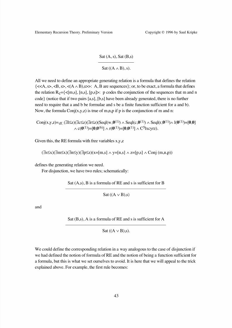
7/28/2019 Kripke Recursion Theory
http://slidepdf.com/reader/full/kripke-recursion-theory 47/191
Elementary Recursion Theory. Preliminary Version Copyright © 1996 by Saul Kripke
43
Sat (A, s), Sat (B,s)________________
Sat ((A ∧ B), s).
All we need to define an appropriate generating relation is a formula that defines the relation
{<<A, s>, <B, s>, <(A ∧B),s>>: A, B are sequences}; or, to be exact, a formula that defines
the relation Rc={<[m,s], [n,s], [p,s]>: p codes the conjunction of the sequences that m and n
code} (notice that if two pairs [a,s], [b,s] have been already generated, there is no further
need to require that a and b be formulae and s be a finite function sufficient for a and b).
Now, the formula Conj(x,y,z) is true of m,n,p if p is the conjunction of m and n:
Conj(x,y,z)=df. (∃l≤z)(∃c≤z)(∃r≤z)(Seql(w,0(1)) ∧ Seql(c,0(1)) ∧ Seql(r,0(1))∧ l(0(1))=[0,0]
∧ c(0(1))=[0,0(6)] ∧ r(0(1))=[0,0(1)] ∧ C5lxcyrz).
Given this, the RE formula with free variables x,y,z
(∃s≤x)(∃m≤x)(∃n≤y)(∃p≤z)(x=[m,s] ∧ y=[n,s] ∧ z=[p,s] ∧ Conj (m,n,p))
defines the generating relation we need.
For disjunction, we have two rules; schematically:
Sat (A,s), B is a formula of RE and s is sufficient for B_____________________________________________
Sat ((A ∨ B),s)
and
Sat (B,s), A is a formula of RE and s is sufficient for A_____________________________________________
Sat ((A ∨ B),s).
We could define the corresponding relation in a way analogous to the case of disjunction if
we had defined the notion of formula of RE and the notion of being a function sufficient for
a formula, but this is what we set ourselves to avoid. It is here that we will appeal to the trick
explained above. For example, the first rule becomes:
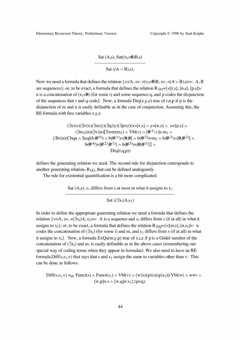
7/28/2019 Kripke Recursion Theory
http://slidepdf.com/reader/full/kripke-recursion-theory 48/191
Elementary Recursion Theory. Preliminary Version Copyright © 1996 by Saul Kripke
44
Sat (A,s), Sat((xi<0)B,s)
______________________
Sat ((A ∨ B),s).
Now we need a formula that defines the relation {<<A, s>, <(xi<0)B, s>, <(A ∨B),s>>: A, B
are sequences}; or, to be exact, a formula that defines the relation RD1={<[r,s], [n,s], [p,s]>:
n is a concatenation of (xi<0) (for some i) and some sequence q, and p codes the disjunction
of the sequences that r and q code}. Now, a formula Disj(x,y,z) true of r,n,p if p is the
disjunction of m and n is easily definable as in the case of conjunction. Assuming this, the
RE formula with free variables x,y,z
(∃s≤x)(∃r≤x)(∃n≤y)(∃q≤y)(∃p≤z)(x=[r,s] ∧ y=[n,s] ∧ z=[p,s] ∧
(∃m1≤n)(∃v≤n)[Term(m1) ∧ Vbl(v) ∧ [0(1),v]∈m1 ∧
(∃b≤n)(Cbqn ∧ Seql(b,0(5)) ∧ b(0(1))=[0,0] ∧ b(0(2))=m1 ∧ b(0(3))=[0,0(3)] ∧
b(0(4))=[0(2),0(1)] ∧ b(0(5))=[0,0(1)]] ∧
Disj(r,q,p))
defines the generating relation we need. The second rule for disjunction corresponds to
another generating relation, RD2, that can be defined analogously.
The rule for existential quantification is a bit more complicated:
Sat (A,s), s1 differs from s at most in what it assigns to xi_______________________________________________
Sat ((∃xi)A,s1)
In order to define the appropriate generating relation we need a formula that defines the
relation {<<A, s>, <(∃xi)A, s1>>: A is a sequence and s1 differs from s (if at all) in what it
assigns to xi}; or, to be exact, a formula that defines the relation REQ={<[m,s], [n,s1]>: n
codes the concatenation of (∃xi) (for some i) and m, and s1 differs from s (if at all) in what
it assigns to xi}. Now, a formula ExQu(m,y,p) true of x,i,z if p is a Gödel number of theconcatenation of (∃xi) and m, is easily definable as in the above cases (remembering our
special way of coding terms when they appear in formulae). We also need to have an RE
formula Diff(s,s1,v) that says that s and s1 assign the same to variables other than v. This
can be done as follows:
Diff(s,s1,v) =df. Funct(s) ∧ Funct(s1) ∧ Vbl(v) ∧ (w≤s)(p≤s)(q≤s1)((Vbl(w) ∧ w≠v ∧
[w,p]∈s ∧ [w,q]∈s1)⊃p=q).

7/28/2019 Kripke Recursion Theory
http://slidepdf.com/reader/full/kripke-recursion-theory 49/191
Elementary Recursion Theory. Preliminary Version Copyright © 1996 by Saul Kripke
45
Then REQ is definable by the following formula of RE with free variables x,y:
(∃s≤x)(∃s1≤y)(∃i≤y)(∃m≤y)(∃p≤y)(x=[m,s] ∧ ExQu(m,i,p) ∧ y=[p,s
1] ∧ Diff(s,s
1,i)).
Finally, we come to bounded universal quantification, which is a bit subtler than the
preceding cases. We have the rule
Sat ((xi<0(n))A,s), Sat (A,s1), s1 differs from s only in that s1 assigns n to xi, t denotes n+1
with respect to s, xi does not occur in t_____________________________________________________________________
Sat ((xi < t)A,s)
This says, roughly, that if s satisfies both (xi<0(n))A and A(0(n)), then s satisfies anyformula of the form (xi<t)A where t denotes n+1 with respect to s. The corresponding
relation is RUQ={<[m,s], [n,s1], [p,s]>: for some term t and some variable xi not occurring
in t, p codes the concatenation of (xi < t) and n, s1 differs from s at most in that it assigns a
number q to xi, and m is the concatenation of (xi<0(q)) and n}. Now, a formula
UnQu(m,i,t,p) which “says” that p is the Gödel number of (xi<t)A, where A is the formula
whose Gödel number is m, is easily definable as in the above cases (taking care of
remembering that we are not using the simple-minded coding scheme). Then we can define
RUQ by means of the following formula with free variables x,y,z:
(∃s≤x)(∃s1≤y)(∃m≤x)(∃n≤y)(∃p≤z)(∃i≤x)(∃t≤z)(∃q≤x)(∃r≤x)(Term(t) ∧ Vbl(i) ∧
(j≤t)(w≤t)([j,w]∈t⊃w≠i) ∧ UnQu(n,i,t,p) ∧ Diff (s,s1,i) ∧ Num(q,r) ∧ Den(i,r,s1) ∧
UnQu(n,i,q,m)∧ x=[m,s] ∧ y=[n,s1] ∧ z=[p,s]).
We are now done in our job of defining the generating relations corresponding to the
clauses in the inductive definition of satisfaction for RE. We now have to make sure that we
can define the relations that generate more and more complex formulae of the form (xi<t)A.
For conjunction, we have the rule
Sat ((xi<t)A, s), Sat ((xi<t)B,s), t denotes 0 with respect to s_________________________________________________
Sat ((xi<t)(A ∧ B), s).
The corresponding relation is RC*={<[m,s], [n,s], [p,s]>: for some q,r,xi,t such that xi is a
variable, t is a term, m codes the concatenation of (xi<t) and q, n codes the concatenation of
(xi<t) and r, the denotation of t with respect to s is 0 and p is the concatenation of (xi<t) and
the conjunction of q and r}. RC* is definable by the following formula with free variables
x,y,z:
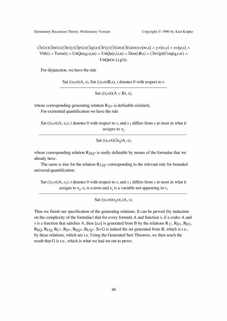
7/28/2019 Kripke Recursion Theory
http://slidepdf.com/reader/full/kripke-recursion-theory 50/191
Elementary Recursion Theory. Preliminary Version Copyright © 1996 by Saul Kripke
46
(∃s≤x)(∃m≤x)(∃n≤y)(∃p≤z)(∃q≤x)(∃r≤y)(∃i≤m)(∃t≤m)(x=[m,s] ∧ y=[n,s] ∧ z=[p,s] ∧
Vbl(i) ∧ Term(t) ∧UnQu(q,i,t,m) ∧ UnQu(r,i,t,n) ∧ Den(t,0,s) ∧ (∃w≤p)(Conj(q,r,w) ∧
UnQu(w,i,t,p))).
For disjunction, we have the rule
Sat ((xi<t)A, s), Sat ((xi<t)B,s), t denotes 0 with respect to s_________________________________________________
Sat ((xi<t)(A ∨ B), s),
whose corresponding generating relation RD* is definable similarly.
For existential quantification we have the rule
Sat ((xi<t)A, s1), t denotes 0 with respect to s, and s1 differs from s at most in what it
assigns to x j____________________________________________________________________
Sat ((xi<t)(∃x j)A, s),
whose corresponding relation REQ* is easily definable by means of the formulae that we
already have.
The same is true for the relation RUQ* corresponding to the relevant rule for bounded
universal quantification:
Sat ((xi<t)A, s1), t denotes 0 with respect to s, and s1 differs from s at most in what it
assigns to x j, t1 is a term and x j is a variable not appearing in t1____________________________________________________________________
Sat ((xi<t)(x j<t1)A, s).
Thus we finish our specification of the generating relations. It can be proved (by induction
on the complexity of the formulae) that for every formula A and function s, if a codes A and
s is a function that satisfies A, then [a,s] is generated from B by the relations RC, RD1, RD2,REQ, RUQ, RC*, RD*, REQ*, RUQ*. So G is indeed the set generated from B, which is r.e.,
by these relations, which are r.e. Using the Generated Sets Theorem, we then reach the
result that G is r.e., which is what we had set out to prove.
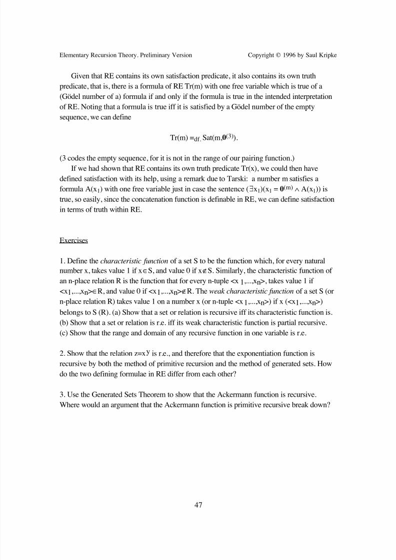
7/28/2019 Kripke Recursion Theory
http://slidepdf.com/reader/full/kripke-recursion-theory 51/191
Elementary Recursion Theory. Preliminary Version Copyright © 1996 by Saul Kripke
47
Given that RE contains its own satisfaction predicate, it also contains its own truth
predicate, that is, there is a formula of RE Tr(m) with one free variable which is true of a
(Gödel number of a) formula if and only if the formula is true in the intended interpretationof RE. Noting that a formula is true iff it is satisfied by a Gödel number of the empty
sequence, we can define
Tr(m) =df. Sat(m,0(3)).
(3 codes the empty sequence, for it is not in the range of our pairing function.)
If we had shown that RE contains its own truth predicate Tr(x), we could then have
defined satisfaction with its help, using a remark due to Tarski: a number m satisfies a
formula A(x1) with one free variable just in case the sentence (∃x1)(x1 = 0(m) ∧ A(x1)) is
true, so easily, since the concatenation function is definable in RE, we can define satisfaction
in terms of truth within RE.
Exercises
1. Define the characteristic function of a set S to be the function which, for every natural
number x, takes value 1 if x∈S, and value 0 if x∉S. Similarly, the characteristic function of
an n-place relation R is the function that for every n-tuple <x1,...,xn>, takes value 1 if
<x1,...,xn>∈R, and value 0 if <x1,...,xn>∉R. The weak characteristic function of a set S (orn-place relation R) takes value 1 on a number x (or n-tuple <x1,...,xn>) if x (<x1,...,xn>)
belongs to S (R). (a) Show that a set or relation is recursive iff its characteristic function is.
(b) Show that a set or relation is r.e. iff its weak characteristic function is partial recursive.
(c) Show that the range and domain of any recursive function in one variable is r.e.
2. Show that the relation z=xy is r.e., and therefore that the exponentiation function is
recursive by both the method of primitive recursion and the method of generated sets. How
do the two defining formulae in RE differ from each other?
3. Use the Generated Sets Theorem to show that the Ackermann function is recursive.
Where would an argument that the Ackermann function is primitive recursive break down?
7/28/2019 Kripke Recursion Theory
http://slidepdf.com/reader/full/kripke-recursion-theory 52/191
Elementary Recursion Theory. Preliminary Version Copyright © 1996 by Saul Kripke
48
4. Show that the set of Gödel numbers of formulae of the first order language of arithmetic
is r.e., using the Generated Sets Theorem. Do the problem explicitly as follows. Write the
basis clauses and generating clauses for the formulae themselves, and also show how theyare then translated into basis clauses and generating clauses for codes. Then indicate what
formula of RE results if we apply the argument in the proof of the Generated Sets Theorem
to this case. Do the same for the set of formulae obeying the nested quantifier restriction.
7/28/2019 Kripke Recursion Theory
http://slidepdf.com/reader/full/kripke-recursion-theory 53/191
Elementary Recursion Theory. Preliminary Version Copyright © 1996 by Saul Kripke
49
Lecture VII
The Enumeration Theorem. A Recursively Enumerable Set which is Not Recursive
Now that we have shown how to define satisfaction for RE within RE itself, we are ready to
prove what may be considered the fundamental theorem of recursion theory. First, let us
define a variant on the notion of satisfaction we defined above. If B is a formula whose
only free variable is x1, then we say the number n satisfies1 B just in case the unit sequence
<n> satisfies B. We may thus define
Sat1 (m, n) =df. (∃s) (Sat (m, s) ∧ (y∈s)(y=[[0(1),0(1)],n]) ∧ [[0(1),0(1)],n]∈s).
One could in general define Satk, satisfaction for formulae with k free variables, either
directly in a similar manner or by using the k-tupling function to reduce it to the case k=1.
We also use the notation W(e,n) for the relation that holds just in case Sat1(e,n) holds.
We now have the
Enumeration Theorem: There is a 2-place r.e. relation W such that for every r.e. set S,
there is an e such that S = {n: W(e,n)}.
Proof : Let We={x: W(e,x)}. Each set We is defined by Sat1 (0(e),x) and is therefore r.e. If,
on the other hand, S is an r.e. set, then it is defined by some RE formula B with one freevariable. We may assume that B's free variable is x1; letting e be a Gödel number of B, we
see that S = We.
The Enumeration Theorem is so called because W enumerates the r.e. sets. This theorem is
a standard theorem of recursion theory, though our presentation of it is not standard. When
recursion theory is presented in terms of Turing machines, for example, W(e, x) is usually
the relation e codes a Turing machine which gives output "yes" on input x for some fixed
method of coding up Turing machines, and is shown to be r.e. by constructing a Turing
machine which decodes the instructions given in e and applies them to the input x. In each
formalism for developing recursion theory, the relation W(e, x) will be a different relation.
(The notation ‘W’ originates in Kleene.)
In general, we can define a k+1-place relation Wk+1 which holds of a k+1-tuple
<e,n1,...,nk> if W(e, [n1,...,nk]) holds. This can be used to prove that Wk+1 enumerates the
k-place r.e. relations.
A very famous corollary of the Enumeration Theorem is the following:
7/28/2019 Kripke Recursion Theory
http://slidepdf.com/reader/full/kripke-recursion-theory 54/191
Elementary Recursion Theory. Preliminary Version Copyright © 1996 by Saul Kripke
50
Theorem. There is an r.e. set whose complement is not r.e. (thus, an r.e. set which is not
recursive).Proof : Let K be the set {x: W(x, x)}. K is clearly r.e., since it is defined by the formula
Sat1(x1, x1). However, -K is not r.e., and so K is not recursive. To see this, suppose -K
were r.e. Then we would have -K = We for some e. By the definition of K, we see that x∈
-K iff x ∉ Wx, so in particular e ∈ -K iff e ∉ We. But We = -K, so e ∈ -K iff e ∉ -K,
contradiction.
(This shows that negation is not definable in RE: if it were, the complement of any r.e. set
would be definable in RE, so in particular -K would be definable in RE.) This proof uses an
idea due to Cantor. As we will see, once we have this theorem, Gödel’s first incompleteness
theorem is just around the corner.
The fact (if it is one) about the intuitive notion of computability corresponding to the
enumeration theorem is that there is a semi-computable relation that enumerates all the semi-
computable sets. It follows from this that there is a semi-computable set that is not
computable. However, to prove the enumeration theorem for semi-computability, and thus
to prove that not all semi-computable sets are computable, it seems necessary to use
Church's Thesis. If there were a single language in which all computation procedures could
be written out, then the enumeration theorem would follow: simply find some way of
coding up this language numerically, and some effective way of decoding coded instructions
and applying them to arguments. However, if we do not assume Church's Thesis, then it isby no means obvious that there is such a language. At first glance it might appear that the
lesson of Gödel's work is that there is no single language in which all computation can be
represented, just as there is no single fully classical language in which everything can be
expressed. Every language will have some sort of Gödel-type limitation; it is a peculiarity
of the language RE that the limitation is not that it cannot express its own semantic notions
(as is the case with full first-order languages), but that it cannot express negation. But if it
turns out that there are some semi-computable sets and relations that are not expressible in
RE, then it is quite conceivable that all semi-computable sets and relations are computable
and that the enumeration theorem for semi-computability fails.
The fact that the enumeration theorem is so fundamental to recursion theory, and that its
proof for semi-computability requires Church's Thesis, indicates a limitation to how much
recursion theory can be developed for the informal notion of computability by starting with
intuitively true axioms about computability. Shoenfield tries this approach in his book on
recursion theory; he winds up assuming the enumeration theorem, and does not give a fully
convincing intuitive justification for it, since he in effect assumes that there is a single
language in which all computation procedures can be represented.
7/28/2019 Kripke Recursion Theory
http://slidepdf.com/reader/full/kripke-recursion-theory 55/191

7/28/2019 Kripke Recursion Theory
http://slidepdf.com/reader/full/kripke-recursion-theory 56/191
Elementary Recursion Theory. Preliminary Version Copyright © 1996 by Saul Kripke
52
matter whether '∈' means 'is a member of' or 'is satisfied by'. In fact, if you knew somehow
that the unrestricted comprehension scheme is inconsistent but didn't know why, you would
be able to see immediately that no first-order language can contain its own satisfactionpredicate. Consider the following interpretation of a first-order language with '∈' as its only
predicate: let the variables range over the formulae with one free variable of the language,
and assume that the language contains its own expressions in its own domain. Suppose that
we interpret '∈' by means of the 2-place relation S(y,x) which holds just in case y is a
formula with one free variable and x satisfies y. Then suppose that the language could
define its own satisfaction for formulae of one free variable. Then we would have a model
that would make the comprehension scheme true, because a formula A(x) can be taken to be
the object y, and then the principle says that x satisfies y if and only if A(x), which is of
course true. So any proof of the inconsistency of the comprehension principle proves that a
first order language cannot contain its own satisfaction predicate for formulae with one free
variable. Often, the results of Gödel and Tarski are presented as if they involved all kinds of
sophisticated ideas very different from these, but the inconsistency of the unrestricted
comprehension scheme is essentially what proves those results.
(Now, suppose that in the derivation of a paradox we used the unrestricted
comprehension axiom with n parameters. How are we going to interpret 'x ∈ y' in this case?
One way will be analogous to the reduction of satisfaction to truth that we saw for the case
of RE. We take y to range over the formulae with one free variable, or their codes, and 'x ∈
y' to be defined by "x satisfies y", where y will be, or code, the formula with one free
variable
(∃z1)...(∃zn)(z1=0(m1) ∧...∧ zn=0(mn) ∧ A(x, z1, ..., zn)),
where m1,...,mn are the parameters. We could also use a relation of substitution of terms for
free variables in formulae to specify how y will be, in a way indicated below. Or we could
define 'x ∈ y' with the help of the pairing function, as holding between a number and a pair
composed of (the code of) the formula A(x, z1, ..., zn) and a finite function assigning values
to all of the variables z1, ..., zn.)
We can use what we have learned about satisfaction to state some very general results
about the indefinability of truth. As long as the language L contains a name 'a' for each
object a in its domain, we can (in the metalanguage) define satisfaction for L in terms of
truth for L: an object a satisfies a formula A(x1) just in case the sentence A('a') is true
(where A('a') is got from A(x1) by replacing all free occurrences of x1 with 'a'). We can
turn this into a definition in L of satisfaction in terms of truth as long as L possesses certain
syntactic notions. Suppose, for example, L has function symbols Q and S denoting
functions q and s, where q(a) = 'a' for all a in L's domain, and s(A(x 1), t) = A(t) for all
formulae A(x1) and terms t. Then s(A(x1), q(a)) = A('a') for all A(x1) and a, and so the
formula Tr(S(y,Q(x))) of L will define satisfaction in L if Tr defines truth in L. Since
7/28/2019 Kripke Recursion Theory
http://slidepdf.com/reader/full/kripke-recursion-theory 57/191
Elementary Recursion Theory. Preliminary Version Copyright © 1996 by Saul Kripke
53
satisfaction for L is not definable in L, it follows that truth is not definable either. So in
general we see that, for fully classical L, the following conditions cannot jointly obtain:
1. Truth for L is definable in L.
2. The relation of substitution of terms for free variables is definable in L.
3. Every object in L's domain has a name, and moreover the function from an object to
its name is definable in L.
In fact, somewhat weaker conditions than 2 and 3 are also incompatible with 1. For
example, 3 may be replaced with: every object in L's domain is denoted by some term of L
and the relation t denotes x is definable in L. For suppose Den(t, x) defined that relation;
then the formula (∃z)(Den(z, x) ∧ Tr(S(y, z))) would define satisfaction in L in terms of
truth. (We could further weaken 3 by assuming only that every object a of L's domain has a
definite description D in L, and that we can specify D in terms of a within L.) Also, we can
use the trick remarked on by Tarski to avoid using the substitution function. An object a
will satisfy A(x1) just in case the sentence (∃x1)(x1 = 'a' ∧ A(x1)) is true (or (∃x1)(x1 = t ∧
A(x1)) is true for some term t denoting a, or (∃x1)(D(x1) ∧ A(x1) is true for some definite
description D of a), so as long as the function F(t, A(x1)) = (∃x1)(x1 = t ∧ A(x1)) is
definable in L, and 3 obtains, we can define satisfaction in terms of truth within L.
Moreover, F is itself easily definable in terms of concatenation (as long as terms for the
primitive symbols of L exist in L), and is anyway simpler than the substitution function,
which has to distinguish between free and bound occurrences of variables. To put it in asuccinct form, we see that a language cannot both define all the devices that can be used to
reduce truth to satisfaction and contain its own truth predicate.
So far, we have been concentrating on interpreted languages whose domains include all
the expressions of the language itself. However, we can generalize the discussion by
considering languages that can talk about their own expressions indirectly, via coding. Let
L be a language with a countable vocabulary and with an infinite domain D. Suppose we
had a function f mapping the elements of some subset D1 of D onto the formulae, or at least
onto the formulae with one free variable. Call this a coding function. Given any coding
function f for L, the relation {<y,x>: x is in D1 and f(y) is satisfied by x} of "coded
satisfaction" between elements of L's domain is not itself definable in L: if S(y,x) defined it,
then the unrestricted comprehension scheme, with 'x ∈ y' replaced by 'S(y,x)', would be true
in L, which we know to be impossible. Note that none of this depends on any particular
facts about f; any coding function will do, and we know that such a mapping will exist
whenever L has an infinite domain.
As before, this is related to the question of the definability of truth in L. Let us say that
a formula Tr(x) of L defines truth in L (relative to f) if Tr(x) defines {y: f(y) is true in L}.
We can always find a function f such that some formula of L defines truth in L relative to f
(for practically any L). For example, let L be the language of arithmetic, and let f "assign"
7/28/2019 Kripke Recursion Theory
http://slidepdf.com/reader/full/kripke-recursion-theory 58/191
Elementary Recursion Theory. Preliminary Version Copyright © 1996 by Saul Kripke
54
Gödel numbers to sentences of L so that the Gödel numbers of the true sentences of L are
0, 2, 4, ... and the Gödel numbers of false sentences of L are 1, 3, 5, ... (Or if arbitrary
formulae are to be coded rather than just sentences, we can let 0, 3, 6, ... code the truesentences, let 1, 4, 7, ... code the false sentences, and let 2, 5, 8, ... code the rest of the
formulae.) Relative to such a Gödel numbering, truth in L is obviously definable in L.
However, for any coding f, conditions 1-3 above will still not be jointly satisfiable, and so
for this particular Gödel numbering, the basic syntactic notions will not be definable in L.
For any ordinary Gödel numbering (e.g. our own numbering), the syntactic notions will be
definable, and so truth will be undefinable. But again, satisfaction will be undefinable for
any f, and for any L.
Now, as we have seen, if we drop the requirement that L be fully classical, these
indefinability results will no longer hold, since the language RE has its own satisfaction
predicate. However, RE does not have its own unsatisfaction predicate, i.e. there is no
formula U(y,x) of RE that obtains just in case x fails to satisfy y. (If there were, then we
could define -K in RE by U(x1, x1).) More generally, if L is a language with classical
semantics, but not necessarily with all classical connectives, then unsatisfaction is not
definable in L. To see this, suppose we had an unsatisfaction predicate U(y,x). Then letting
u be the formula U(y,y), we would have that U(u,y) obtains iff y does not satisfy U(y,y), and
so U(u, u) obtains iff u does not satisfy U(y,y); but to say that U(u, u) obtains is just to say
that u satisfies U(y, y), so this is impossible. Similarly, given suitable restrictions on L, a
language cannot have its own untruth predicate. Similar remarks apply when we allow
languages to talk about their formulae indirectly via codes.The enumeration theorem is really a form of the naive comprehension scheme for RE,
since the content of the theorem is that for every RE formula A(x1) there is an e such that
(x1)(A(x1) ≡ W(e, x1))
We cannot derive a contradiction by letting A be the formula ~W(x1, x1), since negation is
not definable in RE. This shows that it is essential to use either negation or unbounded
universal quantification in showing that scheme to be inconsistent for classical languages,
since RE lacks both negation and unbounded universal quantification. In fact, however,
there are languages which have unbounded universal quantification, as well as the other
logical symbols of RE, but which lack negation, and which have their own satisfaction
predicates; so only the use of negation is really essential.
From all of this it follows that, given our Gödel numbering, the language of arithmetic
does not have its own truth predicate. This was originally shown by Tarski as an
application of the work of Gödel. However, there it was presented in a more complicated
way as an application of the liar paradox. First, Gödel's self-reference theorem was used to
obtain, for any formula T(x1) of the language of arithmetic, a sentence A such that
7/28/2019 Kripke Recursion Theory
http://slidepdf.com/reader/full/kripke-recursion-theory 59/191
Elementary Recursion Theory. Preliminary Version Copyright © 1996 by Saul Kripke
55
A ≡ ~T(0(n))
is true, where n is the Gödel number of A. If T(x1) defined the set of truths of arithmetic,then we would also have
A ≡ T(0(n))
from which T(0(n)) ≡ ~T(0(n)) follows, which is self-contradictory. Intuitively, if T(x1)
means "x1 is true", then the sentence A says of itself that it is not true; so the Tarski-Gödel
proof can be seen as an application of the liar paradox. However, the construction of the
sentence A is rather tricky, and leaves one with the impression that something much more
subtle is going on here than actually is. In fact, when one takes the Tarski-Gödel proof
apart, one sees that it really boils down to the observation that arithmetic lacks its own
satisfaction predicate, which in turn is a direct consequence of the Russell paradox, as we
saw above.
Under the interpretation of '∈' as the relation of satisfaction, Russell's paradox is known
as 'the paradox of 'heterological''. Grelling was the discoverer of this paradox, and he
obtained it by reflecting on Russell's paradox. Call a predicate of English autological if it is
true of itself, and heterological otherwise. (For example, 'polysyllabic' is autological and
'monosyllabic' is heterological.) A problem arises when we ask whether 'heterological' is
itself heterological. 'heterological' is heterological iff 'heterological' is not true of
'heterological', iff 'heterological' is not heterological—a contradiction. If we interpret 'x∈ y'to mean 'y is true of x', then the formula 'x ∉ x' means that x is heterological, and the
derivation of the Grelling paradox is formally identical to the above derivation of the Russell
paradox.
Gödel mentions the liar paradox (and the paradox of Richard) as sources for the
reasoning leading to his theorems. He does not mention Russell's paradox, or the paradox
of 'heterological', although the Tarski-Gödel results are more naturally motivated by appeal
to them, as we have seen. That Russell's paradox and Grelling's paradox can be most
naturally put to this use is perhaps a fact known to some logicians, but to the author's
knowledge, it is not mentioned in the printed literature.
In fact, some logicians have probably misunderstood the relation between the liar
paradox on the one hand and Russell's and Grelling's paradoxes on the other. That the
Gödel-Tarski results can be motivated in the two ways is no surprise, for, in fact, on one
way of stating the liar paradox it just is the Grelling paradox. The liar paradox is
traditionally stated in terms of sentences like 'This sentence is false'. One way to get a liar
sentence without using locutions like 'this sentence' is via the sentence ''Yields a falsehood
when appended to its own quotation' yields a falsehood when appended to its own
quotation'. Since the result of appending the phrase mentioned in the sentence to its own
quotation is the sentence itself, the sentence says of itself that it is false. (A briefer way of
7/28/2019 Kripke Recursion Theory
http://slidepdf.com/reader/full/kripke-recursion-theory 60/191
7/28/2019 Kripke Recursion Theory
http://slidepdf.com/reader/full/kripke-recursion-theory 61/191
Elementary Recursion Theory. Preliminary Version Copyright © 1996 by Saul Kripke
57
Lecture VIII
Many-one and One-one Reducibility.
Given that not all sets are recursive, and indeed that some r.e. sets are not recursive, we may
want to ask of some nonrecursive set A whether the problem of deciding membership in it
can be reduced to that of deciding membership in some other set B. This idea gives rise to a
number of reducibility notions in recursion theory; in this section, we shall discuss two of
the simplest such notions.
We say that a set A is many-one reducible to B (in symbols, A ≤m B) if there is a total
recursive function φ such that for all m, m ∈ A iff φ(m)∈ B. (We also say m-reducible for
many-one reducible.) We also write φ: A ≤m B when φ is a total recursive function
satisfying this condition. If φ: A ≤m B and φ is 1-1, then we say that A is 1-1 reducible (or
1-reducible) to B (in symbols, A ≤1 B).
One way to think of this informally is in terms of oracles. Suppose there were an
oracle that could tell you, for an arbitrary number, whether it is an element of B. Then if A
≤m B, you will have a way to use the oracle to find out whether an arbitrary number is an
element of A: to see whether m∈A, simple compute φ(m) and consult the oracle. If the
oracle tells you that φ(m)∈ B, then you know that m ∈A, and if it tells you that φ(m)∉ B,
then you know that m ∉ A.
Here's a simple example of 1-1 reducibility. Let A be an arbitrary set, and let B = {2m:m∈A}. Then we see that A ≤1 B by letting φ(m) = 2m. And intuitively, we can effectively
determine whether m ∈A by consulting the oracle about whether 2m∈ B.
It can readily be shown that the relations ≤1 and ≤m are reflexive and transitive. Let us
write A ≡m B for A ≤m B & B ≤m A, and similarly for ≡1; it then follows that ≡m and ≡1 are
equivalence relations. The ≡m-equivalence classes are called many-one degrees or m-
degrees; similarly, the ≡1-equivalence classes are called 1-1 degrees or 1-degrees.
The relations ≤m and ≤1 do not coincide. To see this, let A = {even numbers}, and let
φ(m) = 0 if m is even, 1 if m is odd. Then we see that φ: A ≤m {0}. However, there is
clearly no 1-1 function φ such that x ∈ A iff φ(x)∈ {0}, so A is not 1-reducible to {0}.
A set is many-one complete r.e. (1-1 complete r.e.) iff it is r.e. and every r.e. set is
many-one reducible (1-1 reducible) to it. If S is many-one complete r.e., then every r.e. set
is of the form {x: φ(x)∈ S} for some total recursive φ. One example of a many-one
complete set (which is also 1-1 complete) is the set S = {[e, x]: x ∈ We}. To see that S is
1-1 complete, let S1 be any r.e. set. S1 is We for some e, so let φ(x) = [e, x]; x ∈ S1 iff x ∈
We iff φ(x)∈ S. φ is clearly as required; in particular, φ is recursive, since its graph is
defined by the formula y = [0(e), x]. Another 1-1 complete set is the set T of Gödel
numbers of true RE sentences. To see this, note that if A(x1) defines a set S1, then n ∈ S1
iff A(0(n)) is true; so if φ(n) is a recursive function that picks a Gödel number of A(0(n)) (for
7/28/2019 Kripke Recursion Theory
http://slidepdf.com/reader/full/kripke-recursion-theory 62/191
Elementary Recursion Theory. Preliminary Version Copyright © 1996 by Saul Kripke
58
example, the smallest one), then x ∈ S1 iff φ(x)∈ T. The set K can also be shown to be 1-1
complete, but the proof is a bit trickier.
If S1 ≤m S2 and S2 is r.e. (recursive), then S1 is also r.e. (recursive). An r.e. m-completeset cannot be recursive: if S were an m-complete recursive set, then K ≤m S, and this would
imply that K is recursive, which it is not.
Some questions about reducibility naturally arise. First, is there an r.e. set which is
neither recursive nor many-one complete? Emil Post answered this question in the
affirmative, and we shall prove his result later on in the course. Second, are there any many-
one complete sets that are not 1-1 complete? The answer is no; this result is surprising, and
the proof is nontrivial; we shall give the proof later on. (The notion of being 1-complete and
of being m-complete are also equivalent to the notion of being creative, which we shall
define later on.)
Despite Post's result, all (or practically all) naturally arising r.e. sets are either 1-1
complete or recursive. That is, while r.e. sets that are neither 1-1 complete nor recursive
exist in great abundance, they tend to arise as cooked-up counterexamples rather than sets
which are interesting for separate reasons. A common way to prove that an r.e. set is
nonrecursive is to show that some 1-1 complete set reduces to it, which implies that it is 1-1
complete.
Another way to put this is in terms of degrees. Among the r.e. 1-1 degrees (i.e. ≡1-
equivalence classes containing r.e. sets), there is a degree on top (the degree of 1-1 complete
sets), and, excluding the degrees containing finite and cofinite sets, a degree on the bottom
(the degree of recursive sets with infinite complements), and many degrees in between.However, all the naturally occurring r.e. sets are to be found on top or on the bottom.
Besides ≤m and ≤1, there are coarser-grained reducibility relations, all of which give an
intuitive notion of the idea that given an oracle for a set B, we can decide A. Post, who
originally formulated the notions of many-one and 1-1 reducibilities, gave a variety of
reducibility notions, still studied today. One of his notions, the broadest of all, was
supposed to capture the intuitive notion of being able to decide A given an oracle that will
answer all questions about set membership in B. He called this notion 'Turing-reducibility';
it has also been called 'relative recursiveness' and 'recursiveness in'. As we said above, Post
found an r.e. set that was not many-one complete (and therefore not 1-1 complete).
However, he was able to define another reducibility relation with respect to which this set
was still complete. In general, he found broader and broader reducibility relations, and more
complicated r.e. but not recursive sets that failed to be complete with respect to them.
However, he could not solve this problem for the basic notion of Turing-reducibility, and it
was a long-standing question whether there are any r.e. sets which are neither recursive nor
Turing-complete. This was answered in the affirmative in 1956 by Friedberg and Mucnik.
Two sets A and B are called recursively isomorphic (in symbols, A ≡ B) if there is a 1-1
total recursive function φ which maps N onto N, and such that B = {φ(x): x ∈ A}. (It
follows that φ-1 is also such a function and that A = {φ-1(x): x ∈ B}.) If A ≡ B, then it is
7/28/2019 Kripke Recursion Theory
http://slidepdf.com/reader/full/kripke-recursion-theory 63/191
Elementary Recursion Theory. Preliminary Version Copyright © 1996 by Saul Kripke
59
easy to see that A ≡1 B, since φ: A ≤1 B and φ-1: B ≤1 A. The converse is also true, and is
highly nontrivial. It was once proposed that recursion theory be regarded as the study of
those properties of sets of natural numbers which are invariant under recursiveisomorphism. In fact, nearly all the properties studied by recursion theory are of this
nature; however, there are some exceptions.
The Relation of Substitution
In several occasions we have mentioned the relation of substitution of a term for all the free
occurrences of a variable in a formula, noting that we could use it to give alternative proofs
of some results. For example, we could have given an alternative proof that RE defines its
own satisfaction using definitions of the notion of formula and of the relation of
substitution. Also, we could have defined truth in RE by means of satisfaction in RE using
substitution, instead of Tarski's trick. We will now show how a certain notion of “naive
substitution” is definable within RE, leaving as an exercise showing how to define the
notion of proper substitution.
First, we will define a relation that we will call “term substitution”: specifically, we
shall define the relation {<t1, t2, v, t>: the term t2 comes from the term t1 by replacing all
occurrences of the variable v, if any, by the term t; if v does not occur in t1, then t1=t2}. This
is defined by the following formula of RE:
TSubst(t1, t2, v, t) =df. Vbl(v) ∧ Term(t1) ∧ Term(t2) ∧ Term(t) ∧ [((j≤t1)~([j,v]∈t1) ∧ t1=t2)
∨ ((∃ j≤t1)([j+1,v]∈t1 ∧ (∃l≤t)(Seql(t,l+1)∧ Seql(t2,j+l+1) ∧ (y≤t)([l+1,y]∈t ⊃ [j+l,y]∈t2)
∧ (i≤ j+l)([i, [0(4), [0(1),0(1)]]]∈t2))))].
(Recall that all terms of RE are either of the form f 11...f 110 or of the form f 11...f 11xi, for some
i.)
We now show how to define the notion of “naive substitution”, that is the relation
{<m1, m2, v, m>: the sequence m2 comes from the sequence m1 by replacing all
occurrences of the variable v by the term m}. We call this “naive” substitution because the
result of a substitution of this kind may not be a formula, even if the expression operated
upon was one (note, for example, that even occurrences of the variable to be replaced within
quantifiers will be replaced, so if the replacing term is not a variable, substitution may
transform a quantifier into an expression that cannot form part of a formula.) Naive
substitution is definable by the following formula of RE:
NSubst(m1,m2,v,m)=df. (∃l≤m1)(Seql(m1,l) ∧ Seql(m2,l) ∧ (i≤l)(y≤l)[(([i,y]∈m1 ∧
~(∃ j≤y)([j,v]∈y))⊃ [i,y]∈m2) ∧ (([i,y]∈m1 ∧ (∃ j≤y)([j,v]∈y))⊃ (z≤m2)(TSubst(y,z,v,m)
⊃ [i,z]∈m2))]).
7/28/2019 Kripke Recursion Theory
http://slidepdf.com/reader/full/kripke-recursion-theory 64/191
7/28/2019 Kripke Recursion Theory
http://slidepdf.com/reader/full/kripke-recursion-theory 65/191
Elementary Recursion Theory. Preliminary Version Copyright © 1996 by Saul Kripke
61
________ ____
B (xi)A
A proof in L is a finite sequence of formulae of L such that each formula is either an axiom
or follows from earlier formulae by one of the inference rules. A sentence is a theorem just
in case it occurs in a proof. More generally, a proof from Γ , where Γ is a set of sentences of
L, is a finite sequence of formulae in which each formula is either an axiom or an element of
Γ , or follows from earlier formulae by the inference rules. A sentence is a theorem of Γ just
in case it occurs in a proof from Γ . We write fi A to mean that A is a theorem, and Γ fi A to
mean that A is a theorem of Γ .
Remarks. The axiom schemata 1-3, along with MP, are sufficient to prove all tautologies.
We could have simply taken all tautologies (of L) as axioms, but the present approach will
prove more convenient later.
The present system differs from standard systems in that axiom schemata 4 and 5 are
usually formulated as follows:
4'. (xi)A⊃A', where A' is got from A by replacing all free occurrences of xi in A by a
fixed term t, where either t is a constant, or t is a variable x j and no free occurrence
of xi in A falls within the scope of a quantifier (x j).
5'. A ⊃ (xi)A, where xi does not occur free in A.
All instances of 4' and 5' that are not also instances of 4 and 5 prove to be derivable and
hence redundant. As we said, 4 and 5 are simpler to represent in our coding of syntax than
4' and 5'.
(In any deductive system which contains a version of universal instantiation, some
restriction like that in 4 or 4' must be made, for the prima facie more natural scheme
(xi)A⊃ A', where A' comes from A by replacing all free occurrences of xi in A bya fixed term t
is invalid. To see this, consider the instance (x)(∃y) x ≠ y ⊃ (∃y) y ≠ y. In any
interpretation whose domain has more than one element and in which = is interpreted as
identity, this sentence is false. The problem is that the instantial term, y, becomes bound
once it is substituted for x; as long as we prevent this sort of thing, the restricted scheme will
be valid.)
We say that a system is sound just in case every theorem is valid, and every theorem of
Γ is a consequence of Γ , for any Γ . A system is complete if every valid sentence is a
theorem, and strongly complete if for all Γ , every consequence of Γ is a theorem of Γ . The
7/28/2019 Kripke Recursion Theory
http://slidepdf.com/reader/full/kripke-recursion-theory 66/191
Elementary Recursion Theory. Preliminary Version Copyright © 1996 by Saul Kripke
62
proof that our system is sound is fairly easy by induction on the length of a proof of any
given theorem. We will sketch later the argument for completeness (and strong
completeness), with more discussion of variant formulations, and in particular of thecomprehensive virtues and drawbacks of 4 and 5 as opposed to 4' and 5'. In particular, how
to derive 4' and 5' from 4 and 5 will be sketched later.
The Narrow and Broad Languages of Arithmetic.
By the narrow language of arithmetic, we mean the language as given in lecture I. Recall
that the primitive connectives of that language are ⊃ and ~ and that (xi) is the only primitive
quantifier; so, perversely, the logical vocabulary of the narrow language is disjoint from that
of RE. By the broad language of arithmetic we mean the language which has all the
vocabulary of the narrow language, and in addition the primitive connectives ∧ and∨ and the
quantifiers (∃xi), (xi < t), and (∃xi < t) (with the usual restrictions on t). So the broad
language of arithmetic literally contains the languages RE and Lim (but not Lim+). We
shall use L ambiguously to refer to both the broad and the narrow language of arithmetic;
when we wish to refer to them unambiguously, we shall use L- to refer to the narrow
language and L+ to refer to the broad language. Note that L- and L+ are equal in
expressive power, since the extra connectives of L+ are already definable in L-.
The language L+ has redundancies, as its extra connectives and quantifiers are already
definable in L-. L
-also has redundancies. For example, the negation sign is superfluous in
L-, as ~A is equivalent to A ⊃ 0 = 0'. If we had included the function symbols + and ., then
all the connectives would have been superfluous, since they could be eliminated in the
manner indicated in an exercise. Even in L+, we can eliminate all of the connectives except
for ∧. To see this, let A be any formula of L+, and let A* be an equivalent formula in which
A and M are replaced by + and .. Let A** be an equivalent formula in which no
connectives appear, constructed in the way indicated in lecture II. Finally, let A*** be a
formula of L+ got from A** by Russell's trick. Since the only connective that Russell's
trick introduces is ∧, ∧ is the only connective A*** contains; and A*** is equivalent to A.
Note that our deductive system only has axioms and rules for the connectives ~ and ⊃
and the quantifier (xi); when we are considering the broad language of arithmetic, we want
our system to prove all the valid formulae that contain the new logical vocabulary as well as
the old. This can be achieved by adding the following equivalence axiom schemes when we
are working in L+:
(A ∨ B) ≡ (~A ⊃ B)
(A ∧ B) ≡ ~(A ⊃ ~B)
(∃xi)A ≡ ~(xi)~A
(xi < t)A ≡ (xi)(Less(xi, t) ⊃ A)
7/28/2019 Kripke Recursion Theory
http://slidepdf.com/reader/full/kripke-recursion-theory 67/191
Elementary Recursion Theory. Preliminary Version Copyright © 1996 by Saul Kripke
63
(∃xi < t)A ≡ (∃xi)(Less(xi, t) ∧ A)
(Note that ≡ is a defined rather than a primitive symbol, even in L+.) It can be shown(though we will not show it here) that when these schemes are taken as axioms, every
formula of L+ is provably equivalent to a formula of L-, i.e. for every formula A of L+ there
is a formula A' of L- such that A ≡ A' is provable. Thus, the completeness of the system of
L+ follows from that for L-.
It is easy to show that the set of logical axioms for L (either L+ or L-) is r.e. We can
then prove, using the Generated Sets Theorem, that the set of provable formulae is r.e., and
that if Γ is an r.e. set of sentences of L, then the set of theorems of Γ is r.e. We can
generalize this to languages other than L. If K is a first order language such that the set of
formulae of K is r.e., then the set of provable formulae in K is r.e., and if Γ is an r.e. set of
sentences of K, then the set of theorems of Γ is r.e. For the set of formulae of K to be r.e.,
it is necessary and sufficient that the set {i: ai ∈ K} and the relations {<n, i>: Pni∈ K} and
{<n, i>: f ni∈ K} be r.e.
The Theories Q and PA.
There are two theories in the language L that are traditionally given special attention. One is
the theory Q, also called Robinson's Arithmetic (after its inventor Raphael Robinson). Q is
usually given in the language with + and., so our version of it is slightly nonstandard. In
the usual version, the axioms of Q are
1. (x1) 0 ≠ x1'
2. (x1)(x2) (x1' = x2' ⊃ x1 = x2)
3. (x1) (x1 = 0 ∨ (∃x2) x1 = x2')
4. (x1) x1 + 0 = x1
5. (x1)(x2) x1 + x2' = (x1 + x2)'
6. (x1) x1.0 = 0
7. (x1)(x2) x1.(x2') = x1
.x2 + x1
(Axioms 4-7 are usually called the recursion axioms.) To adapt this to our language, we
rewrite the axioms as follows:
1. (x1) 0 ≠ x1'
2. (x1)(x2) (x1' = x2' ⊃ x1 = x2)
3. (x1) (x1 = 0 ∨ (∃x2) x1 = x2')
4. (x1) A(x1, 0, x1)
5. (x1)(x2)(x3) (A(x1, x2, x3) ⊃ A(x1, x2', x3'))
7/28/2019 Kripke Recursion Theory
http://slidepdf.com/reader/full/kripke-recursion-theory 68/191
Elementary Recursion Theory. Preliminary Version Copyright © 1996 by Saul Kripke
64
6. (x1) M(x1, 0, 0)
7. (x1)(x2)(x3)(x4) ((M(x1, x2, x3) ∧ A(x3, x1, x4) ⊃ M(x1, x2', x4))
(Note that axioms 1-3 are unchanged.) In addition, we need existence and uniqueness
axioms for addition and multiplication:
(x1)(x2)(∃x3) (A(x1, x2, x3) ∧ (x4)(A(x1, x2, x4) ⊃ x4 = x3))
(x1)(x2)(∃x3) (M(x1, x2, x3) ∧ (x4)(M(x1, x2, x4) ⊃ x4 = x3))
(These are unnecessary for Q as it is usually stated, because their analogs in the language
with function symbols + and . rather than predicates A and M are logical truths.) Finally,
we did not include axioms for identity in our deductive system for the predicate calculus, so
we must include them here. The usual identity axioms are the reflexivity axiom (x1) x1=x1
and the axiom scheme (x1)(x2) (x1 = x2 ⊃ A ≡ A'), where A is any formula with at most x1
and x2 free and A' comes from A by replacing one or more free occurrences of x1 by x2. In
fact, we can get away with taking only finitely many instances of this scheme as axioms, and
the rest will be deducible. Specifically, we can take as our identity axioms the reflexivity
axiom and those instances of the above scheme in which A is an atomic formula not
containing the function symbol '. Since there are only finitely many predicates in L, there
are only finitely many such instances. Q, then, is the theory in L whose axioms are 1-7
above along with the existence and uniqueness clauses and the identity axioms just
specified.PA, or Peano Arithmetic, comes from Q by deleting axiom 3 and adding all those
sentences which are instances in L of the induction scheme:
[A(0) ∧ (x1)(A(x1) ⊃ A(x1'))] ⊃ (x1)A(x1).
(Axiom 3 is a theorem of the resulting system, so we need not take it as an axiom.)
The intuitive idea behind the induction scheme is that if zero has a property, and if
whenever a number n has that property n' does too, then every number has that property.
This was the intuition that Peano, and Dedekind before him, intended to capture, through an
induction axiom, that we could formalize
(P)([P(0) ∧ (x1)(P(x1) ⊃ P(x1'))] ⊃ (x1)P(x1)).
However, since in our languages we do not have quantification over arbitrary sets of natural
numbers, the induction axiom cannot be formalized in them. Unlike Dedekind's and Peano's
axiom, the induction scheme of the system we call 'Peano Arithmetic' only guarantees that
when zero has a property definable in L and when a number n has it n' does too, then every
number has it. So the induction scheme is really weaker than the intuitive idea behind it, that
7/28/2019 Kripke Recursion Theory
http://slidepdf.com/reader/full/kripke-recursion-theory 69/191
Elementary Recursion Theory. Preliminary Version Copyright © 1996 by Saul Kripke
65
Dedekind and Peano had in mind. In this respect, the name 'Peano Arithmetic' is somewhat
misleading.
The theory PA is adequate for elementary number theory, in the sense that all of elementary number theory can be carried out within PA. This is not obvious, however, and
requires proof. Notice, for example, that before the work of Gödel, it was not obvious that
such simple functions as exponentiation could even be defined in the language in which PA
is given, and exponentiation should certainly be regarded as a part of elementary number
theory. This illustrates another respect in which the name 'Peano Arithmetic' is misleading,
since it suggests that elementary arithmetic can be developed in that system in a
straightforward, obvious manner.
Exercises
1. Consider a language REexp which has the same terms, connectives and quantifiers as RE
but has only one predicate letter P31. P3
1xyz is interpreted as xy=z (it doesn't matter what to
say about the case 00; you can call P31xyz always false in that case, or give it the value 0 or
1). Prove that REexp defines the same sets and relations as RE. Prove also that in REexp
(for the same reason as in RE) disjunction is superfluous. (Remark: half of this exercise has
been done. To do the other direction, that is, defining the notions of RE in REexp, it is best
to proceed in the opposite order from what appears to be natural.)
2. Cantor proved that there can be no function φ mapping a set onto the set of all of its
subsets. Show directly that if there were such a mapping, then we would have an
interpretation of '∈' which makes true the unrestricted comprehension schema, including the
version with parameters. Remark: hence, any set-theoretical paradox that proves the
inconsistency of the schema also proves the theorem of Cantor in question. The case Cantor
actually used was once again the analog of Russell's paradox. Historically, this went the
other way around, since Russell discovered his paradox by analyzing Cantor's proof.
3. Show that the relations ≤m and ≤1 are reflexive and transitive.
4. Show that if A≤m B and B is r.e. (recursive), then A is r.e. (recursive).
5. For the language of arithmetic, prove using the Generated Sets Theorem that if a set of
axioms is r.e., then the set of theorems logically provable from it is r.e.
7/28/2019 Kripke Recursion Theory
http://slidepdf.com/reader/full/kripke-recursion-theory 70/191
Elementary Recursion Theory. Preliminary Version Copyright © 1996 by Saul Kripke
66
Lecture IX
Cantor's Diagonal Principle
A relation is called arithmetical if it is definable in L, the language of arithmetic. Since L
contains RE, it follows that all r.e. relations are arithmetical. Also, since L contains negation,
it follows that all complements of r.e. relations are arithmetical. That L contains negation
also implies that the enumeration theorem fails for arithmetical sets, i.e. there is no
arithmetical relation that enumerates all the arithmetical relations; similarly, there is no
recursive relation that enumerates all the recursive relations.
The best way to see this is by proving a general theorem. As in the enumeration
theorem for r.e. sets, if R is a two-place relation, we write Rx for {y: R(x, y)}. We give the
following
Definition: Let X be a set, F be a family of subsets of X, and R a two place relation
defined on X. R is said to supernumerate F iff for any S ∈ F, there is an x ∈ X such that
S = Rx. R is said to enumerate F iff R supernumerates F and for all x ∈ X, Rx ∈ F.
The content of the enumeration theorem is thus that there is an r.e. relation which
enumerates the r.e. sets. Next we have
Cantor's Diagonal Principle: The following two conditions are incompatible:
(i) R supernumerates F
(ii) The complement of the Diagonal Set is in F (the Diagonal Set is {x ∈ X: R(x, x)}).
Proof : Suppose (i)-(ii) hold. Then by (ii) X-{x ∈ X: R(x, x)} = {x ∈ X: ~R(x, x)} ∈ F.
By (i), {x ∈ X: ~R(x, x)} = Ry for some y. But then R(y, x) iff ~R(x, x) for all x ∈ X, so
in particular R(y, y) iff ~R(y, y), contradiction.
Cantor applied this lemma in the case F = power set of X to show that a set is never in1-1 correspondence with its own power set. We can apply it to formal languages by letting
F be the family of sets definable in a given language and letting R be a relation definable in
the language. Unless the language is very strange indeed, (ii) will be satisfied, so (i) will be
false. In the case of RE, we know from the enumeration theorem that (i) is satisfied, so it
follows that (ii) fails, and therefore that negation is not definable in RE. In the case of L, on
the other hand, (ii) holds, so (i) must fail. The same applies to the language Lim. Finally, if
we let F be the family of recursive sets and R be an arbitrary recursive relation, (ii) clearly
holds, so (i) fails and no recursive relation enumerates the recursive relations. (To see that
7/28/2019 Kripke Recursion Theory
http://slidepdf.com/reader/full/kripke-recursion-theory 71/191
Elementary Recursion Theory. Preliminary Version Copyright © 1996 by Saul Kripke
67
(ii) holds in this case, let R be a recursive relation, and let A(x, y) and B(x, y) define R and
-R, respectively, in RE. Then the diagonal set is defined in RE by A(x, x), and its
complement is defined by B(x, x).)
A First Version of Gödel's Theorem.
We now know enough to prove a version of Gödel's first incompleteness theorem. A
sentence is said to be undecidable in an axiom system Γ if neither it nor its negation is a
theorem of Γ , and Γ is said to be incomplete if some sentence is undecidable in it. We
normally use the same letter to denote a set of axioms and its set of theorems. If a set of
axioms is r.e., so is its set of theorems (by the Generated Sets Theorem). Similarly, if a set
of axioms is arithmetical, so is its set of theorems. We have the following
Theorem: Every arithmetical set Γ of true sentences of the language L is incomplete.
Proof : Since Γ consists of true sentences, if Γ were complete, then the true sentences of L
would be precisely the theorems of Γ . But as Γ is arithmetical, the set of theorems of Γ is
also arithmetical, i.e. definable in L. And as we have seen earlier, the set of true sentences of
L is not definable in L.
The theorem implies that every r.e. set of true sentences of L is incomplete.
In Gödel's original result the assumption that Γ is a set of true sentences was weakened,and hence Gödel's original result is stronger. An axiom system Γ in the language L is said
to be ω -consistent if there is no formula A(x) such that Γ fi (∃x)A(x) but Γ fi ~A(0(n)) for
all n. Obviously, an axiom system consisting of true sentences of L isω -consistent. An
axiom system can be consistent without being ω -inconsistent, however. Gödel showed (in
effect) that if Γ is an r.e. ω -consistent extension of Q, then Γ is incomplete. We shall not
prove the full result this time, though we shall prove some related results. Rosser later
showed that the assumption of ω -consistency can be weakened still further, and that no
consistent r.e. extension of Q is complete.
One of Gödel's main intents was to prove the theorem we just gave. The reason he gave
a stronger result must be understood in the light of the fact that, in the discovery andpresentation of his results, he was oriented by Hilbert's program. In a nutshell, Hilbert's
program demanded a proof of the consistency of the formal systems that codified the
theories of classical mathematics, a proof in which, roughly, no appeal to notions or
principles involving infinities was made: only so called 'finitistic' principles and methods of
proof were to be employed in proofs about the properties of formal systems. The notion of
truth in the standard interpretation of the language of arithmetic is a typically non-finitistic
one, and hence not usable within the context of Hilbert's program. However, the notions of
ω -consistency and consistency are finitistic.
7/28/2019 Kripke Recursion Theory
http://slidepdf.com/reader/full/kripke-recursion-theory 72/191
Elementary Recursion Theory. Preliminary Version Copyright © 1996 by Saul Kripke
68
More Versions of Gödel's Theorem
If B(xi) is a formula of L that defines a set S, let us say that a system Γ is correct for B if Γ
fi B(0(n)) implies that n ∈ S, and complete for B if n ∈ S implies that Γ fi B(0(n)).
Theorem: If Γ is r.e. and B defines a set which is not r.e., then Γ is not both correct and
complete for B. That is, the set S' = {n: Γ fi B(0(n))} is different from S.
Proof: This is simply because S' is r.e., since it is defined by the formula
(∃x)(∃m)(Num(m,n)∧NSubst(0(k),x,[0(1),0(i)],m) ∧ Th(x)) where Th(x) is an RE formula
defining the set of theorems of Γ and k is the Gödel number of B(xi) (we can use naive
substitution because we may assume that B does not contain bound occurrences of xi).
So when S is not recursively enumerable there's a difference between being an element of S
and being provably an element of S. If Γ is a true set of axioms, and thus correct, there will
be an instance B(0(n)) that is true but unprovable from Γ .
This is a slight generalization of a result due to Kleene. Kleene's result was that no r.e.
axiom system can be complete and correct for any formula that defines -K, and thus in
particular for the formula ~W(x, x). In fact, this holds for formulae defining -S whenever S
is a nonrecursive r.e. set.
Thus the interest of the theorem depends on the previous proof that there are r.e.nonrecursive sets (which in turn depends on the Enumeration Theorem). We can, however,
state a theorem which does not depend on this fact (or on any important fact of recursion
theory), and which says that any formal system must be incomplete for any formula
defining the complement of some r.e. set:
Theorem: If Γ is an r.e. set of true axioms, then there is an r.e. set S such that if A(x 1)
defines -S, some instance A(0(n)) is true but unprovable.
Proof: Suppose, for a contradiction, that for every r.e. set S at least one formula A(x1)
defining -S is such that Γ is complete for A. Then the following relation would be a
supernumeration of the complements of the r.e. sets: R(m,n)={<m,n>: m is a Gödel numberof a formula A(x1) and m is provable of n}; this relation is clearly r.e., using the same
reasoning as in the proof above. But now we can use Cantor's Diagonal Principle, and
conclude that the complement of the diagonal set {n:R(n,n)} cannot be the complement of
an r.e. set. But this is absurd, since {n:R(n,n)} is an r.e. set (if B(x,y) is an RE formula that
defines R, then B(x,x) defines {n:R(n,n)}).
Q is RE-Complete
7/28/2019 Kripke Recursion Theory
http://slidepdf.com/reader/full/kripke-recursion-theory 73/191
Elementary Recursion Theory. Preliminary Version Copyright © 1996 by Saul Kripke
69
Call a set Γ RE-complete if every true sentence of RE is a theorem of Γ , and RE-correct
if every theorem of Γ which is a sentence of RE is true. WheneverΓ fi A(0(n)) iff n ∈ S forall n, A(x) is said to weakly represent S in Γ , and S is said to be weakly representable in Γ
if some formula weakly represents it in Γ . (We also say that S is numerable in Γ .) Thus,
any r.e. set is weakly representable in any RE-complete and correct axiom system.
Moreover, if Γ is an r.e. set which is RE-complete and correct, then the sets weakly
representable in Γ are precisely the r.e. sets, since any set weakly representable in an r.e.
axiom system Γ is r.e. (To see this, recall that if A(xi) weakly represents S in Γ , k is a
Gödel number of A(xi), and Th(x) is an RE formula that defines the set of theorems of Γ ,
then the RE formula (∃x)(∃m)(Num(m,n) ∧NSubst(0(k),x,[0(1),0(i)],m) ∧ Th(x)) defines S.)
It turns out that Q is RE-complete and correct. Q is obviously RE-correct, because all
of its axioms are true; it takes a bit more work to show that Q is RE-complete. The main
fact we need to show this is
(Fact 1) Q fi (x1)(x1 < 0(n) ≡ (x1 = 0 ∨ ... ∨ x1 = 0(n-1))) for all n > 0, and
Q fi (x1) ~(x1 < 0)
Another useful fact is
(Fact 2) For all n, Q fi (x1)(x1 = 0(n) ∨ x1 < 0(n) ∨ 0(n) < x1)
Fact 2 is not necessary to prove that Q is RE-complete, however. We shall not prove either
fact, but we shall give a proof that Q is RE-complete.
It is also worth noting that a natural strengthening of Fact 2, namely that Q fi (x1)(x2)
(x1 = x2 ∨ x1 < x2 ∨ x2 < x1), is false. We can show this by constructing an interpretation
in which the axioms of Q are true but the statement (x1)(x2) (x1 = x2 ∨ x1 < x2 ∨ x2 < x1)
is false. The domain of this interpretation is N ∪ {α, β}, where α and β are two new
elements not in N. The constant 0 still denotes 0, and successor, addition and multiplication
have the same interpretations as before when restricted to the natural numbers. When the
arguments include α or β, we make the following stipulations:
Successor: α' = α, β' = β
Addition: n + α = α + n = α; n + β = β + n = β; α + α = α + β = α; β + β = β + α
= β
Multiplication: α.0 = β.0 = 0; α.n = α, β.n = β (n > 0); n.α = α, n.β = β (all n); α.α =
β.α = α; β.β = α.β = β
(where n ranges over the natural numbers) We leave it to the reader to verify that the
axioms of Q are true in this interpretation, but that neither α < β nor β < α holds.
7/28/2019 Kripke Recursion Theory
http://slidepdf.com/reader/full/kripke-recursion-theory 74/191
Elementary Recursion Theory. Preliminary Version Copyright © 1996 by Saul Kripke
70
We are now ready to prove our theorem about Q.
Theorem: Q is RE-complete.Proof : We show by induction on the complexity of sentences that every true sentence of
RE is a theorem of Q.
(1) Atomic sentences. First, note that every true atomic sentence involving = is
provable, since any such sentence is of the form 0(n) = 0(n) and therefore follows from the
identity axioms. Next, we show by induction on n that A(0(m), 0(n), 0(p)) is provable for all
m, where p = m + n. A(0(m), 0, 0(m)) follows from axiom 4 of Q and is therefore provable.
If Q fi A(0(m), 0(n), 0(p)), then by axiom 5 we see that Q fi A(0(m), 0(n+1), 0(p+1)). So Q
proves all the true atomic sentences involving A; that Q proves all the true atomic sentences
involving M follows similarly from the recursion axioms for multiplication.
(2) Conjunctions. Suppose A and B are theorems of Q if true. If their conjunction is
true, both of them are true, so both are provable, and so is their conjunction.
(3) Disjunctions. Similar to the preceding case.
(4) Existential quantification. Suppose any statement less complex than (∃x)A(x) is a
theorem of Q if true. If (∃x)A(x) is true, so must be one of its instances A(0(n)), which is
then provable. But then so is (∃x)A(x).
(5) Bounded universal quantification. Suppose (xi < 0(n))A is a true RE sentence.
Then all of A(0), ... A(0(n-1)) are true, and hence provable by the inductive hypothesis.
Therefore Q fi (xi)((xi = 0 ∨ ... ∨ xi = 0(n-1)) ⊃ A), and so by Fact 1, Q fi (xi)(xi < n ⊃ A).
It follows, as we have seen, that the sets representable in Q are precisely the r.e. ones.
We have a related result about Lim:
Theorem: Q proves, among the sentences of Lim, exactly the true ones.
Proof : This time, we show by induction on the complexity of sentences that for all
sentences A of Lim, Q fi A if A is true and Q fi ~A if A is false.
(1) Atomic sentences. We have already proved half our result; we only need to show
that all false atomic sentences are refutable in Q. Moreover, if we can show this for
sentences involving =, the result will follow for those involving A and M: if p ≠m + n, then
Q fi A(0(m), 0(n), 0(k)) (where k = m + n) and Q fi 0(k) ≠ 0(q), so by the uniqueness axiomfor A, Q fi ~A(0(m), 0(n), 0(p)); and similarly for multiplication.
First, observe that by axiom 1 of Q, Q fi 0 ≠ 0(n) when n > 0 (since then 0(n) is a term of
the form t'). Next, note that axiom 2 is equivalent to (x1)(x2) (x1 ≠ x2 ⊃ x1' ≠ x2'), so we
can show by induction on k that Q fi 0(n) ≠ 0(p) where p = n + k. It follows that whenever n
< m, Q fi 0(n) ≠ 0(m). Finally, by the identity axioms we have that Q fi 0(m)≠ 0(n).
(2) Negation. Suppose A is the sentence ~B. If A is true, then B is false and by the
inductive hypothesis Q fi ~B, i.e. Q fi A. If A is false, then B is true, so by the inductive
hypothesis Q fi B, so Q fi ~~B (= ~A).
7/28/2019 Kripke Recursion Theory
http://slidepdf.com/reader/full/kripke-recursion-theory 75/191
Elementary Recursion Theory. Preliminary Version Copyright © 1996 by Saul Kripke
71
(3) Conjunction and disjunction. These are straightforward, and we shall only do the
case of conjunction. Suppose A = (B ∧ C). If A is true, then so are B and C, so Q fi B, Q fi
C, and so Q fi (B ∧ C). If A is false, then either B or C is false; suppose B is. Then Q fi~B, so Q fi (~B ∨ ~C), and so Q fi ~(B ∧ C).
(4) Bounded universal and existential quantification. Again, we only do universal
quantification, as the other case is similar. If (xi < 0(n))A is true, then A(0), ..., A(0(n-1)) are
true, so Q fi A(0), ..., Q fi A(0(n-1)), and by Fact 1, Q fi (xi < 0(n))A. If (xi < 0(n))A is false,
then A(0(k)) is false for some k < n, so Q fi ~A(0(k)); Less(0(k), 0(n)) is a true sentence of
RE, so Q fi Less(0(k), 0(n)), and so Q fi (∃xi)(Less(xi, 0(n)) ∧ ~A) and Q fi ~(xi < 0(n))A.
A formula A(x) is said to binumerate a set S in a system Γ iff for all n, n ∈ S iff Γ fi
A(0(n)) and n ∉ S iff Γ fi ~A(n). If some formula binumerates S in Γ , then we say that S is
binumerable in Γ (or numeralwise expressible, or strongly representable, or even simply
representable). Clearly, if a set is binumerable in Γ then both it and its complement are
numerable, so in particular if Γ is r.e., then any set binumerable in Γ is recursive. So not all
r.e. sets are binumerable in Q. The converse, that all recursive sets are binumerable in Q, is
true but not evident at this point: if S is recursive, then we have some formula A which
numerates S in Q and some formula B which numerates -S, but we don't yet have a single
formula which numerates both S and -S. The theorem we just proved shows that all sets
definable in Lim are binumerable in Q, since if A(x) is a formula of Lim that defines S, then
A(x) binumerates S.
The facts about weak representability in Q just given also hold for arbitrary r.e.extensions of Q that have true axioms. However, they do not hold for arbitrary extensions
of Q, or even arbitrary r.e. extensions. For example, let Γ be an inconsistent set. Then Γ
clearly extends Q, but only one set is weakly representable in Γ , namely N itself (since for
any A and any n, A(0(n)) is a theorem of Γ ). Also, no set is strongly representable in Γ
(since we will always have Γ fi A(0(n)) and Γ fi ~A(0(n))). However, they do hold for
arbitrary consistent r.e. extensions of Q. That is, if Γ is a consistent r.e. extension of Q,
then the sets weakly representable in Γ are precisely the r.e. ones. (Again, it is easy to show
that all sets weakly representable in Γ are r.e.; the hard part is showing that all r.e. sets are
representable in Γ .) Moreover, as Shepherdson has shown, every r.e. set is weakly
represented in Γ by some formula that actually defines it, though it is not necessarily thecase that every formula that defines it weakly represents it in Γ . The proof of this result is
tricky, however. It is easier to prove if we only require Γ to be ω -consistent; we will prove
this later.
Let Γ be any consistent extension of Q whatsoever, and let A(x) be a formula of RE that
defines a set S. Then whenever Γ fi ~A(0(n)), n∉ S. To see this, suppose Γ fi ~A(0(n)) and
n ∈ S. Then A(0(n)) is a true sentence of RE, and so Q fi A(0(n)); since Γ extends Q, Γ fi
A(0(n)). But then both A(0(n)) and ~A(0(n)) are theorems of Γ , contradicting our
assumption that Γ is consistent. We thus have the following
7/28/2019 Kripke Recursion Theory
http://slidepdf.com/reader/full/kripke-recursion-theory 76/191
Elementary Recursion Theory. Preliminary Version Copyright © 1996 by Saul Kripke
72
Theorem: Any consistent extension of Q is correct for negations of formulae of RE.
7/28/2019 Kripke Recursion Theory
http://slidepdf.com/reader/full/kripke-recursion-theory 77/191
Elementary Recursion Theory. Preliminary Version Copyright © 1996 by Saul Kripke
73
Lecture X
True Theories are 1-1 Complete.
Theorem: If Γ is an r.e. set which is RE-complete and correct, then the theorems of Γ form
a 1-1 complete set.
Proof : Suppose Γ is such a set. Let S be any r.e. set, and let A(xi) be a formula of RE that
defines it; we can assume A to contain no bound occurrences of xi. We define φ(n) to be the
least among the Gödel numbers of A(0(n)). φ is recursive: its graph {<n,y>: φ(n)=y} is
defined in RE by the formula (∃m≤y)(Num(m,n) ∧NSubst(0(k),y,[0(1),0(i)],m) ∧ Th(x) ∧
(w<y)(~NSubst(0(k),w,[0(1),0(i)],m))) (where Th(x) is an RE formula defining the set of
theorems of Γ and k is the Gödel number of B(xi)); notice that the use of negation in the
last conjunct is legitimate, since the formula it affects is equivalent to a formula of Lim+.
Clearly φ is 1-1, and for any n, n ∈ S iff A(0(n)) is true, iff Γ fi A(0(n)), iff φ(n) belongs to
the set of Gödel numbers of theorems of Γ . So φ: S ≤1 {theorems of Γ }. Finally, the set of
theorems of Γ is r.e., and therefore is 1-1 complete.
It follows that the theorems of Q form a 1-1 complete set, and hence a nonrecursive set. In
fact, we can prove the stronger result that if Γ is any r.e. set of true axioms, the set of
theorems of Γ is 1-1 complete, as we will see shortly.
Let us say that a formula A(x) of the language of arithmetic nicely weakly represents aset S in a theory Γ if it weakly represents S in Γ and also defines S. We may similarly
define "nicely strongly represents". Similarly, a formula A(x1, ..., xn) nicely weakly
(strongly) represents an n-place relation R in Γ if it both weakly (strongly) represents R in
Γ and also defines R.
It follows from our results of the last lecture that any r.e. set is nicely weakly
representable in Γ whenever Γ is true and extends Q. We shall now see that the latter
requirement, that Γ extend Q, is unnecessary: any r.e. set is nicely weakly representable in
any set Γ of true axioms of the language of arithmetic. Before proving this, we shall need
the following theorem:
Deduction Theorem: For any set Γ and any sentences A and B (of any first-order
language), if Γ , A fi B then Γ fi A⊃ B. (Here, Γ , A fi B means Γ ∪ {A} fi B.)
Proof : Suppose Γ , A fi B, and let M be a model of Γ (i.e. an interpretation in which every
element of Γ is true). If A is true in M, then M is a model of Γ ∪ {A}, and so by the
soundness of the predicate calculus B is true in M, so A ⊃ B is true in M. If A is false in
M, then again A ⊃ B is true in M. So A⊃ B is true in all models of Γ , and therefore by the
completeness theorem Γ fi A⊃ B.
7/28/2019 Kripke Recursion Theory
http://slidepdf.com/reader/full/kripke-recursion-theory 78/191
Elementary Recursion Theory. Preliminary Version Copyright © 1996 by Saul Kripke
74
The proof we just gave is model-theoretic; however, it is possible to establish the
deduction theorem proof-theoretically, by showing how to transform any proof of B from Γ
∪ {A} into a proof of A ⊃ B from Γ . Such a proof-theoretic argument might be moresatisfying, since the model-theoretic argument merely shows that whenever a proof of A
from Γ ∪ {A} exists, then a proof of A ⊃ B from Γ exists, and leaves it an open question
whether there is any direct way to transform the former into the latter.
Now let A(x1) be any sentence of RE that defines a set S; we claim that the formula Q⊃
A(x1) nicely weakly represents S in any system Γ with true axioms. (By Q we mean here
some conjunction of the axioms of Q; such a conjunction exists because Q's axioms are
finite in number.) Clearly, Q⊃ A(x1) defines S; we must show that Q ⊃ A(0(n)) is a
theorem of Γ iff n ∈ S. First, suppose that n∈ S. Since Q is RE-complete, Q fi A(0(n)).
Clearly, Γ , Q fi A(0(n)). By the deduction theorem, Γ fi Q⊃A(0(n)). Conversely, suppose Γ
fi Q⊃ A(0(n)). Then since Γ is true, Q ⊃ A(0(n)) is also true. But Q is true, so A(0(n)) is
true. But A(0(n)) is a sentence of RE, and is true iff n ∈ S. So n ∈ S, and we are done.
Therefore we have established this
Theorem: If Γ is a set of true sentences of L, then every r.e. set is nicely weakly
representable in Γ .
Corollary: For such a Γ , the set of all theorems of Γ is a set to which all r.e. sets are 1-1
reducible. If Γ is r.e., then Γ 's theorems form a 1-1 complete set.
Note that, while every r.e. set is nicely weakly representable in such a Γ , we have not
shown that every r.e. set is nicely representable by every formula that defines it, or even
every RE formula that defines it. If we require Γ to extend Q, on the other hand, then every
RE formula that defines S represents it in Γ , because any such Γ is RE-complete and
correct.
Church's Theorem
Note that the empty set Ø is trivially a set of true axioms; it follows from our theorem thatevery r.e. set is nicely weakly representable in Ø, and therefore that Ø's theorems, i.e. the
valid formulae of L, form a 1-1 complete set (since Ø is r.e.). So the set of valid formulae
of L is not recursive (when the set of theorems of a theory is not recursive, the theory is
called undecidable; this use of the term 'undecidable' must not be confused with the use we
are familiar with, in which the term applies to sentences). This is called Church's Theorem.
Note that whether a formula is valid does not depend on the interpretation of the nonlogical
vocabulary, and therefore that Church's theorem does not depend on the interpretation of the
predicates and function symbols of L: for any language with two 3-place predicates, one 2-
7/28/2019 Kripke Recursion Theory
http://slidepdf.com/reader/full/kripke-recursion-theory 79/191
Elementary Recursion Theory. Preliminary Version Copyright © 1996 by Saul Kripke
75
place predicate, a constant, and a 1-place function symbol, the set of valid formulae of that
language is undecidable, and indeed 1-1 complete.
(Actually, there are two versions of Church's theorem, depending on whether the identitypredicate is regarded as a logical symbol. We have been regarding it as nonlogical; when it
is regarded as logical, so that the identity axioms are taken as logical axioms, Church's
Theorem states that the set of valid formulae (in the present sense of "valid") of a language
with two 3-place predicates, a constant and a 1-place function symbol is an undecidable set.
The proof is exactly the same.)
Clearly, this result also applies to first-order languages extending L. In fact, we can use
a few tricks to show that it also applies to some languages smaller than L. We already
know that the constant 0 is redundant in L, since the formula x = 0 is equivalent to (y)A(x, y,
x). We can also eliminate the successor function sign, since the graph of the successor
function is defined by (∃z)[(w)M(w, z, w) ∧A(x, z, y)]. Reasoning in this way, we can
show that Church's theorem applies to any language with two 3-place predicates. Using a
trick that we saw in an exercise, we can eliminate these predicates in favor of a single 3-place
predicate defining the graph of the exponentiation function plus a constant for 0 and a 1-
place function letter for successor. Using still more devious tricks, we can show that
Church's theorem applies to a language which contains only a single 2-place predicate.
However, we cannot go any further: the set of valid formulae of a language with only 1-
place predicates (with or without identity) is recursive.
(The reasoning we have given is not wholly rigorous. For one thing, while we can find a
language K which is properly included in L and which has the same expressive power, wemust also show that the above remarks about Q hold for some translation of Q into K. We
shall not enter into these considerations here; they will be addressed when we prove the
Tarski-Mostowski-Robinson theorem.)
The name "Church's Theorem", though traditional, does not make full justice to its
discoverers, since Turing proved the same theorem in his famous original paper on
computability; "the Church-Turing theorem" would be a more appropriate name. Also
Gödel, in his paper on the incompleteness theorems, stated a very closely related result
which, from our vantage point, establishes Church's theorem; but Gödel may not have
realized that this was a consequence of his result. Gödel's result is that for any formal
system with a primitive recursive set of axioms we can always find a sentence which is notquantificationally valid, but such that the statement that it is not quantificationally valid is not
provable in the system.
Complete Theories are Decidable
Theorem: Consider a language in which the set of all sentences is recursive, and let Γ be a
set of axioms in this language. If Γ is r.e. and the set of closed theorems of Γ is not
7/28/2019 Kripke Recursion Theory
http://slidepdf.com/reader/full/kripke-recursion-theory 80/191
Elementary Recursion Theory. Preliminary Version Copyright © 1996 by Saul Kripke
76
recursive (i.e., undecidable), Γ is incomplete.
Proof : We first give an informal proof using Church's Thesis. We can assume that Γ is
consistent, for otherwise the set of theorems of Γ is simply the set of all sentences, which byhypothesis is recursive. Suppose Γ is complete, and let A be any expression. We shall
show that either A or ~A is a theorem of Γ . Since the set of sentences of the language of Γ
is recursive, we can tell effectively whether A is a sentence. If A is a sentence, then since Γ
is complete, either A or ~A is a theorem of Γ . So to see whether A is a theorem of Γ or not,
simply run through all the proofs from Γ . If you encounter a proof of A, then A is a
theorem; if you encounter a proof of ~A, then A is not a theorem; and since Γ is complete,
you will eventually encounter a proof of A or of ~A, so this procedure will eventually
terminate. So we can effectively tell whether an arbitrary expression is a theorem of Γ , and
so the set of theorems of Γ is recursive.
We now reason more formally. Suppose Γ is complete; again, we may suppose that Γ
is consistent. Since Γ is r.e., the set of theorems of Γ is defined in RE by some formula
Th(x). Since Γ is complete, an expression A is a nontheorem of Γ just in case either A is a
nonsentence or ~A is a theorem. Thus the set of nontheorems of Γ is defined by an RE
formula N(x) ∨ (∃y)(Neg(x, y) ∧ Th(y)), where N(x) defines the set of nonsentences of the
language of Γ and Neg(x, y) defines the relation y is the negation of x. We know that such
an RE formula N(x) exists because by hypothesis the set of sentences of the language of Γ
is recursive, and Neg(x, y) is easily defined using concatenation. It follows that the set of
theorems of Γ is recursive.
It was a while before logicians realized this fact, despite the simplicity of its proof. This
may be because the decision procedure given is not intuitively a "direct" one, i.e. a
procedure which determines whether A is a theorem of Γ or not by examining A itself.
Note that the requirement that Γ be r.e. is essential here, as is seen by letting Γ equal the
set of true sentences of the language of arithmetic: the set of theorems of Γ , i.e. Γ itself, is
certainly not recursive, but it is complete, and the set of sentences of L is recursive.
Replacing Truth by ω -Consistency
Let us now state some incompleteness results aboutω -consistent, but not necessarily true
formal systems. School is the set of (consequences of) true atomic sentences of the
language of arithmetic and of true negations of atomic sentences.
Theorem: If Γ is arithmetical, ω -consistent and contains School, Γ is incomplete.
Proof: Suppose Γ was complete. Since Γ is arithmetical, it does not coincide with the set of
truths, so there must be a sentence A which is either true but unprovable or false but
provable from Γ . If A is false but provable, since the system is complete, ~A must be true
7/28/2019 Kripke Recursion Theory
http://slidepdf.com/reader/full/kripke-recursion-theory 81/191
Elementary Recursion Theory. Preliminary Version Copyright © 1996 by Saul Kripke
77
but unprovable (ω -consistency implies consistency), and so is any prenex version of it.
Take the shortest example B of a true but unprovable sentence: among the prenex true
unprovable sentences, take one with the shortest number of quantifiers. This sentence musthave some quantifiers, since if Γ contains School, all sentences made up from atomic
sentences by use of connectives are decidable in Γ . The first quantifier in B will not be
existential, because if it were, some instance of it would be true, and thus a shorter true but
unprovable statement (unprovable, because if it were provable so would be its existential
generalization). So the first quantifier in B must be universal, which means that all its
instances must be true and provable, since they are shorter. Since Γ is complete, ~B must
also be provable. But this contradicts the hypothesis that Γ is ω -consistent.
The theorem does not hold if we replace ω -consistency by consistency. There are consistent
arithmetical, even recursive, sets of sentences containing School (and extensions of School)
which are complete. An example is the set of truths in the structure of the real numbers with
a constant for 0 and function letters for successor, addition and multiplication. This is
naturally a complete set, which, by a celebrated result of Tarski, is recursive.
On the other hand, if Γ is r.e. and contains Q (not just School), the hypothesis of ω -
consistency in the theorem can be weakened to consistency. We will prove this later. Now
we can establish the following
Theorem: If Γ is r.e., ω -consistent and contains Q, then Γ is incomplete.
Proof: We know that if Γ contains Q, it is RE-complete and hence that it is correct fornegations of RE sentences. Let A(x1) be an RE-formula that defines K. Then ~A(x1)
defines -K. Since Γ is r.e., the set {n: ~A(0(n)) is a theorem of Γ } is r.e. and thus it does not
coincide with -K. Since Γ is correct for negations of RE sentences, there is no false provable
statement of the form ~A(0(n)), so there must be a statement of that form which is true but
unprovable. This does not yet tell us that A(0(n)) is also unprovable, since Γ need not be a
set of true sentences. Let's take again, from among the prenex true unprovable sentences of
the form ~A(0(n)), one with the shortest number of quantifiers. This sentence must have
some quantifiers, for the same reason as before. And it cannot begin with an existential,
again for the same reason. So the sentence must be of the form (x)C(x), and such that all of
its instances are provable. Now, A(0(n)) cannot be provable, since it is equivalent to ~(x)C(x)and that would contradict ω -consistency.
The Normal Form Theorem for RE.
Although our incompleteness results are quite powerful, it is a bit unsatisfying that we have
not been able to construct effectively examples of undecidable sentences. One way to do
this uses a result that we will prove now.
7/28/2019 Kripke Recursion Theory
http://slidepdf.com/reader/full/kripke-recursion-theory 82/191
7/28/2019 Kripke Recursion Theory
http://slidepdf.com/reader/full/kripke-recursion-theory 83/191
Elementary Recursion Theory. Preliminary Version Copyright © 1996 by Saul Kripke
79
enumeration theorem. From the normal form theorem, we see that the relation W(e, x) is
defined by some formula (∃y)T(e, x, y), where T is a formula of Lim without negation. T is
a particular formula, and therefore has a fixed number of bounded quantifiers and nounbounded quantifiers. It follows that there is a single fixed n such that every r.e. set is
defined by some formula with at most n bounded quantifiers and only one unbounded
quantifier. This leaves open the possibility that n must be very large; in fact, however, it is
known that n can be made rather small.
Whenever we have a normal form theorem, we can combine it with the enumeration
theorem to get an analogous result. The most spectacular enumeration theorem we have
mentioned is that proved by Matijasevic (building on earlier work by Davis, Putnam and
Julia Robinson), that every r.e. set or relation is definable by a formula of the form
(∃x1)...(∃xn) t1 = t2, where t1 and t2 are terms involving only the function symbols ', + and .
(and the constant 0 and the variables). Note that the formula t1 = t2 is simply a polynomial
equation. Thus the decision problem for any r.e. set is equivalent to the decision problem
for some polynomial equation with integer coefficients. The Matijasevic theorem alone
does not give us an indication of how large the degree of such equations can be, or of how
many variables they may contain. If we apply the enumeration theorem, however, we see
that the relation W(e, x) is defined by some particular formula (∃x1)...(∃xn) t1 = t2, whose
free variables are e and x. Let us indicate the free variable e by writing this formula as
(∃x1)...(∃xn) t1(e) = t2(e). Every r.e. set is therefore defined by the formula (∃x1)...(∃xn)
t1(0(e)) = t2(0(e)), for some particular e. So not only is the decision problem for every r.e.
set equivalent to the problem of solving some polynomial equation; we can alsosimultaneously bound the number of variables and the degree of the polynomial.
An immediate application of the normal form theorem is in the proof of the following
result:
Theorem: If Γ is r.e., ω -consistent and contains Q, then Γ is complete and correct for the
set of all formulae of the form (∃y)B, where B is a formula of Lim without negation.
Proof: Completeness: If (∃y)B is true, then B(0(n)) is true, for some n. So B(0(n)) will be
provable, since Q proves all the true sentences of Lim, and Γ contains Q. Therefore, (∃y)B
will be provable too. Correctness: Suppose (∃y)B is provable but false. Then all the
negations of its instances will be true: ~A(0), ~A(0')... So these are all provable, againbecause Q is complete for the true sentences of Lim. But this contradictsω -consistency.
Corollary: If Γ is r.e., ω -consistent and contains Q, then every r.e. set is nicely weakly
representable in Γ .
Corollary: If Γ is r.e., ω -consistent and contains Q, then the theorems of Γ form a 1-1
complete set.
7/28/2019 Kripke Recursion Theory
http://slidepdf.com/reader/full/kripke-recursion-theory 84/191
Elementary Recursion Theory. Preliminary Version Copyright © 1996 by Saul Kripke
80
The hypothesis of ω -consistency in these results could have been replaced by that of
consistency, but the corresponding proof is much trickier.
Exercises
1. Prove that if an r.e. set S1 is 1-1 complete, there is an infinite r.e. set S2 disjoint from S1.
2. Prove that a nonempty set is r.e. iff it is the range of a total recursive function.
Note: this result is the origin of the term 'recursively enumerable'. That is, a nonempty set S
is r.e. iff there is a recursive function φ that enumerates it, i.e. S={φ(0), φ(1),...}.
3. The Goldbach conjecture is the statement that every even integer greater than 2 is the sum
of two primes. Show that this conjecture can be written in the form (x)A, where A is in Lim.
Suppose that the conjecture, written in this form, is undecidable in the system we have called
Peano Arithmetic. What, if anything, would follow regarding the truth of the Goldbach
conjecture itself? (Explain your answer; if nothing follows, explain why, or if something
does follow, explain what follows and why.)
4. Proper substitution, as opposed to what we have called 'naive substitution', is the
substitution of a term for a variable, subject to the following restrictions. Only free
occurrences of the variable xi are to be replaced by the term t; and the substitution isimproper if any variable occurring in t becomes bound in the result. Define proper
substitution in RE, that is, PSubst(m1,m2,v,m). where m2 is the result of a proper
substitution of the term m for free occurrences of the variable v in m1. Use the following
fact: an occurrence of a variable xi within a term is bound in a formula iff the formula is a
concatenation of three sequences m, n and p, where the occurrence in question is in the part
corresponding to n, and n is (the Gödel number of) a formula beginning with (xi). m and/or
p are allowed to be empty. (This is a form of the usual definition.) Another treatment of
proper substitution, which is perhaps more elegant, will be sketched later. It should be clear
from the preceding why naive substitution is simpler, at least if this is the treatment adopted.

7/28/2019 Kripke Recursion Theory
http://slidepdf.com/reader/full/kripke-recursion-theory 85/191
7/28/2019 Kripke Recursion Theory
http://slidepdf.com/reader/full/kripke-recursion-theory 86/191
7/28/2019 Kripke Recursion Theory
http://slidepdf.com/reader/full/kripke-recursion-theory 87/191
Elementary Recursion Theory. Preliminary Version Copyright © 1996 by Saul Kripke
83
theorem. Let Γ be an r.e. system containing Q. Consider the relation Prov(x, y) which
holds if y is provable of x, i.e. if the result of replacing all (free) occurrences of x1 in the
formula (coded by) y by the numeral for x is provable. We can take Prov to be Σ1, since itcan be written out in RE; so it is of the form (∃z)L(x, y, z) for some formula L(x, y, z) of
Lim. Consider the formula ~Prov(x1, x1); it has some Gödel number m. Let G be the
sentence ~Prov(0(m), 0(m)), i.e. ~(∃z)L(0(m), 0(m), z). Suppose G is provable; that is,
suppose the formula ~Prov(x1, x1) is provable of m. Then L(0(m), 0(m), 0(k)) holds for
some k; since this is a true sentence of Lim, it is provable, and so (∃z)L(0(m), 0(m), z) is
provable. But G, which we are supposing to be provable, is just the sentence ~(∃z)L(0(m),
0(m), z). So if our system is consistent, G is not provable after all, i.e. ~Prov(x1, x1) is not
provable of m. But what G says is that the formula with Gödel number m, namely
~Prov(x1, x1), is not provable of m; so G is true. Therefore G is true but unprovable. As
long as the system is Σ1-correct, its negation is not provable either, and as we have seen, it
suffices for this that the system be ω -consistent.
Presented in this way, the proof seems rather tricky, and the undecidable sentence is
produced in a very devious way. As we have previously presented it, Gödel's theorem
should seem more like the inevitable outcome of the Russell paradox. In fact, there is a way
of viewing Gödel's original proof which makes it look this way.
Recall the proof that any fully classical language lacks its own satisfaction predicate. If
L, for example, has a predicate Sat(y,x) which defines the relation {<x, y>: y codes a
formula which x satisfies}, then L has a predicate Het(x) = ~Sat(x, x), which defines the set
of (Gödel numbers of) heterological formulae. But then if we ask whether Het(x) is itself heterological, we can derive a contradiction. (Indeed, that there is no formula defining the
set of heterological formulae follows directly from the inconsistency of the instance
(∃y)(x)(x ∈ y ≡ x ∉ x) of the unrestricted comprehension scheme, as we saw before.) It
follows from the indefinability of satisfaction that the formula Prov does not define
satisfaction.
We can show directly that the Gödel sentence G is true but unprovable, in a way that
imitates the reasoning of the last paragraph. Call a formula Gödel heterological if is not
provable of itself; the formula ~Prov(x1, x1) defines the set of Gödel heterological formulae.
Let us write this formula as GHet(x1). Now we ask, is "Gödel heterological" Gödel
heterological? The statement that "Gödel heterological" is Gödel heterological is simply thestatement GHet(0(m)), where m is the Gödel number of GHet(x1). Rather than leading to a
contradiction, our question has a definite answer "yes". Suppose "Gödel heterological"
were not Gödel heterological, i.e. that GHet(x1) were provable of m. If GHet(x1) is
provable of m, then Prov(0(m), 0(m)) is a theorem of Q and therefore of any system
extending Q; note that GHet(0(m)) is simply the negation of Prov(0(m), 0(m)). So if
GHet(x1) is provable of itself, then our system is inconsistent, since both Prov(0(m), 0(m))
and its negation are provable; so if our system is consistent, then GHet(x1) is not provable
of itself, i.e. is Gödel heterological. This is simply to say that GHet(0(m)) is true but not

7/28/2019 Kripke Recursion Theory
http://slidepdf.com/reader/full/kripke-recursion-theory 88/191
7/28/2019 Kripke Recursion Theory
http://slidepdf.com/reader/full/kripke-recursion-theory 89/191
Elementary Recursion Theory. Preliminary Version Copyright © 1996 by Saul Kripke
85
is recursive if R is; the same applies to the class of relations definable in Lim and to the
arithmetical relations. And this argument can easily be generalized to relations of more than
two places.A trickier case is the class of r.e. relations. The above argument will not show that this
class has the uniformization property, since y = µzR(x, z) will not in general be r.e. when R
is. To see this, let X be any r.e. set which is not recursive, and let R be the r.e. relation {<x,
y>: (y = 0 ∧ x ∈ X) ∨ y = 1}. Let S be the relation y = µzR(x, z). If x ∈ X, then S(x) = 0,
but if x ∉ X, then S(x) = 1. So if S is r.e., then -X can be defined in RE by S(x, 0'). But by
hypothesis X is nonrecursive, so S is not r.e.
However, we can use a somewhat trickier proof to show that uniformization holds for
the r.e. relations. Let R be any 2-place r.e. relation, and let F(x, y) be some formula of RE
that defines it. By the normal form theorem, we can take F to be (∃z)L(x, y, z) for some
formula L of Lim. (∃z)L(x, y, z) is equivalent to (∃w)(y = K1(w) ∧ L(x, K1(w), K2(w))).
We can now define a uniformizing relation S by (∃w)(y = K1(w) ∧ L(x, K1(w), K2(w)) ∧ (u
< w)~L(x, K1(u), K2(u))) (intuitively, w is the smallest code of a pair [y,z] for which L(x,y,z)
holds). Since L is a formula of Lim, the formula defining the uniformizing relation is a Σ1
formula and so S is an r.e. relation. This can be generalized to n+1-place r.e. relations in a
fairly obvious way. So we have proved the
Uniformization Theorem for r.e. Relations: The class of r.e. relations has the
uniformization property.
Corollary: Every r.e. relation can be uniformized by a partial recursive function with the
same domain.
The Normal Form Theorem for Partial Recursive Functions.
An application of the proof of the uniformization theorem for r.e. relations is a normal form
theorem for partial recursive functions, due to Kleene. Let φ be any partial recursive
function, and let R be its graph. R is defined by some Σ1 formula (∃z)L(x, y, z). As in the
proof of the uniformization theorem, we see that R is defined by y = K1(µwL(x, K1(w),K2(w))). Since L(x, K1(w), K2(w)) is a formula of Lim, and K1 is a function whose graph
is definable in Lim, we have the following:
Normal Form Theorem for Partial Recursive Functions: Every n-place partial
recursive function is of the form U(µwR(x1, ..., xn, w)) for some relation R definable in Lim
and some function U whose graph is definable in Lim.
Proof : The case n = 1 was just proved, and the general case is proved similarly.
7/28/2019 Kripke Recursion Theory
http://slidepdf.com/reader/full/kripke-recursion-theory 90/191
Elementary Recursion Theory. Preliminary Version Copyright © 1996 by Saul Kripke
86
This is not exactly what Kleene originally proved; he only required R and U to be primitive
recursive.
It is important not to forget the U; it is not true that every partial recursive function is of the form µwR(x1, ..., xn, w) for some R definable in Lim. Even if we allow R to be an
arbitrary recursive relation, this is still wrong. If, on the other hand, we require the function
φ to be total, then φ(x1, ..., xn) is µy(φ(x1, ..., xn) = y), so we can drop the U by taking R to
be φ's graph; but then we cannot require R to be definable in Lim.
7/28/2019 Kripke Recursion Theory
http://slidepdf.com/reader/full/kripke-recursion-theory 91/191
7/28/2019 Kripke Recursion Theory
http://slidepdf.com/reader/full/kripke-recursion-theory 92/191
7/28/2019 Kripke Recursion Theory
http://slidepdf.com/reader/full/kripke-recursion-theory 93/191
7/28/2019 Kripke Recursion Theory
http://slidepdf.com/reader/full/kripke-recursion-theory 94/191
7/28/2019 Kripke Recursion Theory
http://slidepdf.com/reader/full/kripke-recursion-theory 95/191
Elementary Recursion Theory. Preliminary Version Copyright © 1996 by Saul Kripke
91
characteristic function, and let R(x, y) be some formula which represents φ in Q, and
therefore in Γ . (Such an R exists by the preceding theorem.) Let B(x) be the formula R(x,
0'). If n ∈ S, then φ(n) = 1, so Γ fi R(0(n), 0'). If, on the other hand, n∉ S, then φ(n) = 0,so Γ fi (y)(R(0(n), y) ⊃ y = 0), so Γ fi ~R(0(n), 0') (since 0≠0' is a theorem of Q). So R(x,
0') strongly represents S in Γ .
This corollary extends our previous result: before, we only knew that every set definable in
Lim is strongly representable in Q (and therefore in any consistent extension of Q).
We can use our results to prove Rosser's form of Gödel's theorem:
Rosser's Theorem: If Γ is a consistent r.e. extension of Q, then Γ is incomplete.
Proof: We can give two different proofs using results we have proved. The first, closer in
spirit to Rosser's is this. Consider the function Φ(x, x). We know that the sets S1={m:
Φ(m, m) = 0}, and S2={m: Φ(m, m) is defined and > 0} are recursively inseparable. Let
A(x, y) be a formula that represents the function Φ(x, x) in Γ . So we have that if Φ(m, m) =
0 then Γ fi A(0(m), 0) ∧ (y)(A(0(m), y)⊃ y = 0); and if Φ(m, m) is defined and =n> 0 then
Γ fi A(0(m), 0(n)) ∧ (y)(A(0(m), y)⊃ y = 0(n)). By the second conjunct in the last formula,
if Φ(m, m) is defined and > 0, Γ fi ~A(0(m), 0). Since Γ is consistent, it is not the case that Γ
fi A(0(m), 0) and Γ fi ~A(0(m), 0). Let R1={m: Γ fi A(0(m), 0)} and R2={m: Γ fi ~A(0(m),
0)}. These are disjoint (since Γ is consistent) and, if Γ were complete, they would be the
complement of each other (and so exhaust N). They are r.e., for the usual reasons. So if
they were the complement of each other, they would be recursive, and then R1 would be arecursive set that would separate S1 and S2, and we prove that no set does that. So we can
conclude that Γ is not complete.
A second way of proving the theorem is the following. Suppose, for a contradiction, that
Γ is a consistent r.e. extension of Q that is complete. Since Γ is complete, the set of
theorems of Γ is recursive. Consider the relation R = {<e, m>: e is a Gödel number of a
formula A(x1), and A(0(m)) is a theorem of Γ }. Γ being recursive, R is a recursive relation.
Moreover, R enumerates the recursive sets, in the sense that each recursive set is Re for
some e. To see this, let S be a recursive set, and let A(x1) be a formula that strongly
represents it in Γ ; then if e is a Gödel number of A(x1), S = {m: Γ fi A(0(m))} = Re. So R
is a recursive enumeration of the recursive sets. But as we saw in Lecture IX, this isimpossible. Therefore, no such Γ can exist, and so any r.e. consistent Γ extending Q is
incomplete.
Exercises
1. (a) Prove that an infinite set S of natural numbers is r.e. iff it is the range of a 1-1 total
recursive function.

7/28/2019 Kripke Recursion Theory
http://slidepdf.com/reader/full/kripke-recursion-theory 96/191
Elementary Recursion Theory. Preliminary Version Copyright © 1996 by Saul Kripke
92
(b) Prove that an infinite set S of natural numbers is recursive iff it is the range of a 1-1
monotone increasing total recursive function.
(c) Prove that every infinite r.e. set has an infinite recursive subset.
2. Reduction property within Q. (a) If S1 and S2 are two r.e. sets, prove that there are two
r.e. sets S1' and S2' such that S1'⊆S1, S2'⊆S2, and S1'∪S2'=S1∪S2, such that S1' is
weakly represented by a formula A(x) and S2' by a formula B(x) and (x)~(A(x)∧B(x)) is a
theorem of Q.
(b) Hence, if two r.e. sets S1 and S2 are in fact disjoint, they can be weakly represented
by two formulae A(x) and B(x) such that (x)~(A(x)∧B(x)) is a theorem of Q.
3. (a) Show that the following instance of the naive comprehension scheme is
inconsistent: (∃y)(x)(x ∈ y ≡ ~(∃w)(x ∈ w ∧ w ∈ x)).
(b) Analogous to the construction of K using Russell's paradox, use the result in (a) to
obtain a corresponding r.e. set which is not recursive.
(c) Given an r.e. axiom system Γ extending Q, define a number n to be Gödel-
unreciprocated if m is a Gödel number of a formula A(x1) and there is no n such that n is
the Gödel number of a formula B(x1) with A(0(n)) and B(0(m)) both provable in Γ .
(Otherwise, m is Gödel-reciprocated .) Show, analogously to the treatment of 'Gödel-
heterological', that the sentence '"Gödel-unreciprocated" is Gödel-unreciprocated' has the
properties of the Gödel statement, i.e. it is a Π1 statement that is true but unprovable if Γ is
consistent and not disprovable if Γ is ω -consistent. (Note: this is the Gödelian analog of the paradox of part (a), and is meant to illustrate the theme that set-theoretic paradoxes can
be turned into proofs of Gödel's theorem.)
4. (a) Show that there is a recursive function ψ (m,n) such that ψ (m,n) is a code of the n-
term sequence all of whose terms are m.
(b) The Upwards Generated Sets Theorem says that if G is a set generated by a
recursive basis set and some recursive generating relations such that for each generating
relation R, the conclusion of R is greater than or equal to all of the premises, then G is
recursive. Prove this theorem. [Hint: prove that every element m of G occurs in a proof sequence for G such that all elements preceding m in the sequence are strictly less than m.
Then use (a).]
(c) Use (b) to prove that the set of Gödel numbers of formulae of the narrow first order
language of arithmetic is recursive.
(d) Extend this result to any first order language (in the narrow formulation) with
finitely many function letters and primitive predicate letters and constants.
5. Gödel's Theorem via a language with self-reference and extra constants.
7/28/2019 Kripke Recursion Theory
http://slidepdf.com/reader/full/kripke-recursion-theory 97/191
Elementary Recursion Theory. Preliminary Version Copyright © 1996 by Saul Kripke
93
The following is a method of proving the Gödel theorem that directly captures the idea that
the Gödel sentence says "I am not provable". It goes by adding additional constants to the
narrow first order language of arithmetic; as we have formulated that language, it has only asingle constant a1 standing for zero. We now add all of the others (a2, a3, ...) which will
denote various numbers. Call the expanded language L*. If we have a set Γ of axioms in L,
once we know what we want the extra constants to denote, Γ * will be obtained by adding to
Γ all axioms of the form an+1 = 0(mn), where mn is the number we want an+1 to denote.
(We may not care what certain of the an+1's denote, in which case we do not add any axiom
involving an+1 to Γ *.) Notice that the language L* and the axiom system Γ * are a mere
variant of L and Γ , since all we've done is to add special names for various particular
numbers, and nothing can be expressed or proved that couldn't be expressed or proved
already.
(a) Use the last remark to prove that if Γ is expanded to an axiom set Γ * with at most
one axiom of the given form for each constant, then any proof in Γ * can be transformed
into a proof in Γ by replacing each constant by the corresponding numeral and using the
axiom (x)(x=x).
(b) Hence, show that every theorem of Γ * becomes a theorem of Γ when constants in
the theorem, if any, are replaced by the corresponding numerals. Also show that Γ * is
consistent iff Γ is, and that the same holds for ω -consistency.
Now let us make a particular choice of mn, as follows: if n is a Gödel number of a
formula A of L in which x1 does not occur bound (but in which variables other than x1 may
occur free), let mn be the least Gödel number of the formula A(an+1) obtained from A bynaive substitution of x1 by an+1 throughout, and include the sentence an+1 = 0(mn) in Γ *.
(Notice that intuitively, if A says something A(x1), then under our interpretation of the
meaning of an+1, A(an+1) says "I have property A(x1)". Observe that what numbers are the
Gödel numbers of a given formula is independent of which interpretation we give to the
extra symbols.)
(c) Show that if Γ r.e., then so is Γ * and therefore so is the set of theorems of Γ *.
(d) Show that there is therefore aΠ1 formula (x2)B(x1, x2), where B(x1, x2) is a
formula of Lim, and which is satisfied by precisely those numbers that are not Gödel
numbers of theorems of Γ . We may assume that in this formula x1 does not occur bound.
Let n be the smallest Gödel number of this formula. Assume that Γ extends Q. Prove thatif Γ is consistent, then (x2)B(an+1, x2) is true but not provable from Γ *, and therefore that
(x2)B(0(mn), x2) is also true but unprovable from Γ .
(e) Show that if Γ * is ω -consistent, then ~(x2)B(an+1, x2) is not provable from Γ * and
that if Γ is ω -consistent, ~(x2)B(0(mn), x2) is not provable from Γ .
Remark: (d) and (e) prove Gödel's theorem both for Γ * and for the original system Γ . The
point of this exercise is to show that the use of "self-reference" in Gödelian arguments,
usually obtained by a rather indirect method, can be obtained by directly constructing a
7/28/2019 Kripke Recursion Theory
http://slidepdf.com/reader/full/kripke-recursion-theory 98/191
7/28/2019 Kripke Recursion Theory
http://slidepdf.com/reader/full/kripke-recursion-theory 99/191

7/28/2019 Kripke Recursion Theory
http://slidepdf.com/reader/full/kripke-recursion-theory 100/191
Elementary Recursion Theory. Preliminary Version Copyright © 1996 by Saul Kripke
96
The Smn Theorem.
If R is a 2-place r.e. relation, then intuitively Rk should be r.e. as well; but furthermore,given k, we ought to be able to effectively find an index for R k. This is indeed the case, and
is a special case of the Smn theorem. More generally, let R be an m+n-place r.e. relation. In
the case we have just considered, Rk is obtained from R by fixing k as a parameter; the
general form of the Smn theorem (put informally) says that given m numbers k1, ..., km, we
can effectively find an index for the relation obtained from R by fixing k1, ..., km as
parameters. In our own formalism, the Smn theorem is an easy consequence of the
definability in RE of substitution. We now state the S11 theorem, i.e. the special case of the
Smn theorem in which m = n = 1.
Theorem: For any 2-place r.e. relation R, there is a 1-1 recursive function ψ such that, for
all k, Wψ (k)= Rk.
Proof : Let e be an index for R. e is a Gödel number of some formula of RE A(x2,x1) that
defines R. An index of Rk, i.e. a Gödel number of a formula of RE that defines Rk, can be
obtained from e via substitution. More specifically, we define the graph of ψ in RE by the
formula PS(k,y)=df. (∃p≤y)(Num(p,k)∧ (w<p)~Num(w,k)∧ NSubst(0(e),y,[0(1),0(2)],p) ∧(w<y)(~NSubst(0(e),w,[0(1),0(2)],p))) (the use of negation is legitimate, since the formulae it
affects are equivalent to formulae of Lim). Informally, ψ assigns to k the least Gödel
number of the formula obtained by substituting the least Gödel number of the numeral of k
for x2 in the formula with Gödel number e. The function thus defined is clearly 1-1, sincethe results of substituting different numerals for the same variable in the same formula must
have different Gödel numbers.
The general form of the Smn theorem can be stated and proved similarly: for any m+n-place
r.e. relation R, there is a 1-1 recursive function ψ such that, for all k1,...,km,
Wn+1ψ (k1,...,km)= Rk1,...,km (where Rk1,...,km is {<y1, ..., yn>: R(k1, ..., km, y1, ..., yn)}). As
we see, the name "Smn theorem" derives from the convention of taking m as the number of
parameters and n as the number of other variables; 'S' probably stood for 'substitution' in the
original conception of Kleene, to whom the theorem is due.
As a consequence of the above theorem, we have the following
Theorem: For all m and n, there is a one to one m+1-place recursive function ψ such that
for all m+n-place r.e. relations R, if e is an index of R and k1, ..., kn are numbers, then ψ (e,
k1, ..., km) is an index of {<y1, ..., yn>: R(k1, ..., km, y1, ..., yn)}.
Proof : Apply the previous form of the Smn theorem to the relation Wm+n+1. That is, let ψ be
a function such that ψ (e, k1, ..., km) is an index of {<y1, ..., yn>: W(e, k1, ..., km, y1, ..., yn)}
= {<y1, ..., yn>: R(k1, ..., km, y1, ..., yn)}.

7/28/2019 Kripke Recursion Theory
http://slidepdf.com/reader/full/kripke-recursion-theory 101/191
7/28/2019 Kripke Recursion Theory
http://slidepdf.com/reader/full/kripke-recursion-theory 102/191
7/28/2019 Kripke Recursion Theory
http://slidepdf.com/reader/full/kripke-recursion-theory 103/191
7/28/2019 Kripke Recursion Theory
http://slidepdf.com/reader/full/kripke-recursion-theory 104/191
Elementary Recursion Theory. Preliminary Version Copyright © 1996 by Saul Kripke
100
incorporated into the system itself. We can already see from Gödel's first incompleteness
theorem that Hilbert's aim was unattainable. For if consistency was provable, then the
statement that every Π1 provable statement is true would be provable. But if this wasprovable, the Gödel sentence G, which is Π1, would be such that 'G is provable ⊃ G' would
be a theorem; but G says of itself that it is not provable, so '~G ⊃ G' would be a theorem,
and so by logic G would be a theorem. And this would imply, by the first incompleteness
theorem, that the system was not consistent after all.
Let us now give our proof of Gödel's second incompleteness theorem. First, let us see
how to write out the first incompleteness theorem in the language of arithmetic. Pick aΠ1
formula A(x) which defines -K, and fix a recursive function ψ as in the uniform effective
form of Gödel's theorem proved above. Then
For all e, if We is consistent and We extends Q, then A(0(ψ (e))) is true but unprovable,
from which it follows that
(†) For all e, if We is consistent and We extends Q, then A(0(ψ (e))) is true.
(We leave out the second part on the hypothesis of ω -consistency.) We shall write out (†)
in the language of arithmetic. We have in effect already seen how to write out the statement
that We is consistent. We have an RE formula Th(e, x) which says that x is a theorem of
We; We is consistent just in case 0 ≠ 0 is not a theorem of We, so We is consistent iff esatisfies ~Th(e, 0(n)), where n is a Gödel number of 0 ≠ 0; let us write Con(e) for ~Th(e,
0(n)). (Alternatively, we could let Con(e) be the sentence (∃x)~Th(e, x), since We is
consistent iff at least one sentence is not provable from We; or we could let Con(e) be the
statement that no sentence and its negation are both provable from We.) And we can easily
write "We extends Q" within the system: Q has finitely many axioms A1, ..., Ak, so let n1,
..., nk be their Gödel numbers; We extends Q just in case e satisfies Th(e, 0(n1)) ∧ ... ∧Th(e, 0(nk)). Let us write "e ext. Q" for this formula. Finally, let PS(x, y) be some formula
that weakly represents ψ in Q. Now consider the statement
(*) (e)(Con(e) ∧ e ext. Q ⊃ (∃y)(PS(e, y) ∧ A(y)))
(*) is a partial statement of the first incompleteness theorem, and therefore ought to be
provable in reasonably strong systems of number theory. Now consider the theory Q+(*).
Gödel's Second Incompleteness Theorem: If We is a consistent extension of Q+(*),
then Con(0(e)) is not a theorem of We, i.e. We does not prove its own consistency.
Proof: Suppose We extends Q* and Con(0(e)) is one of its theorems. Then as (*) is a
theorem of We, Con(0(e)) ∧ 0(e) ext. Q ⊃ (∃y)(PS(0(e), y) ∧ A(y)) is also a theorem of
7/28/2019 Kripke Recursion Theory
http://slidepdf.com/reader/full/kripke-recursion-theory 105/191
Elementary Recursion Theory. Preliminary Version Copyright © 1996 by Saul Kripke
101
We; we already know that Con(0(e)) is a theorem of We, and 0(e) ext. Q is a true sentence
of RE and is therefore a theorem of Q and therefore of We; so (∃y)(PS(0(e), y) ∧ A(y)) is a
theorem of We. Let f = ψ (e). Since PS represents ψ in Q, We fi PS(0(e), 0(f)) ∧(y)(PS(0(e), y) ⊃ y = 0(f)); it follows that A(0(f)) is a theorem of We. But we already
know from the first incompleteness theorem that A(0(f)) is unprovable in We if We is a
consistent extension of Q. Since We is an extension of Q, it follows that We is
inconsistent.
The theorem does not show that there are no statements which might be thought of as
expressing the consistency of a system which are not provable in the system, pathological
statements of consistency, so to speak. To see this, let Γ be an arbitrary consistent r.e.
extension of Q, let Pr'(x) be Pr(x) ∧ x ≠ 0(n) (where Pr(x) is any Σ1 formula defining the
set of theorems of Γ , and n is the Gödel number of 0 ≠ 0), and let Con'Γ be the sentence
~Pr'(0(n)). Since Γ is consistent, 0 ≠ 0 is not a theorem of Γ , so Pr'(x) defines the set of
theorems provable in Γ ; if Γ is ω -consistent, then Pr'(x) weakly represents the theorems of Γ in Γ as well. So in a sense, Con'Γ says that Γ is consistent. However, it is clear that Γ fi~Pr(0(n)), i.e. Γ fi Con'Γ . Also, we know from the exercises that if we have two disjoint r.e.
sets, we have weak representations of them which are provably disjoint in Q. If we take the
two sets to be on the one hand the set of theorems of Γ , and on the other hand the set of
sentences whose negation is a theorem of Γ , we therefore have weak representations of them
which are provably disjoint in Q. We might think that the corresponding sentence expresses
consistency. One of the aims of Feferman's, and of Jeroslow's, work, was to give conditionsfor distinguishing these pathological statements from statements for which Gödel's second
incompleteness theorem goes through.
An important point about our presentation of Gödel's second incompleteness theorem,
where it differs from other presentations, including Feferman's, is that in the hypothesis of
the theorem we only require that a single statement (namely, the conjunction of Q and (*))
be a theorem of a system for it to fail to prove its consistency. In other presentations of the
theorem, including Gödel's original presentation, the proof that a system does not prove its
own consistency requires assuming that a certain sentence, different for each system, is a
theorem of the system. Let G be a Gödel sentence for a system Γ which extends Q and let
ConΓ be a sentence in the language of arithmetic that says that Γ is consistent. The firstincompleteness theorem states that if Γ is consistent, then G is true but unprovable, so in
particular, if Γ is consistent, then G is true. So if Γ is a powerful enough system to prove
the first incompleteness theorem, then Γ fi ConΓ ⊃ G. If Γ fi ConΓ , then Γ fi G; since G is
true but unprovable from Γ , it follows that ConΓ is not a theorem of Γ . This is how the
second incompleteness theorem was originally proved, as a corollary of the first
incompleteness theorem. Thus, the unprovability of consistency for different Γ 's under this
presentation is proved under the hypothesis that different sentences are provable in these
different Γ 's — if Γ and ∆ are different systems, then to conclude that neither Γ nor ∆ prove
7/28/2019 Kripke Recursion Theory
http://slidepdf.com/reader/full/kripke-recursion-theory 106/191
Elementary Recursion Theory. Preliminary Version Copyright © 1996 by Saul Kripke
102
their consistency one must assume that Γ fi ConΓ ⊃ G, and that ∆ fi Con∆ ⊃ D (where D is
a Gödel sentence for ∆).
On our approach, taking ConΓ to be Con(0(e)), where e is an index for Γ , we give asingle sentence (*) such that any consistent r.e. Γ which extends Q + (*) fails to prove
ConΓ . Without any job of formalization at all, it is shown that any extension of Q+(*)
satisfies the second incompleteness theorem. And a system that does not contain Q+(*) is
not sufficient for elementary number theory, since it should be clear that the methods used
in class can be regarded as methods of elementary number theory.
This much we can say without any formalization at all. And we can presume that some
systems are strong enough to contain elementary number theory, and therefore to prove
Q+(*). So we know enough at this point to state the main philosophical moral of the
second incompleteness theorem -a system in standard formalization strong enough to
contain elementary number theory cannot prove its own consistency. Strictly speaking we
have stated this only for formalisms whose language is the first-order language of
arithmetic, but the technique is easily extended to first-order systems in standard
formalization with a richer vocabulary. Some ideas as to how to consider such systems will
become clear when we discuss the Tarski-Mostowski-Robinson theorem in a later lecture.
If one wishes to consider a specific system, such as the system we have called 'PA', we
can say in advance that it satisfies the conditional statement that if it contains elementary
number theory, it cannot prove its own consistency in the sense of Con(0(e)) above.
However, we have a task of formalization if we wish to show that the system contains
elementary number theory or at any rate Q+(*). Here is one of the misleading features of the name 'Peano arithmetic' that has been used for this system: it gives the impression that
by definition the system contains elementary number theory, when in fact it requires a
detailed formalization to show that this is so. If, for example, the properties of
exponentiation or factorial could not be developed in it, it would not contain elementary
number theory after all. We have seen the basic idea of how to do this, but the formalization
here is not trivial. Thus it does require a considerable task of formalization to show that (*)
can be proved in PA, and hence that the appropriate statement Con(0(e)) is not provable in
PA. But it requires no formalization at all to claim that any system in standard formalization
containing elementary number theory fails to prove its own consistency.
7/28/2019 Kripke Recursion Theory
http://slidepdf.com/reader/full/kripke-recursion-theory 107/191
7/28/2019 Kripke Recursion Theory
http://slidepdf.com/reader/full/kripke-recursion-theory 108/191
Elementary Recursion Theory. Preliminary Version Copyright © 1996 by Saul Kripke
104
arithmetic, we know that the predicate Tr(x) saying that x is the Gödel number of a true
sentence cannot be defined in arithmetic itself. We know also that the opposite situation
holds for the language RE. Either way, we have the following corollary which, like thelemma itself, holds for both the language of arithmetic and the language RE:
Corollary: Let A(x) be any formula in one free variable in the language of arithmetic (or
RE). Then there is a sentence G of the language of arithmetic (or of RE) with Gödel
number n such that G≡A(0(n)) and A(0(n))≡Tr(0(n)) are both true.
There are numerous ways of proving the self-reference lemma. Given our Gödel
numbering, G cannot actually be the sentence A(0(n)), since the Gödel number of A(0(n))
must be larger than n. However, it is possible to devise a different Gödel numbering such
that for every formula A(x), there is a number n such that A(0(n)) gets Gödel number n.
(This method of proving the self-reference lemma was discovered independently by
Raymond Smullyan and the author.) If we add extra constants to our language, then we can
prove a version of the self-reference lemma for the expanded language. Specifically, let L*
be the language obtained from the language of arithmetic by adding the constants a2, a3, ...
(a1 is already in L). Interpret the new constants as follows: if n is a Gödel number of a
formula A(x1), then interpret an+1 as the least Gödel number of A(an+1). Then the sentence
A(an+1) says of itself that it is A. Note that if mn is the Gödel number of A(an+1), the
sentence an+1 = 0(mn) is true under this interpretation. If we let Q* be the axiom system
obtained from Q by adding as axioms all sentences of the form an+1 = 0(mn)
, then Q* fiA(an+1) ≡ A(0(mn)) for all n, so we can let G be the sentence A(an+1). So if we chose to
work in the language L* rather than L, we could get the self-reference lemma very quickly;
moreover, L* does not really have greater expressive power than L, since L* simply assigns
new names to some things that already have names in L. Using this version of the self-
reference lemma it is also possible to prove Gödel's incompleteness theorem, as we have
seen in an exercise.
The proof of the self-reference lemma essentially due to Gödel employs the usual Gödel
numbering and constructs the sentence G in a more complicated way. Let A(x) be given.
Let φ be a recursive function such that if y is the Gödel number of a formula C(x1), then
φ(n, y) is the Gödel number of C(0(n)). Let B(x, y, z) represent φ in Q, and let A'(x, y) bethe formula (∃z)(B(x, y, z) ∧ A(z)). If y is the Gödel number of a formula C(x1), then A'(n,
y) holds iff the Gödel number of C(0(n)) satisfies A(x). (We can read A'(x, y) as "y is A of
x"; for example, if A(x) is "x is provable", then A'(x, y) is "y is provable of x".) Let m be
the Gödel number of A'(x1, x1), and let G be the sentence A'(0(m), 0(m)). (A(x1, x1) says
that x1 is A of itself, and G says that "is A of itself" is A of itself.) We shall show that Q fi
G ≡ A(0(n)), where n is the Gödel number of G. Note that G is really (∃z)(B(0(m), 0(m), z)
∧ A(z)), where B represents φ in Q. Note also that φ(m, m) is the Gödel number of G itself,
since m is the Gödel number of A'(x1, x1) and G is A'(0(m), 0(m)); so Q fi B(0(m), 0(m),

7/28/2019 Kripke Recursion Theory
http://slidepdf.com/reader/full/kripke-recursion-theory 109/191
7/28/2019 Kripke Recursion Theory
http://slidepdf.com/reader/full/kripke-recursion-theory 110/191
Elementary Recursion Theory. Preliminary Version Copyright © 1996 by Saul Kripke
106
A(0(n), y1, ..., ym)), where n is a Gödel number of G.
The version of the self-reference lemma in which G does not have free variables is simplythe special case of this lemma in which n = 0. Naturally, there is an effective version of the
self-reference lemma with free variables.
A corollary of the self-reference lemma with free variables is the following:
Corollary: Let A(x, y) be a formula of the language of arithmetic (or RE) with all free
variables shown; then there is a formula G(y) of the language of arithmetic (or of RE) with
Gödel number n such that (y)(G(y) ≡ A(0(n),y)) and (y)(A(0(n),y) ≡ Sat(0(n),y)) are both
true.
(In the case of RE, Sat(x,y) is W(x,y). In the case of the language of arithmetic, Sat(x,y),
which we use to mean that y satisfies the formula of the language of arithmetic with Gödel
number x, is not itself a formula of the language.)
The self-reference lemma with free variables might be given the name "self-reference
lemma with parameters", but this name is more appropriate for the following variant of the
lemma.
Self-Reference Lemma With Parameters: For any formula A(x), there is a recursive
function ψ and a formula PS(x, y) that representsψ in Q, such that for all m, ψ (m) is the
Gödel number of the formula (∃z)(PS(0(m)
, z) ∧ A(z)), and furthermore this formula isprovably equivalent in Q to A(0(ψ (m))).
Proof : Let χ be a recursive function such that if m is the Gödel number of a formula B(x1,
x2), then χ(m, n, p) is the Gödel number of the formula B(0(n), 0(p)). Let CH(x, y, z, w) be
a formula that represents χ in Q. Let n be the Gödel number of the formula (∃x3)(CH(x1,
x1, x2, x3) ∧ A(x3)), and let PS(x, y) be the formula CH(0(n), 0(n), x, y). PS represents the
function ψ (x) = χ(n, n, x); to prove the theorem, we only have to show that ψ (m) is the
Gödel number of the formula (∃z)(PS(0(m), z) ∧ A(z)), for any m. Since n is the Gödel
number of (∃x3)(CH(x1, x1, x2, x3) ∧ A(x3)), it follows that ψ (m) = χ(n, n, m) = the Gödel
number of (∃x3)(CH(0(n), 0(n), 0(m), x3) ∧ A(x3)), which is the formula (∃x3)(PS(0(m),
x3) ∧ A(x3)).Now, notice that (∃z)(PS(0(m), z) ∧ A(z)) is provably equivalent to A(0(ψ (m))). Thus,
writing G(x) for (∃z)(PS(x, z) ∧A(z)), we have
Q fi G(0(m)) ≡ A(0(ψ (m)))
for all m, where ψ (m) is a Gödel number of G(0(m)).
An alternative proof of the self-reference lemma with parameters consists in noting that we
7/28/2019 Kripke Recursion Theory
http://slidepdf.com/reader/full/kripke-recursion-theory 111/191
Elementary Recursion Theory. Preliminary Version Copyright © 1996 by Saul Kripke
107
may take G(x) to be the formula (∃y)(PH(0(f), 0(f), x, y) ∧ A(y)), as in the proof of the
effective form of the self-reference lemma, and ψ to be the function φ of that same proof.
The Recursion Theorem
Kleene seemed to use the term 'the recursion theorem' as an ambiguous term for two
theorems that he proved. Later, the two theorems came to be called Kleene's first and second
recursion theorems. Generally speaking, the second recursion theorem is the more powerful
of the two. Nowadays, it is usually called 'the recursion theorem'. We discuss this theorem
here (the first recursion theorem will come later). In terms of our formalism, it is simply the
self-reference lemma for the language RE with formulae of two variables. Recall that for
any 2-place relation R and number e, Re is the set {n: R(e, n)}.
Recursion Theorem: For any 2-place r.e. relation R, there is an e such that We = Re.
Before proving the recursion theorem, it is worth noting that the result is somewhat
surprising. Any r.e. relation R can be thought of as enumerating a subclass of the r.e. sets
(namely, the class {Re: e ∈ N}). We may thus call such a relation a subnumeration or the
r.e. sets. The recursion theorem says that every subnumeration coincides with W at some
point. Offhand, we might have thought that we could obtain a subnumeration which did not
coincide with W at any point at all; R might be some scrambling of W, for example. Therecursion theorem shows that this is not so.
Note that, since We is the set of numbers satisfying the RE formula with Gödel number
e, the second recursion theorem says that for any r.e. relation R there is an RE formula A(x)
with Gödel number e such that for all n, n satisfies A just in case R(e,n). Since R is itself
defined by some RE formula B, this is just to say that for any RE formula B(y, x) of two
free variables, there is an RE formula A(x) of one free variable such that for all n, A(x) is
true of n iff B(0(e), x) is true of n, and so, that (x)(A(x) ≡ B(0(e),x)) is true, where e is the
Gödel number of A(x). That is, the recursion theorem is really the self-reference lemma
with free variables for RE in the case of one free variable. We can thus prove the recursion
theorem by imitating the proof of the self-reference lemma, by considering an Smn functionfor the RE formula (∃z)(PH(x2, x2, z) ∧ B(z, y)). This was also the inspiration for Kleene's
original proof of the recursion theorem, although he was not working with RE, but with a
different formalism. We shall give a proof which, although based essentially on the same
underlying facts, is shorter and more common in textbooks.
Proof of the Recursion Theorem: Let R be any 2-place r.e. relation. Consider the
relation S(x, y) = R(Φ(x, x), y). S is an r.e. relation, so apply the S11 theorem to obtain a
recursive function ψ such that for all m, Wψ (m) = Sm = RΦ(m, m). Since ψ is recursive, it has

7/28/2019 Kripke Recursion Theory
http://slidepdf.com/reader/full/kripke-recursion-theory 112/191
Elementary Recursion Theory. Preliminary Version Copyright © 1996 by Saul Kripke
108
an index f. Let e = ψ (f); We = Wψ (f) = Sf = RΦ(f, f) = Re (since Φ(f, f) = ψ (f) = e).
This proof is breathtakingly short. It only uses the fact that W is an enumeration for whichthe statement of the Sm
n theorem holds.
In the same way that there is an effective version of the self-reference lemma with free
variables, there is an effective form of the recursion theorem that is easy to state and prove:
there is a recursive function φ such that for any 2-place r.e. relation R with index e,
Wφ(e)=Rφ(e).Of course, the effective version, like the noneffective, can be proved for all
appropriate formalisms, and not just for RE.
The recursion theorem can be generalized to n+1-place r.e. relations. If R is an n+1-
place relation, then let Re be the relation {<x1, ..., xn>: R(e, x1, ..., xn)}; the general form of
the recursion theorem states that for every n+1-place r.e. relation R, there is an e such that
Wn+1e = Re.
Besides being surprising, the recursion theorem has curious consequences. Let R(x, y)
be the relation W(x+1, y). Then We = Re = We+1 for some e; so W enumerates the r.e.
sets in such a way that at least one such set is listed two consecutive times. More generally,
we see that for all n there is an e such that We = We+n; so W has many repetitions. (It is
natural to ask whether a repetition-free enumeration of the r.e. sets exists; it turns out that
such enumerations do exist, but are hard to construct.) Also, we can find a number e such
that We = {e}; just let R(e, x) be the identity relation. Since this relation is certainly r.e., we
can use the recursion theorem to find an e such that W(e, x) iff x = e, i.e. we can find a
formula A(x) which is satisfied only by its own Gödel number.More generally still, let ψ be any recursive function; by letting R(x, y) = W(ψ (x), y), we
see that We = Wψ (e) for some e. So we have the following
Theorem: For every recursive function ψ , there is an e such that We = Wψ (e).
This theorem looks superficially like a fixed-point theorem, and we will sometimes refer to
it as 'the fixed-point version of the recursion theorem'. Notice, however, that it is not quite a
fixed point theorem. A fixed point theorem states that a function F has a fixed-point, i.e.
there is an a such that F(a) = a. On the one hand, the theorem does not show that ψ itself
has a fixed point, since we can have ψ (e) ≠ e and We = Wψ (e). On the other hand, the"function" F(We) = Wψ (e) is not really a function at all, since its value depends not only on
its argument, the set We, but also on the index e (we can have We = Wf and Wψ (e) ≠ Wψ (f)).
By contrast, Kleene's first recursion theorem, which we shall eventually prove, really is a
fixed-point theorem.
There is also a version of the recursion theorem for Φ. In fact, there are two versions,
corresponding to the first version and to the fixed-point version.
Recursion Theorem for Partial Recursive Functions: (a) For all partial recursive ψ
7/28/2019 Kripke Recursion Theory
http://slidepdf.com/reader/full/kripke-recursion-theory 113/191
7/28/2019 Kripke Recursion Theory
http://slidepdf.com/reader/full/kripke-recursion-theory 114/191
7/28/2019 Kripke Recursion Theory
http://slidepdf.com/reader/full/kripke-recursion-theory 115/191
7/28/2019 Kripke Recursion Theory
http://slidepdf.com/reader/full/kripke-recursion-theory 116/191
7/28/2019 Kripke Recursion Theory
http://slidepdf.com/reader/full/kripke-recursion-theory 117/191
Elementary Recursion Theory. Preliminary Version Copyright © 1996 by Saul Kripke
113
any specific properties of the relation W except that it is an enumeration. For most
applications of the Smn and recursion theorems, it suffices to have available the fact that there
is some enumeration of the r.e. sets with the properties stated in the Smn and recursion
theorems for W. Eventually, the approach that we will develop establishes that W has these
properties, but it first "cooks up" enumerations with those properties. One can find in the
literature the awareness that it is possible to cook up enumerations with the Smn property;
however, the rest of the theory does not appear in the literature and is due to the author, who
developed it without knowing that it had been developed for the Smn case.
Let W' be an enumeration of the r.e. sets. For each k, we can easily obtain an
enumeration W'k of the k-place relations from W' via the pairing function. The diagonal
enumeration of an enumeration of the two-place r.e. relations W'2(x,z,y), Diag(W'2), is the
relation W'2(x, x, y). We say that W' is a recursion enumeration (or that it has the
recursion property) if for all r.e. two-place relations R there is an e such that W'e = Re. We
also say that a subnumeration S is a recursion subnumeration if for all r.e. two-place
relations R there is an e such that Se = Re; every recursion subnumeration is an
enumeration: let A be an r.e. set and let R be the r.e. relation such that R(e,x) iff x is in A;
then A=Re for every e; since S is a recursion subnumeration, there is an e such that Se =
Re=A.
Theorem: For any enumeration in two variables W'2(x,z,y), its diagonal enumeration
Diag(W'2) is a recursion enumeration.
Proof: That W'2
(x,z,y) is an enumeration means that for every r.e. two-place relation R thereis an e such that for all z,y, R(z,y) iff W'2(e,z,y). In particular, for every R there is an e such
that for every y, R(e,y) iff W'2(e,e,y), i.e. for every R, Re=Diag(W'2)e. This proves that
Diag(W'2) is a recursion subnumeration of the r.e. sets, and hence, by our previous result,
that it is a recursion enumeration.
This proof of the existence of a recursion enumeration of the r.e. sets from the existence of
an enumeration of the two-place r.e. relations is as breathtakingly short as the standard
proof that W has the recursion property, if not more so. However, it is much more natural
and less mysterious than the latter. Suppose you had an enumeration of the 2-place r.e.
relations, and you wanted to construct an enumeration of the r.e. sets with the recursionproperty. Each 2-place r.e. relation can be thought of as a list of r.e. sets, and the given
enumeration of the r.e. relations can be thought of as a list of all these lists; in constructing
an enumeration with the recursion property, what you really want to do is to construct a list
W† of r.e. sets which coincides with each of the other r.e. lists at some point. If R is the eth
such list, what could be more natural than having W† coincide with R at the eth place? This
is just what we have done in defining Diag(W'2) above.
We say that W' is a fixed-point enumeration (or that it has the fixed-point property) if
for all total recursive functionsψ there is an e such that W'e = W'ψ (e). In calling these 'fixed
7/28/2019 Kripke Recursion Theory
http://slidepdf.com/reader/full/kripke-recursion-theory 118/191
Elementary Recursion Theory. Preliminary Version Copyright © 1996 by Saul Kripke
114
point enumerations' we are referring to the fact that the fixed-point version of the recursion
theorem resembles a fixed point theorem (as we have pointed out, however, it is not really a
fixed point theorem). By a proof similar to the proof of the fixed point theorem from therecursion theorem, we can prove the following
Theorem: Every recursion enumeration is a fixed-point enumeration.
The converse fails; that is, there are fixed-point enumerations which are not recursion
enumerations.
Let us now define the notion of an enumeration that satisfies the Smn theorem. We can
say that W' is a substitution enumeration (or that it has the substitution property) if for any
2-place r.e. relation R there is a 1-1 recursive functionψ such that W'ψ (e) = Re for all e.
Another way of stating the definition of a substitution enumeration is as follows. If R and S
are subnumerations of the r.e. sets (i.e. 2-place r.e. relations), and ψ is a recursive function,
let us say that ψ is a translation of R into S (in symbols, ψ : R→ S) if for all e, Re = Sψ (e).
Let us say that a subnumeration S is maximal if for every r.e. R, there is a recursive ψ such
that ψ : R→ S; if we can require ψ to be 1-1, then we say that S is 1-1 maximal.
Translation is analogous to reducibility, and maximality (1-1 maximality) is analogous to m-
completeness (1-completeness). Clearly, an enumeration is a substitution enumeration just
in case it is 1-1 maximal. (A 1-1 maximal enumeration can also be called an effective
enumeration) Assuming that an enumeration W' exists, it will follow that every maximal
subnumeration S is an enumeration, because there will be a recursive function ψ such thatfor all e, We = Sψ (e), and so S enumerates the r.e. sets.
We shall now show that given any enumeration, we can find a 1-1 maximal
enumeration.
Theorem: If W' is an enumeration of the r.e. sets, the relation W''([e, n], x) which holds iff
W'2(e, n, x) is a 1-1 maximal enumeration.
Proof: Let W' be an arbitrary enumeration. Let W'' be the enumeration such that W''([e, n],
x) = W'2(e, n, x); W'' is called the pairing contraction of W'2. (Formally, W'' is the r.e.
relation defined by (∃e)(∃n)(z = [e, n] ∧ W'2(e, n, x)). Note that W''z = Ø when z is not of
the form [e, n].) To see that W'' is 1-1 maximal, let R be any r.e. relation, and let R = W'2e0.Let ψ (n) = [e0, n]. W''(ψ (n), x) iff W'2(e0, n, x) iff R(n, x), so W''ψ (n) = Rn. Since ψ is 1-1,
ψ is a 1-1 translation of R into W''.
Once we know that W'' is a substitution enumeration, it follows that it is a recursion
enumeration (and therefore a fixed-point enumeration). In fact, the standard proof of the
recursion theorem using the Smn theorem establishes that every substitution enumeration is a
recursion enumeration, since it doesn't appeal to any properties of W besides its being an
enumeration. Actually, the following is also true:
7/28/2019 Kripke Recursion Theory
http://slidepdf.com/reader/full/kripke-recursion-theory 119/191
Elementary Recursion Theory. Preliminary Version Copyright © 1996 by Saul Kripke
115
Theorem: If W'1 and W'2 are enumerations such that for some recursive ψ , ψ : W'1 → W'2,
then, if W'1 has the recursion property, W'2 has also the recursion property.Proof: That W'1 has the recursion property means that for all r.e. two-place relations R
there is an e such that W'1e = Re; that ψ : W'1 → W'2 means that for all e, W'1e = W'2ψ (e).
We want to prove that for all r.e. two-place relations R there is an e such that W'2e = Re. Let
R be an r.e. two-place relation. There is an e such that for all x, W'1(e,x) iff R(e,x). Consider
the relation R'(x,y) which holds iff R(ψ (x),y). This is an r.e. relation and so there is an e
such that for all y, W'1(e,y) iff R'(e,y) iff R(ψ (e),y) iff W'2(ψ (e),y). So ψ (e) is such that
W'2ψ (e) = Rψ (e), and W'2 has the recursion property.
The theorem has as an immediate corollary that a maximal enumeration must have the
recursion property, since any recursion enumeration gets translated into it.
We mentioned that not every fixed-point enumeration is a recursion enumeration. A
fixed-point enumeration which is maximal is also a recursion enumeration.
As we said, most of the results in recursion theory that use W really only depend on the
fact that there is an enumeration with certain properties (specifically, the substitution
property, the recursion property, and the recursion property with parameters); as far as
recursion theory is concerned, little is gained by showing that the particular enumeration W
has these properties, since a cooked up enumeration with those properties will in general do
the job as well.
7/28/2019 Kripke Recursion Theory
http://slidepdf.com/reader/full/kripke-recursion-theory 120/191
Elementary Recursion Theory. Preliminary Version Copyright © 1996 by Saul Kripke
116
Lecture XVI
The Tarski-Mostowski-Robinson Theorem
Recall from lecture X that if Γ is a set of true sentences in the language of arithmetic, then
every r.e. set is weakly representable in Γ . Specifically, if A(x) is a formula of RE that
defines a set S, then Q ⊃ A(x) weakly represents S in Γ : if n ∈ S, then Q fi A(0(n)), so a
fortiori Γ , Q fi A(0(n)), and so by the deduction theorem, Γ fi Q⊃ A(0(n)); if, on the other
hand, Γ fi Q⊃ A(0(n)), then Q ⊃ A(0(n)) is true (since it follows from a set of true
sentences), and Q is true, so A(0(n)) is true and therefore n ∈ S. It follows that every r.e.
set is 1-1-reducible to the set of theorems of Γ ; if Γ is r.e., then the set of theorems of Γ is1-complete. But whether or not Γ is r.e., Γ is undecidable.
Alfred Tarski, Andrzej Mostowski, and Raphael Robinson generalized this result,
developing a technique for showing that various theories are undecidable. The theorem
summing up this technique that we will state here, which says that certain theories are 1-1
complete, can be reasonably attributed to Bernays. We will call our basic result the 'Tarski-
Mostowski-Robinson theorem', since it is essentially due to them, although Myhill and
Bernays deserve credit for stating it in this form.
The basic idea behind the proof of the Tarski-Mostowski-Robinson theorem is to
weaken the hypothesis that Γ be true (in the standard model of the language of arithmetic) insuch a way that the argument of the last paragraph still goes through. We shall prove the
theorem in stages, finding successively weaker hypotheses.
First, note that we can find a slight weakening of the hypothesis already. We already
know that if Γ is a true theory in a language with two three-place predicates A and M for
addition and multiplication (or, from an exercise, even with a single three-place predicate for
exponentiation) then Γ is 1-complete. Weakening the hypothesis still further: suppose Γ is a
theory in some language L' which contains the language L of arithmetic (or simply the
language {A, M}) but contains extra vocabulary. Then the reasoning still goes through, as
long as Γ has a model whose restriction to L is the standard model of L (or isomorphic to
it). To see this, we need only verify that if Γ fi Q⊃A(0(n)) then n ∈ S (where A(x) definesS in RE and 'Q' is some appropriate formulation of Q if the language considered is {A,M}).
So suppose Γ fi Q⊃ A(0(n)) and I is a model of Γ whose restriction to L is the standard
model of L. Then Q ⊃ A(0(n)) is true in I and therefore in the standard model, since Q ⊃A(0(n)) is a sentence of L. So we have the result that if Γ is a theory in some language L'
which contains the language L of arithmetic (or simply which contains {A,M}) and Γ has a
model whose restriction to L is the standard model of L (or isomorphic to it) then Γ is 1-
complete.
Even in this form, the result is difficult to apply in practice, since, first, some theories we
7/28/2019 Kripke Recursion Theory
http://slidepdf.com/reader/full/kripke-recursion-theory 121/191
Elementary Recursion Theory. Preliminary Version Copyright © 1996 by Saul Kripke
117
might want to apply it to are formulated in languages which do not contain the language of
arithmetic; and second, few if any interesting theories whose languages extend the language
of arithmetic have models whose restriction to this language is isomorphic to the structureof the natural numbers. The full Tarski-Mostowski-Robinson theorem will show that the
theories of various sorts of algebraic structures (e.g. groups, rings, etc.) are undecidable; to
use the form of the theorem just mentioned to show that the theory of some class C of
structures is undecidable, the structure <N, 0, ', +, .> must be a member of C, and few if any
such classes that have actually been studied include this structure. For example, we cannot
yet show that the theory of rings is undecidable, since the natural numbers under addition
and multiplication do not form a ring, as they are not closed under additive inverse.
However, the integers do form a ring, and moreover they include the natural numbers as
a part. This suggests another weakening of the hypothesis that Γ is true: roughly, we shall
show that as long as Γ has a model I such that the natural numbers under addition and
multiplication are a submodel of I and they can be "picked out" using the language of Γ ,then Γ is 1-complete. Actually, we shall prove a result that turns out to be equally powerful:
we shall show that if Γ is a theory in some first-order language L, and L' is a language
obtained from L by adding finitely many constants, and Γ has a model I in the language L'
such that the natural numbers under addition and multiplication (or a structure isomorphic
to this) are definable as a submodel of I, then the set of theorems of Γ in L is a set to which
all r.e. sets are 1-1 reducible.
Tarski-Mostowski-Robinson Theorem: Let Γ be a theory in some first-order languageL, and let L' be obtained from L by adding finitely many constants (possibly 0). Suppose Γ has a model I in the language L' such that the natural numbers are definable as a submodel
of I. Then the set of theorems of Γ in L is a set to which all r.e. sets are 1-1 reducible.
The proof of the theorem will occupy us for the most part of the rest of this lecture.
As a first step to spelling the content of the theorem out, let Γ be a theory in some first-
order language L, and let L' be obtained from L by adding finitely many constants. What
does it mean to say that Γ has a model I in L' such that the natural numbers under addition
and multiplication (or a structure isomorphic to this) are definable as a submodel of I? It
means that there is a model I in L' of Γ and there are formulae N'(x), A'(x, y, z), and M'(x, y,z) of L' such that the structure <IN',IA',IM'> is the structure of the natural numbers under
addition and multiplication (or a structure isomorphic to it), where IN'={a: a satisfies N'(x)
in I}, IA'={<a,b,c>∈ IN'3: <a,b,c> satisfies A'(x, y, z) in I}and IM'={<a,b,c>∈ IN'
3: <a,b,c>
satisfies M'(x, y, z) in I}.
If N', A' and M' are not already primitive predicate letters in L, we add corresponding
predicates N, A, M to L and sentences (x)(N(x) ≡ N'(x)), (x)(y)(z)(A(x,y,z) ≡ A'(x,y,z)),
(x)(y)(z)(M(x,y,z) ≡ M'(x,y,z)) as "definitional" axioms to Γ . We also add symbols for zero
and successor and definitional axioms for them, as follows: (x)(N(x) ⊃ (x=0 ≡ A(x,x,x)))
7/28/2019 Kripke Recursion Theory
http://slidepdf.com/reader/full/kripke-recursion-theory 122/191
Elementary Recursion Theory. Preliminary Version Copyright © 1996 by Saul Kripke
118
for zero, (y)(x)(N(x)∧ N(y)⊃ (x'=y ≡ (∃w)(N(w) ∧ (z)~A(z,z,z)∧ M(w,w,w) ∧ A(x,w,y))))
for successor. The resulting theory is the set of consequences in L'∪{N,0,',A,M} of Γ plus
the finite set D of definitional axioms.Now, if B is a sentence, let BN be the result of restricting all of B's quantifiers to N; that
is, BN comes from B by replacing (∃x)... by (∃x)(N(x) ∧ ...) throughout and (x)... by
(x)(N(x) ⊃ ...) throughout. BN is called the relativization of B to N. It is simple enough to
show that BN holds in I iff B holds in the submodel of I defined by N. Call Q N the theory
whose theorems are the consequences of a conjunction of the relativizations of the axioms
of Q to N.
We then know that for every r.e. set S, if B(x) defines S in RE, then BN(x) is such that
(1) BN(x) defines S on the natural numbers (or the copy of S in the structure defined by N)
and (2) for all n, QN fi BN(0(n)) iff n ∈ S. First, BN(x) clearly defines S (or the copy of S in
the structure defined by N). Now, suppose that n ∈ S. Then for the usual reasons, fi Q⊃B(0(n)); it is easy enough to show that fi QN ⊃ BN(0(n)), and therefore that QN fi BN(0(n)).
Now suppose that QN fi BN(0(n)). Then BN(0(n)) is true in the natural numbers (or in the
structure defined by N), and so n ∈ S.
Now consider the theory Γ +D+QN, the set of consequences in the language
L'∪{N,0,',A,M} of Γ plus the finite set D of definitional axioms, plus QN. Then for every
r.e. set S, if B(x) defines S in RE, then BN(x) defines S (or the copy of S in the structure
defined by N), and for all n, (i) if n ∈ S then Γ +D+QN fi BN(0(n)) (by the same reasoning
as in the preceding paragraph) and (ii) if Γ +D+QN fi BN(0(n)) then n ∈ S, for suppose n ∉
S; B(x) defines S, so B(0(n)
) is false, and so BN(0(n)
) is false in the structure defined by N,and hence in I; but Γ +D+QN are true in I, so not Γ +D+QN fi BN(0(n)). (i) and (ii) establish,
in other words, that BN(x) weakly represents S (or its copy) in Γ +D+QN.
Then, by the deduction theorem, for all n, n ∈ S iff Γ +D fi QN⊃ BN(0(n)). This
indicates how to prove, using the familiar arguments employing the recursiveness of
substitution, that S is 1-reducible to the set of theorems of Γ +D, i.e. that there is a 1-1
recursive function ψ such that n ∈ S iff ψ (n) is a Gödel number of a theorem of Γ +D; ψ (n)
will be a Gödel number of a sentence of the form (x)(x=0(n) ⊃ (QN⊃ BN(x)). This shows
that the set of theorems of Γ +D is 1-complete if it is r.e.
But we have not shown yet that every r.e. set is 1-reducible to the set of theorems of Γ
(in the language L). Let us first see how the proof of this will go if we suppose that L and L'are the same, i.e., that no extra constants are aded to L, so that the definitional axioms only
contain symbols from L and Γ +D is a theory in L∪{N,0,',A,M}. Intuitively, the addition of
the new non-logical symbols by means of definitions does not add expressive power to L.
More precisely, if B is a theorem of Γ +D then there is a translation B* of B into L, obtained
by replacing "definienda" by "definientes" throughout, such that B* is a theorem of Γ (the
converse trivially obtains). In other words, there is a function φ such that if m is a Gödel
number of a sentence of the language L∪{N,0,',A,M}, φ(m) is a Gödel number of its
translation into L. If we could show that we may require φ to be recursive and 1-1, then we
7/28/2019 Kripke Recursion Theory
http://slidepdf.com/reader/full/kripke-recursion-theory 123/191
Elementary Recursion Theory. Preliminary Version Copyright © 1996 by Saul Kripke
119
would have shown that every r.e. set is 1-reducible to the set of theorems of Γ (in the
language L), because the composition of φ andψ would be 1-1 and recursive, and would
reduce S to the set of theorems of Γ .In fact, we will show how to define directly, for each r.e. set S, a function βwhose value
for n is (a Gödel number of) a translation of (x)(x=0(n)⊃ (QN⊃ BN(x)) (where BN(x) is as
before). It is clear that the parts QN and BN(x) of one such formula are (recursively)
translatable into appropriate formulae of L (a fixed translation Q* of the conjunction of the
axioms of Q and a fixed formula B*(x) defining S (or a copy of it) in L). The part x=0(n)
is the only one that depends on n. Recall that L need not contain symbols for successor and
zero. Now, clearly there is some formula Dn(x) of L, obtained by repeated applications of
the definitions for 0 and ' and Russell's trick, and such that the sentence (x)(x=0(n) ≡Dn(x)) is a theorem of Γ +D. To obtain Dn(x) in this way we would need a cumbersome
application of the generated sets theorem. But we can obtain an appropriate formula En(x)
in a simpler fashion using the uniformization theorem. Notice that there must be a formula
En(x) of L such that (x)(x=0(n) ≡ En(x)) is a theorem of D alone (intuitively, we only need
the definitions to prove an appropriate equivalence). But D is finite, so its set of theorems is
r.e. Therefore the relation R={(n,m): m is a Gödel number of a formula E(x) and E(x) is in
L and (x)(x=0(n) ≡ E(x)) is a theorem of D} is an r.e. relation, for the familiar reasons.
Clearly for all n there is an m such that R(n,m). So R can be uniformized to a recursive
function α such that α(n) is a Gödel number of a formula En such that (x)(x=0(n) ≡ En(x))
is a theorem of Γ +D (in fact, of D alone); α is clearly 1-1, because otherwise (x)(x=0(p) ≡
x=0(q)
) for some p, q, p≠q would be a theorem of Γ +D, which is impossible, since thatsentence must be true in a model isomorphic to the natural numbers, and any such model
makes that sentence false.
Finally, β(n) will be definable in RE using concatenation as e.g. the least Gödel number
of (x)(En(x) ⊃ (Q* ⊃ B*(x)), where En(x) is cashed out in the definition of β in RE by
means of α. β is thus clearly recursive and 1-1 (since α is). β 1-reduces S to the set of
theorems of Γ , since for all n, n ∈ S iff β(n) is a Gödel number of a theorem of Γ .But we will have proved the Tarski-Mostowski-Robinson theorem only when we prove
the same result without assuming that L' is equal to L. So far our proof only establishes (or
can be minimally modified to establish) that every r.e. set is 1-reducible to the set of
theorems of Γ in L', not in L. But we can easily show how to obtain recursively and in a 1-1fashion, for a formula of the form (x)(En(x) ⊃ (Q* ⊃ B*(x)) possibly containing extra
constants, a formula C of L (thus without extra constants) such that Γ fi (x)((En(x) ⊃ (Q* ⊃B*(x)) ≡ C). Since Γ is a theory in L, any property of the extra constants provable from Γ must be provable in Γ for arbitrary objects; thus, if F(a1,...,an) is provable from Γ ,(y1)...(yn)F(y1,...,yn) (where y1,...,yn are the first variables that do not occur in F(a1,...,an))
must be provable from Γ .This concludes our proof of the Tarski-Mostowski-Robinson theorem.
(It may be remarked that we could have proved a weaker result which does not mention
7/28/2019 Kripke Recursion Theory
http://slidepdf.com/reader/full/kripke-recursion-theory 124/191
Elementary Recursion Theory. Preliminary Version Copyright © 1996 by Saul Kripke
120
extra constants at all. We will see how the addition of extra constants can be profitably
applied in an exercise.)
Both Bernays and Myhill stated a theorem whose statement is closely related to the onewe have given, although Myhill (and perhaps also Bernays) did not have an appropriate
justification for it. The theorem they stated says that if a theory has a model with a definable
submodel which is a model of Q, then the theory is 1-1 complete. This theorem is true (see
the exercises) but it is harder to prove than our theorem. What Myhill and Bernays proved,
essentially, was this theorem under the hypothesis that the theory is ω -consistent.
The Tarski-Mostowski-Robinson theorem can be applied to show that several algebraic
theories are undecidable. Among them, the elementary theories of rings, commutative rings,
integral domains, ordered rings, ordered commutative rings (all with or without unit), the
elementary theory of fields, etc. The proof for the theory of rings is given as an exercise.
Despite its simplicity, the Tarski-Mostowski-Robinson theorem is a very striking result,
since it states that for a theory to be undecidable, it is enough that it have just one model in
which the natural numbers are definable as a submodel. Part of the reason it is so striking
is that it is commonly applied to theories (like the theory of rings) for which there is no
single standard interpretation. However, it is really no different in principle from the result
that Q is undecidable. Q also has many different interpretations, but we tend to think of one
particular interpretation as "standard" or "intended", so we are less surprised when that
interpretation is used to show that Q is undecidable; nonetheless, mathematically speaking,
using the standard interpretation of Q to show that it is undecidable is no different from
using the fact that the integers form a ring to show that the theory of rings is undecidable.If we have already shown that a given theory is decidable and that I is a model of that
theory, it will follow that the set of natural numbers is not definable in I. For example,
consider the model in the language of arithmetic whose domain is the real numbers. It is a
famous theorem of Tarski that the first-order theory of this model (i.e. the set of sentences
true in this model) is decidable; it follows from the Tarski-Mostowski-Robinson theorem
that the set of natural numbers is not definable in this model. Similar remarks apply to the
complex numbers. This also illustrates the fact that, for the theorem to apply, the formula
that picks our the natural numbers must be a formula of the object language, since in the
metalanguage we can certainly pick out the natural numbers from the real numbers.
Note also that the theorem relates the undecidability of Γ in L to the existence of acertain kind of model of Γ in a possibly larger language L'. It is important to notice that L'
is only allowed to differ from L' by the addition of finitely many constants; the theorem
does not hold if we allow L' to have additional predicates or function symbols as well. To
see this, recall that the first-order theory Γ of the reals in the language L of arithmetic is
decidable. However, letting L' = L∪ {N} (where N is any unary predicate), we see that Γ isundecidable in L': simply let I be the model for L whose domain is the set of reals, etc., let I'
be the expansion of I to L' in which N is interpreted as applying to the natural numbers, and
apply the Tarski-Mostowski-Robinson theorem.
7/28/2019 Kripke Recursion Theory
http://slidepdf.com/reader/full/kripke-recursion-theory 125/191
Elementary Recursion Theory. Preliminary Version Copyright © 1996 by Saul Kripke
121
Exercises
1. A classical theorem of elementary number theory says that every positive integer is the
sum of four squares. Use this to prove that the elementary theory of rings is 1-1 complete.
(Remark: For those who know about such things, the same argument can be used to prove
that the elementary theories of commutative rings with or without unit, of integral domains,
of ordered rings and ordered integral domains, etc. are 1-1 complete. It is more difficult to
prove the 1-1 completeness of the elementary theory of fields, which uses a similar but more
difficult method.)
2. (a) Show that the theorem that every maximal enumeration is a recursion enumeration
can be proved using the method employed in the lectures to prove the self-reference lemma
(with the recursion theorem for W as a special case). Remember that a maximal
enumeration is one with the substitution property.
(b) Formulate an appropriate version of the recursion property with parameters, and
prove that the diagonalization of any maximal subnumeration has the recursion property
with parameters.
3. Recall the recursively inseparable sets S1 and S2 from the lectures.
(a) Let C be an r.e. set containing S1 and disjoint from S2. Prove that C is completelycreative. Hint: Let A(x, y, z) be the r.e. relation (y∈ C ∧ z = 0') ∨ (W(x, y) ∧ z = 0). Let
ψ (x, y) be a uniformization of A(x, y, z). Prove that there is a recursive function χ such that
ψ (x, y) = Φ(χ(x), y), for all x, y. Prove that χ is a completely creative function for C.
(b) Give an example of a formula A(x) in the language L of arithmetic such that if Γ isany consistent r.e. extension of Q in L, then A(x) weakly represents a completely creative
set in Γ . (A(x) need not represent the same completely creative set in all these systems.)
(c) Prove that if Γ is as above, every r.e. set is weakly representable in Γ .(d) Prove that if Γ is as above, the set of all theorems of Γ is one-to-one complete.
Comment: this finally shows that the results we stated before under the hypothesis thatΓ extends Q and is ω -consistent, concerning weak representability, 1-completeness, etc. all
hold if ω -consistency is weakened to consistency. (Or almost all: this does not show that
the result about nice weak representability still holds. This can also be proved, but requires
another argument.) Rosser's work gave a start for this, but it took several decades to reach
the point of this exercise.
(e) Use the results above to show how to prove the Tarski-Mostowski-Robinson results,
stated in class under the hypothesis that Γ has a model with a definable submodel
7/28/2019 Kripke Recursion Theory
http://slidepdf.com/reader/full/kripke-recursion-theory 126/191
7/28/2019 Kripke Recursion Theory
http://slidepdf.com/reader/full/kripke-recursion-theory 127/191
Elementary Recursion Theory. Preliminary Version Copyright © 1996 by Saul Kripke
123
Comment: some of you may know that a model of the natural numbers together with
definitions of + and . can be defined in set theory. This fact could have been used to do thisexercise, but the method given above presupposes much less prior background, and shows
that this is not needed.
6. A reduction class is a recursive class of formulae in a first-order language such that
there is an effective mapping ψ of arbitrary formulae of the full language of first-order logic
(i.e. the language of first-order logic with all predicates and constants) into formulae of the
class such that a formula A of the full language is valid iff ψ (A) is valid. Reduction classes
were an active topic of research even before the development of recursion theory.
(a) A recursive class C of formulae is a reduction class iff the set of all (Gödel numbers
of) valid formulae in C is . . . Fill in the dots with a concept already defined in this course,
and prove the correctness of your answer.
(b) Give a non-trivial example of a reduction class, using the answer to part (a).
7/28/2019 Kripke Recursion Theory
http://slidepdf.com/reader/full/kripke-recursion-theory 128/191
Elementary Recursion Theory. Preliminary Version Copyright © 1996 by Saul Kripke
124
Lecture XVII
The Evidence for Church's Thesis.
In most courses on recursion theory, some mention is usually made of the evidence for
Church's thesis. The evidence that is usually cited includes Turing's original analysis of the
notion of computability which led to his definition of Turing machines, the now very
considerable experience of recursion theorists in showing that intuitively computable
functions can be shown to be recursive, and the fact that a large class of formal notions of
computability have been proved equivalent. Here we shall discuss a piece of evidence for
Church's thesis of a different kind.
Let Γ be any r.e. set of axioms in a language that includes the language of arithmetic but
which may contain extra predicates and function symbols. Then the set of theorems of Γ will be r.e., and therefore any set or relation weakly representable in Γ will be r.e. (The
proof that Γ 's theorems form an r.e. set is just as before, except that the possibility of extra
function letters makes matters a bit more complicated. In particular, the universal
instantiation axiom will have to be given a more complicated set of restrictions.) Therefore,
one way to show that a set or relation is r.e. is to find a suitable Γ in which it is weakly
representable.
For example, we may use this method to show that the factorial function is recursive, byfinding a Γ in which its graph is weakly representable. We form Γ by adding to the
language of arithmetic the new unary function letter f and adding to the axioms of Q the
following new axioms:
f(0) = 0;
(x)(f(x') = f(x).(x')).
(We could give similar axioms, and include an axiom of existence and uniqueness) for a
two-place predicate letter instead of a function letter). It is easy enough to see that Γ fi
f(0(n)) = 0(k) iff k = n!. (To see that k = n! implies Γ fi f(0(n)) = 0(k), argue by inductionon n. To see that Γ fi f(0(n)) = 0(k) implies k = n!, we need only show that Γ is consistent;
but the standard model for the language of arithmetic, expanded by interpreting f as the
factorial function, is a model of Γ .) Thus the formula f(x) = y weakly represents the graph
of the factorial function in Γ . We thus see how to show, in a wide range of cases, that a
function is recursive by defining it by a system of equations.
We can also use this idea to give an informal argument for Church's thesis. If we have a
set of discrete directions in classical mathematics, then it should be a corollary of our ability
to construct appropriate formalisms to codify mathematical practice that that set of
7/28/2019 Kripke Recursion Theory
http://slidepdf.com/reader/full/kripke-recursion-theory 129/191
Elementary Recursion Theory. Preliminary Version Copyright © 1996 by Saul Kripke
125
directions codifies a recursive procedure. A computation procedure is a set of instructions
which says what to do at any stage in the computation explicitly in terms of what went on at
the previous stage. Thus, given the state of a system at stage n of a computation, the state atstage n+1 should follow as a matter of logic. Assuming that informal logical reasoning can
be carried out within a formal deductive system, it ought to be possible to give a set Γ of
axioms such that whenever A is a description of the state of the system at stage n of the
computation and B is a description of stage n+1, then Γ , A fi B. Thus, if I is a description
of the initial conditions, we should have Γ , I fi A whenever A is a description of the state of
the system at stage n, for any n. If A does indeed follow from Γ , I, we know that it will be
provable from them, by the completeness theorem. Moreover, since there are only finitely
many instructions, Γ ought to be finite, and therefore r.e. Thus, any relation weakly
representable in Γ will be r.e. If I(x) is a formula in the language of Γ that says that the
computation starts with input n, and O(x) says that the computation eventually halts with
output x, then we should have Γ fi I(0(n)) ⊃ O(0(k)) whenever input n yields output k; thus
the formula I(x) ⊃ O(y) will weakly represent the graph of the function that the procedure
computes, and that function will therefore be partial recursive.
Besides being an argument for Church's thesis, the foregoing can be tightened up in
particular cases to yield a proof that all functions computable by some particular sort of
computation procedure are in fact partial recursive. For example, we could prove that all
functions computable by a Turing machine are in fact partial recursive, by setting up a
formal system Γ containing, besides the language of arithmetic, predicates relating to
squares on the machine's tape and axioms relating the state of the system at one time to itsstate at the next time. This could be done by adding only finitely many extra predicates and
only finitely many new axioms, so Γ would certainly be r.e. Then we could write out a
formula I(x) which says that in its initial state, the tape contains marks representing the
number x; and a formula O(x) which says that when the machine halts, the tape contains
marks representing the number x. Then the formula I(x) ⊃ O(y) will weakly represent the
graph of the function that the machine computes.
Note that Γ may contain, besides new predicates of numbers, names of new objects
besides the numbers; we may also give Γ an interpretation in which the domain contains
objects besides natural numbers. That domain may contain squares on a Turing machine's
tape, for example. We can still talk about the system Γ within the language RE, since Γ isstill a collection of formulae, which we can code up as numbers, even though we are
thinking of Γ as being about objects other than numbers.
Relative Recursiveness.
We have already seen, in our study of 1-1 and many-one reducibility, ways in which one
decision problem can be "reduced" to another. If a set A is many-one reducible to a set B,
7/28/2019 Kripke Recursion Theory
http://slidepdf.com/reader/full/kripke-recursion-theory 130/191
Elementary Recursion Theory. Preliminary Version Copyright © 1996 by Saul Kripke
126
then if you had an "oracle" which told you, for any given number y, whether y ∈ B, then
you could tell effectively whether x ∈ A for any given x: simply compute φ(x) (where φ is
the function that reduces A many-one to B) and ask the oracle whether φ(x) ∈ B.In general, a set A is said to be reducible to a set B if we can find a computation
procedure for deciding membership in A which is allowed to use an oracle to B. In the case
of many-one reducibility, the way in which the oracle can be used is very limited: it can
only be consulted once in the course of the computation, for example. By allowing the
oracle to be used in different ways, we get broader reducibility notions; in this section, we
shall concentrate on the broadest such notion.
Let us say that a set S1 is semi-computable from a positive oracle for S 2 (or, is semi-
computable from a semi-computation of S 2) if there is a semi-computation procedure for S1
which is allowed to consult, at arbitrarily many times in the course of the computation, an
oracle that gives positive information about S2. That is, when the oracle is asked a question
of the form "is x ∈ S2?", it always answers "yes" if x ∈ S2, but remains silent when x ∉ S2.
The oracle reserves the right to take as long as it wants in answering any given question, so
if at any given time the oracle has not answered, the semi-computation procedure cannot
conclude that the answer is "no". The procedure can do other things while it is waiting for
the oracle to answer; it can also ask the oracle several questions at once (or ask it a question
before it has answered a previous question).
(Equivalently, rather than answering questions, the oracle could list the elements of S2,
not necessarily in order. Consulting the oracle about whether x ∈ S2 would then amount to
waiting for x to appear in the listing of S2. This is the approach used by Hartley Rogers.)Similarly, let us say that S1 is computable in S 2 if there is a computation procedure for
S1 which has an oracle to S2, i.e. an oracle which gives both positive and negative
information about S2, which it is allowed to consult at arbitrary points in the computation.
There is also a mixed notion: we say that S1 is semi-computable in S 2 if there is a semi-
computation procedure for S1 which has an oracle that gives both positive and negative
information about S2.
For all of these notions, we can allow, not just one oracle, but several oracles to several
different sets. That is, we can say that S is semi-computable from semi-computations for
S1, ..., Sn if there is a semi-computation procedure for S with positive oracles to S1, ..., Sn;
and similarly for the other notions.Given the notion of being semi-computable in a semi-computation of a set, we can
define the other notions. For example, S1 is semi-computable in S2 just in case S1 is semi-
computable from semi-computations of S2, -S2, and S1 is computable in S2 if both S1 and
-S1 are semi-computable in S2. Equivalently, S1 is semi-computable in S2 if S1 is semi-
computable from a semi-computation of the characteristic function of S2. (Here we identify
the function φ with the set {[n, φ(n)]: n ∈ N}.)
Now let us give formal counterparts for these intuitive notions. Alongside the notion of
semi-computability in a semi-computation, we have the notion of enumeration reducibility:
7/28/2019 Kripke Recursion Theory
http://slidepdf.com/reader/full/kripke-recursion-theory 131/191
Elementary Recursion Theory. Preliminary Version Copyright © 1996 by Saul Kripke
127
we say that S1 is enumeration reducible to S2 and write S1 ≤e S2 if S1 is definable in the
language RE[P], the result of adding to RE the unary predicate P and interpreting it as
applying to the elements of S2. More generally, S is enumeration reducible to the sets S1,..., Sn if S is definable in RE[P1, ..., Pn], the result of adding to RE the new unary predicates
P1, ..., Pn and interpreting each Pi (i = 1, ..., n) as applying to the elements of Si. More
generally still, we could add new k-place predicates (for k > 1) and new function symbols to
RE and define a notion of enumeration reducibility to a collection of sets, relations, and/or
functions. We shall see that all of this reduces to the case of enumeration reducibility to a
single set.
We say that S1 is r.e. in S2 if S1 ≤e S2, -S2 (equivalently, iff S1 ≤e the characteristic
function of S2), and that S1 is recursive in or Turing reducible to S2 (S1 ≤T S2) iff both S1
and -S1 are r.e. in S2. So S1 ≤T S2 iff both S1 ≤e S2, -S2 and -S1 ≤e S2, -S2. We do not
use a notation for "r.e. in" involving "≤", for it will turn out that the relation S 1 is r.e. in S 2 is
not transitive.
There is a relativized form of Church's thesis: a set S1 is recursive in S2 iff S1 is
computable in S2 (or in terms of semi-computability, S1 is enumeration reducible to S2 iff
S1 is semi-computable from a semi-computation for S2). As in the unrelativized form, there
is an easy direction which we can prove (i.e. that anything satisfying the formal notion
satisfies the informal notion) and a harder, converse direction which has not been proved.
Let us now check that the relations we have written with a "≤" are transitive. We have
already checked this for ≤1 and ≤m, so we only have to check it for ≤e and ≤T. Suppose S1
≤e S2 and S2 ≤e S3. Then S1 is defined by some formula A(x) in the language RE[P2] andS2 is defined by some formula B(x) in the language RE[P3], where P2 has as its extension
the set S2 and P3 has as its extension the set S3. Let C(x) be the formula obtained from
A(x) by replacing each occurrence of P2(y) by B(y), for any variable y. P2 and B define the
same set, so A(x) and C(x) define the same set, namely S1; but C(x) is a formula of RE[P3],
so S1 is definable in RE[P3], i.e. S1 ≤e S3.
Now suppose that S1 ≤T S2 and S2 ≤T S3. Both S1 and -S1 are ≤e S2, -S2, and both S2
and -S2 are ≤e S3, -S3, so S1 and -S1 are ≤e S3, -S3, i.e. S1 ≤T S3. (Actually, for this to
work, we need to use something slightly stronger than the transitivity of ≤e for single sets:
we need that if X ≤e Y, Z and both Y and Z are ≤e U, V, then X ≤e U, V.)
However, this proof will not show that the relation r.e. in is transitive. Suppose we triedto show that this relation is transitive in this way. Given that S1 is r.e. in S2 and that S2 is
r.e. in S3, we can conclude that S1 ≤e S2, -S2 and that S2 ≤e S3, -S3. But to show that S1 is
r.e. in S3, we must show that S1 ≤e S3, -S3, and we can't conclude this from the transitivity
of ≤e, since we don't know that -S2 ≤e S3, -S3. In other words, given both positive and
negative information about S3, we only get positive information about S2, and we need
positive and negative information about S2 to get positive information about S1.
If a set S is r.e., then for all S1, S1 ≤e S iff S1 is r.e. This is simply because RE[P] has
the same expressive power as RE in this case, since the set P defines is already r.e.
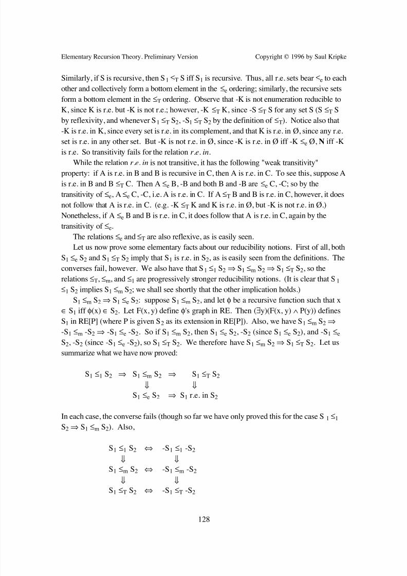
7/28/2019 Kripke Recursion Theory
http://slidepdf.com/reader/full/kripke-recursion-theory 132/191
Elementary Recursion Theory. Preliminary Version Copyright © 1996 by Saul Kripke
128
Similarly, if S is recursive, then S1 ≤T S iff S1 is recursive. Thus, all r.e. sets bear ≤e to each
other and collectively form a bottom element in the ≤e ordering; similarly, the recursive sets
form a bottom element in the ≤T ordering. Observe that -K is not enumeration reducible toK, since K is r.e. but -K is not r.e.; however, -K ≤T K, since -S ≤T S for any set S (S ≤T S
by reflexivity, and whenever S1 ≤T S2, -S1 ≤T S2 by the definition of ≤T). Notice also that
-K is r.e. in K, since every set is r.e. in its complement, and that K is r.e. in Ø, since any r.e.
set is r.e. in any other set. But -K is not r.e. in Ø, since -K is r.e. in Ø iff -K ≤e Ø, N iff -K
is r.e. So transitivity fails for the relation r.e. in.
While the relation r.e. in is not transitive, it has the following "weak transitivity"
property: if A is r.e. in B and B is recursive in C, then A is r.e. in C. To see this, suppose A
is r.e. in B and B ≤T C. Then A ≤e B, -B and both B and -B are ≤e C, -C; so by the
transitivity of ≤e, A ≤e C, -C, i.e. A is r.e. in C. If A ≤T B and B is r.e. in C, however, it does
not follow that A is r.e. in C. (e.g. -K ≤T K and K is r.e. in Ø, but -K is not r.e. in Ø.)
Nonetheless, if A ≤e B and B is r.e. in C, it does follow that A is r.e. in C, again by the
transitivity of ≤e.
The relations ≤e and ≤T are also reflexive, as is easily seen.
Let us now prove some elementary facts about our reducibility notions. First of all, both
S1 ≤e S2 and S1 ≤T S2 imply that S1 is r.e. in S2, as is easily seen from the definitions. The
converses fail, however. We also have that S1 ≤1 S2 ⇒ S1 ≤m S2 ⇒ S1 ≤T S2, so the
relations ≤T, ≤m, and ≤1 are progressively stronger reducibility notions. (It is clear that S1
≤1 S2 implies S1 ≤m S2; we shall see shortly that the other implication holds.)
S1 ≤m S2 ⇒ S1 ≤e S2: suppose S1 ≤m S2, and let φ be a recursive function such that x∈ S1 iff φ(x) ∈ S2. Let F(x, y) define φ's graph in RE. Then (∃y)(F(x, y) ∧ P(y)) defines
S1 in RE[P] (where P is given S2 as its extension in RE[P]). Also, we have S1 ≤m S2 ⇒-S1 ≤m -S2 ⇒ -S1 ≤e -S2. So if S1 ≤m S2, then S1 ≤e S2, -S2 (since S1 ≤e S2), and -S1 ≤e
S2, -S2 (since -S1 ≤e -S2), so S1 ≤T S2. We therefore have S1 ≤m S2 ⇒ S1 ≤T S2. Let us
summarize what we have now proved:
S1 ≤1 S2 ⇒ S1 ≤m S2 ⇒ S1 ≤T S2
⇓ ⇓S1 ≤e S2 ⇒ S1 r.e. in S2
In each case, the converse fails (though so far we have only proved this for the case S1 ≤1
S2 ⇒ S1 ≤m S2). Also,
S1 ≤1 S2 ⇔ -S1 ≤1 -S2
⇓ ⇓S1 ≤m S2 ⇔ -S1 ≤m -S2
⇓ ⇓S1 ≤T S2 ⇔ -S1 ≤T -S2
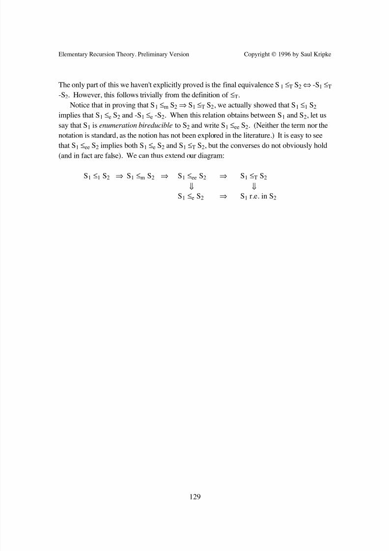
7/28/2019 Kripke Recursion Theory
http://slidepdf.com/reader/full/kripke-recursion-theory 133/191
Elementary Recursion Theory. Preliminary Version Copyright © 1996 by Saul Kripke
129
The only part of this we haven't explicitly proved is the final equivalence S1 ≤T S2 ⇔ -S1 ≤T
-S2. However, this follows trivially from the definition of ≤T.Notice that in proving that S1 ≤m S2 ⇒ S1 ≤T S2, we actually showed that S1 ≤1 S2
implies that S1 ≤e S2 and -S1 ≤e -S2. When this relation obtains between S1 and S2, let us
say that S1 is enumeration bireducible to S2 and write S1 ≤ee S2. (Neither the term nor the
notation is standard, as the notion has not been explored in the literature.) It is easy to see
that S1 ≤ee S2 implies both S1 ≤e S2 and S1 ≤T S2, but the converses do not obviously hold
(and in fact are false). We can thus extend our diagram:
S1 ≤1 S2 ⇒ S1 ≤m S2 ⇒ S1 ≤ee S2 ⇒ S1 ≤T S2
⇓ ⇓S1 ≤e S2 ⇒ S1 r.e. in S2

7/28/2019 Kripke Recursion Theory
http://slidepdf.com/reader/full/kripke-recursion-theory 134/191
Elementary Recursion Theory. Preliminary Version Copyright © 1996 by Saul Kripke
130
Lecture XVIII
Recursive Union.
We will now show how the notion of enumeration reducibility to a relation, or to a function,
can be reduced to the notion of enumeration reducibility to a set. In fact, the most obvious
thing works here: if R is an n-place relation and S is a set, let R' = {[x1, ..., xn]: R(x1, ...,
xn)}; then S ≤e R iff S ≤e R'. Similarly, if φ is a total n-place function and F = {[x1, ..., xn,
y]: φ(x1, ..., xn) = y}, then S ≤e φ iff S ≤e F. To show this is simply to show that the
languages RE[P11] and RE[Pn
1] (resp. RE[f n1]) have the same expressive power, where Pn1 is
interpreted as the relation R (resp. f n1 is interpreted as the function φ), and P11 is interpreted
as the set R' (resp. as the set F). To show this, we simply show how a formula in either
language can be translated into the other language. For simplicity, we concentrate on the
case of the 2-place relation R. If A is a formula of RE[P21], let A* be the formula of RE[P1
1]
that comes from A by replacing all occurrences of P21(x, y) by P1
1([x, y]); and if B is a
formula of RE[P11], let B† be the formula of RE[P2
1] that comes from B by replacing all
occurrences of P11(x) by (∃y)(∃z)(x = [y, z] ∧ P1
1(y, z)). It then suffices to check that A is
equivalent to A* and that B is equivalent to B†.
We can use this result to show that being r.e. in a relation or function (resp. Turing
reducibility to a relation or function) reduces to being r.e. in (resp. Turing reducibility to) a
set. Again, we focus on binary relations for simplicity. Suppose S is r.e. in R; then S ≤e R,-R, and the above proof will show that S ≤e R', -R', so S is r.e. in R'; the converse is proved
similarly. (Matters are a bit delicate here, since -(R') is not the same set as (-R)'; so we
really have to show that S ≤e R', (-R)' iff S ≤e R', -R'.) Now suppose S ≤T R. Then both S
and -S are r.e. in R, and so, as we have just seen, both S and -S are r.e. in R', so S ≤T R'.
Again, the converse is proved similarly.
We can also show that reducibility to several sets is nothing over and above reducibility
to a single set. What we really want is a pairing function on sets; if π is such a function,
then we want to show that S ≤e S1, S2 iff S ≤e π(S1, S2). (This is analogous to our use of a
recursive pairing function on numbers to reduce relations and functions to sets.) In fact, we
do have a suitable pairing function. For any sets S1 and S2, we define the recursive union
of S1 and S2 (written S1 U S2) to be the set {2n: n ∈ S1} ∪ {2n + 1: n ∈ S2}. It is easy to
verify that the function U is indeed a pairing function on sets of natural numbers. In fact, it
is an onto pairing function, i.e. every set S is S1 U S2 for some S1 and S2. S1 and S2 are
called the even and odd parts of S, respectively.
The idea behind recursive union is one that is familiar from other branches of
mathematics: S1 U S2 is the union of disjoint copies of S1 and S2. It is different from
ordinary unions in the following striking way: whereas -(S1 ∪ S2) = -S1 ∩ -S2, -(S1 U S2)
= -S1 U -S2. (Proof: the even part of -(S1 U S2) is {n: 2n ∈ -(S1 U S2)} = {n: 2n ∉ (S1 U

7/28/2019 Kripke Recursion Theory
http://slidepdf.com/reader/full/kripke-recursion-theory 135/191
7/28/2019 Kripke Recursion Theory
http://slidepdf.com/reader/full/kripke-recursion-theory 136/191
Elementary Recursion Theory. Preliminary Version Copyright © 1996 by Saul Kripke
132
Let us now verify two important properties of enumeration operators. The first is
monotonicity. An operator ψ is said to be monotonic if whenever S1 ⊆ S2, ψ (S1) ⊆ ψ (S2).
(When ψ takes as its values the truth values T and F, then we say that ψ is monotonic if whenever S1 ⊆ S2 and ψ (S1) = T, then ψ (S2) = T.) The second is finiteness. An operator is
said to be finite if for all x and S, x ∈ ψ (S) iff there is some finite S0 ⊆ S such that x ∈ψ (S0).
Once we have proved monotonicity and finiteness for the case k = 0, the result will
follow for all k > 0. To see this, suppose ψ is an enumeration operator corresponding to a
formula A(x1, ..., xn) of RE[P], and suppose S1 ⊆ S2. Suppose <a1, ..., an> ∈ ψ (S1). Then
<a1, ..., an> satisfies A(x1, ..., xn) when P is interpreted as S1, so the sentence A(0(a1), ...,
0(an)) of RE[P] is true. By monotonicity for k = 0, A(0(a1), ..., 0(an)) remains true when P
is interpreted as S2, and so <a1, ..., an> still satisfies A(x1, ..., xn), i.e. <a1, ..., an> ∈ ψ (S2).
Since the n-tuple <a1, ..., an> was arbitrary, it follows that ψ (S1) ⊆ ψ (S2). Similarly,
suppose finiteness holds for the case k = 0, and suppose <a1, ..., an> ∈ ψ (S). Then <a1, ...,
an> satisfies A(x1, ..., xn) when P is interpreted as S, so A(0(a1), ..., 0(an)) is true; by
finiteness, A(0(a1), ..., 0(an)) is true when P is interpreted as S0 for some finite S0 ⊆ S, so
<a1, ..., an> ∈ ψ (S0).
Theorem: Monotonicity holds for enumeration operators.
Proof : By the foregoing discussion, we need only show that if A is a sentence of RE[P]
and A is true when P is interpreted as S1, then A remains true when P is interpreted as S2
whenever S1 ⊆ S2. (To save words, let us say that A is true in S to mean that A is true whenP is interpreted as S.) We show this by induction on the complexity of RE[P] sentences.
Atomic sentences are either sentences of RE or sentences of the form P(0(n)). The former
are true or false independently of how P is interpreted, and P(0(n)) is true in S iff n ∈ S, so
obviously the theorem holds for P(0(n)). If the theorem holds for A and B, and A ∧ B is
true in S1, then both A and B are true in S1 and by the inductive hypothesis remain true in
S2; therefore, A ∧ B is true in S2. The remaining cases offer no difficulty and are left to the
reader.
Theorem: Finiteness holds for enumeration operators.
Proof : Again, we only have to show that a sentence A of RE[P] is true when P isinterpreted as some set S iff A is true when P is interpreted as S0 for some finite S0 ⊆ S.
The "if" part is trivial, by monotonicity. We prove the "only if" part by induction on the
complexity of sentences. If a sentence is atomic, it is either a sentence of RE or of the form
P(0(n)). In the former case, the interpretation of P is irrelevant to its truth, so we can take S0
= Ø. In the latter case, if P(0(n)) is true in S, then n ∈ S, so we can take S0 = {n}.
If A ∨ B is true in S, then either A or B is true in S; suppose A is. Then by the inductive
hypothesis, A is true in S0 for some finite S0 ⊆ S, so the sentence A ∨ B is also true in S0.
If A ∧ B is true in S, then both A and B are true in S, so by the inductive hypothesis
7/28/2019 Kripke Recursion Theory
http://slidepdf.com/reader/full/kripke-recursion-theory 137/191
Elementary Recursion Theory. Preliminary Version Copyright © 1996 by Saul Kripke
133
there are finite sets S1, S2 ⊆ S such that A and B are true in S1 and S2, respectively. So by
monotonicity, both A and B are true in the finite set S0 = S1 ∪ S2, and so A ∧ B is true in
S0.If (∃x)A(x) is true in S, then the case is like disjunction. A(0(n)) is true for some n, so
by the inductive hypothesis A(0(n)) is true in S0 for some finite S0 ⊆ S; so (∃x)A(x) is true
in S0.
If (x < 0(n))A(x) is true in S, then the case is like conjunction. A(0), ..., A(0(n-1)) are all
true in S, so by the inductive hypothesis they are true in finite sets S1, ..., Sn, respectively.
So by monotonicity, they are all true in the finite set S0 = S1 ∪ ... ∪ Sn. So the sentence (x
< 0(n))A(x) is itself true in S0.
The set S0 is sometimes called a finite support for the sentence.
We can use the last theorem to prove a normal form theorem for sentences or RE[P].
Let A be such a sentence. A is true in S iff for some finite S0 ⊆ S, A is true in S0. (And by
the discussion above, this also holds if A has free variables.) We can write out the right side
of the "iff" in RE[P]. Let s be some variable that does not occur in A, and let A* be the
result of replacing all occurrences of P(t) by t ∈ s, for t a term. A* is thus a formula of RE.
Let s ⊆ P abbreviate the RE[P] formula (x < s)(x ∉ s ∨ P(x)). Then A is equivalent to the
formula (∃s)(s ⊆ P ∧ A*). Thus, the extra predicate P can be segregated off, as it were, so
that it only occurs in the conjunct s ⊆ P.
The normal form theorem gives us an enumeration theorem: to get an enumeration of
the n-place relations definable in RE[P], we simply replace A* by the formula W(e, s, x1, ...,xn). If an n-place relation R is definable in RE[P], then it is definable by a normal form
formula (∃s)(s ⊆ P ∧ A*(x1, ..., xn)), and A*(x1, ..., xn) is equivalent to W(0(e), s, x1, ..., xn)
for some e, so R is defined by the formula (∃s)(s ⊆ P ∧ W(0(e), s, x1, ..., xn)); so (∃s)(s ⊆P ∧ W(e, s, x1, ..., xn)) (in which e is now a variable) defines an n+1-place relation that
enumerates the n-place relations definable in RE[P], since R was arbitrary. (e is an index of
the relation R here.) In fact, this also gives us an enumeration of the enumeration operators;
we will sometimes write ψ e to denote the eth operator in this enumeration. (We could have
also proved an enumeration theorem by imitating the proof of the enumeration theorem for
RE.)
The Enumeration Operator Fixed-Point Theorem.
We shall now prove that every enumeration operator has a least fixed point, and that this
fixed point is r.e. This theorem is closely related to Kleene's first recursion
theorem.Kleene stated his first recursion theorem in terms of partial recursive functions, but,
just as in the case of the second recursion theorem, we first give the version for r.e. sets and
relations. We will consider Kleene's form of the theorem at the end of the section.
7/28/2019 Kripke Recursion Theory
http://slidepdf.com/reader/full/kripke-recursion-theory 138/191
Elementary Recursion Theory. Preliminary Version Copyright © 1996 by Saul Kripke
134
A fixed point of a function φ is an x such that φ(x) = x, so in particular a fixed point of
an enumeration operator ψ is a set S such that ψ (S) = S. A set S is said to be closed (under
ψ ) if ψ (S) ⊆ S. S is said to be sound if S ⊆ ψ (S). So S is fixed iff S is both sound andclosed. If S is a fixed point of ψ , we say that S is the least fixed point of ψ if S ⊆ S' for all
fixed points S' of ψ .
Theorem: Every monotonic operator has a least fixed point.
Proof : We shall give two proofs of this theorem; the first is shorter, but the second gives us
more information about the least fixed point, and this information will be useful later.
Let G = ∩{S: S is closed}. ({S: S is closed} is not empty, since we know that there is
at least one closed point, namely N.) First, we show that G is closed. If S is closed, then G
⊆ S by the definition of G, so ψ (G) ⊆ ψ (S) ⊆ S by ψ 's monotonicity and S's closedness.
So ψ (G) ⊆ S for all closed S, and therefore ψ (G) ⊆ G by the definition of G, and G is
closed. Next, we show that G is sound. Note that ψ (G) is closed: ψ (G) ⊆ G as we have
seen, so ψ (ψ (G)) ⊆ ψ (G) by monotonicity. Since ψ (G) is closed, G ⊆ ψ (G), so G is
sound. So G is a fixed point. Finally, G is the least fixed point: if S is a fixed point, then S
is closed, so G ⊆ S by the definition of G.
In the second proof, we construct a fixed point by transfinite induction. Let S0 = Ø, and
for all n, let Sn+1 = ψ (Sn). After we have constructed Sn for all n ∈ N, we let Sω = ∪{Sn: n
∈ N}. In general, if Sα has been defined, we set Sα+1 = ψ (Sα), and if α is a limit ordinal
(i.e. an ordinal which is not β+1 for any β), we set Sα = ∪{Sβ: β < α}. We show by
induction on α that Sα is sound for all α; given the definition of Sα, this means that Sα
⊆Sα+1. Clearly, S0 is sound. If Sα is sound, i.e. Sα ⊆ Sα+1, then ψ (Sα) ⊆ ψ (Sα+1) by
monotonicity, i.e. Sα+1 ⊆ Sα+2. Now let α be a limit ordinal, and suppose Sβ is sound for
all β < α. Let x ∈ Sα. By the definition of Sα, x ∈ Sβ for some β < α, and Sβ ⊆ Sα. By
monotonicity, ψ (Sβ) ⊆ ψ (Sα) = Sα+1, and by the inductive hypothesis Sβ ⊆ ψ (Sβ), so x ∈Sα+1. Since x was arbitrary, Sα ⊆ Sα+1.
So the sequence <Sα: α an ordinal> is increasing. It can't be strictly increasing, since if
it were, a new natural number would be added to Sα at each stage; so at an uncountable
stage, uncountably many natural numbers would have been added, which is impossible.
(We can make this precise, as follows. If Sα ≠ Sα+1 for each α, then Sα+1 - Sα must be
nonempty for each α, so let φ(α) be the least element of Sα+1 - Sα. Then φ is a 1-1 functionfrom the ordinals into N. So if α is an uncountable ordinal, then φ maps {β: β < α} 1-1
into N, which is impossible.) So the sequence must stop increasing eventually, that is there
must be a λ such that Sλ = Sλ +1; indeed there must be a countable such λ . But this means
that ψ (Sλ ) = Sλ , i.e. Sλ is a fixed point of ψ .Finally, we can show that Sλ is the least fixed point by showing, by ordinal induction on
α, that if S' is any fixed point, then Sα ⊆ S'; it follows that Sλ ⊆ S'.

7/28/2019 Kripke Recursion Theory
http://slidepdf.com/reader/full/kripke-recursion-theory 139/191
Elementary Recursion Theory. Preliminary Version Copyright © 1996 by Saul Kripke
135
Exercises
1. Show that for all sets S, S1, and S2, S ≤e S1, S2 iff S ≤e S1 U S2.
2. Suppose S is a completely creative set, and let ψ be a completely creative function for S
(i.e. for all x, ψ (x) ∈ S iff ψ (x) ∈ Wx). First, show that there is a recursive function χ1
such that Wχ1(x, s) = Wx - {a1, ..., an}, where s codes {a1, ..., an}, and a recursive function χsuch that Wχ(x, y) = Wx ∪ {y}. Next, define α and ψ * simultaneously, as follows. α(n, 0)
= χ1(n, s), where s is the smallest code of {ψ *(0), ..., ψ *(n-1)}; α(n, m+1) = χ(α(n, m),
ψ (α(n, m))); ψ *(0) = ψ (0); and ψ *(n+1) = ψ (α(n+1, q0)), where q0 is the least q such that
ψ (α(n+1, q)) is distinct from all of ψ *(0), ..., ψ *(n). Prove that ψ * is total recursive, 1-1,
and a completely creative function for S.
Use this and previous exercises to show that the notions 1-complete, m-complete,
creative, 1-1 creative, completely creative, 1-1 completely creative and being an r.e.
nonrecursive set satisfying the effective form of Gödel’s theorem are all equivalent.
Remark: remember that I said that r.e. sets that arise naturally, as opposed to being
cooked up by recursion theorists, are all either recursive or 1-1 complete. The latter case can
be characterized in all the ways on the list above.
3. Use the method of axiomatizing in first-order logic, as given in class, to show that all
Turing-computable functions are recursive.
4. Recall the self-reference lemma with parameters from class: if A(x) is any formula, there
is a recursive function ψ and a formula PS(x, y) that represents ψ in Q, such that for all m,
ψ (m) is the Gödel number of the formula (∃z)(PS(0(m), z) ∧ A(z)), which is provably
equivalent in Q to A(0(ψ (m))). Use this to prove that every r.e. set is nicely weakly
representable in every consistent r.e. extension of Q, as follows. Let Γ be any consistent r.e.
extension of Q and let S be any r.e. set. Let R(x, y) be a formula of Lim such that the
formula (∃y)R(x, y) defines S. Let Pr(x, y) be a formula of Lim such that (∃y)Pr(x, y)
defines the set of theorems of Γ . Let A(x) be the formula (∃z)(PS(x, z) ∧ (∃y)(R(x, y) ∧ (w
< y)~Pr(z, w))), where PS represents the function ψ such that ψ (m) is the Gödel number of
the formula A(0(m)). Show that A(x) weakly represents S in Γ , and moreover that A(x)defines S.
Remark: a previous exercise proved that every r.e. set is weakly representable in every
consistent extension of Q, but not that the weak representation was nice. Shepherdson gave
this as an alternative way of getting the earlier result, and then Kreisel pointed out that this
method gives a nice weak representation.
5. Consider the language that is like RE except that the bounded universal quantifier is
replaced by the ordinary unbounded universal quantifier. This can be called the positive
7/28/2019 Kripke Recursion Theory
http://slidepdf.com/reader/full/kripke-recursion-theory 140/191
Elementary Recursion Theory. Preliminary Version Copyright © 1996 by Saul Kripke
136
language of arithmetic, PL.
(a) Prove that the same sets and relations are definable in the (ordinary) language of
arithmetic, L, as are definable in PL.Now consider the language PL[P1
1] obtained by adding to PL a single monadic predicate
P11, just as in the case of RE. Analogously to enumeration operators, we can define positive
arithmetical operators. Also, let φ(S) be the set of all (Gödel numbers of) true sentences of
PL[P11], where the extra predicate P1
1 is interpreted as S.
(b) Show that in contrast to the case of RE[P11], φ(S) is not a positive arithmetical
operator. Also show that every enumeration operator is a positive arithmetical operator.
Show as well that positive arithmetical operators need not in general be finite.
(c) Prove that φ(S) is monotonic, and show how to deduce that every positive
arithmetical operator is monotonic.
(d) In class it was proved that every monotonic operator has a least fixed point. Prove
the following statements by similar methods: every monotonic operator has a unique largest
fixed point. Also, for every monotonic operator, every sound point S has a least fixed point
above S, and every closed point S has a largest fixed point below S.
Notice that by (c) the conclusions of (d) apply to φ and to every positive arithmetical
operator. In particular, they all have least fixed points and largest fixed points.
(e) If P11 is interpreted by any fixed point of φ, show that the language PL[P1
1] contains
its own truth predicate and its own satisfaction predicates Satk(x, m1,...,mk), for each k.
(f) The self-reference lemma for the language PL[P11] (for the case of formulae with one
free variable) says that for any formula of this language A(x1), with only x1 free and x1never bound, there is a formula G with Gödel number m such that, independently of the
interpretation of the extra predicate P11, G≡A(0(m)) is always provable from the axioms of
Q, if we consider the theorems of Q derivable in the broad language of arithmetic
supplemented by the predicate P11. A corollary is that G≡A(0(m)), where m is the Gödel
number of G, is always true, regardless of how the extra predicate is interpreted. Prove the
self-reference lemma for PL[P11]. (In fact, all the forms of the self-reference lemma proved
in class for the language of arithmetic generalize over to this case in a similar manner.
However, here we only consider the form of the lemma we need for part (g).)
(g) Consider a sentence G such that G≡P11(0(m)) (where m is the Gödel number of G)
is true, regardless of the interpretation of P11. Such a sentence exists by (f). Prove that thereis at least one fixed point S1 of φ such that if P1
1 is interpreted by S1, G is true, and another
fixed point S2 such that if P11 is interpreted by S2, G is false. Prove that G is true if P1
1 is
interpreted by the largest fixed point of φ and false if P11 is interpreted by the least fixed
point of φ. (This shows that there are at least two distinct fixed points and that in fact the
largest and the least fixed points are distinct. In fact, the number of fixed points is the
cardinality of the continuum.)
Remark: this finally shows that a language even with unbounded quantifiers of both
7/28/2019 Kripke Recursion Theory
http://slidepdf.com/reader/full/kripke-recursion-theory 141/191
Elementary Recursion Theory. Preliminary Version Copyright © 1996 by Saul Kripke
137
kinds, and with an expressive power greater than or equal to the language of arithmetic, can
express its own truth and satisfaction predicates, as long as it lacks negation. Any
interpretation of P11 in PL by a fixed point has these properties. We have seen that there is
more than one such interpretation of P11. The same argument could be used for RE[P1
1], but
it is less interesting there, because all the languages RE[P11], and RE itself, contain their own
truth and satisfaction predicates.
The construction is related to one I have discussed elsewhere, but differs in that it is for
classical languages without negation.
7/28/2019 Kripke Recursion Theory
http://slidepdf.com/reader/full/kripke-recursion-theory 142/191
Elementary Recursion Theory. Preliminary Version Copyright © 1996 by Saul Kripke
138
Lecture XIX
The Enumeration Operator Fixed-Point Theorem (Continued)
We could adapt either proof that every monotonic operator has a least fixed point to give us
additional information. For example, for any sound point S, there is a least fixed point S'
such that S ⊆ S'. We can show this either by letting G = ∪{S': S' is closed and S ⊆ S'} in
the first proof, or by letting S0 = S in the second proof. Also, for any closed point S', there
is a greatest fixed point S ⊆ S'. Again, we can imitate the first proof (switching "closed"
and "sound" and making similar changes throughout) or fiddle with the second proof
(letting <Sα> be a decreasing sequence with S0 = S).
In the second proof, we know that a fixed point is reached at some countable stage. If
the operator ψ is finite, then it is reached at stage ω .
Theorem: If ψ is a monotonic and finite operator, then the set Sω from the proof of the last
theorem is ψ 's least fixed point.
Proof : We only have to show that Sω = Sω +1; since Sω ⊆ Sω +1, we just have to show that
Sω +1 ⊆ Sω . Let x ∈ Sω +1 = ψ (Sω ). By finiteness, we can find a finite X ⊆ Sω such that x
∈ ψ (X). Since X is finite, X ⊆ Sn for some n < ω . By monotonicity, x ∈ ψ (Sn). But Sn+1
= ψ (Sn), so x ∈ Sn+1 ⊆ Sω .
Since enumeration operators are finite and monotonic, we know already that each
enumeration operator has a least fixed point, and that it is constructed by stage ω . To show
that this fixed point is r.e., we need to generalize the generated sets theorem slightly.
When a set is generated from a basis set and a collection of rules in the sense of the
usual generated sets theorem, the rules are finite in number and each has a fixed finite
number of premises. However, since we can code up finite sets of numbers as individual
numbers, we can make sense of an r.e. generating rule having a variable finite number of
premises. Specifically, we can identify such a rule with a binary relation R(s, x), where s
codes a finite set of premises and x is the conclusion. We can formulate an appropriatenotion of proof sequence for such a relation; specifically, we may say that <x1, ..., xn> is a
proof sequence for R if for every i≤n there is a finite set s such that all elements of s are in
<x1, ..., xn> before xi and R(s, xi). Then naturally we define the set generated by R to be the
set of all numbers that have proof sequences. As long as R is r.e., the notion of proof
sequence will be r.e., and therefore the set generated by R will also be r.e. We leave the
details to the reader.
Enumeration Operator Fixed Point Theorem: Every enumeration operator has a least
7/28/2019 Kripke Recursion Theory
http://slidepdf.com/reader/full/kripke-recursion-theory 143/191
Elementary Recursion Theory. Preliminary Version Copyright © 1996 by Saul Kripke
139
fixed point (namely Sω ), and that fixed point is r.e.
Proof : Let ψ be an enumeration operator, and let Sω be as above. Let R be the relation {<s,
x>: s codes a set S such that x ∈ ψ (S)}. R is r.e., as is easily seen (if A is the RE[P]formula corresponding to ψ , then R is defined by the formula A' obtained from A by
replacing P(t) by t ∈ s throughout). Let G be the set generated by R, which is therefore r.e.
We show that G = Sω .
First, G ⊆ Sω . We show by induction on the length of proof sequences that if x occurs
on a proof sequence, then x ∈ Sω . Let <x1, ..., xn> be a proof sequence for R. Then R(s,
xn), where s codes a finite set of xi's, i < n. By the inductive hypothesis, s codes a subset S
of Sω , so by monotonicity ψ (S) ⊆ ψ (Sω ) = Sω . Since xn ∈ ψ (S), xn ∈ Sω .
Next, Sω ⊆ G. We show by induction on n that Sn ⊆ G. S0 = Ø ⊆ G. Suppose Sn ⊆G, and let x ∈ Sn+1 = ψ (Sn). By finiteness, x ∈ ψ (S) for some finite S ⊆ Sn. Since Sn+1
⊆ G, we can find proof sequences for all the elements of S; by stringing them together, we
can find a proof sequence for x. So x ∈ G.
Kleene's first recursion theorem is stated in terms of partial recursive functions. An
enumeration operator that maps partial functions into partial functions is called a partial
recursive operator; Kleene showed that every partial recursive operator has a least fixed
point, and that this fixed point is a partial recursive function. We can prove this using the
enumeration operator fixed point theorem as follows. By identifying partial functions with
their graphs, and identifying relations with sets of coded pairs, we can see that any partial
recursive operator ψ has a least fixed point R, where R is an r.e. relation. To see that R issingle valued, we use the fact that R is Rω . R0 = Ø is single valued; if Rn is single valued,
then since y is a partial recursive operator, Rn+1 = ψ (Rn) is single valued; so each Rn is
single valued. Suppose [x, y] and [x, z] ∈ Rω . Then for some m, n, [x, y] ∈ Rm and [x, z]
∈ Rn. Let p = max(m, n); then [x, y], [x, z] ∈ Rp. Since Rp is single valued, y = z. So Rω
is single valued.
The First and Second Recursion Theorems.
Here are the two recursion theorems:
(1) For all enumeration operators ψ , there is a least set S such that ψ (S) = S, and moreover
S is r.e.
(2) For all recursive functions φ, there is an e such that We = Wφ(e).
Neither of these theorems implies the other. On the one hand, the second recursion theorem
implies that every enumeration operator has an r.e. fixed point, but not that it has a least
fixed point. To see this, let ψ be any enumeration operator, and let A be a formula of RE[P]
7/28/2019 Kripke Recursion Theory
http://slidepdf.com/reader/full/kripke-recursion-theory 144/191
Elementary Recursion Theory. Preliminary Version Copyright © 1996 by Saul Kripke
140
corresponding to it. Let A*(e, x) be the formula of RE obtained from A by replacing P(x)
by W(e, x) throughout. Then A*(e, x) defines the relation {<e, n>: n ∈ ψ (We)}, so that
relation is r.e. Using the Smn theorem, we can find a recursive function φ such that Wφ(e) =
ψ (We) for all e. To find an r.e. fixed point for ψ , apply (2) to find an e such that We =
Wφ(e) = ψ (We). We need not be the least fixed point, however.
On the other hand, we can use (1) to prove (2) only in a special case. Since the φ in (2)
is a function on numbers rather than sets, it is quite possible that We = Wf and Wφ(e) ≠Wφ(f) for some e and f; in that case, the "operator" F(We) = Wφ(e) will not even be well-
defined, let alone an enumeration operator. However, let us say that a function φ is
extensional if for all e and f, if We = Wf then Wφ(e) = Wφ(f). Then the operator F(We) =
Wφ(e) is well-defined. It turns out that whenever φ is extensional, there is an enumeration
operator ψ such that ψ (We) = Wφ(e) for all e. We can thus apply (1) to ψ to obtain an e
such that We = ψ (We) = Wφ(e).
If we only applied (2) with extensional φ in practice, then this would not be much of a
limitation. However, there are important applications of (2) in which φ is nonextensional, or
at least in which there is no good reason to think that φ is extensional; the study of recursive
ordinals is an example of this.
(1) and (2) have many applications in common. For example, we can use (1), as we
used (2), to prove that certain functions defined in terms of themselves are recursive. Take
the factorial function, for example. We can define a partial recursive operator as follows:
Ψ(φ) = χ, where χ(0) = 0 and χ(n+1) = φ(n).(n+1). It is easy to check that Φ is a partial
recursive operator; applying the version of (1) for such operators, we see that there is apartial recursive φ such that Ψ(φ) = φ, so that φ(0) = 0 and φ(n+1) = φ(n).(n+1), i.e. φ(n) =
n! for all n. (In fact, this proof that the factorial function is recursive boils down to the
proof we gave earlier in terms of the generated sets theorem; the operator Ψ is really a kind
of generating rule.) (1) and (2) are called recursion theorems because of these common
applications.
The Intuitive Reasons for Monotonicity and Finiteness.
We have shown, in terms of our formalism, that enumeration operators are monotone andfinite; we can also give intuitive proofs of the corresponding claims about the intuitive
notion of semi-computability. Let P be a semi-computation procedure which consults an
oracle; let us say that P semi-computes a set S1 from S2 if, whenever P is given an oracle to
S2, it answers "yes" to input n iff n ∈ S1. In this case, let us write S1 = P(S2). We want to
show that if S1 ⊆ S2 then P(S1) ⊆ P(S2), and that if n ∈ P(S), then n ∈ P(S0) for some
finite S0 ⊆ S.
Suppose n ∈ P(S1). Then whenever P is given an oracle to S1 and gets input n, P halts
after a finite amount of time with answer "yes". Since P halts after a finite amount of time,
7/28/2019 Kripke Recursion Theory
http://slidepdf.com/reader/full/kripke-recursion-theory 145/191
Elementary Recursion Theory. Preliminary Version Copyright © 1996 by Saul Kripke
141
P only asks the oracle finitely many questions, so a finite amount of information about S1
suffices for P to decide that n ∈ P(S1). Moreover, this information is positive information,
since the oracle only gives "yes" answers to P's questions. Let S0 = {x ∈ S1: the oraclegives an answer "yes" to the question "x ∈ S1?"}; then S0 is finite, S0 ⊆ S1, and the
information in S0 suffices for P to decide that n ∈ P(S1). It follows that n ∈ P(S0) and that
n ∈ P(S2) when S1 ⊆ S2: if P is given an oracle to the set S0 (or S2) and given input n,
then it will proceed as it did when given an oracle to S1, asking it exactly the same questions,
and it will get the same "yes" answers, which suffice to make P halt and give an answer
"yes".
We can use this fact to prove a normal form theorem for semi-computability. If S1 is
semi-computable in a semi-computation of S2, then S1 = P(S2) for some P, and by our
monotonicity and finiteness result, n ∈ P(S2) iff n ∈ P(S0) for some finite S0 ⊆ S2. Now,
the relation n ∈ P(S0) (holding between n and S0) is clearly a semi-computable relation,
since we can transform P into a procedure P* that semi-computes it: whenever P consults
the oracle about whether n is an element of the set in question, let P* invoke a semi-
computation procedure for the relation n ∈ S0. Note that P* is a semi-computation
procedure without oracles. We have thus shown that whenever a set S1 is semi-computable
in a semi-computation of S2, there is a semi-computable relation R such that S1 = {n: (∃finite S0)(S0 ⊆ S2 ∧ R(n, S0))}. If the unrelativized version of Church's thesis is true, then
R must be r.e., and therefore there is an r.e. relation such that S1 = {n: (∃ finite S0)(S0 ⊆ S2
∧ R(n, S0))}. But this holds precisely when S1 ≤e S2. So the unrelativized version of
Church's thesis implies the relativized version.
Degrees of Unsolvability.
Suppose a binary relation ≤ is reflexive and transitive; then the relation ≡, defined by a ≡ b
iff a ≤ b and b ≤ a, is an equivalence relation. To verify this, we must show that ≡ is
reflexive, symmetric, and transitive. That ≡ is symmetric is immediate from the definition
and does not depend on any properties of ≤. ≡'s reflexivity follows from that of ≤. Finally,
if a ≡ b and b ≡ c, then a ≤ b and b ≤ c by the definition of ≡, so a ≤ c by ≤'s transitivity, and
similarly c ≤ a, so a ≡ c. We have shown that all of our reducibility notions are reflexiveand transitive, so in each case the relation of interreducibility is an equivalence relation. We
write A ≡e B for A ≤e B & A ≤e B, and similarly for ≡1, ≡m, and ≡T. The equivalence
classes are called degrees of unsolvability, or simply degrees. In particular, the ≡e-, ≡1-, ≡m-
and ≡T- equivalence classes are called enumeration degrees, 1-degrees, m-degrees, and
Turing degrees, respectively. (We use lowercase letters to denote degrees.) The idea
behind this terminology is that when a set A is reducible to a set B, B is harder to compute
than A, i.e. the decision problem for B has a higher degree of difficulty than that of A. (Or
the semi-decision problem, in the case of enumeration degrees.) Degrees, especially Turing
7/28/2019 Kripke Recursion Theory
http://slidepdf.com/reader/full/kripke-recursion-theory 146/191

7/28/2019 Kripke Recursion Theory
http://slidepdf.com/reader/full/kripke-recursion-theory 147/191
Elementary Recursion Theory. Preliminary Version Copyright © 1996 by Saul Kripke
143
behind our definition of * is that S* encodes an enumeration of all the sets ≤e S; to get this
effect, we could have taken S* to be {[e, m]: m satisfies the formula of RE[P] whose Gödel
number is e}. Or, since we can reduce satisfaction to truth, we could have taken S* to bethe set of Gödel numbers of true sentences of RE[P]. Both of these sets are recursively
isomorphic to S* as we actually defined it.
Another important equivalence involving * is the following:
A ≤e B ⇔ A* ≤1 B*.
For suppose A ≤e B. Then since A ≡e A* and B ≡e B*, A* ≤e B*; but then A* ≤1 B*. On
the other hand, suppose A* ≤1 B*. Then A* ≤e B by the equivalences for *, and so A ≤e B
since A ≡e A*.
While S* is always ≤e S, -S* is never ≤e S. The proof is analogous to the proof that K
is not recursive. Suppose -S* ≤e S, and let A = {m: [m, m] ∉ S*}; A ≤e -S*, so by the
transitivity of ≤e, A ≤e S. A has some index e; so for all m, m ∈ A iff [e, m] ∈ S*, and in
particular, e ∈ A iff [e, e] ∈ S*; but e ∈ A iff [e, e] ∉ S* by the definition of A,
contradiction.
We now define S' to be the set (S U -S)*. S' is called the jump of S. (While the
operation * is not a standard part of recursion theory, the jump operation is very standard.)
Just as S* ≤e S, S' is r.e. in S: (S U -S)* ≤e S U -S by the properties of *, i.e. (S U -S)* is
r.e. in S, i.e. S' is r.e. in S. However, -S' is never r.e. in S: if -S' is r.e. in S, then -(S U -S)*
≤e SU
-S, which we have just seen to be impossible. So S' is never recursive in S.However, S ≤T S': by the basic properties of *, (S U -S) ≤e (S U -S)*, so S ≤e S' and -S ≤e
S'. So S' is always of a higher Turing degree than S.
As in the case of *, the exact definition of ' is less important than its basic properties.
We could have defined S' to be {[e, m]: m satisfies the formula of RE[P1, P2] with Gödel
number e}, where P1 and P2 are interpreted as S and -S, respectively. We could also have
defined S' to be the diagonal set {e: e satisfies the formula of RE[P1, P2] with Gödel
number e}. In this way, we see that S' can be viewed as a relativization of K to the set S.
As with *, we have the following equivalences involving ':
A ≤1 S' ⇔ A ≤m S' ⇔ A ≤e S' ⇔ A is r.e. in S.
In general, we will forget about the definition of ' and work directly from these equivalences.
Since A is r.e. in S iff A ≤e S U -S, this follows directly from our equivalences for * by
replacing S by S U -S.
We also have the following:
A ≤T B ⇔ A' ≤1 B' ⇔ A' ≤m B' ⇔ A' ≤e B'.
7/28/2019 Kripke Recursion Theory
http://slidepdf.com/reader/full/kripke-recursion-theory 148/191

7/28/2019 Kripke Recursion Theory
http://slidepdf.com/reader/full/kripke-recursion-theory 149/191
Elementary Recursion Theory. Preliminary Version Copyright © 1996 by Saul Kripke
145
Lecture XX
More on the Jump Operator.
As we have seen, there is a least T-degree, namely 0, the set of all recursive sets. Using the
jump operator, we can form an increasing sequence of degrees: 0, 0', 0'', .... In general, we
write 0(n) (the nth jump of 0) for the result of applying ' to 0 n times. We know that this
sequence is strictly increasing, i.e. 0 < 0' < 0'' ..., since A' is never recursive in A.
If a and b are degrees, where a = deg(A) and b = deg(B), we define a ∪ b to be deg(A U
B). For any of the four kinds of degrees we have been considering, a ∪ b is well-defined
and is an upper bound of a and b (i.e. a, b ≤ a ∪ b). Moreover, if a and b are either Turing
or enumeration degrees, a ∪ b is the least upper bound of a and b, i.e. for all degrees c, if a,
b ≤ c, then a ∪ b ≤ c.
First, let us verify that a ∪ b is well defined, i.e. that the degree of A U B does not
depend on which sets A and B we pick from the degrees a and b. That is, we must show
that if A ≡r A1 and B ≡r B1, then A U B ≡r A1 U B1 (for r = 1, m, T, e). We assume that A
≡r A1 and B ≡r B1, and show that A U B ≤r A1 U B1 (as the proof that A1 U B1 ≤r A U B
will be exactly the same). We know already from our previous work that A U B ≤T A1 U B1
iff both A and B are ≤T A1 U B1, iff both A and B are ≤T A1, B1. But A ≤T A1, B1 since A
≤T A1 by hypothesis, and similarly B ≤T A1, B1. The same holds for ≤e. So consider the
case r = m. A ≤m A1 and B ≤m B1, so let φ and ψ be recursive functions such that φ: A ≤mA1 and ψ : B ≤m B1. Let χ be the recursive function such that χ(2n) = 2φ(n) and χ(2n+1) =
2ψ (n)+1; χ: A U B ≤m A1 U B1. Finally, if φ and ψ are 1-1, then χ is also 1-1, so A U B ≤1
A1 U B1.
Next, since A U B is an upper bound of A and B in all of our reducibility notions,
Degr(A) and Degr(B) are ≤ Degr(A U B) for all A and B, i.e. a, b ≤ a ∪ b. Finally, as we
saw, A, B ≤T, e C implies A U B ≤T, e C, so a, b ≤ c implies a ∪ b ≤ c if a, b, and c are
enumeration degrees or Turing degrees.
We say that a partially ordered set is an upper semilattice if any two elements of it have
a least upper bound, and a lower semilattice if any two elements have a greatest lower
bound. A partially ordered set which is both an upper and a lower semilattice is called alattice. Thus, we see that the degrees form an upper semilattice; however, it turns out that
they do not form a lower semilattice, and hence do not form a lattice.
It is easy to check that the operator ∪ is associative and commutative, and that for all a1,
..., an, a1 ∪ ... ∪ an is the least upper bound of a1, ..., an. (These facts depend only on the
fact that a ∪ b is the least upper bound of a and b.) Thus, any finite set of degrees has a
least upper bound. It does not follow, however, that every set of degrees has a least upper
bound. In fact, this is not the case: if F is a family of degrees, then for F to have a least
upper bound, it is necessary and sufficient that there be a finite E ⊆ F such that for all a ∈ F
7/28/2019 Kripke Recursion Theory
http://slidepdf.com/reader/full/kripke-recursion-theory 150/191
Elementary Recursion Theory. Preliminary Version Copyright © 1996 by Saul Kripke
146
there is a b ∈ E with a ≤ b. Thus, in particular, the sequence 0, 0', 0'', ... has no least upper
bound, since no such E exists.
Notice that 0' is the degree of Ø' (since 0 is the degree of Ø), and that Ø' is a 1-1complete set. To see this, note that Ø' = (Ø U N)* = {odds}* = {[e, m]: (∃s)(s ⊆ {odds}
∧ W(e, m, s))}; so if A is any r.e. set, the relation R given by R(x, y) iff x ∈ A ∧ y ∈ N is
r.e., and therefore has an index e: so for all m, m ∈ A iff for some (or any) s, R(m, s), iff
W(e, m, s) for some such s, iff [e, m] ∈ Ø'. So A ≤1 Ø' by the map m → [e, m]. Thus, we
see that 0' is the degree of a 1-1 complete set.
Any set S ∈ 0' is called T-complete, or simply complete. 0' contains sets which are not
1-complete; for example, Post's simple set is an element of 0'. In fact, Post invented this set
in an attempt to solve what is known as Post's problem: the problem of finding an r.e. set
which is neither recursive nor complete (or showing that there is no such set). A Turing
degree is said to be an r.e. degree if it contains an r.e. set; so Post's problem is equivalently
stated as the problem of whether there are any r.e. degrees other than 0 and 0'. Post failed
in his search for such degrees, and it was conjectured by some that 0 and 0' are the only r.e.
degrees there are. However, the problem was solved in 1956 by Friedberg and Mucnik
(working independently). They proved this by finding two incomparable r.e. sets, i.e. sets A
and B such that neither A ≤T B nor B ≤T A. It follows that their degrees a and b are
incomparable in the ordering ≤; since 0 and 0' are comparable, it follows that a can be
neither 0 nor 0', since then it would be comparable with b.
Clearly, 0 ≤ a ≤ 0' for any r.e. degree a (since Ø ≤T A ≤T Ø' for any r.e. set A); however,
there are degrees between 0 and 0' which are not r.e. (It is easy to see that not all setsrecursive in Ø' are r.e.: -K ≤T Ø' for example; it turns out that there are sets ≤T Ø' which are
not even ≡T any r.e. sets.) It is relatively easy to produce incomparable degrees between 0
and 0', but harder to produce r.e. degrees with this property.
It turns out (though we shall not prove this) that the jump operator is first-order
definable from the relation ≤. That is, the graph of the jump operator is definable in the
interpreted first order language whose domain consists of all the Turing degrees, and in
which there is only a single binary relation which is interpreted as the ≤ relation between
degrees.
The Arithmetical Hierarchy.
A Σ n formula (for n ≥ 1) is a formula consisting of a block of unbounded quantifiers,
followed by a block of bounded quantifiers, followed by a quantifier-free formula, where the
block of unbounded quantifiers begins with an existential quantifier, is of length n, and
alternates between existential and universal quantifiers. (Thus, for example, (∃x)(y)(∃z) x +
y = z is a Σ3 formula.) We also write "Σ0n" for "Σn". Since any formula of Lim is
equivalent to a formula which consists of a string of bounded quantifiers followed by a
7/28/2019 Kripke Recursion Theory
http://slidepdf.com/reader/full/kripke-recursion-theory 151/191
Elementary Recursion Theory. Preliminary Version Copyright © 1996 by Saul Kripke
147
quantifier-free formula, every Σn formula is equivalent to a formula consisting of a string of
n alternating quantifiers (of which the first is existential) followed by a formula of Lim. A
Π n formula (or Π0n) begins with a universal quantifier; otherwise the definition is the same.
We sometimes call a formula Σn (or Πn) if it is equivalent to a Σn (Πn) formula.
A set or relation is said to be Σn (Πn) if it is defined by a Σn (Πn) formula. A set or
relation is said to be ∆n if it is both Σn and Πn. Sometimes we use Σn (Πn, ∆n) to denote the
set of all Σn (Πn, ∆n) sets; thus we write ∆n = Σn ∩ Πn, for example. As we have already
seen, then, Σ1, Π1 and ∆1 are the sets of r.e., co-r.e., and recursive sets, respectively.
There are two basic facts about the Σ-Π hierarchy that we shall prove in this section.
The first is that every arithmetical set (i.e. every set definable in the language of arithmetic)
belongs to this hierarchy (which is why it is called the "arithmetical hierarchy"); the second
is that Σn and Πn get more inclusive as n increases. Before doing this, we shall prove an
enumeration theorem for this hierarchy.
Note that S ∈ Σn iff -S ∈ Πn, and S ∈ Πn iff -S ∈ Σn. To see this, suppose S ∈ Σn,
and let A be a Σn formula that defines it. Then ~A defines -S; but ~A is equivalent to a Πn
formula, since we can push the negation sign through the initial string of quantifiers,
changing universals to existentials and vice versa, and then through the bounded quantifiers.
So -S is defined by a Πn formula, i.e. -S ∈ Πn. Similarly, we can show that if S ∈ Πn then
-S ∈ Σn. It follows from this that ∆n = {S: S, -S ∈ Σn} = {S: S, -S ∈ Πn}.
Note also that if S is Σn, then S is also Πn+1: if A is a Σn formula defining S, and z is a
variable not occurring in A, then (z)A is a Πn+1 formula which also defines S. ((z) is a
vacuous quantifier here.) Similarly, if S is Σn then S is Σn+1: if A is a Σn formula thatdefines S, then let A' come from A by adding a vacuous quantifier onto the end of A's string
of unbounded quantifiers; then A' is a Σn+1 formula that defines S. Thus, Σn ⊆ ∆n+1, and
by similar reasoning, Πn ⊆ ∆n+1.
Suppose Σn = Σn+1 and Πn = Πn+1 for some n. Then as Σn ⊆ Πn+1 and Πn ⊆ Σn+1, it
follows that Σn ⊆ Πn and Πn ⊆ Σn, i.e. Σn = Πn. Thus, if we can show that Σn ≠ Πn, it will
follow that Σn ⊂ Σn+1 or Πn ⊂ Πn+1 (here we use A ⊂ B to mean A ⊆ B & A ≠ B). In fact,
both will follow: if S ∈ Σn+1 - Σn, then -S ∈ Πn+1 - Πn, so Σn ⊂ Σn+1 implies Πn ⊂ Πn+1,
and by the same reasoning the converse holds. We know that Σ1 ≠ Π1; we only have to
show that Σn ≠ Πn for n > 1.
Now let us prove the enumeration theorem we mentioned above.
Theorem: For all n, the Σn (Πn) sets can be enumerated by a Σn (Πn) relation.
Proof: Suppose A is a Σn formula and that n is odd, so that A's string of unbounded
quantifiers ends in an ∃. Then A is (∃x1)...(∃xn)R(x1, ..., xn, y) for some formula R of Lim.
Consider the Σ1 formula (∃xn)R(x1, ..., xn, y). This formula is equivalent to W(0(e), x1, ...,
xn-1, y) for some e, and the formula W(e, x1, ..., xn-1, y) (where e is now a variable) is itself
equivalent to (∃xn)T(e, x1, ..., xn, y) for some formula T of Lim. It follows that A is
equivalent to the Σn formula (∃xn)...(∃xn)T(0(e), x1, ..., xn, y). Since A was arbitrary, we see
7/28/2019 Kripke Recursion Theory
http://slidepdf.com/reader/full/kripke-recursion-theory 152/191
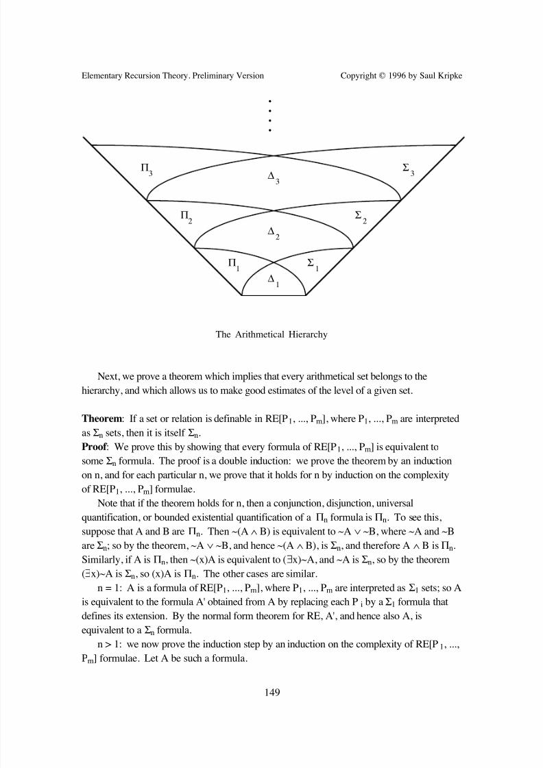
7/28/2019 Kripke Recursion Theory
http://slidepdf.com/reader/full/kripke-recursion-theory 153/191
Elementary Recursion Theory. Preliminary Version Copyright © 1996 by Saul Kripke
149
∆1
∆2
∆3
Π1
Π2
Π3
Σ1
Σ3
•
•
•
•
Σ2
The Arithmetical Hierarchy
Next, we prove a theorem which implies that every arithmetical set belongs to the
hierarchy, and which allows us to make good estimates of the level of a given set.
Theorem: If a set or relation is definable in RE[P1, ..., Pm], where P1, ..., Pm are interpreted
as Σn sets, then it is itself Σn.
Proof : We prove this by showing that every formula of RE[P1, ..., Pm] is equivalent to
some Σn formula. The proof is a double induction: we prove the theorem by an induction
on n, and for each particular n, we prove that it holds for n by induction on the complexity
of RE[P1, ..., Pm] formulae.
Note that if the theorem holds for n, then a conjunction, disjunction, universal
quantification, or bounded existential quantification of a Πn formula is Πn. To see this,
suppose that A and B are Πn. Then ~(A ∧ B) is equivalent to ~A ∨ ~B, where ~A and ~B
are Σn; so by the theorem, ~A ∨ ~B, and hence ~(A ∧ B), is Σn, and therefore A ∧ B is Πn.
Similarly, if A is Πn, then ~(x)A is equivalent to (∃x)~A, and ~A is Σn, so by the theorem
(∃x)~A is Σn, so (x)A is Πn. The other cases are similar.
n = 1: A is a formula of RE[P1, ..., Pm], where P1, ..., Pm are interpreted as Σ1 sets; so A
is equivalent to the formula A' obtained from A by replacing each P i by a Σ1 formula that
defines its extension. By the normal form theorem for RE, A', and hence also A, is
equivalent to a Σn formula.
n > 1: we now prove the induction step by an induction on the complexity of RE[P1, ...,
Pm] formulae. Let A be such a formula.
7/28/2019 Kripke Recursion Theory
http://slidepdf.com/reader/full/kripke-recursion-theory 154/191
Elementary Recursion Theory. Preliminary Version Copyright © 1996 by Saul Kripke
150
A is atomic: then either A is an atomic formula of RE or a formula Pi(x); in either case,
A is equivalent to a Σn formula.
A = B ∧ C: then B and C are equivalent to Σn formulae (∃y1)B' and (∃y2)C', so A isequivalent to (∃y1)(∃y2)(B' ∧ C'). This in turn is equivalent to (∃y)(∃y1 < y)(∃y2 < y)(B' ∧C'). Now since B' and C' are Πn-1, it follows (by the inductive hypothesis on n and the
remarks at the beginning of the proof) that (∃y1 < y)(∃y2 < y)(B' ∧ C') is also Πn-1. That is,
(∃y1 < y)(∃y2 < y)(B' ∧ C') is equivalent to some Πn-1 formula D, so (∃y)(∃y1 < y)(∃y2 <
y)(B' ∧ C'), and hence A, is equivalent to the Σn formula (∃y)D.
A = B ∨ C: B and C are equivalent to Σn formulae (∃y)B' and (∃y)C', where B' and C'
are Πn-1; so A is equivalent to (∃y)(B' ∨ C'), and again B' ∨ C' is Πn-1, so A is Σn.
A = (∃y)B. Then B is equivalent to a Σn formula (∃z)B', so A is equivalent to
(∃y)(∃z)B', where B' is a Πn-1 formula; this in turn is equivalent to (∃w)(∃y < w)(∃z < w)B',
and again (∃y < w)(∃z < w)B' is Πn-1, so the whole formula is Σn.
A = (x < t)B: then A is equivalent to (x < t)(∃y)B' for some Πn-1 formula B', which is in
turn equivalent to (∃w)(x < t)(∃y < w)B'; again, (x < t)(∃y < w)B' is Πn-1, so the whole
formula is Σn.
Notice that the proof is really just an elaboration of the proof of the normal form theorem
for RE.
We now have:
Theorem: All arithmetical sets and relations are Σn for some n.Proof: We show, by induction on the complexity of formulae of the language of arithmetic,
that those formulae define relations that are Σn for some n. Atomic formulae define Σ1 sets.
Suppose A defines a Σm relation and B defines a Σp relation. Letting n = max(m, p), A and
B both define Σn relations. A ∧ B, A ∨ B, and (∃y)A define Σn relations, as we have seen.
~A defines a Πn relation, which is also a Σn+1 relation. Finally, (y)A defines a Πn+1
relation, which is also a Σn+2 relation.
We could have proved this more quickly. We could, for example, have used Kleene's
proof: to show that a formula A of the language of arithmetic is equivalent to a Σn formula,
put A into prenex normal form, and then contract blocks of like quantifiers (i.e. allexistential or all universal) into a single quantifier. (The contraction could use the pairing
function, or it could imitate the above proof.) More quickly still, to obtain a Σn formula
equivalent to A, put A into prenex normal form and then add enough vacuous quantifiers to
make the unbounded quantifiers alternate.
The virtue of the above theorem is that it gives us a way of calculating a good estimate of
the level of arithmetical sets and relations. If A is a formula of the language of arithmetic,
first move all negation signs in (either all the way in, or far enough in that they only occur
before formulae whose levels are known). The resulting formula will be built up via
7/28/2019 Kripke Recursion Theory
http://slidepdf.com/reader/full/kripke-recursion-theory 155/191
Elementary Recursion Theory. Preliminary Version Copyright © 1996 by Saul Kripke
151
conjunction, disjunction, and existential and universal quantification from formulae whose
levels are known. We can then use the theorem to get an estimate of the level of the
formula, using e.g. the facts that (∃x)B is Σn if B is and that if B and C are Σm and Σp,respectively, then A ∧ B and A ∨ B are Σn, where n = max(m, p). Alternatively, if all of the
unbounded quantifiers occur at the beginning of the formula, we can use the theorem to
contract blocks of like quantifiers and read an estimate of the formula's level directly off the
result.
Suppose the predicates P1, ..., Pm in the theorem all define Πn sets. In that case, they
define Σn+1 sets, so every set or relation definable in RE[P1, ..., Pm] is Σn+1. Since being
definable in RE[P1, ..., Pm] is the same as being enumeration reducible to S1, ..., Sm, it
follows that any set or relation enumeration reducible to a Πn set is Σn+1. In fact, the
converse is true: any Σn+1 set is ≤e some Πn set. To see this, let S be any Σn+1 set, and let
(∃z)A(x, z) be a Σn+1 formula that defines it. Then A(x, z) defines a Πn relation R, so S ≤e
R (since S is defined by the formula (∃z)P21(x, z) of RE[P2
1]), and therefore S ≤e {[x, y]:
R(x, y)}, which is easily seen to be Πn. So a set or relation is Σn+1 iff it is ≤e some Πn set.
Thus, we begin to see a relation between the arithmetical hierarchy and the various
reducibility notions. We shall examine this relation further, and prove a famous theorem of
Post relating the arithmetical hierarchy to the jump hierarchy (i.e. the hierarchy 0, 0', 0'',...).
Exercises
1. Calculate upper bounds as good as you can find for the levels in the arithmetical
hierarchy of the following sets:
{e: We is infinite};
{e: We is recursive};
{e: We is nonempty};
{e: Φe is a total function}.
2. (a) In the class we defined a set S as total (with respect to enumeration reducibility) iff
-S≤eS. (i) Prove that if S is any set, S U -S is always total. (ii) Prove also that a set Sconsisting of ordered pairs [m,n] that codes the graph of a total function (not necessarily
recursive) is total. (iii) Which r.e. sets are total? (iv) If S is any set, and S+ is the set of pairs
coding the graph of the characteristic function of S, prove that S+≡eS U -S. (v) Prove the
following normal form theorem, whenever the predicate P11 is interpreted by a set S coding
the graph of a total function: every enumeration operator when confined to such sets can be
written in the form (∃s)(R(x,s) ∧ s⊆P11 ∧ (j≤s)(n≤s)([j,n]∈s ⊃ (i<j)(∃m≤s)([i,m]∈s)))
where R is an r.e. relation. (Given that S codes the graph of a total function, the clauses at
the end mean that s codes a partial function whose domain is a finite initial segment of the
7/28/2019 Kripke Recursion Theory
http://slidepdf.com/reader/full/kripke-recursion-theory 156/191
Elementary Recursion Theory. Preliminary Version Copyright © 1996 by Saul Kripke
152
natural numbers.)
(b) An enumeration degree is called total if it contains at least one total set. (i) Prove that
an enumeration degree is total iff it contains a set of pairs that codes the graph of some totalfunction. (ii) Prove that the Turing degrees, as a partially ordered structure, are isomorphic
to the total enumeration degrees. (iii) Prove that every enumeration degree contains a set
coding the graph of a partial function. (For this reason, enumeration degrees are sometimes
called partial degrees.) (iv) Give an example of a set that is not total but whose enumeration
degree is nevertheless total. (v) Show that if S is any fixed-point of the function φ defined in
exercise 5 of Lecture XVIII, then the enumeration degree of S is not total.
3. Here is yet another variation on the notion of a 1-complete set. A set S is said to be
"weakly creative" iff S is r.e. and there is a partial recursive function φ such that whenever
Wx ∩ S = Ø, φ(x) is defined and φ(x) ∉ S ∪ Wx. The difference between the notions
"weakly creative" and creative is that here φ need not be total. (We can call φ a "weakly
creative" function for S.) Actually, this definition was the original definition of "creative".
Prove that all weakly creative sets are creative. (Hint: show that for every partial recursive
function φ there is a total recursive χ such that Wχ(x) = Wx if φ(x) is defined, Wχ(x) = Ø
otherwise. Define ψ (x) = φ(χ(x)). Show that ψ is total recursive and is a creative function
for S if φ is a weakly creative function for S.)
This will complete our list of equivalent notions: weakly creative, creative, 1-1 creative,
completely creative, 1-1 completely creative, many-one complete, 1-1 complete, and satisfies
the effective form of Gödel's theorem. There are a few others, but we'll stop here.
7/28/2019 Kripke Recursion Theory
http://slidepdf.com/reader/full/kripke-recursion-theory 157/191
Elementary Recursion Theory. Preliminary Version Copyright © 1996 by Saul Kripke
153
Lecture XXI
The Arithmetical Hierarchy and the Jump Hierarchy.
Let us now look at some of the interrelations between the notions Σn and Πn on the one
hand, and the notions connected with relative recursiveness on the other. We proved that a
set is Σn+1 iff it is enumeration reducible to some Πn set. If S is enumeration reducible to a
Πn set, then a fortiori it is r.e. in a Πn set, or equivalently, in a Σn set. (S1 is r.e. in S2 iff S1
is r.e. in -S2, by the definition of "r.e. in".) Now suppose S1 is r.e. in a Πn set S2. Then S1
is definable in RE[P1, P2], with P1 and P2 interpreted as S2 and -S2, respectively. Both S2
and -S2 are Σn+1, so S1 is itself Σn+1. Thus we have the following result.
Theorem: A set S is Σn+1 iff S is enumeration reducible to a Πn set, iff S is r.e. in a Πn set,
iff S is r.e. in a Σn set.
Let us now relate this to the hierarchy 0, 0', 0'', ... of degrees. We first prove the following
Lemma: For all n, a set is r.e. in Ø(n) iff it is Σn+1.
Proof : We prove this by induction on n. For n = 0, the theorem states that a set is Σ1 iff it
is r.e. in Ø. But a set is r.e. in Ø iff it is r.e., so the theorem states that a set is r.e. iff it is Σ1,which we already know to be the case.
Now let n > 0, and suppose the theorem holds for everything less than n.
⇒: Suppose S is r.e. in Ø(n). By the properties of the jump operator, Ø(n) = Ø(n-1)' is
r.e. in Ø(n-1). By the inductive hypothesis, then, Ø(n) is Σn. So S is r.e. in a Σn set and is
therefore Σn+1.
⇐: Suppose S is Σn+1. Then S is r.e. in some Σn set S1. By the inductive hypothesis,
S1 is r.e. in Ø(n-1). By the jump properties, S1 ≤1 Ø(n-1)' = Ø(n), so a fortiori S1 ≤T Ø(n).
By the weak transitivity property of r.e. in, S is r.e. in Ø(n).
If d is a Turing degree, we can say that a set S is r.e. in d iff S is r.e. in some set in d. If S is r.e. in a given set in d, then S is r.e. in every set in d: suppose S is r.e. in S1 ∈ d, and
S2 ∈ d; then S1 ≤T S2, so by the weak transitivity property, S is r.e. in S2. By the same
reasoning (this time using the transitivity of ≤T), we can say that a set is recursive in d iff it
is recursive in some, or equivalently every, set in d. Thus we can restate the above result as
follows:
Corollary: A set is Σn+1 iff it is r.e. in 0(n).
Proof : 0(n) is the degree of Ø(n).
7/28/2019 Kripke Recursion Theory
http://slidepdf.com/reader/full/kripke-recursion-theory 158/191
Elementary Recursion Theory. Preliminary Version Copyright © 1996 by Saul Kripke
154
We also have the following:
Corollary (Post's Theorem): A set is recursive in 0(n) iff it is ∆n+1.
Proof : S is recursive in 0(n) iff both S and -S are r.e. in 0(n), iff both S and -S are Σn+1, iff
S is ∆n+1.
This theorem was proved in a paper by Post in the early 40's; he also introduced the notions
of simple and creative sets in that paper. The paper, by the way, was very important
methodologically, as it was the first to rely heavily on the intuitive notion of a computation:
previous work in recursion theory was all written out in a very formal way.
Post's theorem might be more of a surprise given other formalisms than our own (e.g.
the Turing machine formalism), as it displays an intimate connection between the recursion-
theoretic jump hierarchy on the one hand and on the other the arithmetical hierarchy, which
was defined in terms of definability in a certain language.
* Given our own formalism this should be less surprising, since on our approach recursion-
theoretic notions are themselves given in terms of definability, and Post's theorem simply
shows that two different notions given in terms of definability match up in a certain way.
A set is said to be 1-complete Σ n (or simply complete Σ n) if it is a Σn set to which all Σn
sets are 1-1 reducible. Thus, a set is 1-complete Σ1 just in case it is 1-complete. We could
define m-complete Σ n analogously, but it turns out that, just as in the special case n = 1, the
two notions coincide.Before going on, we should notice that every set many-one reducible to a Σn set is itself
Σn. (So in particular, every set 1-1 reducible to a Σn set is Σn.) To see this, suppose S1 ≤m
S2 and S2 is Σn. Then there is a recursive function ψ such that S1 = {x: ψ (x) ∈ S2}, so S1
is defined by the formula (∃y)(PS(x, y) ∧ A(y)), where A is a Σn formula that defines S and
PS(x, y) is a Σ1 formula that defines the graph of ψ . We can then calculate the whole
formula to be Σn. (A(y) and PS(x, y) are both Σn, so their conjunction is, too; and adding an
existential quantifier to a Σn formula just yields another Σn formula.) Therefore, the set S1
is Σn.
It is immediate from this that any set many-one reducible to a Πn set is itself Πn. For
suppose S1 ≤m S2 and S2 is Πn; then -S1 ≤m -S2 and -S2 is Σn, so -S1 is Σn, and so S1 isΠn. If S many-one reduces to a ∆n set, then S many-one reduces to a set that is both Σn and
Πn, and is therefore itself both Σn and Πn, i.e. it is ∆n.
We can therefore show that A set S is complete Σn just in case for all S1, S1 is Σn ⇔ S1
≤1 S. Clearly, if S1 is Σn ⇔ S1 ≤1 S for all S1, then S is Σn (since S ≤1 S) and every Σn set
1-1 reduces to S, i.e. S is complete Σn. If, on the other hand, S is complete Σn, then S1 is Σn
⇒ S1 ≤1 S for all S1, so we only have to show that S1 ≤1 S ⇒ S1 is Σn. But we know that
S is Σn, so by the preceding remarks we know that any set 1-1 reducible to S is also Σn.
As a corollary to the lemma, we can deduce that each Ø(n) is complete Σn.
7/28/2019 Kripke Recursion Theory
http://slidepdf.com/reader/full/kripke-recursion-theory 159/191
Elementary Recursion Theory. Preliminary Version Copyright © 1996 by Saul Kripke
155
Theorem: For all n > 0, Ø(n) is complete Σn.
Proof : This is just to say that for all S, S ≤1 Ø(n) iff S is Σn. But S ≤1 Ø(n) iff S is r.e. inØ(n-1), by the jump properties, iff S is Σn, by the lemma.
We therefore have several different characterizations of th
e Σn+1 sets:
S is Σn+1 ⇔ S ≤e some Πn set ⇔ S is r.e. in some Σn set
⇔ S is r.e. in Ø(n) ⇔ S ≤1 Ø(n+1) ⇔ S ≤m Ø(n+1).
(As for the last biconditional: if S ≤1 Ø(n+1) then obviously S ≤m Ø(n+1), and if S ≤m Ø(n+1)
then, since Ø(n+1) is Σn+1, S is also Σn+1.)
Trial-and-Error Predicates.
In the special case n = 1, Post's theorem implies that the ∆2 sets are precisely the sets
recursive in 0'. There are also other interesting characterizations of the ∆2 sets.
One such characterization has to do with a modification of the notion of a computation.
Consider a computing machine that gives tentative answers to questions that are put to it.
When asked "is x in S?", it may answer "yes", but then later on change its mind and answer"no". In fact, it may change its mind several times; however, we require it to settle on a
single answer after a finite number of changes of mind. If M is such a machine, the set
computed by M is the set {x: M eventually settles on a "yes" answer for the input x}.
Once this notion is made precise, it turns out that the sets computed by such machines are
precisely the ∆2 sets. (The notion of this kind of computation, and this result, are due to
Hilary Putnam.)
One way to make this precise is as follows. Consider a total recursive function ψ in two
variables which takes only the values 0 and 1. Suppose that for any m, there is an s0 such
that ψ (m, s) = ψ (m, s0) for all s ≥ s0. (s0 need not be the same for all m.) ψ represents a
machine of the sort we are considering, and ψ (m, s) represents the sth answer given for theinput m. (0 and 1 represent the answers "no" and "yes", respectively.) The set associated
with the function ψ is the set S = {m: ψ (m, s0) = 1, where ψ (m, s0) = ψ (m, s) for all s ≥ s0}.
(Since s0 depends on m, we can equivalently define S = {m: ψ (m, ρ(m)) = 1}, where ρ is
any function such that for all m and for all s ≥ ρ(m), ψ (m, s) = ψ (m, ρ(m)). ρ(m) need not
be the least such s0. ρ is called a modulus of convergence for ψ . S will always be recursive
in any modulus of convergence for ψ .)Let us call a set associated with such a ψ in the indicated way a trial-and-error
predicate. It can be shown that the trial-and-error predicates are precisely the ∆2 sets. The
7/28/2019 Kripke Recursion Theory
http://slidepdf.com/reader/full/kripke-recursion-theory 160/191
Elementary Recursion Theory. Preliminary Version Copyright © 1996 by Saul Kripke
156
proof that all trial-and-error predicates are ∆2 is easy and is left as an exercise for the reader.
The other direction is harder, and we shall sketch an informal proof. First, notice that any
r.e. set is a trial-and-error predicate, for suppose S is r.e. and let P be any semi-computationfor S. Then we can compute S (in the present sense of "compute") by setting P going and
giving "no, no, no, ..." as output. If and when P says "yes", then we change our minds and
start giving "yes, yes, ..." as output; if at any point P has not said anything, however, we
continue to say "no". Thus, our outputs involve only a finite number of changes of mind
(either one or none at all), so we have computed S in the appropriate sense. So all Σ1 sets
are trial-and-error predicates; the same applies to Π1 sets by reversing "yes" and "no".
Now consider the general case. Suppose a set S is ∆2; then it is recursive in some
particular r.e. set (Ø', for example). So S is computed by some procedure P with an oracle
to Ø'. Since Ø' is r.e., we have a trial-and-error machine for Ø'. For a given x, we can
compute tentative answers to the question "is x in S?" as follows. Suppose we are being
asked for the nth time. We run P for n steps, except that when P consults its oracle about
whether a ∈ Ø', we ask our trial-and-error machine whether a ∈ Ø'. (If n > 1, then we may
have asked it this question before.) If after n steps we have obtained an answer, we give that
answer; otherwise we say "no" (or "yes"; it doesn't matter which). Now, when P is run with
an oracle to Ø', the oracle is consulted only finitely many times before P halts with the
correct answer to whether x ∈ S, i.e. there is a finite collection a1, ..., ak of sets such that
when P is given correct answers to the questions "a1 ∈ Ø'?", ..., "ak ∈ Ø'?", and is given
enough time to run, it will halt with the correct answer to the question "x ∈ S?". So we will
eventually reach a stage in our computation such that we have asked the trial and errormachine the questions "a1 ∈ Ø'?", ..., "ak ∈ Ø'?" often enough to get correct answers, and
such that we run P long enough to get an answer, which must be the correct answer, to
whether x ∈ S. So for any x, there is an n large enough that our computation always gives
the correct answer to "x ∈ S?" after stage n.
The Relativization Principle.
There is a general principle in recursion theory, which is hard to make precise but which
ought to be stated nonetheless. It is that whenever we have a proof of some statement aboutthe absolute notion of recursiveness or recursive enumerability, then we can demonstrate,
using essentially the same proof, an analogous statement about the relative notion of
recursiveness in a set or of recursive enumerability in a set. Or in general, any statement
involving an absolute notion relativizes to the corresponding relative notion and by the same
proof, provided the relative notion involves an oracle (or extra predicate, etc.) to both a set
and its complement. This must be taken with a grain of salt, since if we have shown that
some particular set is not recursive, or that it is not r.e., we do not thereby show that there is
no set in which it is recursive or r.e. However, this is not the sort of statement that is
7/28/2019 Kripke Recursion Theory
http://slidepdf.com/reader/full/kripke-recursion-theory 161/191
Elementary Recursion Theory. Preliminary Version Copyright © 1996 by Saul Kripke
157
intended in the principle; once one has some experience with this principle, one gets a feel
for what sort of statements are and are not allowed.
Consider, for example, the result that K is r.e. but not recursive. Let us define, for anygiven set S, WS to be the relation {<e, m>: (∃s)(s ⊆ S U -S ∧ W(e, x, s))}. WS is thus an
enumeration of the sets r.e. in S. Thus, for any e, WSe is the set {m: (∃s)(s ⊆ S U -S ∧
W(e, x, s))}, and S' is simply the set {[e, m]: m ∈ WSe}. We can define KS to be the set {e:
e ∈ WSe}. KS really has the same definition as K, except that we now relativize the relevant
notions to S. The analog of the fact that K is r.e. but not recursive is the fact that KS is r.e.
in S but not recursive in S; this holds, and is shown by the very same proof we used to
show that K is r.e. but not recursive.
As another example, we can relativize the Σn-Πn hierarchy to a set S by considering
formulae in the language of arithmetic plus an extra predicate interpreted as S. (We thereby
get an atomic formula, namely ~P(x), which defines the complement of S, since the
language of arithmetic has negation.) Thus, we have the relativized notions Σ n in S andΠ nin S , with the obvious definitions. We similarly say that a set or relation is arithmetical in S
if it is defined by some formula in the language of arithmetic with the extra predicate
interpreted as S. We can prove, by the same proofs we used to prove the corresponding
absolute theorems, that every set arithmetical in S is either Σn or Πn in S for some n, that
there is an enumeration of the sets Σn (or Πn) in S which is itself Σn (Πn) in S, and that
there is always a set that is Πn in S but not Σn in S. We also have a relativized version of
Post's theorem, and by the same proof: if d is the degree of S, then a set is ∆n+1 in S iff it is
recursive in d(n)
.Now, people have tried to state the relativization principle formally, but every attempt so
far has been unsuccessful. That is, every formal claim which has been put forth as a
candidate statement of the principle has turned out to have counterexamples; however, these
counterexamples are not intuitively counterexamples to the relativization principle itself.
The relativization principle does not hold for complexity theory. Whereas in recursion
theory we do not place a time limit on a computation procedure, complexity theory is
concerned with computations for which a time limit is given in advance. Corresponding to
the question whether every r.e. set is recursive is the complexity-theoretic problem whether
P = NP, which is unsolved to this day. Whatever the answer may be to this problem,
however, we can be sure that it provides a counterexample to the relativization principle. Wecan relativize the P = NP problem by considering computations with an oracle to a given set;
it turns out that there are some oracles for which P = NP and some for which P ≠ NP.
Obviously, if a relativization principle held in complexity theory, then we would have either
P = NP for all oracles or P ≠ NP for all oracles.
7/28/2019 Kripke Recursion Theory
http://slidepdf.com/reader/full/kripke-recursion-theory 162/191
7/28/2019 Kripke Recursion Theory
http://slidepdf.com/reader/full/kripke-recursion-theory 163/191
Elementary Recursion Theory. Preliminary Version Copyright © 1996 by Saul Kripke
159
ψ (m) is the Gödel number of a Σn sentence equivalent to ~B, and let PS(x, y) be a Σ1
formula that defines the graph of ψ . Then a Πn sentence B is true iff ~B is not true, so
(y)(PS(x, y) ⊃ ~A(y)) defines truth for Πn sentences, and is equivalent to a Πn formula.Now we know already that there is a Σ1 formula that defines truth for Σ1 sentences, so
the theorem holds for n = 1. Suppose it holds for n, and let A(x) be a Πn formula that
defines truth for Πn sentences. Let χ be a recursive function such that if (∃x)C(x) is a Σn+1
sentence with Gödel number m, then χ(m, p) is the Gödel number of C(0(p)), and let CH(x,
y) be a Σ1 formula that defines the graph of χ. (∃x)C(x) is true iff for some C(0(p)) is true
for some p, so (∃y)(∃z)(CH(x, z, y) ∧ A(y)) defines truth for Σn+1 sentences and is itself
Σn+1. As we have already seen, it follows that there is a Πn+1 formula that defines truth for
Πn+1 sentences, so we are done.
7/28/2019 Kripke Recursion Theory
http://slidepdf.com/reader/full/kripke-recursion-theory 164/191
Elementary Recursion Theory. Preliminary Version Copyright © 1996 by Saul Kripke
160
Lecture XXII
Theω -rule.
Recall that Gödel's theorem gives us a universally quantified statement (x)A(x) all of whose
instances are provable but which is not itself provable. Thus, while intuitively it might seem
like (x)A(x) follows from A(0), A(0'), ..., in fact, while all of the latter are provable, the
former is not provable. However, it would be provable if we added to our formal system the
following rule, known as the ω -rule: from A(0), A(0'), ... to infer (x)A(x). In fact, this was
Hilbert's suggestion when he first heard about Gödel's result.
Theω -rule can't actually be applied in practice, since it has infinitely many premises and
so a proof using the ω -rule would be infinitely long. Moreover, even if we can prove each
of the instances of (x)A(x), we may not be in a position to know that they are all provable.
For example, consider Goldbach's conjecture. Supposing that it is in fact true, we can easily
prove each of its instances; nonetheless, we are not now in a position to know that all of its
instances are provable, since we are not now in a position to prove that the statement itself is
true.
Nonetheless, we can consider formal systems which contain the ω -rule, even if we
cannot actually use such systems. If we add theω -rule to an ordinary first-order deductive
system (Q, for example), then not only will there be no true but unprovable Π1 statements:
all true statements will be provable. To see this, suppose we start out with a system whichproves all true sentences of Lim, and which is such that every sentence of the language of
arithmetic is provably equivalent to a Σn orΠn sentence, for some n. If we add theω -rule to
such a system, then we will be able to prove every true Σn orΠn sentence, and therefore
every true sentence whatsoever. We show this by induction on n. (For the sake of the
proof, we define a formula to be both Σ0 andΠ0 if it is a formula of Lim.) We know it
holds for n = 0, because by hypothesis all true sentences of Lim are provable. Suppose it
holds for n, and let A be a Σn+1 formula. Then A is (∃x)B(x) for some Πn formula B(x). If
A is true, then B(0(m)) is true for some m, so by the inductive hypothesis B(0(m)) is
provable in the system, so A is also provable. Now let A be a Πn+1 formula. Then A is
(x)B(x) for some Σn formula B(x). If A is true, then B(0(m)) is true for all m, so by theinductive hypothesis, B(0(m)) is provable for all m. Now we apply theω -rule: from the
sentences B(0), B(0'), ..., we can infer the sentence (x)B(x), i.e. the sentence A, so A is
provable.
So as long as we stay within the first-order language of arithmetic, we can get around
the Gödel theorem by allowing our formal systems to include the ω -rule. However, if we
consider richer languages (e.g. languages with quantifiers over sets of numbers, or with
extra predicates), we will not necessarily be able to get around the Gödel result in this way.
In fact, there are languages richer than the first-order language of arithmetic such that, even
7/28/2019 Kripke Recursion Theory
http://slidepdf.com/reader/full/kripke-recursion-theory 165/191
7/28/2019 Kripke Recursion Theory
http://slidepdf.com/reader/full/kripke-recursion-theory 166/191
Elementary Recursion Theory. Preliminary Version Copyright © 1996 by Saul Kripke
162
universal. Thus, for example, the formula (α)(∃β)(x) α(x) = β(x) is a Π12 formula. A
relation is Σ1n or Π1
n if it is defined by a Σ1n or Π1
n formula, respectively; a relation is ∆1n if it is
both Σ1n and Π
1n. The hierarchy of Σ
1n and Π
1n sets is called the analytical hierarchy. This
hierarchy was first studied by Kleene, who invented its name.
In general, a Σmn or Πm
n formula is an alternating string of type-m quantifiers of length n
followed by a formula containing only quantifiers of type < m. Quantifiers over numbers
are type-0, quantifiers over functions on N, sets of numbers, etc., are of type 1, quantifiers
over sets of sets of numbers are of type 2, etc.
The analytical relations are not to be confused with the analytic relations, i.e. the Σ11
relations. When Kleene first studied the analytical hierarchy, a certain class of functions
had already been studied and were called "analytic"; it was only discovered later that these
functions are precisely the Σ11 functions. To avoid conflicting notations, the term
"analytical" was chosen for the more inclusive class. Nowadays, in order to avoid
confusion, the term "Σ11" is generally used instead of "analytic".
Normal Form Theorems.
An arithmetical formula is a formula that does not contain any quantifiers over functions
(though it may contain free function variables). We would like to show that every formula
is equivalent to some Σ1n or Π1
n formula (for some n), and in particular that every arithmetical
formula is equivalent to some Σ1
1 formula and to some Π1
1 formula. At this point it shouldbe far from obvious that this is the case, since a formula can have several number
quantifiers, and a Σ1n or Π1
n formula is only allowed to have a single number quantifier, and
that of the opposite type from the last function quantifier. In this section we shall show how
to find a Σ1n or Π1
n equivalent for any formula of the language of arithmetic.
Clearly, any formula can be put into prenex form. (We consider a formula to be in
prenex form if it consists of a string of unbounded quantifiers followed by a formula of
Lim.) However, the initial string of quantifiers that results may not alternate, and it may also
include number quantifiers. So to put the formula in the desired form, we must move the
number quantifiers to the end of the string, collapse them to a single quantifier of the
opposite type from the last function quantifier, and make the string of function quantifiersalternate.
First, let us work on moving the number quantifiers to the end. To do this, it suffices to
show that any formula of the form (Qx)(Q'α)A is equivalent to a formula (Q'α)(Qx)A*,
where Q and Q' are quantifiers and A differs from A* only in the part that is in Lim: if we
have this result, then we can apply it repeatedly to any prenex formula to produce an
equivalent prenex formula with all the number quantifiers at the end. This is easy to show
when Q = Q': (∃x)(∃α)A is always equivalent to (∃α)(∃x)A, and (x)(α)A is always
equivalent to (α)(x)A. So the only difficult case is when Q ≠ Q'.
7/28/2019 Kripke Recursion Theory
http://slidepdf.com/reader/full/kripke-recursion-theory 167/191
Elementary Recursion Theory. Preliminary Version Copyright © 1996 by Saul Kripke
163
Consider a formula of the form (x)(∃α)A. This is true just in case for every number x
there is a function αx such that A(x, αx) holds. Letting Φ(x) = αx, this implies that there is
a function Φ such that for all x, A(x, Φ(x)) holds; conversely, if such an Φ exists, thenobviously (x)(∃α)A(x, α) holds. Φ is a higher-order function, and the quantifiers in our
formulae only range over functions from N to N, so we cannot rewrite (x)(∃α)A as
(∃Φ)(x)A(x,Φ(x)). However, there is a way to get around this. SupposeΦ maps numbers
onto functions; then let γ be the function from N to N such that γ ([x, y]) = (Φ(x))(y). Let
A*(x, γ ) be the result of replacing all occurrences of α(t) in A by γ ([x, t]), for any term t;
clearly, A and A* differ only in the part that is in Lim. It is easy to see that A*(x, γ ) holds
iff A(x, Φ(x)) holds. Therefore, (x)(∃α)A holds iff there is a Φ such that for all x, A(x,
Φ(x)) holds, iff there is a γ such that for all x, A*(x, γ ) holds, iff (γ )(∃x)A*(x, γ ) holds. So
we have the desired result in this case.
There is only one remaining case, namely the case of formulae of the form (∃x)(α)A(x,
α). But (∃x)(α)A(x, α) is equivalent to ~(x)(∃α)~A(x, α), which, as we have just seen, is
equivalent to ~(∃γ )(x)~A*(x, g), which is equivalent to (γ )(∃x)A*(x, γ ). So we have proved
the following
Theorem: Any formula is equivalent to a prenex formula in which all the unbounded
number quantifiers occur at the end.
Notice that, in moving from (x)(∃α)A to (∃Φ)(x)A(x, Φ(x)), we have assumed the axiom of
choice: if the axiom of choice fails, then even though for every x there is anα such thatA(x, α) holds, there may be no single function which takes x to an appropriate α.
The initial string of function quantifiers may not yet alternate. However, using the
pairing function, we can collapse adjacent quantifiers of the same type into a single
quantifier, and by repeating this process, we can make the initial string alternate. That is, for
any formula A(α, β), let A*(γ ) be a formula that differs from A only in the Lim part, and
such that A(α, β) is equivalent to A*([α, β]) for all α, β. (Such an A* is easy to find.)
Then (∃α)(∃β)A(α, β) is equivalent to (∃γ )A*(γ ), and (α)(β)A(α, β) is equivalent to
(γ )A*(γ ). (Here we are assuming that our pairing function is onto.) Thus, we have the
following
Theorem: Any formula is equivalent to a prenex formula consisting of an alternating string
of function quantifiers followed by a first-order formula.
To get the desired result, we must show how to collapse the number quantifiers into a
single quantifier. We shall do this by proving that any first-order formula is equivalent to
both a Σ11 and a Π1
1 formula. Once we have done this, we can prove our main result as
follows. Let A be any formula, and take any prenex equivalent with all the function
quantifiers in front. Suppose the last function quantifier is existential, and let B be the first-
7/28/2019 Kripke Recursion Theory
http://slidepdf.com/reader/full/kripke-recursion-theory 168/191
Elementary Recursion Theory. Preliminary Version Copyright © 1996 by Saul Kripke
164
order part of the formula. Then A is equivalent to a formula (Qα1)...(∃αn)B. Now let
(∃αn+1)(x)C be a Σ11 equivalent of B; A is equivalent to (Qα1)...(∃αn) (∃αn+1)(x)C. We
can collapse the adjacent quantifiers (∃αn) and (∃αn+1); thus A is equivalent to(Qα1)...(∃αn)(x)D, with D in Lim, i.e. A is equivalent to a Σ1
n formula. If the last function
quantifier is universal we argue similarly, this time using a Π11 equivalent of B.
Theorem: Every first-order formula is equivalent to both a Σ11 and a Π1
1 formula.
Proof : Let A be any first-order formula. We know already that we can take A to be either
Σ0n or Π0
n, for some n. By adding vacuous quantifiers if necessary, we can assume that A is
Π0n for some n and that n is even. Thus, A is equivalent to a formula
(x1)(∃y1)...(xm)(∃ym)B with B in Lim. Now any formula (x)(∃y)C(x, y) is equivalent to
(∃α)(x)C(x, α(x)), as we can see using the same sort of argument we used before. (If
(∃α)(x)C(x, α(x)) holds, then obviously (x)(∃y)C(x, y) holds; conversely, if (x)(∃y)C(x, y)
holds, then (∃α)(x)C(x, α(x)) holds, letting α(x) = the least y such that C(x, y) holds.)
Iterating this, and moving the number quantifiers to the end, we see that A is equivalent to
(∃α1)...(∃αm)(x1)...(xm)B' for B' in Lim. We can collapse the existential function
quantifiers, and we can also collapse the universal number quantifiers using a bounding
trick. The result is Σ11, so A is equivalent to a Σ1
1 formula.
To see that A is also equivalent to a Π11 formula, notice that the foregoing argument
shows that the formula ~A is equivalent to some Σ11 formula (∃α)(x)B, and so A itself is
equivalent to the Π11 formula (α)(∃x)~B.
By the foregoing remarks, we finally have our main result.
Theorem: Every formula is equivalent to someΠ1n or Σ1
n formula, for some n. Moreover, if
A is a formula consisting of an alternating string of quantifiers of length n, the first
quantifier of which is existential (universal), followed by a first order formula, then A is
equivalent to a Σ1n (Π1
n) formula.
(The trick of replacing (x)(∃y)C(x, y) by (∃α)(x)C(x, α(x)) is due to Skolem. Notice
that, in contrast to the previous case, we have not assumed the axiom of choice, since we
definedα(x) to be the least y such that C(x, y). We were able to do this because we know
that our domain (viz. N) can be well-ordered. Skolem's trick can be applied to any domainthat can be well-ordered; however, if the axiom of choice fails, then there will be domains
that cannot be well-ordered.)
As with the arithmetical hierarchy, we can define the level of an analytical relation to be
the least inclusive Σ1n, Π1
n, or ∆1n of which it is an element. The above discussion gives us
ways of estimating the level of a given analytical relation.
All arithmetical relations are ∆11, as we have seen. Moreover, if A is a Σ1
n formula, then
(∃α)A is equivalent to a Σ1n formula since we can collapse (∃α) with A's initial quantifier;
similarly, if A is a Π1n formula, then (α)A is equivalent to a Π1
n formula. In short, the Σ1n and
7/28/2019 Kripke Recursion Theory
http://slidepdf.com/reader/full/kripke-recursion-theory 169/191
Elementary Recursion Theory. Preliminary Version Copyright © 1996 by Saul Kripke
165
Π1n relations are closed under existential and universal functional quantification, respectively.
Similarly, if A is Σ1n, then so are both (x)A and (∃x)A, and the same is true if A is Π1
n. This
is because, as we have seen, we can always move number quantifiers inwards withoutaffecting the variable quantifiers.
It is also not hard to see that if A and B are Σ1n (or Π1
n), then so are A ∧ B and A ∨ B.
We can show this by induction on n. Since Σ10 = Π1
0 = {arithmetical relations}, this clearly
holds for n = 0. Suppose it holds for n. If A and B are Σ1n+1, then they are (∃α)C and
(∃β)D for Π1n formula C and D. Then A ∧ B and A ∨ B are equivalent to (∃α)(∃β)(C ∧ D)
and (∃α)(∃β)(C ∨ D), respectively, which are Σ1n+1, by the inductive hypothesis and
collapsing the quantifiers (∃α) and (∃β). If A and B are Π1n+1, we argue similarly.
Thus, the situation is similar to that of the arithmetical hierarchy, except that function
quantifiers and unbounded number quantifiers play the role here that bounded and
unbounded number quantifiers play in the arithmetical case. Using a similar argument to
the one we gave there, we can see that if a relation is enumeration reducible to some Σ1n
(resp. Π1n) relations, then it is Σ1
n (resp. Π1n). It follows immediately that anything r.e. in a
∆1n relation is itself ∆1
n; a fortiori, anything recursive in a ∆1n relation is ∆1
n.
Exercise
1. Recall that A and B are recursively isomorphic (A ≡ B) iff there is a 1-1 total recursive
function φ whose range is N, and such that B = {φ(x): x ∈ A}. Show that for all A and B,A ≡ B iff A ≡1 B. The following sketches a method of proof. If A ≡ B, then A ≡1 B follows
easily, so suppose A ≡1 B. Let φ andψ be 1-1 recursive functions such that x ∈ A iff φ(x)
∈ B and x ∈ B iff ψ (x)∈A, all x. Define, a sequence a1, a2, ... and a sequence b1, b2, ..., as
follows. Suppose a1, ..., an and b1, ..., bn have been defined (where possibly n = 0). If n is
even, then let an+1 be the least number distinct from a1, ..., an, and let bn+1 be such that an+1
∈ A iff bn+1 ∈ B and bn+1 is distinct from all of b1, ..., bn. If n is odd, do the same thing in
reverse (i.e. let bn+1 be the least number distinct from b1, ..., bn, etc.). Moreover, do this in
such a way that the function χ such that χ(an) = bn for all n ∈ N is recursive. Conclude that
χ is a 1-1 total recursive function whose range is N, and such that for all x, x ∈ A iff χ(x)∈
B, and therefore that A ≡ B. Hint: Informally, the problem reduces to finding anappropriate bn+1 effectively from a1, ..., an, an+1 and b1, ..., bn (or an+1 from b1, ..., bn+1 and
a1, ..., an, if n is odd). If φ(an) ∉ {b1, ..., bn}, then we can put bn+1 = φ(an). However, we
may have φ(an) = bi for some i = 1, ..., n; show how to get around this.
A recursive isomorphism type is a ≡-equivalence class. Conclude that 1-degrees are
therefore recursive isomorphism types, and that there is a 1-degree (which is also an m-
degree and a recursive isomorphism type) which consists of the creative sets.
Comment: Dekker proposed that the notions studied by recursion theory should all be
invariant under recursive isomorphism. While all the notions studied in this course are
7/28/2019 Kripke Recursion Theory
http://slidepdf.com/reader/full/kripke-recursion-theory 170/191
Elementary Recursion Theory. Preliminary Version Copyright © 1996 by Saul Kripke
166
invariant under recursive isomorphism, there is at least one notion, that of a retraceable set,
which is not so invariant and which has been studied by recursion theorists. (Offhand, I
don't know whether this notion was proved to be not recursively invariant before Dekker'sproposal or only afterwards.)
7/28/2019 Kripke Recursion Theory
http://slidepdf.com/reader/full/kripke-recursion-theory 171/191

7/28/2019 Kripke Recursion Theory
http://slidepdf.com/reader/full/kripke-recursion-theory 172/191
Elementary Recursion Theory. Preliminary Version Copyright © 1996 by Saul Kripke
168
parameters.) This notion is not very interesting if R is a relation between numbers, since in
that case R will always be D01
(since R is always ∆01 in its characteristic function). However,
this is not the case if some of R's places are occupied by functions (i.e. if p > 0).Let's look at S0
1 in the case n = 0 and p = 1 (i.e. the case of S01 sets of functions). A set
S is S01 iff there is a 2-place Σ0
1 relation R and a function β such that S = {α: <α, β> ∈ R}.
We can also characterize the S01 sets topologically. Baire space is the topological space
whose points are total functions from N to N and whose open sets are those sets S such that
for every function φ in S, there is a finite initial segment s of φ such that every function
extending s is also in S. To verify that this is indeed a topological space, we must show that
if two sets satisfy our characterization of the open sets then their intersection does as well,
and that if F is a family of sets satisfying that characterization then∪F also satisfies it.
Alternatively, we can characterize Baire space as follows. For any finite sequence s, let Os =
{φ: φ is a total function which extends s}; then the sets of the form Os form a basis for
Baire space.
Theorem: The S01 sets are precisely the open sets of Baire space.
Proof : First, suppose S is S01. Then there is a 2-place Σ0
1 relation R between functions and
a particular function β such that S = {α: <α, β> ∈ R}. Suppose α ∈ S, i.e. <α, β> ∈ R.
By the monotonicity and finiteness properties of Σ01 relations, there is an initial segment s of
α such that <γ , β> ∈ R for all γ extending s, and therefore γ ∈ S for all such γ . Since α
was arbitrary, it follows that S is open.
Next, suppose S is open. Let F = {s: α ∈ S for all α extending s}. Then S = {α: αextends s for some s ∈ F}. Since F is a collection of finite sequences, we can let G = {n∈
N: n codes some element of F}, and let γ be G's characteristic function. Then S isΣ01 in γ ,
and therefore S01, since we can define S by the Σ0
1 formula (∃s)(γ (s) = 0' ∧ s ⊆ α). (Here s
⊆ α abbreviates the formula (n < s)(m < s)([n, m] ∈ s £ α(n) = m).)
Baire space is also homeomorphic to the irrational numbers under the usual topology. The
onto pairing function mentioned earlier is a homeomorphism between Baire space and its
direct product with itself; since Baire space is homeomorphic to the irrationals, this shows
that the irrational plane is homeomorphic to the irrational line. Thus, the situation is very
different from the case of the reals.We can set up a similar topology on sets of natural numbers by identifying these sets
with their characteristic functions; if we restrict Baire space to functions into {0, 1}, the
result is a space which is homeomorphic to the Cantor set. (That is, the set of all reals in the
interval [0, 1] whose base-3 expansions contain no 1's.) It is also identical to the space 2ω ,
where 2 is the space {0, 1} with the discrete topology.
Notice that since the S01 sets are precisely the open sets, the D0
1 sets are precisely the
clopen sets (i.e. sets that are both closed and open). This is another difference between the
reals and the rationals: whereas the only clopen subsets of R are R itself and Ø, clopen sets
7/28/2019 Kripke Recursion Theory
http://slidepdf.com/reader/full/kripke-recursion-theory 173/191
Elementary Recursion Theory. Preliminary Version Copyright © 1996 by Saul Kripke
169
of irrationals exist in great abundance.
Another Normal Form Theorem.
Given a function α, let us define α –(n) to be some numerical code for the sequence <α(0), ...,
α(n-1)>. It doesn't matter what particular code we choose; however, for definiteness, let us
say that α –(n) = 2α(0)+1.3α(1)+1.....pnα(n-1)+1, where in general pn is the nth prime. (This is
essentially the coding scheme Gödel used.) As Quine has remarked, coding systems are
not like matrimony, and we are free to switch back and forth between them as we please.
We now prove another normal form theorem, due to Kleene.
Theorem: If S is an n+p-place Σ01 relation, then there is an n+p-place recursive relation R
such that S = {<x1, ..., xn, α1, ..., αp>: (∃z)R(x1, ..., xn, α –1(z), ..., α –n(z))}.
Proof : We shall prove the theorem for the case n = 0 and p = 1; the other cases are similar.
Let S be a Σ01 set of functions. For some relation L(α, y) definable in Lim, S = {α:
(∃y)L(α, y)}. By monotonicity and finiteness, α ∈ S iff some initial segment of α is in S,
so S = {α: (∃z)(∃y)L(α –(z), y)}. In fact, S = {α: (∃z)(∃y < z)L(α –(z), y)}: if (∃z)(∃y <
z)L(α –(z), y) then certainly (∃z)(∃y)L(α –(z), y), and if L(α –(k), y), then let z > k, y; L(α –(z), y)
by monotonicity, so (∃z)(∃y < z)L(α –(z), y). Let R'(z, s) ≡ (∃y < z)L(s, z): R' is a recursive
relation, and S = {α: (∃z)R'(z, α –(z))}. This is almost what we want. Let R(s) ≡ R'(lh(s), s),
where lh(s) is the length of the sequence s; R is still recursive, and S = {α: (∃z)R(α –
(z))}.
This gives us a new normal form theorem forΠ11 relations.
Theorem: Every n+p-place Π11 relation is {<x1, ..., xn, α1, ..., αp>: (β)(∃z)R(x1, ..., xn, α –
)1(z), ..., α –p(z), β –
(z))} for some recursive relation R.
Proof : Let S be any n+p-place Π11 relation. Then S = {<x1, ..., xn, α1, ..., αp>: (β)T(x1, ...,
xn, α1, ..., αp, β)} for some n+p+1-place Σ01 relation T. By what we just proved, there is a
recursive relation R such that T(x1, ..., xn, α1, ..., αp, β) iff (∃z)R(x1, ..., xn, α –1(z), ..., α –p(z),
β –
(z)); it follows that S is {<x1, ..., xn, α1, ..., αp>: (β)(∃z)R(x1, ..., xn, α –1(z), ..., α –p(z), β –
)(z))}.
We can prove similar normal form theorems for the other Σ1n's and Π1
n's. The main thing to
note is that we have, so to speak, reduced the relation S, which may involve functions, to R, a
recursive relation among numbers.
There is a related result about the various S's and P's.
7/28/2019 Kripke Recursion Theory
http://slidepdf.com/reader/full/kripke-recursion-theory 174/191
Elementary Recursion Theory. Preliminary Version Copyright © 1996 by Saul Kripke
170
Theorem: An n+p-place relation S is S01 iff for some β and some recursive R, S = {<x1, ...,
xn, α1, ..., αp>: (∃z)R(x1, ..., xn, α –1(z), ..., α –p(z), β –
(z))}, iff for some n+p-place relation R
on N (not necessarily recursive), S = {<x1, ..., xn, α1, ..., αp>: (∃z)R(x1, ..., xn, α –1(z), ..., α –)p(z))}.
Proof : The equivalence of the first two conditions is immediate. Suppose S = {<x1, ..., xn,
α1, ..., αp>: (∃z)R(x1, ..., xn, α –1(z), ..., α –p(z), α –(z))}, and let R' be the relation {< x1, ..., xn, α –
)1(z), ..., α –p(z)>: z ∈ N and R(x1, ..., xn, α –1(z), ..., α –p(z), β –
(z))}; then S = {<x1, ..., xn, α1, ...,
αp>: (∃z)R'(x1, ..., xn, α –1(z), ..., α –p(z))}. Conversely, suppose S = {<x1, ..., xn, α1, ..., αp>:
(∃z)R(x1, ..., xn, α –1(z), ..., α –p(z))} for some relation R on N. Let β be the characteristic
function of the set {[x1, ..., xn, y1, ..., yp]: R(x1, ..., xn, y1, ..., yp)}. Then S = {<x1, ..., xn,
α1, ..., αp>: (∃z) β([x1, ..., xn, α –1(z), ..., α –p(z)]) = 1}, so S is Σ01 in β and is therefore S0
1.
Similar results hold for the other S's and P's.
The Hyperarithmetical Hierarchy.
Consider the hierarchy 0, 0', 0'', ..., 0(n), ... of degrees. As we have seen, a set is arithmetical
just in case it is recursive in one of these degrees. We also know that not all sets are
arithmetical (e.g. the set of true sentences of the language of arithmetic), so there are sets
which are not recursive in any of these degrees; therefore, there is a degree d which is not ≤
0(n) for any n. In fact, there are degrees d such that 0(n) < d for all n: it is not too hard tosee that the degree of the set of true sentences is such a degree. This suggests that we
should be able to extend the hierarchy 0, 0', 0'', ..., 0(n), ... into the transfinite in some way.
In particular, it suggests that there ought to be a natural next degree, which we can call
0(ω ), beyond all of the degrees 0(n). But what is 0(ω )? A natural answer would be that 0(ω ) is
the least upper bound of the degrees 0, 0', 0'', .... However, by a result due to Spector, that
collection of degrees does not have a least upper bound; so the most natural characterization
of 0(ω ) will not work.
However, the situation is not quite as bad as it first appears. While there is no least
degree beyond 0, 0', 0'', ..., there is a least degree a such that a = d'' for some d > 0, 0', ....
(This result is due to Enderton, Putnam and Sacks.) We can define 0(ω ) to be the degree a.
In fact, 0(ω ) is the degree of the set of true sentences of the language of arithmetic.
We can use this idea to extend the hierarchy still further. In general, we say that a set is
hyperarithmetical if it is recursive in 0(α) for some ordinal α for which 0(α) is defined. We
can define the degrees 0(ω +1), 0(ω +2), etc. by 0(ω +1) = 0(ω )', 0(ω +2) = 0(ω +1)', etc.; in general, if
0(α) has been defined, we can define 0(α+1) to be 0(α)'. We can define the next degree
beyond all these, namely 0(ω +ω ), similarly to the way we defined 0(ω ): there is a least degree
a such that a = d'' for some d > 0(ω ), 0(ω +1), ..., and we can define 0(ω +ω ) to be that degree a.
In fact, we can use this technique to define 0(α) for quite an extensive class of ordinals
7/28/2019 Kripke Recursion Theory
http://slidepdf.com/reader/full/kripke-recursion-theory 175/191
Elementary Recursion Theory. Preliminary Version Copyright © 1996 by Saul Kripke
171
(known as the recursive ordinals).
The resulting extended hierarchy is called the hyperarithmetical hierarchy. The
hyperarithmetical hierarchy was first studied by Martin Davis in his Ph.D. thesis atPrinceton. It was also invented independently by Mostowski and by Kleene (who coined
the expression "hyperarithmetical"). Most of the basic theorems about the hierarchy were
proved by Kleene and Spector.
Another approach is to define the set Ø(α), for suitable a, and then let 0(α) be the degree
of Ø(α). On this approach, we can let Ø(ω ) be {[m, n]: m ∈ Ø(n)}; the degree of Ø(ω ) is
then 0(ω ) as we defined it before. Obviously, this can be carried further into the transfinite.
For example, we could let Ø(α+1) = Ø(α)' whenever Ø(α) is defined, and we could define
Ø(ω +ω ), for example, to be the set {[m, n]: m ∈ Ø(ω +n)}. To define Ø(ω 2), we can do
essentially the same thing, except this time it's a bit trickier: let Ø(ω 2) = {[m, n]: m ∈
Ø(ω .n)}. We could continue in this manner for quite some time, thinking of new definitions
of Ø(α) for limit ordinals α as we need them, but we would like to give a uniform definition
of Ø(α) for all of the appropriate α. We do so as follows.
An ordinal is said to be recursive if it is the order type of some recursive well-ordering
of N. For example, ω is recursive because it is the order type of <0, 1, 2, ...>, and ω +ω is
recursive because it is the order type of <0, 2, 4, ..., 1, 3, 5, ...>. The recursive ordinals go up
quite far. Of course, not every ordinal is recursive, since every recursive ordinal is countable
but not every ordinal is countable. In fact, not all countable ordinals are recursive: since
there are only countable many recursive well-orderings, there are only countably many
recursive ordinals, but there are uncountably many countable ordinals. Once we have fixeda recursive well-ordering R, individual natural numbers code the ordinals less than the order
type of R: specifically, we let |n|R denote the order type of the set {m: m R n} ordered by
R. (So m R n iff |m|R < |n|R.)
Let S be an arbitrary recursive set, and let R be an arbitrary recursive well-ordering. We
define Hn as follows, for all n. If |n|R = 0, then Hn = S. If |n|R = α+1 and |m|R = α, then
Hn = (Hm)'. Finally, if |n|R is a limit ordinal, let Hn = {[x, y]: x ∈ Hy and x R y}. A set is
said to be hyperarithmetical if it is recursive in Hn, for some n and some choice of R and S.
(This definition is quite close to the definitions of Kleene and Spector.)
Now it might seem as though Hn depends strongly on the choice of S and of R.
However, this is not really the case. Suppose R and R' are recursive well-orderings of thesame order type, and S, S' are any two recursive sets; then whenever |m|R = |n|R', Hm and
Hn' are of the same Turing degree (where Hn' is Hn defined in terms of R' and S' rather than
R and S). (The proof of this is due to Spector. The proof, by the way, is a nice illustration
of the use of the recursion theorem in the study of recursive ordinals.) Thus, we may define
0(α) to be the degree of Hn, where α = |n|R, for any recursive ordinal α.
If R is allowed to be arithmetical, or even hyperarithmetical, then the order type of R is
still a recursive ordinal; that is, while R may not itself be recursive, there is a recursive well-
ordering R' which is isomorphic to R. Moreover, if R and R' are allowed to be arithmetical,
7/28/2019 Kripke Recursion Theory
http://slidepdf.com/reader/full/kripke-recursion-theory 176/191
Elementary Recursion Theory. Preliminary Version Copyright © 1996 by Saul Kripke
172
then Hm and Hn' are still of the same Turing degree, so the hierarchy is unaffected. If R is
allowed to be hyperarithmetical, then the same sets get into the hierarchy, but the hierarchy
may go up at a different rate.The characterization of the hyperarithmetical sets that we have just given is invariant , in
that while it involves S and R, which are extraneous to the hierarchy itself, the same
hierarchy is given by any choice of S and R. A characterization in terms of double jumps
(sketched at the beginning of this section), on the other hand, is intrinsic in the sense that
such extraneous entities are not involved at all. This is certainly a virtue of the latter
approach, although it relies on a rather more advanced result than the former approach,
namely that for suitable sequences a1 < a2 < ... of degrees there is a least d'' such that d > a1,
a2, ....
Another characterization of the hyperarithmetical sets is as follows. Consider those
sequences <Sα: α a recursive ordinal> such that S0 is recursive, Sα+1 = Sα' for all α, and
when α is a limit ordinal, Sα is an upper bound of {Sβ: β < α}. (It doesn't matter which
upper bound we choose.) Then a set will be hyperarithmetical just in case for every such
sequence, it is recursive in some set in the sequence. There are many other equivalent
characterizations of the hyperarithmetical sets.
7/28/2019 Kripke Recursion Theory
http://slidepdf.com/reader/full/kripke-recursion-theory 177/191
Elementary Recursion Theory. Preliminary Version Copyright © 1996 by Saul Kripke
173
Lecture XXIV
Hyperarithmetical and ∆11 sets.
An important theorem about the hyperarithmetical sets, due to Kleene, is that they are all ∆11.
An even more important theorem, also due to Kleene (and whose proof is more difficult), is
the converse. Thus, we have yet another characterization of the hyperarithmetical sets, this
time in terms of the analytical hierarchy.
We shall prove the easier half of this theorem. In fact, we shall prove a somewhat
stronger result. Let us say that a function φ is the unique solution of a formula A(α) if φ
satisfies A(α) and is the only function that does so.
Theorem: If the characteristic function of a set S is the unique solution of an arithmetical
formula, then S is ∆11.
Proof : Let φ be the characteristic function of S, and let A(α) be an arithmetical formula of
which φ is the unique solution. Then S is defined by the formula (∃α)(A(α) ∧ α(x) = 0')
and also by the formula (α)(A(α) ⊃ α(x) = 0'). Since both A(α) ∧ α(x) = 0' and A(α) ⊃
α(x) = 0' are arithmetical formulae, the two formulae that define S are equivalent to Σ11 and
Π11 formulae, respectively.
Notice that this argument goes through under the weaker assumption that A(α) is a Σ1
1formula.
Suppose S is hyperarithmetical; then there is a recursive well-ordering R of N such that
S is recursive in Hn for some n, where Hn = Ø when |n|R = 0, Hn = Hm' when |n| = |m|R+1,
and Hn = {[x, y]: x ∈ Hy and y R n} when |n|R is a limit ordinal. Let ψ be the characteristic
function of {[m, n]: m ∈ Hn}. If ψ is the unique solution to some arithmetical formula,
then that set is ∆11. It follows easily (by the reasoning of the last section) that each Hn is ∆1
1,
so S is recursive in a ∆11 set and is therefore itself ∆1
1. Therefore, we need only find an
arithmetical formula of which ψ is the unique solution.
Since R is r.e., there is an arithmetical formula B(x, y) that defines R, and let k be the R-
least element of N. Define
Zero(n) =df. n = 0(k)
Succ(m, n) =df. B(m, n) ∧ (y)~(B(m, y) ∧ B(y, n))
Limit(n) =df. ~Zero(n) ∧ ~(∃m)Succ(m, n).
These formulae hold just in case |n|R = 0, |n|R = |m|R+1, and |n|R is a limit ordinal,
respectively. Next, define

7/28/2019 Kripke Recursion Theory
http://slidepdf.com/reader/full/kripke-recursion-theory 178/191
Elementary Recursion Theory. Preliminary Version Copyright © 1996 by Saul Kripke
174
Jump(m, n, α) =df. (z)(α([z, n]) = 0' ≡ (∃e)(∃m)(z = [e, m] ∧ (∃s)[W(e, m, s) ∧
(k)((0(2k) ∈ s ⊃ α([k, m]) = 0') ∧
(0(2k)+0' ∈ s ⊃ α([k, m]) = 0))]))
Let φ be a function into {0, 1} and let M and N be the sets {x: φ([x, m]) = 1} and {x: φ([x,
n]) = 1}, respectively. With a little work, we can see that Jump(m, n, φ) holds iff N = M'.
We are now ready to define A(α): let A(α) be the formula
(x)[(α(x) = 0 ∨ α(x) = 0') ∧ (α(x) = 0' ⊃ (∃y)(∃n) x = [y, n]) ∧
(y)(n)(x = [y, n] ⊃
{Zero(n) ⊃ α(x) = 0 ∧
Limit(n) ⊃ (α(x) = 0' ≡ (α(y) = 0' ∧ B(K2(y), n))) ∧
(m)(Succ(m, n) ⊃ Jump(m, n, α))})].
Now let us verify that ψ is the unique solution of A(α). First, we show thatψ satisfies
A(α). ψ is a function into {0, 1} which only takes the value 1 on arguments that code pairs,
so the first line of the formula is satisfied. Let x = [y, n] be given. If |n|R = 0, then Hn = Ø,
so y∉ Hn and ψ ([y, n]) = 0, so the third line is satisfied. If |n|R is a limit ordinal, then Hn =
{[z, w]: z ∈ Hw and w R n} = {u: ψ (u) = 1 and K2(u) R n}, so the fourth line holds.
Finally, if |n|R = |m|R+1, then Hn = Hm', so the last line holds as well.
Conversely, suppose φ satisfies A(α). Then Range(φ) ⊆ {0, 1}, and φ(x) = 0 when x is
a nonpair. Let Gn = {y: φ([y, n]) = 1} for all n; we will show by transfinite induction on|n|R that Gn = Hn, from which it follows that φ = ψ . If |n|R = 0, then φ([y, n]) = 0 for all y,
so Gn = Ø = Hn. If |n|R = |m|R+1, then Jump(m, n, φ) holds and Gn = Gm'; by the
inductive hypothesis, Gm = Hm, so Gn = Hm' = Hn. Finally, if |n|R is a limit ordinal, then
Gn = {[z, w]: φ([z, w]) = 1 and |w|R < |n|R} = {[z, w]: z ∈ Gw and |w|R < |n|R} = (by the
inductive hypothesis) {[z, w]: z ∈ Hw and |w|R < |n|R} = Hn. This completes the proof.
The definition of A(α) is complicated, but the idea is simple. The sequence <Hn: n∈
N> is defined in terms of itself; specifically, each Hn is defined in terms of various Hm for
|m|R < |n|R. So we can define the function ψ in terms of itself in a similar way; if we do
things right, the result will be an arithmetical formula A(α) with ψ as its unique solution.
S1n and P1n sets of functions are called projective, and the S1n-P1n hierarchy is called the projective hierarchy. The study of the projective hierarchy and related notions is called
descriptive set theory. Projective sets were studied years before Kleene studied the
analytical hierarchy, and Suslin proved an analog of Kleene's result that ∆11 =
hyperarithmetical. (Specifically, he showed that the Borel sets are precisely the D11 sets.) A
unified result, of which the results of Suslin and Kleene are special cases, is called the
Suslin-Kleene theorem.
Kleene was originally unaware of this earlier work on projective sets. People then
noticed analogies between this work and that of Kleene; later on, it was seen that not only
7/28/2019 Kripke Recursion Theory
http://slidepdf.com/reader/full/kripke-recursion-theory 179/191
Elementary Recursion Theory. Preliminary Version Copyright © 1996 by Saul Kripke
175
are the theories of projective sets and analytical sets analogous: in fact, they are really part
of the same theory. Kleene originally called the analytical sets "analytic"; unfortunately,
"analytic" was already a term of descriptive set theory for the S11 sets. To avoid confusion,
Kleene's term was replaced by "analytical". Nowadays, to avoid confusion, most people say
"S11" instead of "analytic".
Borel Sets.
The Borel sets are defined as follows: all open sets of Baire space are Borel; the
complement of a Borel set is Borel; and if <Sn: n∈ N> is any countable sequence of Borel
sets, then ∪nSn is also Borel. (It follows that ∩nSn is Borel, since ∩nSn = -∪n-Sn.)
The Borel sets form a hierarchy, called the Borel hierarchy, defined as follows. The
first level consists of the open sets and the closed sets, that is, the S01 sets and the P0
1 sets.
The next level consists of countable unions of closed sets and countable intersections of
open sets, or in other words, the S02 and P0
2 sets. (Countable unions of open sets are already
open, and countable intersections of closed sets are already closed.) We can see that the S02
sets are precisely the countable unions of closed sets, as follows. We know already that the
P01 sets are precisely the closed sets. On the one hand, suppose S is S0
2; then S is {α:
(∃x)(y)R(x, y, α, β)} for some fixed β and some Π01 relation R. For each n, let Sn = {α:
(y)R(n, y, α, β)}; then S = ∪nSn, and each Sn is P01 and therefore closed, so S is a countable
union of closed sets. Conversely, suppose S =∪nSn, where each Sn is closed and thereforeP0
1. For each n, Sn = {α: (y) α –(y)∈ Xn} for some set Xn of numbers, by our normal form
theorem for P01. Let R be the relation {<x, n>: x ∈ Xn}; then α ∈ ∪nSn iff (∃n)(y)R(α –(y),
n), so ∪nSn is S02. So the S0
2 sets are precisely the countable unions of closed sets, from
which it follows that the P02 sets are precisely the countable intersections of open sets. In
general, the S0n sets are the countable unions of P0
n-1 sets and the P0n sets are the countable
intersections of S0n-1 sets, by the same argument.
The various S0n's and P0
n's do not exhaust the Borel hierarchy: we can find a countable
collection of sets which contains sets from arbitrarily high finite levels of the hierarchy, and
whose union does not occur in any of these finite levels. We therefore need another level
beyond these finite levels. Let us call a set S0ω if it is a countable union of sets, each of which is S0
n for some n, and P0ω if it is a countable intersection of sets, each of which is P0
n
for some n. In general, for countable infinite ordinals α we define a set to be S0α if it is the
union of a countable collection of sets, each of which is P0β for some β < α, and P0
α if it is
the intersection of a countable collection of sets, each of which is S0β for some β < α. It
turns out that new Borel sets appear at each level of this hierarchy. On the other hand, it is
easy to see that every Borel set appears eventually in the hierarchy. For suppose not: then
there is some countable family F of sets in the hierarchy such that ∪F is not in the
hierarchy. For each S ∈ F, let rank(S) = the least ordinal α such that S ∈ P0α. Then
7/28/2019 Kripke Recursion Theory
http://slidepdf.com/reader/full/kripke-recursion-theory 180/191
Elementary Recursion Theory. Preliminary Version Copyright © 1996 by Saul Kripke
176
{rank(S): S ∈ F} is a countable collection of countable ordinals, and it therefore has a
countable upper bound α. But then ∪S ∈ S0α.
Notice that there are two equivalent ways to characterize at least the finite levels of theBorel hierarchy. One is purely topological: the S01 sets are the open sets, the P0
1 sets are the
closed sets, the S02 sets are countable unions of closed sets, the P0
2 sets are countable
intersections of open sets, etc. This is the way the Borel hierarchy was originally conceived,
before analogies with recursion theory were noticed. The other is in terms of definability: a
set is S01 iff it is definable by a S0
1 formula with a single function parameter, etc. The S, P
notation was borrowed from recursion theory; the original notation (still quite standard
outside of logic) was more baroque. Countable unions of closed sets were called Fσ,
countable intersections of open sets were called Gδ, countable unions of Gδ's were called
Gδσ, etc.
It is fairly easy to show that all Borel sets are D11. To prove this, it suffices to show thatall open sets are D1
1, and that D11 is closed under complements and countable unions. That
D11 is closed under complements is immediate from its definition. Suppose S is an open
set; then S is {α: R(α, β)} for some fixed β and some Σ01 relation R; we know already that
any Σ01 relation is ∆1
1, so S is D11. Finally, suppose {Sn: n ∈ N} is a countable family of D1
1
sets. In particular, each Sn is P11. Each Sn is {α: (β)(∃x)Rn(α –(x), β
–(x))} for some relation
Rn on N. Let R be the relation {<y, z, n>: Rn(y, z)}; ∪nSn = {α: (∃n)(β)(∃x)R(α –(x), β –
(x),
n))}. But we know already that the P11 relations are closed under number quantification, so
∪nSn is P11. The proof that ∪nSn is S1
1 is similar.
Borel sets are analogous in a number of ways to the hyperarithmetical sets. Inparticular, we can imitate the Borel hierarchy in the case of sets of numbers. It would not do
to have the family of sets be closed under countable unions, since then as long as every
singleton is included, every set whatsoever will be included. However, if we replace unions
with recursive unions, we can get around this difficulty. Specifically, we can set up a system
of notations for sets of numbers as follows. Let [0, m] code the set {m}; if n codes a set S,
let [1, n] code the set -S; finally, if every element of We is already the code of some set, let
[2, e] code the set ∪{S: S is coded by some element of We}. We might call the sets that
receive codes under this scheme the effective Borel sets, and the hierarchy that they form the
effective Borel hierarchy. It turns out that the effective Borel sets are precisely the
hyperarithmetical sets.
Π11 Sets and Gödel's Theorem.
It turns out that there are close analogies between the Π11 sets and the recursively
enumerable sets (and also between the ∆11 sets and the recursive sets). For example,
consider the following extension of the notion of a computation procedure. We can
consider, if only as a mathematical abstraction, machines which are capable of performing
7/28/2019 Kripke Recursion Theory
http://slidepdf.com/reader/full/kripke-recursion-theory 181/191
Elementary Recursion Theory. Preliminary Version Copyright © 1996 by Saul Kripke
177
infinitely many operations in a finite amount of time. (For example, such a machine might
take one second to perform the first operation, half a second to perform the second one, and
so on.) Such a machine will always be able to decide aΠ0
1set, for such a set is of the form
{x: (y)R(x, y)} for some recursive relation R, and so the machine can run through all the y's,
checking in each case whether R(x, y) holds, and then concluding that x is in the set or that
it isn't. Using similar reasoning, we can see that any arithmetical set can be decided by such
a machine. In fact, if the notion is made precise, it will turn out that the ∆11 sets are precisely
those sets that can be decided by such a machine, and that the Π11 sets are those that can be
semi-computed by one.
Another way in which the Π11 sets are analogous to r.e. sets concerns representability in
formal systems. Specifically, if we consider formal systems with theω -rule, then it will turn
out that all the sets weakly representable in such systems are Π11, and conversely that any
Π11 is weakly representable in such a system.We could also characterize the Π1
1 sets via definability in a language: analogously to the
language RE, we could set up a language with conjunction, disjunction, unbounded number
quantifiers, and universal function quantifiers, in which precisely the Π11 sets would be
definable.
As in the arithmetical hierarchy, we have the following theorem.
Enumeration Theorem: For all n > 0 and all n and p, there is an m+1+p-placeΠ1n
relation that enumerates the m+p-place Π1n relations, and similarly for Σ1
n.
Proof : In what follows, we use x
→
to abbreviate x1, ..., xm, and β
→
to abbreviate β1, ..., βp.Let S be any m+p-place Π1
1 relation. S is {<x→
, β→
>: (α)(∃z)R(α –(z), x→
, β –
1(z), ..., β –
p(z))} for
some recursive relation R. Since R is r.e., R = We for some e, S =
{<x→
, β→
>: (α)(∃z)W(e, α –(z), x→
, β –
1(z), ..., β –
p(z))}. So the relation {<e, x→
, β→
>: (α)(∃z)W(e,
α –(z), x→
, β –
1(z), ..., β –
p(z))} enumerates the m+p-place Π11 relations. Moreover, that relation is
itself Π11, since it comes from an arithmetical relation by universal function quantification.
Just as we derived the general enumeration theorem for the arithmetical hierarchy from
the special case of Σ01, we can derive the present theorem from the case of Π1
1. For example,
consider the case of m+p-place Π1n relations with n odd. Any such relation is {<x
→, β→
>:
(α1)(∃α2)...(∃αn-1)S(x→, β→
, α→)} for some Π11 relation S (where naturally α→ abbreviates α1,
..., αn-1). But then by the enumeration theorem forΠ11 relations, this is {<x
→, β→
>:
(α1)(∃α2)...(∃αn-1)R(e, x→
, β→
, α→
)} for some e, where R is aΠ11 enumeration of the
m+p+(n-1)-placeΠ \O(1,1) relations. So the relation {<e, \O(x,→
), \O(β,→
)>:
(α1)(∃α2)...(∃αn-1)R(e, x→
, β→
, α→
)} is a Π1n enumeration of the m+p-place Π1
n relations. The
other three cases are treated similarly.
(A similar theorem, called the parameterization theorem, holds for S1n and P1
n relations;

7/28/2019 Kripke Recursion Theory
http://slidepdf.com/reader/full/kripke-recursion-theory 182/191
Elementary Recursion Theory. Preliminary Version Copyright © 1996 by Saul Kripke
178
in that case, relations have functions rather than numbers as indices.)
We can use the enumeration theorem to prove the following.
Hierarchy Theorem: For all n, Σ1n ≠ Π1
n.
Proof : Let R be aΠ1n enumeration of the Π1
n sets of numbers, and let D = {x: R(x, x)}.
Then D is clearly Π1n, so -D is Σ1
n. But -D is not Π1n, for if it were, we would have -D = {x:
R(e, x)} for some e, and so e ∈ -D iff R(e, e) iff e ∈ D. So -D ∈ Σ1n - Π1
n.
So in particular, there is a set D ∈ Σ11 - Π1
1. This D is analogous to K; we may as well call it
K Π .
Most of our earlier discussion of Gödel's theorem can be duplicated in the present case.
(Of course, if a system has the ω -rule, or in general has Π11 inference rules, it may decide
every arithmetical statement. However, this is not to say that it decides every second-order
statement.) Just as we showed that any system with an r.e. set of axioms and r.e. rules has
an r.e. set of theorems, we want to show that the set of theorems generated by a finite set of
Π11 rules is Π1
1.
First, let us associate with each rule of inference with the relation {<x, α>: x follows by
the rule from premises in the set with characteristic functionα}, and say that a rule isΠ11 if
the corresponding relation is. Thus, theω -rule is to be identified with the relation
{<(x)A(x),α>: α is the characteristic function of some set that contains A(0(n)) for all n}.
Let χ be a recursive function such that for all formulae A(x), if m is the Gödel number of
(x)A(x), then χ(m, n) = the Gödel number of A(0(n)
); then the ω -rule is Π1
1, since thecorresponding relation is defined by the formula (y) α(y) ≤ 0' ∧ (n) α(χ(x, n)) = 0'. If S is
a set of sentences, then we can get the effect of taking all of the sentences in S as axioms by
having the single rule from any set of premises to infer any sentence in S . This rule
corresponds to the relation defined by (y) α(y) ≤ 0' ∧ x ∈ S, which is Π11 if S is. Finally, if
R1, ..., Rn are P11 rules, then the relation R = {<x, α>: R1(x, α) ∨ ... ∨ Rn(x, α)} is a Π1
1
relation, and a sentence is a theorem of the formal system consisting of the rules R1, ..., Rn
just in case it is a theorem of the single rule R. Thus, if we can show that the set of
theorems of a single Π11 rule is itself Π1
1, it will follow that the set of theorems of a system
with a Π11 set of axioms, a finite number of Π1
1 rules, and the ω -rule is Π11.
Given a rule R, let ψ be the following operator on sets: ψ (S) = {x: R(x, S'scharacteristic function)}. Let φ be the corresponding operator on functions: if α is the
characteristic function of a set S, then φ(α) = the characteristic function of ψ (S) = the
characteristic function of {x: R(x, α)}. If R is a rule of inference in any reasonable sense,
then ψ will be monotonic, since ψ (S) = the set of sentences that follow via R from sentences
in S: if S ⊆ S' and A follows from some sentences in S, then A also obviously follows
from some sentences in S' as well. The set of theorems of R is the least fixed point of ψ .
Recall that the least fixed point of ψ is the set ∩{S: ψ (S) ⊆ S} = {x: (S)(ψ (S) ⊆ S ⊃ x ∈
S)}. In terms of the operator φ, this set is {x: (α)((y)[(φ(α))(y) = 1 ⊃ α(y) = 1] ∧ α is a
7/28/2019 Kripke Recursion Theory
http://slidepdf.com/reader/full/kripke-recursion-theory 183/191
Elementary Recursion Theory. Preliminary Version Copyright © 1996 by Saul Kripke
179
characteristic function ⊃ α(x) = 1)}. Since (φ(α))(y) = 1 iff R(x, α), this set is defined by
the formula (α)([(y)(R(x, α) ⊃ α(y) = 0') ∧ (y) α(y) ≤ 0'] ⊃ α(x) = 0'). We must check
that this formula is indeed Π11. Since R is Π
11 and R(x, α) occurs in the antecedent of a
conditional, the formula (y)(R(x, α) ⊃ α(y) = 0') is Σ11. However, that formula itself occurs
in the antecedent of a conditional, so the formula [(y)(R(x, α) ⊃ α(y) = 0') ∧ (y) α(y) ≤ 0']
⊃ α(x) = 0' is Π11. Finally, when (α) is added, the formula remains Π1
1. We therefore have
the following
Theorem: If a formal system has Π11 set of axioms and a finite number of Π1
1 rules
(possibly including the ω -rule), then the set of theorems of the system is itself Π11.
The definition of "weakly represents" for such formal systems is the same as for
ordinary formal systems. Let S be a set of numbers which is weakly representable in some
such system. Then S = {n: A(0(n)) is a theorem} for some formula A(x). Let χ be a
recursive function such that χ(n) = the Gödel number of A(0(n)); then χ reduces S 1-1 to
the set of theorems of the system, and so S is Π11. So any set weakly representable in such
a system is Π11.
Conversely, we can find formal systems in the second-order language of arithmetic
which weakly represent all the Π11 sets, just as all the r.e. sets are weakly representable in Q.
In particular, if Γ is such a system, then the set of theorems of the system, being Π11, is
weakly representable in the system itself. We can use this fact to construct a sentence that
says '"Gödel heterological" is Gödel heterological', and prove that the sentence is true butunprovable if the system is consistent.
If Γ is a system all of whose theorems are true, then we can show directly that Γ is
incomplete, by showing that the set of theorems of Γ is not the set of true sentences. For if
it were, then the set of true sentences of the language would be Π11 and therefore definable in
the language itself. But then by the usual argument satisfaction would also be definable,
which is impossible because the language has negation.
If Γ is Π11-complete (i.e. if every true Π1
1 sentence is provable) and consistent, then we
can get a closer analog of Gödel's theorem. Let S be anyΠ11 set of numbers that is not Σ1
1;
KΠ would do, for example. Then there is a Σ11 formula A(x) that defines -S. Just as we did
in the original Gödel theorem, we can prove that there are statements of the form A(0(n))that are true but unprovable in the system.
Arithmetical Truth is ∆11.
We have proved that all hyperarithmetical sets are ∆11; since we know already that not all
hyperarithmetical sets are arithmetical, it follows that there are ∆11 sets that are not
arithmetical. There is also a direct proof of this, due to Tarski. We know that the set of true
7/28/2019 Kripke Recursion Theory
http://slidepdf.com/reader/full/kripke-recursion-theory 184/191
7/28/2019 Kripke Recursion Theory
http://slidepdf.com/reader/full/kripke-recursion-theory 185/191
Elementary Recursion Theory. Preliminary Version Copyright © 1996 by Saul Kripke
181
Lecture XXV
The Baire Category Theorem.
A subset S of Baire space is said to be dense if for any finite sequence s, there is an α ∈ S
that extends s. (This definition coincides with the general definition of "dense" for
topological spaces.)
Theorem: The intersection of a countable family of dense open sets is nonempty.
Proof : Let O1, O2, ... be dense open sets. We shall construct a function α ∈ ∩nOn as
follows. Let s0 be the empty sequence. If sn has been defined, let α ∈ On+1 be such that α
extends sn; this is possible because On+1 is dense. Since On+1 is open, there is an initial
segment t of α such that every function extending t is in On+1. Let sn+1 be some finite
sequence that properly extends both sn and t.
We have thus defined a sequence s0, s1, ... of finite sequences such that i > j implies that
si properly extends s j, and such that any function extending sn (for n > 0) is an element of
On. Let α = ∪nsn; α is a total function. Moreover, sinceα extends each sn, α ∈ On for all
n, i.e. α ∈ ∩nOn.
This is a special case of a more general theorem, known as the Baire Category Theorem.(The proof of the general theorem is essentially the same as the present proof.) Notice that
for the theorem to go through, it suffices that each On contain some dense open set, since if
for all n On' is a dense open subset of On, then we can apply the theorem to find α ∈
∩nOn', whence α ∈ ∩nOn. (Any set containing a dense set is itself dense, so if On contains
a dense open set at all, the interior or On (i.e. the union of all the open sets contained in On)
will be a dense open set. Thus, we can take On' to be the interior of On.) Notice also that
O1 need not be dense, but merely nonempty and open, since then we can let s1 be any
sequence all of whose total extensions are in O1.)
The Baire Category Theorem turns out to have many applications in logic, and if there is
a single most important principle in logic, it is probably this theorem. It is usually appliedin the following way. Suppose we want to show that there is a function that satisfies a
certain condition C. If we can break C down into a countable family of conditions, then we
can find such a function if we can find a single function that satisfies all of those conditions
simultaneously. If we can arrange things so that each of these conditions is dense and open
(or contains a dense open condition), then the theorem guarantees that such a function
exists.
Cohen's famous proof of the independence of the continuum hypothesis can be seen as
an application of the category theorem. The theorem can also be seen as a generalization of
7/28/2019 Kripke Recursion Theory
http://slidepdf.com/reader/full/kripke-recursion-theory 186/191
Elementary Recursion Theory. Preliminary Version Copyright © 1996 by Saul Kripke
182
Cantor's diagonal argument. In particular, we can use it to show that there are uncountably
many total functions on N. To see this, let F be any countable family of such functions, and
for each α ∈ F, let Oα = {β: β ≠ α}. Each Oα is open, since two functions are different iff they disagree on some initial segment, and each Oα is dense, since any finite sequence can
be extended to a function different from α. It follows that there is a function β such that β
∈ Oα for each α ∈ F, i.e. such that β ∉ F. (This application of the category theorem really
boils down to Cantor's own proof, since in the latter a function outside F is constructed
stage by stage in just the same way that the function α is constructed in the former.)
Incomparable Degrees.
Let us now consider an application of this theorem. For all we have said so far, the Turing
degrees might be linearly ordered. It turns out that they are far from being linearly ordered;
in this section, we shall construct a pair of incomparable degrees, i.e. degrees a and b such
that neither a ≤ b nor b ≤ a.
Call a pair of functions recursively incomparable if neither is recursive in the other. To
find a pair of incomparable degrees, it suffices to find a pair of recursively incomparable
functions, for then those functions will be of incomparable degrees. Recall that a function α
is recursive in β just in case α is definable in the language RE with an extra function
symbol for β. Let us define Weβ to be the relation {<k, p>: (∃s)(s is an initial segment of β
and W(e, s, k, p))}, and let us identify functions with their graphs. Then α is recursive in β just in case α = We
β for some e, and α is nonrecursive in β iff α ≠ Weβ for all e. Thus, α
and β will be recursively incomparable if they satisfy all of the conditions α ≠ Weβ and β ≠
W eα simultaneously; to find such α and β, we need only show that those conditions contain
dense open conditions.
Theorem: There are incomparable Turing degrees.
Proof : For any e, let Ae = {[α, β]: α ≠ Weβ} and Be = {[α, β]: β ≠ We
α}. If each of the
Ae's and Be's has a dense open subset, then we can apply the Baire category theorem to
obtain α and β such that [α, β] is in Ae and Be for each e, from which it follows that α and
β are recursively incomparable. We show that Ae has a dense open subset; the proof thatBe does is the same.
Let Ae' = {γ ∈ Ae: (∃s)(s is an initial segment of γ , and any function extending s is in
Ae}. Ae' is open, for let γ ∈ Ae' and let s ⊆ γ be such that any function extending s is in Ae;
then any function extending s is also in Ae'. (In fact, Ae' is the interior of Ae.) We need
only show that Ae' is dense.
Let s be any finite sequence, and let s1 and s2 be the even and odd parts of s,
respectively (that is, if s = <x0, ..., xn>, with n = 2m, then s1 = <x0, x2, ..., x2m> and s2 =
<x1, x3, ..., x2m-1>, and similarly if n = 2m+1); we need to show that some function
7/28/2019 Kripke Recursion Theory
http://slidepdf.com/reader/full/kripke-recursion-theory 187/191
7/28/2019 Kripke Recursion Theory
http://slidepdf.com/reader/full/kripke-recursion-theory 188/191
Elementary Recursion Theory. Preliminary Version Copyright © 1996 by Saul Kripke
184
proof are recursive in 0'. Consider the relation R = {<s, t, m>: Wmβ ⊆ s for all β extending
t}. The relation -R is r.e., since <s, t, m>∈ -R just in case (∃t' extending t)(∃k)(∃p)(W(m, t',
k, p) ∧ <k, p> ∉ s). It follows that both R and -R are recursive in 0'. Let φ be a partialfunction which uniformizes the r.e. relation {<s, t, [t', k, p]>: t' extends t ∧W(m, t', k, p) ∧
<k, p> ∉ s}.
We can then construct sn and tn effectively in terms of R and φ. Specifically, we set s0
= t0 = the code of the empty sequence. If n = 2m, we set sn+1 = sn^<0> (i.e. the
concatenation of sn with the unit sequence <0>) and tn+1 = tn^<0> if R(sn, tn, m) holds. If
R(sn, tn, m) doesn't hold, let [t', k, p] = φ(sn, tn). Then t' extends tn, and for any β extending
t', <k, p> ∈Wmβ - sn. We then let tn+1 = t' and let sn+1 be some extension of sn such that the
kth element of sn+1 exists and is different from p. (sn+1 can obviously be found
effectively.) If n = 2m+1, we do the same, but with the roles of s and t reversed.
So we see that the maps n → sn and n → tn are recursive in 0'. α and β are therefore
also recursive in 0', since α(n) = the nth member of the sequence s2(n+1) and β(n) = the nth
member of the sequence t2(n+1).
This theorem was originally proved by Kleene and Post. Notice that it does not show that
there are any incomparable r.e. degrees, since a degree can be below 0' without containing
any r.e. sets. In fact, the proof that incomparable r.e. degrees exist is a souped-up version
of the proof we just gave.
We can also get a refinement of these results:
Theorem: For any nonrecursive degree a, there is a degree incomparable with a.
Proof : Let α be a total function of degree a; we need to find a function β recursively
incomparable with α. For all e, let Ae = {β: α ≠ Weβ} and Be = {β: β ≠ We
α}; it suffices to
show that each Ae and each Be has a dense open subset. Be is dense and open already, as is
easily seen. Let Ae' be the interior of Ae as before, i.e. Ae' = {β: (∃s ⊆ β)(β')(if β' extends s
then α ≠ Weβ'}. We need only show that Ae' is dense.
Let s be any finite sequence; we need to show that Ae' contains some function extending
s, i.e. that there is a sequence s' extending s such that for all β extending s', α ≠ Weβ.
Suppose this is not the case; then for all s' extending s there is a β extending s' such that α
= Weβ. In that case, α = {<k, p>: (∃s')(s ⊆ s' ∧ W(e, s', k, p))}. (Suppose <k, p> ∈ α; sincethere is a β extending s such that α = We
β, there is an s' extending s such that W(e, s', k, p).
On the other hand, if s' extends s and W(e, s', k, p), then <k, p>∈Weβ for all β extending s';
since Weβ = α for some such β, it follows that <k, p> ∈ α.) But in that case, α is an r.e.
relation and is therefore a recursive function, contradicting our assumption that a is a
nonrecursive degree.
We can refine this a bit further and show that for any nonrecursive degree a, there is a
degree b below a' that is incomparable with a. The proof of this is like the proof that there
7/28/2019 Kripke Recursion Theory
http://slidepdf.com/reader/full/kripke-recursion-theory 189/191
Elementary Recursion Theory. Preliminary Version Copyright © 1996 by Saul Kripke
185
are incomparable degrees below 0'. (Notice that this result does not directly imply that there
are incomparable degrees below 0', because we cannot take a = 0.)
The Separation Theorem for S11 Sets.
In this section, we show that every D11 set is Borel. In fact, we shall prove something
stronger. Call a pair (S1, S2) Borel separable if there is a Borel set which contains S1 and
is disjoint from S2. We shall prove a theorem due to Lusin, namely that any disjoint pair of
S11 sets is Borel separable. If S is D1
1, then (S, -S) is a disjoint pair of S11 sets, so there is a
Borel set B which separates S from -S; but then S = B, and therefore S is Borel.
Notice that a set S is Borel inseparable from a set T iff there is no Borel set B with S ⊆
B ⊆ -T. We begin by proving the following.
Lemma: If S = ∪nSn and S is Borel inseparable from T, then there is an n such that Sn is
Borel inseparable from T.
Proof : Suppose Sn is Borel separable from T for each n. For each n, let Bn be a Borel set
such that Sn ⊆ Bn ⊆ -T. Then ∪nSn ⊆ ∪nBn ⊆ -T. But then S =∪nSn is Borel separable
from T, since ∪nBn is Borel.
Corollary: If the sets of two countable unions are pairwise Borel separable, then the two
unions are Borel separable.
Theorem: Any two disjoint S11 sets are Borel separable.
Proof : Let S1 and S2 be any two S11 sets, and assume that S1 and S2 are Borel inseparable.
We show that S1 ∩ S2 ≠ 0. Since S1 and S2 are Σ11, there are relations R1 and R2 on N
such that
S1 = {β1: (∃α1)(x)R1(α –1(x), β –
1(x))},
S2 = {β2: (∃α2)(x)R2(α –2(x), β –
2(x))}.
We construct four infinite sequences <a1(n)>, <b1(n)>, <a2(n)>, <b2(n)>, where a1(n), etc. aresequences of length n. First, set a1
(0) = b1(0) = a2
(0) = b2(0) = the empty sequence. If s and t are
finite sequences, let
S1s, t = {β1: (∃α1)(s ⊆ α1 ∧ t ⊆ β1 ∧ (x)R1(α –1(x), β
–1(x)))}
and define S2s, t similarly. In particular, let S1
(n) = S1a1
(n), b1(n)
and S2(n) = S2
a2(n), b2
(n). Then
S1(n) = {β1: (∃α1)(α –1(n) = a1
(n) ∧ β –
1(n) = b1(n) ∧ (x)R1(α –1(x), β
–1(x)))}
7/28/2019 Kripke Recursion Theory
http://slidepdf.com/reader/full/kripke-recursion-theory 190/191
Elementary Recursion Theory. Preliminary Version Copyright © 1996 by Saul Kripke
186
and similarly for S2(n). Now suppose a1
(n), b1(n), etc. have been defined and S1
(n) is Borel
inseparable from S2(n)
, and define a1(n+1)
, etc. as follows. Notice that S1(n)
= ∪{S1s, t
: s and tare sequences of length n+1 that extend the sequences a1
(n) and b1(n), respectively}, so by our
lemma, we can find such s and t so that S1s, t is Borel inseparable from S2
(n). Let a1(n+1) = s
and b1(n+1) = t for some such s and t. So S1
(n+1) is Borel inseparable from S2(n). Similarly,
we can find sequences s and t of length n+1 which extend a2(n) and b2
(n) and such that S2s, t
is Borel inseparable from S1(n); let a2
(n)= s and b2(n)= t for some such s and t. S1
(n+1) and
S2(n+1) are therefore Borel inseparable.
Thus, the S1(n)'s and S2
(n)'s are progressively narrower subsets of S1 and S2 that are Borel
inseparable if S1 and S2 themselves are. Moreover, a1(n) properly extends a1
(m) when n > m,
and similarly for b1, a2, and b2; so we can define α1 = ∪na1(n), β1 = ∪nb1
(n), and similarly for
α2 and β2.
Observe that β1 = β2. For suppose not; then β1(n) ≠ β2(n) for some n. Let p = β1(n),
and let O = {β: β(n) = p}. O is open, as is easily seen, and is therefore Borel. However,
S1(n+1) ⊆ O and S2
(n+1) ⊆ -O, so S1(n+1) and S2
(n+1) are Borel separable, contradiction.
We now show that S1 intersects S2 by showing that β1 ∈ S1 ∩ S2. To prove this, it
suffices to show that (x)R1(α –1(x), β –
1(x)) and (x)R2(α –2(x), β –
2(x)). We prove the former;
the proof of the latter is the same. Suppose ~(x)R1(α –1(x), β –
1(x)). Then for some n, ~R1(α –
)1(n), β –
1(n)). By our definition of a1(n) and b1
(n), this just means that ~R1(a1(n), b1
(n)). It
follows that S1(n) = Ø. But then S1
(n) is a Borel set that separates itself from S2(n), which is
impossible. This concludes the proof.
We have already seen that all Borel sets are D11; we have therefore established Suslin's
theorem: D11 = Borel. This is an unusually simple proof for such a sophisticated result.
Notice that it is similar in flavor to the proof of the existence of incomparable degrees; in
particular, the function β1 is constructed via a stage-by-stage process.
Exercises
1. Consider the language of arithmetic with one extra predicate P(x).(a) Consider a system in this languaßge whose axioms are an r.e. set of the language of
arithmetic containing Q. Add the axioms P(0(n)) for each n∈S, where S is any set. No
axioms except these contain the extra predicate P. Assume that the resulting system is ω -
consistent. On these assumptions, characterize the sets weakly representable in the system
and prove the characterization.
(b) Make the same assumptions as in (a) except that now we have P(0(n)) for each n∈S
and ~P(0(n)) for each n∉S. Characterize the weakly representable sets and prove the
answer.
7/28/2019 Kripke Recursion Theory
http://slidepdf.com/reader/full/kripke-recursion-theory 191/191
Elementary Recursion Theory. Preliminary Version Copyright © 1996 by Saul Kripke
(c) Under the assumptions of (b), characterize the strongly representable (binumerable)
sets, and prove the answer.
2. Consider a system in the second order language of arithmetic (i.e., the language of
arithmetic supplemented with variables and quantifiers for 1-place number theoretic
functions), with a Π11 set of axioms containing at least the axioms of Q, and with the ω -rule
added to the usual logical rules.
(a) Under the assumption that all the axioms are true, define a statement analogous to
'"Gödel heterological" is Gödel heterological' and show that it is true but undecidable.
(b) Show that every true Π11 sentence is provable. Use this to show that if all of the
axioms are true, then the sets weakly representable in the system are precisely the Π11 sets.
(Hint: Prove the contrapositive (i.e., that if a Π11 sentence is not provable, then it is not true)
by a method similar to the proof of the S11 separation theorem and its corollary the Suslin
characterization of the D11 sets. You may assume in your proof that the system contains any
reasonable axioms, over and above those in the language of arithmetic, to handle function