KSSC13-3(0)13-064

www.springer.com/journal/13296

International Journal of Steel Structures

September 2013, Vol 13, No 3, 1-11

DOI 10.1007/s13296-

Probabilistic Distributions of Plate Buckling Strength for

Normal and Bridge High-performance Steels

Dang Viet Duc1,*, Yoshiaki Okui2, Koichi Hagiwara3, and Masatsugu Nagai4

1Department of Civil and Environmental Engineering, Saitama University,

Shimo Okubo 255, Sakura-ku, Saitama 338-8570, Japan2Department of Civil and Environmental Engineering, Nagaoka University of Technology,

1603-1, Kamitomioka, Nagaoka, Niigata 940-2188, Japan

Abstract

The probabilistic distributions of buckling strengths for compressive plates of normal and bridge high-performance steelswere obtained through numerical analyses in order to develop a nominal design strength and a corresponding safety factor. Inthe numerical analyses, Monte Carlo simulation was used in combination with the response surface method to reduce the effortassociated with the finite element analyses. For each value of the slenderness parameter R, a response surface of the normalizedlocal bucking strength was determined based on the results of 114 finite element analyses using different residual stresses andinitial defections. The response surface is approximated as a simple algebraic function of the residual stress and the initialdeflection. Monte Carlo simulation is then carried out in order to evaluate the probabilistic distribution of the local buckingstrength. The mean values obtained in the present study approach those of a mean curve proposed based on experiments. Thestandard deviation of the present study was approximately half that obtained based on experimental results in the range of 0.6<R<1.2.

Keywords: bridge high-performance steels, local bucking strength, residual stress, initial deflection, local buckling

1. Introduction

Structural parts constructed from unstiffened plates,

such as box columns, box chord members in trusses, and

flanges of box girders, are widely used in steel structures.

In the design process of these structural parts, which are

under compression, load carrying capacity is frequently

governed by the local buckling strength (LBS) of the

constitutive unstiffened steel plates.

The current design equation of the Japanese Specifications

for Highway Bridges (JSHB, 2002) regarding the LBS of

compressive steel plates was originally proposed in the

1980 version of the specifications (Japan Road Association,

1980). Usami and Fukumoto (1989), Usami (1993), and

Kitada et al. (2002) demonstrated that the LBS design

equation in the JSHB is not conservative for 0.5<R<0.75

(intermediate range) and is overly conservative for R>

0.8 (slender range), where R is the width-thickness ratio

parameter defined by

(1)

where b, t, sy , E, m, and k represent the plate width, plate

thickness, yield strength, elastic modulus, Poisson ratio,

and buckling coefficient, respectively. However, these

studies were based on a deterministic method and did not

yield any probabilistic information, such as the mean value

or standard deviation of the LBS, which is indispensable

in the determination of the safety factor in reliability-

based design specifications, such as AASHTO LRFD

bridge design specifications (AASHTO, 2007); see also

ISO 2394 (ISO, 1998) and Bijlaard et al. (2003).

Few studies have attempted to obtain the probabilistic

characteristics of the LBS. Komatsu and Nara (1983)

performed a number of initial deflection measurements of

compressive members in steel bridge structures and

carried out FE analyses in order to obtain the probabilistic

characteristics of the LBS. However, they considered

only the initial displacement of the plates as a random

variable, and the residual stress was treated as a

deterministic parameter. In fact, the magnitude of residual

Rb

t---

σy

E-----

12 1 µ2

–( )

π2k

----------------------⋅=

Note.-Discussion open until February 1, 2014. This manuscript forthis paper was submitted for review and possible publication on May14, 2013; approved on August 22, 2013.© KSSC and Springer 2013

*Corresponding authorTel: +81-48-858-3849; Fax: +81-48-858-9419E-mail: email [email protected]

2 Dang Viet Duc et al. / International Journal of Steel Structures, 13(3), 000-000, 2013

stresses is considered to be a stochastic variable, which

significantly affects the LBS. Fukumoto and Itoh (1984)

reported the results for a large number of single plate and

box tests along with measurements of the initial deflection

and residual stress. Based on these experimental results,

they reported the mean value and standard deviation of

the LBS. However, their experimental data included test

results for specimens with an initial displacement that

exceeded the upper limit of the initial deflection for steel

bridge fabrication specified by the JSHB. Accordingly,

their results on the variability of the LBS based on the

initial displacement appear to be overestimated.

Furthermore, there are three more important reasons to

reexamine the LBS design equation. First, the thickness

of steel plates has tended to increase in recent steel bridge

construction. In fact, the regulation for the maximum

plate thickness in the JSHB has increased from 50 to 100

mm since 1996. Hence, the experimental data used to

establish the current LBS design equation in the JSHB as

well as in previous studies (Komatsu and Nara, 198;

Fukumoto and Itoh, 1984) were obtained using thinner

plate specimens. Furthermore, the LBS design equation in

the JSHB has not been revised to account for the use of

thicker plates.

Second, the Steels for Bridge High-performance Structures

(SBHS) specifications have been standardized in the

Japanese Industrial Standards (JIS) in 2008 (JIS, 2008),

and SBHS steels possess the advantages of high yield

strength and good weldability, although their inelastic

behavior differs from that of ordinary steels. For example,

SBHS steels have almost no yield plateau and a greater

yield-to-tensile strength ratio compared to ordinary steels

(Shin et al., 2013 with name HPS). Therefore, the

applicability of the current LBS design equation in JSHB

to SBHS steel plates should be investigated.

Third, recent design specifications, such as AASHTO

LRFD specifications and Eurocode, use the partial factor

format, in which safety factors differentiate between the

influences of uncertainties and variabilities originating

from individual sources. For example, the material factor

represents the variation of yield strengths, whereas the

member factor represents the uncertainty of the capacity

estimation equation. In order to establish an LBS design

equation in the partial factor format, it is necessary to

remove the effect of material strength variations on the

LBS, which is very difficult by means of an experimental

approach because the material strength variation is

inevitably taken into account in the experiments.

The present paper attempts to obtain a probabilistic

distribution of the LBS for compressive steel plates

considering thick steel plates of up to 100 mm in

thickness, conventional steel, and SBHS steels. In order

to propose a nominal LBS and corresponding safety

factor in the partial factor format, a combination of Monte

Carlo simulation and the response surface method is used,

in which only the initial displacement and residual stress

are considered as random variables.

2. Outline of the Present Study

In the present study, the probabilistic distribution of

buckling strengths for compressive plates of normal and

bridge high-performance steels is determined by a random

simulation, which is based on Monte Carlo simulation.

This Monte Carlo-based simulation involves the steps

illustrated by the flowchart in Fig. 1.

Step 1

Initial deflection and residual stress are assumed to be

the only two statistically independent random variables,

which affect the variability of the LBS. The probabilistic

density functions and the parameters of these random

variables are assigned in this step based on previous

research. The variation in yield strength is not considered

in this simulation in order to consider probabilistic

distribution of the LBS and the associated safety factor

excluding the effects of the yield strength variation. The

variation of the steel plate thickness is neglected as well,

because the effect of thickness variation on the LBS is

considered to be less than 0.2%, based on a statistical

report on steel plate thickness (Murakoshi et al., 2008).

Step 2

In this step, a response surface is identified for each

steel grade and several specific values of the width-

Figure 1. Procedure of the Monte Carlo-based method.

Probabilistic Distributions of Plate Buckling Strength for Normal and Bridge High-performance Steels 3

thickness ratio parameter. The response surface is an

approximate function of the normalized LBS with respect

to two variables: the residual stress and the initial

deflection. In standard Monte Carlo simulation, a large

number of deterministic FEM analyses are required,

which takes a significant amount of time for input data

preparation and computation. In order to avoid this

problem, the response surface method is used to evaluate

the LBS for corresponding residual stress and initial

deflection input data. The response surface is identified

through a sufficient number of FEM analysis results

based on the least squares method. The FEM simulation

model and the identification of the response surface will

be presented in more detail in Subsections 4.1 and 4.5,

respectively.

Step 3

A pair of values for the residual stress and initial

deflection is generated in accordance with the probabilistic

characteristic assigned in Step 1.

Step 4

The LBS is evaluated by means of the response surface

for the generated values of initial deflection and residual

stress.

Step 5

The termination of the random simulation process is

decided based on the verification of the convergence of

the LBS probabilistic characteristics, such as the mean

value and standard deviation. The convergence verification

process is described in detail in Subsection 5.1.

3. Probabilistic Characteristics of Residual Stress and Initial Deflection

Fukumoto and Itoh (1984) reported statistical data on

the residual stresses and initial out-of-plane deflections of

single plates and square boxes. Figure 2 shows the

histogram they obtained for the normalized initial defection

W0=W0/b for 220 cases, where W0 and b are the

maximum deflection and plate width, respectively. The

mean value and standard distribution of the normalized

initial defection are 1/400 and 1/520, respectively. In this

figure, the solid curve represents a Weibull distribution

fitting their histogram. Since the maximum initial defection

W0 in box girders is restricted to within b/150, in

accordance with a provision for member precision in the

Specifications of Highway Bridges (Japan Road Association,

2012), the Weibull distribution curve is truncated at W0/

b=1/150. The Weibull distribution is used at generation

of random variables for W0/b in Monte Carlo simulation.

Figure 3 shows a histogram of the normalized residual

stress σrc=σrc/σy, which is the ratio of the measured

residual compressive stress σrc to the yield stress σy . The

mean value and standard deviation of the reported

normalized residual stress obtained from the reported data

are 0.232 and 0.145, respectively. The normalized residual

stress is assumed to follow a lognormal probability

distribution. The curve shown in Fig. 3 is a lognormal

distribution fit, which is used to realize the random

variable of the normalized residual stress in the following

Monte Carlo simulation. Note that, in the present study,

the normalized initial deflection and residual stress are

assumed to be independent random variables.

4. Deterministic Analysis

Before conducting the probabilistic simulation, a series

of deterministic finite element analyses of four-edge simply

supported compressive plates is carried out for the purpose

of comparison with reported experimental data. Furthermore,

these numerical results are used to determine the response

surfaces.

Figure 2. Histogram of the initial deflection reported byFukumoto and Itoh (1984) and Weibull distribution fit,where W0/b=1/150 is the maximum allowable initial defection

in the Specifications of Highway Bridges (Japan RoadAssociation, 2012).

Figure 3. Histogram of the residual stress reported byFukumoto and Itoh (1984) and the lognormal distributionfit.


4.1. Nonlinear elasto-plastic FE model

Both material and geometric nonlinearity are considered

in the following finite element analyses. The von Mises

yield surface with the isotropic strain hardening hypothesis

is applied to a steel material model. Uni-axial stress-strain

relationships of different steel grades are idealized from

test data, as shown in Fig. 4 for SBHS500 as an example,

and all idealized stress-strain relationships of the six steel

grades considered in the current study are illustrated in

Fig. 5. The inelastic characteristics of these steel grades

are listed in Table 1.

The simply supported boundary condition is applied to

four edges of the plate model. The idealized residual

stress distribution and sinusoidal initial deflection (Kim

K. D., 2006) applied to an FE plate model are shown in

Fig. 6.

The compression is applied to the plate model by the

displacement control method through one loading edge.

The plate simulation is modeled by ABAQUS S4R

(Dassault, 2008) shell elements with a mesh size of 30×

30 elements.

4.2. Effect of aspect ratio α

Nara et al. (1987) pointed out that plates with an aspect

ratio α (=a/b)=0.5 yield the minimum LBS. This is true

under the condition of the same normalized residual

stress σrc and normalized initial deflection W0. However,

according to measurement data on compression plates of

actual steel bridges (Komatsu and Nara, 1983), the mean

value of the normalized initial deflection of plates for α=

0.5 is much lower than that for α=1, specifically 1/2,069

for α=0.5 and 1/591 for α=1.0.

Figure 7 shows the LBSs obtained through FE analyses

for α=0.5 and 1.0 along with the respective average

normalized initial defections. In these analyses, the

residual stress is set to the mean value of 0.23 for all

cases. The LBSs for α=1 are more critical than those for

α=0.5. Hence, the aspect ratio is assigned to α=1 for all

subsequent numerical simulations.

Figure 4. Idealization of the stress-strain relation based onactual test data.

Figure 5. Idealized stress-strain relations of the steelgrades considered in the present study.

Figure 6. Idealized residual stress distribution and sinusoidalinitial deflection surface.

Table 1. Inelastic characteristic of six steel grades

SHBS700 SHBS500 SM570 SM490Y SM490 SM400

ε/εy σ/σy ε/εy σ/σy ε/εy σ/σy ε/εy σ/σy e/ey s/sy ε/εy σ/σy

1 1 1 1 1 1 1 1 1 1 1 1 1

2 11 1.06 3 1 3 1 10 1 12 1 12 1

3 25 1.06 15 1.1 15 1.12 23 1.14 25 1.16 32 1.26

4 32 1.13 32 1.17 50 1.28 70 1.36 90 1.47

5 45 1.13 50 1.17 100 1.28 130 1.36 200 1.47


4.3. Comparison of FE results with experimental

results

Before showing the stochastic simulation, the results of

deterministic FE analyses are compared with the experimental

data reported in this section. The normalized residual

stress and initial deflection are assigned to σr=0.4 and

W0=1/150, respectively. The normalized initial defection

of 1/150 is the maximum tolerance for steel bridges in the

Specifications of Highway Bridges (Japan Road Association,

2012). On the other hand, σr=0.4 corresponds approximately

to the 90th percentile value fdor the lognormal distribution

of the normalized residual stress shown in Fig. 3, because

the exceedance probability of σr=0.4 is 10.8%.

Figure 8 shows the results of FE analyses for SM 400

and SBHS700 along with previously reported experimental

data (Dwight and Moxham, 1969; Rasmussen and Hancock,

1992). The FE analysis results fall around the minimum

LBS given by the experimental data.

5. Response surface

The response surface method (Guan and Melchers,

2001; Gasper et al., 2012) is used to reduce the excessive

computational time for Monte Carlo simulation of the

LBS. A cubic response function is used to approximate

the dependency of the normalized LBS on the normalized

initial defection and residual stress:

(2)

where and are the input random variables,

and pij (i, j=0 to 3) are coefficients of the polynomial to

be determined through regression analysis using FE

analyses results.

In order to obtain the unknown coefficients, the

experimental points for the input variables should be

chosen. The experimental points are selected as shown in

Fig. 9 according to the mean values and standard deviations

of the input random variables listed in Table 2. In Fig. 9,

m and s represent the mean value and standard deviation,

respectively, for the corresponding input random variables.

A set of coefficients pij in Eq. (2) for a response surface

were determined from a set of 114 deterministic FE

analysis results at the experimental points regarding all

six steel grades for each R value using the least squares

method. Figure 10 shows R values ranging from 0.4 to

1.4 and the yield strengths used in the FE analyses to

identify the response surfaces. The minimum R value

σcr σcr x1 x2,( )= pijx1ix2

j

i j, 0=

i j+ 3≤

3

∑≈

x1

σr≡ x2

W0≡

Figure 7. LBSs for a = 0.5 with W0= 1/2,069 and α= 1.0

with W0= 1/591.The normalized initial defections W0 are

assigned to the mean values corresponding to the aspectratio α.

Figure 8. FE analysis results (σr= 0.4 and W0=1/150) for

SM400 and SBHS700 along with previously reportedexperimental results.

Figure 9. Experimental points used to identify a responsesurface. The FEM results at the experimental points areused to identify a response surface.

Table 2. Mean values and standard deviations of inputrandom variables

σrc/σy W0/b

Mean µ 0.23 0.0025

Std. Dev. σ 0.145 0.0019


corresponds to a plate thickness of 10 mm and a

maximum plate thickness of 100 mm. Table 3 shows a list

of the identified coefficients in Eq. (3), and Fig. 11 shows

the response surface for R=0.8, as an example.

The fit of the obtained response surfaces is evaluated

based on values of R2, which is referred to as the

coefficient of determination, presented in Table 4. For

R>0.7, the response surfaces exhibit very good fitting

with R2>95%. For R≤0.5, the goodness of fit appears to

be poor, which can be explained by the fact that the

difference in normalized LBSs among different steel

grades is significantly affected by the inelastic behavior

of individual steel grades.

6. Monte Carlo Simulation of Local Buckling Strength

6.1. Convergence of random simulation

Random simulations are implemented with 100; 1,000;

10,000; and 100,000 random input couples of residual

stress and initial deflection to check the convergence of

the random simulation. Figures 12(a) and 12(b) shows the

mean value and standard deviation of the LBS as a

function of the number of random input couples N. The

mean value and standard deviation converge as the

number of simulation cycles is increased. The variation of

mean values for the entire range of R values is less than

0.2%, whereas the variation of the standard deviation is

less than approximately 2%. In the next section, the

simulation results for N=100,000 are considered.

6.2. Statistical information of local buckling strength

The probabilistic distribution of the normalized LBS is

obtained for each slenderness parameter value, as shown

in Fig. 13 for R=0.8 as an example. The mean µ and

standard deviation σ of the LBS are calculated based on

the random simulation results and are listed in Table 5.

The mean and the mean minus twice the standard

deviation (µ-2σ) for different slenderness parameters are

Figure 10. Slenderness parameter and yield strength in FEanalyses used to identify response surfaces.

Figure 11. Response surface and FEM results for all steelgrades and R=0.8.

Table 3. Response surface coefficients considering all steel grades for individual R values

R value p00 p01 p02 p03 p10 p11 p12 p20 p21 p30

0.40 1.098 -40.22 5442.0 -248100 0.007 -2.320 -48.4 -0.007 2.25 0.000

0.50 1.034 -15.15 1683.0 -90660 -0.012 -8.400 -42.4 0.069 6.72 -0.057

0.60 1.012 -1.72 -1894.0 100500 -0.087 -21.150 507.9 0.284 11.01 -0.198

0.70 1.037 -34.54 3169.0 -135000 -0.234 -32.100 1465.0 0.568 9.74 -0.342

0.80 1.047 -65.98 8382.0 -389100 -0.584 -0.520 1309.0 1.006 -15.13 -0.492

0.92 0.963 -40.44 3081.0 -112100 -0.937 57.210 -891.1 1.368 -35.91 -0.632

1.04 0.850 -23.31 1188.0 -34700 -0.788 47.270 -769.2 1.169 -29.12 -0.556

1.16 0.757 -12.66 377.6 -11430 -0.567 25.720 46.8 0.856 -20.27 -0.419

1.28 0.697 -10.08 367.4 -12430 -0.435 23.330 -269.2 0.617 -15.11 -0.288

1.40 0.650 -7.44 229.3 -8387 -0.343 18.580 -208.5 0.462 -11.63 -0.211

Table 4. R-square values of response surfaces in the range of 0.4≤R≤1.4

R 0.4 0.5 0.6 0.7 0.8 0.92 1.04 1.16 1.28 1.4

R-squared 0.702 0.837 0.920 0.945 0.964 0.964 0.959 0.956 0.961 0.964


shown in Fig. 14 for comparison with the current JSHB

design strength (JSHB, 2002) and the corresponding µ

and µ-2σ curves proposed by Fukumoto and Itoh (1984)

based on experimental data.

As shown in Fig. 14, the mean values of the current

study are close to the mean curve reported by Fukumoto

and Itoh (1984). Within the range of 0.65<R<0.85, the

mean values of the current study are slightly greater than

those proposed by Fukumoto and Itoh (1984). This

greater mean value of the LBS may be attributed to

inclusion of SBHS steel and the exclusion of simulation

results obtained with the normalized initial deflection W0

>1/150 in the present study, because the influence of

normalized initial deflection and steel grade on the LBS

is more significant than that in the range R>0.85 (slender

range).

Figure 15 shows the standard deviations of the LBSs

obtained in the present study and those reported by

Fukumoto and Itoh (1984). Within the practical range of

0.6<R<1.2, the results of the present study are

approximately half those reported by Fukumoto and Itoh

(1984). For R<0.6, the difference between the present

results and those obtained experimentally is more

significant.

The differences between the current simulation condition

and Fukumoto and Itoh’s experimental data are as

follows:

(a) Boundary condition

Fukumoto and Itoh reported experimental data for the

LBSs of welded boxes and single plates with weld beads,

whereas the present simulation considers only simply

supported plates. The flanges of welded boxes are assumed

to be simply supported plates in design practice. However,

Figure 12. Convergence of random simulations. µN and

σN are the mean values and standard deviations of the

LBSs obtained from N random simulations.

Figure 13. Probabilistic distribution of LBS for R=0.8.

Figure 14. Results of the present study, JSHB (2002), andFukumoto and Itoh (1984).

Table 5. Means and standard deviations obtained from Monte Carlo simulations for different R values

R value 0.4 0.5 0.6 0.7 0.8 0.92 1.04 1.16 1.28 1.4

µ value 1.039 1.006 0.982 0.938 0.862 0.766 0.701 0.653 0.617 0.586

σ value 0.0277 0.0157 0.0212 0.0413 0.0515 0.0399 0.0294 0.0216 0.0171 0.0145


there is a degree of rotational fixity at flange-web junctures,

which affects the variation of the LBS.

(b) Inelastic material property

In the random simulation, the variation of yield stresses

is not considered, and only six deterministic stress-strain

curves for different steel grades are used to account for

material property differences in the inelastic regime. The

effect of inelastic behavior on the LBS is considered to be

more significant for plates with smaller R vales, which is

consistent with the results shown in Fig. 15.

(c) Initial deflection

In the present study, as explained previously, any initial

deflection that exceeded the maximum limit specified in

the design specifications was omitted from the random

simulation, whereas the experimental data reported by

Fukumoto and Itoh include the LBSs of plates with initial

deflections that exceed the maximum limit specified in

the specifications, which results in larger variation in the

experimental LBS.

The tendency of the standard deviation will be explained

further in Subsection 6.3.

6.3. Approximation of mean and variance

In order to obtain the probabilistic distribution of the

LBS, it is necessary to use a numerical simulation method

such as Monte Carlo, as shown in the previous section,

because the explicit functional relationship between the

LBS and the input variables is not known in the problem

examined herein. However, an approximate mean and

variance of the LBS can be extracted from the mean and

variance of the input variables with the correct deterministic

analysis. In this section, an approximate mean and variance

of the LBS will be calculated using a Taylor series finite

difference (TSFD) estimation procedure (Haldarand and

Mahadevan, 1999).

The first-order approximation of the mean E(σcr) and

variance Var(σcr) of the LBS can be obtained as follows:

(3)

(4)

where (i = 1,2) is the mean of two input random

variables: and ; and

(5)

(i = 1,2) is the standard deviation of two input

variables: and . In Eqs. (3) and (4),

and can be evaluated through

deterministic FEM analyses.

Figure 16 shows the mean values of the LBS obtained

from the random simulation and those obtained from the

TSFD. The mean values obtained from the random

simulation are slightly greater than those obtained from

the TSFD.

In Fig. 17, the standard deviations obtained from both

methods are presented together. The TSFD results and the

random simulation results have the same tendency. AtE σcr( ) σcr µx1

µx2

,( )≈

Var σcr( )∂σcr

∂xi----------⎝ ⎠⎛ ⎞2Var xi( )

i 1=

2

∑σcr i,

+σcr i,

-–

2-----------------------⎝ ⎠⎛ ⎞

2

i 1=

2

∑≈ ≈

µx1

µx1

µσr

≡ µx2

µW0

≡

σcr 1,

±σcr µx

1

σx1

± µx2

,( )≡

σcr 2,

±σcr µx

1

µx2

σx2

±,( )≡

σxi

σx1

σσr

≡ σx2

σW0

≡σcr µx

1

µx2

,( ) σcr 1,

±

Figure 15. Standard deviations obtained in the presentstudy and those reported by Fukumoto and Itoh (1984).

Figure 16. Mean values of LBSs obtained through randomsimulation and Taylor series finite difference (TSFD)estimation.

Figure 17. Standard deviations of LBSs obtained throughrandom simulation and Taylor series finite difference(TSFD) estimation.


R≈0.8, the standard deviations from both methods

become the maximum values. For R>0.9, the results

obtained from both methods are similar. For R<0.9, the

TSFD results are significantly greater than those obtained

by the random simulation.

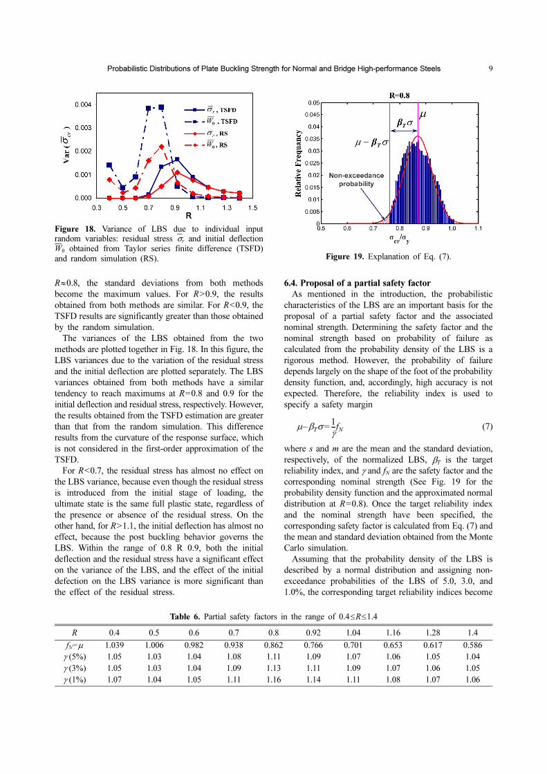
The variances of the LBS obtained from the two

methods are plotted together in Fig. 18. In this figure, the

LBS variances due to the variation of the residual stress

and the initial deflection are plotted separately. The LBS

variances obtained from both methods have a similar

tendency to reach maximums at R=0.8 and 0.9 for the

initial deflection and residual stress, respectively. However,

the results obtained from the TSFD estimation are greater

than that from the random simulation. This difference

results from the curvature of the response surface, which

is not considered in the first-order approximation of the

TSFD.

For R<0.7, the residual stress has almost no effect on

the LBS variance, because even though the residual stress

is introduced from the initial stage of loading, the

ultimate state is the same full plastic state, regardless of

the presence or absence of the residual stress. On the

other hand, for R>1.1, the initial deflection has almost no

effect, because the post buckling behavior governs the

LBS. Within the range of 0.8 R 0.9, both the initial

deflection and the residual stress have a significant effect

on the variance of the LBS, and the effect of the initial

defection on the LBS variance is more significant than

the effect of the residual stress.

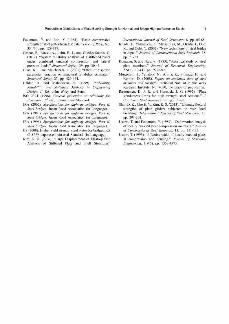
6.4. Proposal of a partial safety factor

As mentioned in the introduction, the probabilistic

characteristics of the LBS are an important basis for the

proposal of a partial safety factor and the associated

nominal strength. Determining the safety factor and the

nominal strength based on probability of failure as

calculated from the probability density of the LBS is a

rigorous method. However, the probability of failure

depends largely on the shape of the foot of the probability

density function, and, accordingly, high accuracy is not

expected. Therefore, the reliability index is used to

specify a safety margin

(7)

where s and m are the mean and the standard deviation,

respectively, of the normalized LBS, βT is the target

reliability index, and γ and fN are the safety factor and the

corresponding nominal strength (See Fig. 19 for the

probability density function and the approximated normal

distribution at R=0.8). Once the target reliability index

and the nominal strength have been specified, the

corresponding safety factor is calculated from Eq. (7) and

the mean and standard deviation obtained from the Monte

Carlo simulation.

Assuming that the probability density of the LBS is

described by a normal distribution and assigning non-

exceedance probabilities of the LBS of 5.0, 3.0, and

1.0%, the corresponding target reliability indices become

µ βTσ–1

γ---fN=

Figure 18. Variance of LBS due to individual inputrandom variables: residual stress σr and initial deflection

W0 obtained from Taylor series finite difference (TSFD)

and random simulation (RS).

Table 6. Partial safety factors in the range of 0.4≤R≤1.4

R 0.4 0.5 0.6 0.7 0.8 0.92 1.04 1.16 1.28 1.4

fN=µ 1.039 1.006 0.982 0.938 0.862 0.766 0.701 0.653 0.617 0.586

γ (5%) 1.05 1.03 1.04 1.08 1.11 1.09 1.07 1.06 1.05 1.04

γ (3%) 1.05 1.03 1.04 1.09 1.13 1.11 1.09 1.07 1.06 1.05

γ (1%) 1.07 1.04 1.05 1.11 1.16 1.14 1.11 1.08 1.07 1.06

Figure 19. Explanation of Eq. (7).


1.64, 1.88, and 2.33. Furthermore, setting the nominal

LBS to be equal to the mean of the LBS as an example,

the partial safety factor can be obtained as shown in Table

6.

As shown in Fig. 20, the maximum partial safety factor

values for exceedance probabilities of 5, 3, and 1% are

1.11, 1.13, and 1.16, respectively.

Calculating the partial safety factors for exceedance

probabilities of 5, 3, and 1% and assuming that the mean

LBS values are the nominal resistances, the obtained

design LBSs are compared to the corresponding design

values as specified by AASHTO (2007) and presented in

Fig. 21. As shown in the figure, the mean strengths

obtained in the present study are significantly lower than

the nominal strengths specified by AASHTO (2007)

within the range of 0.65<R<1.20.

7. Conclusion

The mean results of the LBS obtained from approximate

random simulation are similar to the mean curve reported

by Fukumoto and Itoh (1984) based on experimental data.

Compared with the standard deviation obtained from

the experimental results of Fukumoto and Itoh (1984), the

standard deviation based on the approximate random

simulation of the present study is approximately half for

0.6<R<1.2 and is significantly lower for R<0.6. The

causes of this significant difference are summarized as

follows: (a) the difference of the boundary condition

between experiments and numerical simulation; (b) the

variation of stress-strain relationship; and (c) the consideration

of the maximum initial deflection in the random simulation

in accordance with the design code.

The results of M-2S curve of the present study indicate

that the proposed JSHB design equation for steel plates in

compression is not conservative for 0.5<R<0.8 and is

overly conservative for R>0.85.

The M-2S curve proposed by Fukumoto and Itoh (1984)

is overly conservative compared to the corresponding

results of the present study.

Based on the LBS variance results obtained from the

three methods discussed herein, we have the following

conclusions regarding the influences of residual stress

and initial deflection on the LBS of steel plates:

-In the range of R<0.8, the influence of initial deflection

on the LBS of steel plates is more sensitive than that of

residual stress.

-In the range of R>0.9, the influence of residual stress

on the LBS of steel plates is more sensitive than that of

initial deflection.

-Within the range of 0.8<R<0.9, the influence of initial

deflection on the LBS of steel plates is dominant.

For R<0.5, the hardening behavior of steels significantly

affects the LBS of steel plates.

The approximation of response surface shows a very

good fit with the FEM results.

References

Bijlaard, F., Sedlacek, G., Muller, C., and Trumpf, H. (2003).

“Unified European design rules for steel and composite

structures.” International Journal of Steel Structures, 3,

pp. 117-125.

Dassault (2008). Abaqus Theory Manual v.6.8-EF. Dassault

Systemes Simulia Corp., the place of publication.

AASHTO (2007). AASHTO LRFD bridge design specifications.

4th Ed., American Association of State Highway and

Transportation Officials.

Eurocode 3 (2004). Design of steel structures. Parts 1-5.

Plated structural elements. European Committee for

Standardization (CEN), Brussels, Belgium.

Eurocode 4 (1994). Design of composite steel and concrete

structures. Part 2. General rules and rules for bridges.

European Committee for Standardization (CEN), Brussels,

Belgium.

Dwight, J. B. and Moxham, K. E. (1969). “Welded steel

plates in compression.” The Structural Engineer, 47(2),

pp. 49-66.

Figure 20. Partial safety factors obtained in the range of0.4≤R≤1.4

Figure 21. Design LBS for three levels of exceedanceprobability: 5, 3, and 1%, obtained in the present studyand corresponding design values as specified by AASHTO(2007).


Fukumoto, Y. and Itoh, Y. (1984). “Basic compressive

strength of steel plates from test data.” Proc. of JSCE, No.

334/I-1, pp. 129-139.

Gaspar, B., Naess, A., Leira, B. J., and Guedes Soares, C.

(2012). “System reliability analysis of a stiffened panel

under combined uniaxial compression and lateral

pressure loads.” Structural Safety, 39, pp. 30-43.

Guan, X. L. and Melchers R. E. (2001). “Effect of response

parameter variation on structural reliability estimates.”

Structural Safety, 23, pp. 429-444.

Haldar, A. and Mahadevan, S. (1999). Probability,

Reliability, and Statistical Methods in Engineering

Design. 1st Ed., John Wiley and Sons.

ISO 2394 (1998). General principles on reliability for

structures. 3rd Ed., International Standard.

JRA (2002). Specifications for highway bridges. Part II.

Steel bridges. Japan Road Association (in Language).





JIS (2008). Higher yield strength steel plates for bridges. JIS

G 3140, Japanese Industrial Standard (in Language).

Kim, K. D. (2006). “Large Displacement of Elasto-plastic

Analysis of Stiffened Plate and Shell Structures”

International Journal of Steel Structures, 6, pp. 65-68.

Kitada, T., Yamaguchi, T., Matsumura, M., Okada, J., Ono,

K., and Ochi, N. (2002). “New technology of steel bridge

in Japan.” Journal of Constructional Steel Research, 58,

pp. 21-70.

Komatsu, S. and Nara, S. (1983). “Statistical study on steel

plate members.” Journal of Structural Engineering,

ASCE, 109(4), pp. 977-992.

Murakoshi, J., Yanatory, N., Arima, K., Shimizu, H., and

Komori, D. (2008). Report on statistical data of steel

members and strength. Technical Note of Public Work

Research Institute, No. 4090, the place of publication.

Rasmussen, K. J. R. and Hancock, J. G. (1992). “Plate

slenderness limits for high strength steel sections.” J.

Construct. Steel Research. 23, pp. 73-96.

Shin, D. K., Cho E. Y., Kim, K. S. (2013). “Ultimate flexural

strengths of plate girders subjected to web local

buckling.” International Journal of Steel Structures, 13,

pp. 291-303.

Usami, T. and Fukumoto, Y. (1989). “Deformation analysis

of locally buckled steel compression members.” Journal

of Constructional Steel Research, 13, pp. 111-135.

Usami, T. (1993). “Effective width of locally buckled plates

in compression and bending.” Journal of Structural

Engineering, 119(5), pp. 1358-1373.

Documents

KSSC13-3(0)13-064