Kyun Queue: A Sensor Network System To Monitor Road …

Kyun Queue: A Sensor Network System To Monitor Road TrafficQueues

Rijurekha Sen, Abhinav Maurya, Bhaskaran Raman, Rupesh Mehta,Ramakrishnan Kalyanaraman, Nagamanoj Vankadhara, Swaroop Roy, Prashima Sharma

{riju, ahmaurya, br, rupeshm, krishnan, nagamanojv}@cse.iitb.ac.in,{bswarooproy, prashimasharma}@gmail.com

Indian Institute of Technology, Bombay

AbstractUnprecedented rate of growth in the number of vehicles

has resulted in acute road congestion problems worldwide.Better traffic flow management, based on enhanced trafficmonitoring, is being tried by city authorities. In many de-veloping countries, the situation is worse because of greaterskew in growth of traffic vs the road infrastructure. Further,the existing traffic monitoring techniques perform poorly inthe chaotic non-lane based traffic here.

In this paper, we presentKyun1 Queue, a sensor networksystem for real time traffic queue monitoring. Compared toexisting systems, it has several advantages: it (a) works inchaotic traffic, (b) does not interrupt traffic flow during itsinstallation and maintenance and (c) incurs low cost. Ourcontributions in this paper are four-fold. (1) We proposea new mechanism to sense road occupancy based on vari-ation in RF link characteristics, when line of sight betweena transmitter-receiver pair is obstructed. (2) We design algo-rithms to classify traffic states into congested or free-flowingat time scales of 20 seconds with above 90% accuracy. (3)We design and implement the embedded platforms neededto do the sensing, computation and communication to forma network of sensors. This network can correlate the trafficstate classification decisions of individual sensors, to detectmultiple levels of traffic congestion or traffic queue lengthon a given stretch of road, in real time. (4) Deployment ofour system on a Mumbai road, after careful consideration ofissues like localization and interference, gives correct esti-mates of traffic queue lengths, validated against 9 hours ofimage-based ground truth. Our system can provide input toseveral traffic management applications like traffic light con-trol, incident detection, and congestion monitoring.

1kyun, pronounced as ’few’ starting with ’k’ instead of ’f’, means ’why’in Hindi

Permission to make digital or hard copies of all or part of this work for personal orclassroom use is granted without fee provided that copies are not made or distributedfor profit or commercial advantage and that copies bear this notice and the full citationon the first page. To copy otherwise, to republish, to post on servers or to redistributeto lists, requires prior specific permission and/or a fee.

SenSys’12,November 6–9, 2012, Toronto, ON, Canada.Copyright c© 2012 ACM 978-1-4503-1169-4 ...$10.00

1 IntroductionThe problem of road congestion is currently plaguing

most cities in the world. Long traffic queues at signalizedintersections cause unpredictable travel times and fuel inef-ficiency [1, 2]. The problem is felt more acutely in grow-ing economies like India, primarily because infrastructuregrowth is slow compared to the growth in vehicles due tospace and cost constraints.

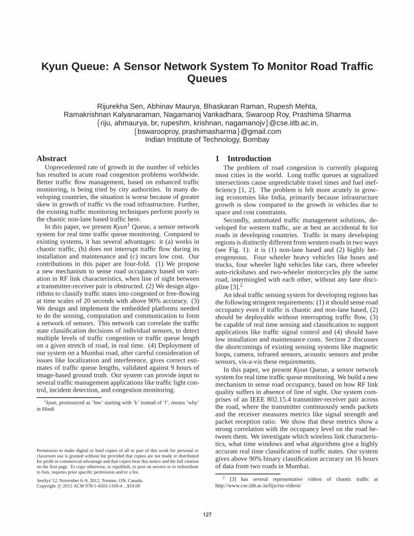
Secondly, automated traffic management solutions, de-veloped for western traffic, are at best an accidental fit forroads in developing countries. Traffic in many developingregions is distinctly different from western roads in two ways(see Fig. 1): it is (1) non-lane based and (2) highly het-erogeneous. Four wheeler heavy vehicles like buses andtrucks, four wheeler light vehicles like cars, three wheelerauto-rickshaws and two-wheeler motorcycles ply the sameroad, intermingled with each other, without any lane disci-pline [3].2

An ideal traffic sensing system for developing regions hasthe following stringent requirements: (1) it should sense roadoccupancy even if traffic is chaotic and non-lane based, (2)should be deployable without interrupting traffic flow, (3)be capable of real time sensing and classification to supportapplications like traffic signal control and (4) should havelow installation and maintenance costs. Section 2 discussesthe shortcomings of existing sensing systems like magneticloops, camera, infrared sensors, acoustic sensors and probesensors, vis-a-vis these requirements.

In this paper, we presentKyunQueue, a sensor networksystem for real time traffic queue monitoring. We build a newmechanism to sense road occupancy, based on how RF linkquality suffers in absence of line of sight. Our system com-prises of an IEEE 802.15.4 transmitter-receiver pair acrossthe road, where the transmitter continuously sends packetsand the receiver measures metrics like signal strength andpacket reception ratio. We show that these metrics show astrong correlation with the occupancy level on the road be-tween them. We investigate which wireless link characteris-tics, what time windows and what algorithms give a highlyaccurate real time classification of traffic states. Our systemgives above 90% binary classification accuracy on 16 hoursof data from two roads in Mumbai.

2 [3] has several representative videos of chaotic traffic athttp://www.cse.iitb.ac.in/riju/rss-videos/

127

Figure 1: Chaotic traffic (source [4]) Figure 2: Lane based traffic Figure 3: Issues with infrared

Building on this binary classification of traffic states us-ing one pair of sensors, we construct a linear array of suchsensors. This can detect the length of a queue or the de-gree of congestion on a given road stretch. We design andbuild appropriate embedded platforms to do (1) sensing andcomputation for binary classification, (2) communication tocombine the decisions of multiple sensors to know the lengthof traffic queue and (3) communication of the queue lengthvalues to a remote server.

Our system, deployed on a Mumbai road for 9 hours, pe-riodically (every 30 secs in our deployment) reports trafficqueue length values to a remote server. Manual examinationof the corresponding 9 hours of image-based ground truth,gives maximum accuracy of our queue estimates to be 96%and minimum accuracy to be 74%. These queue estimatescan be potentially used in a range of applications such as:automating traffic light control, detecting bottlenecks or cre-ating congestion maps of a city.

The rest of the paper is organized as follows. Section 2discusses the existing traffic sensing solutions. Our proposedsensing technique and the real time traffic state classifica-tion algorithms based on it, are discussed in Section 3. Thedesign of our sensor network is detailed in Section 4 andhardware prototypes are described in Section 5. We presentthe deployment based evaluation of our system in Section 6.Finally we discuss the issues of sensor localization, interfer-ence and power consumption, before concluding the paper.

2 Related workAutomated traffic management solutions have been de-

ployed in many developed countries since several years. Inthis section, we discuss the traffic sensing methods primarilyused to provide input to the traffic management systems andtheir usability in chaotic traffic.

Loop detectors -There are a lot of research projects [5, 7]and several deployed systems [6] that do vehicle counting us-ing magnetic loops under the road. A vehicle loop detectorcosts $700 for a loop, $2500 for a controller, $5000 for acontroller cabinet and 10% of the original installation costfor annual maintenance [1]. Loops need to be placed underthe road. Digging up roads to install and maintain the in-frastructure intrudes into traffic flow. Also re-laying the roadsurface needs re-laying the sensors. Moreover, loops havebeen traditionally placed under each lane as seen in Fig. 2(a).How should the placement be in absence of lanes is yet to beexplored.

In comparison, our sensors are to be placed on roadside,

without affecting the flow of traffic. We can sense road occu-pancy even if traffic is chaotic and non-lane based. Our tech-nique is cheap, with each sensor pair costing about $200.This is the cost of prototype using off-the-shelf modules,which can further reduce with customized design. Each pairgives a binary classification of traffic state as free-flow orcongested. To know length of queue, we need an array ofsensor pairs. We can cover about 200 meters of road at about$1200.

Image sensors -Video surveillance based traffic moni-toring is fairly common [8]. [17] gives a comprehensive sur-vey of the major computer vision techniques used in trafficapplications. But the traditional setting for which vision al-gorithms exist can be seen in Fig. 2(b). For usability in de-veloping countries, algorithms are needed for scenarios likeFig. 1. [18] is a preliminary work on image processing algo-rithms for chaotic traffic sensing. The algorithms are offline,so the trade-off between computation and communication isnot yet understood. Also the sensing accuracy itself has beentested on only 2 minutes of video clip. [19] is another re-cent work to use low quality images from CCTV for traf-fic sensing. But computational overhead, real-timeliness andaccuracy of the designed algorithms are yet to be evaluated.Thus though image-based sensing shows promise, with ad-vantages such as ease of deployment and potential low cost,there are several aspects that need careful evaluation and val-idation, especially in chaotic traffic conditions.

In comparison, we present an alternative traffic sensingsystem that works in chaotic non-lane based traffic. We havethoroughly evaluated the sensing accuracy on 16 hours oftraffic in Mumbai. The algorithms are very low overheadand we have implemented them on low end embedded sensorplatforms. Sensing and computation are done on the road.Only the traffic queue length values are communicated tothe remote server, avoiding the communication overhead ofvideo transfer.

Infrared sensors -Active infrared sensors placed acrossthe road suffer beam cuts by vehicular movement in be-tween. [10] is a commercial product that measures speed,length and lanes of vehicles from beam cuts. However, in-frared propagates as a ray, and hence is strictly line of sight(LOS) based. This makes it overly sensitive to even smallobstacles. When we tried using it on Mumbai roads, pedes-trians who frequently use the roads (Fig. 3(a)) or irregulari-ties of the road surface (Fig. 3(b)) would not allow the tx-rxpair to communicate. Also [10] has been tested only in lane-based traffic. Beam cuts in high density, non-lane based and

128

Technique Drawbacksloop detectors [5, 6], high cost, under-the-road installation,magnetic sensors [7] do not currently support chaotic traffic

video and images [8, 9] attractive option for exploration,but no proven solutions for chaotic traffic thus far

potentially high computation and/orcommunication overhead for chaotic traffic

IR sensors [10] pedestrians, road surface irregularities and non-lanebased vehicular movement cause spurious beam cuts

acoustic sensors [11, 12, 3] high training overhead, slow responseprobe sensors [1, 13, 14, 15, 16] useful for complementary applications,

but too sparse and noisy to allow micro management of road networks

Table 1: Drawbacks of existing techniques for chaotic traffic management

heterogeneous traffic as seen in Fig. 1, would need carefulstudy to be used for chaotic traffic measurement.

The setup of sensor pair across road in our system uses802.15.4 radios which have a spread propagation model, in-stead of ray propagation model of infrared. This makes ourtechnique robust to noise and thus suitable for disorderlyroad conditions such as in Fig. 1. This robustness is evidentfrom the rigorous empirical evaluation of our binary trafficstate classification over 16 hours of chaotic traffic data. Wealso enhance the pairwise sensing to an array of sensors anddetect length of queues, an aspect not examined in the IR-based systems.

Acoustic sensors -Some recent research is being done touse acoustic sensors for traffic state estimation, especially indeveloping regions, where traffic being chaotic is noisy [12].But standing traffic does not have any uniform sound sig-nature and depends largely on the driver behavior and typeof vehicles. For example, if vehicles are standing in a longqueue awaiting a green signal, many drivers might just shutdown the engines and wait silently or might blow honk im-patiently, producing two very different sound signatures forsame traffic state. This reduces the sensing accuracy [3].Also, to attain a valid signature correlating to a traffic state,sensing time window of at least a minute or so is needed,making these systems slow in response.

In comparison, our technique works in the order of 10-20 seconds. The classification accuracy is also much higherthan acoustic, as vehicles being heavy metallic obstacles al-ways affect RF signal quality. This high accuracy also makesit possible, to take the binary classification to a multilevelclassification using an array of RF sensors to know length ofqueue on a road. Achieving this with low accuracy acousticsensors would be tricky.

Probe sensors -Significant research is being done toleverage cell phones and participatory sensing to generatetraffic related information. Focus has been given to researchboth in networking issues [20, 21, 22] and machine learningissues [23, 1, 15]. But participatory sensing data is inher-ently noisy [24]. Also probe vehicles might not be present ata given intersection at all times. Travel time estimates, transitvehicle information and congestion maps to be disseminatedto commuters for route selection, can tolerate aperiodicityand noise. Such commuter applications are thus highly suit-

able using probe data.Our work is aimed at providing strictly periodic, accu-

rate input to traffic management systems. Our system, basedon static sensors, would potentially be used at some keyintersections of a city, where intelligent and adaptive con-trol would positively affect traffic flow. This is orthogonaland complementary to the commuter applications handledby probe sensing.

The drawbacks of existing techniques are summarized inTable 1. Some techniques like loops and acoustic sensinghave clear disadvantages. Some like probe sensors are ill-suited for the particular applications that we are targetingin this paper. Some others like image and infrared sensingmight work after adaptation for chaotic traffic, but there isno working adaptation till date.

3 Traffic sensing with wireless across roadIn this paper, we wish to design a system for traffic queue

length measurement in chaotic road conditions. This has sev-eral potential applications like traffic light control, incidentdetection, and congestion monitoring. An important pointto note here is that, at almost all intersections in developingcountries, a variety of vehicles stand as a coagulated masswaiting for green signal (see Fig. 1). On getting green sig-nal, they all move forward almost bumper to bumper, withlittle variability in speeds. So queue length is proportionalto traffic volume, the road width being the proportionalityconstant. We thus assume, as is intuitive, that finer granu-larity information like exact vehicle counts are unnecessary.To tune traffic lights proportional to waiting traffic volumes,queue lengths are sufficient. Thus we aim to detect roadoccupancy in chaotic traffic, and build upon that to detectlength of queues.

It is well known in the wireless networking domain, thatcharacteristics of wireless links like 802.11 and 802.15.4 areaffected in the absence of LOS [25]. Obstacles cause reflec-tion, absorption and scattering of the RF signal, degradingthe link quality. Researchers have exploited these vagaries ofRF links in different kinds of application scenarios, the mostcommon being that for indoor localization [26, 27, 28, 29].

The effects of vehicular traffic on wireless links werebriefly studied in [30], where the authors seeked to quantifythe link quality in harsh deployment scenarios, like tunnels

129

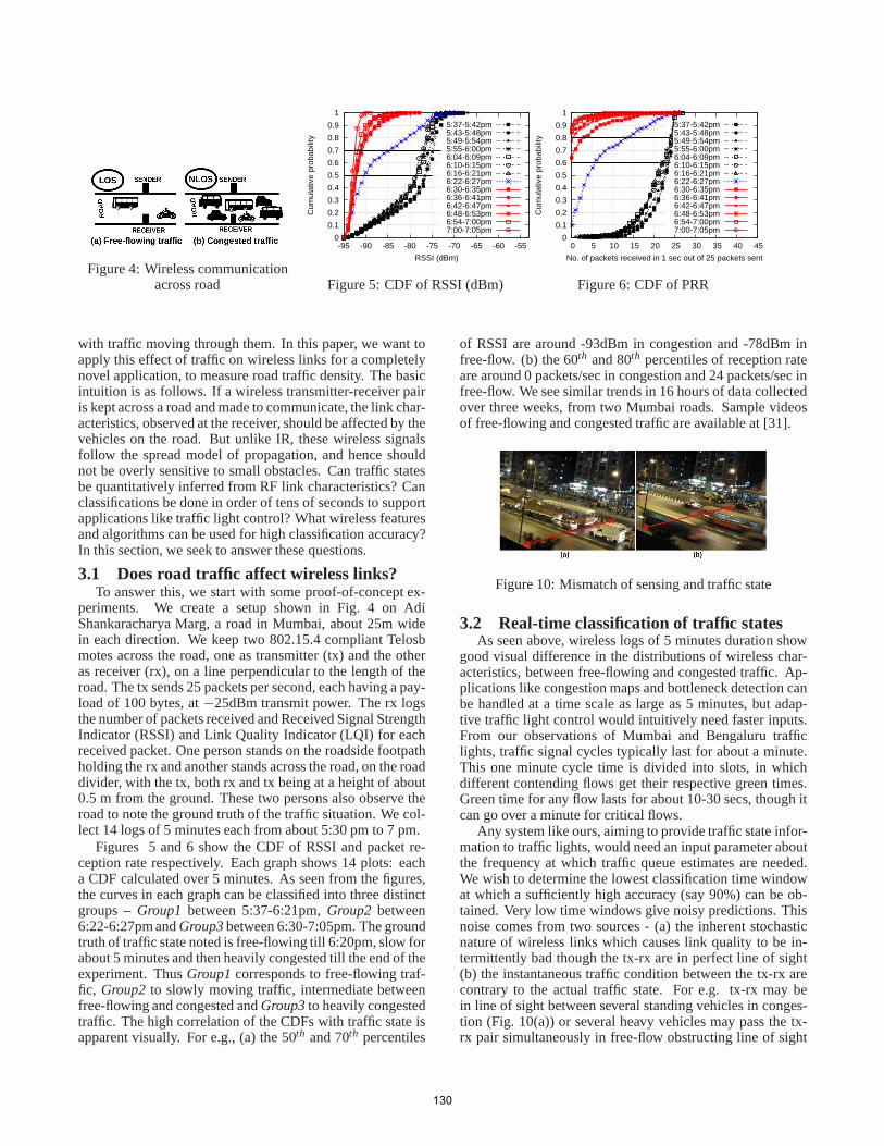
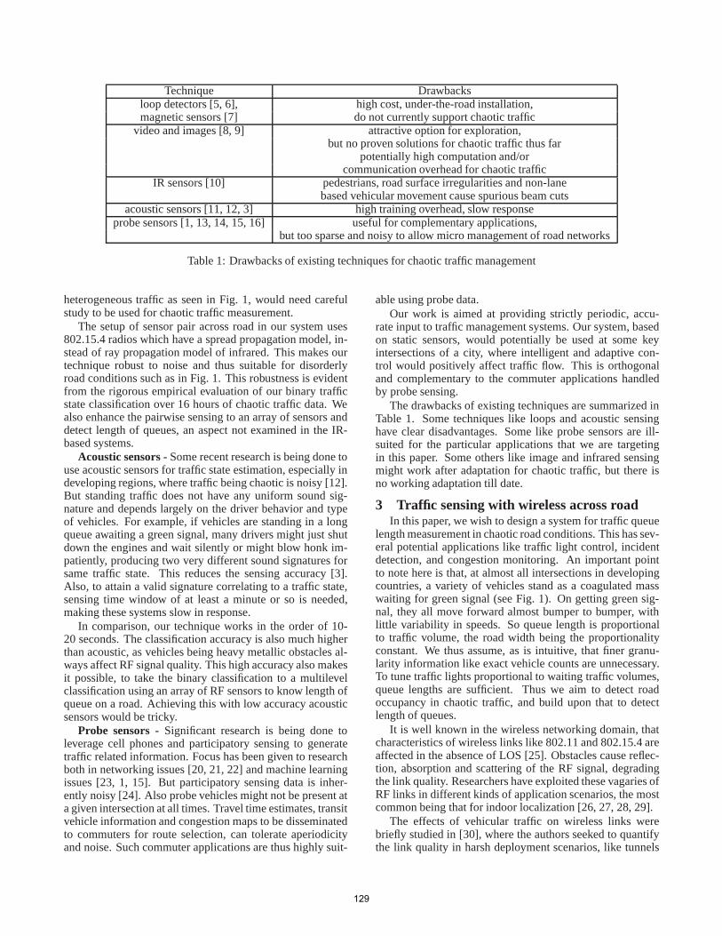
Figure 4: Wireless communicationacross road

0

0.1

0.2

0.3

0.4

0.5

0.6

0.7

0.8

0.9

1

-95 -90 -85 -80 -75 -70 -65 -60 -55

Cum

ulat

ive

prob

abili

ty

RSSI (dBm)

5:37-5:42pm5:43-5:48pm5:49-5:54pm5:55-6:00pm6:04-6:09pm6:10-6:15pm6:16-6:21pm6:22-6:27pm6:30-6:35pm6:36-6:41pm6:42-6:47pm6:48-6:53pm6:54-7:00pm7:00-7:05pm

Figure 5: CDF of RSSI (dBm)

0

0.1

0.2

0.3

0.4

0.5

0.6

0.7

0.8

0.9

1

0 5 10 15 20 25 30 35 40 45

Cum

ulat

ive

prob

abili

ty

No. of packets received in 1 sec out of 25 packets sent

5:37-5:42pm5:43-5:48pm5:49-5:54pm5:55-6:00pm6:04-6:09pm6:10-6:15pm6:16-6:21pm6:22-6:27pm6:30-6:35pm6:36-6:41pm6:42-6:47pm6:48-6:53pm6:54-7:00pm7:00-7:05pm

Figure 6: CDF of PRR

with traffic moving through them. In this paper, we want toapply this effect of traffic on wireless links for a completelynovel application, to measure road traffic density. The basicintuition is as follows. If a wireless transmitter-receiver pairis kept across a road and made to communicate, the link char-acteristics, observed at the receiver, should be affected by thevehicles on the road. But unlike IR, these wireless signalsfollow the spread model of propagation, and hence shouldnot be overly sensitive to small obstacles. Can traffic statesbe quantitatively inferred from RF link characteristics? Canclassifications be done in order of tens of seconds to supportapplications like traffic light control? What wireless featuresand algorithms can be used for high classification accuracy?In this section, we seek to answer these questions.

3.1 Does road traffic affect wireless links?To answer this, we start with some proof-of-concept ex-

periments. We create a setup shown in Fig. 4 on AdiShankaracharya Marg, a road in Mumbai, about 25m widein each direction. We keep two 802.15.4 compliant Telosbmotes across the road, one as transmitter (tx) and the otheras receiver (rx), on a line perpendicular to the length of theroad. The tx sends 25 packets per second, each having a pay-load of 100 bytes, at−25dBm transmit power. The rx logsthe number of packets received and Received Signal StrengthIndicator (RSSI) and Link Quality Indicator (LQI) for eachreceived packet. One person stands on the roadside footpathholding the rx and another stands across the road, on the roaddivider, with the tx, both rx and tx being at a height of about0.5 m from the ground. These two persons also observe theroad to note the ground truth of the traffic situation. We col-lect 14 logs of 5 minutes each from about 5:30 pm to 7 pm.

Figures 5 and 6 show the CDF of RSSI and packet re-ception rate respectively. Each graph shows 14 plots: eacha CDF calculated over 5 minutes. As seen from the figures,the curves in each graph can be classified into three distinctgroups –Group1 between 5:37-6:21pm,Group2 between6:22-6:27pm andGroup3between 6:30-7:05pm. The groundtruth of traffic state noted is free-flowing till 6:20pm, slow forabout 5 minutes and then heavily congested till the end of theexperiment. ThusGroup1corresponds to free-flowing traf-fic, Group2 to slowly moving traffic, intermediate betweenfree-flowing and congested andGroup3to heavily congestedtraffic. The high correlation of the CDFs with traffic state isapparent visually. For e.g., (a) the 50th and 70th percentiles

of RSSI are around -93dBm in congestion and -78dBm infree-flow. (b) the 60th and 80th percentiles of reception rateare around 0 packets/sec in congestion and 24 packets/sec infree-flow. We see similar trends in 16 hours of data collectedover three weeks, from two Mumbai roads. Sample videosof free-flowing and congested traffic are available at [31].

Figure 10: Mismatch of sensing and traffic state

3.2 Real-time classification of traffic statesAs seen above, wireless logs of 5 minutes duration show

good visual difference in the distributions of wireless char-acteristics, between free-flowing and congested traffic. Ap-plications like congestion maps and bottleneck detection canbe handled at a time scale as large as 5 minutes, but adap-tive traffic light control would intuitively need faster inputs.From our observations of Mumbai and Bengaluru trafficlights, traffic signal cycles typically last for about a minute.This one minute cycle time is divided into slots, in whichdifferent contending flows get their respective green times.Green time for any flow lasts for about 10-30 secs, though itcan go over a minute for critical flows.

Any system like ours, aiming to provide traffic state infor-mation to traffic lights, would need an input parameter aboutthe frequency at which traffic queue estimates are needed.We wish to determine the lowest classification time windowat which a sufficiently high accuracy (say 90%) can be ob-tained. Very low time windows give noisy predictions. Thisnoise comes from two sources - (a) the inherent stochasticnature of wireless links which causes link quality to be in-termittently bad though the tx-rx are in perfect line of sight(b) the instantaneous traffic condition between the tx-rx arecontrary to the actual traffic state. For e.g. tx-rx may bein line of sight between several standing vehicles in conges-tion (Fig. 10(a)) or several heavy vehicles may pass the tx-rx pair simultaneously in free-flow obstructing line of sight

130

6

8

10

12

14

16

18

20

10 20 30 40 50 60 0

2000

4000

6000

8000

10000

Err

or (

%)

Num

ber

of D

atap

oint

s

Prediction Time Window (seconds)

SVM Train ErrorK-Means Train Error

Number of Datapoints

Figure 7: FC algorithm training error

6

8

10

12

14

16

18

20

10 20 30 40 50 60 0

2000

4000

6000

8000

10000

Err

or (

%)

Num

ber

of D

atap

oint

s


SVM Train ErrorK-Means Train Error


Figure 8: SC algorithm training error

8

10

12

14

16

18

20

10 20 30 40 50 60 0

2000

4000

6000

8000

10000

Err

or (

%)

Num

ber

of D

atap

oint

s


RSSIRSSI, LQI

RSSI, PRRRSSI, LQI, PRR


Figure 9: Choice of features

(Fig. 10(b)). Thus we need to choose the classification timewindow, henceforth referred to ast, carefully.

3.3 Labeled data-set for evaluationTo evaluate our choices oft, features and algorithms

for real time traffic state classification, we need a data-setwith labeled ground truth. For this purpose, we use the16 hours data-set, collected using the setup in Fig. 4. Thedata is collected from two Mumbai roads, a 25 m wide AdiShankaracharya Marg, henceforth referred to as wide-roadand another road, 8 m in width, henceforth referred to as nar-row road. Specifically we have 13676 secs of wide-road datalabeled as free-flow and 14992 secs labeled as congested.Similarly, we have 13486 secs of narrow-road data labeled asfree-flow and 16678 secs labeled as congested. The labelingwas done at a larger time-scale of 5 minutes to reduce man-ual overhead and all the one second long windows, belongingto the same 5 minute window were uniformly labeled. Theroads and the times of day of data collection were chosenin a way that traffic states did not toggle within 5 minutes.Thus the error in ground truth observation, even if present,is very small. Representative videos, showing free-flow andcongested traffic on the wide road, can be found at [31].

3.4 Classification algorithmsWe use machine learning algorithms to do traffic state

classification. In this paper, we concentrate onbinary traf-fic state classification:congested traffic, when vehicles haveto brake and stop vsfree-flowing traffic, when vehicles moveaccording to the driver’s intended speed, bounded by the roadspeed limit. We show that this binary classification is suf-ficient for queue length estimation, using binary decisionsfrom a linear array of multiple sensor pairs.

To decide what binary classifier to use, the trade-off is be-tween (1) accuracy of classification, (2) implementability ona low end embedded platform, (3) complexity of the classi-fier models and (4) overhead of model training. Linear hy-perplane classifiers are simple enough to implement on ourplatform (TI’s C5505) and to train and test in near real time.SVM and K-Means-based classifiers belong to this categoryand are state-of-the-art supervized and unsupervized learn-ing algorithms respectively. K-Means, being unsupervized,has the additional advantage of minimal manual labeling oftraining data. We build four possible algorithms based onthese two classifiers and subsequently choose one based on

accuracy and labeling overhead.FeatureClassifier (FC) algorithm- In this algorithm, the

wireless data for a certaint is transformed into a feature vec-tor comprising 9 features: from the set of RSSI values ofpackets received in a time window, the nine percentile val-ues corresponding to 10th, 20th, ..., 90th percentile are drawnas features. The ground truth for the corresponding time win-dow is appended to the generated feature vector. If no packetis received in a time window, a dummy packet having RSSIof -95 dBm, close to the radio sensitivity level, is consideredto have been received. The collection of all data points thusobtained comprises the training dataset. This is used to trainclassification models either using SVM or K-Means. In thetesting phase, similar feature vectors are created from wire-less data over the same time windowt. Then eacht is labeledas free-flow or congested based on the training model.

SignalClassifier (SC) algorithm - This meta-classifieralternative to FeatureClassifier, uses majority voting on per-packet congestion predictions. In the training phase, we ob-tain a per-packet classifier using K-means or SVM, by con-sidering only the packet RSSI as a feature. In the testingphase, for eacht, we employ the per-packet classifier ob-tained in the training phase on each received packet, ob-

taining a label for each packet. Considercount(t)congestionand

count(t)f ree f low to be the number of packet-level congestionand free-flow predictions in a time slott. We predict con-

gestion in the time slot ifcount(t)congestionis greater than or

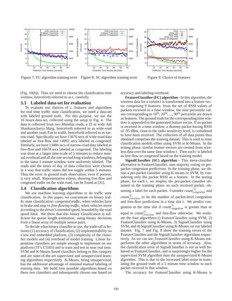
equal tocount(t)f ree f low and free-flow otherwise. We evalu-ate the four algorithms:1) FeatureClassifier using SVM, 2)FeatureClassifier using K-Means, 3) SignalClassifier usingSVM, and 4) SignalClassifier using K-Means, on our labeleddataset. Fig. 7 and Fig. 8 show the training errors of theFeatureClassifier and the SignalClassifier algorithms respec-tively. As we can see, FeatureClassifier using K-Means out-performs the other algorithms in terms of accuracy. Also,the classification error of SignalClassifier is not as well be-haved as FeatureClassifier, and is surprisingly higher for thesupervized SVM algorithm than the unsupervized K-Meansalgorithm. This is due to the increased label noise in trans-lating the ground truth of a 5 minute time window to eachpacket received in that window.

The accuracy for FeatureClassifier using K-Means is

131

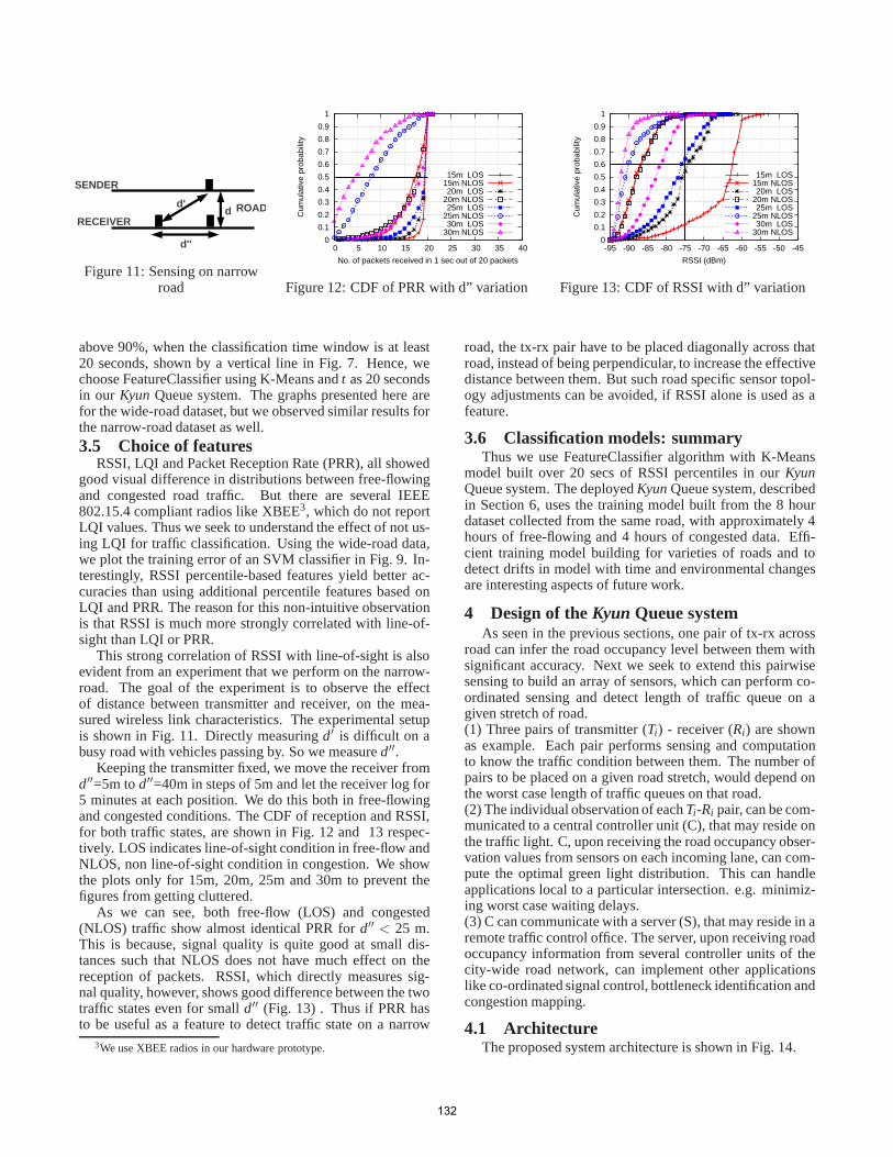
Figure 11: Sensing on narrowroad

0

0.1

0.2

0.3

0.4

0.5

0.6

0.7

0.8

0.9

1

0 5 10 15 20 25 30 35 40

Cum

ulat

ive

prob

abili

ty

No. of packets received in 1 sec out of 20 packets

15m LOS15m NLOS20m LOS

20m NLOS25m LOS

25m NLOS30m LOS

30m NLOS

Figure 12: CDF of PRR with d” variation

0

0.1

0.2

0.3

0.4

0.5

0.6

0.7

0.8

0.9

1

-95 -90 -85 -80 -75 -70 -65 -60 -55 -50 -45

Cum

ulat

ive

prob

abili

ty

RSSI (dBm)

15m LOS15m NLOS20m LOS

20m NLOS25m LOS

25m NLOS30m LOS

30m NLOS

Figure 13: CDF of RSSI with d” variation

above 90%, when the classification time window is at least20 seconds, shown by a vertical line in Fig. 7. Hence, wechoose FeatureClassifier using K-Means andt as 20 secondsin our Kyun Queue system. The graphs presented here arefor the wide-road dataset, but we observed similar results forthe narrow-road dataset as well.3.5 Choice of features

RSSI, LQI and Packet Reception Rate (PRR), all showedgood visual difference in distributions between free-flowingand congested road traffic. But there are several IEEE802.15.4 compliant radios like XBEE3, which do not reportLQI values. Thus we seek to understand the effect of not us-ing LQI for traffic classification. Using the wide-road data,we plot the training error of an SVM classifier in Fig. 9. In-terestingly, RSSI percentile-based features yield better ac-curacies than using additional percentile features based onLQI and PRR. The reason for this non-intuitive observationis that RSSI is much more strongly correlated with line-of-sight than LQI or PRR.

This strong correlation of RSSI with line-of-sight is alsoevident from an experiment that we perform on the narrow-road. The goal of the experiment is to observe the effectof distance between transmitter and receiver, on the mea-sured wireless link characteristics. The experimental setupis shown in Fig. 11. Directly measuringd′ is difficult on abusy road with vehicles passing by. So we measured′′.

Keeping the transmitter fixed, we move the receiver fromd′′=5m tod′′=40m in steps of 5m and let the receiver log for5 minutes at each position. We do this both in free-flowingand congested conditions. The CDF of reception and RSSI,for both traffic states, are shown in Fig. 12 and 13 respec-tively. LOS indicates line-of-sight condition in free-flow andNLOS, non line-of-sight condition in congestion. We showthe plots only for 15m, 20m, 25m and 30m to prevent thefigures from getting cluttered.

As we can see, both free-flow (LOS) and congested(NLOS) traffic show almost identical PRR ford′′

< 25 m.This is because, signal quality is quite good at small dis-tances such that NLOS does not have much effect on thereception of packets. RSSI, which directly measures sig-nal quality, however, shows good difference between the twotraffic states even for smalld′′ (Fig. 13) . Thus if PRR hasto be useful as a feature to detect traffic state on a narrow

3Weuse XBEE radios in our hardware prototype.

road, the tx-rx pair have to be placed diagonally across thatroad, instead of being perpendicular, to increase the effectivedistance between them. But such road specific sensor topol-ogy adjustments can be avoided, if RSSI alone is used as afeature.

3.6 Classification models: summaryThus we use FeatureClassifier algorithm with K-Means

model built over 20 secs of RSSI percentiles in ourKyunQueue system. The deployedKyunQueue system, describedin Section 6, uses the training model built from the 8 hourdataset collected from the same road, with approximately 4hours of free-flowing and 4 hours of congested data. Effi-cient training model building for varieties of roads and todetect drifts in model with time and environmental changesare interesting aspects of future work.

4 Design of theKyun Queue systemAs seen in the previous sections, one pair of tx-rx across

road can infer the road occupancy level between them withsignificant accuracy. Next we seek to extend this pairwisesensing to build an array of sensors, which can perform co-ordinated sensing and detect length of traffic queue on agiven stretch of road.(1) Three pairs of transmitter (Ti) - receiver (Ri) are shownas example. Each pair performs sensing and computationto know the traffic condition between them. The number ofpairs to be placed on a given road stretch, would depend onthe worst case length of traffic queues on that road.(2) The individual observation of eachTi-Ri pair, can be com-municated to a central controller unit (C), that may reside onthe traffic light. C, upon receiving the road occupancy obser-vation values from sensors on each incoming lane, can com-pute the optimal green light distribution. This can handleapplications local to a particular intersection. e.g. minimiz-ing worst case waiting delays.(3) C can communicate with a server (S), that may reside in aremote traffic control office. The server, upon receiving roadoccupancy information from several controller units of thecity-wide road network, can implement other applicationslike co-ordinated signal control, bottleneck identification andcongestion mapping.

4.1 ArchitectureThe proposed system architecture is shown in Fig. 14.

132

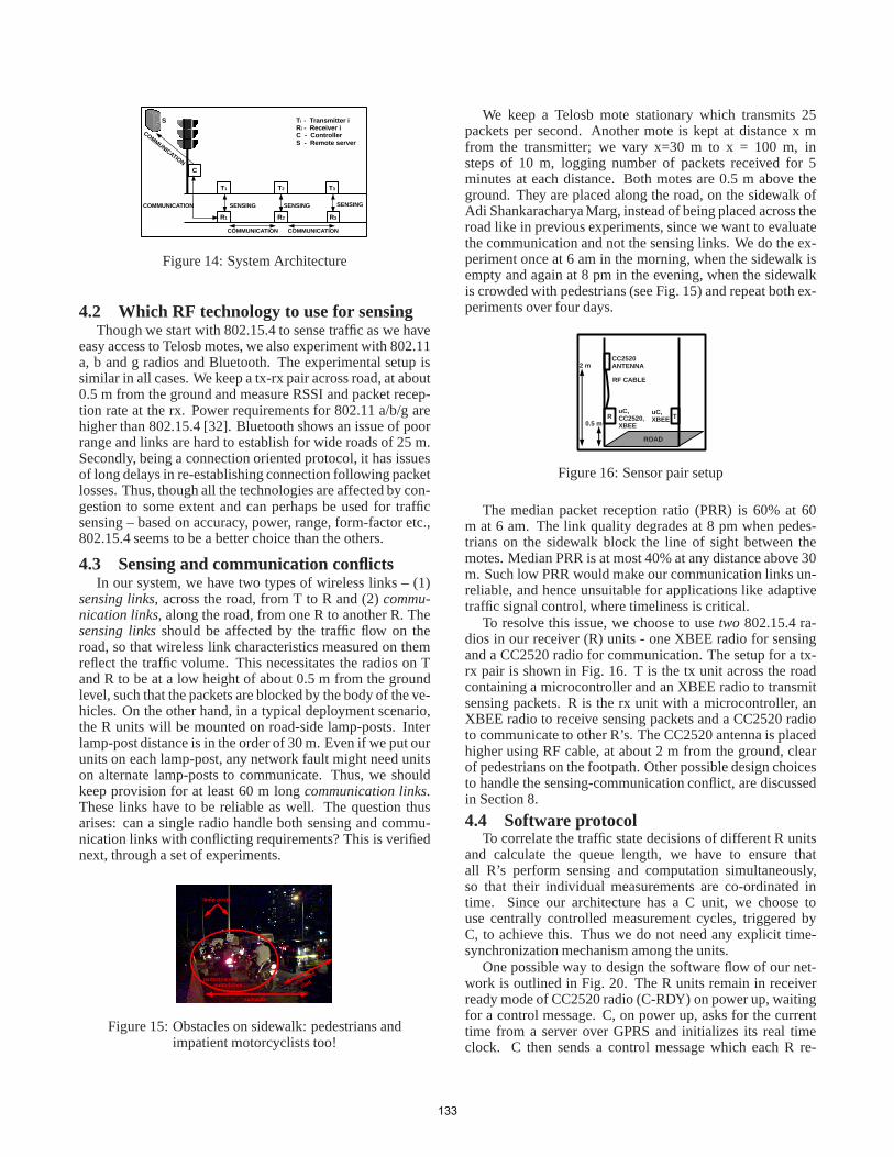
Figure 14: System Architecture

4.2 Which RF technology to use for sensingThough we start with 802.15.4 to sense traffic as we have

easy access to Telosb motes, we also experiment with 802.11a, b and g radios and Bluetooth. The experimental setup issimilar in all cases. We keep a tx-rx pair across road, at about0.5 m from the ground and measure RSSI and packet recep-tion rate at the rx. Power requirements for 802.11 a/b/g arehigher than 802.15.4 [32]. Bluetooth shows an issue of poorrange and links are hard to establish for wide roads of 25 m.Secondly, being a connection oriented protocol, it has issuesof long delays in re-establishing connection following packetlosses. Thus, though all the technologies are affected by con-gestion to some extent and can perhaps be used for trafficsensing – based on accuracy, power, range, form-factor etc.,802.15.4 seems to be a better choice than the others.

4.3 Sensing and communication conflictsIn our system, we have two types of wireless links – (1)

sensing links, across the road, from T to R and (2)commu-nication links, along the road, from one R to another R. Thesensing linksshould be affected by the traffic flow on theroad, so that wireless link characteristics measured on themreflect the traffic volume. This necessitates the radios on Tand R to be at a low height of about 0.5 m from the groundlevel, such that the packets are blocked by the body of the ve-hicles. On the other hand, in a typical deployment scenario,the R units will be mounted on road-side lamp-posts. Interlamp-post distance is in the order of 30 m. Even if we put ourunits on each lamp-post, any network fault might need unitson alternate lamp-posts to communicate. Thus, we shouldkeep provision for at least 60 m longcommunication links.These links have to be reliable as well. The question thusarises: can a single radio handle both sensing and commu-nication links with conflicting requirements? This is verifiednext, through a set of experiments.

Figure 15: Obstacles on sidewalk: pedestrians andimpatient motorcyclists too!

We keep a Telosb mote stationary which transmits 25packets per second. Another mote is kept at distance x mfrom the transmitter; we vary x=30 m to x = 100 m, insteps of 10 m, logging number of packets received for 5minutes at each distance. Both motes are 0.5 m above theground. They are placed along the road, on the sidewalk ofAdi Shankaracharya Marg, instead of being placed across theroad like in previous experiments, since we want to evaluatethe communication and not the sensing links. We do the ex-periment once at 6 am in the morning, when the sidewalk isempty and again at 8 pm in the evening, when the sidewalkis crowded with pedestrians (see Fig. 15) and repeat both ex-periments over four days.

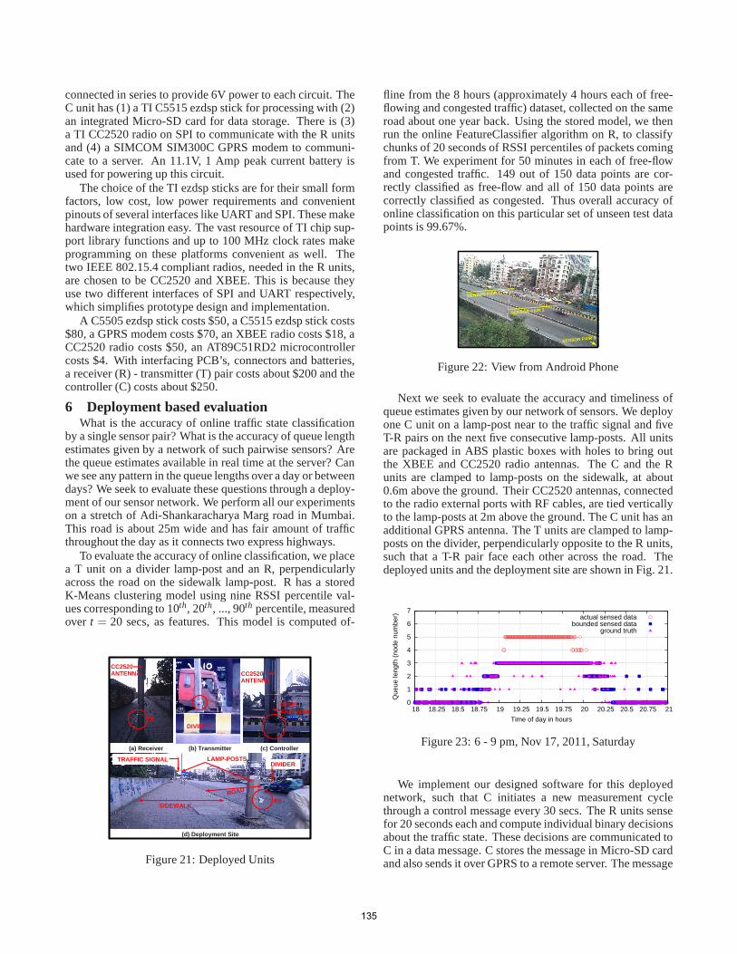
Figure 16: Sensor pair setup

The median packet reception ratio (PRR) is 60% at 60m at 6 am. The link quality degrades at 8 pm when pedes-trians on the sidewalk block the line of sight between themotes. Median PRR is at most 40% at any distance above 30m. Such low PRR would make our communication links un-reliable, and hence unsuitable for applications like adaptivetraffic signal control, where timeliness is critical.

To resolve this issue, we choose to usetwo 802.15.4 ra-dios in our receiver (R) units - one XBEE radio for sensingand a CC2520 radio for communication. The setup for a tx-rx pair is shown in Fig. 16. T is the tx unit across the roadcontaining a microcontroller and an XBEE radio to transmitsensing packets. R is the rx unit with a microcontroller, anXBEE radio to receive sensing packets and a CC2520 radioto communicate to other R’s. The CC2520 antenna is placedhigher using RF cable, at about 2 m from the ground, clearof pedestrians on the footpath. Other possible design choicesto handle the sensing-communication conflict, are discussedin Section 8.

4.4 Software protocolTo correlate the traffic state decisions of different R units

and calculate the queue length, we have to ensure thatall R’s perform sensing and computation simultaneously,so that their individual measurements are co-ordinated intime. Since our architecture has a C unit, we choose touse centrally controlled measurement cycles, triggered byC, to achieve this. Thus we do not need any explicit time-synchronization mechanism among the units.

One possible way to design the software flow of our net-work is outlined in Fig. 20. The R units remain in receiverready mode of CC2520 radio (C-RDY) on power up, waitingfor a control message. C, on power up, asks for the currenttime from a server over GPRS and initializes its real timeclock. C then sends a control message which each R re-

133

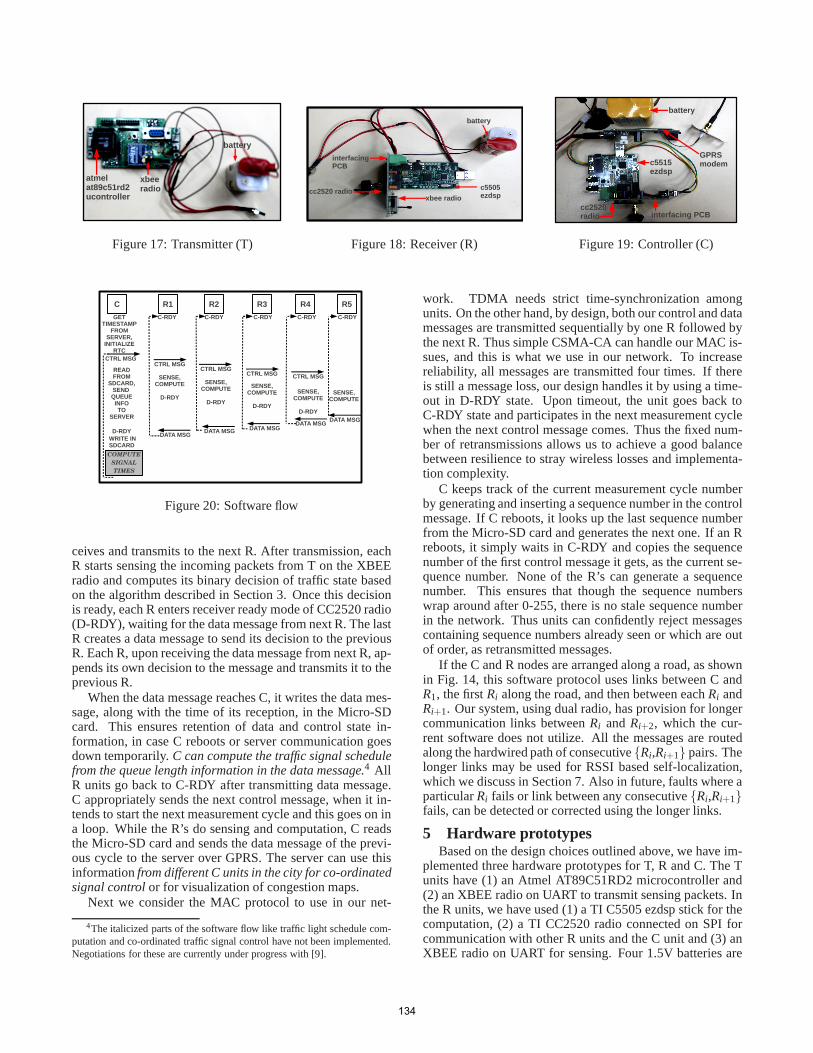
Figure 17: Transmitter (T) Figure 18: Receiver (R) Figure 19: Controller (C)

Figure 20: Software flow

ceives and transmits to the next R. After transmission, eachR starts sensing the incoming packets from T on the XBEEradio and computes its binary decision of traffic state basedon the algorithm described in Section 3. Once this decisionis ready, each R enters receiver ready mode of CC2520 radio(D-RDY), waiting for the data message from next R. The lastR creates a data message to send its decision to the previousR. Each R, upon receiving the data message from next R, ap-pends its own decision to the message and transmits it to theprevious R.

When the data message reaches C, it writes the data mes-sage, along with the time of its reception, in the Micro-SDcard. This ensures retention of data and control state in-formation, in case C reboots or server communication goesdown temporarily.C can compute the traffic signal schedulefrom the queue length information in the data message.4 AllR units go back to C-RDY after transmitting data message.C appropriately sends the next control message, when it in-tends to start the next measurement cycle and this goes on ina loop. While the R’s do sensing and computation, C readsthe Micro-SD card and sends the data message of the previ-ous cycle to the server over GPRS. The server can use thisinformationfrom different C units in the city for co-ordinatedsignal controlor for visualization of congestion maps.

Next we consider the MAC protocol to use in our net-

4The italicized parts of the software flow like traffic light schedule com-putation and co-ordinated traffic signal control have not been implemented.Negotiations for these are currently under progress with [9].

work. TDMA needs strict time-synchronization amongunits. On the other hand, by design, both our control and datamessages are transmitted sequentially by one R followed bythe next R. Thus simple CSMA-CA can handle our MAC is-sues, and this is what we use in our network. To increasereliability, all messages are transmitted four times. If thereis still a message loss, our design handles it by using a time-out in D-RDY state. Upon timeout, the unit goes back toC-RDY state and participates in the next measurement cyclewhen the next control message comes. Thus the fixed num-ber of retransmissions allows us to achieve a good balancebetween resilience to stray wireless losses and implementa-tion complexity.

C keeps track of the current measurement cycle numberby generating and inserting a sequence number in the controlmessage. If C reboots, it looks up the last sequence numberfrom the Micro-SD card and generates the next one. If an Rreboots, it simply waits in C-RDY and copies the sequencenumber of the first control message it gets, as the current se-quence number. None of the R’s can generate a sequencenumber. This ensures that though the sequence numberswrap around after 0-255, there is no stale sequence numberin the network. Thus units can confidently reject messagescontaining sequence numbers already seen or which are outof order, as retransmitted messages.

If the C and R nodes are arranged along a road, as shownin Fig. 14, this software protocol uses links between C andR1, the firstRi along the road, and then between eachRi andRi+1. Our system, using dual radio, has provision for longercommunication links betweenRi andRi+2, which the cur-rent software does not utilize. All the messages are routedalong the hardwired path of consecutive{Ri,Ri+1} pairs. Thelonger links may be used for RSSI based self-localization,which we discuss in Section 7. Also in future, faults where aparticularRi fails or link between any consecutive{Ri,Ri+1}fails, can be detected or corrected using the longer links.

5 Hardware prototypesBased on the design choices outlined above, we have im-

plemented three hardware prototypes for T, R and C. The Tunits have (1) an Atmel AT89C51RD2 microcontroller and(2) an XBEE radio on UART to transmit sensing packets. Inthe R units, we have used (1) a TI C5505 ezdsp stick for thecomputation, (2) a TI CC2520 radio connected on SPI forcommunication with other R units and the C unit and (3) anXBEE radio on UART for sensing. Four 1.5V batteries are

134

connected in series to provide 6V power to each circuit. TheC unit has (1) a TI C5515 ezdsp stick for processing with (2)an integrated Micro-SD card for data storage. There is (3)a TI CC2520 radio on SPI to communicate with the R unitsand (4) a SIMCOM SIM300C GPRS modem to communi-cate to a server. An 11.1V, 1 Amp peak current battery isused for powering up this circuit.

The choice of the TI ezdsp sticks are for their small formfactors, low cost, low power requirements and convenientpinouts of several interfaces like UART and SPI. These makehardware integration easy. The vast resource of TI chip sup-port library functions and up to 100 MHz clock rates makeprogramming on these platforms convenient as well. Thetwo IEEE 802.15.4 compliant radios, needed in the R units,are chosen to be CC2520 and XBEE. This is because theyuse two different interfaces of SPI and UART respectively,which simplifies prototype design and implementation.

A C5505 ezdsp stick costs $50, a C5515 ezdsp stick costs$80, a GPRS modem costs $70, an XBEE radio costs $18, aCC2520 radio costs $50, an AT89C51RD2 microcontrollercosts $4. With interfacing PCB’s, connectors and batteries,a receiver (R) - transmitter (T) pair costs about $200 and thecontroller (C) costs about $250.

6 Deployment based evaluationWhat is the accuracy of online traffic state classification

by a single sensor pair? What is the accuracy of queue lengthestimates given by a network of such pairwise sensors? Arethe queue estimates available in real time at the server? Canwe see any pattern in the queue lengths over a day or betweendays? We seek to evaluate these questions through a deploy-ment of our sensor network. We perform all our experimentson a stretch of Adi-Shankaracharya Marg road in Mumbai.This road is about 25m wide and has fair amount of trafficthroughout the day as it connects two express highways.

To evaluate the accuracy of online classification, we placea T unit on a divider lamp-post and an R, perpendicularlyacross the road on the sidewalk lamp-post. R has a storedK-Means clustering model using nine RSSI percentile val-ues corresponding to 10th, 20th, ..., 90th percentile, measuredover t = 20 secs, as features. This model is computed of-

Figure 21: Deployed Units

fline from the 8 hours (approximately 4 hours each of free-flowing and congested traffic) dataset, collected on the sameroad about one year back. Using the stored model, we thenrun the online FeatureClassifier algorithm on R, to classifychunks of 20 seconds of RSSI percentiles of packets comingfrom T. We experiment for 50 minutes in each of free-flowand congested traffic. 149 out of 150 data points are cor-rectly classified as free-flow and all of 150 data points arecorrectly classified as congested. Thus overall accuracy ofonline classification on this particular set of unseen test datapoints is 99.67%.

Figure 22: View from Android Phone

Next we seek to evaluate the accuracy and timeliness ofqueue estimates given by our network of sensors. We deployone C unit on a lamp-post near to the traffic signal and fiveT-R pairs on the next five consecutive lamp-posts. All unitsare packaged in ABS plastic boxes with holes to bring outthe XBEE and CC2520 radio antennas. The C and the Runits are clamped to lamp-posts on the sidewalk, at about0.6m above the ground. Their CC2520 antennas, connectedto the radio external ports with RF cables, are tied verticallyto the lamp-posts at 2m above the ground. The C unit has anadditional GPRS antenna. The T units are clamped to lamp-posts on the divider, perpendicularly opposite to the R units,such that a T-R pair face each other across the road. Thedeployed units and the deployment site are shown in Fig. 21.

0

1

2

3

4

5

6

7

18 18.25 18.5 18.75 19 19.25 19.5 19.75 20 20.25 20.5 20.75 21

Que

ue le

ngth

(no

de n

umbe

r)

Time of day in hours

actual sensed databounded sensed data

ground truth

Figure 23: 6 - 9 pm, Nov 17, 2011, Saturday

We implement our designed software for this deployednetwork, such that C initiates a new measurement cyclethrough a control message every 30 secs. The R units sensefor 20 seconds each and compute individual binary decisionsabout the traffic state. These decisions are communicated toC in a data message. C stores the message in Micro-SD cardand also sends it over GPRS to a remote server. The message

135

Date # of detections % Exact matches % Error of 1 unit % Error of 2 units % Error of 3 units(about 30m) (about 60m) (about 90m)

Nov 17 359 74.09 20.05 4.45 1.39(fp=14.76, fn=5.29) (fp=2.23, fn=2.23) (fp=1.39, fn=0)

Nov 18 359 96.37 1.67 1.39 0.56(fp=1.67, fn=0) (fp=1.39, fn=0) (fp=0.56, fn=0)

Nov 19 353 90.93 7.64 1.97 0(fp=3.39, fn=4.24) (fp=0.28, fn=1.13) (fp=0, fn=0)

Overall 1071 87.11 9.8 2.4 0.65(fp=6.62, fn=3.17) (fp=1.3, fn=1.12) (fp=0.65, fn=0)

Table 2: Accuracy and error breakups of deployment results

is in the form of an array of 5 binary values, each signifyingdecision by an R, in increasing order of the lamp-posts fromthe C unit. The server logs these updates coming every 30seconds and computes the queue length as the unit numberof the last R reporting congested state. Thus our measuredqueue lengths can take 6 discrete values: 0, where all R’s re-port free-flow, 1 when only R1 reports congestion while theothers report free-flow, 2 when R1 and R2 report congestionwhile others report free-flow, 3, 4 and finally 5, when all R’sreport congestion. We run this deployed network on Nov 17,Thursday, Nov 18, Friday and Nov 19, Saturday, 2011, for 3hours everyday, between 6-9 pm.

To know the accuracy of our measurements, we use animage-based manual verification scheme. We run an An-droid application on a Samsung Google Nexus phone to cap-ture an image every 30 second and store it. The phone isplaced on the roof of a four storeyed building by the road-side. The phone can cover T-R pairs 1, 2 and 3. We trieddifferent apartment buildings by the roadside and differentorientations and zoom-levels on the phone, but this was themaximum number of sensors that we could cover. The viewfrom the phone is shown in Fig. 22. In the figure, C is furtherto the left of sensor pair 1 and T-R pairs 4, 5 are further to theright of sensor pair 3. The images for the three days can beviewed at [31]. One person observes the images offline andestimates the queue lengths manually. In case this observerfinds it difficult to estimate the length from the image, a sec-ond observer is consulted and the queue length is ascertainedby their mutual consent.

The accuracy and break up of errors of our deploymentresults are summarized in Table. 2. Error of 1 unit indicatesthat our queue estimate and the ground truth differ by 1. Thisin turn can be a case of false positive (fp) or false negative(fn). The false positives and false negatives are determinedin the following way. The viewer of the image determinesthe current queue length by seeing the image. This is consid-ered as the ground truth. If the queue length reported by oursensor system is more than the ground truth queue length,that is considered as false positive, as we are overestimatingthe queue. Similarly, if the reported queue length is less thanthe ground truth queue length, that is considered as false neg-ative, as we are underestimating the queue. Error of up to 3units can occur, as images cover units 0-3.

Fig. 23, Fig. 24 and Fig. 25 show the length of the queueas measured by our system on the three consecutive days re-

spectively. To aid visual comparison with ground truth whichcovers up to unit 3, we plot both the actual queue values re-ported by our system, termed asactual sensed datain the fig-ures, and the min(3,actual sensed data), termed asboundedsensed datain the figures.

0

1

2

3

4

5

6

7

18 18.25 18.5 18.75 19 19.25 19.5 19.75 20 20.25 20.5 20.75 21

Que

ue le

ngth

(no

de n

umbe

r)



ground truth


As we can see from Table 2, the accuracy is upto 96% onNov 18 and Nov 19. Of the three days, Nov 17 has minimumaccuracy: 74%. But as seen from Fig. 23, queue buildupand clearing was very rapid on that day, increasing the chal-lenge of deciding queue length by manual observation. Soour low accuracy is likely a combined effect of our errorsand errors of manual ground truth estimation. For example,the instant the image is taken, the queue might have clearedbut it might have been present for most of the 20 secondsof sensing, leading to a false positive. A case of false nega-tive would occur if a queue builds up the instant the image istaken, while most of the sensing time, traffic is free-flowing.A better way of ground truth estimation would be to takecontinuous video, instead of an instant image, and we acceptthis to be a limitation of this work. False negatives are rarefor the error values of 2 and 3, as instant growth and reduc-tion of long queues is non intuitive. But even on Nov 17,almost all the errors are only of one unit and higher errors of2-3 units, given in the last two columns of Table 2, are verylow. The above results indicate that, theKyun Queue sys-tem is accurate in estimating traffic queue lengths, and showsgood promise for use in applications such as automated traf-fic signal control.

An interesting point to note from the figures is: queuelength can be fairly variable (1) over three hours on a singleday, as seen in Fig. 23, (2) between two week days at the

136

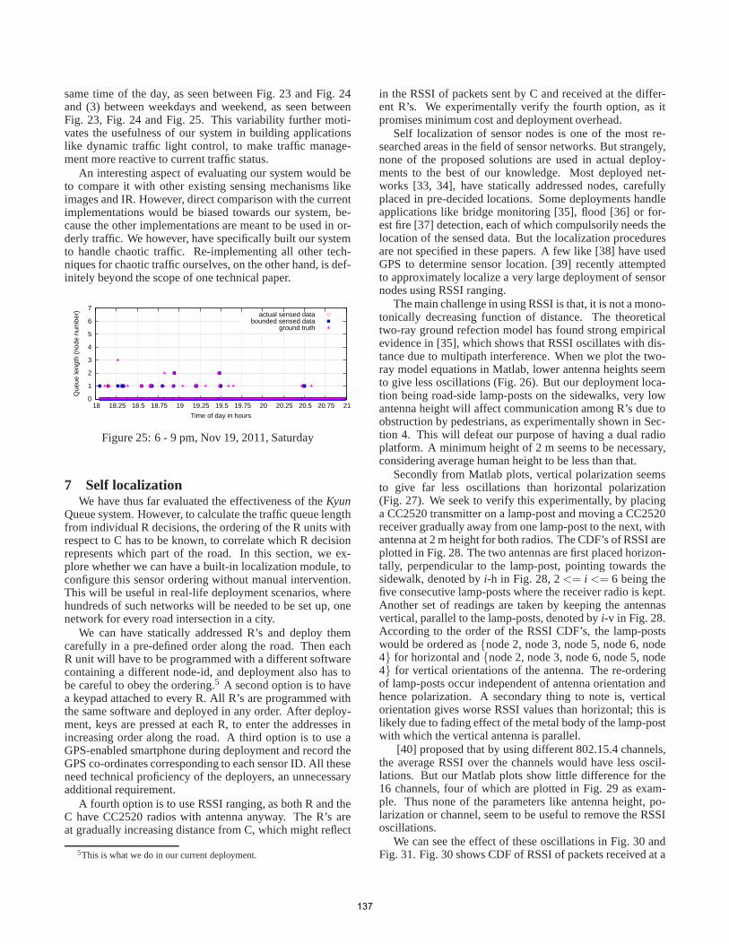
same time of the day, as seen between Fig. 23 and Fig. 24and (3) between weekdays and weekend, as seen betweenFig. 23, Fig. 24 and Fig. 25. This variability further moti-vates the usefulness of our system in building applicationslike dynamic traffic light control, to make traffic manage-ment more reactive to current traffic status.

An interesting aspect of evaluating our system would beto compare it with other existing sensing mechanisms likeimages and IR. However, direct comparison with the currentimplementations would be biased towards our system, be-cause the other implementations are meant to be used in or-derly traffic. We however, have specifically built our systemto handle chaotic traffic. Re-implementing all other tech-niques for chaotic traffic ourselves, on the other hand, is def-initely beyond the scope of one technical paper.

0

1

2

3

4

5

6

7

18 18.25 18.5 18.75 19 19.25 19.5 19.75 20 20.25 20.5 20.75 21

Que

ue le

ngth

(no

de n

umbe

r)



ground truth


7 Self localizationWe have thus far evaluated the effectiveness of theKyun

Queue system. However, to calculate the traffic queue lengthfrom individual R decisions, the ordering of the R units withrespect to C has to be known, to correlate which R decisionrepresents which part of the road. In this section, we ex-plore whether we can have a built-in localization module, toconfigure this sensor ordering without manual intervention.This will be useful in real-life deployment scenarios, wherehundreds of such networks will be needed to be set up, onenetwork for every road intersection in a city.

We can have statically addressed R’s and deploy themcarefully in a pre-defined order along the road. Then eachR unit will have to be programmed with a different softwarecontaining a different node-id, and deployment also has tobe careful to obey the ordering.5 A second option is to havea keypad attached to every R. All R’s are programmed withthe same software and deployed in any order. After deploy-ment, keys are pressed at each R, to enter the addresses inincreasing order along the road. A third option is to use aGPS-enabled smartphone during deployment and record theGPS co-ordinates corresponding to each sensor ID. All theseneed technical proficiency of the deployers, an unnecessaryadditional requirement.

A fourth option is to use RSSI ranging, as both R and theC have CC2520 radios with antenna anyway. The R’s areat gradually increasing distance from C, which might reflect

5This is what we do in our current deployment.

in the RSSI of packets sent by C and received at the differ-ent R’s. We experimentally verify the fourth option, as itpromises minimum cost and deployment overhead.

Self localization of sensor nodes is one of the most re-searched areas in the field of sensor networks. But strangely,none of the proposed solutions are used in actual deploy-ments to the best of our knowledge. Most deployed net-works [33, 34], have statically addressed nodes, carefullyplaced in pre-decided locations. Some deployments handleapplications like bridge monitoring [35], flood [36] or for-est fire [37] detection, each of which compulsorily needs thelocation of the sensed data. But the localization proceduresare not specified in these papers. A few like [38] have usedGPS to determine sensor location. [39] recently attemptedto approximately localize a very large deployment of sensornodes using RSSI ranging.

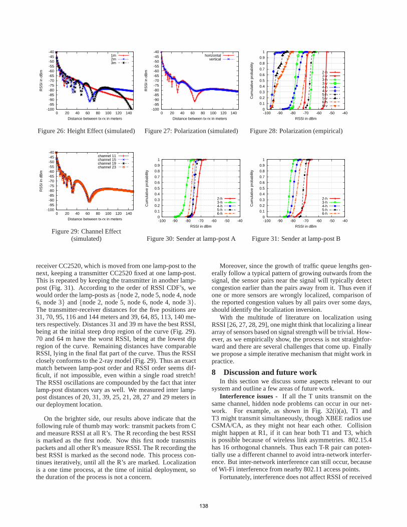
The main challenge in using RSSI is that, it is not a mono-tonically decreasing function of distance. The theoreticaltwo-ray ground refection model has found strong empiricalevidence in [35], which shows that RSSI oscillates with dis-tance due to multipath interference. When we plot the two-ray model equations in Matlab, lower antenna heights seemto give less oscillations (Fig. 26). But our deployment loca-tion being road-side lamp-posts on the sidewalks, very lowantenna height will affect communication among R’s due toobstruction by pedestrians, as experimentally shown in Sec-tion 4. This will defeat our purpose of having a dual radioplatform. A minimum height of 2 m seems to be necessary,considering average human height to be less than that.

Secondly from Matlab plots, vertical polarization seemsto give far less oscillations than horizontal polarization(Fig. 27). We seek to verify this experimentally, by placinga CC2520 transmitter on a lamp-post and moving a CC2520receiver gradually away from one lamp-post to the next, withantenna at 2 m height for both radios. The CDF’s of RSSI areplotted in Fig. 28. The two antennas are first placed horizon-tally, perpendicular to the lamp-post, pointing towards thesidewalk, denoted byi-h in Fig. 28, 2<= i <= 6 being thefive consecutive lamp-posts where the receiver radio is kept.Another set of readings are taken by keeping the antennasvertical, parallel to the lamp-posts, denoted byi-v in Fig. 28.According to the order of the RSSI CDF’s, the lamp-postswould be ordered as{node 2, node 3, node 5, node 6, node4} for horizontal and{node 2, node 3, node 6, node 5, node4} for vertical orientations of the antenna. The re-orderingof lamp-posts occur independent of antenna orientation andhence polarization. A secondary thing to note is, verticalorientation gives worse RSSI values than horizontal; this islikely due to fading effect of the metal body of the lamp-postwith which the vertical antenna is parallel.

[40] proposed that by using different 802.15.4 channels,the average RSSI over the channels would have less oscil-lations. But our Matlab plots show little difference for the16 channels, four of which are plotted in Fig. 29 as exam-ple. Thus none of the parameters like antenna height, po-larization or channel, seem to be useful to remove the RSSIoscillations.

We can see the effect of these oscillations in Fig. 30 andFig. 31. Fig. 30 shows CDF of RSSI of packets received at a

137

-100-95-90-85-80-75-70-65-60-55-50-45-40

0 20 40 60 80 100 120 140

RS

SI i

n dB

m

Distance between tx-rx in meters

1m2m3m

Figure 26: Height Effect (simulated)

-100-95-90-85-80-75-70-65-60-55-50-45-40

0 20 40 60 80 100 120 140

RS

SI i

n dB

m


horizontalvertical

Figure 27: Polarization (simulated)

0

0.1

0.2

0.3

0.4

0.5

0.6

0.7

0.8

0.9

1

-100 -90 -80 -70 -60 -50 -40

Cum

ulat

ive

prob

abili

ty

RSSI in dBm

2-h2-v3-h3-v4-h4-v5-h5-v6-h6-v

Figure 28: Polarization (empirical)

-100-95-90-85-80-75-70-65-60-55-50-45-40

0 20 40 60 80 100 120 140

RS

SI i

n dB

m


channel 11channel 15channel 19channel 23

Figure 29: Channel Effect(simulated)

0

0.1

0.2

0.3

0.4

0.5

0.6

0.7

0.8

0.9

1

-100 -90 -80 -70 -60 -50 -40

Cum

ulat

ive

prob

abili

ty

RSSI in dBm

2-h3-h4-h5-h6-h

Figure 30: Sender at lamp-post A

0

0.1

0.2

0.3

0.4

0.5

0.6

0.7

0.8

0.9

1

-100 -90 -80 -70 -60 -50 -40

Cum

ulat

ive

prob

abili

ty

RSSI in dBm

2-h3-h4-h5-h6-h

Figure 31: Sender at lamp-post B

receiver CC2520, which is moved from one lamp-post to thenext, keeping a transmitter CC2520 fixed at one lamp-post.This is repeated by keeping the transmitter in another lamp-post (Fig. 31). According to the order of RSSI CDF’s, wewould order the lamp-posts as{node 2, node 5, node 4, node6, node 3} and{node 2, node 5, node 6, node 4, node 3}.The transmitter-receiver distances for the five positions are31, 70, 95, 116 and 144 meters and 39, 64, 85, 113, 140 me-ters respectively. Distances 31 and 39 m have the best RSSI,being at the initial steep drop region of the curve (Fig. 29).70 and 64 m have the worst RSSI, being at the lowest dipregion of the curve. Remaining distances have comparableRSSI, lying in the final flat part of the curve. Thus the RSSIclosely conforms to the 2-ray model (Fig. 29). Thus an exactmatch between lamp-post order and RSSI order seems dif-ficult, if not impossible, even within a single road stretch!The RSSI oscillations are compounded by the fact that interlamp-post distances vary as well. We measured inter lamp-post distances of 20, 31, 39, 25, 21, 28, 27 and 29 meters inour deployment location.

On the brighter side, our results above indicate that thefollowing rule of thumb may work: transmit packets from Cand measure RSSI at all R’s. The R recording the best RSSIis marked as the first node. Now this first node transmitspackets and all other R’s measure RSSI. The R recording thebest RSSI is marked as the second node. This process con-tinues iteratively, until all the R’s are marked. Localizationis a one time process, at the time of initial deployment, sothe duration of the process is not a concern.

Moreover, since the growth of traffic queue lengths gen-erally follow a typical pattern of growing outwards from thesignal, the sensor pairs near the signal will typically detectcongestion earlier than the pairs away from it. Thus even ifone or more sensors are wrongly localized, comparison ofthe reported congestion values by all pairs over some days,should identify the localization inversion.

With the multitude of literature on localization usingRSSI [26, 27, 28, 29], one might think that localizing a lineararray of sensors based on signal strength will be trivial. How-ever, as we empirically show, the process is not straightfor-ward and there are several challenges that come up. Finallywe propose a simple iterative mechanism that might work inpractice.

8 Discussion and future workIn this section we discuss some aspects relevant to our

system and outline a few areas of future work.Interference issues - If all the T units transmit on the

same channel, hidden node problems can occur in our net-work. For example, as shown in Fig. 32(i)(a), T1 andT3 might transmit simultaneously, though XBEE radios useCSMA/CA, as they might not hear each other. Collisionmight happen at R1, if it can hear both T1 and T3, whichis possible because of wireless link asymmetries. 802.15.4has 16 orthogonal channels. Thus each T-R pair can poten-tially use a different channel to avoid intra-network interfer-ence. But inter-network interference can still occur, becauseof Wi-Fi interference from nearby 802.11 access points.

Fortunately, interference does not affect RSSI of received

138

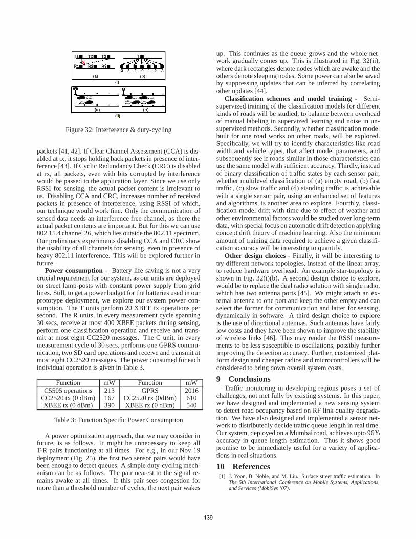
Figure 32: Interference & duty-cycling

packets [41, 42]. If Clear Channel Assessment (CCA) is dis-abled at tx, it stops holding back packets in presence of inter-ference [43]. If Cyclic Redundancy Check (CRC) is disabledat rx, all packets, even with bits corrupted by interferencewould be passed to the application layer. Since we use onlyRSSI for sensing, the actual packet content is irrelevant tous. Disabling CCA and CRC, increases number of receivedpackets in presence of interference, using RSSI of which,our technique would work fine. Only the communication ofsensed data needs an interference free channel, as there theactual packet contents are important. But for this we can use802.15.4 channel 26, which lies outside the 802.11 spectrum.Our preliminary experiments disabling CCA and CRC showthe usability of all channels for sensing, even in presence ofheavy 802.11 interference. This will be explored further infuture.

Power consumption - Battery life saving is not a verycrucial requirement for our system, as our units are deployedon street lamp-posts with constant power supply from gridlines. Still, to get a power budget for the batteries used in ourprototype deployment, we explore our system power con-sumption. The T units perform 20 XBEE tx operations persecond. The R units, in every measurement cycle spanning30 secs, receive at most 400 XBEE packets during sensing,perform one classification operation and receive and trans-mit at most eight CC2520 messages. The C unit, in everymeasurement cycle of 30 secs, performs one GPRS commu-nication, two SD card operations and receive and transmit atmost eight CC2520 messages. The power consumed for eachindividual operation is given in Table 3.

Function mW Function mWC5505 operations 213 GPRS 2016

CC2520 tx (0 dBm) 167 CC2520 rx (0dBm) 610XBEE tx (0 dBm) 390 XBEE rx (0 dBm) 540

Table 3: Function Specific Power Consumption

A power optimization approach, that we may consider infuture, is as follows. It might be unnecessary to keep allT-R pairs functioning at all times. For e.g., in our Nov 19deployment (Fig. 25), the first two sensor pairs would havebeen enough to detect queues. A simple duty-cycling mech-anism can be as follows. The pair nearest to the signal re-mains awake at all times. If this pair sees congestion formore than a threshold number of cycles, the next pair wakes

up. This continues as the queue grows and the whole net-work gradually comes up. This is illustrated in Fig. 32(ii),where dark rectangles denote nodes which are awake and theothers denote sleeping nodes. Some power can also be savedby suppressing updates that can be inferred by correlatingother updates [44].

Classification schemes and model training - Semi-supervized training of the classification models for differentkinds of roads will be studied, to balance between overheadof manual labeling in supervized learning and noise in un-supervized methods. Secondly, whether classification modelbuilt for one road works on other roads, will be explored.Specifically, we will try to identify characteristics like roadwidth and vehicle types, that affect model parameters, andsubsequently see if roads similar in those characteristics canuse the same model with sufficient accuracy. Thirdly, insteadof binary classification of traffic states by each sensor pair,whether multilevel classification of (a) empty road, (b) fasttraffic, (c) slow traffic and (d) standing traffic is achievablewith a single sensor pair, using an enhanced set of featuresand algorithms, is another area to explore. Fourthly, classi-fication model drift with time due to effect of weather andother environmental factors would be studied over long-termdata, with special focus on automatic drift detection applyingconcept drift theory of machine learning. Also the minimumamount of training data required to achieve a given classifi-cation accuracy will be interesting to quantify.

Other design choices -Finally, it will be interesting totry different network topologies, instead of the linear array,to reduce hardware overhead. An example star-topology isshown in Fig. 32(i)(b). A second design choice to explore,would be to replace the dual radio solution with single radio,which has two antenna ports [45]. We might attach an ex-ternal antenna to one port and keep the other empty and canselect the former for communication and latter for sensing,dynamically in software. A third design choice to exploreis the use of directional antennas. Such antennas have fairlylow costs and they have been shown to improve the stabilityof wireless links [46]. This may render the RSSI measure-ments to be less susceptible to oscillations, possibly furtherimproving the detection accuracy. Further, customized plat-form design and cheaper radios and microcontrollers will beconsidered to bring down overall system costs.

9 ConclusionsTraffic monitoring in developing regions poses a set of

challenges, not met fully by existing systems. In this paper,we have designed and implemented a new sensing systemto detect road occupancy based on RF link quality degrada-tion. We have also designed and implemented a sensor net-work to distributedly decide traffic queue length in real time.Our system, deployed on a Mumbai road, achieves upto 96%accuracy in queue length estimation. Thus it shows goodpromise to be immediately useful for a variety of applica-tions in real situations.

10 References[1] J. Yoon, B. Noble, and M. Liu. Surface street traffic estimation. In

The 5th International Conference on Mobile Systems, Applications,and Services (MobiSys ’07).

139

[2] E.Koukoumidis, L.Peh, and M.Martonosi. Signalguru: Leveragingmobile phones for collaborative traffic signal schedule advisory. InThe 9th International Conference on Mobile Systems, Applications,and Services (MobiSys ’11).

[3] R. Sen, P. Siriah, and B. Raman. Roadsoundsense: Acoustic sensingbased road congestion monitoring in developing regions. InThe 8thAnnual IEEE Communications Society Conference on Sensor, Meshand Ad Hoc Communications and Networks (SECON ’11).

[4] www.pluggd.in/indian-traffic-entrepreneurial-lessons-297/ .[5] B. Coifman and M. Cassidy. Vehicle reidentification and travel time

measurement on congested freeways.Transportation Research PartA: Policy and Practice, 36(10):899–917, 2002.

[6] http://www.scats.com.au/index.html .[7] http://paleale.eecs.berkeley.edu/ ˜ varaiya/transp.html .[8] http://www.visioway.com,http://www.traficon.com .[9] http://www.mapunity.in/ .

[10] http://www.ceos.com.au/products/tirtl.htm .[11] I. Magrini G. Manes A. Manes B. Barbagli, L. Bencini. An end to

end wsn based system for real-time traffic monitoring. InThe 8thEuropean Conference on Wireless Sensor Networks (EWSN ’11).

[12] R. Sen, B. Raman, and P. Sharma. Horn-ok-please. InThe 8th Inter-national Conference on Mobile Systems, Applications, and Services(MobiSys ’10).

[13] http://traffic.berkeley.edu/theproject.html .[14] A. Thiagarajan, L. Ravindranath, K. LaCurts, S. Madden, H. Balakr-

ishnan, S. Toledo, and J. Eriksson. Vtrack: Accurate, energy-awareroad traffic delay estimation using mobile phones. InThe 7th ACMConference on Embedded Networked Sensor Systems (SenSys ’09).

[15] R.Balan, N.Khoa, and J.Lingxiao. Real-time trip information servicefor a large taxi fleet. InThe 9th International Conference on MobileSystems, Applications, and Services (MobiSys ’11).

[16] P. Mohan, V. N. Padmanabhan, and R. Ramjee. Nericell: rich mon-itoring of road and traffic conditions using mobile smartphones. InThe 10th ACM Conference on Embedded Networked Sensor Systems(SenSys ’08).

[17] V. Kastrinaki, M. Zervakis, and K. Kalaitzakis. A survey of videoprocessing techniques for traffic applications.Image and Vision Com-puting, 2003.

[18] A. Quinn and R. Nakibuule. Traffic flow monitoring in crowded cities.In AAAI Spring Symposium on Artificial Intelligence for Development,2010.

[19] V. Jain, A. Sharma, and L. Subramanian. Road traffic congestion inthe developing world. InThe 2nd Annual Symposium on Computingfor Development (DEV ’12).

[20] Skordylis A. and Trigoni N. Efficient data propagation in traffic-monitoring vehicular networks.IEEE Transactions on ITS, volume12, 2011.

[21] Leontiadis I., Marfia G., Mack D., Pau G., Mascolo C., and Gerla M.On the effectiveness of an opportunistic traffic management systemfor vehicular networks.IEEE Transactions on ITS, volume 12, issue4, 2011.

[22] Skordylis A. and Trigoni N. Delay-bounded routing in vehicular ad-hoc networks. Inthe 9th International Symposium on Mobile Ad HocNetworking and Computing (MobiHoc ’08).

[23] Yuan J., Zheng Y., Xie X, and Sun G. T-drive: Enhancing driving di-rections with taxi drivers intelligence. InTransactions on Knowledgeand Data Engineering (TKDE ’12).

[24] H. K. Le, J. Pasternack, H. Ahmadi, M. Gupta, Y. Sun, T. Abdelzaher,J. Han, D. Roth, B. K. Szymanski, and S. Adali. Apollo: Towardsfactfinding in participatory sensing. InThe 10th ACM/IEEE Confer-ence on Information Processing in Sensor Networks (IPSN ’11).

[25] V. Shrivastava, D. Agrawal, A. Mishra, and S. Banerjee. Understand-ing the limitations of transmit power control for indoor wlans. InThe7th Internet Measurement Conference (IMC ’07).

[26] Moustafa Y. and Agrawala A. The horus wlan location determina-tion system. InThe 3rd International Conference on Mobile Systems,Applications, and Services (MobiSys ’05).

[27] Chintalapudi K., Iyer A. P., and Padmanabhan V. N. Indoor localiza-tion without the pain. InThe 16th Annual International Conferenceon Mobile Computing and Networking (MobiCom ’10).

[28] Patwari N. and Wilson J. Rf sensor networks for device-free localiza-tion: Measurements, models, and algorithms. InProceedings of theIEEE, volume 98, number 11, 2010.

[29] Xu C., Firner B., Zhang Y., Howard R., and J. Li. Statistical learn-ing strategies for rf-based indoor device-free passive localization. InThe 9th ACM Conference on Embedded Networked Sensor Systems(SenSys ’11).

[30] Mottola L., Picco G. P., Ceriotti M., Guna S., and Murphy A. L. Notall wireless sensor networks are created equal: A comparative studyon tunnels. InACM Transactions on Sensor Networks (TOSN ’10).

[31] Anonymous picasa album containing ground truth images and sam-ple videos from deployment location. Inhttps://picasaweb.google.com/108285005574366399467.

[32] V. Gabale, B. Raman, K. Chebrolu, and P. Kulkarni. Lit mac: Address-ing the challenges of effective voice communication in a low cost, lowpower wireless mesh network. InThe 1st Annual Symposium on Com-puting for Development (DEV ’10).

[33] T. He, S. Krishnamurthy, J. Stankovic, T. Abdelzaher, L. Luo,R. Stoleru, T. Yan, L. Gu, J. Hui, and B. Krogh. Energy-efficientsurveillance system using wireless sensor networks. InThe 2nd Inter-national Conference on Mobile Systems, Applications, and Services(MobiSys ’04).

[34] X. Jiang, M. Van Ly, J. Taneja, P. Dutta, and D. Culler. Experienceswith a high-fidelity wireless building energy auditing network. InThe7th ACM Conference on Embedded Networked Sensor Systems (Sen-Sys ’09).

[35] K. Chebrolu, B. Raman, N. Mishra, P. Valiveti, and R. Kumar. Bri-mon: a sensor network system for railway bridge monitoring. InThe6th International Conference on Mobile Systems, Applications, andServices (MobiSys ’08).

[36] E. Basha, S. Ravela, and D. Rus. Model-based monitoring for earlywarning flood detection. InThe 6th ACM Conference on EmbeddedNetworked Sensor Systems (SenSys ’08).

[37] C. Hartung, R. Han, C. Seielstad, and S. Holbrook. Firewxnet: amulti-tiered portable wireless system for monitoring weather condi-tions in wildland fire environments. InThe 4th International Confer-ence on Mobile Systems, Applications, and Services (MobiSys ’06).

[38] W. Song, R. Huang, M. Xu, A. Ma, B. Shirazi, and R. LaHusen. Air-dropped sensor network for real-time high-fidelity volcano monitor-ing. InThe 7th International Conference on Mobile Systems, Applica-tions, and Services (MobiSys ’09).

[39] W. Xi, Y. He, Y. Liu, J. Zhao, L. Mo, Z. Yang, J. Wang, and X. Li.Locating sensors in the wild: pursuit of ranging quality. InThe 8thACM Conference on Embedded Networked Sensor Systems (SenSys’10).

[40] A. Bardella, N. Bui, A. Zanella, M. Zorzi, P. Marron, T. Voigt,P. Corke, and L. Mottola. An experimental study on ieee 802.15.4multichannel transmission to improve rssibased service performance.In The 5th Workshop on Real-World Wireless Sensor Networks (RE-ALWSN ’10).

[41] S. Rayanchu, A. Mishra, D. Agrawal, S. Saha, and S. Banerjee. Di-agnosing wireless packet losses in 802.11: Separating collision fromweak signal. InThe 27th IEEE International Conference on ComputerCommunications (INFOCOM ’08).

[42] J. Hauer, V. Handziski, and A. Wolisz. Experimental study of theimpact of wlan interference on ieee 802.15.4 body area networks. InThe 6th European Conference on Wireless Sensor Networks (EWSN’09).

[43] C. Mike Liang, N. B. Priyantha, J. Liu, and A. Terzis. Surviving wi-fiinterference in low power zigbee networks. InThe 10th ACM Confer-ence on Embedded Networked Sensor Systems (SenSys ’10).

[44] Guitton A., Skordylis A., and Trigoni N. Utilizing correlations tocompress time-series in traffic monitoring sensor networks. InIEEEWireless Communications and Networking Conference (WCNC ’07).

[45] http://www.jennic.com/products/modules/jn5148_modules,http://www.jennic.com/products/modules/jn5139_modules .

[46] Ostrom E., Mottola L., and Voigt T. Evaluation of an electronicallyswitched directional antenna for real-world low-power wireless net-works. InThe 5th Workshop on Real-World Wireless Sensor Networks(REALWSN ’10).

140

Documents

Kyun Queue: A Sensor Network System To Monitor Road …