L1-consistent adaptive multivariate histogramsfrom a randomized queue prioritized for

statistically equivalent blocksUCDMS Research Report 2014/2 (Thu Oct 23 02:02:47 EDT 2014, Ithaca, NY)

Gloria Teng1, Jennifer Harlow2, and Raazesh Sainudiin2

1 Universiti Tunku Abdul Rahman, Kuala Lumpur 53300, Malaysiagloriateng@utar.edu.my

2 University of Canterbury, Christchurch 8041, New Zealandjenny.harlow@canterbury.ac.nzraazesh.sainudiin@gmail.com

Abstract. An L1-consistent data-adaptive histogram estimator driven by a random-ized queue prioritized by a statistically equivalent blocks rule is obtained. Such data-dependent histograms are formalized as real mapped regular pavings (R-MRP). Aregular paving (RP) is a binary tree obtained by selectively bisecting boxes alongtheir first widest side. A statistical regular paving (SRP) augments an RP by muta-bly caching the recursively computable sufficient statistics of the data. Mapping a realvalue to each element of the partition gives an R-MRP that can be used to represent apiecewise-constant function density estimate on a multidimensional domain. R-MRPsare closed under addition and allow for efficient averaging of histograms with differentpartitions in any dimension. A partitioning strategy driven by a randomized priorityqueue of the current leaf nodes of an SRP is formalized as a Markov chain over thespace of SRPs and the conditions for its L1-consistency are obtained.

1 Introduction

Suppose our random variable X has an unknown density f on Rd, then for allBorel sets A ⊆ Rd,

µ(A) := Pr{X ∈ A} =∫A

f(x)dx .

Any density estimate fn(x) = fn(x;X1, X2, . . . , Xn) : Rd ×(Rd)n → R, is

simply a map from(Rd)n+1 to R. The objective in density estimation is to es-

timate the unknown f from an independent and identically distributed sampleX1, X2, . . . , Xn drawn from f . This density estimate fn of the unknown f givesus a means of computing the probabilities of any Borel set A ∈ Bd or of com-puting the density at any point x ∈ Rd. Density estimation is often the firststep in many learning tasks, including, classification, regression and clustering.

There are two general approaches to density estimation: parametric densityestimation and nonparametric density estimation. Here we are concerned with

nonparametric density estimation. Histograms and kernel density estimates arethe two most common forms of nonparametric density estimate for data assumedto be drawn from a continuous distribution. Both can be used for univariate andmultivariate data. Other density estimators include orthogonal series estimatorsand nearest neighbour estimators [16, chap. 2]. Adaptations and specializationsof these density estimation methods may be used for particular types of data,high-dimensional data, and very large data sets [15, 8]. However it is formed,the density estimate is some smoothed representation of the observed data [18].The density estimation method determines how this smoothing is performed.Data-adaptive density estimation methods adapt the amount of smoothing tothe local density of the data [16, chap. 2].

For a given prior distribution over SRPs, the posterior mean can be thoughtof as an L2-loss minimizing Bayesian nonparametric density estimate. Such aBayesian smoothing based on the sample mean of a sequence of histogram statesvisited by an MCMC algorithm with stationary samples from the posterior dis-tribution was given in [12]. The crucial strategy to initialize the MCMC chainfrom states with high posterior probability, in order to minimize the chance thatthe chain gets stuck in low posterior states, was done in a an ad hoc manner in[12]. This paper proposes the use of an L1-consistent and data-dependent tree-based histogram, that is built using a data structure known as statistical regularpaving (SRP), as an initializing strategy for the MCMC in [12]. SRP is an exten-sion of a regular paving (RP) [13, 6, 5], a class of space-partitioning trees thatcan facilitate efficient arithmetical operations. A real mapped regular paving(R-MRP) is an extension of an RP designed to represent a piecewise-constantfunction and allow efficient arithmetical operations with them, including the av-eraging of R-MRP histogram states with different partitions that are visited byan MCMC algorithm as in [12]. An SRP augments an RP by mutably cachingrecursively computable sufficient statistics of the data. A histogram density es-timate represented as an R-MRP can then be created from an SRP. Moreover,such histogram density estimates allow for a wide range of subsequent statisti-cal operations, such as, creating marginal and conditional density estimates orevaluating the density estimate at a large set of query points, to be performedefficiently [5].

The paper is laid out as follows. Section 2 reviews various tree-based his-togram estimators in the literature. Section 3 introduces the arithmetic andalgebra for RPs, R-MRPs, and SRPs, and explains how a histogram can bebuilt using these structures. Section 4 illustrates the use of a randomized pri-ority queue to partition the histogram and a proof of the L1-consistency of thisadaptive partitioning scheme. Section 5 concludes.

2 Tree-based histograms

A histogram is based on a partition of the data space; the elements of the parti-tion are commonly known as bins. The choice of bin width(s) is the smoothingproblem: wider bins give more smoothing, narrower bins less smoothing. Thebins of a regular histogram are all equally-sized; the bins of an irregular his-togram can vary in size.

Regular partitioning with small enough bins to suit the modes of the densitywill give too many bins in low or flat density areas [11]. Regular partitioningwith a bin width more suited to the overall variability of the data may com-promise the potential of the histogram to show important local features in thehighest density areas. Multivariate histograms with a single bin width are notable to adapt to spatially varying smoothing requirements [7, chap. 17]. A data-dependent partition allows the bin width to vary in a way that is determinedby the data. Data-dependent partitions can provide estimates which are theo-retically superior to those using partitions based simply on the number of datapoints in the data set [17], and under certain conditions, a histogram densityestimate with a data-dependent partition can be strongly L1-consistent [9].

A tree structure can be used in algorithms for creating data-adaptive his-tograms. This is especially suitable where the algorithm uses some form ofrecursive partitioning strategy, often in association with a penalty function tocontrol complexity. A greedy partitioning algorithm makes locally optimal deci-sions (with respect to the chosen optimality criterion) based on the immediatelyavailable information in each step but is not guaranteed to find a globally opti-mal solution. Several greedy data-adaptive tree-structured histogram algorithmshave been developed, including methods that grow the tree (partition) step-by-step or that grow the tree to represent the most complex allowable partitionand then use a greedy algorithm to prune to reduce the tree (reduce the numberof elements in the partition. Partitioning trees can also be used in non-greedycomplexity-penalized optimization algorithms that perform an exhaustive com-parison of a limited set of possible partitions. For a discussion of such tree-basedapproaches see [7, chap. 17 & 18] and the references therein.

In general, computational efficiency of the methods described above sufferin two basic ways. First, they are not well-suited to very high-dimensional databecause the computational complexity of most density estimation algorithmsgrows exponentially with the dimensions [14, chap. 7], irrespective of the com-plexity of the underlying density. Second, these methods cannot cope with largevolumes of data, say with sample size n around 105 or 106, even in small dimen-sions, say dimension d up to 4 or 5. A Metropolis-Hastings Markov chain methodwas developed in [12] with stationary distribution given by a posterior distribu-tion over regular paving histograms and used to estimate the posterior expecta-tion by exploiting the arithmetic properties of regular pavings when averaging

histogram samples from the chain. The averaged regular paving histogram den-sity estimate was tested with uniform data in up to d = 1, 000 dimensions andfound that the method coped well with this type of high-dimensional unstruc-tured data. Results using data simulated from uniform mixture approximationsto non-uniform structured densities such as multivariate Gaussian and Rosen-brock densities showed that the number of dimensions in which the methodis computationally feasible with reasonably smaller mean integrated absoluteerrors is much lower, about d = 5 or d = 6. However, the method can com-putationally cope with large volumes of data, even n as high as 107, in starkcontrast with other available methods.

Many conventional kernel density estimation methods are only effective withdata in less than five or six dimensions [3, 19] with sample sizes around fewthousands and generally reach computational bottle-necks when the samplesize reaches 104. The posterior histogram estimate of [12] therefore has someattractions as a density estimation method in up to around five dimensions es-pecially in situations where there is a large amount of sample data availableand where it is advantageous to be able to carry out subsequent statisticaloperations efficiently, directly on the density estimate itself. Such statistical op-erations include (i) evaluating of the density over a large set of query points forcross-validation, (ii) obtaining the highest density or coverage regions, (iii) get-ting marginal densities as R-MRPs by tree-based integration over a subset of thecoordinates, or (iv) producing conditional densities as R-MRPs for subsequentregression, according to the algorithms in [5].

3 Regular pavings and histograms

This section introduces the notions of RPs, SRPs, and R-MRPs, and explainshow a histogram density estimate can be built using these data structures.

3.1 Regular pavings (RPs)

Let x := [x, x] be a compact real interval with lower bound x and upper boundx, where x ≤ x. Let the space of such intervals be IR. The width of an interval xis wid (x) := x− x. The midpoint is mid (x) := (x+ x) /2. A box of dimensiond with coordinates in ∆ := {1, 2, . . . , d} is an interval vector:

x := [x1, x1]× . . .× [xd, xd] =: �j∈∆

[xj, xj] .

The set of all such boxes is IRd, i.e., the set of all interval real vectors in dimen-sion d. Consider a box x in IRd. Define the index ι to be the first coordinate ofmaximum width:

ι := min

(argmax

i(wid (xi))

).

A bisection or split of x perpendicularly at the mid-point along this first widestcoordinate ι gives the left and right child boxes of x

xL := [x1, x1]× . . .× [xι,mid (xι))× [xι+1, xι+1]× . . .× [xd, xd] ,

xR := [x1, x1]× . . .× [mid (xι), xι]× [xι+1, xι+1]× . . .× [xd, xd] .

Such a bisection is said to be regular. Note that this bisection gives the left childbox a half-open interval [xι,mid (xι)) on coordinate ι so that the intersectionof the left and right child boxes is empty.

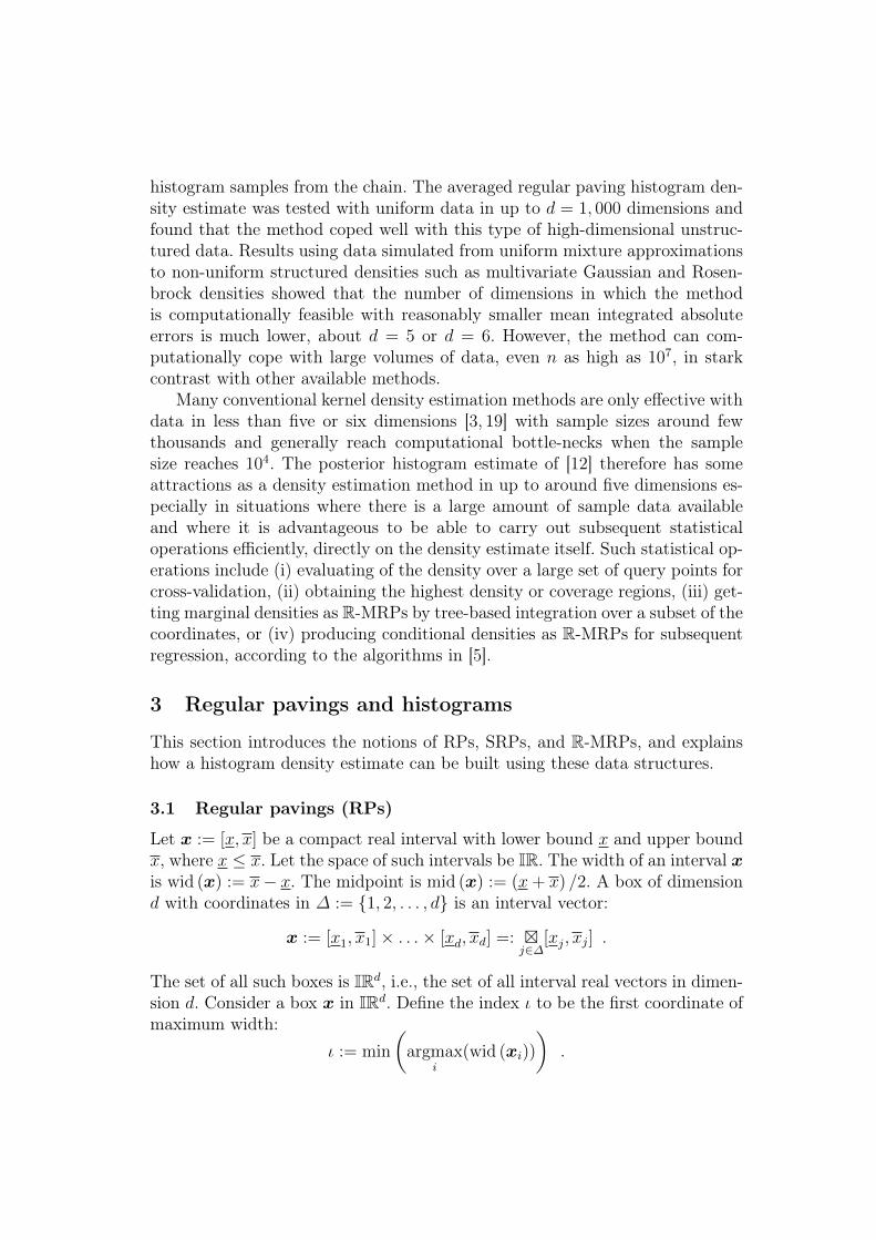
A recursive sequence of selective regular bisections of boxes, with possiblyopen boundaries, along the first widest coordinate, starting from the root boxx in IRd is known as a regular paving [6] or n-tree [13] of x. A regular pavingof x can also be seen as a binary tree formed by recursively bisecting the boxx at the root node. Each node in the binary tree has either no children or twochildren. When the root box x is clear from the context we refer to an RP ofx as merely an RP. Each node of an RP is associated with a sub-box of theroot box that can be attained by a sequence of selective regular bisections. Eachnode in an RP can be distinctly labelled by the sequence of child node selectionsfrom the root node. We label these nodes and the associated boxes with stringscomposed of L and R for left and right, respectively. For example, in Figure 1,the root node associated with root box xρ is labeled ρ.

The relationship of trees, labels and partitions is illustrated in Figure 1 usinga simple one-dimensional example. The root node associated with root intervalxρ ∈ IR is labelled ρ. First, ρ is split into two child nodes, and the left child andright child nodes are labelled ρL and ρR, respectively. The left half of xρ that isnow associated with node ρL is labelled xρL. Similarly, the right half of xρ thatis associated with the right child node ρR is labelled xρR. ρL and ρR are a pairof sibling nodes since they share the same parent node ρ. A node with no childnodes is called a leaf node. A cherry node is a sub-terminal node with a pair ofchild nodes that are both leaves. This pair of sibling nodes can be reunited ormerged to its parent cherry node ρ, thereby turning the cherry node into a leafnode.

Returning to Figure 1, the left node ρL is split to get its left and right childnodes ρLL and ρLR with associated sub-intervals xρLL and xρLR respectively,formed by the bisection of interval xρL (because the root interval xρ is one-dimensional, each bisection is always on that single coordinate).

Let the j-th interval of a box xρv be [xρv,j, xρv,j]. The volume of a d-dimensionalbox xρv associated with the node ρv of an RP of xρ is the product of the side-lengths of the box, that is, vol (xρv) =

∏dj=1(xρv,j − xρv,j).

The volume is associated with the depth of a node. The depth of a node ρvin an RP is denoted by dρv. A node has depth dρv = k in the tree if it can bereached by k splits from the root node. If an RP has root box xρ and a node ρv in

Fig. 1. A sequence of selective bisections, starting from the root, produces an RP.

the regular paving has depth k, then the volume of the box xρv associated withthat node is vol (xρv) = 2−kvol (xρ). This is because any split always results inthe child node’s box having half the volume of the parent node’s box.

In general, an RP is denoted by s. The set of all nodes of an RP is denotedby V := ρ ∪ {ρ{L,R}j : j ∈ N}. The set of all leaf nodes of an RP is denotedby L. The boxes associated with the leaf nodes of an RP are the partition ofthe root box xρ. The set of leaf boxes of a regular paving s with root box xρ isdenoted by xL(s). Let Sk be the set of all regular pavings with root box xρ madeof k splits. Note that the number of leaf nodes m = |L(s)| = k + 1 if s ∈ Sk.

The number of distinct binary trees with k splits is equal to the Catalannumber Ck.

Ck =1

k + 1

(2k

k

)=

(2k)!

(k + 1)!(k!). (1)

For i, j ∈ Z+, where Z+ := {0, 1, 2, . . .} and i ≤ j, let Si:j be the set of regularpavings with k splits where k ∈ {i, i+1, . . . , j}. The space of all regular pavingsis then S0:∞ := limj→∞ S0:j. The size of the space of all regular pavings withbetween i and j splits, |Si:j|, is given by the sum of Catalan numbers:

|Si:j| =j∑k=i

Ck . (2)

The size of the space of all regular pavings with up to k splits is |S0:k|.

3.2 Real mapped regular pavings (R-MRPs)

A real mapped regular paving (R-MRP) is an extension of an RP. Let s ∈ S0:∞be an RP with root node ρ and root box xρ ∈ IRd. Let �f : V(s) → R mapeach node of s to an element in R as follows:

{ρv 7→ fρv : ρv ∈ V(s), fρv ∈ R} .

Such a map �f is called an R-mapped regular paving (R-MRP). Thus, an R-MRP �f is obtained by augmenting each node ρv of the RP tree s with anadditional data member fρv ∈ R.

The sets of all nodes and leaf nodes of an R-MRP �f are denoted by V( �f)and L( �f), respectively. The set of all leaf node boxes is denoted by xL(�f). Theclass of R-MRPs over the leaf boxes of regular pavings of a root box xρ ∈ IRd

is then�F := {{ρv 7→ fρv : ρv ∈ V(s), fρv ∈ R} : s ∈ S0:∞}

Arithmetic operations in R can be extended to R-MRPs [5]. For example,given any two R-MRPs �f (1) and �f (2) with the same root box xρ and a binaryoperation ? ∈ {+,−, ·, /}, the R-MRP �f = �f (1) ? �f (2) can be obtained. AnR-MRP �f can also be transformed using any standard function τ ∈ S :={exp, sin, cos, tan, . . .} to obtain the R-MRP τ( �f). Finally, a binary operationof the form �f ?x for an R-MRP �f and x ∈ R can also be carried out, and againthe result �g = �f ? x is an R-MRP. All these properties are used to show that�F satisfies the conditions of a Stone-Weierstrass theorem and therefore densein C(xρ,R), the algebra of real-valued continuous functions over xρ [5]. Thisensures that we can uniformly approximate any continuous density f : xρ → Rusing R-MRPs in �F .

R-MRPs are important structures in this paper because an R-MRP can beused to represent a piecewise-constant function. [5] describes function approxi-mation using R-MRPs in general. The advantage of an R-MRP representationis that all the arithmetic operations between real-valued simple functions in�F described above can be carried out efficiently and recursively using trees. Abox in any type of RP has real volume (vol (xρv) ∈ R). This allows operationsusing both node volume and node value, such as integrating, normalizing andmarginalizing, to be carried out on R-MRPs. A non-negative R-MRP �f canbe used to represent a (possibly non-normalized) probability density function.An R-MRP �f is non-negative if fρv ≥ 0 ∀ρv ∈ L( �f). Figure 2 shows an R-MRP density estimate of an example density which is a mixture of two bivariateNormal densities for x ∈ R2.

3.3 Statistical regular pavings (SRPs)

A statistical regular paving (SRP) is an extension of the RP structure that is ableto act as a partitioned ‘container’ and responsive summarizer for multivariatedata. An SRP can be used to create a histogram of a data set. An SRP iseffectively an association of a collection of data (the data sample or data set)with an RP-based structure where the nodes have additional properties:

– A node of an SRP tree can be associated with a subset of the sample data;

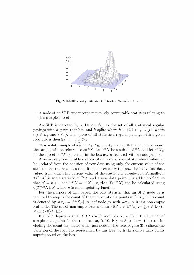
Fig. 2. R-MRP density estimate of a bivariate Gaussian mixture.

– A node of an SRP tree records recursively computable statistics relating tothis sample subset.

An SRP is denoted by s. Denote Si:j as the set of all statistical regularpavings with a given root box and k splits where k ∈ {i, i + 1, . . . , j}, wherei, j ∈ Z+ and i ≤ j. The space of all statistical regular pavings with a givenroot box is then S0:∞ := lim

i→∞S0:i

Take a data sample of size n, X1, X2, . . . , Xn and an SRP s. For conveniencethe sample will be referred to as nX. Let ⊂nX be a subset of nX and let ⊂nXρv

be the subset of nX contained in the box xρv associated with a node ρv in s.A recursively computable statistic of some data is a statistic whose value can

be updated from the addition of new data using only the current value of thestatistic and the new data (i.e., it is not necessary to know the individual datavalues from which the current value of the statistic is calculated). Formally, ifT (⊂nX) is some statistic of ⊂nX and a new data point x is added to ⊂nX sothat n′ = n + 1 and ⊂n′

X = ⊂nX ∪ x, then T (⊂n′X) can be calculated using

u(T (⊂nX), x) where u is some updating function.For the purpose of this paper, the only statistic that an SRP node ρv is

required to keep is the count of the number of data points in ⊂nXρv. This countis denoted by #xρv = |⊂nXρv|. A leaf node ρv with #xρv > 0 is a non-emptyleaf node. The set of non-empty leaves of an SRP s is L+(s) := {ρv ∈ L(s) :#xρv > 0} ⊆ L(s).

Figure 3 depicts a small SRP s with root box xρ ∈ IR2. The number ofsample data points in the root box xρ is 10. Figure 3(a) shows the tree, in-cluding the count associated with each node in the tree. Figure 3(b) shows thepartition of the root box represented by this tree, with the sample data pointssuperimposed on the box.

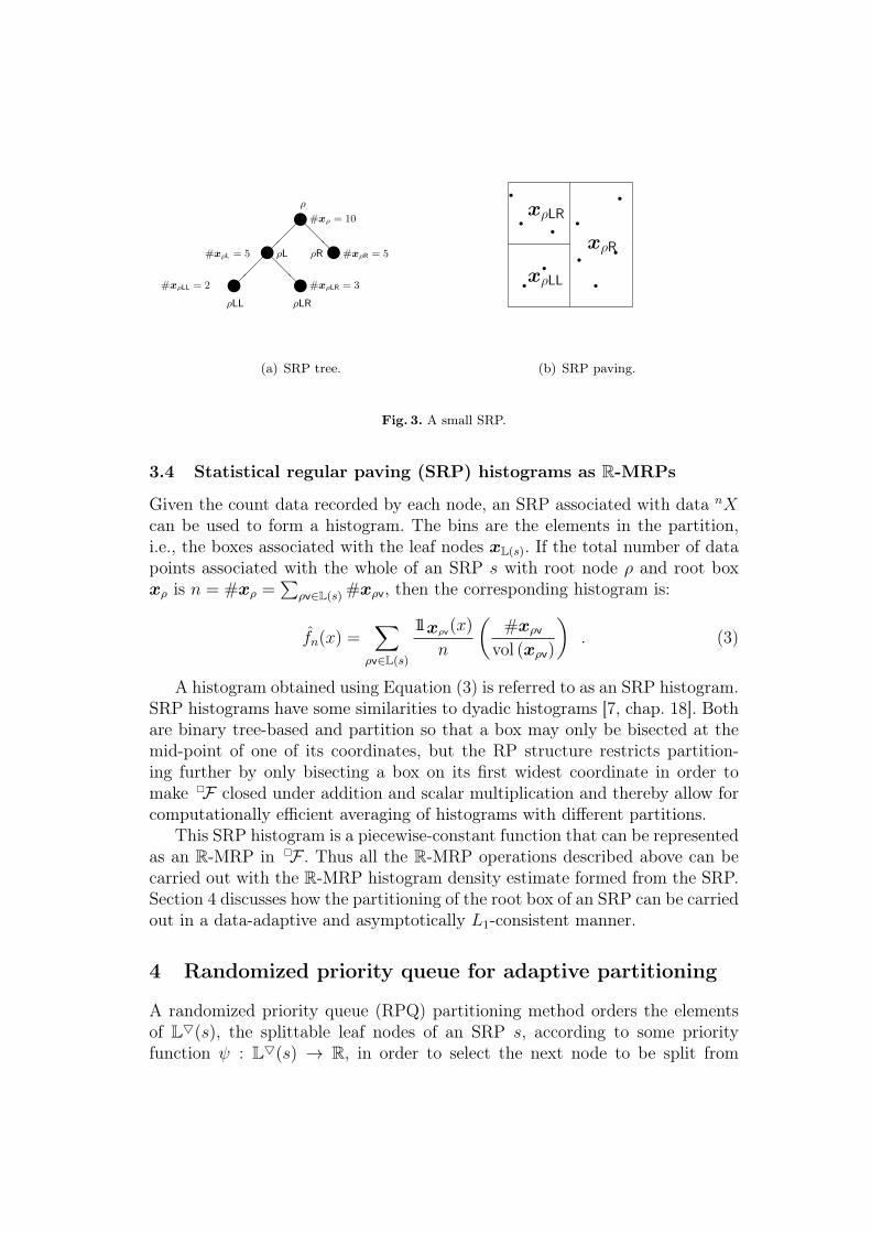
zρ #xρ = 10�

��zρL#xρL = 5

@@@zρR #xρR = 5

���z

ρLL

#xρLL = 2

@@@zρLR

#xρLR = 3

(a) SRP tree.

xρLR

xρLL

xρR

rr

rrr

rr

rrr

(b) SRP paving.

Fig. 3. A small SRP.

3.4 Statistical regular paving (SRP) histograms as R-MRPs

Given the count data recorded by each node, an SRP associated with data nXcan be used to form a histogram. The bins are the elements in the partition,i.e., the boxes associated with the leaf nodes xL(s). If the total number of datapoints associated with the whole of an SRP s with root node ρ and root boxxρ is n = #xρ =

∑ρv∈L(s) #xρv, then the corresponding histogram is:

fn(x) =∑

ρv∈L(s)

11 xρv(x)

n

(#xρv

vol (xρv)

). (3)

A histogram obtained using Equation (3) is referred to as an SRP histogram.SRP histograms have some similarities to dyadic histograms [7, chap. 18]. Bothare binary tree-based and partition so that a box may only be bisected at themid-point of one of its coordinates, but the RP structure restricts partition-ing further by only bisecting a box on its first widest coordinate in order tomake �F closed under addition and scalar multiplication and thereby allow forcomputationally efficient averaging of histograms with different partitions.

This SRP histogram is a piecewise-constant function that can be representedas an R-MRP in �F . Thus all the R-MRP operations described above can becarried out with the R-MRP histogram density estimate formed from the SRP.Section 4 discusses how the partitioning of the root box of an SRP can be carriedout in a data-adaptive and asymptotically L1-consistent manner.

4 Randomized priority queue for adaptive partitioning

A randomized priority queue (RPQ) partitioning method orders the elementsof L5(s), the splittable leaf nodes of an SRP s, according to some priorityfunction ψ : L5(s) → R, in order to select the next node to be split from

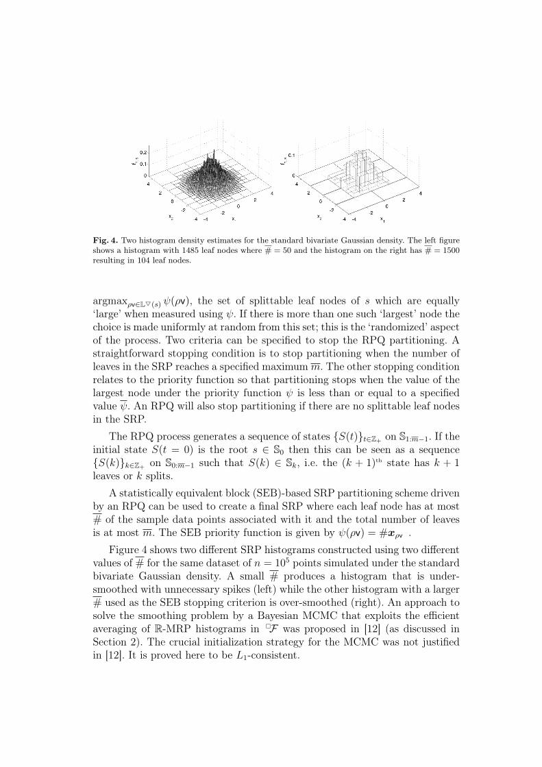
Fig. 4. Two histogram density estimates for the standard bivariate Gaussian density. The left figureshows a histogram with 1485 leaf nodes where # = 50 and the histogram on the right has # = 1500resulting in 104 leaf nodes.

argmaxρv∈L5(s) ψ(ρv), the set of splittable leaf nodes of s which are equally‘large’ when measured using ψ. If there is more than one such ‘largest’ node thechoice is made uniformly at random from this set; this is the ‘randomized’ aspectof the process. Two criteria can be specified to stop the RPQ partitioning. Astraightforward stopping condition is to stop partitioning when the number ofleaves in the SRP reaches a specified maximumm. The other stopping conditionrelates to the priority function so that partitioning stops when the value of thelargest node under the priority function ψ is less than or equal to a specifiedvalue ψ. An RPQ will also stop partitioning if there are no splittable leaf nodesin the SRP.

The RPQ process generates a sequence of states {S(t)}t∈Z+ on S1:m−1. If theinitial state S(t = 0) is the root s ∈ S0 then this can be seen as a sequence{S(k)}k∈Z+ on S0:m−1 such that S(k) ∈ Sk, i.e. the (k + 1)th state has k + 1leaves or k splits.

A statistically equivalent block (SEB)-based SRP partitioning scheme drivenby an RPQ can be used to create a final SRP where each leaf node has at most# of the sample data points associated with it and the total number of leavesis at most m. The SEB priority function is given by ψ(ρv) = #xρv .

Figure 4 shows two different SRP histograms constructed using two differentvalues of # for the same dataset of n = 105 points simulated under the standardbivariate Gaussian density. A small # produces a histogram that is under-smoothed with unnecessary spikes (left) while the other histogram with a larger# used as the SEB stopping criterion is over-smoothed (right). An approach tosolve the smoothing problem by a Bayesian MCMC that exploits the efficientaveraging of R-MRP histograms in �F was proposed in [12] (as discussed inSection 2). The crucial initialization strategy for the MCMC was not justifiedin [12]. It is proved here to be L1-consistent.

We now show that an RMRP density estimate based on an SRP created us-ing the SEB RPQ partitioning scheme is asymptotically L1-consistent providedthat # and m grow with the sample size n at appropriate rates. This is doneby proving the three conditions in Theorem 1 of [9]. We will need to show thatas the number of sample points increases linearly, the following conditions aremet:

1. the number of leaf boxes grows sub-linearly;2. the partition grows sub-exponentially in terms of a combinatorial complexity

measure;3. and the volume of the leaf boxes in the partition are shrinking.

Let {Sn(i)}Ii=0 on S0:∞ be the Markov chain formed using SEB RPQ. TheMarkov chain terminates at some state s with partition `(s). Associated withthe Markov chain is a fixed collection of partitions

Ln :={`(s) : s ∈ S0:∞, P r{S(I) = s} > 0

}and the size of the largest partition `(s) in Ln is given by

m(Ln) := sup`(s)∈Ln

|`(s)| ≤ m

such that Ln ⊆ {`(s) : s ∈ S0:m−1}.Given n fixed points {X1, . . . , Xn} ∈

(Rd)n. Let Π (Ln, {X1, . . . , Xn}) be

the number of distinct partitions of the finite set {X1, . . . , Xn} that are inducedby partitions `(s) ∈ Ln:

Π(Ln, {X1, . . . , Xn}) := |{{xρv ∩ {X1, . . . , Xn} : xρv ∈ `(s)} : `(s) ∈ Ln}| .

For any fixed set of n points, the growth function of Ln is then

Π∗(Ln, {X1, . . . , Xn}) = max{X1,...,Xn}∈(Rd)

nΠ(Ln, {X1, . . . , Xn}) .

Let A ⊆ Rd. Then the diameter of A is the maximum Euclidean distancebetween any two points of A, i.e., diam(A) := supx,y∈A

√∑di=1(xi − yi)2. Thus,

for a box x = [x1, x1]× . . .× [xd, xd], diam(x) =√∑d

i=1(xi − xi)2.We now check the three conditions for L1-consistency of the histogram esti-

mate constructed using SEB RPQ.

Theorem 1 (L1-Consistency). Let X1, X2, . . . be independent and identicalrandom vectors in Rd whose common distribution µ has a non-atomic densityf , i.e., µ � λ. Let {Sn(i)}Ii=0 on S0:∞ be the Markov chain formed using SEB

RPQ with terminal state s and histogram estimate fn,s over the collection ofpartitions Ln. As n→∞, if #→∞, #/n→ 0, m ≥ n/#, and m/n→ 0 thenthe density estimate fn,s is strongly consistent in L1, i.e.∫

|f(x)− fn,s(x)|dx→ 0 with probability 1.

Proof. We will assume that # → ∞, #/n → 0, m ≥ n/#, and m/n → 0, asn→∞, and show that the three conditions:

(a) n−1m(Ln)→ 0,(b) n−1 logΠ∗n(Ln)→ 0, and(c) µ(x : diam(x(x)) > γ)→ 0 with probability 1 for every γ > 0,

are satisfied. Then by Theorem 1 of Lugosi and Nobel (1996) our density esti-mate fn,s is strongly consistent in L1.

Condition (a) is satisfied by the assumption thatm/n→ 0 sincem(Ln) ≤ m(see Remark 1).

The largest number of distinct partitions of any n point subset of Rd that areinduced by the partitions in Ln is upper bounded by the size of the collectionof partitions Ln ⊆ S0:m−1, i.e.

Π∗n(Ln) ≤ |Ln| ≤m−1∑i=0

Ci

where i is the number of splits.The growth function is thus bounded by the total number of partitions with

0 to m− 1 splits, i.e. the (m− 1)-th partial sum of the Catalan numbers. Thepartial sum can be asymptotically approximated as ([10]):

m−1∑k=0

Ck →4m(

3(m− 1)√π(m− 1)

) as m→∞ .

Taking logs and dividing by n on both sides we get

log∆∗n(Ln)/n≤ log

(4(m(Ln)+1)

3m(Ln)√πm(Ln))

)/n

≤ 1n(m(Ln) + 1) log 4− 1

nlog 3

√(π)− 3

2nlogm(Ln).

The first and third term goes to 0 by an application of condition (a). The secondterm which is just a constant divided by n also vanishes as n→∞. Therefore,condition (b) is satisfied.

We now prove the final condition. Fix γ, ξ > 0. There exists a box x =[−M,M ]d for a large enough M , such that, µ(xc) < ξ. Consequently,

µ({x : diam(x(x)) > γ}) ≤ ξ + µ({x : diam(x(x)) > γ} ∩ x).

Using 2di hypercubes of equal volume (2M)d/2di, i =⌈log2

(2M√d/γ)⌉

with side length 2M/2i and diameter√d(2M

2i)2, we can have at most 2di boxes

in the interior of X and δ boxes at the lower dimensional boundaries of X,i.e. there are at most mγ disjoint boxes in x that have diameter greater than γ,where

mγ < 2di + δ, δ =

(2d +

d−1∑j=1

2d−j(d

j

)2ij

). (4)

By choosing i large enough we can upper bound mγ by (2M√d/γ)d + 2d +∑d−1

j=1 2d−j(d

j

)(2M√d/γ)

j, a quantity that is independent of n, such that

µ(x : diam(x(x)) > γ)≤ ξ + µ ({x : diam(x(x)) > γ} ∩ x)

≤ ξ +mγ

(maxx∈`(s)

µ(x)

)≤ ξ +mγ

(maxx∈`(s)

µn(x) + maxx∈`(s)

|µ(x)− µn(x)|)

≤ ξ +mγ

(#

n+ supx∈IRd

|µ(x)− µn(x)|).

The first term in the parenthesis converges to zero since #/n → 0 by as-sumption. For ε > 0, the second term goes to zero by applying the Vapnik-Chervonenkis theorem to boxes in IRd with shatter coefficient s(IRd, n) = 22d

[1, p. 220], i.e.

Pr

{supx∈IRd

|µn(x)− µ(x)| > ε

}≤ 8 · 22d · e−nε2/32 .

By the Borel-Cantelli lemma,

limn→∞

supx∈IRd

|µn(x)− µ(x)| = 0 w.p. 1 .

Thus for any γ, ξ > 0,

lim supn→∞

µ({x : diam(x(x)) > γ}) ≤ ξ.

Therefore, condition (c) is satisfied and this completes the proof.

Remark 1. We can choose # to be some sub-linear function of n, say nα. Thenα > 0 so that # → ∞ and α < 1 so that #/n → 0 . Now let m = nβ, thenβ > 0 so that m ≥ n/#. The above constraints imply that α + β ≥ 1. Finallyβ < 1 such that m/n→ 0.

5 Conclusions

In this paper we formalized the RP data structure and its extensions, SRP andR-MRP, and showed that by using an SEB RPQ partitioning scheme, an L1-consistent adaptive histogram can be obtained. This can be used to initializeMCMC as in [12] to obtain Bayesian smoothed density estimates.

Note that the regular paving structure places some restrictions on the den-sity estimate due to the way the bisections are selected, but has the advantageof allowing a wide range of statistical operations to be carried out efficientlyon piecewise-constant density estimate from the dense class of �F , real mappedregular pavings [5]. In addition, a collection of histogram density estimates from�F with different partitions in any dimension can be efficiently averaged evenwith large sample sizes. Up to a given prior distribution, the resulting nonpara-metric Bayesian density estimate is a smoothed R-MRP representation of theposterior sample mean with lower mean integrated absolute error than any par-ticular R-MRP histogram state visited by the MCMC algorithm [12]. A majoradvantage of the SEB-based RPQ algorithm is that, run for a limited numberof states, it can be an effective way to create an over-smoothed histogram thatreflects the major features of the density of the sample data. This gives an SRPthat provides a much better starting point for further data-adaptive partition-ing than the original, unpartitioned, SRP. By partitioning deeper into the statespace with small # we can find histograms with higher posterior densities alongthe asymptotically consistent path taken by the SEB-based RPQ Markov chain.Such high posterior states can be used to initialize the MCMC algorithm of [12]and thereby minimize the mixing time as done in [4, chap. 6].

However, a drawback of the SRP RPQ algorithm as a density estimator isthat, without some idea of the characteristics of the density to be estimated,it is extremely hard to determine suitable values for the parameters control-ling the partitioning process. As with the other greedy algorithms discussed inSection 2, the locally optimal choices made by an RPQ algorithm may be glob-ally suboptimal. An SEB-based RPQ has nevertheless been shown to be ableto produce an asymptotically consistent density estimate. Cross-validation orminimum distance estimation [2, chap. 6], or other smoothing techniques, couldpotentially be used with SRP RPQs to produce R-MRP density estimates.These possibilities are currently being explored.

Acknowledgements

This research was partly supported by RS’s external consulting revenues fromthe New Zealand Ministry of Tourism, University of Canterbury (UC) MScScholarship to JH, UC College of Engineering Sabbatical Grant and Visit-ing Scholarship at Department of Mathematics, Cornell University, Ithaca NY,USA.

References1. Luc Devroye, László Györfi, and G’aabor Lugosi. A Probabilistic Theory of Pattern Recognition.

Springer-Verlag, New York, 1996.2. Luc Devroye and G’aabor Lugosi. Combinatorial Methods in Density Estimation. Springer-

Verlag, New York, 2001.3. Alexander G Gray and Andrew W Moore. Nonparametric Density Estimation: Towards Compu-

tational Tractability. In SIAM International Conference on Data Mining, pages 203–211. SIAM,2003.

4. J. Harlow. Data-adaptive multivariate density estimation using regular pavings, with applicationsto simulation-intensive inference. Master’s thesis, University of Canterbury, 2013.

5. J. Harlow, R. Sainudiin, and W. Tucker. Mapped regular pavings. Reliable Computing, 16:252–282, 2012.

6. M. Kieffer, L. Jaulin, I. Braems, and E. Walter. Guaranteed set computation with subpavings. InW. Kraemer and J.W. Gudenberg, editors, Scientific Computing, Validated Numerics, IntervalMethods, Proceedings of SCAN 2000, pages 167–178. Kluwer Academic Publishers, New York,2001.

7. Jussi Klemelä. Smoothing of Multivariate Data: Density Estimation and Visualization. Wiley,Chichester, United Kingdom, 2009.

8. Dongryeol Lee and Alexander Gray. Fast High-Dimensional Kernel Summations Using the MonteCarlo Multipole Method. In Advances in Neural Information Processing Systems (NIPS), 21(2008), pages 929–936. MIT Press, 2009.

9. Gábor Lugosi and Andrew Nobel. Consistency of Data-Driven Histogram Methods for DensityEstimation and Classification. The Annals of Statistics, 24(2):687–706, 1996.

10. S. Mattarei. Asymptotics of partial sums of central binomial coefficients and Catalan numbers.arXiv.0906.4290v3, January 2010.

11. Jorma Rissanen, TP Speed, and Bin Yu. Density Estimation by Stochastic Complexity. IEEETransactions on Information Theory, 38(2):315–323, 1992.

12. R. Sainudiin, G. Teng, J. Harlow, and D. S. Lee. Posterior expectation of regularly paved randomhistograms. ACM Transactions on Modeling and Computer Simulation, 23(26), 2013.

13. H. Samet. The Design and Analysis of Spatial Data Structures. Addison-Wesley Longman,Boston, 1990.

14. David W. Scott. Multivariate Density Estimation. Wiley, New York, 1992.15. David W Scott and Stephan R Sain. Multidimensional Density Estimation. In C. R. Rao, E. J.

Wegman, and J. L. Solka, editors, Handbook of Statistics, volume 24, chapter 9, pages 229–262.Elsevier, Amsterdam, The Netherlands, 2005.

16. B. W. Silverman. Density Estimation for Statistics and Data Analysis. Chapman and Hall,London, 1986.

17. Charles J Stone. An Asymptotically Optimal Histogram Selection Rule. In Proceedings ofthe Berkeley Conference in Honor of Jerzy Neyman and Jack Kiefer, Vol. II, pages 513–520,Belmont, CA, 1985. Wadsworth.

18. P. Whittle. On the Smoothing of Probability Density Functions. Journal of the Royal StatisticalSociety . Series B (Methodological), 20(2):334–343, 1958.

19. Xibin Zhang, Maxwell L. King, and Rob J. Hyndman. A Bayesian Approach to BandwidthSelection for Multivariate Kernel Density Estimation. Computational Statistics & Data Analysis,50(11):3009–3031, July 2006.