Embed Size (px)
Citation preview
AMPORT $#AASO-TR-7$-"9 L V l3~ he haleng ofReetryVehicle Instrumentation
Fropared ly 7~ . LEGENDRE, W. X. OR&BOWSKY. R, G. FOWI&IR~eentry Systemns 1DIiveio~
(.he Aerispmee CorporationUT and
1. M. CASSANTOGeneral Electric Companay
31 Mlay 1978
,~ ID
Interim Report
Ulii
AI FOrCESVTEMSN COUMMAI
""I Anels Caf , . .I T
L 78 17V"~ 6
This interim report was subinitteet by ihe Aerospace Corporatien,
El SegundG, CA 90245, under Contract F04701-77-C-0078 with the Space and•Missile Systems Orgznization, Deputy for R~eentry Systems, P. O. Box 92960,
Worldway Postal Center, Los Angeles, CA 90009. It was reviewed and
approved for The Aerospace Corporation by R. E. Herold, Reentry Systems
Division. The project officer was Capt. Haroid A. Careway, SAMSO (RSSE).
This report has been rev'*.wed by the Information Office (01) and
is releacable to the National Technical Information Service (NTIS). At NTIS,
it will be available to the genera' public, including foreign nations.
This technical report has been reviewed and is approved for publica-
tion. Publication of this report does not constitute Air Force approvAl of the
report's findings or conchlaions. It is published only fur the exchange and
stimulation of ideas.
Harold A. C 7reway, Capt, JJ rres M. .c(erxiaack tProject Officer C _ hiet, Reentry Technology Division
Deputy for Reentry Systems Deputy for Reentry Systems
FOR THE COMMANDE14
I Col"Directoz, Syatems TechnoloDepoty for Peentry Svsters
UNCLASSIFIEDSECURITY ;ASIVICATION OF THIS PAGE (VU,.. Daea Enteredt)
PAG READ INSTRUCTIONSq PORT DOCUMENTATIO" G BEFORE COMPLETING FORM
M 1 2. GOVT ACCESSION NO. S. RECIPIENT'S CATALOG NUMBER1 SAMSO TR-78-99
TITLE b. TYPE OF 6EPORT & PERIOD COVERED
NHLLENGE OF_1kEENTRY)ZVEH1CLE Interim
AUIWPhillip J. Legendre., WalsR rabowsky,
qMRoy *Fowler , F1047/Xi-77-C-40W8J Jhn M. C seSanto
9. PEFRI0OGNZTO AME ANO ADDRESS 10. PROGAM EMENT. PROJECT. TASK
The Aerospace CorporationEl Segundo, Calif. 90245
11. CONTROLLING OFFICE NAME AND ADDRESS
14. MONITORING AGENCY NAME & ADDRESS(if different from, Controlling Office) IS. SECURITY CLASS. (of this report)4
Space and Missile Systems Organization UnclassifiedAir Force Systems CommandLos Angeles Air Force Station 158. DECL ASSI FICATION/ DOWN GRADING
Los Angeles, Calif. 90009 ______________ j16. DISTRIBUTION STATEMENT (of this Report)
Approved for public release; distribution unlimited.
17. DISTRIBUTION STATEMENT (of the abstract entered In Block 20, it different from Report)
NkI$. SUPPLEMENTARY NOTES
V1 It. KEY WORDS (Continue on reverse side if necessay old Identify by block numnber)
Reentry Vehicles BRAG Sensor Off-Board InstrumentationInstrumentation Roll Rate Gyro TRADEX RadarThermocouples Accelerometer ALTAIR RadarRAT Sensor Magnetometer Recession MeasurementjSeedants Off-Board Radar Shape Change Measurement
lpI AOSTRACT (Continue an revaere aide it necessary and Identify by block nusiber)
'his tutorial presents a summary of the environments, problems, and per-formance of the on-board instrumentation used on the U. S. Air Force Spaceand Missile Systems Organization (SAMSO) flighit test programs to measurereentry vehicle (RV) performance. In addition, a brief description of theoff-board instrumentation will be proesented. In RV instrumentation, the
s pecific discipline performance areas covered are the thermodynamic Endthe aerodynamic. Within the aerodynamic dis.ilpline are the group of instru-ments concerned with RV dynaimics (gyros, magnetometers, etc.) and
00FR- 4 UNCLASSIFID.~E~Ijjcltv * itToPPL"0Dt
UNCLASSIFIEDSECURITY CLASSIFICATION OF THIS PAKE(WIhu Data RE-teq.IS. KEY WORDS (Continued)
Temperature HistoryBackface TemperatureVehicle DiagnosticsAngle- of-Attack History
ASSTRACT (Continued)
with RV fluid dynamic measurements (boundary layer transition andprogression sensors, etc. ). The thermodynamic instruments include radia-tion sensors, multiwire isothermal thermocouples, optical seedants,acoustic sensors, calorimeters, etc. The overriding objective of thistutorial is to provide the instrumentation supplier with a detailedfeeling for SAMSO's RV instrumentation problems so that the supplierwill be able to propose better instruments to solve these problems.
UNCLASSIFIED
- SECURITY CLASSIFICATION OF TIMM PAIIIIIM~aM DOMe bRteuM
PREFACE
The material reported in this tutorial was developed from various
1 reentry vehicle instrumentation programs sponsored by the United States
Air Force Space and Missile Systems Organization (SAMSO) during the past
15 years.
The authors wish to thank the following individuals for their assis-
tance in preparing this presentation:
1) Dr. R. Hallse, Mr. R. Herold, and Ms. R. Pervorse of
The Aerospace Corporation.
2) Mr. C. Droms, Mr. M. DiGicamo, Mr. H. Van Dusen,and Mr. R. Kriete-" of the General Electric Company.
Special thanks to Mr. F. Yocum and N. Satin of GE for their support
of the various flight instrumentation flown to obtain the needed data.
C apecial thanks are also extended to Mr. R. Mortensen of TheAerospace Corporation and Capt. H. Careway, SAMSO/RSSE, who conducted
the detailed reviews and critical proofreading of this tutorial. In addition,!•the authors would like to thank Capt. M. Elliott, Lt. Col. R. Jackson and
Capt. T. Graham of the Air Force (SAMSO) who supported the special instru-
mentatioý.. flown and supportive analysis on the GE reentr7 vehicle.
ft. howL
I- I
................................................
F"
I .....
.......
0o,,.............
....
.... ..... ..
AYA .t-
CONTENTS
PREFACE ........................................ I
A INTRODUCTION ................ ............ 13
2. THERMODYNAMIC INSTRUMENTATION ............ 17
2. 1 General ................................. 17
2.2 Nosetip Specific ........................ 17
2.3 Backface Temperature Measurement .............. 18
2.4 In-Depth Temperature Measurement .............. 20
2.5 Breakvire Ablation Gage .... .... ........... 20
2.6 Seedants ............ .. ................ 21
2.7 Radiation Transducer Sensor ..... .............. 22
2.8 Backscatter Radiation Ablation Gage ............. 23
2.9 Light Pipe ............................. 24
2.10 Analog Resistance Ablation Detector ............. 25
2. 11 Acoustic Instrumentation ..................... 26
2. 12 Heatshield Specific ................. ...... .... 27
2. 13 Makewire and Breakwire Gages ............... 28
2. 14 Radioactive Tracer Technique .................. 28tr 2.15 In-Depth Temperature Techniques ............... 29
2.16 Measurement Planning .......... ......... 312.17 Analytical Procedures and Data Usage............. 32
3. AERODYNAMIC AND VEHICLE DYNAMICINSTRUMENTATION .................. ........... 55
3. 1 Purpose and Introduction ........................... 55
3.2 Flight Instrumentation Principles ................ 56
4. AERODYNAMIC/FLIGHT MECHANIC DATA .............. 73
4. 1 Introduction ....... ..... .0 6 ... ........ 734.2 Drag ...... . . . . . . . . . . . ...... 73
4.3 Roll Performance ............ ....... ...... 74
-3-
CONTENTS (Continued)
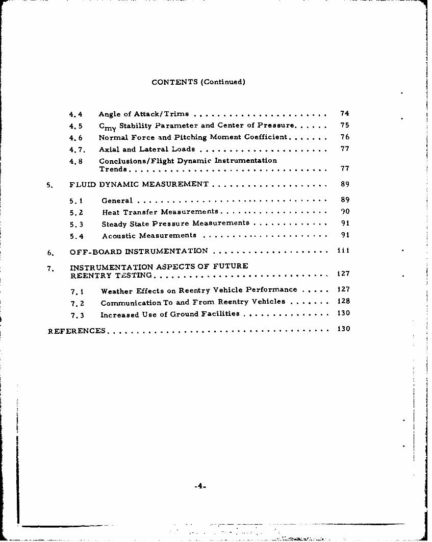
4.4 Angle of Attack/Trims ........ .. . .. .. .. .. ... 74
4. 5 CY Stability Parameter and Center of Pressure..........75
4. 6 Normal Force and Pitching Moment Coefficient. . ...... 76
4.7. Axial and Lateral Loads....................... . .. 77
4. 8 Conclusions/ Flight Dynamic Instrumentation
Trends............................. . . ... 77
5. FLUID DYNAMICGMEASUREMENT .................... 89
5.1 General.........................89
5.2 Heat Transfer Measurements..........................90
5. 3 Steady State Pressure Measurements..................91
5.4 Acoustic Measurements..............................91
6. OFF-BOARD INSTRUMENTATION ..................... tit
7. INSTRUMENTATION ASPECTS OF FUTUREREENTRY TZ STING. . ... . .. . .. .. . . ..... ....... 127
7. 1 Weather Effects on Reentry Vehicle Performance i . 17
7.2 Comnmunication To and From Reentry Vehicles......... 128
7. 3 Increased Use of Ground Facilities .......... ..... 130
REFERENCES .......................... ......... .. 130
-4-
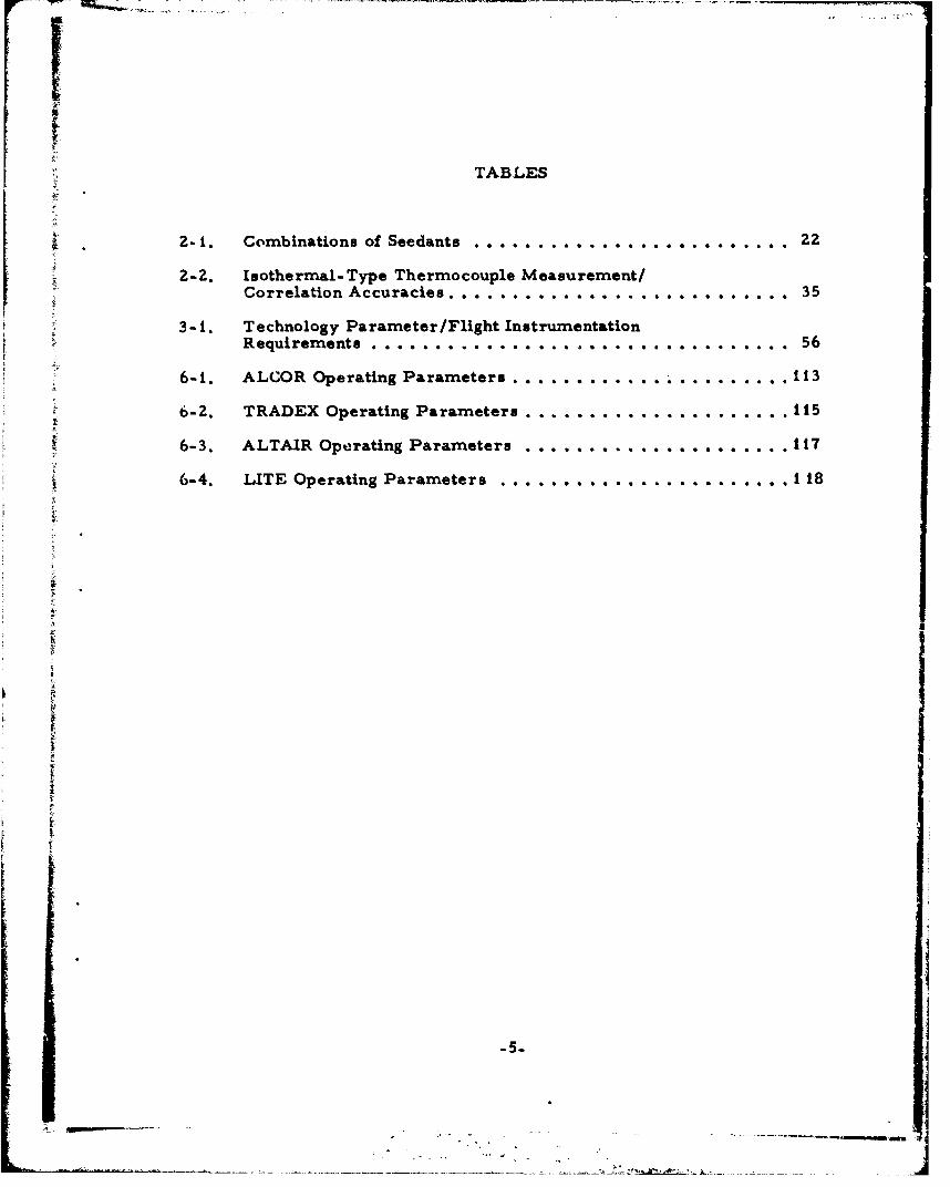
TABLES
2- 1. Combinations of Seedants ................... 22
2-2. Isothermal-Type Thermocouple Measurement/Correlation Accuracies ............ . .. ... . ... .. ... 35
3-i. Technology Parameter /Flight InstrumentationR equiremnents . ....... ......... .. ........ 56
6-it. ALCOR Operating Parameters ................ ..... *.113
6-2. TRADEX Operating Parameters .................... 115
6-3. ALTAIR Operating Parameters ....,. . . ... . . ..... 117
6-4. LITE Operating Parameters . .. .. ........... .. .. . .. 1 18
OE
t
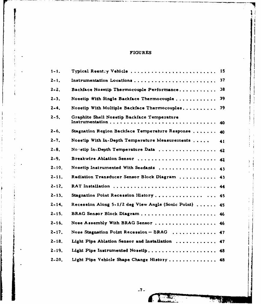
FIGURES
1-1. Typical Reent.y Vehicle ........................ 15
2- t. Instrurmentation Locations ........................ 37
2-2. Backface Nosetip Thermocouple Performance ............ 38
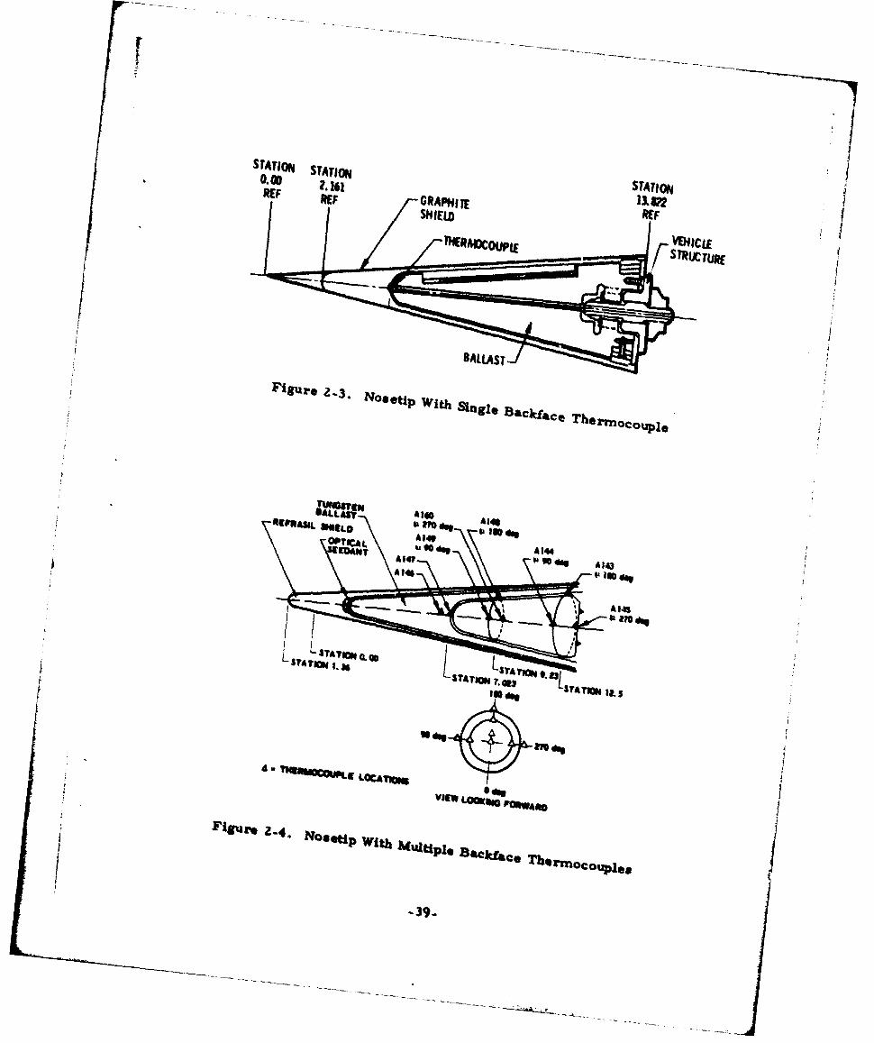
2-3. Nosetip With Single Backface Thermocouple............. 39
2-4. Nosetip With Multiple Backface Thermocouples .......... 39
2-5. Graphite Shell Nosetip Backface TemperatureInstrumentation ..................... .......... . 40
2-6. Stagnation Region Backface Temperature Response ....... 40
2-7. Nosetip With In-Depth Temperature Measurements .... 41
2-8. No.etip In-Depth Temperature Data ................. 42
2-9. Breakwire Ablation Sensor .................... 42.
2-10. Nosetip Instrumented With Seedants ..................... 43
2-11. Radiation Transducer Sensor Block Diagram . 43
2-12. RAT Installation ... .......................... 44
2-13. Stagnation Point Recession History .................. 45
Z-14. Recession Along 5-1/2 deg View Angle (Sonic Point) ....... 45
2-15, BRAG Sensor Block Diagram ...................... 46
2-16. Nose Assembly With BRAG Sensor ....... 46
2-17. Nose Stagnation Point Recession- BRAG ............ 47
2-18. Light Pipe Ablation Sensor and Installation ............ 47
2-19. Light Pipe Instrumented Nosetip .................... . 48
2-20. Light Pipe Vehicle Shape Change History ............... 48
.-7
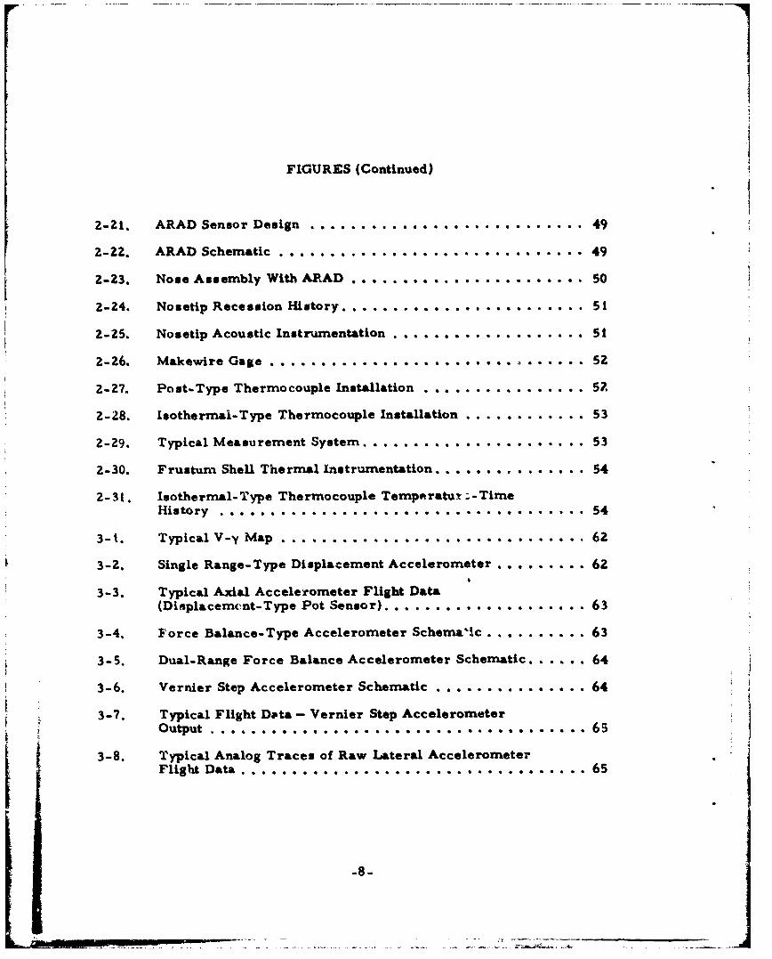
FIGURES (Continued)
2-2t. ARAD Sensor Design .............................. 49
2-22. ARAD Schematic .... . ..... . ... ...... ....... 49
2-23. Nose Assembly With ARAD ....................... 50
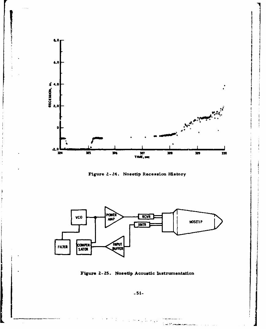
Z-24. Nosetip Recession History .... ..... ............ 51
2-25. Nosetip Acoustic Instrumentation .................. 51
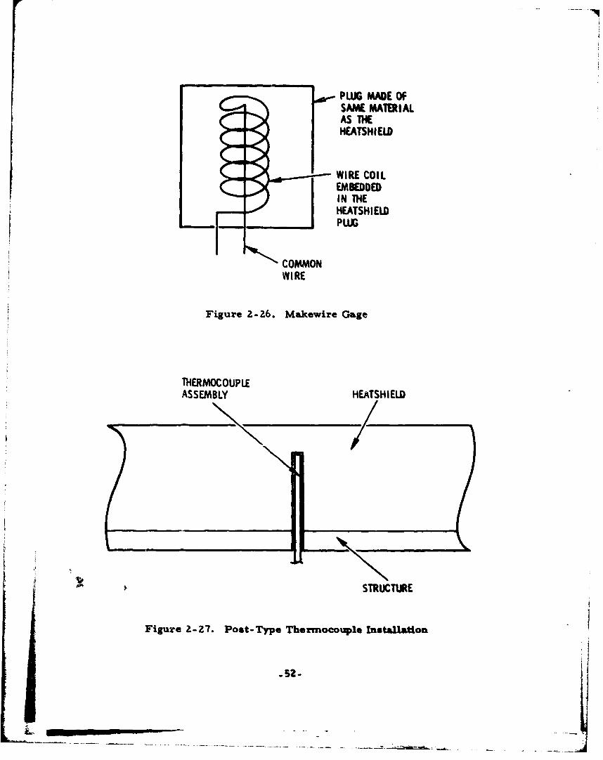
2-26. Makewire Gage ..... ...... ................... 52
2-27. Post-Type Thermocouple Installation ............... 5,
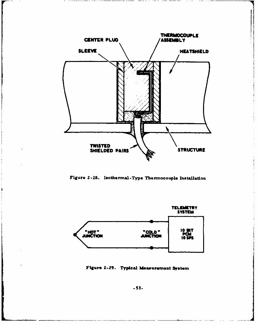
2-28. Isothermai-Type Thermocouple Installation ............ 53
2-29. Typical Measurement System ........................ 53
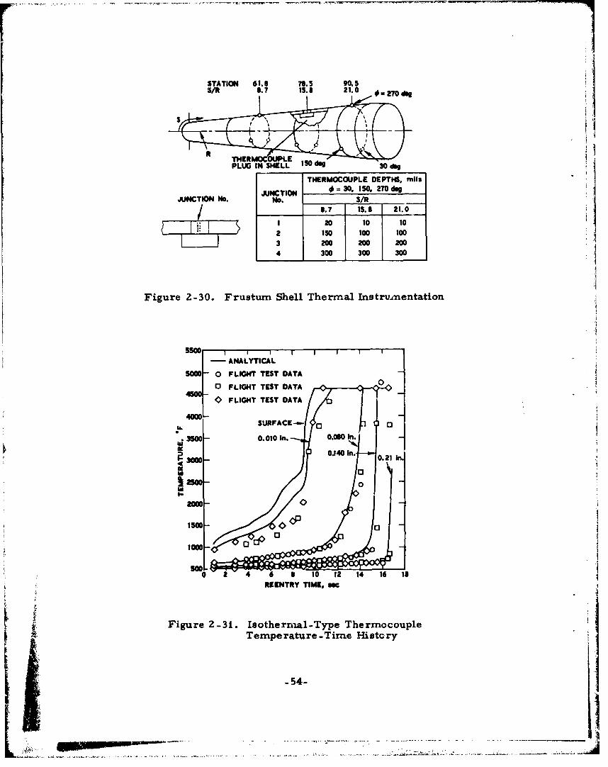
2-30. Frustum Shell Thermal Instrumentation ........ to ... 54
2-31. Isothermal-Type Thermocouple Tempe ratur;-TimeHistory . ....... ... ..... 0 .. .... ....... 54
3-t. Typical V-y Map ................ 0 ...... 62
3-2. Single Range-Type Displacement Accelerometer ......... 62
3-3. Typical Axial Accelerometer Flight Data(Displacement-Type Pot Sensor) .................... 63
3-4. Force Balance-Type Accelerometer Schema'lc ........... 63
3-5. Dual-Range Force Balance Accelerometer Schematic ...... 64
3-6. Vernier Step Accelerometer Schematic ............ 64
S3-7. Typical Flight Dota - Vernier Step Accelerometer, output ...................... ... .. ... .. 65
3-8. Typical Analog Traces of Raw Lateral AccelerometerFlight Data ............... ........... . ........ 65
g-8
!
FIGURES (Continued)
4 4
3-9. Typical Lateral Accelerometer Showing TrimBuildup ..... . .............. * ............. ...... 66
3-10. Pitch and Yaw Rate Gyro ............. ........ 66
3-I1. Dual-Axis Rate Gyro ......... 67
3-12. Raw Flight Data for Pitch and Yaw Rate Gyro From aTypical Reentry Vehicle ........................ 68
3-13. Raw Roll Rate Flight Data for a Typical Reentry Vehicle ... 68
3-14. Magnetometer .. ............................... 69
3-15. Typical Raw Magnetometer Flight Data ............... 69
3-t6. Potentiometer Pressure Sensor (Early GenerationSteady State) .......... .. .............. 70
3-17. Flight Pressure Sensor .... ..................... 70
3-18. Pressure Sensor/Port Flight Experiment ............... 71
3-19. Capacitance Pressure Sensor ....... .............. 71
3-20. Transition Indicators (Flight B) ........... ......... 72
3-21. Low Range Base Pressure Data .................. 72
4- 1. Typical Drag Component Buildup ....... 79
4-2. Flight Test Pressure Data ........................ 80
4-3. Typical Flight Test Data - Measured Drag ComponentsSvs Altitude .......... 0..........0.............
4-4. Roll Rate vs Heatshield Type and Altitude .............. 82
4-5. Early Buy Roll Torque Statistics ................... 83
4-6. Total Angle-of-Attack History ...................... 83
-9-
FIGURES (Continued)
4-7. Petal Plot for a Typical Flight Test ................. 84
4-8. C vs Altitude ...... ... ..................... 84
4-9. Vehicle Dynamic Schematic ................... 85
4-10. Nominal Angle-of-Attack History ................. 85
4-11. Normal For:e and Pitching Moment Histories ........... 86
4-1Z. Flight Test Analysis (Angle-of-Attack Reconstruction) ...... 86
4-13. Typical Axial and Lateral Load Histories ............ 87
4-14. Magnetometer Data ............................ 87
5-i. Rate (AT) Gage Installation in Heatehield .............. 96
5-2. Rate and Integration Calorimeter Gages Installationin Heatshield .................... ............ 96
5-3. Hycal Detector Principle of Operation ................ 97
5-4. Calorimeter ................................. 97
5-5. ATDetector Principle of Operation ........ 98
5-6. Internal Installation of Rate Calorimeter: ............. 98
5-7. Thermal Transition Detectors .................. 99
5-8. Summary of Transition Data ...................... 99
5-9. Transition Front Progression and Acoustic SensorResponse (Ground Test Data) ...................... 100
5-j0. Transition Sensor Locations (Flight A) ............... 100
5-1i. Piezoelectric Acoustic Gage for FluctuatingPressures (Early Generation) .......... .......... o01
5-12. Transition Noise (Flight A) .......... t10
-10-
FIGURES (Continued)
5-13. Transitton Onset From Acc,ýPtic Data (Flight A) ......... 102
5-14. Acoustic (Fluctuating Pressure) Flight Data Showing"Transitio i Onset (Flight B) ......................... 102
5-15. Acoustic Flight Data (Flight B) ....................... 103
5-16. Flight Preasure iensor .......................... 103
5-17. Present Generation (1976) Miniaturized IntegratedPressure Transducer for Steady State andFluctuating (Acoustic) Pressures ................... 104
5-18. Kulite-Ported Acoustic Gage ...................... 104
5-19. Dual-Band Pressure Measurement System forFlight Experiment ........ ............................. 105
5-20. RV Flight Tesl. Pressure Sensor Overview History ......... 106
5-21. Fluctuating Pressure Time Histories ................ 106
5-_2. Flight Test Data 6howing Simultaneous Measurementof Fluctuating and Steady State Pressure FromSame Sensor/Port ............................. 107
5-Z3. BLAM Detector Principle of Operation ............... 107
5-24. Transition Acoustic ........................... 108
5-Z5. Internal RV .................................... 108
5-26. Kaman (BLAM) Transducer Output ............. . .. 109
5-27. Kaman Detector ............. . .............. . 109
5-28. Nonported Acoustic Sensor ...................... 110
6- 1. KREMS Instrumentation ......................... 121
6-z. Kwajalein Missile Range ......................... 12
6-3. ALCOR........................................ 122
,...----.~-...
FIGURES (Continued)
6-4. ALCOR Sensitivity ............... . ............ 123
6-5. TRADEX Sensitivity ........ .............. 123
6-6. ALCOR/TRADEX Threshold Water Content Levels ....... 124
6-7. ALTAIR .................................. 1256-8. LITE Sensitivity to Ice Cloud ......... 0 .......... 1 26
6-9. High-Altitude Weather Aircraft ............... 126
7-i. Particle Measurement Radar .................. 132
A
j .t ... - - - .. -. -

1. INTRODUCTION
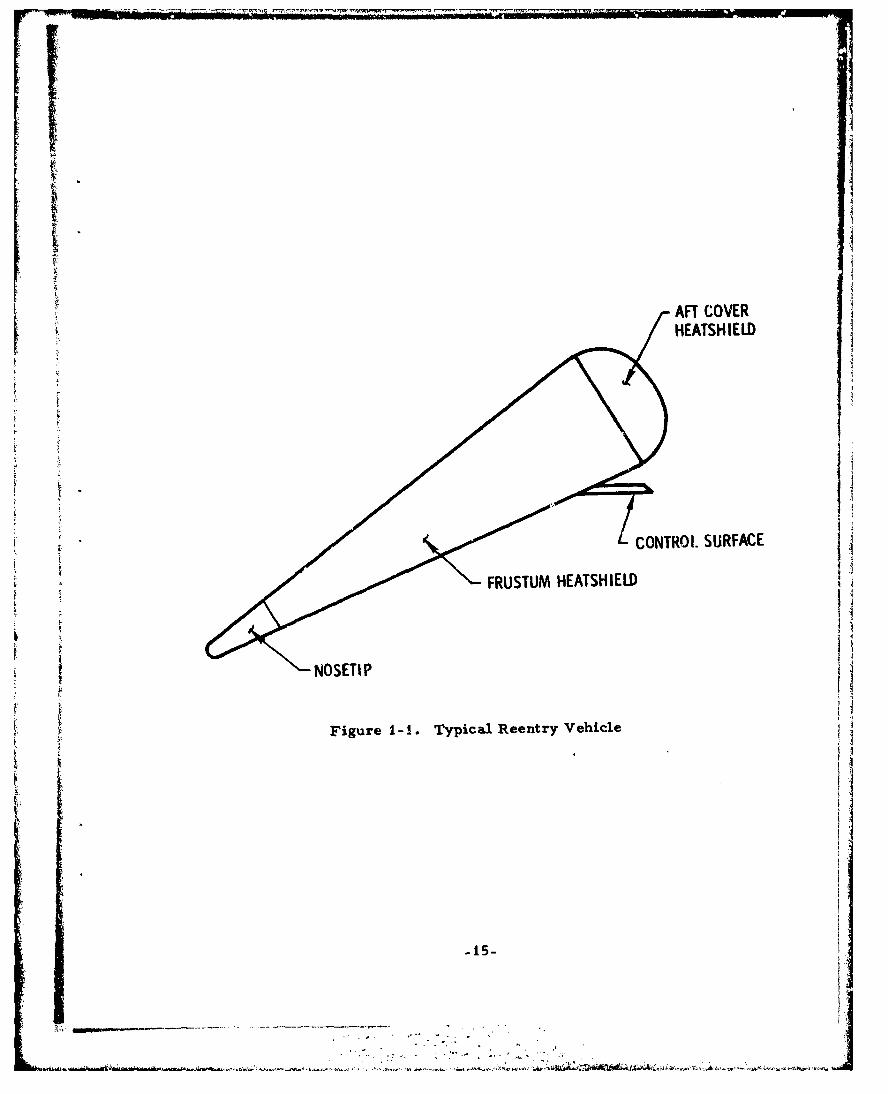
Each Space and Missile Systems Organization flight test programhas specific program objectives to be met. The flight performance evalua-tion of an experimental reentry vehicle (Figure I-1) is identified as a numberof detailed flight test objectives where it is required to obtain sufficient
flight test data for application to future operational reentry vehicles. Atypical list of detailed flight test objectives may include the following:
a. Nosetip performance as measured by recession andshape change sensors
b. Frustrum and aft cover heatshield performance asmeasured by surface recession and in-depth temperaturehistories, steady state and acoustic pressure histories,surface heat flux histories, and boundary layer onsetand progression from laminar to turbulent flow
c. Control surface shape change and surface pressuredistribution histories as measured by the same instru-ments used for the frustum and aft cover heatshields
d. Vehicle internal temperaturese. Vehicle dynamic performance as measured by on-board V
instrumentation and as observed by off-boardinstrumentation
f. Vehicle structural performance as measured by bothon-board and off-board instrumentation.
g. Vehicle observables, signature characteristics, andaccuracy as measured by off-board instrumentation
The summary of detailed flight test objectives, the measured andderived parameters required to verify the attainment of the flight test objec-tives, and the instrumentation with the associated accuracies required for thedirect measurements are outlined in a document for each flight called the9IDetailed Flight Test Plan (DFTP).
-13-
I
The typical RV reenters the earth's atmosphere at velocities
betvreen 18,000 and 25,000 fps (5490 and 7625 rn/sec). These velocities
yield th•b following representative severe environments enrountered by the
RV
a. PIs Stagnation Point Pressure, 200 atm.2b. Q , Stagnation Point Heating, 20,000 Btu/ft -,sec
(2'.29 X E + 08 W/m 2 ).
c. H., Stagnation Point Enthalpy, 8000 to 12000 Btu/lb(1.86 x E + 07 to 2.2Z X E + 07 J/km).
d. P, Heatshield Pressure, 2 to 20 atm (about 5 to10 percent of Ps).
e. Q, Heatshield Heating, 500 to 2500 Btu/ft -sec(5.76 x E + 06 to 2.84 X E + 07 W/m 2 ) (about5 to 10 percent of Qs).
sf. Surface Temperatures, 7000°R (3900°K).
g. Vibration Amplitudes to 2.0 g 2 /Hz in thrý 20 Hz to4 kHz frequency range and an overall level of90 g's rms for components attached to the nosetip.The levels experienced by components attached tothe heatshield are a fraction of those attached to thenosetip.
h. Acceleration loads up to 200 g's.
A typical reentry from 300, 000 ft (275 kin) to impact takes from
30 to 45 sec depending on the reentry angle, shape, weight, etc., of the
RV.
-14-
Iti
AFT COVERI HEATSHIELD
iiCONTRO SURFACE
S• • FRUSTUM HEATSHIELD
' i'
i •- NOSETD P
I Figure -•-1. Typical Reentry Vehicle
SAs_
2. THERMODYNAMIC INSTRUMENTATION
2.1 GENERAL
Thermodynamic instrumentation is concerned primarily with
instrumentation of the nosetip, frustum and aft cover heatshield, internal
heating, and control surfaces, if any. Generally, the types of instruments
required for the nosetip are not applicable to the heatshields or control sur-
faces. Nosetip instrumentation usually measures through large thicknesses
of material (over 30.5 cm, I ft, in a few extreme cases) whereas heatshield
and control surface thicknesses are relatively thin (1. 27 to 5.08 cm, 0.5 to
2. 0 in.). The internal heating measurements are made usually with
0 to 500°F (-17 to 226* C) thermistors and have presented no problems over
the past decade. The nosetip and heatshield areas that do present problems
will be dealt with in this tutorial.
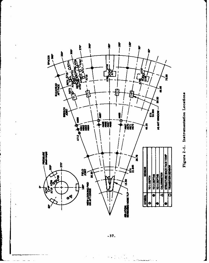
A typical RV thermodynamic instrumentation plan is presented in
Figure 2-i, and the meaning of Figure 2-1 will develop as this section of
the tutorial progresses.
2.2 NOSETIP SPECIFIC
As discussed in Reference 1, the measure of nosetip performance
has progressed through a number of stages over the past 15 years. Per-
formance was initially measured in termns of determining nosetip survival to
a specified altitude. Next, the measure of performance was the nosetip
recession history, and now nosetip performance is measured in terms of its
shape change history. In the latter case, the nocetip recession history and
survival altitude determination are byproducts of the shape change history
measurements. This refinement in nosetip performance determination has
resulted in the evolution of vastly improved nosetip instrumentation.
Many complex nosetip materials were developed, and each material
usually required a unique instrument to measure performance although some
-07-
types of nosetips made from different materials did use similar instruments.
In general, the plastic ablative nosetips, like the carbon phenolics (CP) and
the quartz phenolics (QP) can be drilled and fitted with thermocouples,
radioactive sources, etc., without seriously degrading the nosetip thermo-
dynamic performance. On the other hand, the refractory nosetip, like
graphitic nosetips, cannot normally be drilled without reducing their flight
performance due to their sensitivity to thermal strain. The newer carbon-
carbon nosetips fall in between.
Nosetp instrumentation state of the art to 1975 was reviewed in
Reference 1, and some of those systems discussed then and in this tutorial
ale covered individually in more detail in References 2 through 12 inclusive.
Also, the instrumentation installation problems associated with some of the
more recently developed nosetip materials are presented in References 9,
13, 14, and 15.
2..3 BACKFACE TEMPERATURE MEASUREMENT
Reentry vehicle project engineers have traditionally been concerned
with the possible degradation of nosetip performance on their reentry vehicles
because of discontinuities in the nosetip material due to instrumentation
insltallation. During the mid-1960s, the only nosetip instrumentation on some
of the SAMSO Programs was one or more thermistors, resistance thermo-
meters, or thermocouples mounted on the ballast to which the nosetip was
attached. The purpose of these instruments was to measure any temperature
rise in the event of nosetip failure. Usually, if the nosetip performed as pre-
dicted, these thermistors, resistance thermometers, or thermocouples would
show little or no temperature rise. If, on the other hand, the nosetip was not
performing as predicted, but was still functioning, the ballast-mounted instru-
ments would usually indicate a temperature history that exceeded the predicted
range and that either rose to less than the maximum range of the instrument
(usually 00 to 5000 F) (-17 to 226 C) or reached the maximum range of the
instrument at a moderate rate of change of temperature time. In the case of
-18-
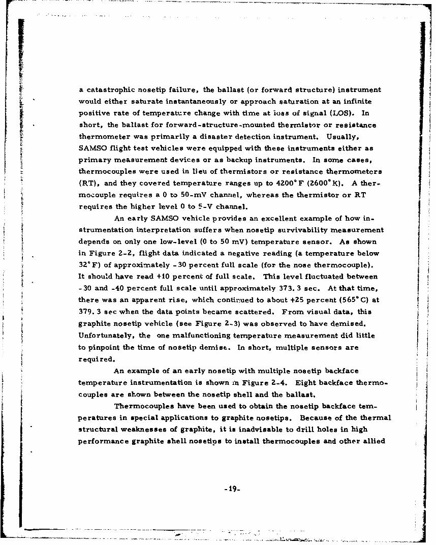
a catastrophic nosetip failure, the ballast (or forward structure) instrument
would either saturate instantaneously or approach saturation at an infinite
positive rate of temperature change with time at ioss of signal (LOS). In
short, the ballast for forward-structure-mounted thermistor or resistance
thermometer was primarily a disaster detection instrument. Usually,
, SAMSO flight test vehicles were equipped with these instruments either as
primary measurement devices or as backup instruments. In some cases,
thermocouples were used in lieu of thermistors or resistance thermometers
(RT), and they covered temperature ranges up to 4200° F (26000 K). A ther-
mocouple requires a 0 to 50-mV channel, whereas the thermistor or RT
requires the higher level 0 to 5-V channel.
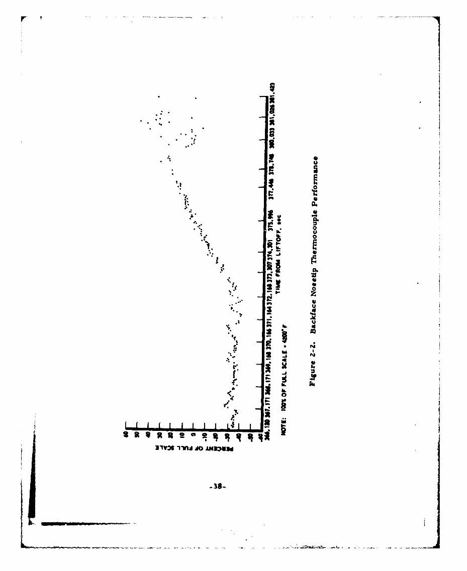
An early SAMSO vehicle provides an excellent example of how in-
strumentation interpretation suffers when nosetip survivability measurement
depends on only one low-level (0 to 50 mV) temperature sensor. As shown
in Figure 2-2, flight data indicated a negative reading (a temperature below
320 F) of approximately -30 percent full scale (for the nose thermocouple).
It should have read +10 percent of full scale. This level fluctuated between
-30 and -40 percent full scale until approximately 373.3 sec. At that time,
there was an apparent rise, which contirued to about +25 percent (5650 C) at
379. 3 sec when the data points became scattered. From visual data, this
graphite nosetip vehicle (see Figure 2-3) was observed to have demised.
Unfortunately, the one malfunctioning temperature measurement did little
to pinpoint the time of nosetip demise. In short, multiple sensors are
required.
An example of an early nosetip with multiple nosetip backface
temperature instrumentation is shown vn Figure 2-4. Eight backface thermo-
couples are shown between the nosetip shell and the ballast.
Thermocouples have been used to obtain the nosetip backface tem-
peratures in special applications to graphite nosetips. Because of the thermal
structural weaknesses of graphite, it is inadvisable to drill holes in high
performance graphite shell nosetins to install thermocouples and other allied
-19-
instrumentation. Therefore, to get some measure of the graphite shell
nosetip performance, thermocouples were pressed against the interior wall
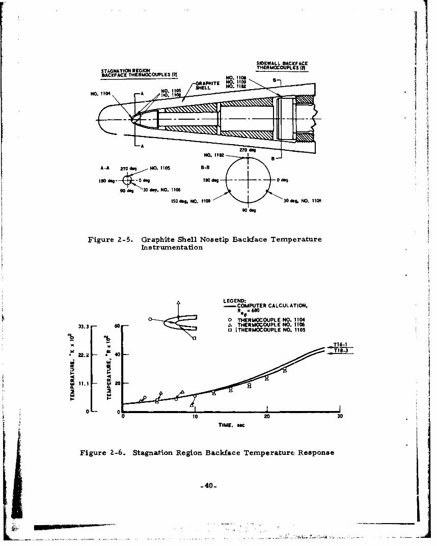
of the graphite s'-ell. On a past SAMSO Program, the backface thermocouples
were spring-loaded against the nosetip shell backface (see Figure 2-5). Theflight test temperature data for this nosetip are superimposed on the analytical
data in Figure 2-6. In this situation, the assumption was made that, if theflight test backface temperature data matched the predicted data, then the
predicted nosetip recession and shape change histories were also grossly
correct. As shown in Figure 2-6. the nosetip flight and predicted temperature
data agreed quite well.
2.4 IN-DEPTH TEMPERATURE MEASUREMENT
Some measure of nosetip thermodynamic performance was obtained
by locating thermocouples in the nosetip material. These were bayonet type
(also called post thermocouples) mounted in holes drilled parallel to the
nosetip centerline from the rear of the nosetip.
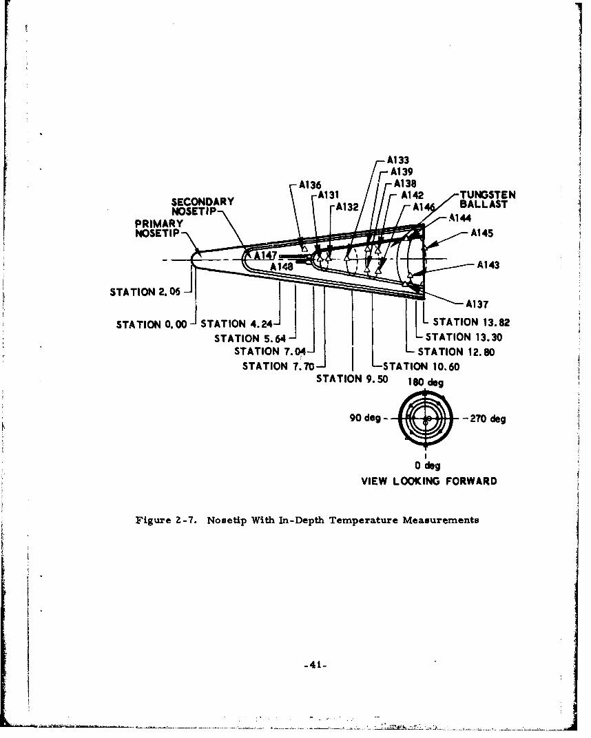
Figure 2-7 depicts a nobetip equipped with an array of 12 backface
thermocouples similar to those shown in Figure 2-4. However, in the
"Figure 2-7 nosetip, two in-depth, bayonet-type thermocouples (A147 and
A148) are located at two depths in the secondary nosetip material. In this
specific case, no temperature rise was predicted by any of the 14 sensors
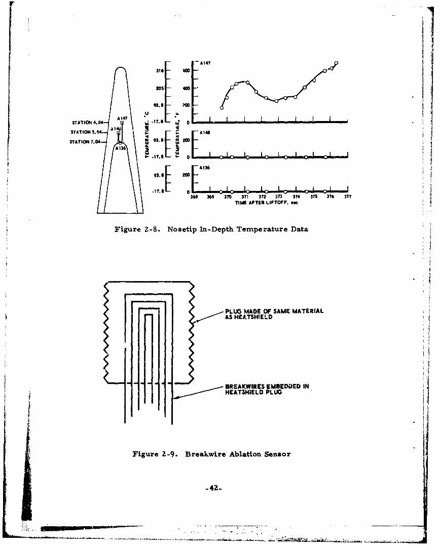
and none was indicated by the flight test data. As shown in Figure 2-8 (a
nosetip similar to that shown in Figure 2-7), one of the thermocouples did
rise significantly. This permitted the nosetip designer to compare the
measured and predicted results and redesign accordingly.
2.5 BREAKWIRE ABLATION GAGE
As discussed in Reference 16, the breakwire ablation gage isusually associated with the frustum heatshield (Figure 2-9). It has not been
very successful in this application. Theoretically, as the heatshield surface
receded and/or charred, the increasing heat entering the heatshield was
supposed to progressively melt the breakwires and break the electrical
-20-
circuit. However, on some Refrasil heatshields, the receding char layer
made excellent electrical contact between the melted wirea and gave the
erroneous readings that the surface had not yet ch.rred to a given depth.
This same principle was applied to a nosetip similar to that depicted in
Figure 2-7 except that breakwires, in lieu of in-depth, bayonet-type th~rmo-
couples, were installed #- detect secondary nosetip recession. However,
none of the breakwire thermocouples responded. This normally woul6 indicate
that the nosetip had not receded to the position of the first breakwire, but
this was not consistent with similar flights.
Both breakwire and makewire ablation gages were ground tested in
nosetips on the Carbon-Carbon Nosetip Development Program (CCND). (ii)
The ground tests indicated that both concepts functioned satisfactorily with
respect to measuring nosetip recession, but, unfortunately, the size of the
sensors degraded the carbon-carbon nosetip recession performance too much
to consider them for flight applications.
2.6 SEEDANTS
Many of the previously discussed nosetips, which were instrumented
with or..4 or more forms of thermocouples, were also instrumented with opti-
cal seedants. A seedant for RVs is a material that would be highly observable
by opt-cal ground instrumentation when vaporized by the severe thermal
environment to vhich it was subjected. Some of the seedants used are tabulated
in Table 2- t. A typical seeuant instrumentation sche'ne is shown in
FVgure 2-10. N, trace of the indium sulfiue or ytterbiur. carbonate was noted
during flight. None of the seedants was observed on a saecond vehicle that
demised due to nusetip failure, but the cesium in the cesium iodide crystal of
a sc ntillator package was observed. Similar lack of success was observed
irt other fliglits or. the same SP,,4SO program. Therefore, it was concluded
that seedants d•. iot really work and consequently were not included in the
instrumentation of succeeding RV programs.
t .I
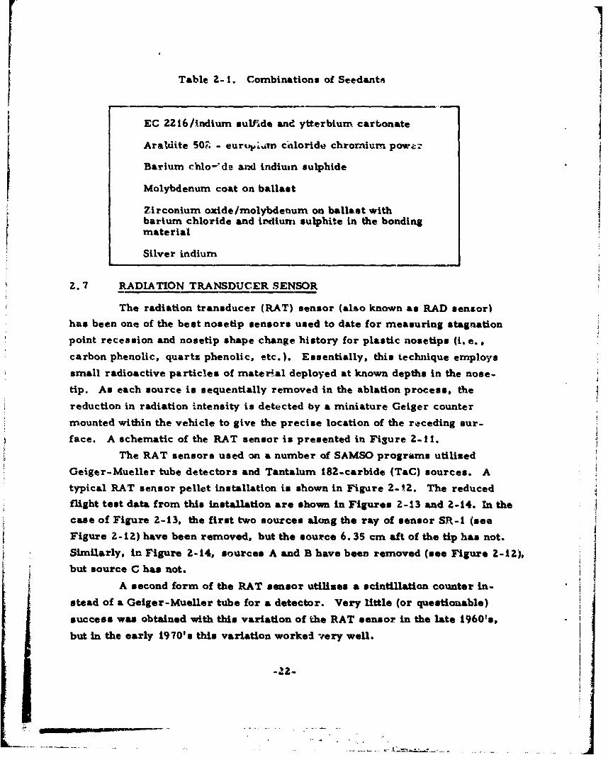
Table 2- 1. Combinations of Seedants
EC 2216/indium sulf-Ide and ytterbium carbonate
Araldite 50Z - euruplm chloride chromium powz
Barium chlo--de and indium sulphide
Molybdenum coat on ballast
Zirconium oxide/molybdenum on ballast withbarium chloride and indium sulphite in the bondingmaterial
Silver indium
2.7 RADIATION TRANSDUCER SENSOR
The radiation transducer (RAT) sensor (also known as RAD sensor)
has been one of the best nosetip sensors used to date for measuring stagnation
point recession and nosetip shape change history for plastic nosetips (i. e.
carbon phenolic, quartz phenolic, etc.). Essentially, this technique employs
small radioactive particles of material deployed at known depths in the nose-
tip. As each source is sequentially removed in the ablation process, the
reduction in radiation intensity is detected by a miniature Geiger counter
mounted within the vehicle to give the precise location of the receding our-
face. A schematic of the RAT sensor is presented in Figure 2- I.
The RAT sensors used on a number of SAMSO programs utilized
Geiger-Mueller tube detectors and Tantalum 182-carbide (TaC) sources. A
typical RAT sensor pellet installation is shown in Figure 2-_12. The reduced
flight test data from this installation are shown in Figures 2-13 and 2-14. In the
case of Figure 2-13, the first two sources along the ray of sensor SR-i (see
Figure 2-12) have been removed, but the source 6.35 cm aft of the tip has not.
Similarly, in Figure 2-14, sources A and B have been removed (see Figure 2-12),
but source C has not. .1A second form of the RAT sensor utilizes a scintillation counter in-
stead of a Geiger-Mueller tube for a detector. Very little (or questionable)
success was obtained with this variation of the RAT sensor in the late 1960s,
but In the early 1970's this variation worked very well.
S-22I
In the mid- 1970's, counters based on a cadmium tellurlde (CdTe)
crystal wee developed by several RV contractors.( 1 8 , 19) These CdTe
detectors were more efficient than previous detectors thus permitting lower
nosetip radiation levels per line permitting lower nosetip radiation lejels
per line source for a given accuracy. Also, these detectors were smaller
than the Geiger-Mueller tubes, for example, and this permitted a larger
number of line sources to be installed per nosetip.
References 3, 7, 8, 9, 10 and 11 cover almost every type and phase
of RAT sensor development in detail.
A variation of the RAT sensor, called the shape change ablation
transducer (SCAT), was flown, in the early 1970's, but it was not very success-
ful. (1) Whereas the RAT sensor radiation sources were embedded wires in
the plastic of nosetips, the SCAT sensor utilized tantalum 182 diffused in a
graphite nosetip during the manufacturing process. Essentially, the SCAT
sensor consisted of the irradiated graphite nosecap, three scintillator-
photomultiplier tube gamma-ray detectors, and an electronics package to
convert the measured gamma radiation to an electrical signal. Unfortunately,
the diffused tantalum 18Z source swamped out the signal because of (a) inade-
quate sidewall shielding of the detectors or (b) redeposition of the tantalum 182
on the heatshield adjacent to the detectors.
In recent years, continuous line sources 3 ' (3.9") have been developed
to replace the pellet sources to overcome performance anomalies. (13-15) These
anomalies were caused by aggravated recession at the sites of the pellet sources
due to the presence of the sources. The amount and severity of the aggravated
recession was a function of source size, installation expedient, tolerances, ad-
hesive and the post installation cure of the adhesive. A line source integrated
into the structure of the nosetip eliminated all of the above problems.
z. 8 BACKSCATTER RADIA £ION ABLATION GAGE
The backscatter radiation ablation gage (BRAG) sensor was initially
proposed by the Gianni Controls Corporation under a General Electric Company
(GE) development contract in the early 1960's. (16, 20, ZI) In recent years,
this instrument was developed by GE and flown on many SAMSO vehicles.
-23-
........................................................
The BRAG sensor consists of a source of gamma radiation, a shield for
preventing direct transmission to the gamma-ray detector unit, the detector
unit itself, and the signal condicioning electronics (gee Figure Z-15).
A portion of the gamma radiation from the source is backscattered
from the ablation material, and a fraction of these backscattered rays reaches
the detector unit. This fraction is directly proportional to the thickness of the
ablation material at the specific time during which the measurement is
performed. The detector unit digital sensor converts the gamma rays into
electrical pulnes that are simply scaled for the telemetry (TM) bandwidth
and transmitted directly over the TM link. Figure 2-16 shows the installation
of the source, collimation hole, and detector in a nosetip. The nose stagna-
tion point recession is shown in Figure 2-17.
The primary advantage of the BRAG sensor is that it does not
require the placement of discontinuities (drilled holts, pellets, etc. ) in the
nosetip material as does the RAT sensor concept, for example. This makes
the BRAG sensor an excellent instrument for graphitic nosetips that do not
tolerate large discontinuities.
A more cetailed account of the GE BRAG sensor and its application
may be obtained from Reference 22.
Sometimes it is desirable to measure the recession of the ballast
material (usually tungsten) under the primary nosetip when this material is
exposed prior to impact. The gamma-ray source of the previously discussed
BRAG sensor will not work due to the gamma-ray attenuation qualities of
tungsten. A BRAG sensor based on a neutron source was developed, but never
flown, to cope with this application. (14)
2.9 LIGHT PIPE
NASA Langley Field developed an ablation gage in the early 1960's(16)in which the surface recession was measured by the change of light intensity.
The NASA Langley instrument is placed in a blind hole. When the hole is
uncovered during the ablative process, the light from the incandescent
ablative surface is transferred via a sapphire light pipe to a photodiode. The
electrical current produced by the photodiode is transmitted via telemetry
to the ground.
-24-
The light pipe was developed further by the Avco Corporation in the
early 1970'. for application to three-dimensional quartz phenolic (3-DQP)
nosetips. It was believed that a high number of light pipe sensors installed in
a nosetip would give sufficient data to enable the pontflight analyst to
reconstruct the novetip shape change history of the flight test n3setip.
The Avco light pipe utilizes quartz fibers to transmit the light to
the photodiode. An Avco light pipe assembly for use in a ground test is
albown in Figure Z_-18. In this assembly, bundles of seven 0. 008-In. diameter
(0. 0203 cm) quartz fibers are used to transmit the light. The surfaces of
the fibers are covered with chromium. The overall width of the assembly is
0. 040 in. (0. 103 cm); the seven light pipe assembly was developed for use
on SAMSO RVs. A typical three light pipe installation in a ground test nose-
tip is also shown in Figure 2-18.
The light pipe sensor was flown on a SAMSO vehicle in early 1973.
The 3-DQP nosetip was instrumented with 13 light pipe sensor bundles with
7 steps per bundle. The light pipe sensor installation is outlined in Fig-
ure 2- 19. Also note the other types of complementary instrumentation pre-
viously discussed in this paper. The flight test was very successful with
respect to the light pipe sensor performance where data from all 91 (7 X 13)
data points were obtained.
The reduced nosetip shape change history is presented in Figure 2-20
for the 0 deg meridian plan. Note that the 91 data points permit a more
definitive nosetip shape change history than the 25 RAT data points for the
vehicle presented in Figure 2-12.
2. 10 ANALOG RESISTANCE ABLATION DETECTOR
The analog resistance ablation detector (ARAD) was developed by
GE to determine the shape change history of ablative nosetips by determining
the nosetip recession via an analog voltage proportional to the recession.
The ARAD sensor element (shown in Figure 2-21) is a three-terminaldevice consisting of a helix of platinum tungsten resistance wire wound over
a quartz fiber-covered central platinum/conductive epoxy electrode. Quartz
fiber is also used to insulate the helix from the outer conductive shell that
is composed of platinum wires and conductive epoxy. The entire sensor Is
only 0.05 in. (0. 102 cm) in diameter and can be wound to any desired length.
-25-
The nominal impedance of the helical portion of the sensor is 7000 0 /in.
(2760 f/cm). As the surface of the nose recedes during ablation, the resis-
tive element is burned off with the resultant change in resistance giving a
continuous measurement of the heatshield thickness. For preablation testing,
the end of the sensor is coated with conductive epoxy that shorts the inner
and outer conductors to the end of the helix.
During ablation, the hot quartz serves as a movable short, complet-
ing the sensor circuit. A schematic of this circuit is shown in Figure 2-22.
A nosetip and ARAD installation are presented in Figure 2-Z3.
There were 13 ARAD sensor installations in this nosetip.
An example of ARAD data is shown in Figure 2--24 in the form of a
nos etip surface recession history.
2-1i ACOUSTIC INSTRUMENTATION
Although radiation-type sensors have been performing admirably on
SAMSO vehicles for over 15 years, there is a trend to use nonradiation sen-
sors whenever possible because of the radiation handling problems. In the
case of nosetip instrumentation, acoustic measurement devices have been
developed and are being improved to obtain nosetip recession and shape
change. (2, 5 ,6)
In these applications, a transmitter at the backface of the nosetip
sends a pulse through the nosetip, the pulse is reflected from the nosetip
surface, and the reflected wave is picked up by a receiver mounted on the
nosetip backface (Figure 2-25). The differences and lags between the trans-
mitted and received wave forms will vary as the nosetip recedes, and it is
these differences that enable the analyst to determine the resulting nosetip
recession.
In addition to measuring nosetip recession, recent flight test results
indicate that this sersor may sense boundary layer transition on the nosetip
and encounters with weather phenomena.
-26-
"it,.
<I
%I2. 12 HEATSHIELD SPECIFIC
The performance evaluation of fthe heatshield is identified as a
detailed flight test objective where it is required to obtain sufficient flight
test data for the design of future operational heatshields with a small margin
of safety (MS). Performance is usually defined as the heatshield's time
histories (surface recession and temperature). A small MS means lighter
heatshields and greater operational range. Heatshields Lhat ablate pre-
dictably and consistently indicate that the vehicle dynamic parameters (like
the center of gravity offset and vehicle moment changes due to ablation-
caused mass distribution changes), which are dependent upon the heatshield
recession, shape change, surface roughness, etc., will be predictable and
consistent. Unpredictable and inconsistent vehicle dynamics mean unpre-
dictable, inconsistent, and usually unacceptable vehicle targeting accuracies.
Control surface shape change data, which may influence body and
control surface aerodynamic designs, are valuable to the design of maneuver-
ing vehicles and their control requirements. In-flight determination of
heatshield performance. on reentry vehicles has long preiented a difficult
measurement proklem. The difficulties encountered in the measurements are
a result of the previously discussed environment, which includes high heat
flux, oxidation, and aerodynamic shear conditions. Included with these dif-
ficulties are the electrostatic and electrodynamic problems associated with
the plasma, as well as the telemetry system RF power reflected from the
plasma at the time of highest measurement interest. The response of the
heatshield to the reentry environment can include surface recession, crack- 4ing, swelling, outgassing, and other physical and chemical processes that
present severe heatshield instrument installation design problems.
Heatshield instrumentation state of the art to 1973 was reviewed in
Reference 23. Some of the heatshield instruments developed since will be
discussed briefly in this tutorial and in detail in References 24 to 26,
inclusive.
_27-
2. 13 MAKEWIRE AND BREAKWIRE GAGES
As discussed earlier in this tutorial and in Reference 16, many
measurement techniques have been considered for measuring the surface
recession of a reentry vehicle heatshield. For example, makewire (Fig-
ure 2-26) and breakwire gages (Figure 2-9) were considered in the early
1960's. In the case of the makewire gage, a continuous coil of wire was
embedded in the heatshield material and a common wire was located in the
center of the heatshield material within the confines of the coil. As the
ablated char layer increased in thickness, electrical continuity was pro-
gressively established between the wire coils and the common wire because
of the conductivity of the carbon content of the char layer. Unfortunately,
all that had been directly measured was the progression of the charing pro-
cess to the point that a current could be conducted between the coil and com-
mon ground. It was not a direct indication of surface recession.
In the case of the breakwire ablation gage, wires were installed in
a plug of heatshield material, and a current normally flowed through the
wires. As the surface receded and was charred, the increase of heat flowing
into the heatshield progressively melted the wires and broke the electrical
circuit to indicate heratshield degradation to a specific depth. Unfortunately,
the char layer in some instances made an electrical contact between the
melted wires and gave erroneous readings of char layer formation or sur-
face recession.
2. 14 RADIOACTIVE TRACER TECHNIQUE
This technique employs several small radioactive particles of
material deployed at known depths in the heatshield material in a manner
similar to that for nosetips (Figure 2-11). As each source is sequentially
removed in the ablation process, the reduction in radiation intensity is
detected by a sensing element, such as a miniature Geiger counter mounted
within the vehicle, to give the precise location of the receding surfact.
"" I
-28-
ENDWk. .
Difficulties in data interpretation are encountered using this
concept due to the statistical nature of the radiation impingement on the
Geiger counter. The "steps" produced by the removal of discrete sources
overcome, to a large extent, the statistics problem if the flight is on schedule.
Delays in flight dates cause increased system errors due to decay of the
radioactive material, with attendant degradation of the counting statistics.
Of course, some of these difficulties may be minimized by increasing the
source strength and the sampling rate.
2.15 IN-DEPTH TEMPERATURE TECHNIQUES
Thermocouples mounted at predetermined depths below the heatshield
surface provide temperature histories at the respective locations, from which
the position of the ablating surface may be deduced. The accuracy of this
system is enhanced in a high heating rate environment, where the rate of
temperature change near the surface is very high. The thermocouples
normally used are the tungsten-rhenium type, 3 to 5 mils in diameter, which
have good calibration to 4200°F (26000K) and may produce acceptable readings
as high as 50000F t3050*K). The chromel-alumel wire is sometimes used
for applications to ZZ00°F (1480'K). The use of this sensor as a recession
gage does not depend to a great extent on the accuracy of the temperaturemeasurement; however, it depends on the accuracy of the extrapolation of a
temperature-time plot to the temperature at which it is estimated that the
heatshield materiel has reached its demise. At a high rate of temperature
change, the slope is almost vertical and the time resolution of the sensor is
inconsequentially small.
Measurements of heatshield material temperature have been made
with two basic thermocouple configurations: the isothermal installation and
the bayonet- or post-type installation.
The post or bayonet configuration can be simply installed as shown
S"in Figure 2-27. Holes are drilled in the vehicle heatshield material fromr
the inside and the thermocouple is h')nded in place. The drilling of a specific
depth below the surface of the heatshield is difficult, and depth locations with
-29-
uncertainties of as much as 0.020 to 0.030 in. are normal because of the
awkward drill handling and dimensional measurement requirements involved
in drilling the holes from the inside.
An isothermal configuration is shown in Figure 2-28. The purpose
of this design is to eliminate or minimize the error inherent in the post type
caused by heat conduction down the lead wires from the hot junction. The
magnitude of this error is a function of the differences in conductivity between
the heatshield material and the thermocouple material and can be as high as
50 percent. Several isothermal plugs have been developed without the
outer sleeve depicted in Figure 2-28, and these were also flight-tested
successfully on SAMSO vehicles,
After a plug has been fabricated, the plug is X-rayed to determine
the location of the junctions below the surface of the plug. 'Using this method,
the location errors can be held to less than 0.001 in. (0.00254 cm) for the
cold heatshield.
In-flight measurement accuracy involves the accuracies of the
series elements in the data acquisition system. For the typical measurement
system shown in Figure 2-29 involving an isothermal-type thermocouple, the
uncertainties are as follows:
Hot junction < i percert
Reference junction < 0. 005 percent
TLM system < 0. 2 percent
Root sum square (RSS) of above errors =<1.1I percent
Uncertainties due to thermocouple lead wire conductivity, thermalmass, junction, lead wire shielding, insulation defy.radation, and contact ,
of the thermocouple hot junction with the heatshield material can only be
assessed by ground tests using the particular heatshield at a heating rate
that closely approximates the rate expected for the particular trajectory.
-30-
•:'• ~ ~ ~ ~ ~ ~ ~ ~ ~ ~ ~ ~ ~ ----- -[ •: ..- - - • ....... .... . . " ",... .
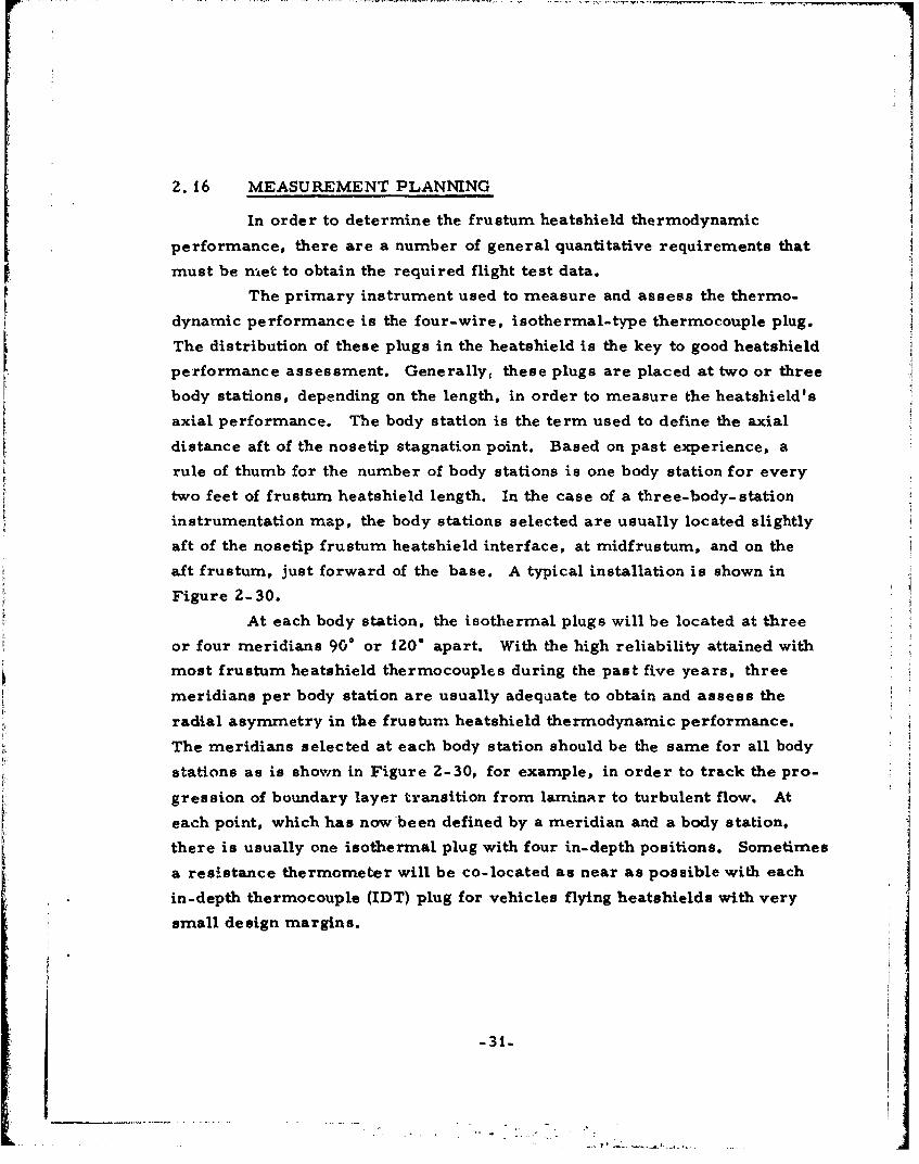
2. 16 MEASUREMENT PLANNING
In order to determine the frustum heatshield thermodynamic
performance, there are a number of general quantitative requirements that
must be rnret to obtain the required flight test data.
The primary instrument used to measure and assess the thermo-
dynamic performance is the four-wire, isothermal-type thermocouple plug.
The distribution of these plugs in the heatshield is the key to good heatshield
performance assessment. Generally, these plugs are placed at two or three
body stations, depending on the length, in order to measure the heatshield's
axial performance. The body station is the term used to define the axial
distance aft of the nosetip stagnation point. Based on past experience, a
rule of thumb for the number of body stations is one body station for every
two feet of frustum heatshield length. In the case of a three-body-station
instrumentation map, the body stations selected are usually located slightly
aft of the nosetip frustum heatshield interface, at midfrustum, and on the
aft frustum, just forward of the base. A typical installation is shown in
Figure 2- 30.
At each body station, the isothermal plugs will be located at three
or four meridians 900 or 1206 apart. With the high reliability attained with
most frustum heatshield thermocouples during the past five years, three
meridians per body station are usually adequate to obtain and assess the
radial asymmetry in the frustum heatshield thermodynamic performance.
The meridians selected at each body station should be the same for all body
stations as is shown in Figure 2-30, for example, in order to track the pro-
gression of boundary layer transition from laminar to turbulent flow. At
each point, which has now been defined by a meridian and a body station,
there is usually one isothermal plug with four in-depth positions. Sometimes
a resistance thermometer will be co-located as near as possible with each
in-depth thermocouple (IDT) plug for vehicles flying heatshields with very
small design margins.
-31-
On those programs where radiation detector (RAD) sensors were
used to obtain surface recession, the philosophy of sensor placement was
similar to that of the IDT placement. Originally, the RAD sensor wasbelieved to be the primary instrument to obtain the surface recession. As
discusse'_ later in this paper, this belief has changed. Each RAD sensor
location usually had a minimum of four radioactive pellets. Of course, the
more RAD sensors and their associated radioactive pellets, the higher the
overall activity of the vehicle and the attendant handling, licensing, and
documentation problems. However, only one telemetry channel is required
per RAD sensor, so four surface-recession data points may be obtained per
channel as compared to one per channel with the four-wire thermocouple
plugs.
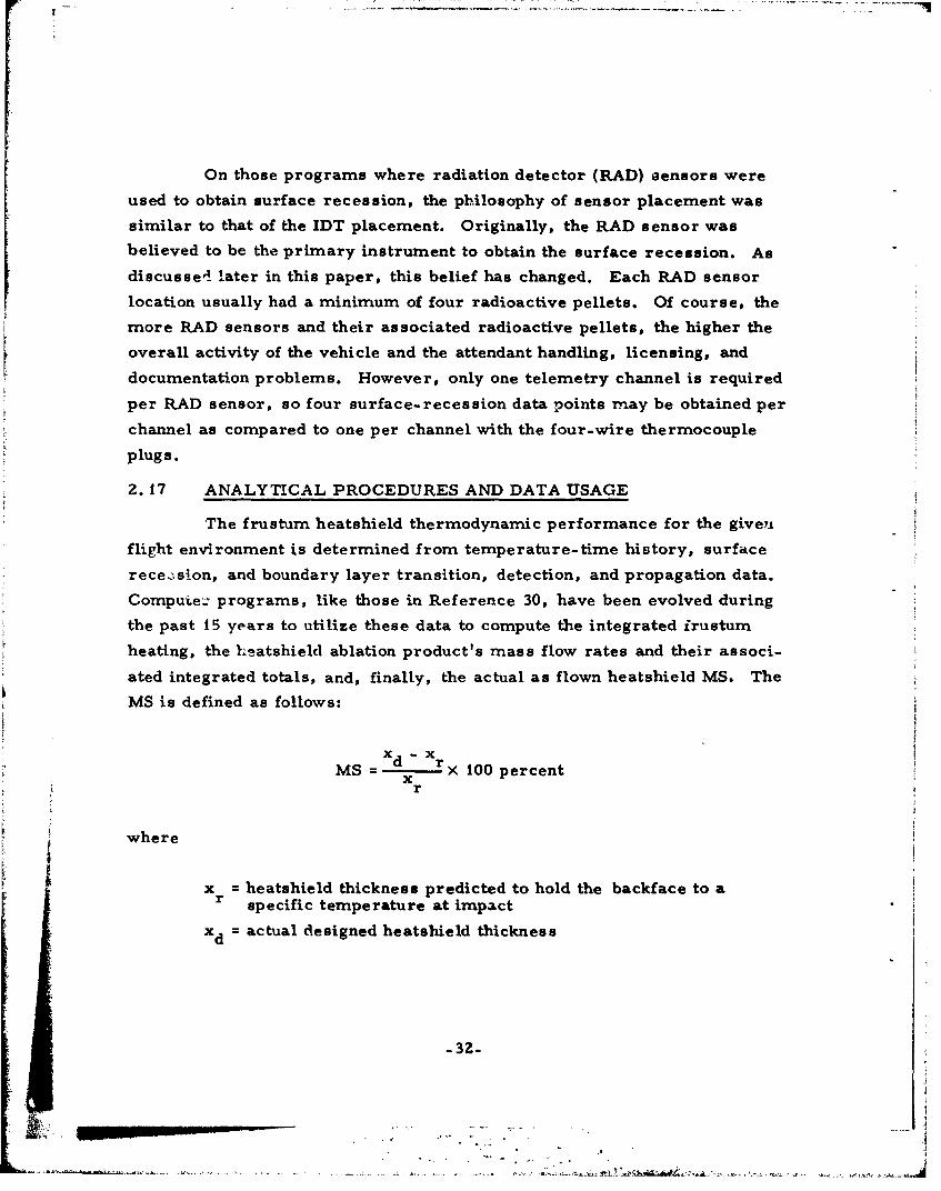
2.17 ANALYTICAL PROCEDURES AND DATA USAGE
The frustum heatshield thermodynamic performance for the given
flight environment is determined from temperature-time history, surface
rece-sion, and boundary layer transition, detection, and propagation data.
Compuie:" programs, like those in Reference 30, have been evolved during
the past 15 years to utilize these data to compute the integrated irustum
heating, the heatshield ablation product's mass flow rates and their associ-
ated integrated totals, and, finally, the actual as flown heatshield MS. The
MS is defined as follows:
x -xMS = 1r 100 percent
x r
where
x = heatshield thickness predicted to hold the backface to aspecific temperature at impact
xd = actual designed heatshield thickness
-3Z-
• . h.oj'~ . .
In general, the more predictable a heatshield material's performance
the lower the MS required. The specified MS for the SAMSO vehicles varies
between 25 and 50 percent, depending on the confidence in the known data of
the specific material prior to flight.
The thermodynamic performance of a frustum heatahield is evaluatedfrom a thermodynamic simulation of the heatshield. Several key inputs are
required for this simulation:
a. The actual trajectory flown by the reentry vehicle
b. The thermodynamic and thermochemical propertiesof the heatshield material
c. The onset, propagation, and nature of the laminar to.turbulent flow transition of the boundary layer
The flight trajectory is reconstructed from flight data, and the heat-
shield material properties are usually known prior to flight, although the
flight test data are occasionally used to determine some of these material
properties. It is necessary to know the location of the onset and progression
of transition (both axially and azimuthally over the vehicle) and the nature
f f the transition in order to properly program the postflight simulation.
For example, if transition occurs instantaneously at a point on the heatshield
the aerodynamic heating calculated up to that time will be a laminar heating
calculation, and the aerodynamic heating calculated after that time will be a
turbulent heating calculation. If, on the other hand, the transition is not
instantaneous, a laminar to turbulent transition relationship will be used to
c- !culate the aerodynamic heating. It is imperative that the aerodynamic
hating be simulated correctly because the accuracy of the entire postf~ight
slysis depends on that of the aerodynamic heating. Finally, when the post-
flight temperature-time and surface-recession-time histories are calculated,
they are compared to those measured in flight to assess the performance
of the heatshield and to aid in the diagnosis of flight anomalies.
-33-
• - •,.
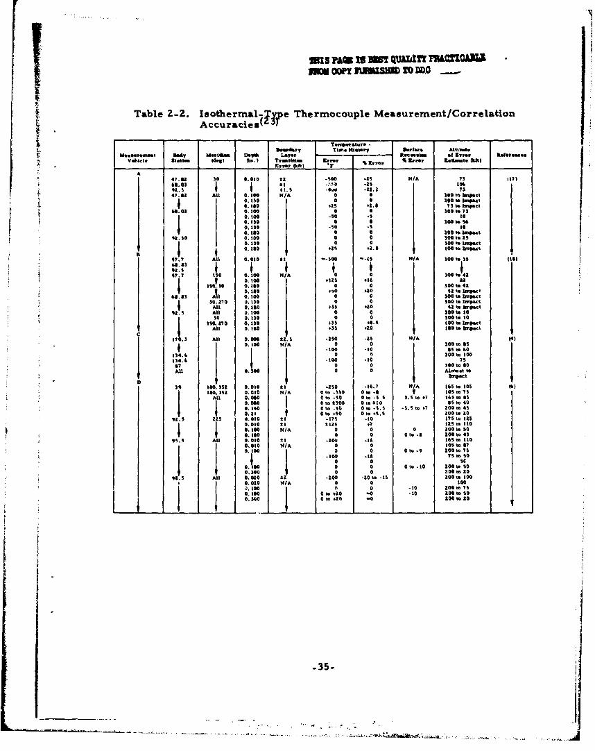
The isothermal-type thermocouple was used extensively on SAMSO
flight test programs to measure the onset of boundary layer transition,
heatshield temperature-time histories, and heatshield surface recession.
The estimated measurement accuracies attained by the isothermal-type
thermocouple are tabulated in Table 2-2 for representative vehicles from
those programs.
In Table 2-2, the correlation of surface recession as predicted by
postflight analysis to that measured in flight is expressed in terms of per-
cent for vehicle D. These data show, for example, that the predicted and
measured surface recession data compare to within -3.5 to +7 percent of
total recession of each other, where the flight test data were derived from
the temperature-time history data measured at station 39. At station 92. 5,
these flight and predicted data correlated from 0 to -8 percent in total
recession, depending on the meridian. Back at stations 95. 5 and 98. 5, the
correlation comparison falls off to -10 percent of the total recession.
Therefore, for vehicles equipped with the proper isothermal-type thermo-
couple plugs, the surface recession can be deduced from the temperature-
time history to within 10 percent of the total recession, ard these results
were comparable to those obtained by the RAD sensor installed at the same
stations.
The correlation of the temperature-time histories, as predicted
by postflight analysis, to that measured in flight is presented in Table 2-2
in terms of the difference between the two temperature-time histories in
degrees Fahrenheit and percentage error over the altitudes defined. The
latter is referenced to the predicted temperature-time history. For Vehicle A,
Table 2-2 shows that the flight test data correlated precisely with the pre-
dicted values for most of the trajectory. There were a few of the sensors
(130 mils or deeper into the heatshield) that deviated from -5 to +2.8 per-
cent from the predicted values. All of the 10-mil near surface thermocouples
-34-
SRIS PAQK IS lJ QWZALI' 'ti'iah3L= oon rtNiSHM 1zo DDO
Table 2-2. Isothermal- Tye Thermocouple Measurement/Correlationi Accuracies(13f
.trdy Tim. Htetory Sorfte.. Alt adoSM..omo.*t tgLy Mettlmef Dowt& Lyver Rau•reoeI of "r.r ItoforeuesSVehicle Sstaion (de8) (in,.) Treasitn Errr S E'rror S1 Error C~olinuto 01fti)
xr tor, (tft) "A
91. 1 e. t . S -.5 -22S. r 7347. U All 0.100 ±2 0 0 NA00 to lmuct
4 75 O. 0 0 0 WO to Imeaqt
S.180. 0 43 4.5 73*0 to lqmct65.03 0.100 0 0 300 to ?7S01o)-5o -S to
Ato.o NA0 30060 Snc0.10 0 0 300 ft
9A13. so 0.0 0 0 300*t310. 10 .50 0 $ pg t
!0, t+QS +2.9 100 to hpec*t
525 V I4T + All 0. i0 tt1-0 -- OO -- as N/A Soo to 35 |)
S47.7 0 0.100 0/0 300 .ooo 420.100 o+IZ 4*6 32
SS 30 0.180 0 300 to 41SO• 0. IS0 .40 .`10 135. tno pct
65.53 Al 0,100 0 0 300 hoped30.,270 3. 130 0 0 300 to Inpact
All 0.140 +35 +20 42. to apectS All 0.100 0 0 3005.0t
A0 0.130 43 40 t00 to 0i. | S 7 Z0 0.13S0 +3S +B. 50 wO bnatoI,•
CAll 0. tO0 +3 5 +Z 0 100 to b -•,ct
.t .3 All 0.000 a" 3. -I30 -15 NIA (4)17.3 0.100 N/A 0 0 to3001.554 I -100 -o o0 I N60
134.6 00 to 300 100' 134.6 -100 -10 75I 7 0 3 00 to 90
An 0.300 0 0 Alwost w0D I
39 1S0. 353 0.010 *1 .2s0 .16.7 N/A 1635t 10t (6)190.352 0.010 N/A O to -130 0 to 5. V 1@5 to 75
AUl 0.00 0 to -50 0 to -S 5 S. S to +7 363 to siI0.0410 0 to 3100 0 to It0o 5 to 40
0,140 0 to -30 0 to -3. 5 -3.S to #T7 200 t5 430.11 0 to 0 SO 0 to +S.5 ZOO to Z4
qZS IS 0.0*0 3* -17S -10 17SL0 "15*I 0.0:0 tl tt2s +7 113 to 1100.1100 N/A 0 0 0 200 to 500.110 0 0 0 to -I 100 to 4S
95.5 All 0.010 31 -40, -16 165 to 100:01O N/A 0 0 105.87O.100 0 0 0.to 0 to .7
-too -t 5 to 500 0 SC
0 (to 0 0 0to -to 200to S0O0, 300 0 0 200 to .00. NO0 1 -300 -30 to -IS Z00 so 1000,020 NIA 0 0 100
(1 0 -10 Z00 to TS0.110 0 t 20 -0 .10 zo00 0 to 00300 0 to +2 0 2001020
-35-
~.t- ~ - ,
however, were up to 25 percent lower than predicted. Most of the
Vehicle B flight test data were similar to the Vehicle A data in that:
a. Near surface thermocouple sensors were 25 percentlower than predicted
b. Most of the in-depth thermocouples (100 to 180 mils)correlated precisely with the predicted for low altitude
c. Some of the 130- and 180-mil sensors deviated fromthe predicted values
Some of the deviations were as high as 20 percent. The correlation
of Vehicles C and D data followed the same pattern of accuracies as those on
Vehicles A and B. The one disturbing aspect common to all four vehicles
was the 25 percent low flight test measurement (relative to the predicted)
exhibited by the near surface thermocouples prior to boundary layer transi-
tion. There have been a number of discussions within the SAMSO community
about this and the reasons include:
a. The high altitude laminar heating prediction is incorrect.
b. The 5-mil thermocouple wires plus insulation representa significant heat sink when covered only by 10 mils ofheatshield.
If the first reason were true, then none of the deeper thermocouples
should have correlated. A detailed continuance of this accuracy study is
presented in Reference 31.
In summary, the Table 2-2 dwta indicate that the isothermal-type
thermocouple does yield a delivered accuracy better than ±5 percent of
achial value for most sensors over most of the trajectory. An example of
a correlation between the flight test and the calculated temperature-time
histories for a vehicle utilizing the isothermal-type thermocouple is pre-
sented in Figure 2-31. This correlation is nearly perfect during most of
the reentry time for the isothermal-type thermocouples located at 0.080,
0. 140, and 0. 2 1 in. below the heatshield surface.
_36-
5A.
le*11
-37-
it4
IL04
L4
.38
STATION STATION
0.00
SSTRUCTURE
Fiue2-3. Mosetip WIti angle 13ac~akce Thjerrmo0 0
OTICAL U A
36~ LOOST rf
Ift d%/
OCOAVOM ..Vww LC*Wpaw~/
SIDWALL UIACKFACESTAGNATION REGIONTH -- E(3
SACKFACE THERMOCOUPLES (3) N.10
A-AHIT NO- NO110509
50dnNO. 110950dg NO- 11W9
270 dog
Figure 2-5. Graphite ShellNO.ei I akac Tepeatr
q0 THERMOCOUPL NO. 1104
150 ~ ~ THRMCOPL NO 10 0%N. 1105 .
10 ~ ~ 9 TIEs
Figure 2-5. Stagnatio Rhegi onei Backface Temperature Rsos
Instrumnta 40o
LEGEND:___
-CMPTE CALCUATION
Al 33 1Al A39
Al136 Al A38SECONDARY -Al 312 A142 , BALLAST iNOSETIP-
1•j .44PRIMARYAIN564--SAIO 33
A148 Al A43
STATION 2. 06 S 5.64'A13
STATION 0.00-' STATION 4.24- STATION 13.82
STATION:N.5 K.65 2 TION 1.3STATION 7.04- STATION 12.80
STATION 7.70-- I -STATION 10.60STATION 9. 50 180 €lma
90 dog - •--2T0 deg
0 dogVIEW LOOKING FORWARD
Figure 2-7. Nosetip With In-Depth Temperature Measurements
-41-
U.A-
- A147 42
93.8 .
STATION 4.24 A1?-17.8 -- .STATION 5. 64 A 413 2 i0A 140
STATION. 4.04 93-1.0 2w0 ~
w-17.8 0L-.ý
93.1 2w-1 I..- 0
368 369 370 3?1 372 37 34 375 376 3?7TIME AFTER LIFTOFF, s8c
Figure Z-8. Nosetip In-Depth Temperature Data
PLUG MADE OF SAME MATERIALAS HEATSHIELD
BREAKWIRES EMBEDDED INHEAT3HIELD PLUG
II
Figure Z-9. Breakwlre Ablation Sensor
d -42-
MOLYBDENUM COAT
NOSETIP SECONDARYNOSETIP
SEEDANT SECONDARY NOSETIPEC 22164E ANlINDIUM __SULPHIDEYTTERBIUMCARBONATE
Figure Z-10. Nosetip Instrumented With Seedante
GEIGER-MUELLER o p o ~ o
SOURCES
Figure Z-11. Radiation Transduicer Sensor Block Diagram
L -43-
:VI
S~11J
ii
DEPTHSOURCE in. cm
A 0.050 0.127B 0.288 0.732C 0.692 1.176
4.55 7.35 11.6 14.0 16.5 cm AFT OF TIP D 0.923 2.34
A BC D E
PRIMARY NOSETIP MATERIAL-o.- STRUCTURE
0.127 0.635 6.35 10.8 16.0 cm AFT OF TIP
Figure Z-1Z. RAT Installation
5 .
-- - t---* .-. .
u ItuI-lo
C -44
100
'OUMVN~ ' NOI II3N3 VI
I n "w jx Imm WI 141
-45-0
SCINTILLATOR4
MUL TIPL IERi PHIOTOUSE
SHNIELD
SUPPLY
MATER IAL
S11*AL DT
TIONILIN
Figure 2-15. BRAG Sensor Block Diagram
TIP MATERIALCOLLIMATION
PHOTOMULTIPLIERt
Figure 2-16. None Assembly With BRAG Sensor
-46-
O
5.W 2.0 0000
01
3.i1 1.5
i hLEGENO:
hi hi 0 BRAG SHNSORFLIGHT TEST DATA
1. •-PREFLIGHT PREDICTION 0
0 010 5 10 Is 20 25 30 35
TIME FROM 3w kft. see
Figure 2-17. Nose Stagnation Point Recession - BRAG
0 .0~m mA bil
TYPICAL.
BLACK GLASS TYPICAL 16 pc:.)-TYPICAL
QUARTZ CHROMIUM COATING INTERMEDIATEENTIRE TOP AND NOES. ADLATIONTYPICAL IT plemg) "
-- POLISHED OPTICAL INTERFACESIN INTIMATE COHTACT rno lpeY|"TYPICAL 17 plems)
La 1~'. 1"AtS F"[email protected] AL I? plow) PIPE NIL.I
0. IS DIAMfTER
9 - MTVILt NRS TTING. E VALENT
Figure 2-18. Light Pipe Ablation Sensor and Installation
-47-
TOP ONAA STIP T
MUT W REGTHERMOCOUPLR PLUG .-(45QIESS d"n m'd 21 dm51 -M PEPU
Figure 2-1. Light PiEMIsrmne oei
lUd " EI'TAN
10-d"n MERIDIAN
5.0 - 2 4
-48-4
-.20 ILP
MOLTEN O'!AItTZ FILM•.}• CCONDUCTIVE EPOXY
S PLTINUM
WIRE WITH
RESISTIVE 'ELEMENT
Figure Z-21. ARAD Sensor Design
R, - SENSOR RESISTANCER? = CURRENT SOURCE RESISTANCE
RQ1 ' R 02 a QUARTZ RESISTANCE
v INNER CONDUCTOR
+5V
SENSOR
R0
OUTER CONDUCTOR
Figure Z-ZZ. ARAD Schematic
-49-
- - -.- -- _-
LO16.0
14.0 ++
.2.0 AM>AMP -=+ :OSTI
Fius m-5 Nosi Acusi Intumnato
PLUG MADE OFSAM MATERI ALAS THEHEATSHIELD
WIRE COILEMBEDDEDIN THEHEATSHIELDPLUG
COMMONWIRE
Figure 2-26. Makewire Gage
THERMOCOUPLEASSEMBLY HEATSHIELD
STRUCTURE
Figure Z-Z7. Post-Type Thermocouple Install-aon
~5Z -
THEMOCOUPLECENTER PLUG ASSEMSLY
SLEEVE HEATSHIELD
f"//
SHIELDED PAIRSSTUUR
Figure 2-28. leothermal-Type Thermocouple Installation
TELEMETRY
SYSTEM
10 WTS< UNTW UNCTION lamP
Figure Z-29. Typical Measurement System
-S3-
STATION 61.8 "/.5 90.5S/R 6.7 15.8 21.0 2.O ag
PLUG IN $HELL 150 d9g 30
THERMOCOUPLE DEPTHS, mils
JUNCTION -30, 150. 270 digJUNCTION No. No. S/R
S8.7 15.6 21.0
1 20 10 102 150 100 1003 200 200 200
4 300 300 300
Figure 2-30. Frustum Shell Thermal Instru~mentation
5S 1 I | I I ! I ,- ANALYTICAL
5000 FLIGHT TEST DATA
0o FLIGHT TEST DATA
FLIGHT TEST DATA
IL. SURFACE--,- 0 0
3500 0.010 In. 0.080 In.S~O J40 In..
53000 010 n 0. 21 In.
200-i 0
13500- 0o
8000
1500
1000-
S0 a 4 6 I8 10 12 14 16 18
REENTRY TIME, sec
Figure 2-31. Isothermal-Type ThermocoupleTemperature -Time Histcry
-54-
"- i:. . ..... ...' -... ... • . .. ... ..... ...... . .. ...I-~-.-.~--------.-- .---- .-.
- - - - - - - -
3. AERODYNAMIC AND VEHIC LE
DYNAMIC INS TRUJMENTATION
3.1 PURPOSE /INTRODUCTION
RV flight test programs require extensive on-board instrumentation
in order to obtain aerodynamic and vehicle dynamic data with which to
evaluate RV performance. Flight data represent the "real world" and are
the only means by which reentry vehicle design parameters (maximum
loads or maximum heating) can be validated. In addition, the phenom'enology
of specific technology areas, or "fixes, " to a particular problem that cannot
be simulated in ground test facilities can be fully evaluated during flight
tests with the proper instrumentation. Obviously, flight instrumentation
that are reliable, accurate, and inexpensive are needed to obtain the
required data.
The most importanit aerodynamic and flight dynamic data. that are
generally obtained during a flight prog~am. are:
a. Drag characteristics (total and components)
b. Roll performance
C. Angle of attack
d. Stability
e. Aerodynamic force and moment coefficients
f. Axial and lateral loads
g. Transition onset altitude
These typical performance parameters require evaluation for the
R&D flight condition flown so that modeling techniques can be validated in
order to make accurate predictions for extrapolation over the entire RV V-y
map, including design conditions. A typical RV V -y map showing the entryconditions that the RV must be able to perform adequately, RV design condi-
ticon, and a typical R&D flight test matrix are shown in Figure 3-1.
-55-
The following section will deal with the required flight instrumenta-tion needed to obtain the necessary technology data to meet the RV mission
requirements. It should be noted that all of the instruments described,
photographs shown, and typical data are based on ballistic RVs. The in-
strumnentation, however, is directly applicable to maneuvering RVs.
3.2 FLIGHT INSTRUMENTATION PRINCIPLES
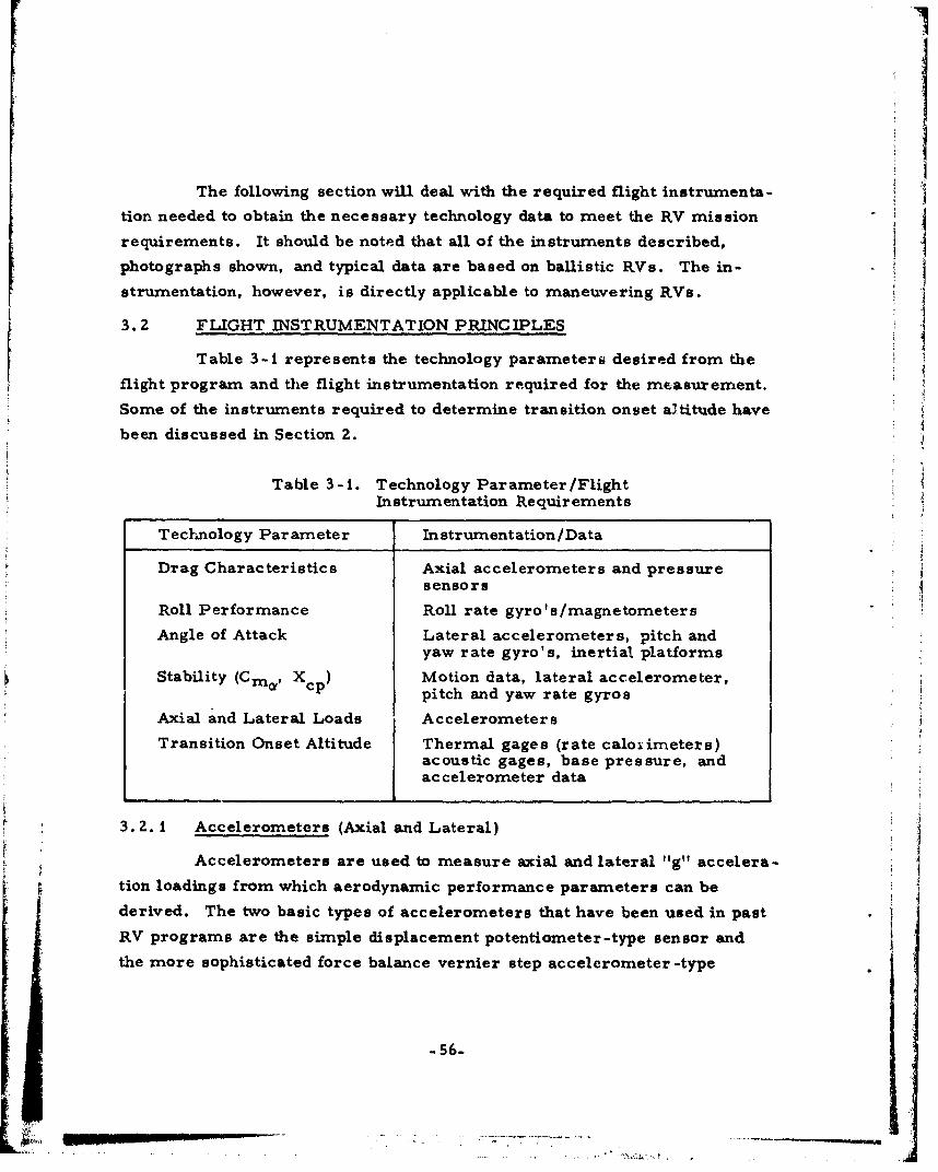
Table 3-i represents the technology parameters desired from the
flight program and the flight instrumentation required for the measurement.
Some of the instruments required to determine transition onset altitude have
been discussed in Section 2.
Table 3-i. Technology Parameter /FlightInstrumentation Requirements
Technology Parameter Instrumentation/ Data
Drag Characteristics Axial accelerometer s and pressuresensors
Roll Performance Roll rate gyro's /magnetometers
Angle of Attack Lateral accelerometers, pitch andyaw rate gyro's, inertial platforms
Stability (Cmc, X ) Motion data, lateral accelerometer,cp pitch and yaw rate gyros
Axial and Lateral Loads Accelerometers
acoustic gages, base pressure, and
______________________I accelerometer data
3.2.A Accelerometers (Axial and Lateral)
Accelerometers are used to measure axial and lateral 11g1 accelera-
tion loadings from which aerodynamic performance parameters can be
derived. The two basic types of accelerometers that have been used in past
RV programs are the simple displacement potentiometer -type sensor andthe more sophisticated force balance vernier step accelerometer -type -
-56-
. .... ........
sensor. Figure 3-2 shows a schematic of the displacement-type accelerom-
eter that consists of a seismic mass, a spring, and a dash pot damper. The
readout of this type of sensor is generally made by a potentiometer voltageI
divider. Figure 3-2 also shows a schematic of the accelerometer with
acceleration applied and the sensor at zero gs.
The potentiometer displacement accelerometer has been the most
commonly used on RV flight programs during the past decade. When these
sensors are used in axial load measurements (basically to derive the drag),
they are usually employed in overlapping ranges such as 0 to 5 g's, 0 to 20
' is, 0 to 40 g's, and 0 to 100 g's. The above sensor ranges provide total
drag measurements from '-140 kft to impact and, of course, cover the flow
regimes from laminar, transitional, and turbulent flow. The displacement
accelerometer is relatively inexpensive and rugged, but it has limited
resolution and accuracy due to the fact that the output is governed by a
wiper arm/potentiometer mechanism that is proportional to the "g" loads
as previously discussed. A typical analog trace of a coarse range (0 to 100
g'Is) displacement potentiometer -type accelerometer is shown on Figure 3 -3for axial loads.
A second type of accelerometer hxi use is the force balance accel-
erometer. This type of accel.erometer also employs a seismic mass Similar
to the displacement -type accelerometer. However, the force balance accel-
erometer has a constrained seismic mass and senses a slight displacement
due to acceleration in the sensitive plane. The amount of force required
for constraint (force balance) to restore the seismic mass to the null posi-
tion is proportioi.al to the acceleration applied. The null position is generally
measured by an inductive coil and an amplified signal as shown in Figure 3-4.
The force balance accelerometer is significantly more accurate and has
infinite resolution. These features provide the opportunity for two major
innovations. The first is the duaal-range accelerometer, which is simnply a
force balance accelerometer with one sensing unit having a dual output
consisting of two amplified levels (Figure 3-5). A typical dual-range
............ ........... .....-.. I.a',cI,2A..iLa..,.kn *
accelerometer, which is cu:1-rently being flown on RVs, has a range of ±t3 g's
and ±30 g's. This sensor is being used to measure lateral loads in the pitch jand yaw planes.
The second innovation, the vernier step accelerometer, was de-
veloped because today's sophisticated technology for weapons systems RVs
requires highly accurate measurements. It has been successfully flown onsvrlflight programs. The vernier accelerometer has five basic ranges
in oe sinle instrument and is more accurate and has better resolution
than the pot-type displacement or the dual-range, force balance acceler-
ometer; however, the vernier accelerometer is significantly more expensive.
The vernier step accelerometer also operates on the force balance principle
and has five amplified levels operating off the same sensing element. This
instrument provides very accurate drag measurements. One channel pro -
vides a 0 to 5.0O-V full -scale output having ranges from +1, to -3, -2 to - 10,
-8 to -24, -20 to -52, and -44 to -108; a second output defines the range
at which the sensor is operating (Figure 3-6). This sensor is currently
being utilized to measure axial g's on RVs. A typical analog trace from a
vernier step accelerometer is shown in Figure 3-7. Axial accelerometer
data are utilized to determine the axial force coefficient (C ), which is the
major component of drag and will be discussed in Section 4.
Lateral accelerometers can be either the pot displacement or the
force balance typeand are used i overlapping ranges in the pitch and yw
planes of the RV. Typical pot sensor ranges are ±10 g's andi ±40 g's and
±100 g's or ±t3, ±30 g's for the dual-range force balance sensors. Lateral
accelerometers provide several important inputs to determine the RV
performance. These are-
a. Lateral loading
b. RV total angle -of -attack historyC. RV trim angle of attack
d. The presence of nosetip asymmetries
e. Normal force coefficient slope (C)
-58-
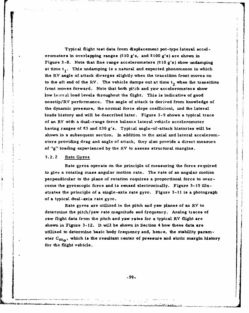
rTypical flight test data from displacement pot-type lateral accel-
* erometers in overlapping ranges (±10 g's, and ±100 g1s) are shown in
Figure 3-8. Note that fine range accelerometers (±10 g's) show undamping
at time t This undamping is a natural and expected phenomenon in which
the RV angle of attack diverges slightly when the transition front moves on
to the aft end of the RV. The vehicle damps out at time t2 when the transition
front moves forward. Note that both pitch and yaw accelerometers show
low laeral load levels throughout the flight. This is indicative of good
nosetip/RV performance. The angle of attack is derived from knowledge of
the dynamic pressure, the normal force slope coefficient, and the lateral
loads history and will be described later. Figure 3-9 shows a typical trace
of an RV with a dual-range force balance lateral vehicle accelerometer
having ranges of ±3 and ±30 g's. Typical angle-of-attack histories will be
shown in a subsequent section. In addition to the axial and lateral accelerom-
eters providing drag and angle of attack, they also provide a direct measure 4
of "g" loading experienced by the RV to assess structural margins.
3.2.2 Rate Gyros
Rate gyros operate on the principle of measuring the force required
to give a rotating mass angular motion rate. The rate of an angular motion
perpendicular to the plane of rotation requires a proportional force to over-
come the gyroscopic force and is sensed electronically. Figure 3-10 illu-
strates the principle of a single-axis rate gyro. Figure 3-11 is a photograph
of a typical dual-axis rate gyro.
Rate gyros are utilized in the pitch and yaw planes of an RV to
determine the pitch/yaw rate magnitude and frequency. Analog tzaces of
raw flight data from the pitch and yaw rates for a typical RV flight are
showvn in Figure 3-12. It will be shown in Section 4 how theme data are
utilized to determine basic body frequency and, hence, the stability param-
eter Cma, which is the resultant center of pressure and static margin history
for the flight vehicle.
-59-
Rate gyros are also utilized to measure the roll rate of an RV
during reentry. An analog trace of the roll rate history for a typical RY is
shown in Figure 3-13.
3.2.3 Magnetometers
A magnetomneter is an instrument that measures the intensity and
direction of magnetic forces. Magnetometers are utilized on RVs to mea-sure the roll rate and to determine direction of the axes in inertial space
relative to the earth for detailed trajectory reconstruction.
Figure 3-14 is a photograph of a typical flight unit. Raw flight data
from a magnetometer are presented in Figure 3-15. The data sh~ow an in-
crease in frequency during reentry due to the normal roll rate buildup.
-1-2.4 Inertial Platforms
Inertial platforms are sophisticated instruments that determine RV
altitude and angle-of -attack histories. However, these instruments are
bulky and expensive when compared to accelerometers and rate gyros that
can perform the same function with slightly less accuracy. Accelerometers
and rate gyros provide adequate flight data for most ballistic RVs. Inertial
platforms have been used on ballistic RVs where extreme accuracy is re-
quired or a detailed technology flight experimealt is being implemented.
However, the most common and ideal use for an inertial platform is on
maneuvering RVs. Inertial platforms are beyond the scope of this paper.
3.2.5 Pressure Sensors (Steady State)
(32)The majority of flight pressure sensors in use today rely on a
diaphragm or aneroid capsule to sense the pressure difference between the
pressure to be measured and a vacuum reference pressure. The pressure
differential causes a diaphragm to bend or flex and produces a diaphragm
* displacement proportional to the pressure applied to the sensor. Diaphragm
displacement can be sensed mechanically via a linkage, wiper arm, andpotentiometer similar to the "Pot" sensor shown in Figure 3-16. Another
-60-
1A _____________________________________________
way to sense diaphragm displacement is with strain gages (bonded, unbonded,or diffusion-deposited), which measure diaphragm displacement by resistance
bridge and the accompanying inbalance that is proportional to the pressure
applied. A typical solid state, strain gage pressure sensor is shown in
Figure 3-17. These sensors are generally utilized to measure RV forebody
and base pressure data having a range from 0 to 5 psia to 0 to 100 psia.
Typical forebody flight test pressure data using a solid state strain gage are
presented in Figure 3-18.
A final way to determine diaphragm displacement is by variations
in capacitive or inductive coupling; this technique is generally employed on
low range pressure sensors, which are more sensitive, tend to be larger,
and are used to detect transition onset from base pressure measurements.
These sensors have ranges from 0 to 0. 1 psia to 0 to 5. 0 psia and
rely on the capacitance or reluctance principle. Figure 3-19 shows a photo-
graph of a low range, 0- to 0. 5-psia, variable capacitance pressure sensor.
Figure 3-20 shows low range, raw base pressure data for a typical RV
flight test. Figure 3-21 shows raw flight test data from a high range,
0- to 5-psia sensor used to determine the base drag component of total drag.
Section 4 will deal with the utilization of pressure data to obtain
the drag components of total drag for definition of the aerodynamic perfor-
mance of an RV.
. .
-61-
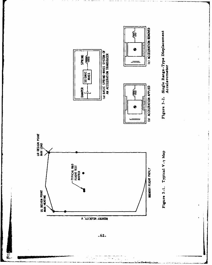
T 9
CL.
4bo
-IAo
Ii -
Lo q-
D IL
A -A103 ASM33
-62- I
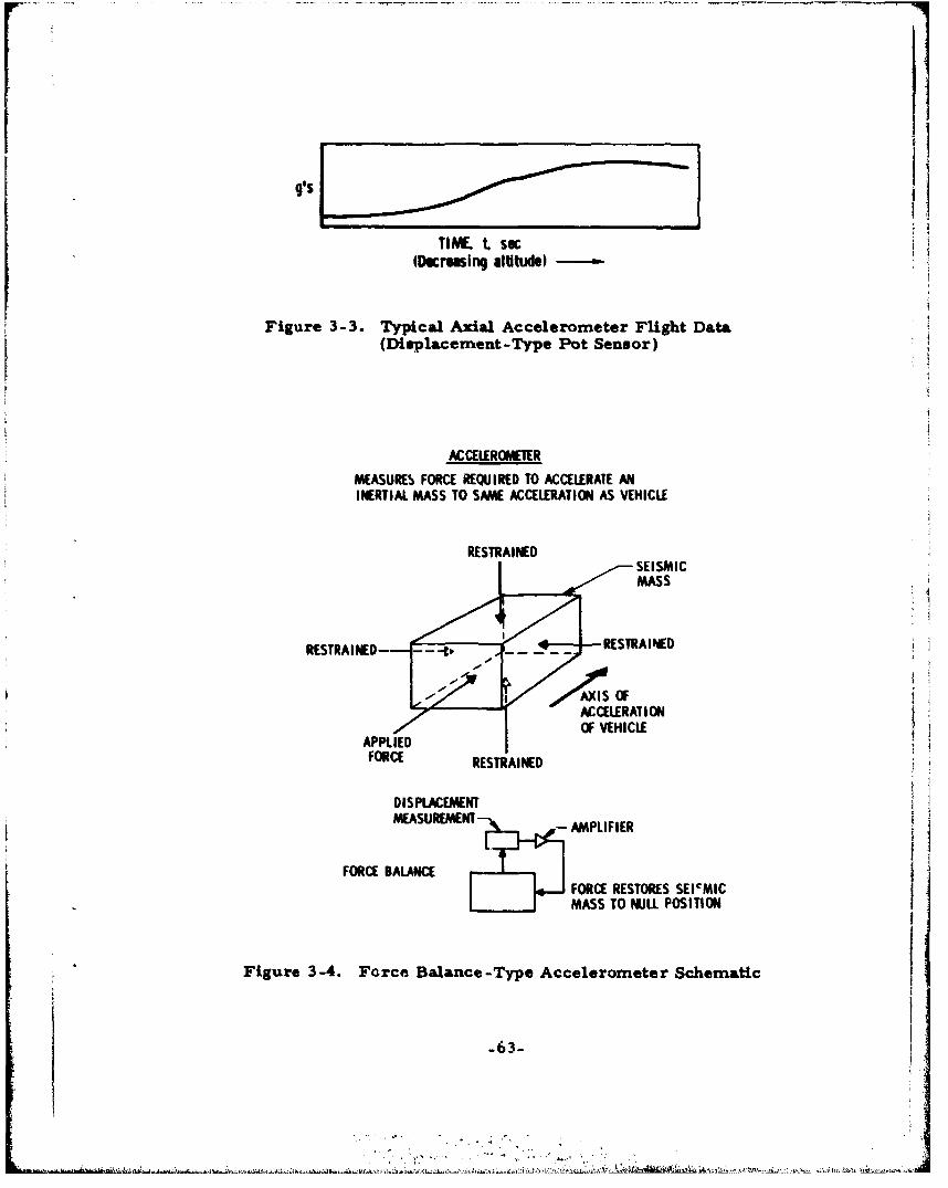
ges
TIME. t sac(Decresing altitude)
Figure 3-3. Typical Axial Accelerometer Flight Data(Displacement-Type Pot Sensor)
ACCELEROMETER
MEASURES FORCE REQUIRED TO ACCELERATE ANINERTIAL MASS TO SAME ACCELERATION AS VEHICLE
RESTRAINEDSE I SM ICMASS
AIS OFACCELERATION '
/ ~OF VEHICLE
FORRESTRAINED-TR-
DISPLACEMENTMEASUREMENT - AMPLIFIER
FORCE BALANCE T IFORCE RESTORES SEIeMICMASS TO NULL POSITION
Figure 3-4. Force Balance-Type Accelerometer Schematic
-63-
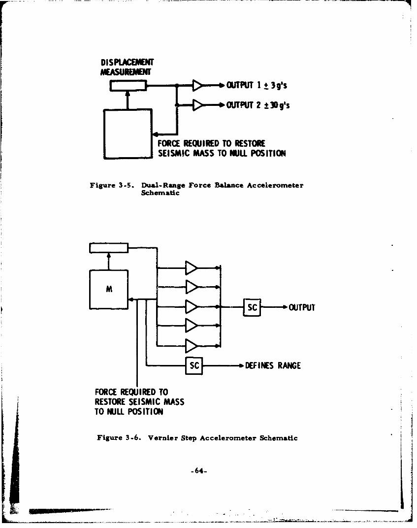
DISPLACEMENT
OUTPUT 1 ± 3g9s
p ~OUTPUT 2 ± 30 9's
HFORCE REQU IRED TO RESTORESEISMIC MASS TO NULL POSITION
Figure 3-S. Dual-Range Force Balance AccelerometerSchematic
SC eDEFINES RANGE
FORCE REQUIRED TORESTORE SEISMIC MASSTO NUJLL POISITION
Figure 3-6. Vernier Step Accelerometer Schematic
_64-
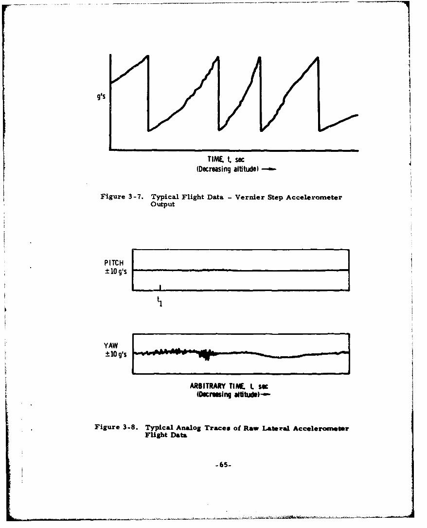
I1
g's
TIME, t. sec(Decreasing altitude)
Figure 3-7. Typical Flight Data - Vernier Step AccelerometerOutput
PITCH10 q's
ti
YAW±10 g's
ARBITRARY TINE. . sac-(Iecrmsing aftitudb-a-
Figure 3-8. Typical Analog Traces of Raw Lateral AccelerometerFlight Data
-65-
- i..j,. t LJ5JsY i.{i S
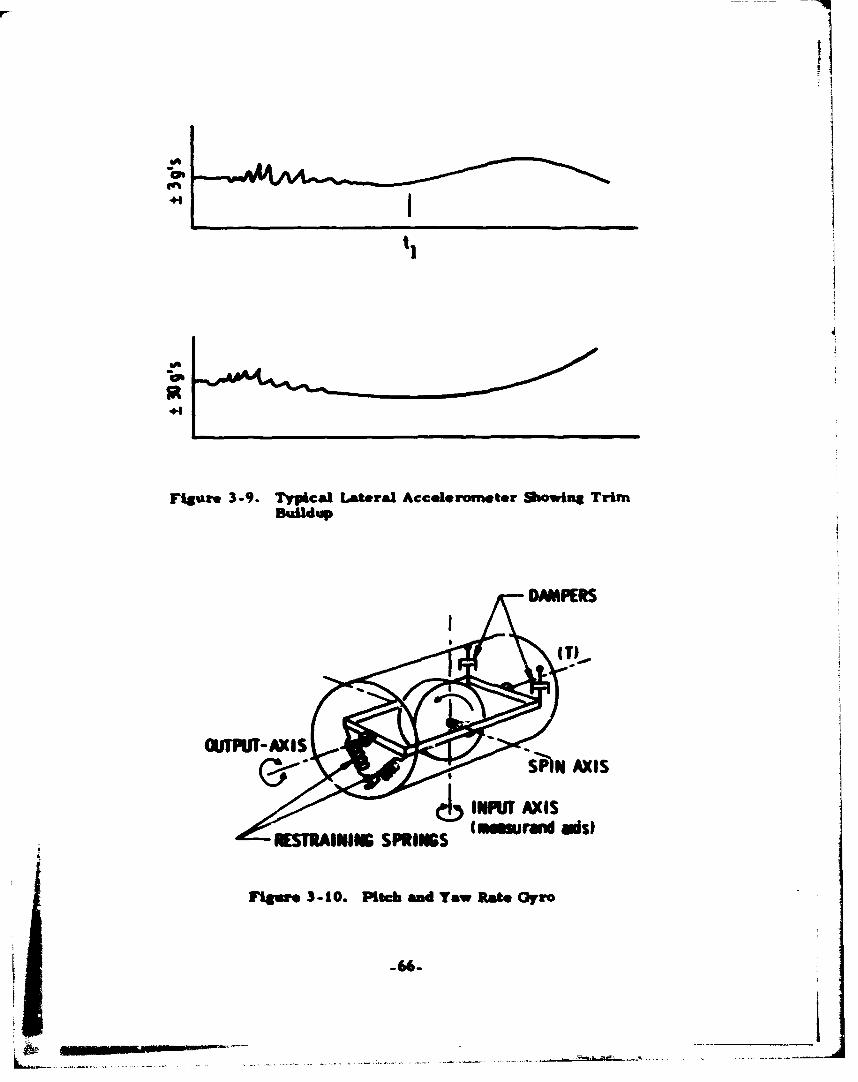
ti
st
Figawm 3-9. Typical Lateral Acceleronwter abowiug TrimBuildup
ESRININGS SPRINGSI aumlds
rigor* 3-10. Pitch and Taw Rate Gyro
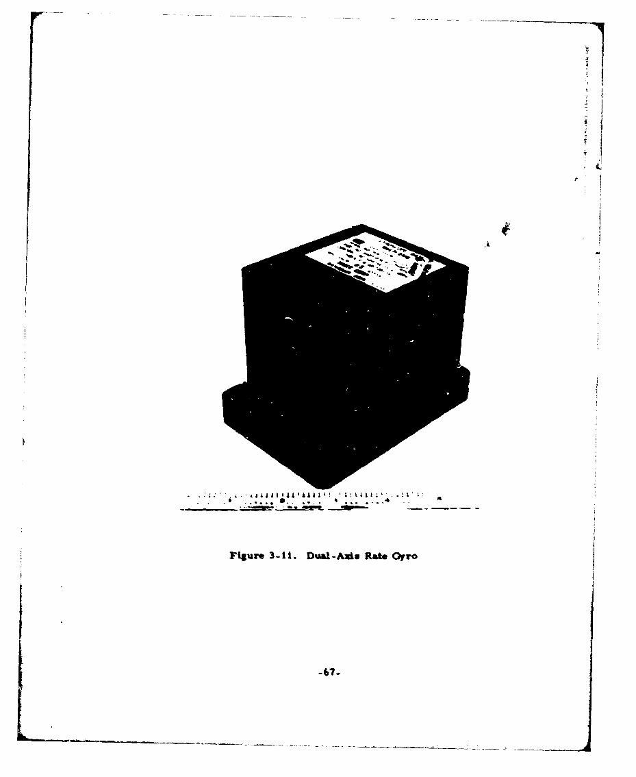
Figure 3-11. DuAk-Aads Rate Gyro
-67-
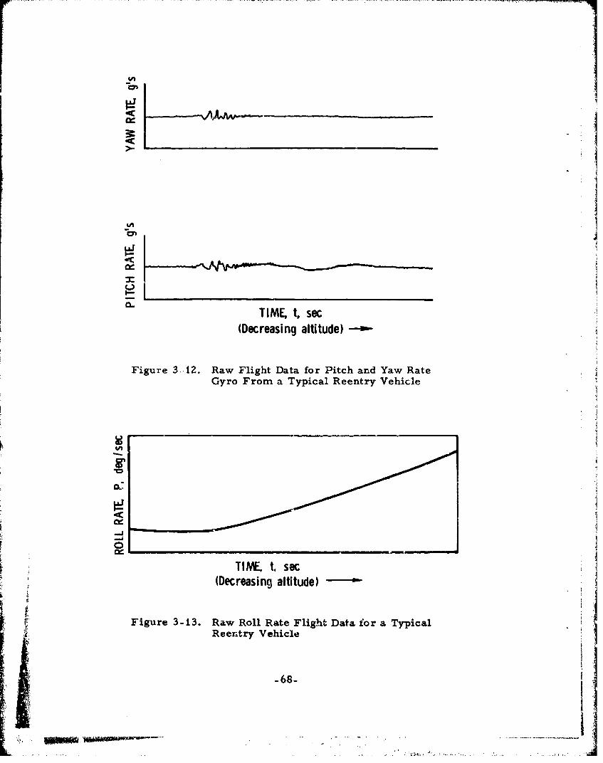
i/I
C-)r.n
TIME, t, sec(Decreasing altitude)
Figure 3. 12. Raw Flight Data for Pitch and Yaw RateGyro From a Typical Reentry Vehicle
.-,
TINE t, sac(Decreasing altitude)
Figure 3-13. Raw Roll Rate Flight Data for a Typicalk Reentry Vehicle
-68-
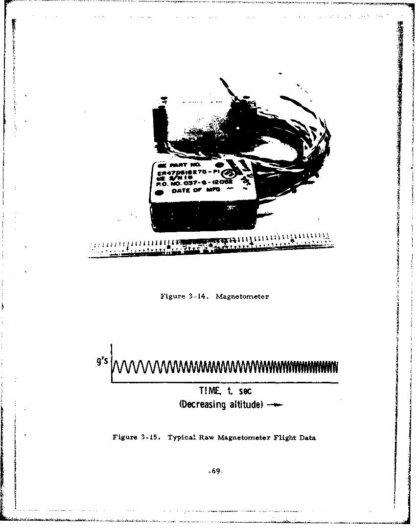
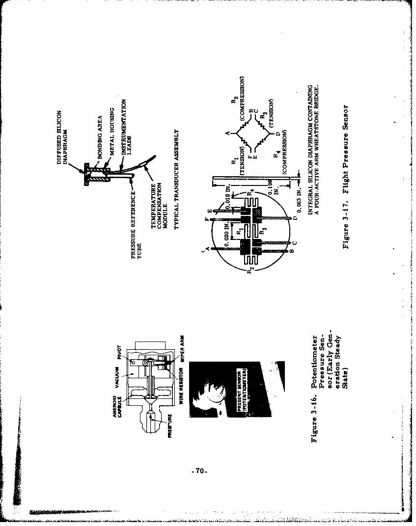
0 .
F-4)
0 P4
v-4
0 a4
Q0
0 II
IEI
-70-
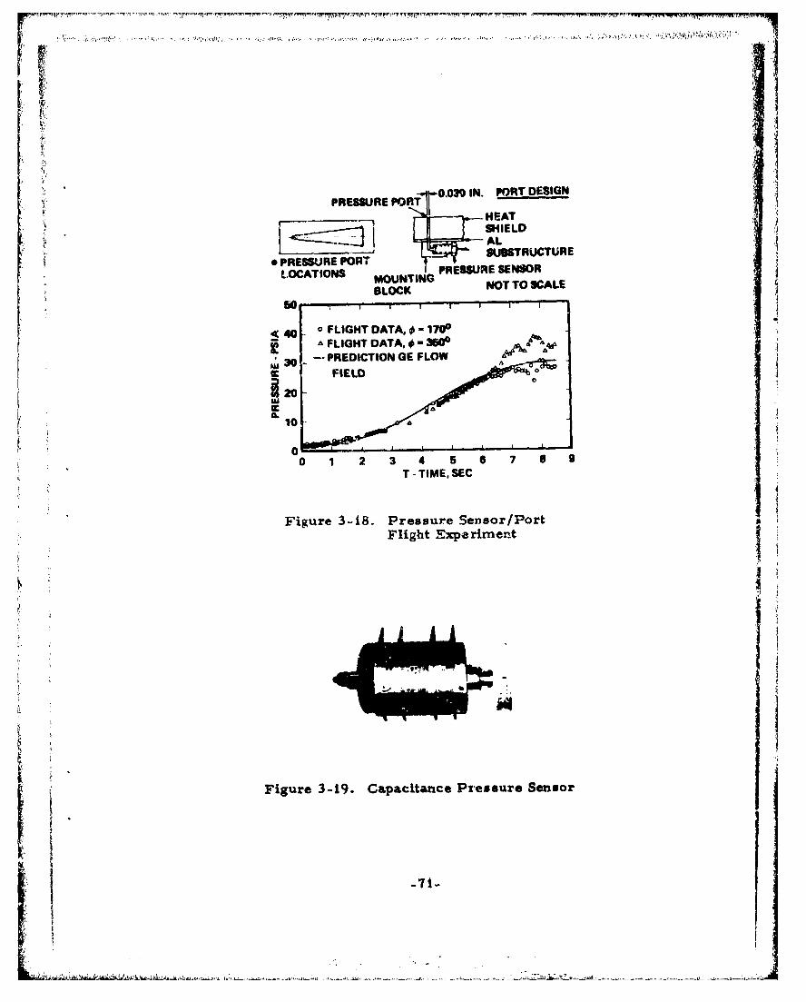
•.r
0 F•R-..0030 IN. PORT DESIGNPRESSURE PORT
AFU DATA ------OHEAT
PESR PORITLOCATIONS NMOUNTINGPESRESNO
BLOCK NOT TO SCALE
I I
<40 - o FLIGHT DATA, " 17&°
FLIGHT DATA. P e- 3 Sno r/Poi30 -" PREDICTION GE FLOW• 0 FED "•-
FIEL 0 0
120-
LE
'• Figure 3-18. Pressure Sensor/Port:, ~ Flight Expe riment
Figure 3-19. Capacitance Pressure Sensor
I- . -l• ,•. • • ,• • .... ... .• .............. ..... ,•-.71-. 2 . ... . .
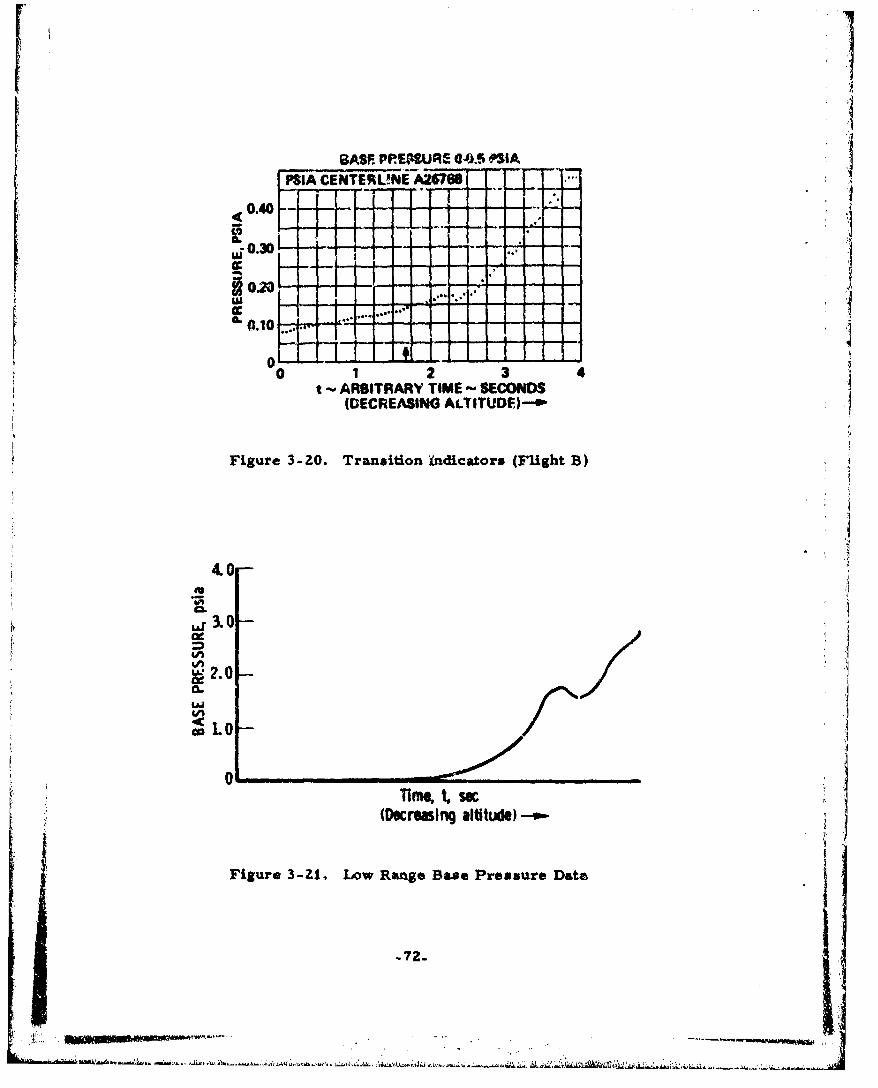
8ASE PPEPSJRE 0O., OSIA IPSIA CENTERLUNEA276
0.40
0.300 -
w o o- I ..... . '- -' -
I. 0.10 . 1----....L 0
0 1 2 3 4
t -- ARBITRARY TIME SECONDS(DECREASING ALTITUDO)--
Figure 3-20. Transition indicators (Flight B)
4.0
CA 2r.0 -
CI 1. 0 S=OLo
_ ii i ., ,, m ,, .Tim e t. sa
,I (Decreasing altitude) --
Figure 3-41. Low Range Base Pressure Data
-_72-- -. ,~.
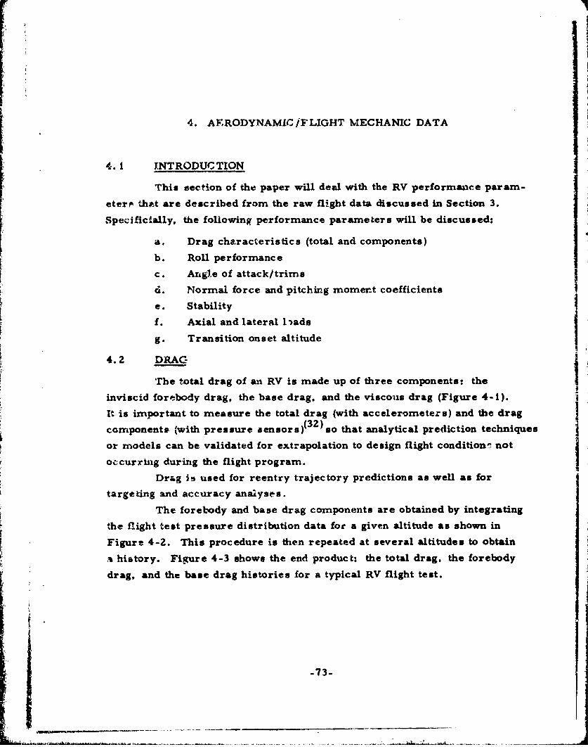
4. AFRODYNAMIC /FLIGHT MECHANIC DATA
4.1 INTRODUCTION
This section of the paper will deal with the RV performance param-
eterr. tha are described from the raw flight data discussed in Section 3.
Specificially, the following performance parameters will be discussed:
A. Drag characteristics (total and components)
b. Roll performance
c. Angle of attack/trims
d. Normal force and pitching moment coefficients Ie. Stability
f. Axial and lateral lIads
g. Transition onset altitude
4.2 DRAG
rhe total drag of an RV is made up of three components: the
inviscid forebody drag, the base drag, and the viscous drag (Figure 4-1).
It is important to measure the total drag (with accelerometers) and the drag
component* (with pressure aensors)(3 2 ) so that analytical prediction techniques
or models can be validated for extrapolation to design flight conditionr' not
occurring during the flight program.
Drag i5 used for reentry trajectory predictions as well as for
targeting and accuracy analyses.
The forebody and base drag components are obtained by integrating
the flight test pressure distribution data for a given altitude as shown in
Figure 4-2. This procedure is then repeated at several altitudes to obtain
ahistory. Figure 4-3 shows the end product: the total drag, the forebody
drag, and the base drag histories for a typical RV flight test.
-73-
4.3 ROLL PERFORMANCE
It is important to be able to determine the roll performance of an
RV so that a statistical data base can be established for the class of heat-
shield for modeling purposes. It has been established that roll torque on an
RV is a strong function of heatshield tape-lap splice orientation. If the
heatshield tape laps are all in one direction (++), the RV will tend to spin
up in that direction. Conversely, if part of the RV heatshield is ++ and
part is not, the vehicle will have a lower spin rate. Figure 4-4 shows typica l
roll rate flight data for RVs with different heatehield constructions. It is
important to control the roll rate within an optimized corridor for an RV via
passive means. Too high a roll rate will cause the vehicle to encounter roll
resonance with a resulting angle -of-attack divergence, high lateral loads, and
a range shortening and/or a decrease in accuracy.
Too low a roll rate may cause the vehicle to spin through zero,
which produces unacceptable targeting errors. Accordingly, it is important
to measure the roll rate for each flight and reduce the data to coefficient'4
form (C1 0 , roll torque coefficient) for phenomonology studies for extrapola-
tion to any V-V flight condition. Figure 4-5 shows the nondimensionalized
roll torque coefficient for several flight tests. Roll rate and roll torque
coefficients can also be obtained from magnetometer data and will be dis-
cussed in a subsequent section.
4.4 ANGLE OF ATTACK/TRIMS
The angle of attack or angle of trim can be obtained in two ways.
The simplest technique is .o utilize the resultant lateral g's in conjunction
with the predicted dynamic pressure and the normal coefficient slope. This
technique assumes linear aerodynamic coefficient and represents a fairly
_74-
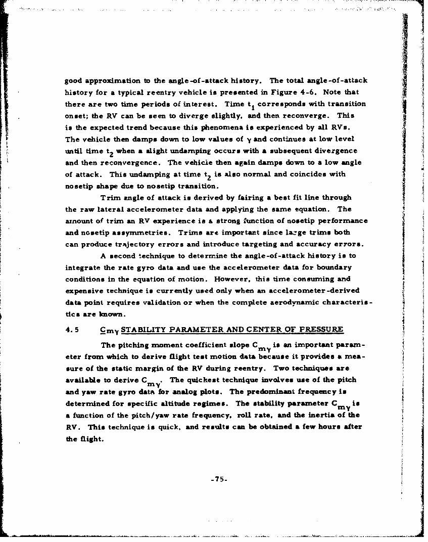
good approximation to the angle-of-attack history. The total angle-of-attack
history for a typical reentry vehicle is presented in Figure 4-6. Note that
there are two time periods of interest. Time t1 corresponds with transitiononset; the RV can be seen to diverge slightly, and then reconverge. Thisis the expected trend because this phenomena is experienced by all RVs.
The vehicle then damps down to low values of y and continues at low level
until time t2 when a slight undamping. occurs with a subsequent divergence
and then reconvergence. The vehicie then again damps down to a low angle
of attack. This undamping at time t2 is also normal and coincides withnosetip shape due to nosetip transition.
Trim angle of attack is derived by fairing a best fit line through
the raw lateral accelerometer data and applying the same equation. The
amount of trim an RV experience is a strong function of nosetip performance
and nosetip assynmuetries. Trims are important since large trims both
can produce trajectory errors and introduce targeting and accuracy errors.A second technique to deterrm'ine the angle-of-attack history is to
integrate the rate gyro data and use the accelerometer data for boundary 4
conditions in the equation of motion. However, this time consuming and A
expensive technique is currently used only when an accelerometer -derived
data point requires validation or when the complete aerodynamic characteris-
tics are known.
4.5 Cmy STABILITY PARAMETER AND CENTER OF PRESSURE
The pitching moment coefficient slope C is an important param-my
eter from which to derive flight test motion data because it provides a mea-
sure of the static margin of the RV during reentry. Two techniques are
available to derive Cmy. The quickest technique involves use of the pitch
and yaw rate gyro data for analog plots. The predominant frequency is
determined for specific altitude regimes. The stability parameter C is
a function of the pitch/yaw rate frequency, roll rate, and the inertia of the
RV. This technique is quick, and results can be obtained a few hours after
the flight.
-75-
A more sophisticated technique involves use of petal plots that
entail plotting the pitch rate ver sus the yaw rate for specific altitude
regimes. Figure 4-7 presents a petal plot for a typical flight %.et. The
intersection of a line from the origin to the edge of the ellipse represents
the C value. This technique is time consuming but is inherently moremyaccurate when used in a stability or center of pressure (X )assessment.cpFigure 4-8 presents a comparison of the C from a typical flight asmyderived from frequency and petal plot techniques.
The ultimate use of C is for a derivation of the static margin ormycenter of pressure location at specific points along the reentry trajectory.
Figure 4-9 presents a schematic showing the relative locations of the
center of gravity (CG) and X .p For adequate vehicle performance, the
CG of the RV must be forward of the X for the entire trajectory or thecpRV will become unstable. It is imperative that the X cpor the static margin(SM) be assessed for the RV flight program.
4.6 NORMAL FORCE AND PITCHING MOMENT COEFFICIENT.
It is imperative that the basic aerodynamic characteristics (drag,stability, normal force, and pitching moment coefficients) be derived from
flight data in order to validate modeling techniques that accurately predict
the vehicle trajectory parameters. Drag and stability have been discussedpreviously. This subsection will deal with the normal force and pitching
moment coefficients as a function of angle of attack. There are basicallythree steps involved in these microscopic analyses. First, specific altituderegimes of interest are selected where there are sufficient motion oscilla-
tions for the techniques to be valid. The angle -of -attack history is thenderived by integrating the pitchlyaw rate gyro data as described in sub-section 4.5S. Figure 4- 10 shows typical results. The second step io todetermine a history of the normal -force coefficient directly from the lateralaccelerometer data (G )
-76-
Figure 4-11 presents the time histories of the normal force and
pitching moment coefficients versus time. The third step is to cross-plot
these results with the angle-of-attack history to obtain the final aerodyna-
rmics (pitch angle-of-attack history) shown in Figure 4-12. This technique
also provides a bonus since the slope of the data (see dashed lines) will
yield additional independent data to confirm the stability and center of
pressure.
4.7 AXIAL AND LATERAL LOADS
The axial and lateral load& experienced are rather straightforward
and merely require patching together the various range sensors and apply-
ing the proper corrections for CG offset. Figure 4-13 presents a typical
axial and lateral load history.
Magnetometers can be utilized to measure both the roll rate of an
RV and the RV state vactor relative to the earth. Roll rate can be measured
with gyros: however, only the magnetometer can provide the direction of
the body axis and vehicle orientation in inertial space. These data are used
when microscopic analyses are performed for detailed trajectory recon-
struction to support accuracy and modeling assessments. Figure 4-14
presents typical magnetometer data.
4.8 CONCLUSIONS/FLIGHT DYNAMIC MNSTRUMENTATBON TRENDS
The detailed on-board flight instrumentation required for typical
reentry vehicles have been described. Several types of flight measurement
have been discussed to derive the same parameter. The purpose of this
paper has been to disseminate typical flight test data. to illustrate what the
data are used for. and to aiggest trends for future RVs. The basic aerody-
namic characteristics of an RV are:
a. Drag
b. Normal force and pitching moment coefficients
c. Roll rate
d. An*1e-Ot-attack characteristics
-77-
The foregoing characteristics can be obtained with a full comple-
ment of accelerometers, rate gyros, pressure senbors, and magnetometers.
The basic task of the flight test engineer is to utilize the most cost-effective
instrumentation consistent with the mission requirements. The following
guidelines represent recommended procedures for both RV technology flight
programs.
It has beeL shown that the vernier step force balance accelerometer
is far superior to the displacement pot-type accelerometer in terms of both
accuracy and resolution; therefore, it is the recommended type.
The dual-range, force balance lateral accelerometer is superior
to overlapping ranges of displacement pot-type accelerometers.
Low-range pressure measurements (P < 1. 0 pica) are best made
with capacitance -type sensors. High-range pressure measurements
(P = 5 to i00 psia) are best made with solid state, strain gage sensars.
The standard rate gyro is sufficient in its present form.
Roll rate can be obtained from a gyro or a magnetometer. It is
recommended that the magnetometer be utilized on research flight programs
as it provides both roll rate and the altitude of the RV in inertial space
relative to the earth for detailed trajectory reconstruction and accuracy
studies. However, the standard roll rate gyro would be more cost offectivv
for standard flights.
S-.78-
- -.--.-..-.-- . . --
0 TOTAL DR1AG
DRAG
K ~ WV3ICID PRESUUIE DRAG
TIM IL sm
]Figr* 4-I1. Typical Dr"g Conipoe Oaatbuildh*
4
II
STA a SlrA 2
TYPICAL FOREBOOY AXIAL
PRESSURE DISTRIBUTION (STEADY STATE) ooE SHOULDER FLIGHT TEST DATA
FLIGNT DATATANGEPKT POINT1FLO DAT 4
0 3SYM
FLIGHTDATA
U w 0
-GE FLOW
a." . 1 •FIELD SOLUTIONPREDICTED
EOUNIVALINT NIPE cow~:Sum
FLOW FIELDjEXACT UNABLATED SlAPE 0
6,111 FLOW FIELD J0. 0,4 O.6 0,11 1,0 0A 0 20 40 So so 100 120 140
X/L BODY ANGLE. - DEGREES
Figure 4-2. Flight Test Pressure Data
-80-
o TOTAL ORP4. AICELEMOUETER DATA
o - SAI DRAG. PREW1UE DATA
A FORESODY ODAG. rIESSURE DATA 0
0
0°00o00 o
Ea
h DECREASING ALTITUDE "•
Figure 4-3. Typical Flight Test Data -
Measured Drag Componentsvs Altitude
.•! I
•4200
HEATSHIELD 1
I I I , I , I , , _ ,
150 130 110 90 70 50 30 10
ALTITUDE, kft
6,60
V' 4200 - HEATSHIELD 2
100-I-Ix
150 130 110 90 10 50 30 10AITIUDE, kft
SFigure 4 4. Roll Rate vs Heatshield Type and Altitude
.82-
L ._27_. - - :rr '-- - . . ...
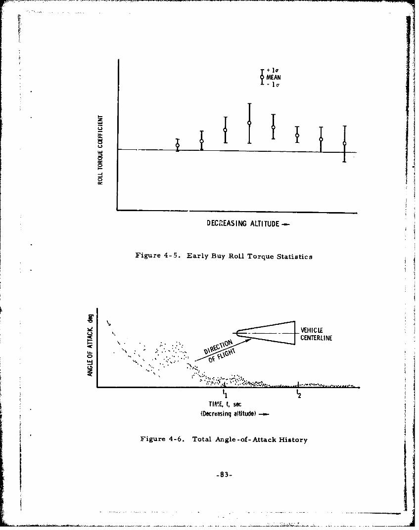
+1'1+ ~MEAN
- lc
oV
tt
DECMEASING ALTITUDE -,
Figure 4-5. Early Buy Roll Torque Statistics
_____ VEH I CLECENTERLINE
,L. . ."." : .".
ti t2TI•ME, t, sec
(Decreasing altitude) ---
Figure 4-6. Total Angle-of-Attack History
-83-
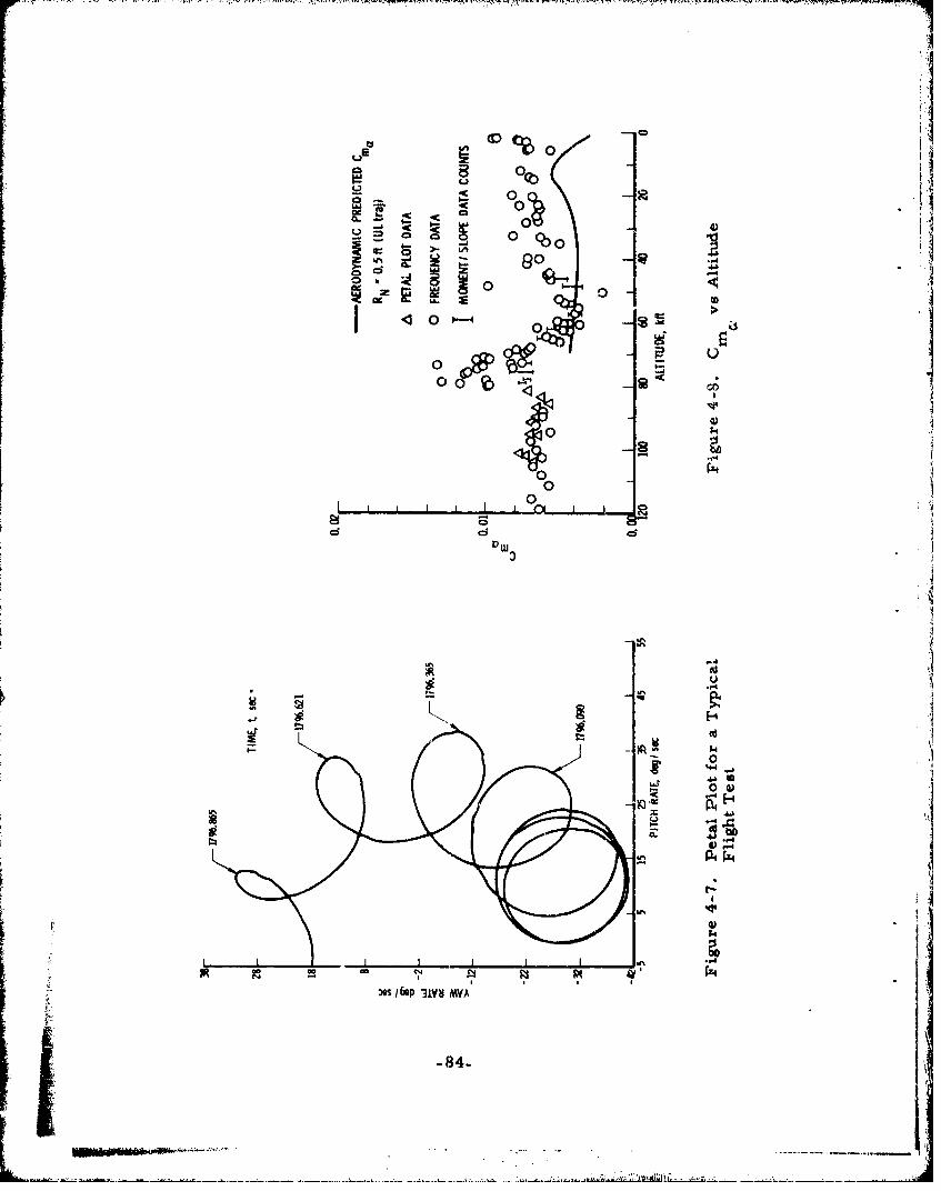
0- 0
O(Z)]
00 __0
04 ý
000%0 0I 0
i 0-
0000
0
d d d
1 ,w4
411
('33
00 Go 0 oo
M C-P MYo M
-84-
A _:
@i--
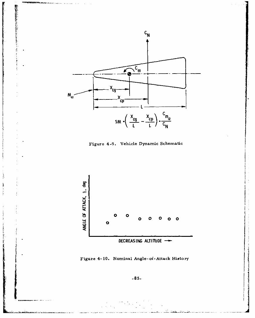
CN
NN
x 9- - c-- ------
Figure 4-9. Vehicle Dynamic Schematic
0 0 0 0 0 0 0
0 V
DECREASING ALTITUDE -- I ,Figure 4-10. Nominal Angle-of-Attack History
-85-
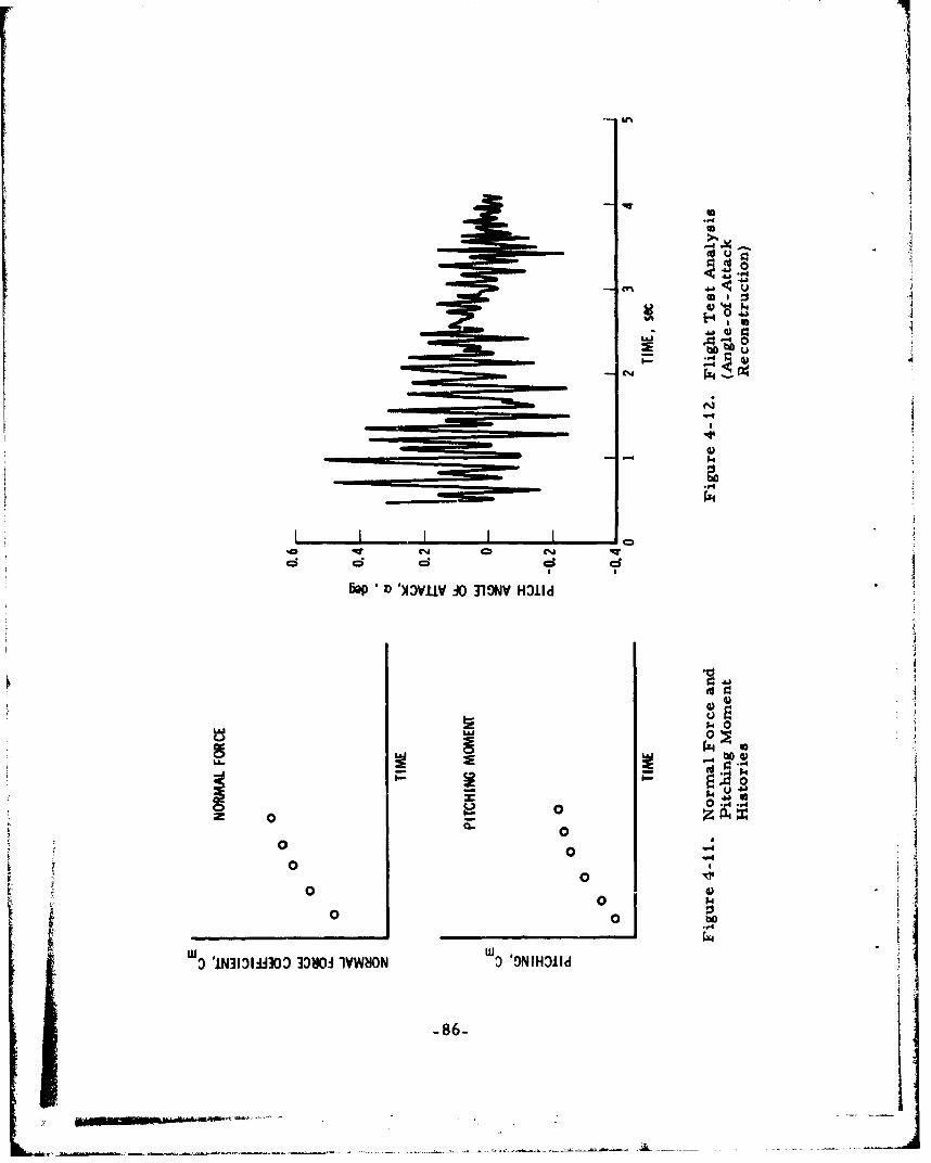
UNU
4,4'
P4
C; C;
'be 0 0
oc
z x
014)
-J 'IMI30 3080 IVSN3'9IO
-86-
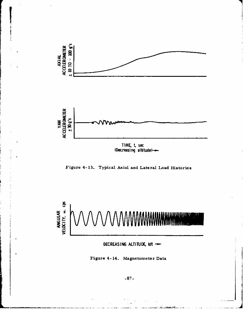
LU +
TIME, t, sec(Decreasing altitude)-a.-
Figure 4-13. Typical Axial and Lateral Load Histories
DECREASING ALTITUDE, kft -
Figure 4-14. Magnetometer Data
-877-
5. FLUID DYNAMIC MEASUREMENTS
5. I GENERAL
Fluid dynamic measurements consist of local flow field measure -
ments near the nosetip and on the frustum and base of an RV.
The basic fluid dynamic measurements consist of:
a. Heat transfer rate
b. Pressure (steady state)
C. Acoustic environment (fluctuating pressures)
d. Boundary layer transition (inferred from above)
The purpose of the measurements is essentially the same for the
previously discussed technologies; i.e.,* obtain in-flight measurements to
determine performance parameters to verify RV prediction, modeling, and
design techniques.
Since the measurement of interest is the local flow field at the
surface of the vehicle, it is important that the sensor not disturb the flow
field. The ideal sensor is one that would require no penetration of the sur-
face of the heatahield. Attempts to correlate subsurface temperature
measurements with surface and boundary layer phenomena have shown them
to have too great a time lag for useful data, and heat transfer measurements
require penetration of the heatahield. Fluctuating pressure measurements
can be made with either ported or nonported gages, as discussed later.
Ground tests and flight results show that holes less than -0. 050-in, diameter
do not affect transition, and ported gages can stay within this limitation.
Although the thermal gages fill the holes in which they are installed, they
do present a discontinuity at the surface. The gage and its installation must
be designed to minimize the disturbance. Flight results indicate that the
flow field is not disturbed sufficiently to trip boundary layer transition.
-89-
.1
5.2 HEAT TRANSFER MEASUREMENTS
Heat transfer measurements are made with either slug (integrating)
calorimeters or heating rate (differential) calorimeters. Photographs of
the differential-type sensors are shown in Figures 5-i and 5-2. The basic
purpose of these measurements is to obtain the change in heating rate as-
sociated with the onset of boundary layer transition from laminar to turbu-
lent flow. Both slug and rate calorimeters are mounted flush with the sur-
face of the heatshield. Slug calorimeters ccnsist simply of a copper mass
with a thermocouple to measure its temperature rise (AT). Neglecting
losses, the rise in temperature is proportional to the integrated heat input,
and a change in the rate of heat input is detected by a change in the rate of
rise.
Two types of rate calorimeters are in . tneral use. The first is a
Gardon type, manufactured by Hycal Engineering as their asymptotic
calorimeter. As shown in the cross section of Figure 5-3, the Hycal calo-
rimeters consist basically of a thin metallic foil of constantan, bonded on
the edges of a cavity in a heat sink of copper. A fine copper wire is bonded
metallurgically to the center of the foil. Heat flows into the surface of the
foil and then radially into the heat sink. The radial heat flow establishes a
radial temperature gradient, which is measured by the difierential copper-
constantan-copper thermocouple. It can be shown that q -AT -AV, so that
the output voltage varies with the rate of heat flow rate (q). A typical in-
stallation is shown in Figure 5-4.
The second type of rate calorimeter is the AT gage. As shown in
the cross section of Figure 5-5, heat flowing into the outer surface of the
gage establishes an axial heat flow with a resultant axial temperature
gradient. Two constantan wires, spaced axially, generate a voltage pro-
portional to the axial heat flow. Again, it can be shown that q/A - KAT -" AV,
so that, as with the Gardon gage, the out iut voltage varies with the heat
flow rate (q/A). For information, Figur,- ,-6 shows a photograph of the
internal portion of an RV with rate calorimeters installed.
-9')-
Several flight measurements have been made in which the two types
of rate calorimeters were flown "side by side' to compare performance.
K The flight results indicated that the two sensors tracked each other. respond-ing to changes in heat input due to variations in vehicle motion, and detected
the onset of boundary layer transition. Analog traces of typical flight data
for both sensors are shown on Figure S-7. The two sensors were at the
same body station and within 10* of each other. Figure 5-8 shows the pro-
gression of transition from aft to forward on a typical flight using the AT
sensor. Subsequent flights have further demonstrated that the progression
is from aft to forward, that the rate of progression varies, and that it can
be asymmetric.
5.3 STEADY STATE PRESSURE MEASUREMENTS
Steady state pressure measurements have been discussed previously
in the aerodynamics section. It was shown that local in-flight pressure
measurements (steady state) with a pressure port through the heatahield
connected to sensors within the RV were utilized to verify forebody and
base flow field prediction techniques. These flight data could be integratedto obtain the forebody and base drag components of total drag as discussed
in subsection 4.2.
In addition, base pressure measurements could also be utilized to
determine onset of boundary layer tranisition at the aft end of the frustum.
The above steady state pressure measurements can be made with relatively
low-frequency response pressure sensors (rise time < 30 msec) and sampling
rates as low as 10 to 20 samples/sec.f
5.4 ACOUSTIC MEASUREMENTS
Acoustic measurements are made for two basic purposes. First,
to determine acoustic overall sound pressure level (OASPL) due to fluctuating/
pressure, which emanates from the boundary layer during transitional and
turbulent flow, for structural analyses. Second. acoustic measurements
are an excellent indicator of onset of boundary layer transition, transition
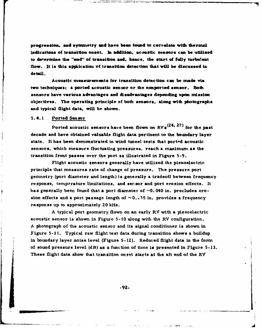
progression. and syamuetry and have been found to correlate with therma
indications of transition onset. In addition, acoustic sensors can be utilised
to determine the "end" of transition and, hence, the start of fully turbulent
flow. It is this appkication ef transition detection that will be discussed ir
detail.
Acoustic measurements for transition detection can be made via
two techniques: a ported acoustic sensor or the nonported sensor. Both
sensors have various advantages and disadvantages depending upon mission
objectives. The operating principle of both sensors, along with photographs
and typical flight data, will be. shown.
5.4.1 Ported Sensor
Ported acoustic sensors have been flown on RVs{2 4 ' 27) for the past
decade and have obtained valuable flight data pertinent to the boundary layer
state. It has been demonstrated in wind tunnel tests that ported acoustic
sensors, which measure fluctuating pressures, reach a maximum as the
transition front passes over the port as illustrated in Figure 5-9.
Flight acoustic sensors generally have utilized the piezoelectric
principle that measures rate of change of pressure. The pressure port
geometry (port diameter and length) is generally a tradeoff between frequency
response, temperature linmitations, and sensor and port erosion effects. It
has generally been found that a port diameter of -0. 040 in. precludes ero-
sion effects and a port passage length of "-0..5 in. provides a frequency
response up to approximately 20 kHz.
A typical port geometry flown on an early RV with a piezoelectric
acoustic sensor is shown in Figure 5-10 along with the RV configuration.
A photograph of the acoustic sensor and its signal conditioner is shown in
Figure 5-i1. Typical raw flight test data during transition shows a buildup
in boundary layer noise level (Figure 5-12). Reduced flight data in the form
of sound pressure level (dB) as a function of time is presented in Figure 5-13.
These flight data show that transition onset starts at the aft end of the RV
-92-
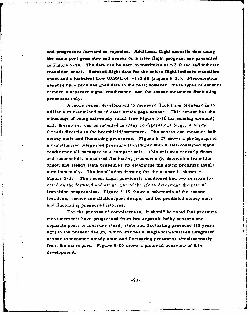
and progresses forward as expected. Additional flight acoustic data usingthe same port geometry and sensor on a later flight program are presented
in Figure 5-14M The data can be seen to maximize at - 2. 0 sec and indicate
transition onset. Reduced flight data for the entire flight indicate transition
onset and a turbulent flow OASPL of - 150 dB (Figure 5 -IS?. Piezoelectric
sensors have provided good data in the past; however, these types of sensors
require a separate signal conditioner, and the sensor measures'fluctuating
pressures only.
A more recent development to measure fluctuating pressure is to
utilize a miniaturized solid state strain gage sensor. This sensor has the
advantage of being extremely small (see Figure 5-16 for sensing element)
and, therefore, can be mounted in many configurations (e.g., a screw
thread) directly to the heatahield/ structure. The sensor can measure both
steady state and fluctuating pressures. Figure 5-17 shows a photograph of
a miniaturized integrated pressure transducer with a self-contained signal
conditioner all packaged in a compa:7t unit. This unit was recently flown
and successfully measured fluctuating pressures (to determine transition
onset) and steady state pressures (to determine the static pressure level)
simultaneously. The installation drawing for the sensor is shown in
Figure 5-18. The recent flight previously mentioned had two sensors lo-
cated on the forward and aft section of the RV to determine the rate of
transition progression. Figure 5-19 shows a schematic of the sensor
locations, sensor installation /port design, and the predicted steady state
and fluctuating pressure histories.
For the purpose of completeness, it should be noted that pressure
measurements have progressed from two separate bulky sensors and
separate ports to measure steady state and fluctuating pressure (10 years
ago) to the present design, which utilizes a single miniaturized integrated
sensor to measure steady state and fluctuating pressures simultaneouslyfrom the same port. Figure 5-20 shows a pictorial overview of this
development.
-93-
Typical fluctuating pressure data from the ported acoustic sensors
are presented in Figure 5-Z for the aft and forward sensors. The data
show the expected trend of transition initiation at the aft end and progressing
forward. The aft sensor indicates transition onset at t - 0.5 sec. while the
forward sensor indicates transition at t - 3.5 sec. This time span is con-
sistent with thermal indications. As stated previously, the solid state
strain gage sensors can measure steady state and fluctuating pressutres
simultaneously and are illustrated in Figure 5-22.
5.4.2 Nonported Sensor
The nonported acoustic gage is a recent development called the33
Boundary Layer Acoustic Monitor (BLAM) gage. This gage has been
flight-tested with rate calorimeters for comparison. As shown in
Figure 5-23, the sensing element is mounted on the inside of the heatshield
and senses the acoustic noise in the flow field by the stress waves trans-
mitted through the heatshield. It achieves the ideal sensor objective of
requiring no holes in the heatshields. By good design and choice of
frequency, the sensor is made highly directional and has a narrow-band
frequency response, with typical results of Figure 5-23. A typical vehicle
installation is shown in Figure 5-24; an internal RV, in Figure 5-25.
Due to the wide range of sound pressure levels, the BLAM signal
conditioner converted the input signal to a log output sig al. As shown in
Figure 5-26, the resultant output gave clear indications of the presence of
noise bursts well before the rate calorimeters indicated thermal transition.
It should be noted on Figure 5-26 that the noise burst occurs out of phase
on the two sides of the vehicle. The noise on one side is not detected on
the opposite side, indicating clearly the direction sensitivity of the detectors.
Careful comparison of the observed peaks in the noise signal with vehicle
motion indicated a close correlation with angle-of-attack variations, even
though the maximum angle of attack at this time was less than 0.2 deg.
Due to the compression of the log scale, acoustic transition is not
easily detectable on Figure 5-26. The same data is showti on Figure 5-27
-94-
or, a linear output scale. Acoustic transition is indicated clearly, and thesensors indicate that the transition occurs simultaneously on both aides.
The thermal transition detectors on this vehicle, however, consistentlyIshowed an asymmetric transition. Incidentally, the thermal sensors showedthe same correlation with vehicle motion shown by the acoustic sensors.
A comparison of the BLAM output for a typical flight shows it does sense
transition progression from the aft to forward station as expected(Figure 5-28).j
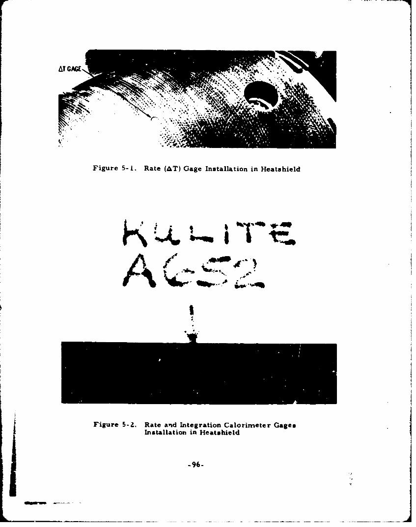
Figure 5- L Rate (AT) Gage Installation in Heatuhield
hft
Figure 5-2. Rate anid Integration Calorimeter GagesI Installation in Heatshield
-96-
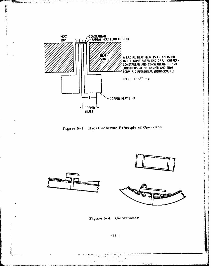
HEAT CONSTANTANINPUT ,RADIAL HEAT FLOW TO SINK 'I
/TA RADIAL HEAT FLOW IS ESTABLISHED
"IN THE CONSTANTAN END CAP. COPPER-TCONSTANTAN AND CONS'ANTAN-COPFER•' JUNCTIONS AT THE CENTER AND ENIUS
FORM A DIFFERENTIAL THERMOCOUPLE
JNTIONS EAT T-q~.NE NDED
"E-COPPER HEAT SILK
COPPER-
Figure ;-3. Hycal Detector Principle of 0peration
Figure 5-4. Calorimeter
-97-
.."... ... ..... " * 1'"' ., 2 " -
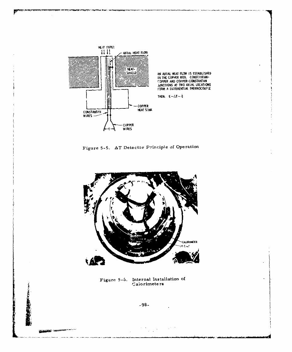
HEAT INPU,
SU AXIAL HEAT FLOW
j /
S H L AN AXIAL HEAT FLOW IS ESTABLISHED<7 7/IN THE COPPER ROD. CONSTA.NTAN-
rOPPER AND COPPER-CONSTANTAN; IJdNCTIONS AT TWO AXIAL LOCATIONS7 1) FORM A DiFFERENTIAL, THERMOCOUFiE
THEN: E-AT-•q
L, -COPPER
CONSTANTAN HEAT SINK
WIRES -
COPPERE WIRES
Figure 5-5. AT Detector Principle of Operation
•CAL001IfRR
Figure 5-/. Lnternal Installation ofCalorimete rs
!. -g_-8 -
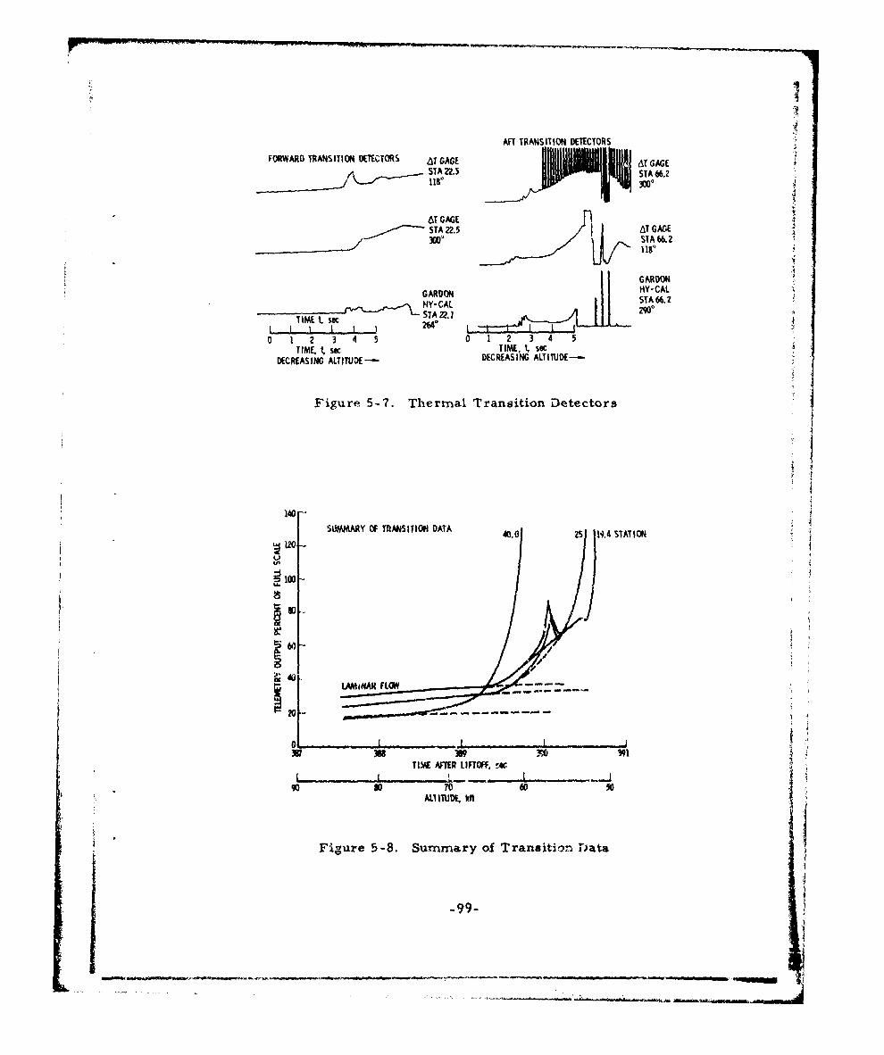
'I
AFT TRANSITION DETECTORS
FORWARD TRANSITION DETECTORS AT GAGE At GGE.
5TA 22.5 STA 66.2
AT GAGE
STA22.5 AT GAGE300- STA 66. 2
1180
GARDON
GARDON NY-CALNY-CAL TA66.2
TIME t sec STA 22.126,4*0 t
0 1 2 3 4 5 0 1 2 3 4 5TIME. t, sa TIME, t, sec
DECREASING ALTITUDE- DECREASING ALTITUDE-
Figure 5-7. Thermal Transition Detectors
1401
SUMMARY OF TRANSITION DATA 0.0 25 19,4 STATION
60
AiMRFLOW •
011
TIMIE AFTER LIFTOFF, . : ,w•
960so0 00
AL ITUE f
Figure 5-8. Summa ry of TransitTon Data
-99- •:
• .I
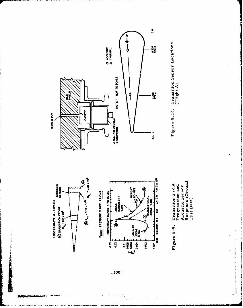
Ii 0LUU
.41
ci 0 0
U) M4 -
00
-j-
-Lob
ac K
LU LA
0 -toao- ~
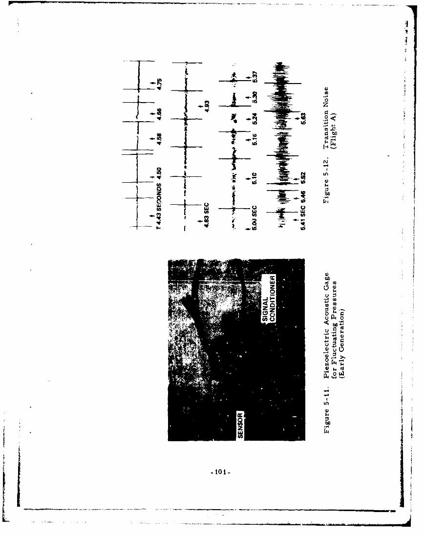
4-) 4ý
'd4~ - .,q i
F~4
$4
-~ -4
1 $180 14 g- sIee C., -
4. 4
4bO
U)
4J
-lot-
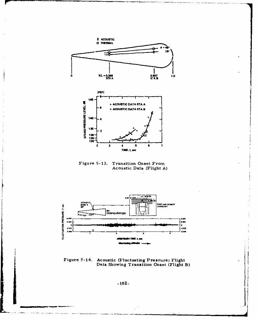
9 ACOUSTIC0 THERMAL
0 X/L 0.368 0.607 1.0STA A S-A 8
IPSF)
146a ACOUSTIC DATA STA A
6 a ACOUSTIC DATA STAB
1CUSI 0--440SPIO
0013522
4z
Datar Sh1.owasiing Trnsitio Fom~t(lgtB
Acu102- ta(lihtA
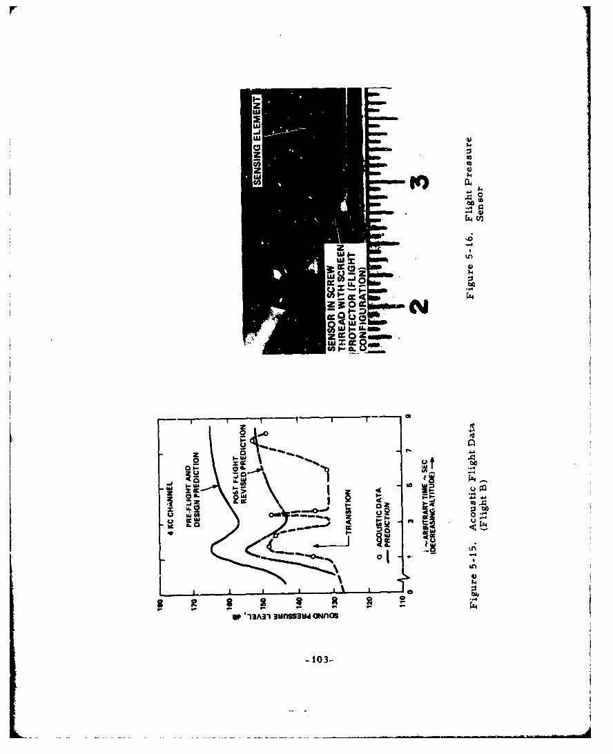
prz
$4U
uIl
134
0$-0
LU k
UjU)
0 03
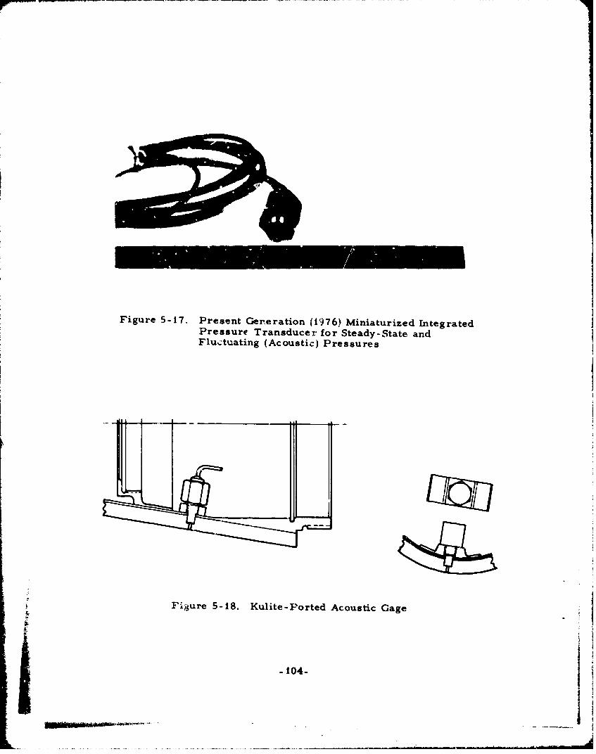
Figure 5-17. Present Generation (1976) Miniaturized IntegratedPressure Transducer for Steady-State andFluctuating (Acoustic) Pressures
Figure 5-18. Kulite-Ported Acoustic Gage
-104-
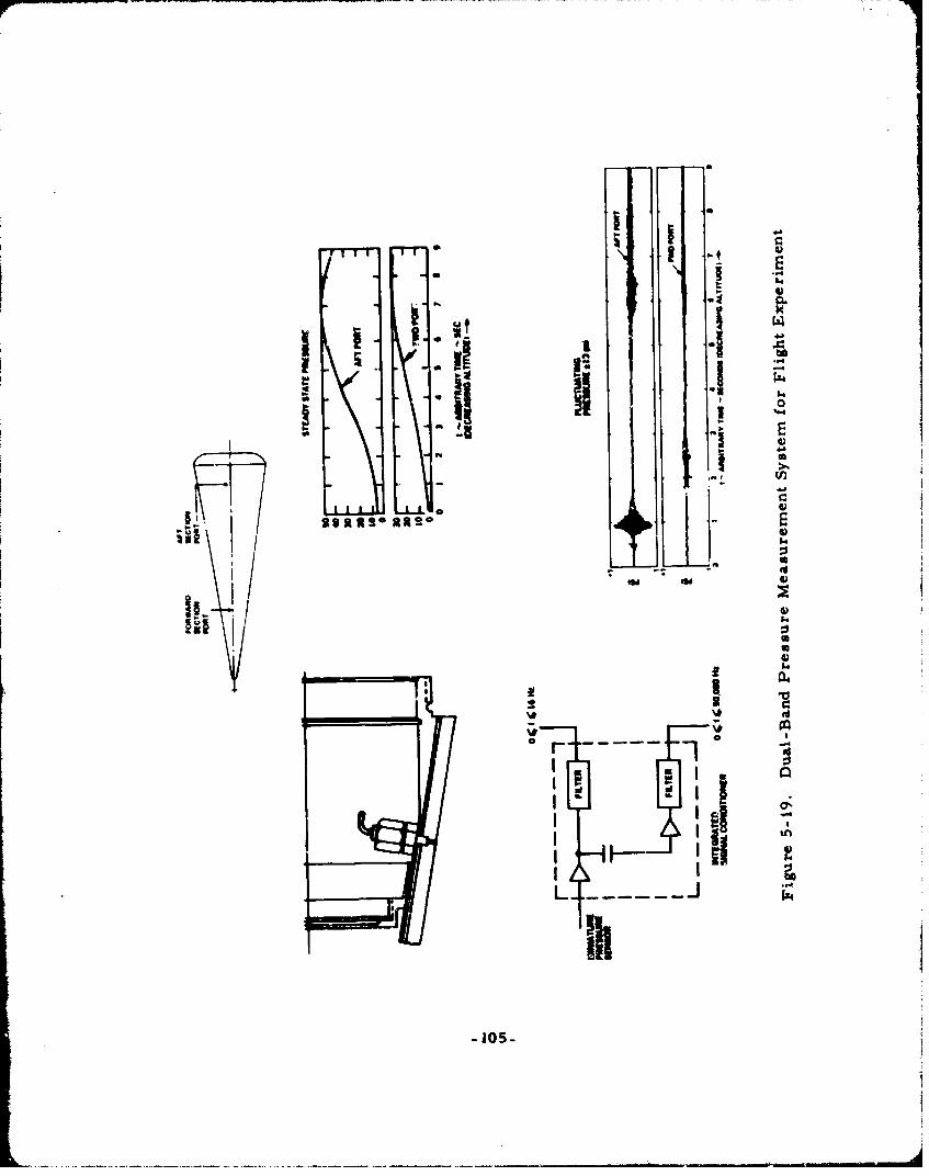
r-w --
A ag
4%4
Sul 14X1 I '
24.
V.N& ZA
-a
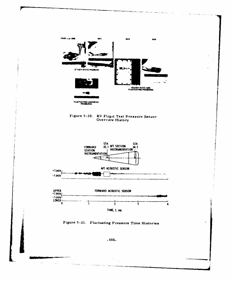
U-?,
tWY STATE 1Pý180ftE
DTIOY STATE AN -FLUCTUATWH PM880IS
FLUCTUATING IArLTOUIC)PRISSUNS
Figure 5-ZO. RV FLig-it Test Pressure SenrorOverview History
STA STA
FORWARD 22.1 R S •ION 66.2STATION INSTRUMENTAT1ONINSTRUMIENTATION
AFT ACOUSTIC SENSOR
-1 psia" --- - "
UPPER FORWARD ACOUSTIC SENSOR+I psia•.•- :
LOWER,• .. . . -•. .0 1 2 3 4
TIME, t sK
Figure 5-21. Fluctuating Pressure Time Histories
-106-
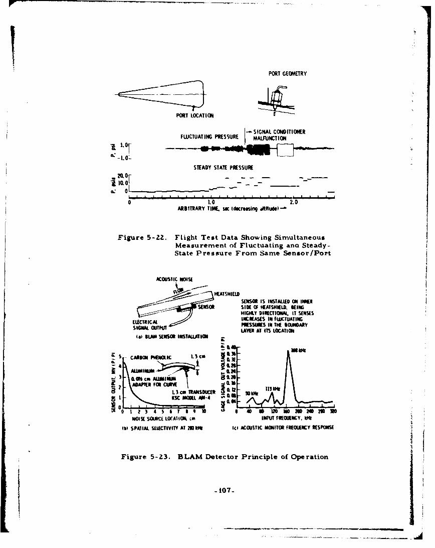
PORT GEOMETRY
PORT LOCATION
SIGNAL CONDITIONERFLUCTUATING PRESSURE MALFUNCT ION
STEADY STATE PRESSURE
20. -10o0 - -_ _--
0
o L0 0.0ARBITRARY TIMW sc (decrisinq iftfudl)
Figure 5-22. Flight Test Data Showing SimultaneousMeasurement of Fluctuating ana Steady-State Pressure From Same Sensor/Port
ACOUSTIC NOISE
j~HLATHIELOSENSOR IS INSTALLED ON INNER
SENSORSIDE OF HEATSNIELO. KEINGHIGHLY DIRECTION1l. IT SENSES
ELECTRICAL PESSUES IN TiE IOUNDARYSIGNAL OU.'IIT LAVER AT ITS LOCATION
Is) KAM SENSORIALIAN -i
_____CAR _ON PHENOLIIC L 3 cm v &II
•!6 -4
- M 1 116
0 23 5 7 9 1 6U U00 ED UO0 ! 7 a lqI 40 10 12 IO me M MI INo
NOISE SOURCf LO(A1ION, 4m INPUT FREQUIENCY. k,
ISII $PATIAL SELECTIVITY AT 2 ftt Io ACOUSTIC MONITOR FRECUENCY RESPONSE
Figure 5-Z3. BLAM Detector Principle of Operation
-107--L- - - .
-iln
Figure 5-24 Transition Acoustic
NOPORTEDACOUSTIC
S• PORTED GAGE GG
ACOUSTIC ,''
SENSOR
Figure 5-Z5. Internal RV
- 108-
3-3
228
>. 4 2--
z
•3
2, 2THERMAL TRANS ITION
S~118*
012 3 4 5
REFERENCE TIME, sec
Figure 5-26. Kaman (BLAM) TransducerOutput
70-
128' MERIDIAN
MERIDIAN40-20
TIHERMAL TRANSITION
0 1 2 3 4 5REFERENCE TIME, seC
Figure 5-27. Kaman Detector
j -109-
- M, IMP
KAMAN DETECTOR~..- STA 22. 1
87 0
FORWARD SENSOR
DECREASING ALTITUDE, kit -
KAMANSTA 66.21280 MERIDIANAFT SENSOR
-BAASE PRESSURE0-0.5 psiaFORWARD SENSOR
1111I
- DECREASING ALTITUDE, kit
Figure 5-Z8. Nonported Acoustic Sensor
6. OFF-BOARD INSTRUMENTATION
The KREMS (Kiernan Reentry Meavsurement Site) is an instrument
system composed principally of three radars and a variety of optical instru-34
mentation and computer subsystems. The PRESS (Pacific Range Electro-
magnetic Signature Studies) computer is used to transfer steering informa-
tion from one instrumentation component to another or to provide initial
steering information to any single radar or optical component of the system.
The interaction between components is shown schematically in Figure 6-i.
In addition to these major components, there exist a variety of lesser
instrumentation at various points throughout the Kwajalein Missile Range
(KMR). These are located on the map of the range (Figure 6-2) and will be
discussed later.
The major radars are C-band, L- and S-band, and V or UHF sys-
tems. Probably the C- and L/S-band systems are the most important to
SAMSO Programs since the longer wavelength radar is concerned primarily
with long-range reentry vehicle detection; however, the short wavelength
systems provide better spatial resolution, thereby giving better information
relative to reentry vehicle performance and accuracy, which is the eventual
r zzf of the success or failure of a SAMSO program. Thus, the C-band
system (ALCOR) and the S/L-band system (TRADEX) are usually mandatory
pieces of instrumentation on SAMSO flights. The 68-ft space frame radome
of the ARPA-Lincoln C-Band Observable Radar (ALCOR) is shown in
Figure 6-3 with the TRADEX antenna in the background. ALCOR was
designed to study very wide bandwidth observables associated with targets
reentering the atmosphere at high velocities. It his been in operation since
January 1970.
ALCOR is a wideband C-Band radar with the exceptional rangeresolution of 0. 5 m. This resolution is achieved by transmitting and process-
ing the returns from a 512-MHz bandwidth linear chirp signal. Since the
-ill-
_ . .. . ¿• 4 ' : ' ' , +, . . .. . , . . . . .I S-, W
bandwidth ;.s so wide, real-time digital. recording would normally be
difficult. To alleviate this problem, the ALCOR receiver uses a time-
bandwidth exchange technique that reduces the real-time bandwidth without
loss of the range resolution correspondirng to the original bandwidth. Using
this method, data can be collected and recorded over a range interval of
90 rn on each PRI (Pulse Repetition Interval).
A narrowband waveform covering a range window of 2. 5 km is
available for simultaneous use with the wideband tracker. The larger range
window is useful for acquiring targets. ALCOR also has the ability to
acquire and track the beacons that are flown on the major components of a
target complex. Up to four different be:acon codes can be accommodated
by the systerm, giving ALCOR the capability to sequentially beacon track
more than one object in a reentry complex. The characterist-ics of ALCOR
are given in Table 6-1. The sensitivity of the radar is shown in Figure 6-4.
The TRADEX (Target Resolution and Discrimination Experiments)
dual-frequency, high-power instrument radar can track in S- or L-band
with F'multaneous operation at the other frequency. A high-speed digital
computer is the core of the radar system. Using real-Lime processing, the
computer provides operational control of the radar by selection of the radar
parameters, is an integral part of the range and angle tracking loops, drives
displays, and controls the recording subsystem and processing.
The system operates coherently with a wide variety of wide band-
width linear-frequency modulated pulses and pulse bursts available for
transmission on both bands. At L-band, these waveforms are generated by
an active exciter for the chirp waveform and tapped delay lines for the burst
waveform. At S-band, the chirp and burst waveforms are generated pas-
sively by expansion networks. There are 13 receiver channels used to
accommodate the various combinations of S/L-band transmitted chirp and
burst waveforms.
The L/S-band digital-data recordings systems contain logarithmic
amplifiers and phase detectors whose outputs are sampled by high-speed
i i -liz-
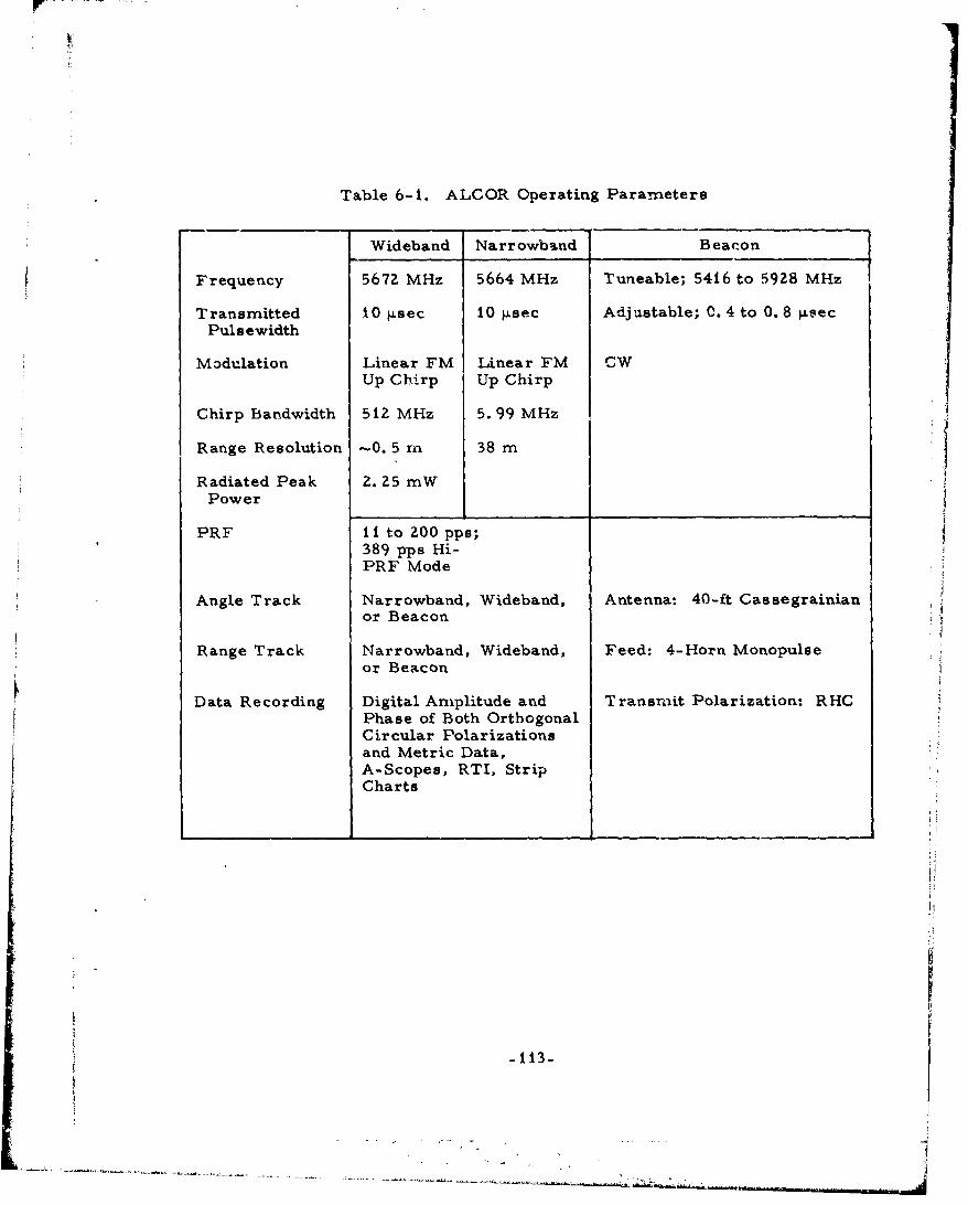
Table 6-i. ALCOR Operating Parameters
Wideband Narrowband Beacon
Frequency 5672 MHz 5664 MHz Tuneable; 5416 to 5928 MHz
Transmitted 10 tsec 10 psec Adjustable; 0. 4 to 0.8 4secPuls ewidth
Modulation Linear FM Linear FM CW
Up Chirp Up Chirp
Chirp Bandwidth 512 MHz 5. 99 MHz
Range Resolution -0.5 rn 38 m
Radiated Peak 2. 25 mWPower
PRF II to 200 pps;389 pps Hi-PRF Mode
Angle Track Narrowband, Wideband, Antenna: 40-ft Cassegrainianor Beacon
Range Track Narrowband, Wideband, Feed: 4-Horn Monopulseor Beacon
Data Recording Digital Amplitude and Transmit Polarization: RHCPhase of Both OrthogonalCircular Polarizationsand Metric Data,A-Scopes, RTI, StripCharts
I!
-113-
analog-to-digital converters. At L-band the highest sampling is 10 MHz;
at S-band it is 60 MHz. Phase and amplitude samples are accumulated,
stored, and subsequently recorded on tape with simultaneous metric, mode,
and status data. Pre-mission alignment and calibration of the radar is
accomplished by built-in test equipment under computer control. There
are test signals, continuous wave (CW) chirp pulses, and radio frequency
(RF) chirp pulses available for insertion at various points in the receiver
chain.
The characteristics of TRADEX are given in Table 6-2, and the
sensitivity of TRADEX is given in Figure 6-5.
In addition to RV radar cross section (RCS) and metric data,
ALCOR and TRADEX are used to gather environmental information. This
function is of major importance in both clear air and weather environments.
In weather-penetrating RV flights, these radars are used to measure the
water content on the trajectory. In clear air flights they are used (particu-
larly ALCOR) to ensure that a specified threshold water content is not
exceeded prior to launch in the reentry corridor. The sensitivity of these
radars relative to weather environments is shown in Figure 6-6.
The ARPA Long-Range Tracking and Instrumentation Radar
(ALTAIR) (Figure 6-7) became operational in early 1970; it is a highly
sensitive, dual-frequency radar that gathers coherent target return data
simultaneously at VHF and UHF. Good long-range performance and excel-
lent range resolution are obtained using both CW and linear frequency
modulation pulse compression.
In operation, a central object in a multitarget complex is selected
for computer-aided range and monopulse angle tracking at VHF (very high
frequency) or UHF (ultrahigh frequency). The ALTAIR Recording System,
with its separate computers, then acquires, range tracks, and records
data on the multiple targets that are illuminated by the VHF and UHF beams.
* Digital data are recorded simultaneously on as many as 14 targets with a
total capacity of up to 56 X 106 bps.
-114-
""1"il • .. .-..... . .
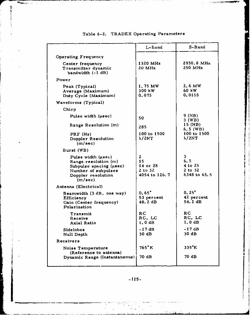
Table 6-2. TRADEX Operating Parameters
L-Band S-Band
Operating Frequency
Center frequency 1320 MHz 2950.8 MHzTransmitter dynamic 20 MHz 250 MHz
bandwidth (-I dB)
Power
Peak (Typical) 1. 75 MW 2. 6 MWAverage (Maximum) 300 kW 60 kWDuty Cycle (Maximum) 0. 075 0.0165
Waveforms (Typical)
Chirp
Pulse width ("sec) 50 9 (NB)3 (WB)
Range Resolution (m) 285 15 (NB)
PRF (Hz) 100 to 1500 100 to 1500Doppler Resolution X/2NT X/2NT
(m/sec)
Burst (WB)
Pulse width (g.sec) 2 3Range resolution (m) 15 6.5Subpulse spacing (ýLsec) 14 or 28 4 to 25Number of subpulses 2 to 32 2 to 32Doppler resolution 4054 to 126. 7 6348 to 63.5
(m/sec)
Antenna (Electrical)
Beamwidth (3 dB, one way) 0.650 0.250Efficiency 53 percent 42 percentGain (Center frequency) 48. 2 dB 54. 2 dBPolarization
Transmit RC RCReceive RC, LC RC, LCAxial Ratio 1. 0 dB 1. 0 dB
Sidelobes -17 dB -17 dB
Null Depth 30 dB 30 dB
Receivers
Noise Temperature 765" K 3350K(Reference to antenna)
Dynamic Range (Instantaneous) 70 dB 70 dB
-I15-
A series of modifications were completed in the spring of 1973
that gave the ALTAIR system an angle tracking and recording capability at
UHF in addition to the existing VHF capability. Its operating parameters
are given in Table 6-3.
The Army Optical Station at KREMS (Kierriian Reentry Mearure-
ments Site) provides a test-bed for two passive infrared scanning
radiometeis (WAS and GBM) and an active infrared laser radar (LITE).
The passive sensors will be operated to develop a data base on reentry
bodies for the purpose oi optical adjunct performance evaluation. The laser
radar will be operated to develop a data base of laser cross sections of the
various reentry bodies and the particulate wake.
In addition to gathering this cross-sectional data, the LITE sys-
tem (Table 6-4) will be used as a practical demonstration of the techniques
involved in using a laser radar in the KREMS environment; for example,
experience will be gained from the reentry acquisition problem, system
calibration, and handover from the laser to a microwave radar.
The wide-angle sensor (WAS) is a ground-based infrared system
operating in the LWIR (long wavelength infrared) region. It has a wide field
of view (WFOV), 60 in azimuth. The detector array consists of two vertical
columns of 50 detectors offset in azimuth and interleaved in elevation.
Each detector covers a field of I X i mrad. The scan frequency is variable
in the following steps: 0. 2, 0. 3, 0. 5, 0.8, 1. 25, and 2. 0 Hz. The operator
is provided with a C-scope display of the detector outputs.
Data are recorded on ar% analog tape recorder and on digital tape
with the NOVA Control and Recording System (NCRS). Boresighted LLTV-
TV and 35-mm cameras provide additional supporting data.
The GBM-2 system provides high-resolution radiometric data on
selected targets of interest. It is computer directed and when completely
integrated into the AOS (acquisition of signal) will have backup acquisition
and track capability. GBM-2 operated in both LWIR and SWIR (short
wavelengeh infrared). It has an FOV 5 mrad in azimuth and 2. 5 mrad in
-116-
~-----. ~ ~_'
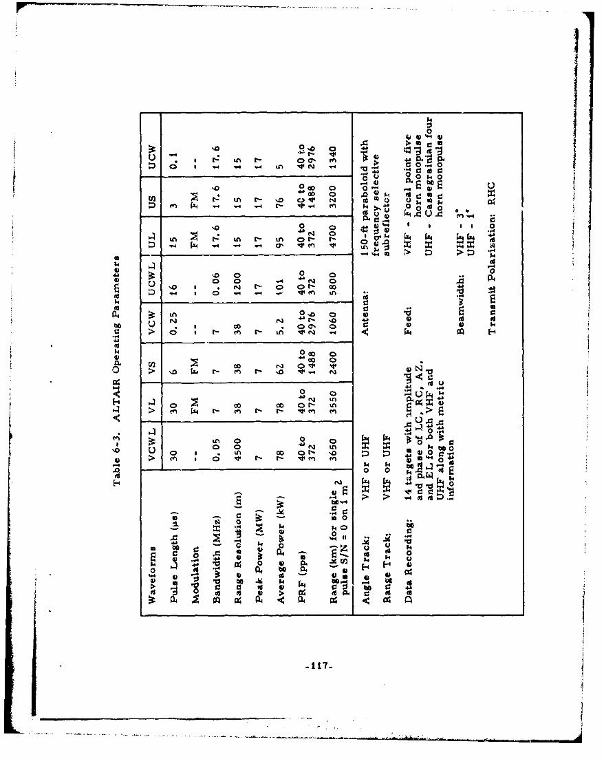
LIi. - v
0. Lj > U)-
0 0 o~ NJ4o4
~~~c 0 10 a6L 6'N -a .
to 0
U) tn r -q -c) ;
-4 P4 -4 -4 .-. L L
0 0
cU '. 00 U-4 4 LA t!~
H4L 0,0 0'Ii OD~ o
LA000 0O 00 ItN vA v
'.0 U 0 S * LA0 O4 '0 W S o0.C) ~ 00 00- 01(n L H
(UH N.1 4WO
.0.en *n H 04
Cý c U) 00I U'
00 0~ 0~to 'dPU)t
Iw vU4.
All z
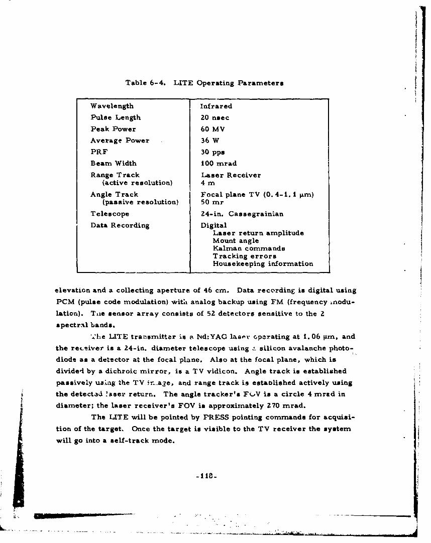
Table 6-4. LITE Operating Parameters
Wavelength Inf rared
Pulse Length 20 nsec
Peak Power 60 MV
Average Power 36 W
PRF 30 pps
Beam Width i00 mrad
Range Track Laser Receiver(active resolution) 4 m
Angle Track Focal plane TV (0.4-1. 1 Rm)(passive resolution) 50 mr
Telescope 24-in. Cassegrainian
Data Recording DigitalLaser return amplitudeMount angleKalman commandsTracking errorsHousekeeping information
elevation and a collecting aperture of 46 cm. Data recording is digital using
PCM (pulse code modulation) wit'i analog backup using FM (frequency inodu-
lation). Tae sensor array consists of 52 detectors sensitive to the 2
spectral bands.
'..he LITE trarnsmitter is a Nd:YAG lastar cparating at 1. 06 inm, and
the receiver is a 24-in. diameter telescope using ý silicon avalanche photo-
diode as a detector at the focal plane. Also at the focal plane, which is
divided by a dichroic mirror, is a TV vidicon. Angle track is established
passively uaslng -he TV ir.-a~e, and range track is estaolished actively using
the detected !aser return. The angle tracker's FOV is a circle 4 mrad in
diameter; the laser receiver's FOV is approximately 270 mrad.
The LITE will be pointed by PRESS pointing commands for acquisi-
tion of the target. Once the target is visible to the TV receiver the system
will go into a self-track mode.
j -lI1-
""" 1-~-

Data are recorded digitally under control of the real-time program
that resides in the LtTE's MODCOMP computer. The image produced by
the tracking TV is rrcorded on an IVC video tape recordur. A boresighted
surveillance TV provides additional supporting data. This TV is fitted with
a zoom lens that is continuously adjustable from 3" to 30' F'OV.
A possible future ABRES use for the TATE sensor is in a direct
measurement of a clear air environment; i. e., to ascertain if less than
specified threshold of water content eists at altitude in the reentry corridor
before launch or after splauhdown. The sensitivity of LITE is shown in
Figure 6-8. Note that it is about two orders of magnitude better than
ALCOR.
A rather unusual piece of instrumentation available at Kwajalein is
the ABRES weather aircraft (Figure 6-9). The Lear jet, with an operating
ceiling of 45 kft, is used to "calibrate" ALCOR or TRADEX to the particular
type of environment that exists at altitudes in the reentry corridor. This
is accomplished by using the MPS-36 at Kwajalein Missile Range (KMR) to
track the Lear aircraft during a "sampling" run. This tracking information
is processed in the Kwajalein CDC-6600 computer producing steering infor-
mation required to aim ALCOR or TRADEX to a point directly in front of
the Lear. Consequently, the radar measures the reflectivity in a range gate in
front of the sampling aircraft, which is in turn measuring the water content of
the environment. Thus, the measured reflectivity is "calibrated" to the
cloud water content, and radar measurements at spatial points not sampled
by the aircraft can be evaluated in terms of water content.
The instruments aboard the Lear are primarily "particle counter"
types that determine one or two dimensions of the ice crystal or water
droplet and catalog them in size ranges from 2 to 5000 gLm. For such a
large size range. thfsb different instruments are required. This informa-
tion i- periodically fed into an onboard computer that calculates mass from
the measured particle distributions. This mass information and the dis-
tributions are telemetered to the ground. In addition to the size measure-
ment, various "housekeeping" information is available; i.a., position,
-119-
-----------------------------
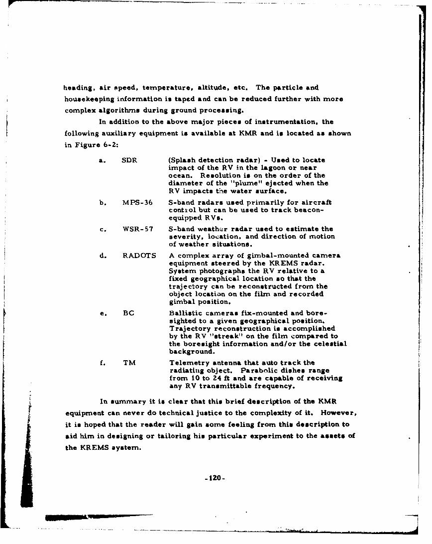
heading, air o'peed, temperature, altitude, etc. The particle and
housekeeping information is taped and can be reduced further with more
complex algorithms during ground processing.
In addition to the above major pieces of instrumentation, the
following auxiliary equipment is available at KMR and is located as shown
in Figure 6-2:
a. SDR (Splash detection radar) - Used to locateimpact of the RV in the lagoon or nearocean. Resolution is on the order of thediameter of the "plume" ejected when theRV impacts the water surface.
b. MPS-36 S-band radars used primarily for aircraftcontrol but can be used to track beacon-equipped RVs.
C. WSR-57 S-band weather radar used to estimate theseverity, location, and direction of motionof weather situations.
d. RADOTS A complex array of gimbal-mounted cameraequipment steered by the KREMS radar.System photographs the RV relative to afixed geographical location so that thetrajectory can be reconstructed from theobject location on the film and recordedgimbal position.
e. BC Ballistic cameras fix-mounted and bore-sighted to a given geographical position.Trajectory reconstruction is accomplishedby the RV "streak" on the film compared tothe boresight information and/or the celestialbackground.
f. TM Telemetry antenna that auto track theradiatitig object. Parabolic dishes rangefrom 10 to 24 ft and are capable of receivingany RV transmittable frequency.
In summary it is clear that this brief description of the KMR
j equipment can never do technical justice to the complexity of it. However,
it is hoped that the reader will gain some feeling from this description to
aid him in designing or tailoring his particular experiment to the assets of
the KREMS system.
-120-
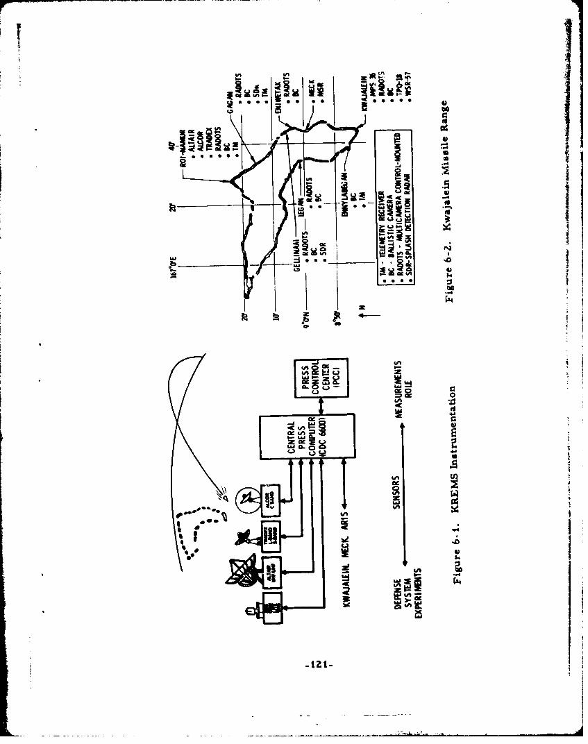
V I 4 A1
Lai
I -C
1'1414A1
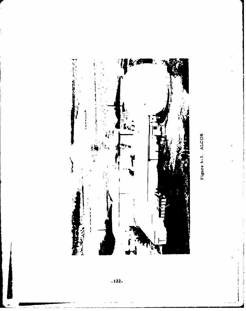
I,
I *�
m1 j.'.j. - ?i:yE'
'a�
$ � A 41:
4 -
-'I, I l.a
h.1
I ti-�
$1 V I.I III I
) I4 I
*1�
- 122-
iiI
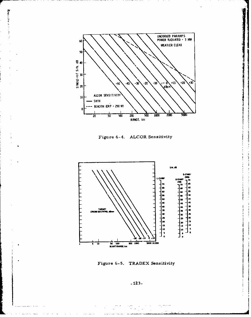
•! -• ••UNCOLED PARAMPS
60 POWER RADIATED 3 MOM
WATHlER CLEAR
40 -
t \
.-7-- BEACON (EPP- 250 W)
2 50LO 0 500 1000 2000
RANGE kmJ
Figure 6-4. ALCOR Sensitivity •"
46 so
InII
bsm 50
so., S o 4S
45 4S 40
CRM ~ ~ ~ ANE kmTM ~w3 53
-30 30 25
- 6 2S 20 1
SIs 10
"--0 0620 -lo0 +10
to0 90 100 9SO I000 §000 I0.000SLANT *ANN, km
Figure 6-5. TRADEX Sensitivity
_123-
45 45 i
. . . ... . ... .. ... ..... .. . • . ... .. . .. .. . .. . . . ... . .. .. . ..... . . . ... ... ... . .. _. ... .. . •. . . .. ... . .. . . • . .40 , - - 40. . . , . ..
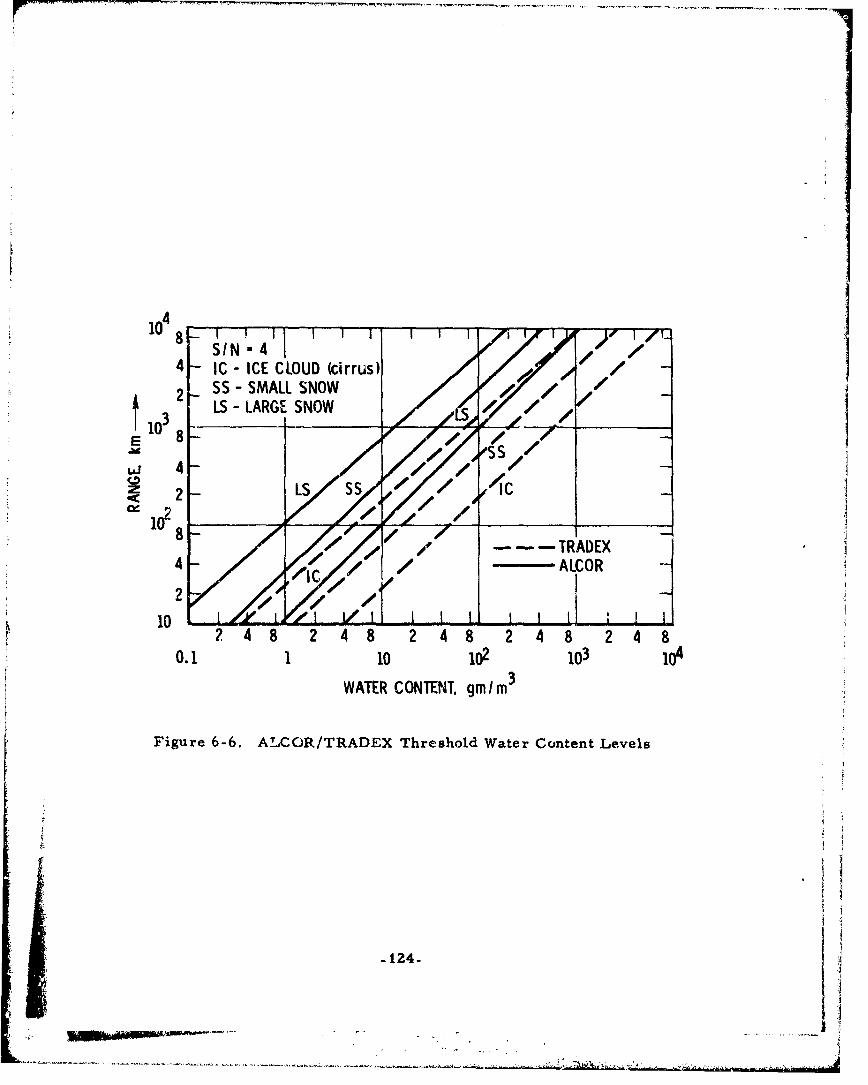
4- IC - ICE CLOUD (cirrus)2 SS - SMALL SNOW
LS - LARGE SNOW _______110 38 - 0 Z X- / "/-
108,0 1 e/ ---- TRADEX
10 24 8 2 48 2 48 2 48 24 80.1 1 10 iz2 io3 o
WATER CONTENT, gm rn3
Figure 6-6. ALCOR/TRADEX Threshold Water Content Levels
< 2- 124-
/ C2 . 0
VolIlb4
dvH
4J
CKC
caCh.
if
0 a'c00-4
- 0
'I: 43
43
cm as 00 tv go00
--- M '83MOd 03AOI333
~1~t26-
7. INSTRUMENTATION ASPECTS OF
FUTURE REENTRY TESTING
In planning the program for reentry system R&D for tfe next
decade, the primary objectives will continue to be in the areas of
defense penetration and of survival with accuracy in natural and hostile
environments. However, one can expect to see an increasing P-nphasis on
maneuvering RVs, as opposed to ballistic RVs, due to the pot.',tial deploy-
ment of high-performance interceptors and to the need for high accuracy.
Ballistic reentry technolcogy is rmaching a mature plateau Iin many areas due to recent activities and achievements. One critical area
remaining is reentry performance in adverse weather.
7.1 WEATHER EFFECTS ON REENTRY VEHICLE
PERFORMANCE
In recent years, our understanding of the phenomena that change
the performance of an RV when it flies through clouds of water, ice, or
snow particles has improved very rapidly. Basically, there are changes
induced in the surface roughness and nose shape that alter, usually increasing,
the drag force so that the vehicle falls short of its intended impact point.
It should be admitted at the outset that there is little hope
that these phenomena can be made the subject of precise predictions for
operational ballistic RVs. Our lack of knowledge of the precise meteorology
* that will exist when the vehicles arzive at the target e.rea will pr-ccude the
inclusion of an accurate bias in the targeting software. At best we can only
include a statistical correction of the same nature currently used for seasonal
winds and density. Meanwhile, we will attempt to design our vehicles to be
as insensitive to adverse weather effecits as possible.
An alternative approach is to add some form of aerodynanmic
control to the vehicle. The two ends of the spectrum are full three-axis
-i27-
control and single-axis drag modulation and some inertial instrumentation
with the objective of flying an inertial path independent of the ambient
weather. In this event, the weather problem reduces to enduring that the
vehicle has sufficient thermal protection to survive to impact.
For either approach in the R&D flight test phase, we need
to correlate vehicle shape and performance changes with the actual weather
environment on the reentry path. This latter item is difficult to achieve with
the required accuracy. Currently, the technique consists of flying aircraft
in the reentry corridor, before and after the event, to sample and measure
the cloud content that is correlated with the radar measurements of particle
reflectivity along the actual trajectory. The accuracy of this process isj
thought to be about a factor of 2; that is, the environment is within 50 percent
less and 10 percent more than the devised value.
To do better than this, one probably needs to measure the
environment from the vehicle itself. The simplest technique would be to
record the history of particle impacts at certain locations on the vehicle
surface with some form of accelerometer that has been calibrated with typical
particle impacts in a ground facility. However, the flow field in flight moder-
ates the mass and velocity prior to surface impact in a complex manner that
jeopardizes the accuracy of this technique. Nevertheless, this technique
could be valuable as a qualitative indication of weather encounters at altitudes
higher than those at which the sampling aircraft operates where just a few
impacts may sufficiently roughen the nosetip to cause premature transition.
It would be preferable to measure the number, size, and
shape of the particles that pass through a certain area just outside the
vehicle's flow field. Various radar and laser devices have been considered,
for example Figure 7 -1, but none have been developed for flight applIcation.
7.2 COMMUNICATION TO AND FROM REENTRY
VEHIC LES
Looking at the longer term future, it is likely that operational
RVsa will become more complex to take full advantage of real-time data
po 1
in the battle area. Satellite systems could communicate guidance data to
update the position of the RV or could provide command and control data to
modify the characteristics of the preset mission. Additionally, RVs may be
made to communicate with each other to permit trajectory modifications in
the event that the first vehicles to reenter fail in their mission due to reli-
ability problems, interception, etc.
Such increases in the flexibility of operational use will become
possible when maneuvering RVs are part of the operational force.
They can have a sufficiently large footprint of impact position.. to permit
in-flight retargeting over a significant area of target locations.
The simplest type of data one would need from~ a maneuver-
ing vehicle would be a good guidance discrete just prior to the preset fuzing
time, proving that the vehicle had reached its designated 4.-arget, together
with a discrete that the fuzing sequence had been initiated. Many additional
elaborations may be feasible for indicating interceptor launch, nuclear kill,
weather effects, etc., but in all cases the data content would be simple.
Electromagnetic communication through the base region will
be necessary, preferably over a range of frequencies and aspect angles,Ii
as we.ý' as altitude and velocity conditions. Presently, our knowledge of
the plasmra distribution in the base area and its effects on telemetry communi--
cation is quite rudimentary. In fact, recent flight tests have provided some
surprises to our understanding of base antennas for fuzing purposes.
The base flow field is complex particularly when electromag-
netic, as well as aerodynamic, properties must be considered. Also inI
the low-altitude regime of interest, ablation products will add to the electron
concentration and to the signal attenuation. In the R&D phase, the simplest
experiment will be transmission from a base antenna to a telemetry aircraft;
however, more complex experiments with base booms carrying pressure,
temperature, and electron concentration probes may be required.
Of course, the transmitted signal must be received by subse-
quent incoming RVs, whose antennas may also be subject to plasma effects.
Also, this may be transmitted to distant satellites to communicate mission
success back to the command authority. In the opposite direction, satellite
transmissions of accurate positional data (e. g., from the Global Positioning
System) may be received by base antennas to update the guidance platform
and improve the accuracy of the impact point.
For applications like the above, we shall need to improve our
knowledge of electron concentrations in the vehicle's flow field and of
plasma effects on electromagnetic transmission over a range of frequencies
and vehicle trajectory conditions.
7.3 INCREASED USE OF GROUND FACILITIES
Our interest in developing ground test facilities that more
closely simulate the reentry environment is likely to continue in the for~esee-
able future. For one thing, the cost of reentry flight testing continues to rise,
and it already consumes the major part of the ABRES budget. Sometime in
the next five years it is expected we will use up the remainder of our stockpile
of Minuteman I boosters, and the replacement booster is liel to be ee
more expensive.
Furthermore, there are beginning to be political implications that
missile tests ini general should be limited to slow the development of more
effective strategic systems.
Of course, we must continue to flight test as a final check on
each design concept, but we will attempt to gather more of the design data base
fromn ground tests. For example, we are currently attempting to gather com-
parative erosion data on several nosetip materials by reentering four small
RVs simultaneously at KMR. To what extent could this data be obt'ained from
ground facilities ?
At the Arnold Engineering Development Center (AEDC) the 1000-ft
ballistic range G has been equipped with a removable guided rail track and
recovery system, allowing launch of 2-in, diameter models at 18, 000 ft/sec
with undamaged recovery of complex model structures. The flight time is long
-130-
enough to produce measurable ablation and/or erosion; the latter is gen-
erated by flight through closely controlled dust (and soon ice and snow)
particles at pressures and velocities close to those experienced in flight
tests.
Extremely accurate instrumentation systems, including laser pho-
tography and low temperature photopyrometry, allow detailed evaluation of
ablation and erosion histories for each model as well as generation of com-
parative performance data for both carbonaceous (passive) and transpiration-
cooled thermal protection systems. Scale-up of similar facilities may be
necessary to allow tests of larger sized components if flight opportunities
become scarce. It will probably be desirable to increase the amount of
instrumentation in or on the models themselves to fully define the environment
and performance for each test. This would require much smaller, extremely
high acceleration, vibration -resistant instrumentation packages.
SVS TEM P"Ah A~
WAU~MTTS (CW)
1VOLJJM(G QTEO BEAMWIDtHITft W20 l
/177711- V .1ATSH1
HONANTENfjV
A~esurrneitRadar
-132-..
REFERENCES
1. P. 3. Legendre, "Reentry Vehicle Nosetip Instrumentation", ISAPape ASI 75208 (1-17), Presented at the 21st International Instru-mentation Symposium, Philadelphia, May 19-21, 1975.
2. R. D. McGunigle and M. Jennings, "Ultrasonic Ablation RecessionMeasurement System", ISA PaRer ASI 75120 (19-24), Presented at theZ Ist International Instrumentation Symposium, Philadelphia, May19-21, 1975.
3. A. J. Armini and S. N. Bunker, "A Re-Entry Vehicle Nosetip ShapeChange Sensor", ISA Paper ASI 75211 (25-35), Presented at the 21stInternational Instrumentation Symposium, Philadelphia, May 19-21,1975.
4. V. V. Verbinski et al., 'Neutron Backscatter Ablation Gage", ISAPaper ASI 75212 (37-47), Presented at the 21st International Instru-mentation Symposium, Philadelphia, May 19-21, 1975.
5. R. Eichorn et al., "A Resonant Acoustic Technique for Measuring
Reentry Nosetip Recession", ISA Paper ASI 76227 (147- 154),Presented at the 21st International Instrumentation Symposium,San Diego, May 25-27, 1976.
6. M. R. O'Gara and R. D. McGunigle, "Aerodynamic Noise Spectrumand Acoustic Emission Measurements on Flight Nosetips, Using aSecond Generation Ultrasonic Ablation Recession Gauge", ISA PaperAS! 76228 (155-160), Presented at the 21st International Instrumen-tation Symposium, San Diego, May 25-27, 1976.
7. V. J. Orphan et al., "Radiometric Ablation Sensor for MeasuringShape Change of Re-entry Vehicle Nosetips", ISA Paper ASI 76260(417-426), Presented at the 21st International InstrumentationSymposium, San Diego, May 25-27, 1976.
8. P. L. Ritchie et al., "Carbon Fiber Reinforced Graphite NoseRecession Overview", ISA paper ISBN 87664-362-4 (21-28), Pre-sented at the 22nd Internaticnal Instrurnentation Symposium, LasVegas, May 1-5, 1977.
9. J. W. Metzger, "Optimization Experiments with Sensor Implants inCarbon-Carbon Nosetips", ISA Paper ISBN 87664-362-4 (29-40),Presented at the 22nd International Instrumentation Symposium, LasVegas, May 1-5, 1977.
-133-
.1i I I I-... .it, . _ .. . . . I ,P -- - --
10. W. A. Fitzgerald, Jr. and A. W. Mitton, Jr., "Scintillator/Photomultiplier Ablation Detector (SPAD) for Use in ReentryVehicles", ISA Paper ISBN 87664-362-4 (41-50), Presented at the.2nd Internatiionl strumentation Symposium, Las Vegas, May1-5, 1977.
II. S. N. Bunker and A. 3. Arrnini, "Many Ray Nosetip Ablation SensorDesign", ISA Pa er ISBN 87664-362-4 (51-60), Presented at the22nd International strumentation Symposium, Las Vegas, May1-5, 1977.
12. A. Hanawalt et al., "TDV FWCC Nosetip Experiment", ISA PaperISBN 87664-362-4 (61-70), Presented at the 22nd InternationalInstrumentation Symposium, Las Vegas, May 1-5, 1977.
13. P. J. Legendre et al., "Ablation Instrumentation Effects on Carbon-Carbon Nosetio Performance", ISA Paper ASI 74Z24 (97-112), Pre-sented at the Z0th International Instrumentation Symposium,Albuquerque, May 21-23, 1974.
14. P. 3. Legendre and D. C. Howey, "Ablation Instrumentation Effectson Carbon-Carbon Nosetip Performance-Phase II", ISA Paper ASI75222 (113- 120), Presented at the 21st International InstrumentationSymposium, Philadelphia, May 19-21, 1975.
15. P. J. Legendre et al. , "Instrumentation Installation Effects on thePerformance of Tungsten Nosetips", ISA Paper ASI 76226 (137-146p,Presented at the 22nd International Instrumentation Symposium. SanDiego, May Z5-27, 1976.
16. 3. I. Slaughter, Reentry Vehicle Heat Shield Sensor Techniques (U),Report TOR-469(5'08-27)-5, The Aerospace Corp., El Segundo,Calif. (July 28, 1964) C).
17. Carbon-Carbon Nosetip Development Program Post-Test SummaryReportr Task 2.4 - Instrumentation Study and Tests, Report AVSD-0059-73-CR, Avco Corp., Wilmington, Maine (26 January 1973).
18. J. G. Kyser and D. E. Wright, RV Ablation Sensor - A Gamma RayBackscatter Technique, Report ER-0O146, Gianni Controls Corp.,Duarte, Calif. (5 March 1964).
19. D. S. Gickin et al., Review of Sensor Concepts for Apolication toAdvanced Heat Shield Materials, Document b4SD757, General Elec-tric Co., Philadelphia (6 July 1964).
_134-
r _
rI
23. A. Robinson et al., "A Backscatter Radiation Ablation Gage forThick Reentry Vehicle Noses", Paper presented at the 21st Inter-national Instrumentation Symposium, Philadelphia, May 19-21, 1975.
21. P. 3. Legendre and 0. T. Chase. "The Operational Performance ofReentry Vehicle Heatshield Thermodynamic Instrumentation", ISAPaper AS! 73Z16 (85-86), Presented at the 19th International Instru-mentation Symposium, Las Vegas, May 21-23, 1973.
22. 3. M. Cassanto et aI., "Use of a Miniature Solid State PressureTransducer for R/V Flight Test Application", ISA Paper AS! 74210(33-34), Presented at the 20th International Instrumentation Sympo-sium, Albuquerque, May 2t-23, 1974.
23. R. Lenke and J. C. Kicks, "A New Class of Miniature PressureTransducers for Reentry Vehicle and Ballistic Applications", ISAPaper AS! 74211 (45-50), Presented at the 20th International Instru-mentation Symposium, Albuquerque, May 21-23, 1974.
24. R. B. Clark and R. M. Grabow, "Performance of Multiwire Iso-thermal Thermocouple Sensors", ISA Paper AS! 74225 (I13-122),Presented at the 20th International Instrumentation Symposium,Albuquerque, May 21-23, 1974.
25. 3. M. Cassanto, "A Miniaturized Differential Pressure Transducerwith Time Constant for R/V Flight Test Application", ISA PaperAS! 76229 (161-170), Presented at the 21st International Instrumen-tation Symposium, Philadelphia. May 19-21. 1975.
26. 0. F. Wright and D. D. McBride, "In-Flight Measurements ofThermal Response of a Carbon Phenolic Heatshield", ISA PaperISBN 87664-362-4, Presented at the 22nd InterattionalAInstrumen-tation Symposium, Las Vegas, May 1-5, 1977.
27. 3. V. Beck, "Thermocouple Temperature Disturbances in LowConductivity Materials", Trans. ASME 84 (2), Series C, 124(May 1962).
28. V. D. Peckham and T. F. V. Meagher, "Boundary Layer AcousticMeasurements in RV Flight Tests", ISA Paper ISBN 87664-362-4(375-379), Presented at the 22nd International InstrumentationSymposium, Las Vegas, May I-5, t977.
29. C. B. Anderson, Thermal Response of Charring Ablator Heat Pro-tection Systems Proramm for the IBM 7074 D4Eital Commter,Report TOR-669(S6855-20)-3, The Aerospace Corp., El Segundo,Calif. (February 1966).
-135-
30. P. I. Legendre, Design Parameters Affecting the Accuracy ofIsothermal Thermocouples, E. M.E. Thesis, USC, Los Angeles(June !974).
31. R. B. Lyons. "Cadmium Telluride Detector Development and Usein Reentry Vehicle Applications", Revue de Physique Appliqule.Tome 12, 385 (Fevrier 1977).
32. S. Brelant et al., "Improvements in t6e Manufacture of CdTeGamma Ray Detectors, " Revue de Physique AppliquiL,• Tome 12,141 (FWvrier 1977).
33. J. M. Cassanto et al., "Reentry Vehicle Flight Test PressureMeasurements (Steady State and Fluctuating): An Overview ProgressReport," ISA Paper ISBN 87664-362-4, Presented at the 23rdInternational Instrumentation Symposium, Las Vegas, May t-5, 1977.
34. An Introduction to Project PRESS at the Kiernan Reentry Measure-ments Site, KREMS Booklet (I5 July 1977).
I
- 136-