Embed Size (px)
Citation preview

LA-UR-15-27089Approved for public release; distribution is unlimited.
Title: Evaluation of the Kobayashi Analytical Benchmark Using MCNP6’s Unstruc-tured Mesh Capability
Author(s): Joel A. KuleszaRoger L. Martz
Intended For: Nuclear Technology
Issued: September 2015
Disclaimer: Los Alamos National Laboratory, an affirmative action/equal opportunity employer, is operated by the Los Alamos National Security, LLCfor the National Nuclear Security Administration of the U.S. Department of Energy under contract DE-AC52-06NA25396. By approving this article, thepublisher recognizes that the U.S. Government retains nonexclusive, royalty-free license to publish or reproduce the published form of this contribution, orto allow others to do so, for U.S. Government purposes. Los Alamos National Laboratory requests that the publisher identify this article as work performedunder the auspices of the U.S. Department of Energy. Los Alamos National Laboratory strongly supports academic freedom and a researcher’s right topublish; as an institution, however, the Laboratory does not endorse the viewpoint of a publication or guarantee its technical correctness.

Abstract
This paper provides results for calculations performed using MCNP6’s unstructured mesh capabilities based
on the three problems described in the Kobayashi benchmark suite. These calculations are performed to
provide a comprehensive and consistent basis for the verification and validation of MCNP6’s constructive
solid geometry (CSG) and unstructured mesh (UM) neutron transport capabilities relative to a well-known
analytic benchmark. First, pre-existing MCNP5 CSG models are updated and re-executed to form a basis of
comparison with UM for both the consistency of the numeric results and speed of execution. Next, a series
of UM calculations are performed using first- and second-order tetra- and hexahedral elements with mesh
generated using Abaqus. In addition, a different first-order tetrahedral mesh is generated with Attila4MC
in order to investigate the effect on the results. When executed, results for both CSG and UM agree
amongst themselves and with the benchmark quantities within reasonable statistical fluctuations (at worst,
the results agree within 2σ or 10% but generally within 1σ or 5%) and recognizing from historical work
that improved agreement is possible with additional variance reduction effort. As expected, for the simple
geometries herein, we find the CSG calculations completing ∼10 times faster than the comparable fastest
UM calculations. We find minor speed differences (∼1%) between multigroup and continuous energy nuclear
data and significant speed differences (factor ∼100) between different element types. As such, the timing
results support the recommendation that users run with the simplest unstructured mesh element type that
adequately represents the problem geometry, ideally first-order hexahedra, and with the most convenient
nuclear data energy treatment.
Keywords
Kobayashi Benchmark, MCNP, Unstructured Mesh
LA-UR-15-27089 1 of 37

I. Introduction
This paper provides results for calculations performed using MCNP6’s unstructured mesh capabilities based
on the Kobayashi benchmark suite (Ref. 1). This benchmark suite was created primarily to evaluate the
accuracy of 3-D deterministic radiation transport codes using one-group fixed source problems capable of
being solved analytically. As such, it consists of three geometric configurations characterized by a uniform
volumetric isotropic source within a void region within a shield region where the source and shield are
composed of a purely-absorbing material or a material that is 50% absorbing and 50% isotropically scattering
(hereafter referred to as “50/50”). The benchmark flux solution in the pure absorber cases was calculated
directly using numeric integration whereas the 50/50 flux solutions were obtained using long-running Monte
Carlo calculations performed with the GMVP code (Ref. 2).
Previously, these benchmarks were analyzed with MCNP5 in Reference 3 using MCNP’s traditional
constructive solid geometry (CSG) system and multigroup (MG) cross sections. These results were then
integrated into the verification and validation (V&V) test suite for MCNP6 (Ref. 4). This paper revisits
and extends the previous analysis in several important ways. First, the input and MG cross section files are
updated to be consistent with (and take advantage of) the latest MCNP6 features. Most notably, previously
separated input files are combined making use of a recent increase in the number of point detectors allowed
per input file. In addition, semi-analytic continuous energy (CE) cross sections are generated to augment
the MG cross sections. Finally, and most substantially, unstructured mesh (UM) geometry is defined for
all three benchmark configurations using four supported element types within MCNP6: first- and second-
order (i.e., linear and quadratic) tetrahedrons and hexahedrons. When creating the UM, two different
meshing algorithms are used for generating UM consisting of first-order tetrahedrons. These various geometry
configurations are used to broaden the V&V suite of problems for MCNP6’s UM capabilities and, along the
way, improve the robustness of the UM tracking algorithms. Finally, variance reduction in the form of non-
uniform cell importances in the CSG cases is eliminated to provide a consistent basis for comparing speed of
execution between CSG and UM as well as to understand the rate of problem convergence without variance
reduction for each geometry type.
As such, this paper provides an updated self-consistent set of results for the six Kobayashi benchmark
LA-UR-15-27089 2 of 37

configurations (three geometries with MG and CE cross sections) using CSG and four different UM element
types with several meshing algorithms, where available. These results are compared with Reference 1 results
and some discussion is provided regarding the time of execution differences between MG and CE cross
sections as well as between CSG and UM.
II. Benchmark & UM Geometry Description
In Reference 1, each of the three benchmark configurations are defined using reflective boundaries along
the cardinal planes and thus represent one-eighth of a physical volume surrounded by a vacuum boundary.
However, MCNP6 is not capable of using reflective boundary conditions with point detectors. As such, all
MCNP6 geometry (CSG and UM) is defined for all eight octants and surrounded by a vacuum. The CSG
cases analyzed herein are generally consistent with Reference 3 and will not be described further except to
note any differences.
Two methods for generating the UM input file are recommended. At present MCNP6 only supports
UM specified using an Abaqus mesh input file format (Refs. 5, 6). As such, the analyst can use Abaqus
to create the mesh input file after creating (or importing) the geometry, assigning materials and element
sets, and creating the mesh. More details regarding working with MCNP6’s UM capabilities are given in
Reference 6 with a direct illustration using Abaqus given in Reference 7. Once the Abaqus mesh input file is
created, the um_pre_op utility provided with MCNP6 can be used to generate a skeleton MCNP6 input file.
Alternatively, one can use Attila4MC (Ref. 8) to prepare Abaqus-formatted UM and MCNP6 input files.
Note that Abaqus is capable of generating mesh using first- and second-order tetra-, penta-, and hexahedral
elements whereas Attila4MC is only capable of generating mesh using first-order tetrahedrons.
For all benchmark configurations, Abaqus is used to generate unstructured mesh using first- and second-
order tetra- and hexahedral elements to compare the effect of using different element types (which should
be negligible). When generating a mesh with Abaqus, a ‘seed’ is needed to roughly define edge length.
When tetra- and hexahedral mesh (both first- and second-order) are seeded, the same seed value is used so
the resulting mesh is on a consistent basis. Significant differences are not expected because all Kobayashi
geometries are strictly Cartesian and thus can be represented without approximation using these element
LA-UR-15-27089 3 of 37

types. Some minor differences may be observed because of roundoff issues. The following subsections
describe the UM generated with Abaqus for each problem in more detail. In addition, Attila4MC is used to
generate unstructured mesh using first-order tetrahedral elements at two levels of mesh refinement: coarse
and fine. These two levels of refinement are used to provide several additional tetrahedral mesh using
Attila4MC’s meshing algorithm rather than Abaqus’s to further examine UM neutron transport performance
and robustness and to provide several levels of mesh refinement to visually validate results. Note that in all
problems the UM geometry is defined consistent with the benchmark “reality,” with no arbitrary geometry
introduced for the purpose of applying cell-based variance reduction techniques, which is a departure from
the approach taken in the original CSG executions (Ref. 3).
II.A. Problem 1
Problem 1 of the Kobayashi benchmark is best described as a series of nested cubes with the central cube,
20 cm on a side, acting as an isotropic volume source composed of the same material as the shield (either
pure absorber or 50/50 absorber/scatterer). Surrounding the source is a cubic void with an outer side length
of 100 cm. Surrounding the void is a cubic shield with an outer side length of 200 cm. Dimensioned plan,
elevation, and 3-D perspective views of the geometry are available in Reference 1. A cutaway isometric
view of the tetrahedral and hexahedral UM generated with Abaqus is shown in Figure 1a. The UM shown
in Figure 1a feature first-order elements. Second-order elements are also analyzed herein, but they do not
differ visually from the first-order elements for the Kobayashi benchmarks because the geometry is strictly
Cartesian and are thus not shown. This is the same for Problems 2 and 3. In addition, the first-order
tetrahedral UM generated with Attila4MC is shown in Figure 1b for two arbitrary levels of mesh refinement:
coarse and fine. Total UM node and element counts for all UM models are given in Table I.
II.B. Problem 2
Problem 2 of the Kobayashi benchmark is best described as a central cube, 20 cm on a side, acting as
an isotropic volume source with a square channel (20 cm on a side) running directly outward from two
opposing faces. Surrounding the source and channel is a square shield with an outer side length of 120 cm.
LA-UR-15-27089 4 of 37

The assembly has an overall length of 200 cm. Dimensioned plan, elevation, and 3-D perspective views of
the geometry are available in Reference 1. A cutaway isometric view of the tetrahedral and hexahedral UM
generated with Abaqus is shown in Figure 2a and a cutaway isometric view of the coarsely- and finely-meshed
Attila4MC models is shown in Figure 2b. Total UM node and element counts for all UM models are given
in Table II.
II.C. Problem 3
Problem 3 of the Kobayashi benchmark is best described as a dogleg duct within an octant. However, when
reflected about the boundaries, this description somewhat loses its meaning. Regardless, this problem also
has a central cube, 20 cm on a side, acting as an isotropic volume source with a square channel (20 cm on a
side) running directly outward from from two opposing sides. This channel then splits into four 10 cm × 10 cm
channels which take several turns before terminating at the boundary. Surrounding the source and channels
is a square shield with an outer side length of 120 cm. The assembly has an overall length of 200 cm.
Plan, elevation, and 3-D perspective views of the geometry are available in Reference 1. A partial cutaway
isometric view of the tetrahedral and hexahedral UM generated with Abaqus is shown in Figure 3a and a
partial cutaway isometric view of the coarsely- and finely-meshed Attila4MC models is shown in Figure 3b.
In both cutaway views, the near source and shield regions are hidden to visualize the path of the dogleg
ducts in each of the four near octants. Total UM node and element counts for all UM models are given in
Table III.
III. Other Calculational Model Details
Like Reference 3, the material within the “void” is kept the same as the source and shield regions but set
to be a factor of 103 less dense. As noted in Reference 3, Reference 1 does not explicitly state how the void
was treated; however, it is reasonable to believe that it was indeed set as a pure void with no material or
density. For the purpose of this analysis, the void is assigned a material primarily to permit histories to
undergo collisions in the void and thus generate pseudoparticles which can then score on the point detectors.
Regardless, two materials are defined using this approach: a pure absorber and a 50/50 absorber/scatterer.
LA-UR-15-27089 5 of 37

The MG cross section data files are retrieved from Reference 3 and updated to effectively permit six-digit
ZAIDs and to reformat the date field to comply with the cross section parser in MCNP6 (e.g., 20030102
becomes 01/02/03). The MG cross section files are then used with the mgopt card and appropriate material
definition card.
In addition, CE cross section data files are generated using a new utility to create pseudo-analytic cross
sections for benchmarking purposes (Ref. 9). For this simple case, it is instructive to compare the performance
of the two different cross section types. In addition, had MG cross sections not already existed, the CE cross
section data can be generated with an arbitrary degree of complexity much more easily than MG data and
thus would have been the preferred energy treatment. Most importantly, CE calculations exercise different
parts of the code and thus provides increased code coverage testing relative to Reference 3 and also represents
the more-commonly used energy treatment in practice.
The UM calculations are run using only the default variance reduction techniques (i.e., weight cutoff and
implicit capture for the random transport and the default point detector roulette game). The calculations
performed in Reference 3 used non-uniform cell importances as a form of variance reduction particularly
important for tallies distant from the source. However, in order to create a direct speed comparison between
the CSG and UM cases herein and to understand the unoptimized rate of convergence, this variance reduc-
tion technique is removed and therefore the only variance reduction used are the default techniques. Any
differences are deemed acceptable because the desire is to compare UM to both CSG and the benchmark in
an overall sense without respect to a particular configuration or specific detector. It should be noted that
agreement between these calculations and the benchmark values can be improved to the levels demonstrated
in Reference 3 by reintroducing variance reduction techniques such as non-uniform cell-based importances
or weight windows defined on a cell- or mesh-wise basis.
At the time it was created, Reference 3 could only analyze a maximum of 20 detectors in a given MCNP5
input file. The limit in the currently-released version of MCNP6 (i.e., version 6.1.1) is 100 detectors per
input file and the current limit is 1000 detectors, which will be made available in a future MCNP6 release.
This increase is a boon to creating consolidated models, but there is an adverse effect on the execution time
and users are cautioned to continue using point detectors judiciously. Note that for the purpose of this
LA-UR-15-27089 6 of 37

analysis, a limit of 100 detectors per calculation is more than adequate to populate a single octant at all of
the points of interest specified in Reference 1. However, significantly more detectors are required to populate
all octant symmetric locations to combine the results for direct comparison with Reference 1. The results
reported herein only discuss a single octant of detectors; however, calculations were performed with all eight
octants populated with detectors and the results behaved as expected.
IV. Calculation Results Discussion
Each of the 84 calculations (12 CSG and 72 UM) use a consistent “bleeding edge” (i.e., nightly-build) version
of MCNP6, version 6.1.2. Because the nuclear data is synthesized, it is not relevant to report details on it.
All calculations are performed on the Los Alamos National Laboratory Mapache supercomputer. Mapache
consists of 592 compute nodes hosting dual-socket quad-core Intel Nahalem processors (4,736 processing cores
total) interconnected with InfiniBand with calculations distributed through the Moab Workload Manager.
Each calculation uses between 64 and 512 processors in order to balance queue throughput and speed of
execution while keeping all calculations below an administratively-imposed wall clock time limit.
Results are post-processed with a collection of purpose-built Python-based scripts. Line plots are gener-
ated by plotting benchmark values and overlaying parsed mctal file results for the final tally value and the
associated relative uncertainty (to draw uncertainty bars corresponding to 1σ). Note that the line plots are
colored based on the ColorBrewer2 8-class Paired color set (Ref. 10) in the electronic version of this paper.
Additional effort is not made to differentiate the datasets (in the print or electronic versions of this paper)
on a given plot because of the generally high level of agreement for the purposes of our comparisons herein.
Nevertheless, results are grouped based on the geometry system used (i.e., CSG, Abaqus-generated UM, and
Attila4MC-generated UM) as well as by the source/shield material (i.e., pure absorber or 50/50). Results
are shown for both MG and CE cross sections and we see that the energy treatment has a minimal effect on
the results (agrees on average within 2%±4%).
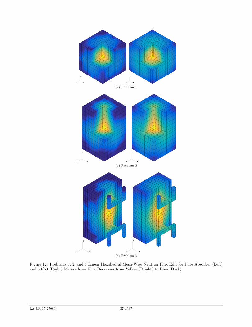
Also, isometric material distributions and flux edit results are created by converting the eeout files from
each execution to an XML-formatted unstructured mesh VTK file (Ref. 11) which is then displayed through
VisIt (Ref. 12) using its batch processing capabilities. The qualitative flux edits are presented to (a) provide
LA-UR-15-27089 7 of 37

an overall view of the flux behavior to validate its appropriateness and (b) illustrate one of the benefits
of using UM: minimal-overhead geometry-specific mesh-based results visualization. Only linear hexahedral
mesh results are shown here for demonstration purposes, but all other UM results appear similarly. However,
it should be noted that the coarse mesh generated with Attila4MC prevents appropriate interpretation of
the results. As such, the user is cautioned to specify the UM resolution considering both appropriate
representation of the geometry as well as the intended use of the UM edits.
IV.A. Problem 1
Results are reported in Reference 1 along three traverses in Problem 1, grouped and identified as Cases 1A,
1B, and 1C. Case 1A traverses every 10 cm in y from 5 to 95 cm, inclusive, keeping x = z = 5 cm. Case 1B
traverses along the diagonal with x = y = z = 5, 15, 25, . . . 95 cm. Case 1C traverses every 10 cm in x from
5 to 95 cm, inclusive, with y = 55 cm and z = 5 cm.
Results for Cases 1A, 1B, and 1C are shown in Figures 4, 5, and 6, respectively. For Cases 1A and
1C, CSG, Abaqus-generated UM, and Attila4MC-generated UM results agree with the Reference 1 solutions
within 1σ for pure absorber cases. For Case 1B, the UM results for the detector closest to the origin does
not agree within 2σ but is still within 3.5% of the benchmark value. For all cases with the 50/50 material
(most prominently in Case 1B), we see disagreement increasing as the detectors get further from the source.
This is a result of choosing to perform the calculations with only default variance reduction treatments.
Nevertheless, we can conclude that there is adequate statistical agreement between the various geometry
systems used and that they all produce results consistent with the reference solutions.
Note that for Case 1B, because the problem geometry is a cube, the point detectors lie on the interface
between adjacent elements when tetrahedral elements are used. In the course of performing this work,
significant effort was spent on improving the robustness of the UM particle tracking algorithms to not only
correctly handle this case but point detectors in general. Because of the potential for incorrect behavior,
users should exercise caution when using point detectors with UM when the detectors can lie on internal
UM interfaces for versions of MCNP6 before 6.1.2.
LA-UR-15-27089 8 of 37

IV.B. Problem 2
Results are reported in Reference 1 along two traverses in Problem 2, grouped and identified as Cases 2A
and 2B. Case 2A traverses every 10 cm in y from 5 to 95 cm, inclusive, keeping x = z = 5 cm. Case 2B
traverses every 10 cm in x from 5 to 55 cm, inclusive, with y = 95 cm and z = 5 cm.
Results for Cases 2A and 2B are shown in Figures 7 and 8, respectively. For pure absorber cases, 39 of
46 detectors agree with the reference solutions within 1σ (those other seven agree within 1.1σ). For 50/50
cases, 45 out of 46 detectors agree within 2σ. Similar to Problem 1, disagreement is primarily observed far
from the source which can be improved with additional variance reduction. Again we can conclude that
there is adequate statistical agreement between the various geometry systems used and that they all produce
results consistent with the reference solutions.
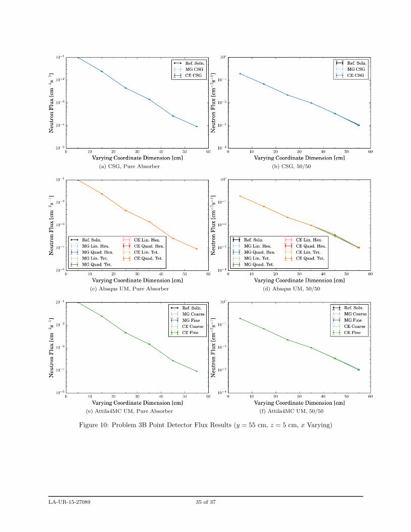
IV.C. Problem 3
Results are reported in Reference 1 along three traverses in Problem 3, grouped and identified as Cases 3A,
3B, and 3C. Case 3A traverses every 10 cm in y from 5 to 95 cm, inclusive, keeping x = z = 5 cm. Case 3B
traverses every 10 cm in x from 5 to 55 cm, inclusive, with y = 55 cm and z = 5 cm. Case 3C traverses
every 10 cm in x from 5 to 55 cm, inclusive, with y = 95 cm and z = 5 cm.
Results for Cases 3A, 3B, and 3C are shown in Figures 9, 10, and 11, respectively. Generally speaking,
the poorest agreement between the calculations performed herein and the benchmark values is observed for
this geometry. This is reasonable because the dogleg ducts represent a classic variance reduction problem
that hasn’t been explicitly addressed in this analysis. This behavior is also observed in Reference 3 despite
applying variance reduction. Nevertheless, for Cases 3A and 3B agreement between the calculated values
and the benchmark solutions is within 2σ or 5%. For Case 3C, agreement between the calculated values
and the benchmark solutions is within 2σ or 10%. In all cases, the results follow the trends observed in the
benchmark solutions.
LA-UR-15-27089 9 of 37

IV.D. Execution Time Discussion
In order to calculate the execution time, each calculation prints a timestamp immediately before and after
the calculation is performed. A Python-based script then parses the timestamps and calculates the difference
to the nearest second. The script then parses the number of particles used (from MCNP6’s nps variable)
and the number of processors used (because some calculations are more time consuming than others and
thus require more processors to fit within the execution wall clock time limits imposed by the queue system)
to calculate an aggregate speed which corresponds to the number of histories run per second per processor.
Note that this approach also accounts for non-transport related activities such as problem setup and output
file generation unlike the MCNP6-generated “source particles per minute” output; however, both approaches
show similar trends. Regardless, this approach is expected to provide a reasonable “real-world” measure of
relative speed between the various input permutations analyzed. See Tables IV – IX.
Several observations can be made regarding the speed results. First, CSG is faster than UM in all cases.
This is a widely recognized fact for simple problems given the general disparity in the total number of sur-
faces. However, it is clear that the speed to create models correctly representing complex geometry and the
clarity that unstructured mesh-based results can be visualized with cannot be overlooked when considering
total analysis time. We also see approximately two orders of magnitude in execution speed difference when
comparing different geometry types for a particular material configuration. Generally, hexahedron-based
UM are faster than equivalently-seeded tetrahedron-based UM (though total element count strongly drives
performance so the number of elements used should be minimized). Furthermore, linear elements are gen-
erally faster than quadratic elements. This illustrates the importance of selecting the appropriate element
type and degree of mesh refinement to balance accuracy and speed. Finally, MG cross sections tend to be
slightly faster than CE (1% ± 2%). However, like CSG versus UM, the time to create the data files should
be taken into consideration as well as the ability to work with them during post-processing.
LA-UR-15-27089 10 of 37

V. Conclusions
For all geometries, cross section energy treatments, and materials the calculated results herein followed the
behavior of the Reference 1 solutions. At worst, the results agreed within 2σ or 10% but generally within
1σ or 5%. Based on scoping studies and prior analyses, this agreement is expected to improve significantly
when additional variance reduction techniques are applied. By forgoing variance reduction in the calculations
herein, we are able to develop a sense of the results that are obtained when running with only the default
treatments and increase confidence that MCNP6’s UM tracking and interaction with point detectors produces
correct results.
In addition, we can develop fair comparisons of speed between different geometries and cross section
energy treatments. We have observed that: CSG calculations complete ∼10 times faster than the comparable
fastest UM calculations, there are only minor speed differences (∼1%) between MG and CE nuclear data,
there are significant speed differences (factor ∼100) between different element types for otherwise equivalent
calculations.
As such, it is recommended that users run with the simplest element type that adequately represents the
problem geometry, which are ideally first-order hexahedral elements. There is not a significant difference
in speed when using MG or CE cross sections, so it is recommended to use the best suited cross-section
libraries. Finally, the user is cautioned to examine point detector locations relative to element boundaries
to ensure that the detectors are not coincident with the boundaries, particularly for MCNP6 versions before
6.1.2.
Future work includes performing equivalent analyses with first- and second-order pentahedral elements.
This is not done in the present work because these elements tend to be used much less frequently than tetra-
and hexahedral elements. Furthermore, because of the desire to compare timing and results on an entirely
consistent basis, significant variance reduction is not performed herein. It would be interesting to examine
the effect of a consistent variance reduction scheme for equivalent problems.
LA-UR-15-27089 11 of 37

Acknowledgements
The authors wish to thank Gregory A. Failla and Ian M. Davis of Varian Medical Systems for providing the
licenses and expert insights that permitted the use of SpaceClaim and Attila4MC for this work.
LA-UR-15-27089 12 of 37

VI. References
[1] K. Kobayashi, N. Sugimura, and Y. Nagaya, “3-D Radiation Transport Benchmark Problems and Results
for Simple Geometries with Void Regions,” Tech. Rep. NEA/NSC/DOC(2000), NEA/OECD, Paris,
France, 2000.
[2] T. Mori and M. Nakagawa, “MVP/GMVP: General Purpose Monte Carlo Codes for Neutron and
Photon Transport Calculations based on Continuous Energy and Multigroup Methods,” Tech. Rep.
JAERI-Data/Code 94-007, Japan Atomic Energy Research Institute, Tokai-mura, Naka-gun, Ibaraki-
ken, Japan, 1994.
[3] B. Toth and F. B. Brown, “MCNP5 Benchmark Calculatiosn for 3-D Radiation Transport in Simple
Geometries with Void Regions,” Tech. Rep. LA-UR-03-5974, Los Alamos National Laboratory, Los
Alamos, NM, USA, 2003.
[4] J. T. Goorley et. al., “Initial MCNP6 Release Overview — MCNP6 version 1.0,” Tech. Rep. LA-UR-
13-22934, Los Alamos National Laboratory, Los Alamos, NM, USA, 2013.
[5] Dassault Systèmes Simulia Corp., “Abaqus/CAE 6.12 Online Documentation,” 2012.
[6] R. L. Martz, “The MCNP6 Book on Unstructured Mesh Geometry: User’s Guide,” Tech. Rep. LA-UR-
11-05668 Rev 8, Los Alamos National Laboratory, Los Alamos, NM, USA, 2014.
[7] J. A. Kulesza and R. L. Martz, “MCNP6 Unstructured Mesh Tutorial Using Abaqus/CAE 6.12-1,”
Tech. Rep. LA-UR-15-25143, Los Alamos National Laboratory, Los Alamos, NM, USA, 2015.
[8] Varian Medical Systems, “Attila with MCNP Integration: Attila4MC.” http://www.transpireinc.
com/html/attila, 2015. Accessed: 2015-08-25.
[9] F. B. Brown. Private Communication, 2015.
[10] C. A. Brewer, “Color Brewer 2.” http://www.colorbrewer2.org/. Accessed: 2015-08-10.
[11] W. J. Schroeder, K. M. Martin, and W. E. Lorensen, The Visualization Toolkit: An Object-Oriented
Approach to 3D Graphics. 4 ed., 2006.
LA-UR-15-27089 13 of 37

[12] H. Childs et. al., “VisIt: An End-User Tool For Visualizing and Analyzing Very Large Data,” in High
Performance Visualization — Enabling Extreme-Scale Scientific Insight, pp. 357–372, Oct 2012.
LA-UR-15-27089 14 of 37

Tables
I Problem 1 Unstructured Mesh Node & Element Counts
II Problem 2 Unstructured Mesh Node & Element Counts
III Problem 3 Unstructured Mesh Node & Element Counts
IV Problem 1 Multigroup Calculation Speed of Execution [Speed = Histories / (Second × Pro-
cessor), Higher is Better]
V Problem 1 Continuous Energy Calculation Speed of Execution [Speed = Histories / (Sec-
ond × Processor), Higher is Better]
VI Problem 2 Multigroup Calculation Speed of Execution [Speed = Histories / (Second × Pro-
cessor), Higher is Better]
VII Problem 2 Continuous Energy Calculation Speed of Execution [Speed = Histories / (Sec-
ond × Processor), Higher is Better]
VIII Problem 3 Multigroup Calculation Speed of Execution [Speed = Histories / (Second × Pro-
cessor), Higher is Better]
IX Problem 3 Continuous Energy Calculation Speed of Execution [Speed = Histories / (Sec-
ond × Processor), Higher is Better]
LA-UR-15-27089 15 of 37

Table I: Problem 1 Unstructured Mesh Node & Element Counts
Mesher Element Type Nodes Elements
Abaqus
First-Order Tetrahedrons 3422 17430Second-Order Tetrahedrons 25137 17430First-Order Hexahedrons 2197 1728Second-Order Hexahedrons 8281 1728
Attila4MC First-Order Tetrahedrons (Coarse) 89 228First-Order Tetrahedrons (Fine) 16442 60633
LA-UR-15-27089 16 of 37

Table II: Problem 2 Unstructured Mesh Node & Element Counts
Mesher Element Type Nodes Elements
Abaqus
First-Order Tetrahedrons 1412 6668Second-Order Tetrahedrons 10003 6668First-Order Hexahedrons 1053 768Second-Order Hexahedrons 3897 768
Attila4MC First-Order Tetrahedrons (Coarse) 63 112First-Order Tetrahedrons (Fine) 5020 22316
LA-UR-15-27089 17 of 37

Table III: Problem 3 Unstructured Mesh Node & Element Counts
Mesher Element Type Nodes Elements
Abaqus
First-Order Tetrahedrons 5809 30791Second-Order Tetrahedrons 43656 30791First-Order Hexahedrons 3549 2880Second-Order Hexahedrons 13481 2880
Attila4MC First-Order Tetrahedrons (Coarse) 385 1050First-Order Tetrahedrons (Fine) 7256 31973
LA-UR-15-27089 18 of 37

Table IV: Problem 1 Multigroup Calculation Speed of Execution [Speed = Histories / (Second × Processor),Higher is Better]
Speed Geometry Material2830 CSG 50/50919 CSG Pure Abs.455 Abaqus, Lin. Hex. 50/50246 Abaqus, Lin. Tet. 50/50211 Attila4MC, Coarse Pure Abs.186 Abaqus, Lin. Hex. Pure Abs.116 Attila4MC, Coarse 50/5069 Attila4MC, Fine Pure Abs.68 Abaqus, Lin. Tet. Pure Abs.39 Abaqus, Quad. Hex. Pure Abs.35 Attila4MC, Fine 50/5020 Abaqus, Quad. Tet. Pure Abs.16 Abaqus, Quad. Hex. 50/509 Abaqus, Quad. Tet. 50/50
LA-UR-15-27089 19 of 37

Table V: Problem 1 Continuous Energy Calculation Speed of Execution [Speed = Histories / (Second × Pro-cessor), Higher is Better]
Speed Geometry Material2741 CSG 50/501116 CSG Pure Abs.450 Abaqus, Lin. Hex. 50/50244 Abaqus, Lin. Tet. 50/50217 Attila4MC, Coarse Pure Abs.177 Abaqus, Lin. Hex. Pure Abs.114 Attila4MC, Coarse 50/5069 Attila4MC, Fine Pure Abs.67 Abaqus, Lin. Tet. Pure Abs.39 Abaqus, Quad. Hex. Pure Abs.35 Attila4MC, Fine 50/5020 Abaqus, Quad. Tet. Pure Abs.16 Abaqus, Quad. Hex. 50/509 Abaqus, Quad. Tet. 50/50
LA-UR-15-27089 20 of 37

Table VI: Problem 2 Multigroup Calculation Speed of Execution [Speed = Histories / (Second × Processor),Higher is Better]
Speed Geometry Material5341 CSG 50/501420 CSG Pure Abs.1152 Abaqus, Lin. Hex. 50/50639 Abaqus, Lin. Tet. 50/50411 Attila4MC, Coarse Pure Abs.316 Attila4MC, Coarse 50/50244 Abaqus, Lin. Hex. Pure Abs.205 Abaqus, Lin. Tet. Pure Abs.169 Attila4MC, Fine Pure Abs.128 Attila4MC, Fine 50/5093 Abaqus, Quad. Hex. Pure Abs.55 Abaqus, Quad. Tet. Pure Abs.47 Abaqus, Quad. Hex. 50/5027 Abaqus, Quad. Tet. 50/50
LA-UR-15-27089 21 of 37

Table VII: Problem 2 Continuous Energy Calculation Speed of Execution [Speed = Histories / (Second × Pro-cessor), Higher is Better]
Speed Geometry Material4952 CSG 50/501953 CSG Pure Abs.1124 Abaqus, Lin. Hex. 50/50634 Abaqus, Lin. Tet. 50/50411 Attila4MC, Coarse Pure Abs.313 Attila4MC, Coarse 50/50244 Abaqus, Lin. Hex. Pure Abs.205 Abaqus, Lin. Tet. Pure Abs.153 Attila4MC, Fine Pure Abs.128 Attila4MC, Fine 50/5093 Abaqus, Quad. Hex. Pure Abs.55 Abaqus, Quad. Tet. Pure Abs.47 Abaqus, Quad. Hex. 50/5027 Abaqus, Quad. Tet. 50/50
LA-UR-15-27089 22 of 37

Table VIII: Problem 3 Multigroup Calculation Speed of Execution [Speed = Histories / (Second × Processor),Higher is Better]
Speed Geometry Material962 CSG 50/50868 CSG Pure Abs.567 Abaqus, Lin. Hex. 50/50261 Abaqus, Lin. Tet. 50/50205 Abaqus, Lin. Hex. Pure Abs.190 Attila4MC, Coarse Pure Abs.90 Attila4MC, Fine Pure Abs.88 Attila4MC, Coarse 50/5058 Attila4MC, Fine 50/5055 Abaqus, Quad. Hex. Pure Abs.54 Abaqus, Lin. Tet. Pure Abs.25 Abaqus, Quad. Hex. 50/5021 Abaqus, Quad. Tet. Pure Abs.12 Abaqus, Quad. Tet. 50/50
LA-UR-15-27089 23 of 37

Table IX: Problem 3 Continuous Energy Calculation Speed of Execution [Speed = Histories / (Second × Pro-cessor), Higher is Better]
Speed Geometry Material1201 CSG Pure Abs.945 CSG 50/50558 Abaqus, Lin. Hex. 50/50257 Abaqus, Lin. Tet. 50/50195 Abaqus, Lin. Hex. Pure Abs.190 Attila4MC, Coarse Pure Abs.90 Attila4MC, Fine Pure Abs.87 Attila4MC, Coarse 50/5058 Attila4MC, Fine 50/5055 Abaqus, Quad. Hex. Pure Abs.54 Abaqus, Lin. Tet. Pure Abs.25 Abaqus, Quad. Hex. 50/5021 Abaqus, Quad. Tet. Pure Abs.12 Abaqus, Quad. Tet. 50/50
LA-UR-15-27089 24 of 37

Figures
1 Problem 1 (Nested Cubes) with Nearest Octant Hidden; Source/Shield Material: Dark, Void
Material: Light
2 Problem 2 (Straight Void Duct) with Nearest Octant Hidden; Source/Shield Material: Dark,
Void Material: Light
3 Problem 3 (Dogleg Void Duct) with Nearest Half-space Source/Shield Hidden; Source/Shield
Material: Dark, Void Material: Light
4 Problem 1A Point Detector Flux Results (x = z = 5 cm, y Varying)
5 Problem 1B Point Detector Flux Results (x = y = z Varying)
6 Problem 1C Point Detector Flux Results (y = 55 cm, z = 5 cm, x Varying)
7 Problem 2A Point Detector Flux Results (x = z = 5 cm, y Varying)
8 Problem 2B Point Detector Flux Results (y = 95 cm, z = 5 cm, x Varying)
9 Problem 3A Point Detector Flux Results (x = z = 5 cm, y Varying)
10 Problem 3B Point Detector Flux Results (y = 55 cm, z = 5 cm, x Varying)
11 Problem 3C Point Detector Flux Results (x = z = 5 cm, y Varying)
12 Problems 1, 2, and 3 Linear Hexahedral Mesh-Wise Neutron Flux Edit for Pure Absorber
(Left) and 50/50 (Right) Materials — Flux Decreases from Yellow (Bright) to Blue (Dark)
LA-UR-15-27089 25 of 37

(a) Tetrahedral (Left) and Hexahedral (Right) Abaqus-generatedUM
(b) Coarse (Left) and Fine (Right) Attila4MC-generated UM
Figure 1: Problem 1 (Nested Cubes) with Nearest Octant Hidden; Source/Shield Material: Dark, VoidMaterial: Light
LA-UR-15-27089 26 of 37

(a) Tetrahedral (Left) and Hexahedral (Right) Abaqus-generatedUM
(b) Coarse (Left) and Fine (Right) Attila4MC-generated UM
Figure 2: Problem 2 (Straight Void Duct) with Nearest Octant Hidden; Source/Shield Material: Dark, VoidMaterial: Light
LA-UR-15-27089 27 of 37

(a) Tetrahedral (Left) and Hexahedral (Right) Abaqus-generatedUM
(b) Coarse (Left) and Fine (Right) Attila4MC-generated UM
Figure 3: Problem 3 (Dogleg Void Duct) with Nearest Half-space Source/Shield Hidden; Source/ShieldMaterial: Dark, Void Material: Light
LA-UR-15-27089 28 of 37

(a) CSG, Pure Absorber (b) CSG, 50/50
(c) Abaqus UM, Pure Absorber (d) Abaqus UM, 50/50
(e) Attila4MC UM, Pure Absorber (f) Attila4MC UM, 50/50
Figure 4: Problem 1A Point Detector Flux Results (x = z = 5 cm, y Varying)
LA-UR-15-27089 29 of 37

(a) CSG, Pure Absorber (b) CSG, 50/50
(c) Abaqus UM, Pure Absorber (d) Abaqus UM, 50/50
(e) Attila4MC UM, Pure Absorber (f) Attila4MC UM, 50/50
Figure 5: Problem 1B Point Detector Flux Results (x = y = z Varying)
LA-UR-15-27089 30 of 37

(a) CSG, Pure Absorber (b) CSG, 50/50
(c) Abaqus UM, Pure Absorber (d) Abaqus UM, 50/50
(e) Attila4MC UM, Pure Absorber (f) Attila4MC UM, 50/50
Figure 6: Problem 1C Point Detector Flux Results (y = 55 cm, z = 5 cm, x Varying)
LA-UR-15-27089 31 of 37

(a) CSG, Pure Absorber (b) CSG, 50/50
(c) Abaqus UM, Pure Absorber (d) Abaqus UM, 50/50
(e) Attila4MC UM, Pure Absorber (f) Attila4MC UM, 50/50
Figure 7: Problem 2A Point Detector Flux Results (x = z = 5 cm, y Varying)
LA-UR-15-27089 32 of 37

(a) CSG, Pure Absorber (b) CSG, 50/50
(c) Abaqus UM, Pure Absorber (d) Abaqus UM, 50/50
(e) Attila4MC UM, Pure Absorber (f) Attila4MC UM, 50/50
Figure 8: Problem 2B Point Detector Flux Results (y = 95 cm, z = 5 cm, x Varying)
LA-UR-15-27089 33 of 37

(a) CSG, Pure Absorber (b) CSG, 50/50
(c) Abaqus UM, Pure Absorber (d) Abaqus UM, 50/50
(e) Attila4MC UM, Pure Absorber (f) Attila4MC UM, 50/50
Figure 9: Problem 3A Point Detector Flux Results (x = z = 5 cm, y Varying)
LA-UR-15-27089 34 of 37
(a) CSG, Pure Absorber (b) CSG, 50/50
(c) Abaqus UM, Pure Absorber (d) Abaqus UM, 50/50
(e) Attila4MC UM, Pure Absorber (f) Attila4MC UM, 50/50
Figure 10: Problem 3B Point Detector Flux Results (y = 55 cm, z = 5 cm, x Varying)
LA-UR-15-27089 35 of 37

(a) CSG, Pure Absorber (b) CSG, 50/50
(c) Abaqus UM, Pure Absorber (d) Abaqus UM, 50/50
(e) Attila4MC UM, Pure Absorber (f) Attila4MC UM, 50/50
Figure 11: Problem 3C Point Detector Flux Results (x = z = 5 cm, y Varying)
LA-UR-15-27089 36 of 37
(a) Problem 1
(b) Problem 2
(c) Problem 3
Figure 12: Problems 1, 2, and 3 Linear Hexahedral Mesh-Wise Neutron Flux Edit for Pure Absorber (Left)and 50/50 (Right) Materials — Flux Decreases from Yellow (Bright) to Blue (Dark)
LA-UR-15-27089 37 of 37