Lab 7: Tables Operations in ArcMap - GIS Courses 7: Tables Operations in ArcMap ... Most spatial data in a GIS consist of at least two types of data, ... Join Tables) In Arcmap,

GIS Fundamentals Lab 7 Table Operations

1

Lab 7: Tables Operations in ArcMap

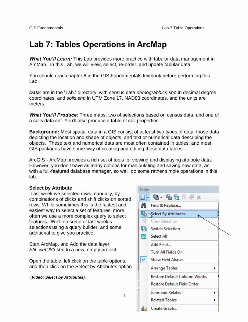
What You’ll Learn: This Lab provides more practice with tabular data management in ArcMap. In this Lab, we will view, select, re-order, and update tabular data. You should read chapter 8 in the GIS Fundamentals textbook before performing this Lab. Data: are in the \Lab7 directory, with census data demographics.shp in decimal degree coordinates, and soils.shp in UTM Zone 17, NAD83 coordinates, and the units are meters. What You’ll Produce: Three maps, two of selections based on census data, and one of a soils data set. You’ll also produce a table of soil properties. Background: Most spatial data in a GIS consist of at least two types of data, those data depicting the location and shape of objects, and text or numerical data describing the objects. These text and numerical data are most often contained in tables, and most GIS packages have some way of creating and editing these data tables. ArcGIS - ArcMap provides a rich set of tools for viewing and displaying attribute data. However, you don’t have as many options for manipulating and saving new data, as with a full-featured database manager, so we’ll do some rather simple operations in this lab. Select by Attribute Last week we selected rows manually, by combinations of clicks and shift clicks on sorted rows. While sometimes this is the fastest and easiest way to select a set of features, more often we use a more complex query to select features. We’ll do some of last week’s selections using a query builder, and some additional to give you practice. Start ArcMap, and Add the data layer Stil_wetU83.shp to a new, empty project. Open the table, left click on the table options, and then click on the Select by Attributes option (Video: Select by Attributes).


2

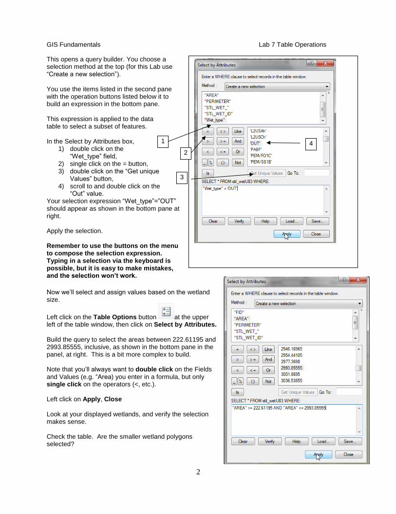
This opens a query builder. You choose a selection method at the top (for this Lab use “Create a new selection”). You use the items listed in the second pane with the operation buttons listed below it to build an expression in the bottom pane. This expression is applied to the data table to select a subset of features. In the Select by Attributes box,

1) double click on the “Wet_type” field,

2) single click on the = button, 3) double click on the “Get unique

Values” button, 4) scroll to and double click on the

“Out” value. Your selection expression “Wet_type”=”OUT” should appear as shown in the bottom pane at right. Apply the selection. Remember to use the buttons on the menu to compose the selection expression. Typing in a selection via the keyboard is possible, but it is easy to make mistakes, and the selection won’t work.

Now we’ll select and assign values based on the wetland size.

Left click on the Table Options button at the upper left of the table window, then click on Select by Attributes. Build the query to select the areas between 222.61195 and 2993.85555, inclusive, as shown in the bottom pane in the panel, at right. This is a bit more complex to build. Note that you’ll always want to double click on the Fields and Values (e.g. “Area) you enter in a formula, but only single click on the operators (<, etc.). Left click on Apply, Close Look at your displayed wetlands, and verify the selection makes sense. Check the table. Are the smaller wetland polygons selected?

1

2

4

3


3

If not, check your expression, and fix any errors. Right click on the “Size” column, then open the Field Calculator, and assign a “Size” values for the selected records to “Small”. Do the same steps as above for the "AREA" >= 3001.8695 AND "AREA" <= 9969.29615, use the Field Calculator to assign a value of “Medium” in the Size field for these records. Repeat the process for "AREA" >= 10076.1794 AND "AREA" <= 5103526.79121 OR “AREA” = 95146516.60342. Assign a value of “Large” to the Size field for the selected records. Finally, with the data table still open, select OptionsSelect by Attributes, select the Wet_type = “U” and use the Field Calculator to change that record’s value in the Size field to “Uplands”. Clear Selected Features (on the main ArcMap menu, under Selection).

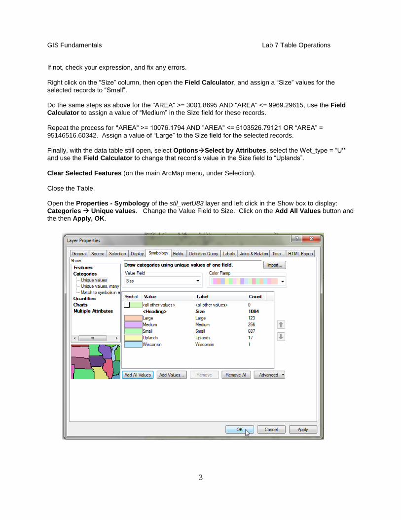
Close the Table. Open the Properties - Symbology of the stil_wetU83 layer and left click in the Show box to display: Categories Unique values. Change the Value Field to Size. Click on the Add All Values button and the then Apply, OK.


4

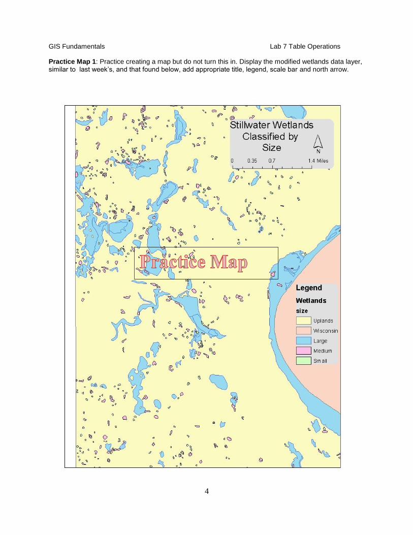
Practice Map 1: Practice creating a map but do not turn this in. Display the modified wetlands data layer, similar to last week’s, and that found below, add appropriate title, legend, scale bar and north arrow.


5

Wetlands Tables We’ll now assign a new column to identify general wetland types, based on recurrent selections. Create an ArcMap project, and add the shapefile Stil_wetU83. Right click on Stil_wetU83 in the TOC, and left click on Open Attribute Table. The field, or item, named “Wet_type” contains the wetland classification used by the US Fish and Wildlife Service. A complete list is found at the end of this lab exercise.

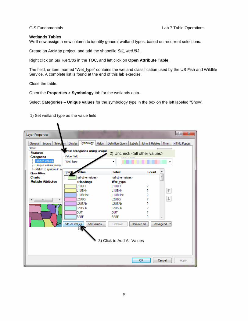
Close the table. Open the Properties > Symbology tab for the wetlands data. Select Categories – Unique values for the symbology type in the box on the left labeled “Show”.

1) Set wetland type as the value field

2) Uncheck <all other values>

3) Click to Add All Values


6

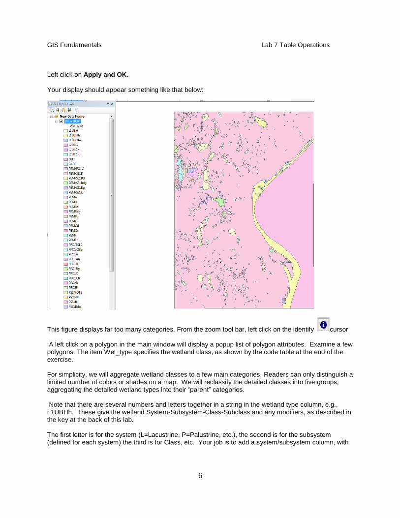
Left click on Apply and OK. Your display should appear something like that below:

This figure displays far too many categories. From the zoom tool bar, left click on the identify cursor A left click on a polygon in the main window will display a popup list of polygon attributes. Examine a few polygons. The item Wet_type specifies the wetland class, as shown by the code table at the end of the exercise. For simplicity, we will aggregate wetland classes to a few main categories. Readers can only distinguish a limited number of colors or shades on a map. We will reclassify the detailed classes into five groups, aggregating the detailed wetland types into their “parent” categories. Note that there are several numbers and letters together in a string in the wetland type column, e.g., L1UBHh. These give the wetland System-Subsystem-Class-Subclass and any modifiers, as described in the key at the back of this lab. The first letter is for the system (L=Lacustrine, P=Palustrine, etc.), the second is for the subsystem (defined for each system) the third is for Class, etc. Your job is to add a system/subsystem column, with


7

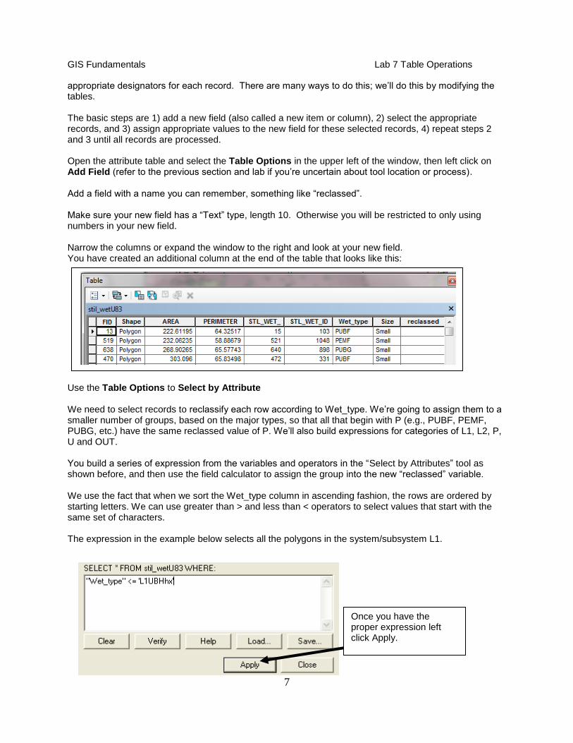
appropriate designators for each record. There are many ways to do this; we’ll do this by modifying the tables. The basic steps are 1) add a new field (also called a new item or column), 2) select the appropriate records, and 3) assign appropriate values to the new field for these selected records, 4) repeat steps 2 and 3 until all records are processed. Open the attribute table and select the Table Options in the upper left of the window, then left click on Add Field (refer to the previous section and lab if you’re uncertain about tool location or process).

Add a field with a name you can remember, something like “reclassed”. Make sure your new field has a “Text” type, length 10. Otherwise you will be restricted to only using numbers in your new field. Narrow the columns or expand the window to the right and look at your new field. You have created an additional column at the end of the table that looks like this:

Use the Table Options to Select by Attribute

We need to select records to reclassify each row according to Wet_type. We’re going to assign them to a smaller number of groups, based on the major types, so that all that begin with P (e.g., PUBF, PEMF, PUBG, etc.) have the same reclassed value of P. We’ll also build expressions for categories of L1, L2, P, U and OUT. You build a series of expression from the variables and operators in the “Select by Attributes” tool as shown before, and then use the field calculator to assign the group into the new “reclassed” variable. We use the fact that when we sort the Wet_type column in ascending fashion, the rows are ordered by starting letters. We can use greater than > and less than < operators to select values that start with the same set of characters. The expression in the example below selects all the polygons in the system/subsystem L1.

Once you have the proper expression left click Apply.


8

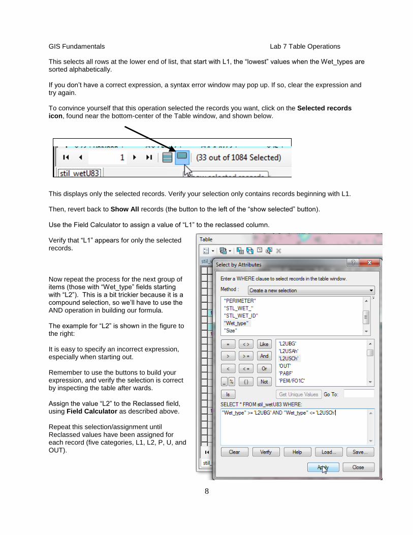
This selects all rows at the lower end of list, that start with L1, the “lowest” values when the Wet_types are sorted alphabetically. If you don’t have a correct expression, a syntax error window may pop up. If so, clear the expression and try again. To convince yourself that this operation selected the records you want, click on the Selected records icon, found near the bottom-center of the Table window, and shown below.

This displays only the selected records. Verify your selection only contains records beginning with L1. Then, revert back to Show All records (the button to the left of the “show selected” button). Use the Field Calculator to assign a value of “L1” to the reclassed column.

Verify that “L1” appears for only the selected records.

Now repeat the process for the next group of items (those with “Wet_type” fields starting with “L2”). This is a bit trickier because it is a compound selection, so we’ll have to use the AND operation in building our formula. The example for “L2” is shown in the figure to the right: It is easy to specify an incorrect expression, especially when starting out. Remember to use the buttons to build your expression, and verify the selection is correct by inspecting the table after wards. Assign the value “L2” to the Reclassed field, using Field Calculator as described above. Repeat this selection/assignment until Reclassed values have been assigned for each record (five categories, L1, L2, P, U, and OUT).


9

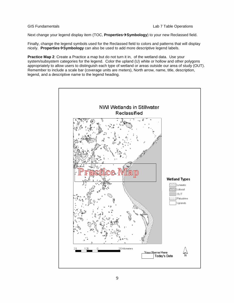
Next change your legend display item (TOC, PropertiesSymbology) to your new Reclassed field.

Finally, change the legend symbols used for the Reclassed field to colors and patterns that will display nicely. PropertiesSymbology can also be used to add more descriptive legend labels. Practice Map 2: Create a Practice a map but do not turn it in, of the wetland data. Use your system/subsystem categories for the legend. Color the upland (U) white or hollow and other polygons appropriately to allow users to distinguish each type of wetland or areas outside our area of study (OUT). Remember to include a scale bar (coverage units are meters), North arrow, name, title, description, legend, and a descriptive name to the legend heading.


10

Joining Two Existing Tables (Video: Join Tables) In Arcmap, create a new map, and Add the theme demographics.shp. Open the Attribute Table. Note the fields, especially one called Blkgrp. Add the data table name more_data.dbf, using Add Data (as you would add a layer). Right click on more_data.dbf in the TOC, and left click on Open Notice that more_data.dbf also has an item named Blkgrp. Use the scroll bars at the bottom of each table to look at all the variables (columns) in each table. Are the variables ordinal, nominal, or interval/ratio? Which variables are found in both tables? Which variables might serve as keys for the table, and which would be inappropriate as keys? See Chapter 8 in the textbook, if you’re unsure on these concepts. Each record (row) in each table corresponds to each polygon in this US Census Bureau demographic data, displayed in demographics.shp. These files were produced from U.S. Census data, which uses a variable named Blkgrp as unique identifiers, typically for groups of city blocks used to summarize census data. Each record in our tables corresponds to a block group. The file more_data.dbf includes populations at various dates for each block group polygon, e.g., Hh80=population in 1980, Hh90= population in 1990, etc.

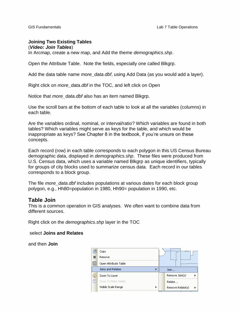
Table Join This is a common operation in GIS analyses. We often want to combine data from different sources. Right click on the demographics.shp layer in the TOC select Joins and Relates and then Join


11

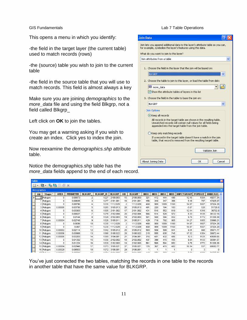
This opens a menu in which you identify: -the field in the target layer (the current table) used to match records (rows) -the (source) table you wish to join to the current table -the field in the source table that you will use to match records. This field is almost always a key Make sure you are joining demographics to the more_data file and using the field Blkgrp, not a field called Blkgrp_ Left click on OK to join the tables. You may get a warning asking if you wish to create an index. Click yes to index the join. Now reexamine the demographics.shp attribute table.

Notice the demographics.shp table has the more_data fields append to the end of each record.

You’ve just connected the two tables, matching the records in one table to the records in another table that have the same value for BLKGRP.


12

This is a temporary join; the original files/data have not been modified. ArcMap keeps track of joins within a project, and how to display the various joined files. If you were to display these data sets in another project, they would not appear joined. The data are not copied to a new, combined, file. Rather, this join tells ArcMap to display these two data sets within this particular view, matching each row by the join variable.

Selecting on a Joined Table Now, let’s select items based on the joined tables. (Video: Compound Select)

Open the Attributes Table of demographics. It should display both the original data plus the data from more_data.dbf.

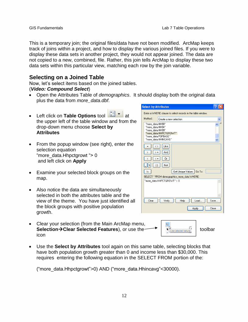
Left click on Table Options tool at the upper left of the table window and from the drop-down menu choose Select by Attributes

From the popup window (see right), enter the selection equation “more_data.Hhpctgrowt “> 0 and left click on Apply

Examine your selected block groups on the map.

Also notice the data are simultaneously selected in both the attributes table and the view of the theme. You have just identified all the block groups with positive population growth.

Clear your selection (from the Main ArcMap menu, SelectionClear Selected Features), or use the toolbar icon

Use the Select by Attributes tool again on this same table, selecting blocks that have both population growth greater than 0 and income less than $30,000. This requires entering the following equation in the SELECT FROM portion of the: (“more_data.Hhpctgrowt”>0) AND (“more_data.Hhincavg”<30000).


13

Click on Apply and examine your selection.

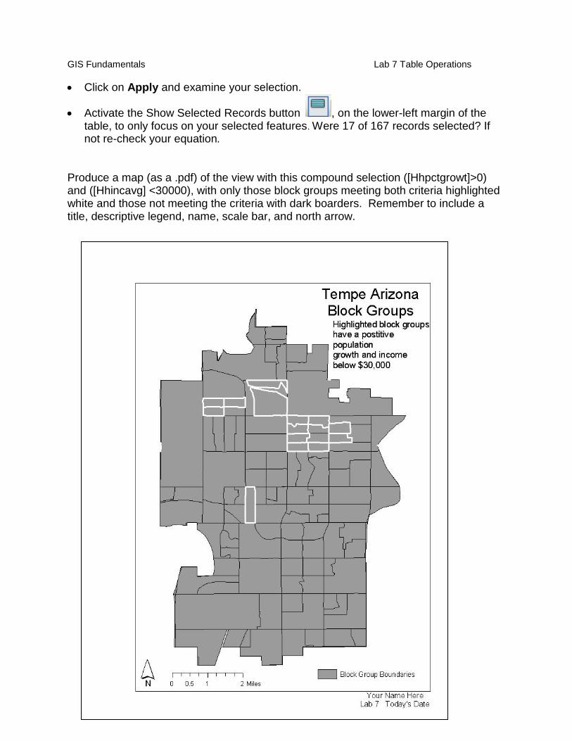
Activate the Show Selected Records button , on the lower-left margin of the table, to only focus on your selected features. Were 17 of 167 records selected? If not re-check your equation.

Produce a map (as a .pdf) of the view with this compound selection ([Hhpctgrowt]>0) and ([Hhincavg] <30000), with only those block groups meeting both criteria highlighted white and those not meeting the criteria with dark boarders. Remember to include a title, descriptive legend, name, scale bar, and north arrow.


14

Saving a Copy of a Joined Layer and Table

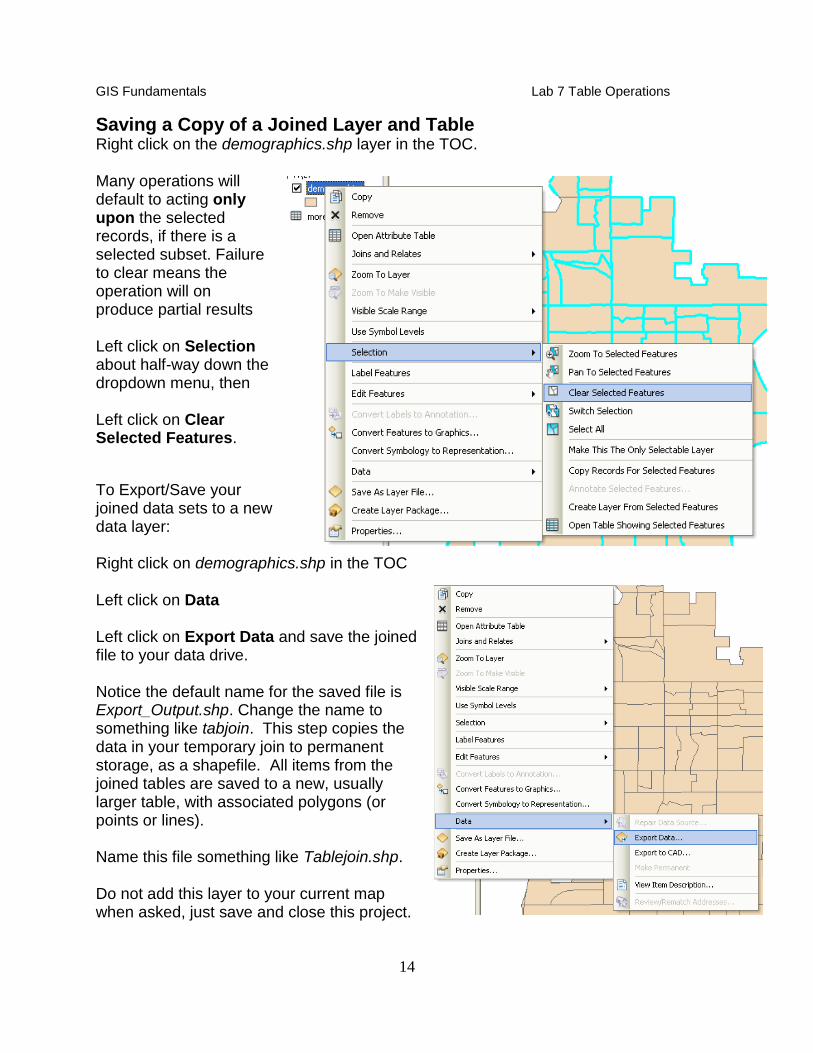
Right click on the demographics.shp layer in the TOC. Many operations will default to acting only upon the selected records, if there is a selected subset. Failure to clear means the operation will on produce partial results Left click on Selection about half-way down the dropdown menu, then Left click on Clear Selected Features.

To Export/Save your joined data sets to a new data layer: Right click on demographics.shp in the TOC Left click on Data Left click on Export Data and save the joined file to your data drive. Notice the default name for the saved file is Export_Output.shp. Change the name to something like tabjoin. This step copies the data in your temporary join to permanent storage, as a shapefile. All items from the joined tables are saved to a new, usually larger table, with associated polygons (or points or lines). Name this file something like Tablejoin.shp. Do not add this layer to your current map when asked, just save and close this project.


15

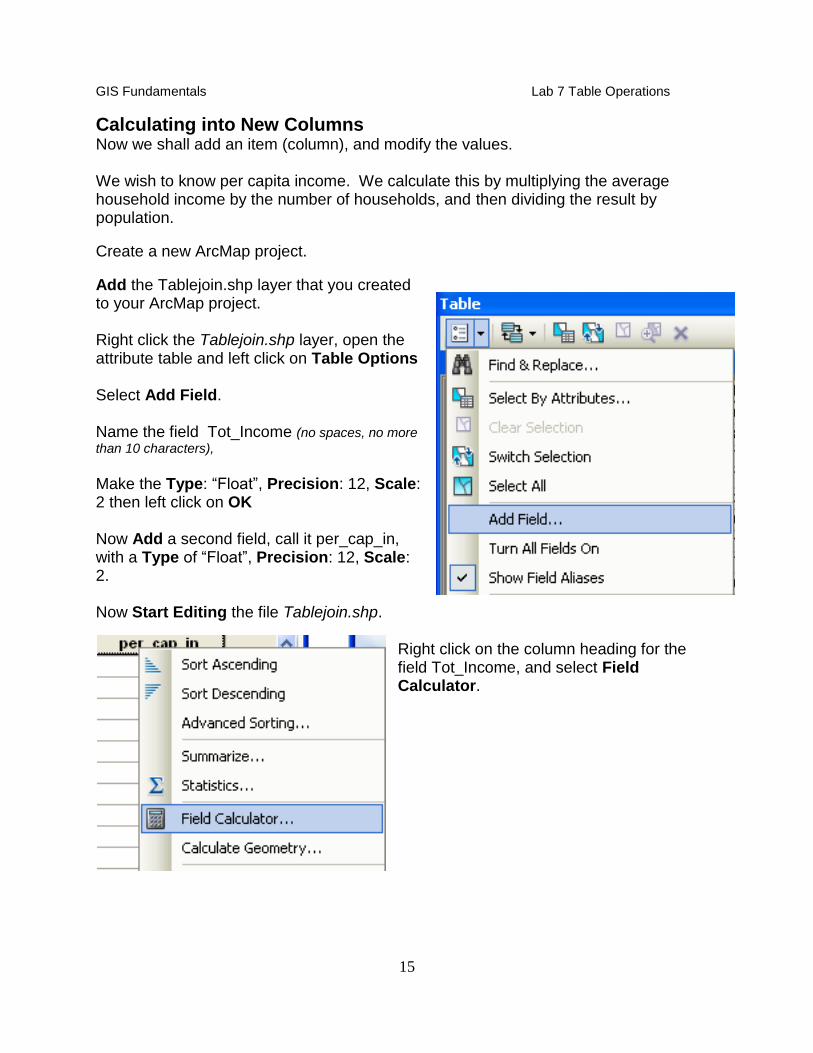
Calculating into New Columns Now we shall add an item (column), and modify the values. We wish to know per capita income. We calculate this by multiplying the average household income by the number of households, and then dividing the result by population.

Create a new ArcMap project.

Add the Tablejoin.shp layer that you created to your ArcMap project. Right click the Tablejoin.shp layer, open the attribute table and left click on Table Options Select Add Field. Name the field Tot_Income (no spaces, no more

than 10 characters), Make the Type: “Float”, Precision: 12, Scale: 2 then left click on OK Now Add a second field, call it per_cap_in, with a Type of “Float”, Precision: 12, Scale: 2. Now Start Editing the file Tablejoin.shp.

Right click on the column heading for the field Tot_Income, and select Field Calculator.


16

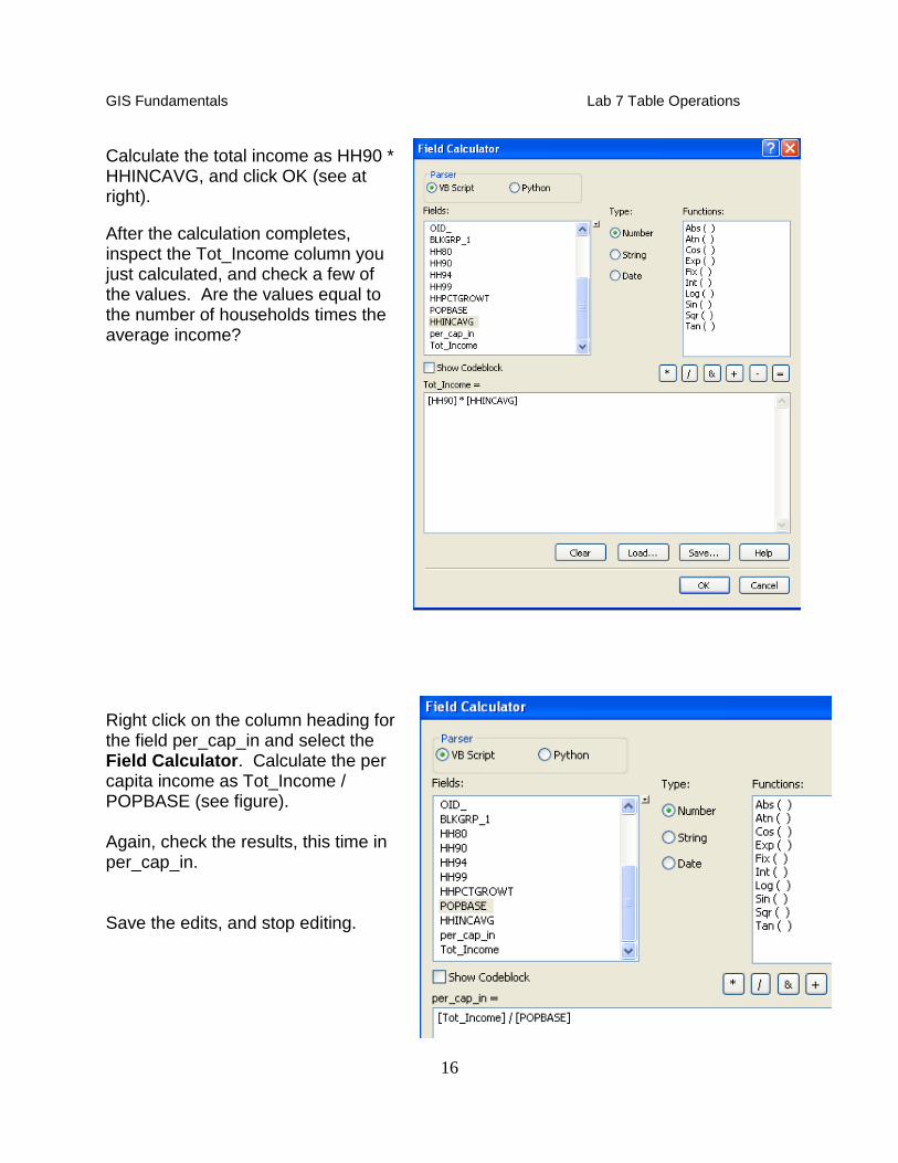
Calculate the total income as HH90 * HHINCAVG, and click OK (see at right).

After the calculation completes, inspect the Tot_Income column you just calculated, and check a few of the values. Are the values equal to the number of households times the average income? Right click on the column heading for the field per_cap_in and select the Field Calculator. Calculate the per capita income as Tot_Income / POPBASE (see figure). Again, check the results, this time in per_cap_in. Save the edits, and stop editing.


17

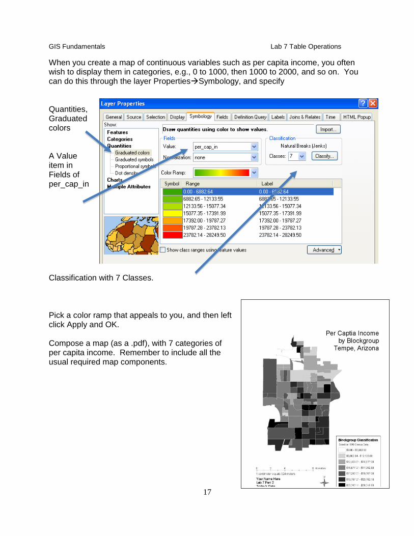
When you create a map of continuous variables such as per capita income, you often wish to display them in categories, e.g., 0 to 1000, then 1000 to 2000, and so on. You can do this through the layer PropertiesSymbology, and specify Quantities, Graduated colors A Value item in Fields of per_cap_in

Classification with 7 Classes. Pick a color ramp that appeals to you, and then left click Apply and OK. Compose a map (as a .pdf), with 7 categories of per capita income. Remember to include all the usual required map components.


18

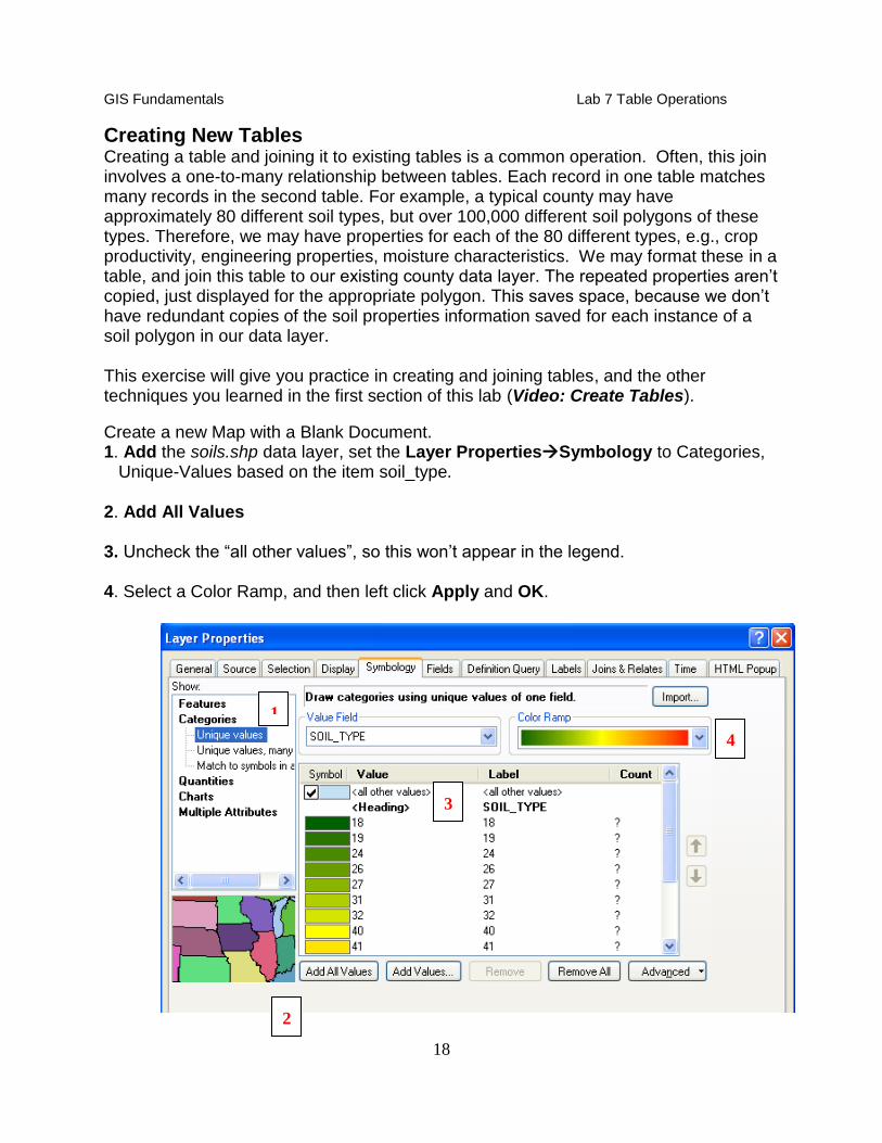
Creating New Tables Creating a table and joining it to existing tables is a common operation. Often, this join involves a one-to-many relationship between tables. Each record in one table matches many records in the second table. For example, a typical county may have approximately 80 different soil types, but over 100,000 different soil polygons of these types. Therefore, we may have properties for each of the 80 different types, e.g., crop productivity, engineering properties, moisture characteristics. We may format these in a table, and join this table to our existing county data layer. The repeated properties aren’t copied, just displayed for the appropriate polygon. This saves space, because we don’t have redundant copies of the soil properties information saved for each instance of a soil polygon in our data layer. This exercise will give you practice in creating and joining tables, and the other techniques you learned in the first section of this lab (Video: Create Tables). Create a new Map with a Blank Document. 1. Add the soils.shp data layer, set the Layer PropertiesSymbology to Categories, Unique-Values based on the item soil_type. 2. Add All Values 3. Uncheck the “all other values”, so this won’t appear in the legend. 4. Select a Color Ramp, and then left click Apply and OK.

Example suggestion

for Lab 7, Turn –In 2.

Be creative,

but include the

important information

1

2

3

4


19

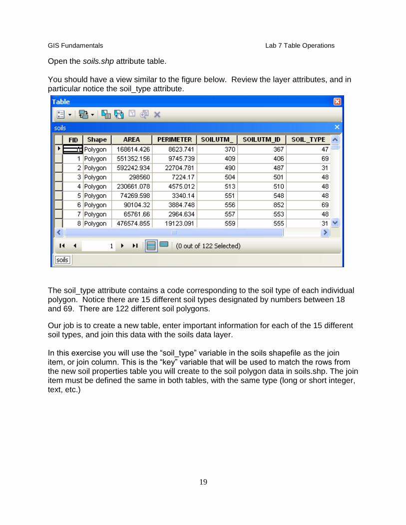
Open the soils.shp attribute table. You should have a view similar to the figure below. Review the layer attributes, and in particular notice the soil_type attribute.

The soil_type attribute contains a code corresponding to the soil type of each individual polygon. Notice there are 15 different soil types designated by numbers between 18 and 69. There are 122 different soil polygons.

Our job is to create a new table, enter important information for each of the 15 different soil types, and join this data with the soils data layer. In this exercise you will use the “soil_type” variable in the soils shapefile as the join item, or join column. This is the “key” variable that will be used to match the rows from the new soil properties table you will create to the soil polygon data in soils.shp. The join item must be defined the same in both tables, with the same type (long or short integer, text, etc.)


20

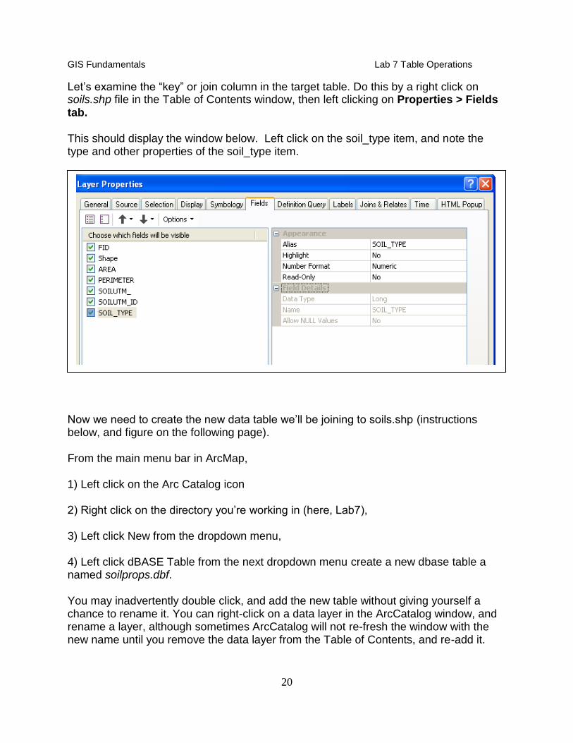
Let’s examine the “key” or join column in the target table. Do this by a right click on soils.shp file in the Table of Contents window, then left clicking on Properties > Fields tab. This should display the window below. Left click on the soil_type item, and note the type and other properties of the soil_type item.

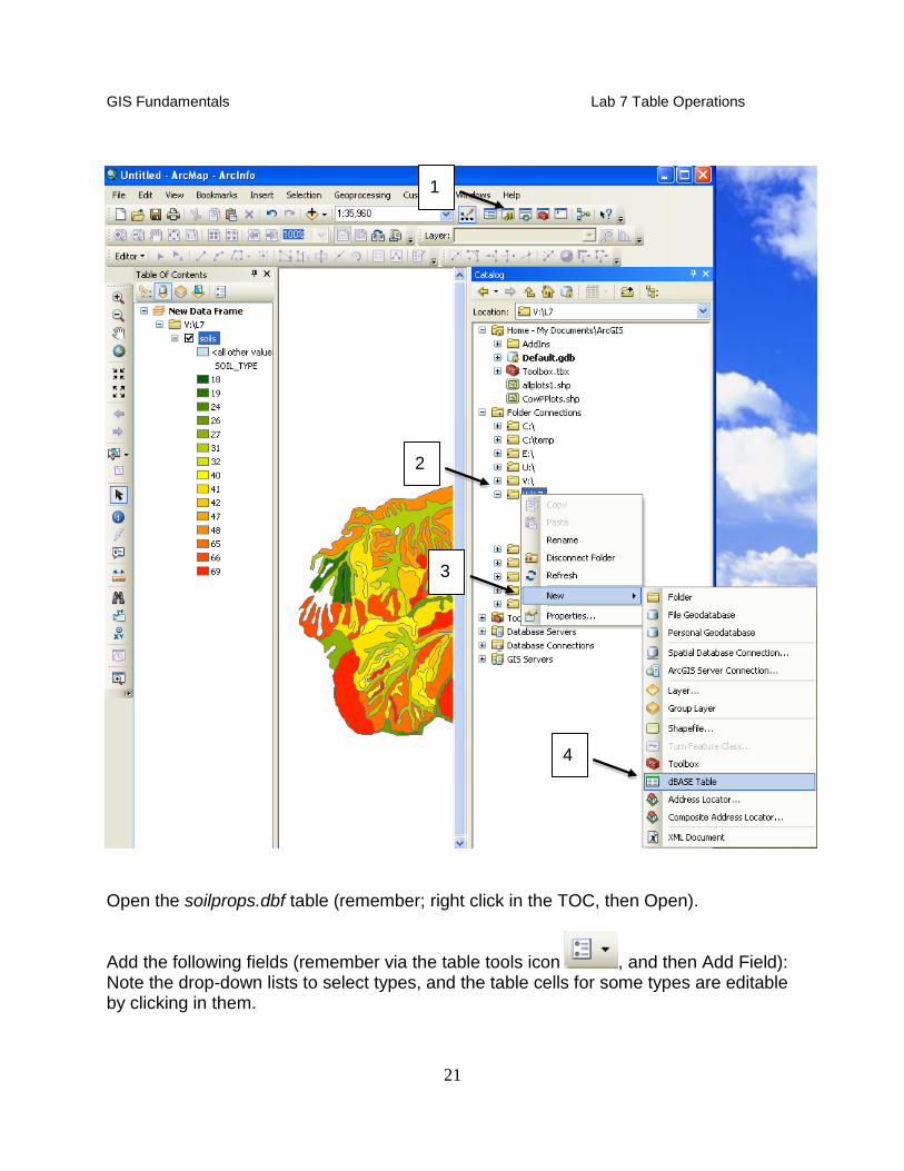
Now we need to create the new data table we’ll be joining to soils.shp (instructions below, and figure on the following page). From the main menu bar in ArcMap, 1) Left click on the Arc Catalog icon 2) Right click on the directory you’re working in (here, Lab7), 3) Left click New from the dropdown menu, 4) Left click dBASE Table from the next dropdown menu create a new dbase table a named soilprops.dbf. You may inadvertently double click, and add the new table without giving yourself a chance to rename it. You can right-click on a data layer in the ArcCatalog window, and rename a layer, although sometimes ArcCatalog will not re-fresh the window with the new name until you remove the data layer from the Table of Contents, and re-add it.


21

Open the soilprops.dbf table (remember; right click in the TOC, then Open).

Add the following fields (remember via the table tools icon , and then Add Field): Note the drop-down lists to select types, and the table cells for some types are editable by clicking in them.

1

2

3

4


22

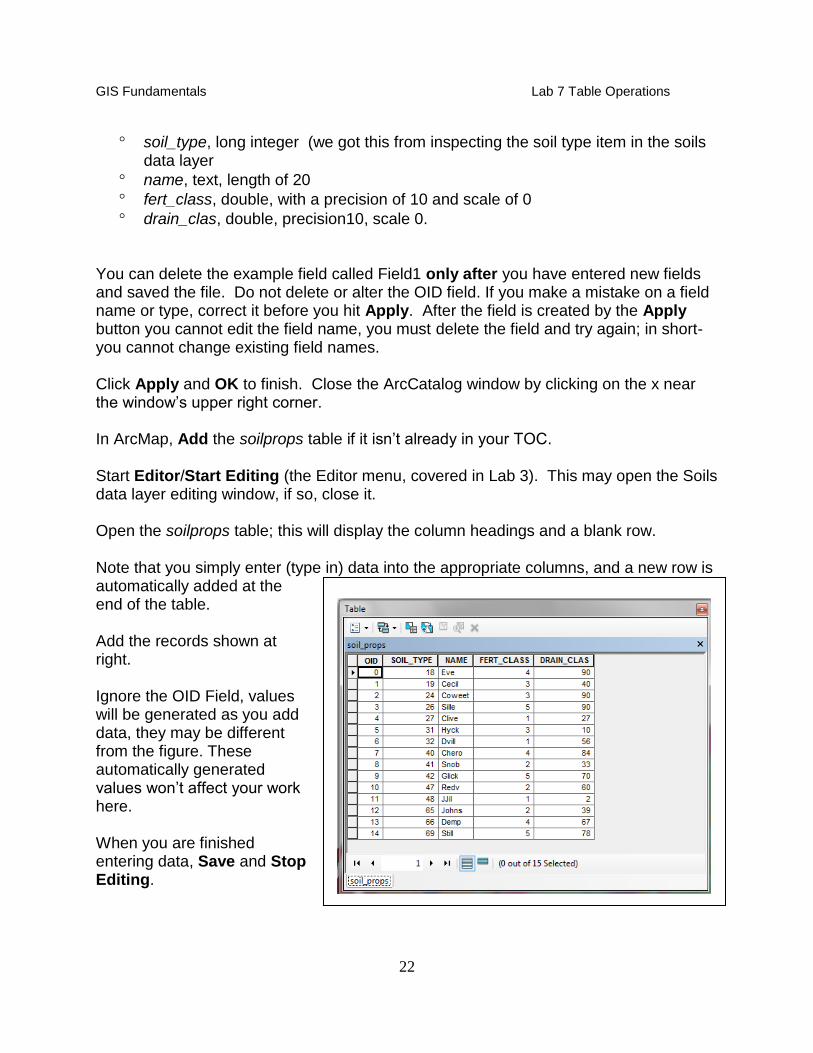
soil_type, long integer (we got this from inspecting the soil type item in the soils data layer

name, text, length of 20

fert_class, double, with a precision of 10 and scale of 0

drain_clas, double, precision10, scale 0.

You can delete the example field called Field1 only after you have entered new fields and saved the file. Do not delete or alter the OID field. If you make a mistake on a field name or type, correct it before you hit Apply. After the field is created by the Apply button you cannot edit the field name, you must delete the field and try again; in short- you cannot change existing field names. Click Apply and OK to finish. Close the ArcCatalog window by clicking on the x near the window’s upper right corner. In ArcMap, Add the soilprops table if it isn’t already in your TOC. Start Editor/Start Editing (the Editor menu, covered in Lab 3). This may open the Soils data layer editing window, if so, close it. Open the soilprops table; this will display the column headings and a blank row. Note that you simply enter (type in) data into the appropriate columns, and a new row is automatically added at the end of the table. Add the records shown at right. Ignore the OID Field, values will be generated as you add data, they may be different from the figure. These automatically generated values won’t affect your work here.

When you are finished entering data, Save and Stop Editing.


23

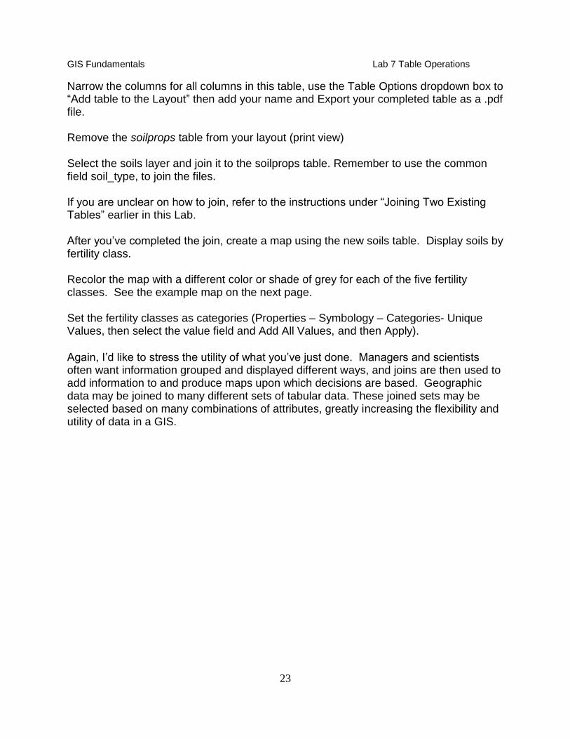
Narrow the columns for all columns in this table, use the Table Options dropdown box to “Add table to the Layout” then add your name and Export your completed table as a .pdf file. Remove the soilprops table from your layout (print view) Select the soils layer and join it to the soilprops table. Remember to use the common field soil_type, to join the files. If you are unclear on how to join, refer to the instructions under “Joining Two Existing Tables” earlier in this Lab. After you’ve completed the join, create a map using the new soils table. Display soils by fertility class. Recolor the map with a different color or shade of grey for each of the five fertility classes. See the example map on the next page. Set the fertility classes as categories (Properties – Symbology – Categories- Unique Values, then select the value field and Add All Values, and then Apply).

Again, I’d like to stress the utility of what you’ve just done. Managers and scientists often want information grouped and displayed different ways, and joins are then used to add information to and produce maps upon which decisions are based. Geographic data may be joined to many different sets of tabular data. These joined sets may be selected based on many combinations of attributes, greatly increasing the flexibility and utility of data in a GIS.


24

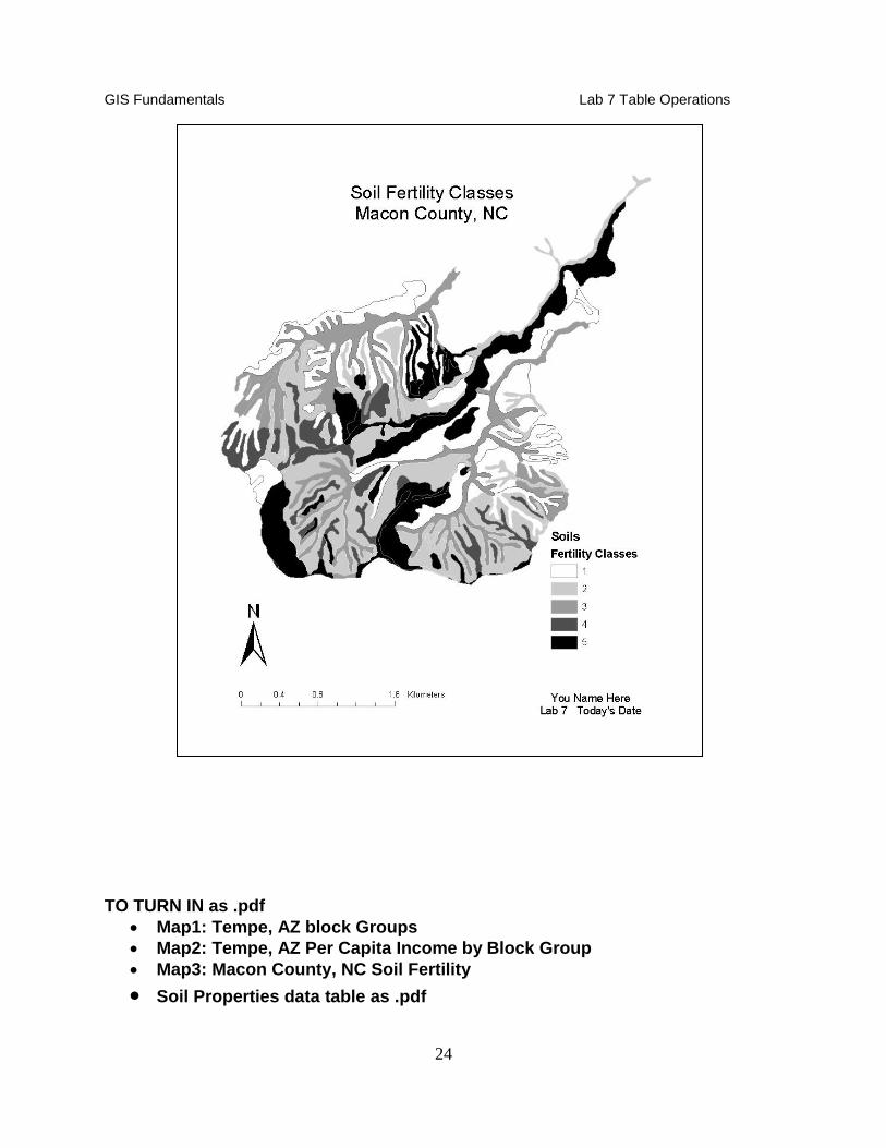
TO TURN IN as .pdf

Map1: Tempe, AZ block Groups

Map2: Tempe, AZ Per Capita Income by Block Group

Map3: Macon County, NC Soil Fertility

Soil Properties data table as .pdf

Documents

Lab 7: Tables Operations in ArcMap - GIS Courses 7: Tables Operations in ArcMap ... Most spatial data in a GIS consist of at least two types of data, ... Join Tables) In Arcmap,