AD-AI05 900 MASSACHUSETTS INST OF TECH CAMBRIDGE LAB FOR INFORMA-ETC F/6 9/2

DEVELOPMENT OF A METHODOLOGY FOR THE DETECTION OF SYSTEM FA ILUR--ETC(U)

JUL 81 A1 S WILLSKT. E Y CHOW NOOSDN 77-C 0224

UNCLASS IFIED LIDS-SR-1145 NL

EE~hEE~hhhh

October, 1980 LIDS-SR- 1145

!I

Laboratory for Information and Decision SystemsMassachusetts Institute of Technology

Cambridge, MA 02139

Status Report Number Five, On the' Development of a Methodology for theDetection of System Failures and-for the Design of Fault-Tolerant ControlSystems

ONR Contract No. N0OO14-77-C-0224 %,

October 1, 1980 through September 30, 1981

/ I

I

To: Dr. Charles HollandMathematics Program (Code 432) 31Office of Naval Research800 North Quincy Boulevard

;!Arlington, Virginia 22217

T'IApprove d tot ptublic release;

Di::triburtin Unlimited

-2-

SUMMARY

A brief description of the research carried out by faculty, staff,

and students of the M.I.T. Laboratory forknformation and Decision Systems

under ONR Contract N00014-77-C-0224 is described. The period covered in

this status report is from October 1, 1980 through September 30, 1981.

The scope of this contract is the development of an overall failure

detection system design methodology and of methods for fault-tolerant

control. In thel • " we overview the research that has been

performed in these areas during the indicated time period. We-tave-- also

im.i-uded a list of the papers and reports that have been and are being

written as a result of research performed under this contract. 1I-a di±.ion,

during the period mentioned above, Prof. Alan S. Willsky, principal investi-

gator for thi- ceLxact, visited the People's Republic of China and Japan.

A trip report was submitted to . Ieicathematics Proqgam (Code-432), and a

copy of that report is included as Appendix A to this status report.

Accession For

-NTIS GRA&I

DTIC TAB

Unannouncedcjust ifi4cvt o . . .. .

Distr Ltut ion/

Dist

-3-

I. Robust Comparison Signals for Failure Detection

As discussed in the preceding progress report [19] for this project,

a key problem is the development of methods for generating comparison

signals that can be used reliably to detect failures given the presence

of system parameter uncertainties. Previously we have made some initial

progress in this area, as is described in [191 and in more detail in the

Ph.D. dissertation of E.Y. Chow (81 and in the paper [161. In this work

we used the idea of redundancy relations which are simply algebraic re-

lationships among system outputs at several times. Using this concept,

we proposed an analytic method for determining the parameters defining a

comparison signal that is optimum in the sense of minimizing the influence

of parameter uncertainties on the value of the signal under normal operation.

This research represented a significant step in increasing our

understanding of robust failure detection and in development a useful,

complete methodology. There were, however, several key limitations to

this earlier work. Specifically,

(a) No algorithmic method existed for identifying and constructing

all possible redundancy relations for a given system.

(b) No method existed for constructing the set of redundancy

relations which can be used to detect a given failure.

More generally, no method existed for finding all sets

of redundancy relations which allow one to detect each

of a set of specified failures and to distinguish among

them.

(c) The optimization formulation developed is complex and its

use for systems of moderate size seemed prohibitive. Also,

the method leads to a choice of comparison signals that

depends upon the system state and input. While this may be

-4-

appropriate in some problems, it is not in many others.

Furthermore the formulation dealt primarily with minimizing

the influence of parameter uncertainties on comparison signals

under normal operation. No single, satisfactory formulation

existed for incorporating the performance of the particular

signal choice under both unfailed and failed system conditions.

(d) No coherent picture existed for describing the full range of

possible methods for using a particular redundancy relationship

and for quantitatively relating performance as measured by the

optimization criterion to an actual failure detection algorithm

based on the redundancy relation.

During this past year we have initiated a new, related research pro-

ject aimed at developing algebraic and geometric approaches to overcoming

these limitations. We have identified and begun to develop an extremely

promising approach. Our work to date will be described in some detail

in the forthcoming S.M. thesis proposal of Mr. Xi-Chang Lon [201. In

this section we will briefly outline the main ideas.

Consider a linear system of the form

x(k+l) = Ax(k) (1.1)

y~k] = Cx(k) (1.2)

For simplicity in our initial discussion here and in the first part of

our research we will not include inputs (and hence will focus on sensor

failures and not on actuator failures). Let y (k) denote an extended

observation vector of length p+l.

yp(k) = [y'(k), y'(k+l),..., y'(k+p)] (1.3)

Any vector

-.

-5-

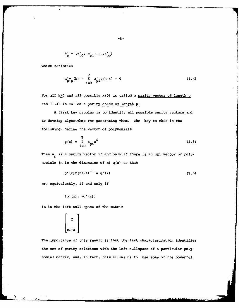
a' = (a0, a' ,...,a'p]p p0 p1 p

which satisfies

paly (k) = E apiy(k+i) =0 (1.4)

i=0

for all k>O and all possible x(0) is called a parity vector of length p

and (1.4) is called a parity check of length p.

A first key problem is to identify all possible parity vectors and

to develop algorithms for generating them. The key to this is the

following: define the vector of polynomials

Pp(z) = Z a .z (1.5)

i=0 p3

Then a is a parity vector if and only if there is an nxl vector of poly-p

nomials (n is the dimension of x) q(z) so that

-ip' (z)C (zI-A) = q' (z) (1.6)

or, equivalently, if and only if

[p'(z), -q'(z)]

is in the left null space of the matrix

The importance of this result is that the last characterization identifies

the set of parity relations with the left nullspace of a particular poly-

nomial matrix, and, in fact, this allows us to use some of the powerful

-6-

tools of the algebraic theory of linear systems to construct all possible

redundancy relations and, in fact, to find a basis consisting of parity

checks of minimal length. As length directly corresponds to the amount of

memory involved in a parity check one intuitively would prefer short

checks, in order to minimize the effects of parameter uncertainties.

Work is presently continuing in developing algorithms for constructing

parity checks and for finding parity vectors that are useful for particular

failure modes. Specifically, suppose that in addition to the normal operation

model (1.1), (1.2) we also have a set of possible failure models

x(k+l) = A.x(k) (1.7)1

y(k) = C.X(k) (1.8)1

i=l,... ,N. Suppose that a vector a is a valid parity vector, i.e. there

is a q(z) so that [p'(z), -q'(z)] is the left nullspace of

I (1. 9)3 I-A

ZICAJ

Suppose also that there is no polynomial q (z) so that [p' (z), -q!.(z)] isi1

in the left nullspace ofC.(1.10)

zI-A i

In this case the parity check (1.4) will give a value of zero if there is

no failure but will generally give a nonzero value if failure mode i

occurs. Clearly then what we wish to identify are the intersections of

the left nullspaces of the matrices in (1.9) and (1.10). As discussed in

-7-

[20] this can also be used to determine sets of parity checks which can

distinguish among a set of failures. Work is continuing on obtaining

algorithmic solutions.

The research described above is aimed directly at several of the

limitations mentioned earlier. Using the results of this research we have

also initiated research of a more geometric nature that is aimed at over-

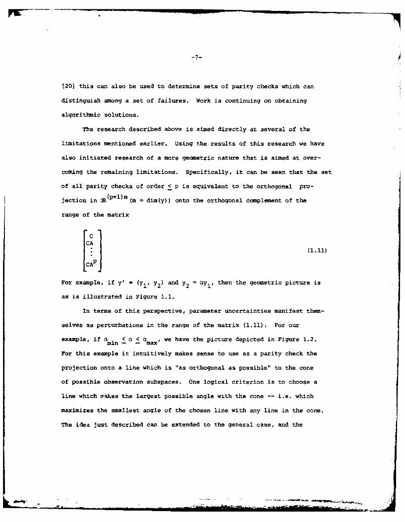
coming the remaining limitations. Specifically, it can be seen that the set

of all parity checks of order < p is equivalent to the orthogonal pro-

jection in 3R (p + ) m (m = dim(y)) onto the orthogonal complement of the

range of the matrix

iC1;CA

[CAPJ

For example, if y' = (yl' y2) and y2 = cY1 ' then the geometric picture is

as is illustrated in Figure 1.1.

In terms of this perspective, parameter uncertainties manifest them-

selves as perturbations in the range of the matrix (1.11). For our

example, if a min < < a max , we have the picture depicted in Figure 1.2.

For this example it intuitively makes sense to use as a parity check the

projection onto a line which is "as orthogonal as possible" to the cone

of possible observation subspaces. One logical criterion is to choose a

line which makes the largest possible angle with the cone -- i.e. which

maximizes the smallest angle of the chosen line with any line in the cone.

The idea just described can be extended to the general case, and the

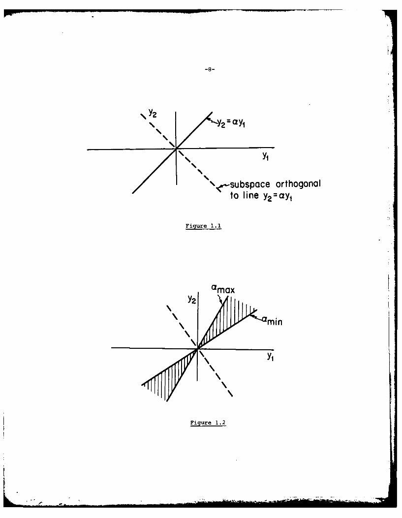
\<'-subspace orthogonal

to line Y2 =ay,

Figure 1. 1

amax 1Y2

Figure 1.2

-9-

optimization problem can be stated in terms of singular values of a parti-

cular matrix. Also, this approach can be viewed as a modification of that

of Chow in that it overcomes the state-dependent nature of the optimum

parity check of Chow. Furthermore, this geometric approach can also be used

to formulate problems which allow one to choose the optimum parity checks

subject not only to performance constraints under normal operation but also

when specific failures occur.

To illustrate the point mentioned at the end of the preceding para-

graph, consider our simple example and suppose that a failure results in

a shift in a. When there are uncertainties in a, this results in a picture

as illustrated in Figure 1.3. Intuitively, we would like to use a parity

check consisting of the orthogonal projection onto a line which makes a

large angle with lines in the unfailed cone and a small angle with lines

in the failed cone. We have obtained a "Neyman-Pearon-like" optimization

formulation for this problem and are presently studying the algorithmic

solution of this problem and the formulation and solution of problems of

distinguishing among a set of possible failures.

y2

Lunfai led

failedl

Figure 1.3

-11-

II. Fault-Tolerant Control Systems

In the preceding progress report (191 we outlined several classes of

discrete-time stochastic control problems that are aimed at providing a

framework for gaining an understanding of fault-tolerant optimal control.

These problems involve a finite-state jump process denoting the operational

status of the system. The system state x evolves according to a linear

stochastic equation parametrized by the finite state process. During the

past year significant progress has been made on the problems described

in [191. These results will be described in detail in the forthcoming

Ph.D. thesis of Mr. H.J. Chizeck [18]. Specifically we have accomplished

the following:

(1) As mentioned in [191, the problem is straightforward when

p is independent of x. However, the qualitative properties

of the solution and of the closed-loop system are suprisingly

complex, and a wide variety of types of behavior can be ob-

tained. We have now derived a series of results and constructed

a set of examples which allow us to understand the possibilities

in more detail.

(2) When the transition probabilities of p depend on x the problem

becomes one of nonlinear stochastic control. This problem

reveals many of the critical properties of fault-tolerant

systems, including hedging and risk-avoidance. In much of our

work in this area we have focussed on the scalar problem where

the dependence of p on x is piecewise-constant. A cursory

glance at this problem indicates that with this formulation

the problem can be solved (via dynamic programming) by ex-

amining a growing (as we go back in time) number of constrained

linear-quadratic problems.

The problem has, however, a significant amount more structure

which we have now characterized. This characterization has

-12-

allowed us to pinpoint the nature of hedging and risk-avoidance

for these systems, to reduce the computational complexity of

the solution by a substantial amount, and to obtain a finite

look-ahead approximation.

(3) We have also completed an investigation of the problem described

in (2) above in the presence of bounded process noise. In

this case the piecewise-quadratic nature of the solution of

(2) is lost in some regions, but the insight from (2) allows

us to obtain an approximation to the cost-to-go which reduces

the problem to one much like that without process noise.

(4) We have also obtained some initial results for the vector version

of the problem of (2). In this case the situation becomes far

more complex, as the regions into which one must divide the

state space at each stage of the algorithm have complex shapes.

Work is continuing on obtaining approximation methods for these

regions much as we did for the costs-to-go in (3).

In addition to these problems we have also made progress in a fault-

tolerant optimal control when we have noisy observations of the state.

Specifically, we have been examining a problem in which a system may switch

from normal operation to a failed condition and where our controller must

decide if and when to switch from a control law optimal for normal opera-

tion (with a criterion specific to normal operation) to one optimal under

failed conditions (perhaps with a different criterion). This is a novel

but exceedingly important sequential decision problem. Specifically,

standard statistical decision problems are aimed at providing a tradeoff

between incorrect decision probabilities and decision delay. For control

problems, these are only indirect performance indicators - e.g. the effect

of a false alarm depends on the performance loss resulting from switching

from the normal control law and the effect of detection delay depends on

the performance loss from using the normal law after the system has failed.

-13-

At this point we have obtained the form of the solution, but much work

remains in developing algorithms and in understanding the nature of the

solution.

I wwmt

-14-

III. Additional Problems in Detection

During the past year we have continued and initiated work along

several directions. Brief descriptions follow:

(l) Decision rules. In the work of Chow described in [8, 17, 191

we describe an algorithm for computing optimum decision rules.

This algorithm was complex computationally, and extensions to

more involved detection problems using this approach are pro-

hibitively complex. The reason for this is that optimum

algorithms attempt to partition the space of possible condi-

tional probability vectors for the given set of hypotheses into

decision regions. The boundaries of these regions are the points

where two decisions yield exactly equal performance. It is our

opinion that most of the computational complexity is due to

this goal of finding the precise boundaries, which involves

obtaining precise statistical predictions of the evolution of

the conditional probabilities under each hypothesis. We have

recently initiated the investigation of suboptimum algorithms

based on approximate descriptions of the evolution of conditional

probabilities. This formulation offers the possibility of

solving far larger problems at reduced computational cost and

with small and perhaps negligible performance loss. These pos-

sibilities remain to be examined.

(2) Complex decision problems. As discussed in [19] there is an

exceedingly large and rich class of problems that involve con-

tinuous processes coupled together with discrete processes whose

transitions represent events in the observed signals or the

underlying systems. The methods we have developed and are

developing for failure detection represent in some sense a

first step in attacking the simplest problems of this type,

i.e., ones in which we must detected isolated and sporadic

events. We have also initiated investigations of problems in

which we wish to detect and identify sequences of events. Such

• • ... I ,

problems are of significance for the reliable control of large

scale systems and, in our opinion, hold the key for solving many

complex signal processing problems. In the preceding progress

report [19] we outlined a generic problem formulation for event-

driven signal generation. During this past year we have built on

this formulation to develop a structure for signal processing

algorithms for event-driven signals. The building blocks for

these algorithms are specialized detection algorithms of the

type one uses for failure detection, and the key problem is one

of developing decision mechanisms based on the outputs of these

simple algorithms. As discussed in (19], the major issue is

one of pruning the tree of possible sequences of events in an

optimum manner. The approximate methods described in (1) above

are potentially of great value for this problem. In addition to

our analytical work, we are also working on several specific

applications. This experience is exceedingly useful in providing

insight into the nature of problems of this type. At this time

we are working on problems of electrocardiogram analysis based

on an event-driven model, efficient edge detection in images,

the detection of objects given remote integral data (which is

of direct application to problems of tomographic tracking of

cold-temperature regions in the ocean), and optimum closed-loop

strategies for searching for objects. The fact that such a wide

variety of problems can be approached essentially from one

unified perspective indicates, we feel, the central importance

of this research effort.

(3) Event-Driven Models for Dynamic Systems. Based on the perspective

in (2), we have initiated a more mathematical aspect of our

research based on the development of simplified event-driven

models for nonlinear systems affected by small amounts of noise

and/or rare events. The motivation for this research is that

the exact analysis of such models or the solutions of problems

of estimation and control for such models may be considerably

more complicated (often these problems are intractable) than

- A - -

-16-

those for simplified models obtained through asymptotic analysis.

As an example, consider the scalar stochastic system described by

the stochastic differential equation

dx(t) = f(x(t))dt + £dw(t) (3.1)

where

-(x-l) x >0

f(x) = (3.2)-(x+l) x < 0

This system is characterized by the property that for time inter-

vals that are small the process behaves like a linear process

near one equilibrium or another, while for long times the

aggregate process sgn(x(t)) converges (as EO) to a Markov

jump process. Consequently, one might expect that estimation

of x(t) based on measurements of the form

dy(t) = x(t)dt + dv(t) (3.3)

might be accomplished based on viewing the process as the

state of an event-driven linear system. More generally, one can

consider analogous models for other nonlinear systems possessing

multiple equilibria and subject to small noise. We already have

some results along the lines indicated for simple examples, and

we are continuing to investigate more general situations. Note

that the estimation algorithms that result are of precisely the

form considered in (2). It is our feeling that this research

direction represents a very promising approach to obtaining a

substantial extension to the class of estimation problems for

which tractable solutions can be found.

-17-

PERSONNEL

During this time period Prof. Alan S. Willsky (principal investigator),

Dr. Stanley B. Gershwin, Prof. B.C. Levy, Prof. R.R. Tenney, Dr. David

Castanon, Prof. Shankar Sastry, and students X.-L. Lou, H.J. Chizeck, P.C.

Doerschuk, D. Rossi, C. Bunks, and M. Coderch have been involved in research

outlined in this status report. Of these people Prof. Willsky, Dr. Gershwin, and

Dr. Castanon have received financial support under this contract, and Mr.

Lon and Mr. Chizeck have been research assistants supported by this contract.

-18-

REFERENCES

(Reference number with asterisks report work performed in part under thiscontract).

*1. C.S. Greene, "An Analysis of the Multiple Model Adaptive ControlAlgorithm," Report ESL-TH-843, Ph.D. Thesis, M.I.T., August 1978.

*2. H. Chizeck and A.S. Willsky, "Towards Fault-Tolerant Optimal Control,"Proc. IEEE Conf. on Decision and Control, San Diego, Calif., Jan. 1979.

*3. C.S. Greene and A.S. Willsky, "Deterministic Stability Analysis of theMultiple Model Adaptive Control Algorithm," Proc. of the 19th IEEEConf. on Dec. and Cont., Albuquerque, N.M., Dec. 1980; extended versionto be submitted to IEEE Trans. Aut. Control.

*4. "Status Report Number One, on the Development of a Methodology for theDetection on System Failures and for the Design of Fault-TolerantControl Systems," Rept. ESL-SR-781, Nov. 15, 1977.

5. R.V. Beard, "Failure Accomodation in Linear Systems Through Self-Reorganization," Rept. MVL-71-1, Man-Vehicle Lab., M.I.T., Cambridge,Mass., Feb. 1971.

6. H.L. Jones, "Failure Detection in Linear Systems," Ph.D. Thesis, Dept.of Aeronautics and Astronautics, M.I.T., Camb., Mass., Sept. 1973.

*7. "Status Report Number Two, on the Development of a Methodology for theDetection of System Failures and for the Design of Fault-Tolerant ControlSystems," Rept. LIDS-SR-873, Dec. 27, 1978.

*8. E.Y. Chow, "A Failure Detection System Design Methdology," Ph.D. Thesis,Dept. of Elec. Eng. and Comp. Sci., M.I.T., Nov. 1980.

9. R.B. Washburn, "The Optimal Sampling Theorem for Partially Ordered TimeProcesses and Multiparameter Stochastic Calculus," Ph.D. Thesis, Dept.of Mathematics, M.I.T., Feb. 1979.

*10. A.S. Willsky, "Failure Detection in Dynamic Systems," paper for AGARDLecture Series NO. 109 on Fault Tolerance Design and Redundancy-Manage-ment Techniques," Athens, Rome and London, October 1980.

*11. "Status Report Number Three, On the Development of a Methodology forthe Detection of System Failures and for the Design of Fault-TolerantControl Systems," Oct. 25, 1979.

12. B.R. Walker, "A Semi-Markov Approach to Quantifying the Performance ofFault-Tolerant Systems," Ph.D. Dissertation, M.I.T., Dept. of Aero.and Astro., Cambridge, Mass., July 1980.

-19-

*13. H.R. Shomber, "An Extended Analysis of the Multiple Model Adaptive

Control Algorithm" S.M. Dissertation, M.I.T., Dept. of Elec. Eng. andComp. Sci., also L.I.D.S. Rept. LIDS-TH-973, Feb. 1980.

*14. D.A. Castanon, H.J. Chizeck, and A.S. Willsky, "Discrete-Time Control

of Hybrid Systems," Proc. 1980 JACC, Aug. 1980, San Francisco.

*15. H.J. Chizeck and A.S. Willsky, "Jump-Linear Quadratic Problems with

State-Independent Rater," Rept. No. LIDS-R-1053, M.I.T., Laboratoryfor Information and Decision Systems, Oct. 1980.

*16. E.Y. Chow and A.S. Willsky, "Issues in the Development of a GeneralDesign Algorithm forr Reliable Failure Detection," Proc. 19th IEEEConf. on Dec. and Control, Albuquerque, New Mexico, December 1980;extended version to be submitted for review for publication.

*17. E.Y. Chow and A.S. Willsky, "Sequential Decision Rules for Failure

Detection," Proc. 1981 JACC, June 1981, Charlottesville, Virginia.

*18. H.J. Chizeck, "Fault-Tolerant Optimal Control", Ph.D. Thesis, Dept.of Elec. Eng. and Comp. Sci., M.I.T., tobe completed in Nov. 1981.

*19. "Status Report Number Four, On the Development of a Methodology forthe Detection of System Failures and for the Design of Fault-TolerantControl Systems," Oct. 1980.

*20. X.-L. Lou, "Robust Failure Detection," S.M. Thesis proposal, Dept. ofElec. Eng. and Comp. Sci., M.I.T., to be completed in Nov. 1981.

-20-

APPENDIX A

Copy of the report on Prof. Alan S. IWillskcy's visit to the People's Republicof China and Japan.

I; I

Massachusetts Institute of TechnologyLaboratory for Information and Decision Systems

Cambridge, MA 02139

REPORT ON TRAVEL TO THE PEOPLE'S REPUBLICOF CHINA AND JAPAN

Supported in part by Contract ONR/N00014-77-C-0224

September 21, 1981

Prepared by: Alan S. Willsky

Submitted to: Dr. Charles HollandMathematics Program (Code 432)

Office of Naval Research800 North Quincy BoulevardArlington, Virginia 22217

-2-

This report summarizes the trip of Prof. Alan S. Willsky to the

People's Republic of China and Japan. The primary purposes of this trip

were to participate in the Bilateral Seminar on Control Systems held in

Shanghai, China and the Seventh Triennial World Congress (held in Kyoto,

Japan) of the International Federation of Automatic Control. The following

is the itinerary followed by Prof. Willsky:

August 9-12 Shanghai, China

August 13-16 Xian, China

August 16-19 Beijing, China

August 19-22 Tokyo, Japan

August 22-29 Kyoto, Japan

Prof. Willsky served as technical program chairman for the meeting

in Shanghai and as one of the organizers of the activities of the

official IEEE Control Systems Society delegation during the entire visit

to China. In addition, Prof. Willsky was one of three plenary speakers

during the Bilateral Seminar. The subject of his talk was an introduction

to and survey of methods for the detection of abrupt changes in signals

and systems. Prof. Willsky's research in this field has been and is

presently supported in part by ONR.

The basic purpose of the visit by the IEEE delegation was to establish

ties between the Control Systems Society and the Chinese Association of

Automation and to provide an opportunity for discussion among researchers

from both organizations. To achieve these objectives, the delegation

organizers structured the visit to allow for ample opportunity for dis-

cussion and for members of the IEEE delegation to gain knowledge and under-

standing about China, the Chinese people, and research in China. In addition

-3-

to the 3-day meeting in Shanghai, there were also visits to Xian and Beijing.

Cultural, social, and technical activities were organized in both of these

cities. In Xian the delegation visited Xian Jiaotong University, and

Prof. Willsky was involved in a discussion of implementation issues for

digital control systems. Also involved in this discussion was Dr. Stuart L.

Brodsky of ONR. In Beijing a technical interchange was held at The

Great Hall of the People.

Overall the visit to China was exceedingly worthwhile. The meeting

in Shanghai was a significant success, and the contacts made there will

allow for continued interaction. In particular, a number of Chinese re-

searchers expressed great interest in Prof. Willsky's lecture and provided

him with information and publications concerning research on failure

detection and adaptive control in China. The visit to Xian Jiaotong

University was also valuable, as it provided the opportunity to see one

of China's leading and fastest growing technical universities. Beyond

these specific scheduled events the many informal, unscheduled discussions

at banquets provided further information about research at institutions

that were not visited.

The other major portion of this trip was the IFAC World Congress,

the largest (approximately 1500 attendees) meeting of researchers in auto-

matic control. In addition to presenting a paper on implementation issues

in digital control and attending various technical sessions, Prof. Willsky

also had the opportunity to discuss research topics with researchers from

many countries. In particular, Prof. Willsky engaged in numerous discussions

on problems of abrupt changes, failure detection and fault-tolerant control.

Prof. Willsky spoke with Prof. K. Astrom of Sweden, Prof. L. Ljung of Sweden,

-4-

Dr. F. Pau of France, Prof. V. Utkin of the Soviet Union, and Prof. A. Halme

of Finland, among others. These discussions were of great value in updating

Prof. Willsky's knowledge of related research around the world. In addition,

Prof. Willsky also was able to learn much about the status and direction of

robotics research in Japan. As this represents an important and promising

direction for future research, the opportunity provided by this visit to

Jpan was a significant one.

I

APPENDIX B

Copy of the paper

Sequential Decision Rules for Failure Detection

by

Edward Y. ChowAlan S. Willsky

L7

July, 1981 LD--l

SEQUENTIAL DEC:STON RULES FOR FAILUaE DEEZC71ON-

Edward Y. Chow, Schlumberger-Doll ResearchRidgefield, Connecticut 06877

A.lan S. illsky, Laboratory for Information and Decision Systems,Massachusetts institute of Technology

Cambridge, MLssachuseccs 02139

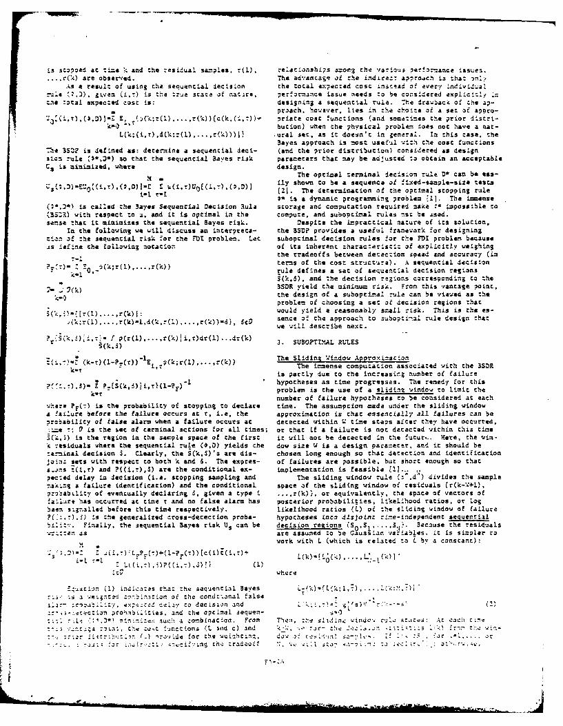
Abstract

The formulation of the decision making of a failure detectionprocess as a Bayes sequential decision problem (3SDP) providesa simple concepcualization of the decision rule design problem.As the optimal Bayes rule is not computable, a methodology chatis based on the Baysian approach and aimed at a reduced. compuca-tilonal requirement is developed for designing suboptimal rules.A numerical algorithm is constructed to facilitate the design andperformance evaluation of these suboptimal rules. The result ofapplying this design methodology to an example shows Chat chisapproach is a useful one.

This work was supported in part by the Office of Naval Research under ContractNo. N00014-77-C-0224 and in pare by NASA Ames Research Canter under Grant ""L-22-O09-24.

1. INTRODUCTION 2. THE 3AYESTAN APPROACH

The failure detection and identification (FDI) The BSDP formulacion of the FDI problem consistsprocess involves monitoring the sensor measurements of six elements:or processed measurements known as the residual (11 1) 0: the set of states of nature or failurefor changes from its normal (no-fail) behavipr. Re- hypotheses. An element i of e may denote a singlesidual samples are observed in sequence. If a failure type i failure of size v occurring at time r(9-is judged to have occurred and sufficient information (i,r,Y)) or the occurrence of a set of failures (pos-(from the residual) has been gathered, the monitoring sibly simultaneously), i.e. -((i, 1 ,). (in,Tprocess is stopped. Then, based on the past obser- V,)'. Due to the infrequent nature of failure, wevacions of residual, an identification of the failure will focus on the case of a single failure.is made. If no failure has occurred, or if the in- In many applications it suffices Co Just identifyformation gathered is insufficient, monitoring is not the failure type without estimating the failure size.interrupted so that further residual samples may be Moreover, it is often true that a detection systemobserved. The decision to interrupt the residual- based on (i,r,-) ftr some appropriate - can also de-

zonitoring to make a failure identification is based tect and identify the type of the failure (i,?,u) foron a compromise between the speed and accuracy of the u>1. Thus, we may use (i,r,V) to represent (i,:).decection, and the failure identification reflecca In the aircraft sensor FD1 problem [31, for instance,the design tradeoff among The errors in failure clas- excellent results were obtained using this approach.3ification. Such a decision mechanism belongs to the Now we have the discrete nature setextensively studied class of sequential tests or se-quential decision rules. 3n this paper, we will em- 3 - ((i,r), i-.......t-,2.oloy the 3ayesian Approach (21 co design decisionrules for FDI systems. where we assume there are X different failure types

In Section 2, we will describe the 3ayes formu- of interest.

lation of the FDI decision problem. Although the 2) v: the prior probabilicy mass function (?MF)optimal rule is generally noc computable, the struc- over the nature set 3. This PMF represents the acure of the Bayesian approach can be used to derive priori information concerning the failure, i.e. now

practical suboptimal rules. We will discuss the de- likely it is for each type of failure to occur, andsi3n of suboptimal rules based on the Bayes formula- when is a failure likel 7 Co occur. Because this in-:ion in Section 3. In Section 4, we will report our formation may not be available or accurrace in someexoerenee ith this approach to designing decision cases, the need to specify u is a drawback of therules through a numerical evample and simulation. 3ayes approach for such -ases. Nevertheless, we will

see that it can be regarded ai a parameter in the de-sign of a Sayes rule.

tn general, u may ie arbitrary. Hera, we ajs!-ethe underlying failure ,rocess ins t'o oroper:s:i) the M failures of D are indcpcn,..n of one inocner,and I) the occurrence or each fa 'ure it s IBernoulli process with -,ceis0 :. 'r - JBernoulti oroces (c2r %' ? SI ?o on i )rrc-

:na inysL onpa.5nci:

-A-2A

describes a large class of failures (such as sensor that the residual is affected by the failure in afailures) while providing a simple approximacion for causal nanner, its zond i:onal density has the prop-the others. !t is straighcforward to show that erty

(i,)' (i)o(l-o) - i-l,...,M, --3,Z ... p(r(l),..r(k)i,1)'p(r(l) ... r(k)Y(0,-))

where l.k

M where (0,-) is used to denQte the no-fail condi:ion.3-1 - a (1-oj) For the design of suboptimal rules, we will assume

J-1 that the residual is an independent Caussian sequence-. - with V(-. matrix) as the time-independent covariance

(i)'Oi(l-o) [ oj(l-o)- - function and gi(k-T) as the mean given that the fail-i- ure (i.T) has occurred. with the covariance assumed

to be the same for all failures, the mean functionThe parameter P may be regarded as the parameter of g(k-T). characterizes the effect of the failurethe combined (Sernoulli) failure process - the oc- (1,T), and it is henceforth called the signature ofcurrencp of the first failure; o(i)can be interpreted (i,r) (with g, (k-r)-O. for 1-O, or Trk). We haveas the mariinal probability that the first failure chosen to study this type of residuals because itsis of type i. Note that the present choice of u in- special structure facilitates the development of in-dicates the arrival of the first failure is memory- sights into the design of decision rules. Moreover,less. This property is useful in obtaining time- the Gaussian assumption is reasonable in many problemsinvariant suboptimal decision rules, and has met jith success in a wide variety of appli-

3) D(k): the discrete set of terminal actions cations, e.g., (3] [4]. (It should be noted that the(failure identifications) available to the decision use of more general probability densities for themaker when the residual-monitoring is stopped at time residual will not add any conceptual difficulty.)k. An element 6 of 9(k)may denote the pair (j,t), 6) c(k,(i,:)): the delay cost function havingi.e. declaration of a type j failure to have occurred the properties:

at time t. Alternatively. 6 may represent an iden-tification of the i-ch failure type without regard r c(i,k-:) ' 0 T<kfor :he failure time, or it may signify the presence c(k,(i, )) -of a failure without specification of its type or 0- r'ktime, i.e. simply an alarm. Since the purpose of FDIis to detect and identify failures that have occurred c(i,k,-T)>c(i,k 2-t) k.>k,>TO(k) should only contain identifications that either -

specify failure times at/before k, or do not specify After a failure has occurred at T, there is a penaltyany failure time. As a result, the number of ter- for delaying the terminal decision until mime k>-minal decisions specifying failures times grows with with the penalty an increasing function of the delayk while the number of decisions not specifying any (k-T). In the absence of a failure, no penalt isrime will remain the same. in addition, D(k) does imposed on the sampling.' in this study we will con-not include the declaration of no failure, since the sider a delay cost function that is linear in theresidual-monitoring is stopped only when a failure delay, i.e. c(i,k-)-c(i)(k-T), where c(i) is a posi-appears to have occurred. tive function of the failure type i, and may be used

4) L(k;9,5): the terminal decision cost func- to provide different delay penalties for differentzion at time k. L(k;i,d) denotes the penalty for types of failures.deciding 6c0(k) at time k when the true state of A sequential decision rule naturally consists ofnature is it(i,). I is assumed to be bounded and two parts: a stopping rule (or sampling plan) and anon-negative and have the structure: terminal decision rule. The stopping rule, denoted

by €(0(0),0(l;r(1)) ... :(k~r(l)...,rk))...... is ai.()i),6) Tck, 60(k) sequence of functions of :he observed residual sam-

ples, with 0(k~r(l). r(k))-, or 0. WhenL_ Trk 60(k) O(k;r(l),....r(k))-l, (0). residual-monitoring or

sampling is stopped (continued) after the k residualWhere L(f,) is the underlying cost function that is samples, r(l)....,r(k) are observed. Alternatively,independent of k; LF denotes the penalty for a false the stopping rule may be defined by another sequencealarm. and it may be generalized to be dependent on of functions '(,(0),&(lr(l)).,(k;r(1).1. it is only meaningful for a terminal action r(k))....), where i(k;r~l). r(k))fl (0) indicates(identificastion) that indicates the correct failure that residual-monitoring has been carried- on up to(and/or time) to receive a lower decision cost than and including time (k-l) and will (not) be stoppedone that indicates the wrong failure (and/or time). after time k when residual samples, r(l).......,k) are'.e further assume that the penalty due to an incor- observed. The functions ' and are related to each-tc- identification of the failure time is only de- other in :he followir.; wn: =:enc on :he error of such an identification. Thatis !or - , ),(k (1 .. . ( ) :!k r l .. . k) •

I-:;

-nc ;'or no -:7c snecificaion with (S):()..he :arr.cn.i ecis :n rule ;s a sequence of

L((i,:I) ', .~) l" *functions. 0-,d0) d(l.-C' .d(.:r(l ,..), raooing r-~.: [':al -22es, r,' i.........') :nto

"'.....-: na rcsidu.al (ohsurva- the ter-inal Action : en '"., The rjncionS5 o,: =1 t h - rtl) ....... (k) fi,:)) d(k'r(,. ,r f r.;:ects the Jec;ion ru v

-:I: e :n-.: r.at zciconnl Aerjitv. A--:mtngo arrive at .- . C.cn :f~2t f2t:Jn) a ::'..c

A-t

is stopped act,-cze11 and the zesidual sampLes, r(I), relscionships amorg the various -3erformance issues.rC*,,) are observied. The ad.'ancage at :he indirez- approach is that on!!.ks a result of using the sequential decision the tocal ex:pected cost insciad of every individ ",1".3 L~). given (,)is the :rue state at nat.:re, performance issue needs to be considered explici:1 -a

the& total expected Cost is: designing a sequential rule. 7he drawback of the 4p-- proach. however. lies in the cho~te or a se: of appro-E, ~k~rl) ,..,~k))c~k(~,t)~ priace cost functions and sotimes the prior distri-

bution) when Che physical proble= does not have a riat-L~k;i~rd~~r~). rk))11 ural set, as it doesn't in general. In this case, Che

3ayes approach is most usef-ul h th cost functionsThe 3SZ? is defined as: determine a sequential deci- (and the prior distribution) considered as designsiom ru.le ($.* so that the sequential Sayes risk parameters that may be adjusced to obtain an acceptableU 3s minimized, where design.

'1 - The optimal terminal decision rule D* can be eas-ily shown to be a sequence of _4I:xed-sanple-size tests

3 uJ.r) 0(i.r)(.D) (2]. The determination of the optimal stopping rulei-L 4* is a dynamic programmning problem 71]. The immense

(*f* is called the 3ayes Sequential Decision Rule storage and computation requ-ired make :* impossible to(3S-I) with respect to -4, and it is optimal in the compute, and suboptimal rules -nsz be .ised.sense that it minimizes the sequential Bayes risk. Despite the impractical nature of its solution,

In the following we will discuss an interprets- the BSDP provides a useful framework for designingz~nof :he sequential risk for the o problem. Lec suboptimal decision. rules for thle FD1 problem because

4s !4_0,ne the .10ll0-i03 notation of its inherent zharacteristcli of explicitly weighing

--I the cradeoffs between detection speed and accuracy (interms of the cost structure) . A sequential decision

0.- rl) r~) rule defines a set of sequential decision regions- S(k.5). and the decision regions correspcnding to the~(k)3SOR yield the minimum risk. From this vantage point,

the design of a subopti-nal rule can be viewed as theproblem of choosin3 a set of decision regions r:,acwould yield a reasonably small risk. This is the es-

~~;rl).~k)-~d~~r~) . r~))6, ~ sence of the approach to suboptinal rule design thatwe will describe next.

' 5k~)iS~!p~~).k)J.3)~)..rk 3. SUBOPTIMAL RUE

E~~- k-)l--r) . (~rl,..1~) The Sliding 'Window Approxirlacionk-t i~rThe icmense computation associated with the 3SDR

is partly due to the increasing number of failure-1 hypotheses as tine progresses. -he remedy for this

I ?rS~k5)1it}(P~)problem is the use of a slidin3 window to limit thek" ubro alrehptee ob cniee tec

where PF(7) is the probability of stopping to declare time. The assumption made under the sliding windowa fail'ure before the failure occurs at T, i.e, the approximation is that essenciall', all failures can beprzbabilicy of ialse alarm when a failure occurs at detected within W time steps aiter the:y have occurred,

-- ! is the &ec of terminal actions for all times; or that if a !ailure is not detected within this timekF,S) is the region in the sample space of the first it will not be detected in the .tutur,.. Hfere, the win-residuals where the sequentilrlc4D)yed h dow size W is a design parameter. and it should be

:erminlal decision S. Clearly, the S~k,S)'s are dis- chosen long enough so that detection and identificationjotn: sets with respect to both k and 6. The expres- of failures are possible, but short enough so thats-ins :(i.r) and ?((iLr),S) are the conditional ex- implementation is feasible [I]..._ptted delay in decision (i.e. stopping sampling and The sliding window rule (,d)divides the sample,.aki=g a failure identification) and the conditional space of the sliding window of residuals Cr(k-,'+l),

proabU cyof eventually declaring i, given a type i .. .. r(k);, or equivalently, the space of vectors offalil~re has occurred at time t and no false alarm has posterior probabilities, likelihood ratios, or logb)en signalled before this time respectively. likelihood ratios (L) of the s ltding window of failure

?(~t)5)is the generalized cross-detection probe- hypotheses into, dIsjoit -Ine-independent seouenrial4 inally. the sequential 3ayes risk Us can be decision r!egions (S SS . s,:. Because the residuals

wr_.izen as are assume to aeCuin .a~les. it is sizvler to'I work with L (which is re lated toL by a constant):

F- L k ; " I -L

whe re

kn l) Lndi~ca:as that t.h,- sequiential Baves L~k.Lkl,........ 7) 1-- .ee-4 :o1.-t'.On of the condtional false

'--- C,!.!. y edza'/ to dccisl,;n and L A; .7) *~S)'

c .n po-~i~ces.and the optimel sequen-s''~ ~: uLc:, -a conbination. From Thie:n :.:e slilin.; -widru . . a a .-At each 171

:ILI- cui r :~-Uncttons (L. and c) and C!V.' ! r~2.:~.: -

f.() '17,./W ;or the wui:hCtn- cL,- or ia.s- . 3 ~-.. Cti:tnS tCn,, tradcf S.~ . tal .-- . -

LCkICSO, fand we will proceed to take one nore obser- theses of dL!ferenc fl~?e :1pes.vation of the residual. The Sayes design problem is The ris. for ising ,) isto deternine a set of regions {S6,S* .S*! that min- N i ( -imites the sequential risk U ({Si}). This represents U (f>*LF' l

= (L..MIS4SO('-l) O.-

a functional minimization problem for which a solution Mis generally very difficult to determine. A simpler + N (alternative to this problem is to constrain the deci- +

sion regions to take on special shapes, iSi(f)}, thatare parameterized by a fl.ied dimensional vector, f, x Pr(L,. (k)cS j, S(k-1)l±,rJof design variables. Then the resulting design pro- 0blem involves the determination of a set of parameter wherevalues f* that minimizes the risk Uw(f). We willfocus our attention on a special sec of parametrized So(k), (k)cS .. .. (W)ES0)sequential decision regions, because they are simple - -and they serve well to illustrate that the Bayesformulation can be exploited, in a systematic fashion, The probabilities required for calculating the riskto obtain simple suboptimal rules that are capable of are given by the recursion:delivering good performance. These decision regionsare: p(L'1_l(k+l)fS0 (k),!,r) -

S(j,Z)-(L(k) :L(kjJ,)>Cf(j,), [U p(L.'-(k) !S0 (k-l),i r)dL,

-,(k)-

€-(jJ)[L(k~ji)-f(jJ,c>-~,)tki -~,) x S pil(k~l) (L_(1-S~-l,,)

( , ) (j ,. ) } (3a) p L'.0l w ) s (k-l) i'r)d i . (k) k>W (5)

S(0,-)-(L(k) : L(k;iJ)1f(iJ), ?r(L.l(k)cS j , S0 (k-1)Wi,T! ?r(So(k-l)i,r}"

- ..... ,...W-l} (3b) f p(Ll(k)!S 0(k-l),id)dL,_I(k), J-0,l .... M (6)

where S(j,:) is the stop-co-declare (j,k-c) region andS(O,-) is the continue region (see Fig. 1). Generally withthe c's may be regarded as design parameters, buthere, £(j,c) is simply taken to be the standard de- Pr(L ,(W)cS ji.:) - I p(L, 1 (') Ii,)dLi(W) (7)

viation of L(k,J,t . "*- Si -To evaluate U'(f), we need to determine the set For M small, numerical integration of (5)-(7) becomes

of probabilities, {Pr(L(k).S(j,t),L(k-l)CS(O,-),..., manageable.L(W)tS(O,-)i,r}, k>W, J-0,1,...,M, Zc'.... ,W-l}, Unfortunately, the transition density,which, indeed, is the goal of many research efforts in p(LW-.(k+l)ILW,.(k),So(k-l),i,r), required in (5) isthe so-called level-crossing problem (5]. Unfortu- difficult to calculate, because LW..l(k) is not anately, useful results (bounds and approximations of Markov process. in order to facilitate computationsuch probabilities) are only available for the scalar of the probabilities, we need to approximate thecase [6],[71,[31. As it stands, each of the proba- transition density. :n approximating the requiredbilities is an integral of a ','W-dimensional Gaussian transition density for L,' :_1(k) we are, in fact, ap-density over the compound region S(O,-)x.. .xS(O,-) proximating the behavior of LW 1 . A simple approx-xS(j,c), which, for large IMW, becomes extremely un- imation is a Gauss-Markov process 4(k) that is definedwieldy and difficult to evaluate, by

The %V-dimensional vector of decision statisticsL(k) corresponds to the MW failure hypotheses, and Z(k+l) - AL(k) +they provide the information necessary for the simul-taneous identification of both failure type and fail- E(&(k)'(t)} * 3B'uO(k-t)ure time. In most applications, such as the aircraftsensor FD1 problem (31 and the detection of freeway where A and B are XxM constant matrices and & is atraffic incidents [41, where the failure time need not white Gaussian sequence with covariance equal to thebe explicitly identified, the failure time resolution (M!xM) matrix 3B'. The reason for choosing this modelpower provided by the full window of decision scatis- is twofold. Firstly, just as I1Wl(k), L(k) iscics is not needed. instead, decision rules that Gaussian. Secondly, Z(k) is Markov so that its tran-e-ploy a few components of L(k) may be used. The sition density can be readily determined. In order todecision rule of this type considered here consists have Z(k) behave like L.1 (k), we set the matrices Aof sequential decision regions that are similar to and 3 and the mean of such that(3) but are only defined in terms of M components ofL) £i(k)E 1 I ._ 1(k)- (8)

5j- ..,_Lk) :Li~:j,W-l)'fj -0_Lk£()=o_!d!ki ) g• SE ,- O ,- :- "9)-

vioj (.a)That is. we have natcei :he -arginal density and the

....... '. (4Ab) ooe-se: cross-cova:ianze ta Li to :hose of ('Cl. k ) L. "k 1 ) f- -' "

It can *e thow that i.-,-n uo'lv specifyr et S4 s the stop-to-declarc-failure-j region and -

0 1s :re zontinue rtgion. Tt should be noted that A -the se of (4) is effective if cross-correlations of -is - hypotheses of the same failure type 3B' - "

sr ii'.! e': :ie are sma1lr :hn chose among hypo-

(~(~i)~. L~1 k~L) -A V(L 4 (k) i using :Ck) w.e have to au;-ent :-d sig-atv-es is:(0) .. g(v-l)]', ..... .~ a proper choice

wnere of v, the rank of Go can be cirease.. : : and 3 will-1i be inver:ible.

7 G.t-0 Non-;indow" Secuenti2l Decision 7-ules

Her e w: Will describe aro:her simple decisionZ -l(k) (k) - Z G_ -1 rule chat has the same decision regions as he 5mph-

t-0 fied sliding window rule (4), but the vector (t) of .4decision statistics is 2bcained differently as follows:0 t >k

k- '- z(k+l) - A z(k) 4 3 r(kl) (13)C (k) " O.C -kO where A is a constant stable M.x1 matrix, and 3 is a

- - |W1 -1 .M= constant matrix of rank H. Unlike the Markov,Oct!/Y G O k k-Wl-r>0 model 1(k) that approxi=ates I-_(k), z(k) is a.k- 0 realizable Markov process driven by the residual. The

advantages of using z as the decision statistic are:C: (gIt),.., 4()1' I) less storage is required, because residual samples

need not be stored as necessary in the sliding windowMoreover, the macrLc A is stable, i.e. the magnitudes scheme, and 2) since z is Markov, the required proba-of all of the eigenvaluas of A are less than unity, bility integrals are of the for= ell) and (12) so thata=i 3 is invertible if G0 or G., , is of rank X. 3e- the same integration algorithn can be direcc-y appliedcause 1 is an artificial process-(i.e. Z is not a co evaluate such integrals. ('t is ?ossible to use adirect function of the residuals r(k)) L(k) can never higher order z, but the added complexity will negatebe implemented for use in (4). the advantages.)

';e may choose other Harkov approximations of In order to form the stazistics z, we need toL C-!(k) chat match che n-step cross-covariance (lem<W) choose the matrices A and 3. %hnen the failure signa-irscea4 of matching the one-step cross-covariance as tures under consideration are constant biases, 5 canin (10). The suitability of a criterion for choosing simply be set to equal Go, and A can be chosen to betae matr1ces A and 5, such as (9) and (10), depends il, where 0<a-l. Then, the term 3r in (13) resemblesdlrec:ly on the failure signatures under consideration g'V-Ir of (2), and it-provides the correlation of thean: may be examined as an issue separate from the residual with the signatures. The time constantiecision rule design problem. Also, a higher order (i/I-*) of Z characterizes the memory span of z justMarl.ov process may be used co approximate LWl. How- as W characterizes that of the sliding window rules.ever, the increase in the computational complexity More generally, if we consider failure signaturesmay negate the benefits of the approximation. that are not constant biases, the choice of A may

:;ow we can approximate the required probabilities still be handled in the same way as in the constant-in :he risk calculation as bias case, but the selection of a 3 matrix is =ore

involved. With some insights into the nature of the,:i (k)zS.,S0 Ck-l)i,rrL(k)s.,S(k-l)Ii,} signatures, a reasonable choice of 3 can often ber , made. To illustrate how this may be accomplished, we

J0',l,... ,M k>W will consider an example with two failure modes and anm-dimensional residual vector. Let

and

?l.:SSo(k.-l)(i,r}1 g1 (k-r) " -

92 Ck-T) - 2 (1-T+l)

Sj That is, g1 is a constant bias, and g2 is a ramo. Ifwhere we have applied the sane decision rule to 1(k) S and S., are not multiples of each other a simpleas .;_l(k). Therefore, Sj and S%(k-L) denote the c oice of B is available:decision regions and the event or continued samplingui to time k for both L,,_ and 1. Assuming 3-iexists, we haveF i?(Z(k+l)ls 0 (k),i,T) - V p(L(k)[S 0 (k-l),i,T)d7(k)r' a

z 0 p( (k~l) = f(k+i)-A(k)fli,r) f 3, and 3,aa,3, wherea 1 and a, are scalar ccn-stanfs, the abo~e hoice of B-has ramz one and is not

((k)IS -), ) k>4 (12) useful for identifying either signa:ure. Suppose webatch process every two residual samples together, i.e.

w.here p( (k) ,r) is the Caussian density of :(k) we use the residual sequencei r = (,,nier :he failure e!,:). Ncw the integrals (L) and k1l,2... Then we can set 3 to be

'±2) rePresent more tractable numerical problems.:n the event :hat 3 is nor invertible, the tran-

dens it" is degenerace and e12) is very difficult ': ;.'A:ate. 'e' ofe:an this probLem can be circum- B S

ven:edi b batch processing the residjals. Thit is, we f' 22ma' consider rho sdfi~a residual sequence: r(k) -

.. ) ,...... '(.01.k) for sore batch Thus, the !itsc and :.'::rou& f : n-.t- .... as :he lc*v : indo:. 'Zn Sad .'L

(and this 3 has rank two). The use of the nodified Pjji)Pp(<i) '-C. t'A. (17)resudual :(k) in this case causes no adverse effect, "since it only lengthens slightly the interval between when the signature of :-e :4aure :odel is a constantc:mes when ter=inal decisions nay be made. A big in- (including the no-fail zase), the reasoning be*indcrease in such intervals i.e., the batch processing (14) holds, and we can iee :hat ?.(ili) jiLl reach aof r(k) .... r(k+v) simultaneously for large v, may steady stare value as : (:he eiaspsed time) increases.however, be undesirable. For problems where the Then, (17) is a valid approxination for a !arge A.signatures vary drastically as a function of the 7or the case where failure signatures are not constants,elapsed time, or the distinguishability among failures the probability of continuing after - time steps (fordepends essentially on these variations, the eWfec- sufficiently large t) may be arbirrarily small. Thetiveness of using z diminishes. In such cases the error introduced by (17) in the risk (and performancesliding window decision rule should provide becter probability) calculation is. consequently, small.performance because of its inherent nature to look Substituting (17) in (16), we getfor a full %indow's worth of signature. 2 2Probability Calculation .f F " )z )i-( +-rL

An algorithm based on 1-dimensional Gaussian i.1quadrature formulas (91 has been developed to compute wherethe probability integrals of (11) and (12) for thecase M-2. (it can be extended to higher dimension 2 = 2 O + 1- 1 (19)t - t bi (t 1 ) +b (.%! ) .1 +(1)with an increase in compucaction.) The details of this i i-I r00quadrature algorithm is described in (1]. Its accu-racy has been assessed via comparison with Monte Carlo P(PAj)- i b (tii)+b (Ali ) ) (20)simulacions (see the numerical example). With this i .0 0 t b( 1 (01i)algorithm we can evaluate the performance probabili-ties and risks associated with the suboptimal decision P is the unconditional false alarm probability, i.e.rules described above. che probability of one false alarm over all time, ti

is the conditional expected delay to decision, givenRisk Calculation that a type i failure has occurred, and P(ij) is the

In t e absence of a failure, the conditional conditional probability of declaring a type j failure,density has beon observed to essentially reach a given chat failure i has occurred. From the assumptionsteady stare at eome finite time T>W.1 Then, for k>T that ?r(S 0 (T)f0,-) 1 and the steady condition (14), itwe ,have can be shown that the-mean time between false alarmcs is

simply (-bG0)- l. Now all the probabilities in (16)-

?r~t(k)cSlIS0 (k-l),0-} - (14) (20) can be computed by using the quadrature algoricnm.Note that the risk expression (18) consists only of

Pr(k)S, - .. ) (-, - finite sums and it can be evaluated with a reasonable

b (k-Tii) k>r>T (15) amount of computational effort. With such an approx----- imation of the sequential risk, we will be able to

consider the problem of determining the decisionThac is. once steady scate is reached, only the rela- regions (the thresholds f) that minimize the risk.rive time (elapsed time) is important. Generally, It should be noted that we could consider choosingfialures occur infrequently, and decision rule with a sec of thresholds that minimize a weighted combine-low false alarm probabilities are employed. Thus, it cion of certain detection probabilities (P(i,j)), theis reasonalbe to assume 1) o-1 ((1-o)T= 1), and 2) expected detection delay (Ei), and the mean time be-?r(S0(T)l0,-} - I. The sequential risk associated tween false alarms (( - b0 )"I). Although such anwith (4) for M-2 can be approximated hy objective function will not result in a Bayesian de-

sign in general, it is a valid design criterion that(f)PL.+(-2.) m o(i)l c+L(ij)]b.(rli)] may be useful for some application.

s F r F i. j- C0 (16) Risk Minimi:ationwhere The risk minimizazion problem has two features

that deserve special attention. Firstly, the sequen-F (-(l-o) tail risk is not a simple function of the threshold E,F 1-5 (1-0) and the derivative with respect no f is not readily

available. Secondly, calculating the risk is a costl7"exn, we seek to replace the infinite sum over t task. Therefore, the zinimum-seeklng procedure to be

in (16) by the finite sum up to t-4 plus a Lerm ap- used must require few function (risk) evaluations, andproxiating the remainder of the infinite sum. Sup- it must not require derivatives. The sequence-of-pose we have been sampling for a steps since the fail- quadratic-prograns (SQ?) algorithm studied by Winfieldure occurred. Define: (10] has been chosen to solve :his ;roblem, because It

does not need any deri.a:ive infcrmarion and it appears?.,ji) L-.,r S0(c-l),iD. 0,,Z to require fewer .'inct:-n a,:.a. iacions then other well-

know algorichrs [10]. F-rr:er-ore, the SOP is simple.f we stop compu:ing the probabilities after A, we and it has quadratic c:nvor;ence. 7ery b~iefly, the

nay apvroximate algorithm consists of the follcwing. Ac each iteration,a quadratic surface is .::ed to :he risk functionlocally, then :he quadratic -odel is -inirized aver ac~nstraint repion (h-nca :ne nane S i The ris-

n we have not been able to prove function is ea,.'.Iuated at :i3 ni:;>'um and is uod in

such conver:, vnce behavior using elmencary techniques. Ic surftace itcina of ::o txt t:teaion. The de-More advanced function-theoretic mechods nay be neces- tnils of the .icr ci iCP to rzs rinirtztonsar".•

A-2 A

Ts retorted i. ?

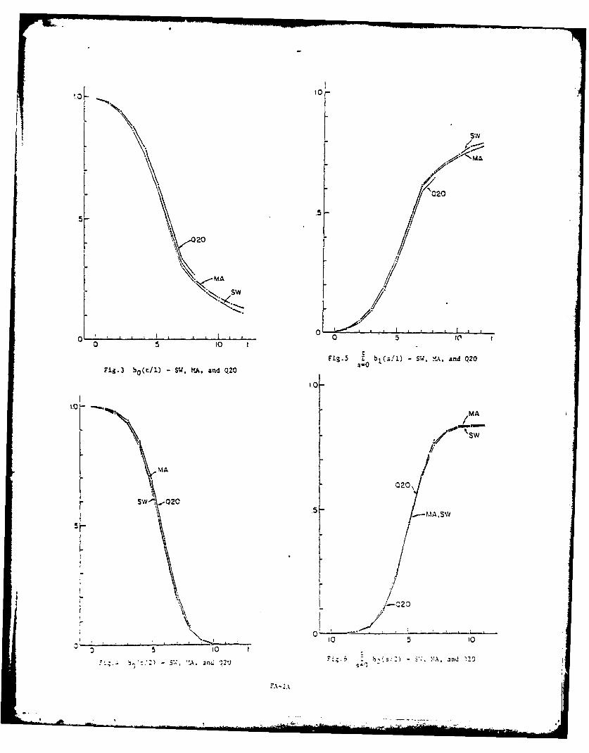
:-ere. we will discuss an applicacion of che sub- cl~c,*locimal rule design =ethodology described above to au=merical example. We wdill consider the detection L(-1r),25(l-o) i-l,2

and idetcification of two possible failure modesCvithout identifying the failure times). We assume p-.0002 T-8 1-8:hat the residual is a 2-dlensional vector, and cherector failure signatures, $1 (t), i-L,2, as functions Table 3. Cast Functions and ?rior ?robabilicv.of the elapsed cime c are shown in Table 1. Thesignature of the first failure zode is simply a con- The results of SW, y.A, and QZO for the thresholdsstart vector. The firsc component of g2 (t) is a con- (8.85, 12.05 are shown in Figs. 2-6 (see (15) for thestart, while the second component is a ramp. We have definition of notations). The quadrature results Q20chosen to examine these two types of signature be- are very close to 4A, indicatla; good accuracy of thenavior (constant bias and ramp) because they are sim- quadrature algorithm. In coaparing SW vich MA., it is3le and describe a large variety of failure signatures evident that the Markov approximation (Mh) slightlythat are commonly seen in practice. For simplicity, under-estimates the false alarm rate of the slidingwe have chosen V, the covariance of r, to be the window rule (5W). However, the response of the Markovisetity =atrLx. approximation to failures is very close to that of the

,e rill design both a simplified sliding window sliding window rule. !n the present exa~ple, L;_1 isrule (that uses L._,) and a rule using the Marko a 7-th order process. while i:s aporoxization isstatistic Z. The parameters associated with the only oi first order. In view of this fact, we can

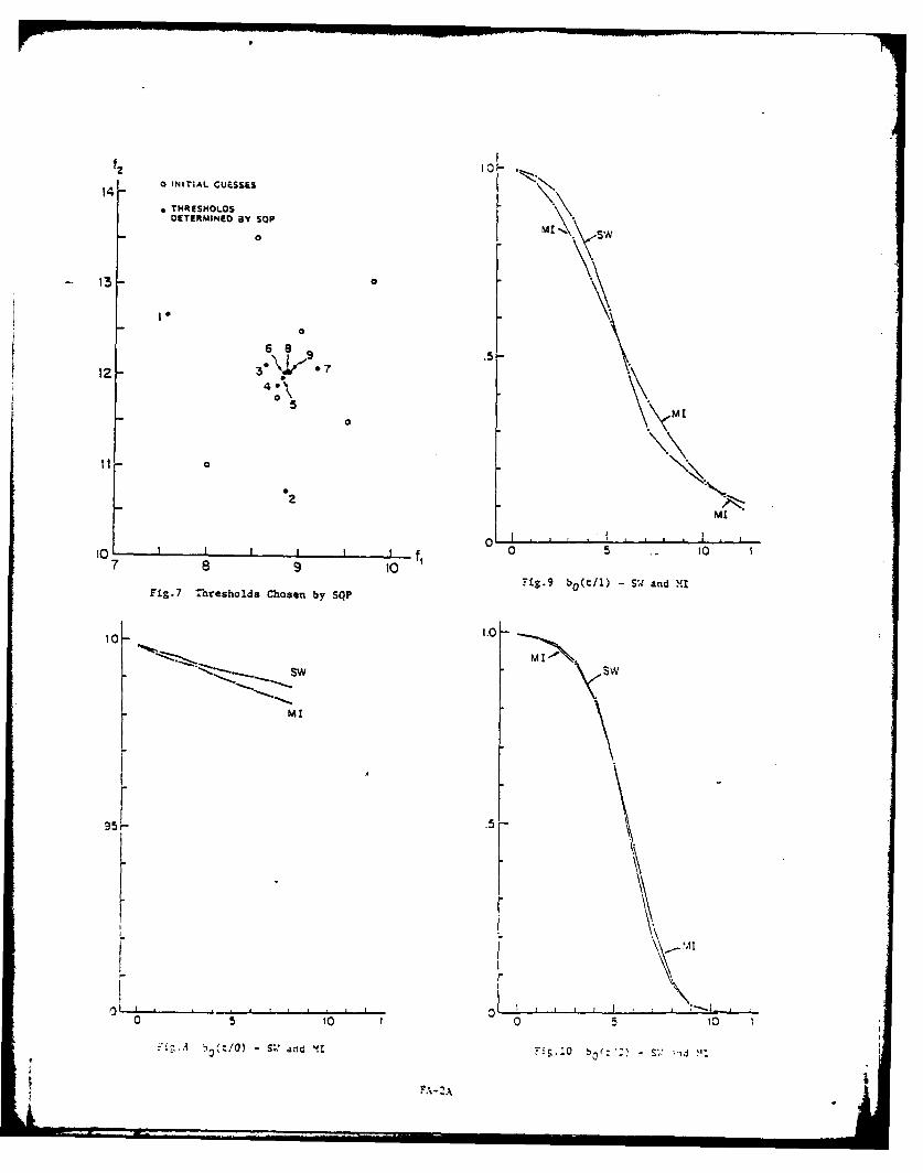
. I, and z are shown in Table 2, and the cost conclude that Z provides a very reasonable and usefulfunctions and the prior probabilities are shown in approximation of 5J-L"Table 3. To facilitate discussions, we will intro- The successive choices of thresholds by SQP forfuce :he folloting terminology. We will refer to a the sliding window rule are plotted in Fig. 7. NoteMante Carlo simulation of the sliding window rule by 'that we have not carried the SQ? algorichm far enoughSW, a simulation of the rule using the Markov scatis- so chat the successive choicas of thresholds are, say,:ic z as Markov implementation (ML), and a simulation within .001 of each ocher. This is because towardsof the nonimplementable decision process using the later iterations the .perfor=a--.:a indices becone rela-aooroximacion Z as Markov approx!mation (MA). (All tively insensitive to s:all changes of the f's. Thissimulations are based on 10,000 trajectones.) The togecher with the fact that w are only conpuctng anrotation Q20 refers to the results of applying the approximate Bayes risk nears chat :Lne scale optimi-quadrature algorithm to the approximation of L.- 1 by zation is not worthwhile. Therefore, with the approx-

imate risk, the SQP is cost efficiently used to locatethe zone where the mini=u= 1!es. That is, the SQPalgorithm is to be terminated -when ic Is evident chat

)g(t) it has converged into a reasonably s-.all region. Then+ .2 J we may choose the thresholds that give the smallest

risk as the approximace solution of the minimization.1 0 In the event that thresholds that yield the small-

V. est risk do not provide the desired detection perfor-L0 lJ mance, the design parameters, L, c, u, and W may be

adjusted and the SQP may be repeated to get a new de-

Table I. Failure signatures. sign. A practical alternative ecrod is to make useof the list of perforcance indices (e.g. ?(i,J)) thatare generated in the risk calculation, and choose a

W 8 pair of thresholds that yields the desired performance.

f826 .058~ The performance of the decision rules using L._116 .08 and z as determined by SQ? are shown in Figs. 3-.Z

•.116 .837 (The thresholds for L,4_1 are (8.35, 12.051 and :hosefor z are (6.29, 11.691.) *e note :hac MI has a

ro 8.5 1 higher false alarm rate than SW. The speed of detec-0 8.5 t.75 tion for the two rules is si=ilar. hile MI has aslightly higher type-I correct detection probability

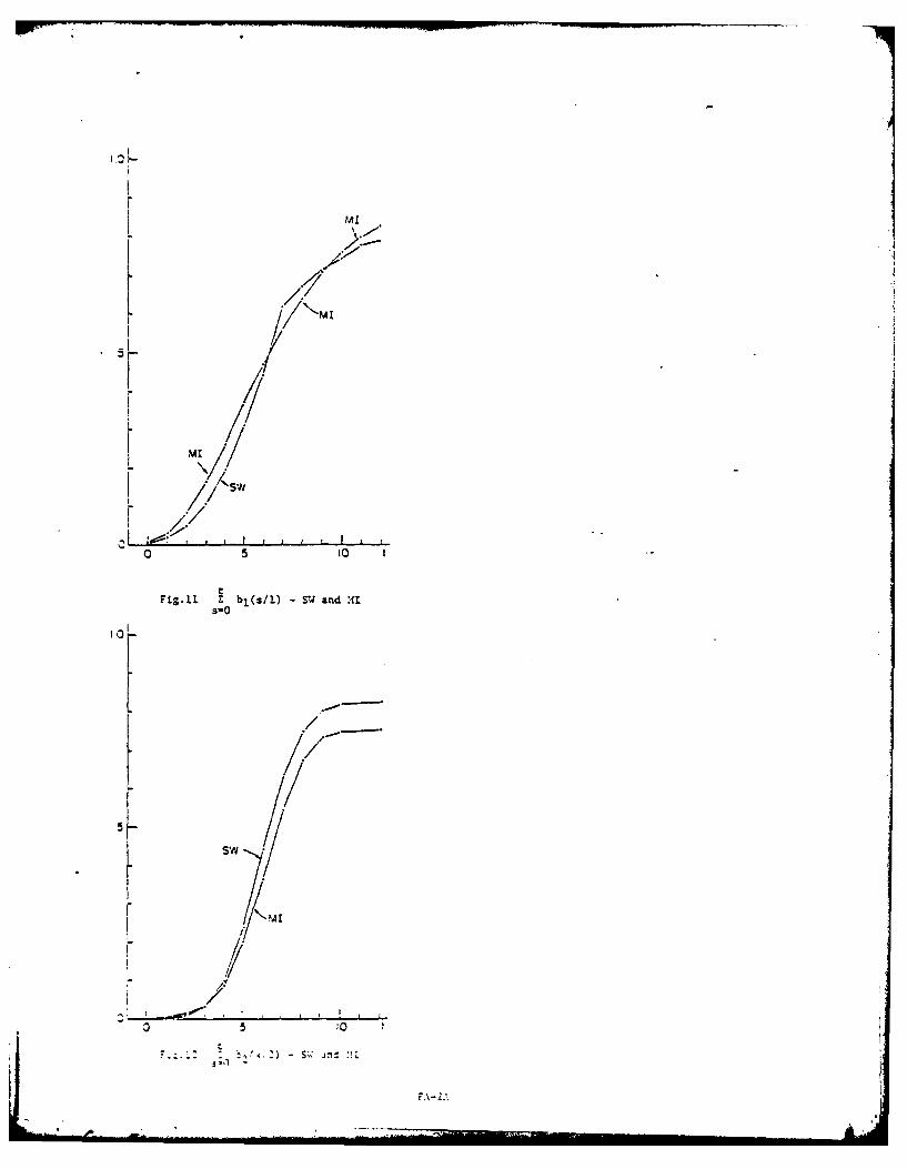
than SW, SW has a consistently hiiher b,(t:2) (type-22.32 2.0L1 correct detection probabilit:..) than 11. 3, raising

33' 12.01 .58J the thresholds of the rule using z approoriatey, wecan decrease the false alsr= race of MI down :o :hac

[.875 0I ., of S*J with an increase in detectlon delay and slightlvA ".improved correct decectian -ro abi t for the :ype-2t0 .85 [. 21 failure (with ramp sienacure) . 7-u3. the S_ dLng

window rule is slight_-: s :: r~or to che rule , sim5.3 5 .401 i [1 r'5 1.501 in the sense that when .bo:6 are 4esignod to vield ,az

S . .1.50 . comvarable false alarm ra:e, the laczer Will ha'.e1.L 4elonger letection delas -in •

c::rrctdectcticn prohability :...-. f:i re In riew

Ta~bl 2. ?ar i-eters for L..-I Z and z. of the fact that a dec s z:n .sle js~r ; * 's 'u.

4iipler :o imple~-n:, :s:5 -- r::" o n z c.As an tL:ernitl:e to tzx 4.. ": .. aw

-. 6 AOL OWL

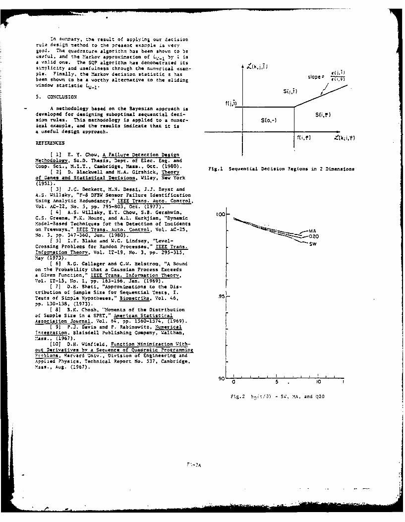
:n su=arv, the result of applying our decisionrule des-g; method to the present example is verygood. The quadrature algorichm has been show to beuseful, and the "arkov approximacion of L-_l by Z isa valid one. The SQP algorithm has decorptrated its £ ,.si=licity and usefulness through the numerical exac- (tpie. Finally, the Markov decision statistic z has slope:been shown to be a worthy alternative to the slidingindow statistic LW_1 . S(1,!

5. CONCLUSION

A methodology based on the Bayesian approach isdeveloped for designing suboptimal sequential deci- su(,)slan rules. This methodology is applied to a numer- S(o,-)ic31 example, and the results indicate that it isa useful design approach. f (i,T) kir

REFERENCES

1] E. Y. Chow, A Failure Detection DesignMethodology, Sc.D. Thesis, Dept. of Elec. Eng. andCamp. Sci., Cambridge, Mass., Oct. (1980). Fig.1 Sequential Decision Regions in 2 Dimensions

C 2] D. Blackwell and M.A. Girshick, Theoryof Games and Statistical Decisions, Wiley, New York(1951).

[ 31 J.C. Deckert, M.N. Desai, J.J. Deysc andA.S. Willsky, "F-8 DFBW Sensor Failure IdentificationUsing Analytic Redundancy," IEEE Trans. Auto. Control,Vol. AC-22, No. 5, pp. 795-803, Oct. (1977).

( 4] A.S. Willsky, E.Y. Chow, S.B. Gershwin, too-C.S. Greene, P.K. Houpc, and A.L. Kurkjian, "DynamicModel-Based Techniques for the Detection of Incidentson Freeways," IEEE Trans. Auto. Control, Vol. AC-25, MNo. 3, pp. 347-360, jun. (1980).

5] I.F. Blake and W.C. Lindsey, "Level- SWCrossing Problems for Randon Processes," IEEE Trans.Infornation Theory, Vol. IT-19, No. 3, pp. 295-315,May (1973).

[ 6] R.G. Gallager and C.W. Helstrom, "A Boundon the Probability that a Gaussian Process Exceedsa Given Function," IEEE Trans. Information Theory,Vol. IT-15, No. 1, pp. 163-166, Jan. (1969).

C 7] D.H. Bhati, "Approximations to the Dis-tribucion of Sample Size for Sequential Tests, 1.,ests of Simple Hypotheses," Biometrika, Vol. 46, 95

pp. 130-138, (1973).C 81 3.K. Chosh, "Moments of the Distribution

of Sample Size in a SPRT," American StatisticalAssociation Journal, Vol. 64, pp. 1560-1574, (1969).

C 91 P.J. Davis and P. Rabinowitz, NumericalIntetration, Blaisdell Publishing Company, Waltham,:ass., (1967).

(10] D.H. Winfield, Function Minimization With-out Derivatives by a Seouence of Quadratic ?roeramming?r ble-, Harvard Univ., Division of Engineering andApplied Physics, Technical Report No. 537, Cambridge, FMass., Aug. (1967).

0 5 to

FIg.2 b,:!0) - S ', MA, and Q20

-,-2A

F0

0 5 10

Fi.5 Zb 1 (s!l) - u.~A and Q20Fig.3 b0 (c/l) -SW, MA. and Q20 0

Nt AA

s/s

~020

5*; 2n -2) A, an 2

14- a iiA USF

o NItAL cua.SSiS

14

*THRESHOLDSDETERMINED BY SOP

0 S

13- 0

00

6 5

12 -3" 7

x7 8 9 0

Fi$.9 b (€/ ) - S W and MI.

4-1

t.0 -

MMI

0 , 1

.5 to

7 8 9 0 0 01

Fi- T e o Chosen - sS and MI-

.l

S-0MS MY

0 5 10

t

Fig.11 Z_ b1(s/J.) - S:J and "41

s-a

0

/ --

/

3 ,