Lab Manual for Physics 222 - lightandmatter.com

Lab Manual for Physics 222

Benjamin Crowell and Virginia RoundyFullerton College

www.lightandmatter.com

Copyright (c) 1999-2011 by B. Crowell and V. Roundy. This lab manual is subject to the Open PublicationLicense, opencontent.org.

2

Contents

1 Electricity . . . . . . . . . . . . . . . . . . . . . . . . . . . . . . . . 62 Electrical Resistance . . . . . . . . . . . . . . . . . . . . . . . . . . . . 123 The Loop and Junction Rules . . . . . . . . . . . . . . . . . . . . . . . . . 164 Electric Fields . . . . . . . . . . . . . . . . . . . . . . . . . . . . . . . 185 Magnetism . . . . . . . . . . . . . . . . . . . . . . . . . . . . . . . . 226 The Oscilloscope . . . . . . . . . . . . . . . . . . . . . . . . . . . . . . 267 Electromagnetism . . . . . . . . . . . . . . . . . . . . . . . . . . . . . 308 The Charge to Mass Ratio of the Electron. . . . . . . . . . . . . . . . . . . . . 369 Relativity . . . . . . . . . . . . . . . . . . . . . . . . . . . . . . . . 4010 Energy in Fields . . . . . . . . . . . . . . . . . . . . . . . . . . . . . . 4411 RC Circuits . . . . . . . . . . . . . . . . . . . . . . . . . . . . . . . . 4612 AC Circuits . . . . . . . . . . . . . . . . . . . . . . . . . . . . . . . . 5013 Faraday’s Law . . . . . . . . . . . . . . . . . . . . . . . . . . . . . . . 5214 Polarization . . . . . . . . . . . . . . . . . . . . . . . . . . . . . . . . 56

Appendix 1: Format of Lab Writeups . . . . . . . . . . . . . . . . . . . . . . 60Appendix 2: Basic Error Analysis . . . . . . . . . . . . . . . . . . . . . . . . 62Appendix 3: Propagation of Errors . . . . . . . . . . . . . . . . . . . . . . . 68Appendix 4: Graphing . . . . . . . . . . . . . . . . . . . . . . . . . . . . 70Appendix 5: Finding Power Laws from Data . . . . . . . . . . . . . . . . . . . . 74Appendix 6: Using a Multimeter . . . . . . . . . . . . . . . . . . . . . . . . 76Appendix 7: High Voltage Safety Checklist . . . . . . . . . . . . . . . . . . . . 78Appendix ??: Comment Codes for Lab Writeups . . . . . . . . . . . . . . . . . . 82Appendix 10: The Open Publication License . . . . . . . . . . . . . . . . . . . . 84

Contents 3

4 Contents

Contents 5

1 Electricity

Apparatusscotch taperubber rodheat lampfurbits of paperrods and strips of various materials30-50 cm rods, and angle brackets, for hanging chargedrodspower supply (Thornton), in lab benches . .1/groupmultimeter (PRO-100), in lab benches . . . . 1/groupalligator clipsflashlight bulbsspare fuses for multimeters — Let students replacefuses themselves.

GoalsDetermine the qualitative rules governing elec-trical charge and forces.

Light up a lightbulb, and measure the currentthrough it and the voltage difference across it.

IntroductionNewton’s law of gravity gave a mathematical for-mula for the gravitational force, but his theory alsomade several important non-mathematical statementsabout gravity:

Every mass in the universe attracts every othermass in the universe.

Gravity works the same for earthly objects asfor heavenly bodies.

The force acts at a distance, without any needfor physical contact.

Mass is always positive, and gravity is alwaysattractive, not repulsive.

The last statement is interesting, especially becauseit would be fun and useful to have access to some

negative mass, which would fall up instead of down(like the “upsydaisium” of Rocky and Bullwinklefame).

Although it has never been found, there is no theo-retical reason why a second, negative type of masscan’t exist. Indeed, it is believed that the nuclearforce, which holds quarks together to form protonsand neutrons, involves three qualities analogous tomass. These are facetiously referred to as “red,”“green,” and “blue,” although they have nothing todo with the actual colors. The force between two ofthe same “colors” is repulsive: red repels red, greenrepels green, and blue repels blue. The force be-tween two different “colors” is attractive: red andgreen attract each other, as do green and blue, andred and blue.

When your freshly laundered socks cling together,that is an example of an electrical force. If the grav-itational force involves one type of mass, and thenuclear force involves three colors, how many typesof electrical “stuff” are there? In the days of Ben-jamin Franklin, some scientists thought there weretwo types of electrical “charge” or “fluid,” while oth-ers thought there was only a single type. In the firstpart of this lab, you will try to find out experimen-tally how many types of electrical charge there are.

The unit of charge is the coulomb, C; one coulombis defined as the amount of charge such that if twoobjects, each with a charge of one coulomb, are onemeter apart, the magnitude of the electrical forcebetween them is 9 × 109 N. Practical applicationsof electricity usually involve an electric circuit, inwhich charge is sent around and around in a cir-cle and recycled. Electric current, I, measures howmany coulombs per second flow past a given point; ashorthand for units of C/s is the ampere, A. Voltage,V , measures the electrical potential energy per unitcharge; its units of J/C can be abbreviated as volts,V. Making the analogy between electrical interac-tions and gravitational ones, voltage is like height.Just as water loses gravitational potential energy bygoing over a waterfall, electrically charged particleslose electrical potential energy as they flow througha circuit. The second part of this lab involves build-ing an electric circuit to light up a lightbulb, andmeasuring both the current that flows through thebulb and the voltage difference across it.

6 Lab 1 Electricity

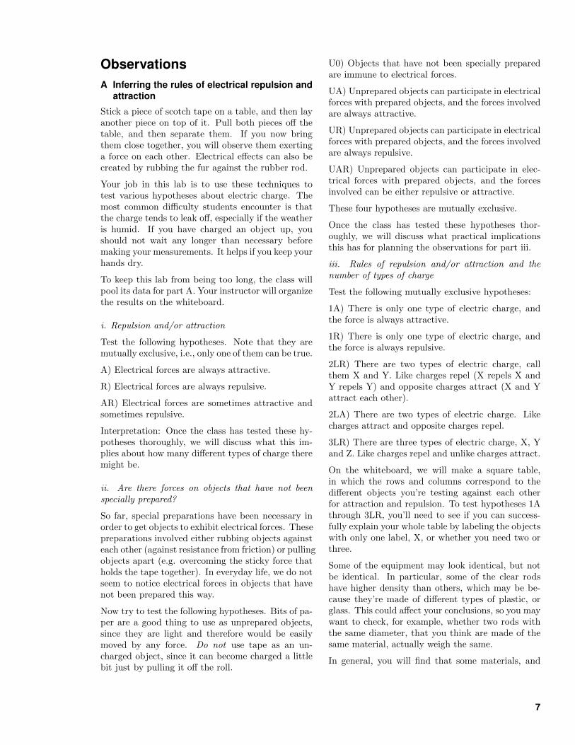
ObservationsA Inferring the rules of electrical repulsion and

attraction

Stick a piece of scotch tape on a table, and then layanother piece on top of it. Pull both pieces off thetable, and then separate them. If you now bringthem close together, you will observe them exertinga force on each other. Electrical effects can also becreated by rubbing the fur against the rubber rod.

Your job in this lab is to use these techniques totest various hypotheses about electric charge. Themost common difficulty students encounter is thatthe charge tends to leak off, especially if the weatheris humid. If you have charged an object up, youshould not wait any longer than necessary beforemaking your measurements. It helps if you keep yourhands dry.

To keep this lab from being too long, the class willpool its data for part A. Your instructor will organizethe results on the whiteboard.

i. Repulsion and/or attraction

Test the following hypotheses. Note that they aremutually exclusive, i.e., only one of them can be true.

A) Electrical forces are always attractive.

R) Electrical forces are always repulsive.

AR) Electrical forces are sometimes attractive andsometimes repulsive.

Interpretation: Once the class has tested these hy-potheses thoroughly, we will discuss what this im-plies about how many different types of charge theremight be.

ii. Are there forces on objects that have not beenspecially prepared?

So far, special preparations have been necessary inorder to get objects to exhibit electrical forces. Thesepreparations involved either rubbing objects againsteach other (against resistance from friction) or pullingobjects apart (e.g. overcoming the sticky force thatholds the tape together). In everyday life, we do notseem to notice electrical forces in objects that havenot been prepared this way.

Now try to test the following hypotheses. Bits of pa-per are a good thing to use as unprepared objects,since they are light and therefore would be easilymoved by any force. Do not use tape as an un-charged object, since it can become charged a littlebit just by pulling it off the roll.

U0) Objects that have not been specially preparedare immune to electrical forces.

UA) Unprepared objects can participate in electricalforces with prepared objects, and the forces involvedare always attractive.

UR) Unprepared objects can participate in electricalforces with prepared objects, and the forces involvedare always repulsive.

UAR) Unprepared objects can participate in elec-trical forces with prepared objects, and the forcesinvolved can be either repulsive or attractive.

These four hypotheses are mutually exclusive.

Once the class has tested these hypotheses thor-oughly, we will discuss what practical implicationsthis has for planning the observations for part iii.

iii. Rules of repulsion and/or attraction and thenumber of types of charge

Test the following mutually exclusive hypotheses:

1A) There is only one type of electric charge, andthe force is always attractive.

1R) There is only one type of electric charge, andthe force is always repulsive.

2LR) There are two types of electric charge, callthem X and Y. Like charges repel (X repels X andY repels Y) and opposite charges attract (X and Yattract each other).

2LA) There are two types of electric charge. Likecharges attract and opposite charges repel.

3LR) There are three types of electric charge, X, Yand Z. Like charges repel and unlike charges attract.

On the whiteboard, we will make a square table,in which the rows and columns correspond to thedifferent objects you’re testing against each otherfor attraction and repulsion. To test hypotheses 1Athrough 3LR, you’ll need to see if you can success-fully explain your whole table by labeling the objectswith only one label, X, or whether you need two orthree.

Some of the equipment may look identical, but notbe identical. In particular, some of the clear rodshave higher density than others, which may be be-cause they’re made of different types of plastic, orglass. This could affect your conclusions, so you maywant to check, for example, whether two rods withthe same diameter, that you think are made of thesame material, actually weigh the same.

In general, you will find that some materials, and

7

some combinations of materials, are more easily charg-ed than others. For example, if you find that themahogony rod rubbed with the weasel fur doesn’tcharge well, then don’t keep using it! The white plas-tic strips tend to work well, so don’t neglect them.

Once we have enough data in the table to reach adefinite conclusion, we will summarize the resultsfrom part A and then discuss the following examplesof incorrect reasoning about this lab.

(1) “The first piece of tape exerted a force on thesecond, but the second didn’t exert one on the first.”(2) “The first piece of tape repelled the second, andthe second attracted the first.”(3) “We observed three types of charge: two thatexert forces, and a third, neutral type.”(4) “The piece of tape that came from the top waspositive, and the bottom was negative.”(5) “One piece of tape had electrons on it, and theother had protons on it.”(6) “We know there were two types of charge, notthree, because we observed two types of interactions,attraction and repulsion.”

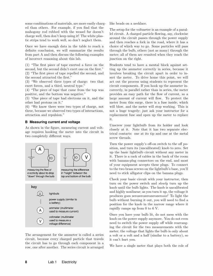
B Measuring current and voltage

As shown in the figure, measuring current and volt-age requires hooking the meter into the circuit intwo completely different ways.

The arrangement for the ammeter is called a seriescircuit, because every charged particle that travelsthe circuit has to go through each component in arow, one after another. The series circuit is arranged

like beads on a necklace.

The setup for the voltmeter is an example of a paral-lel circuit. A charged particle flowing, say, clockwisearound the circuit passes through the power supplyand then reaches a fork in the road, where it has achoice of which way to go. Some particles will passthrough the bulb, others (not as many) through themeter; all of them are reunited when they reach thejunction on the right.

Students tend to have a mental block against set-ting up the ammeter correctly in series, because itinvolves breaking the circuit apart in order to in-sert the meter. To drive home this point, we willact out the process using students to represent thecircuit components. If you hook up the ammeter in-correctly, in parallel rather than in series, the meterprovides an easy path for the flow of current, so alarge amount of current will flow. To protect themeter from this surge, there is a fuse inside, whichwill blow, and the meter will stop working. This isnot a huge tragedy; just ask your instructor for areplacement fuse and open up the meter to replaceit.

Unscrew your lightbulb from its holder and lookclosely at it. Note that it has two separate elec-trical contacts: one at its tip and one at the metalscrew threads.

Turn the power supply’s off-on switch to the off po-sition, and turn its (uncalibrated) knob to zero. Setup the basic lightbulb circuit without any meter init. There is a rack of cables in the back of the roomwith banana-plug connectors on the end, and mostof your equipment accepts these plugs. To connectto the two brass screws on the lightbulb’s base, you’llneed to stick alligator clips on the banana plugs.

Check your basic circuit with your instructor, thenturn on the power switch and slowly turn up theknob until the bulb lights. The knob is uncalibratedand highly nonlinear; as you turn it up, the voltage itproduces goes zerozerozerozerozerosix! To light thebulb without burning it out, you will need to find aposition for the knob in the narrow range where itrapidly ramps up from 0 to 6 V.

Once you have your bulb lit, do not mess with theknob on the power supply anymore. You do not evenneed to switch the power supply off while rearrang-ing the circuit for the two measurements with themeter; the voltage that lights the bulb is only abouta volt or a volt and a half (similar to a battery), soit can’t hurt you.

We have a single meter that plays both the role of

8 Lab 1 Electricity

the voltmeter and the role of the ammeter in this lab.Because it can do both these things, it is referred toas a multimeter. Multimeters are highly standard-ized, and the following instructions are generic onesthat will work with whatever meters you happen tobe using in this lab.

Voltage difference

Two wires connect the meter to the circuit. At theplaces where three wires come together at one point,you can plug a banana plug into the back of anotherbanana plug. At the meter, make one connectionat the “common” socket (“COM”) and the other atthe socket labeled “V” for volts. The common plug iscalled that because it is used for every measurement,not just for voltage.

Many multimeters have more than one scale for mea-suring a given thing. For instance, a meter mayhave a millivolt scale and a volt scale. One is usedfor measuring small voltage differences and the otherfor large ones. You may not be sure in advance whatscale is appropriate, but that’s not a big problem —once everything is hooked up, you can try differentscales and see what’s appropriate. Use the switchor buttons on the front to select one of the voltagescales. By trial and error, find the most precise scalethat doesn’t cause the meter to display an error mes-sage about being overloaded.

Write down your measurement, with the units ofvolts, and stop for a moment to think about whatit is that you’ve measured. Imagine holding yourbreath and trying to make your eyeballs pop outwith the pressure. Intuitively, the voltage differenceis like the pressure difference between the inside andoutside of your body.

What do you think will happen if you unscrew thebulb, leaving an air gap, while the power supplyand the voltmeter are still going? Try it. Inter-pret your observation in terms of the breath-holdingmetaphor.

Current

The procedure for measuring the current differs onlybecause you have to hook the meter up in series andbecause you have to use the “A” (amps) plug on themeter and select a current scale.

In the breath-holding metaphor, the number you’remeasuring now is like the rate at which air flowsthrough your lips as you let it hiss out. Based onthis metaphor, what do you think will happen tothe reading when you unscrew the bulb? Try it.

Discuss with your group and check with your in-

structor:(1) What goes through the wires? Current? Volt-age? Both?(2) Using the breath-holding metaphor, explain whythe voltmeter needs two connections to the circuit,not just one. What about the ammeter?While waiting for your instructor to come aroundand discuss these questions with you, you can go onto the next part of the lab.

Resistance

The ratio of voltage difference to current is calledthe resistance of the bulb, R = ∆V/I. Its units ofvolts per amp can be abbreviated as ohms, Ω (capitalGreek letter omega).

Calculate the resistance of your lightbulb. Resis-tance is the electrical equivalent of kinetic friction.Just as rubbing your hands together heats them up,objects that have electrical resistance produce heatwhen a current is passed through them. This is whythe bulb’s filament gets hot enough to heat up.

When you unscrew the bulb, leaving an air gap, whatis the resistance of the air?

Ohm’s law is a generalization about the electricalproperties of a variety of materials. It states that theresistance is constant, i.e., that when you increasethe voltage difference, the flow of current increasesexactly in proportion. If you have time, test whetherOhm’s law holds for your lightbulb, by cutting thevoltage to half of what you had before and checkingwhether the current drops by the same factor. (Inthis condition, the bulb’s filament doesn’t get hotenough to create enough visible light for your eye tosee, but it does emit infrared light.)

List of materials for static electricity

You don’t have to know anything about what thevarious materials are in order to do this lab, but hereis a list for use by instructors and the lab technician:

• scotch tape (used as two different objects, topand bottom)

• teflon fabric (brown, coarse)

• teflon rods (white, rigid, slippery, skinny)

• PVC pipe

• polyurethane rods (brown, flexible)

• nylon (?) fabric (blue)

• fur

9

Notes For Next Week(1) Next week, when you turn in your writeup forthis lab, you also need to turn in a prelab writeupfor the next lab. The prelab questions are listedat the end of the description of that lab in the labmanual. Never start a lab without understandingthe answers to all the prelab questions; if you turnin partial answers or answers you’re unsure of, dis-cuss the questions with your instructor or with otherstudents to make sure you understand what’s goingon.

(2) You should exchange phone numbers with yourlab partners for general convenience throughout thesemester. You can also get each other’s e-mail ad-dresses by logging in to Spotter and clicking on “e-mail.”

Rules and OrganizationCollection of raw data is work you share with yourlab partners. Once you’re done collecting data, youneed to do your own analysis. E.g., it is not okay fortwo people to turn in the same calculations, or on alab requiring a graph for the whole group to makeone graph and turn in copies.

You’ll do some labs as formal writeups, others asinformal “check-off” labs. As described in the syl-labus, they’re worth different numbers of points, andyou have to do a certain number of each type by theend of the semester.

The format of formal lab writeups is given in ap-pendix 1 on page 60. The raw data section mustbe contained in your bound lab notebook. Typicallypeople word-process the abstract section, and anyother sections that don’t include much math, andstick the printout in the notebook to turn it in. Thecalculations and reasoning section will usually justconsist of hand-written calculations you do in yourlab notebook. You need two lab notebooks, becauseon days when you turn one in, you need your otherone to take raw data in for the next lab. You mayfind it convenient to leave one or both of your note-books in the cupboard at your lab bench wheneveryou don’t need to have them at home to work on;this eliminates the problem of forgetting to bringyour notebook to school.

For a check-off lab, the main thing I’ll pay attentionto is your abstract. The rest of your work for acheck-off lab can be informal, and I may not ask tosee it unless I think there’s a problem after readingyour abstract.

10 Lab 1 Electricity

11

2 Electrical Resistance

ApparatusDC power supply (Thornton) . . . . . . . . . . . . . 1/groupdigital multimeters (Fluke and HP) . . . . . . . 2/groupresistors, various valuesunknown electrical componentsalligator clipsspare fuses for multimeters — Let students replacefuses themselves.

GoalsMeasure curves of voltage versus current forthree objects: your body and two unknownelectrical components.

Determine whether they are ohmic, and if so,determine their resistances.

IntroductionYour nervous system depends on electrical currents,and every day you use many devices based on elec-trical currents without even thinking about it. De-spite its ordinariness, the phenomenon of electriccurrents passing through liquids (e.g., cellular flu-ids) and solids (e.g., copper wires) is a subtle one.For example, we now know that atoms are composedof smaller, subatomic particles called electrons andnuclei, and that the electrons and nuclei are elec-trically charged, i.e., matter is electrical. Thus, wenow have a picture of these electrically charged par-ticles sitting around in matter, ready to create anelectric current by moving in response to an exter-nally applied voltage. Electricity had been used forpractical purposes for a hundred years, however, be-fore the electrical nature of matter was proven at theturn of the 20th century.

Another subtle issue involves Ohm’s law,

I =∆V

R,

where ∆V is the voltage difference applied across anobject (e.g., a wire), and I is the current that flowsin response. A piece of copper wire, for instance,has a constant value of R over a wide range of volt-ages. Such materials are called ohmic. Materialswith non-constant are called non-ohmic. The inter-esting question is why so many materials are ohmic.

Since we know that electrons and nuclei are boundtogether to form atoms, it would be more reasonableto expect that small voltages, creating small electricfields, would be unable to break the electrons andnuclei away from each other, and no current wouldflow at all — only with fairly large voltages shouldthe atoms be split up, allowing current to flow. Thuswe would expect R to be infinite for small voltages,and small for large voltages, which would not beohmic behavior. It is only within the last 50 yearsthat a good explanation has been achieved for thestrange observation that nearly all solids and liquidsare ohmic.

Terminology, Schematics, and Re-sistor Color CodesThe word “resistor” usually implies a specific typeof electrical component, which is a piece of ohmicmaterial with its shape and composition chosen togive a desired value of R. Any piece of an ohmicsubstance, however, has a constant value of R, andtherefore in some sense constitutes a “resistor.” Thewires in a circuit have electrical resistance, but theresistance is usually negligible (a small fraction of anOhm for several centimeters of wire).

The usual symbol for a resistor in an electrical schematicis this , but some recent schematics use

this . The symbol represents a fixed

source of voltage such as a battery, while repre-sents an adjustable voltage source, such as the powersupply you will use in this lab.

In a schematic, the lengths and shapes of the linesrepresenting wires are completely irrelevant, and areusually unrelated to the physical lengths and shapesof the wires. The physical behavior of the circuitdoes not depend on the lengths of the wires (un-less the length is so great that the resistance of thewire becomes non-negligible), and the schematic isnot meant to give any information other than thatneeded to understand the circuit’s behavior. All thatreally matters is what is connected to what.

For instance, the schematics (a) and (b) above arecompletely equivalent, but (c) is different. In thefirst two circuits, current heading out from the bat-

12 Lab 2 Electrical Resistance

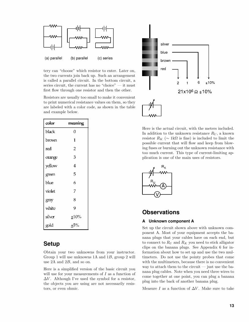
tery can “choose” which resistor to enter. Later on,the two currents join back up. Such an arrangementis called a parallel circuit. In the bottom circuit, aseries circuit, the current has no “choice” — it mustfirst flow through one resistor and then the other.

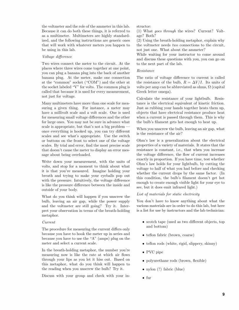
Resistors are usually too small to make it convenientto print numerical resistance values on them, so theyare labeled with a color code, as shown in the tableand example below.

SetupObtain your two unknowns from your instructor.Group 1 will use unknowns 1A and 1B, group 2 willuse 2A and 2B, and so on.

Here is a simplified version of the basic circuit youwill use for your measurements of I as a function of∆V . Although I’ve used the symbol for a resistor,the objects you are using are not necessarily resis-tors, or even ohmic.

Here is the actual circuit, with the meters included.In addition to the unknown resistance RU , a knownresistor RK (∼ 1kΩ is fine) is included to limit thepossible current that will flow and keep from blow-ing fuses or burning out the unknown resistance withtoo much current. This type of current-limiting ap-plication is one of the main uses of resistors.

ObservationsA Unknown component A

Set up the circuit shown above with unknown com-ponent A. Most of your equipment accepts the ba-nana plugs that your cables have on each end, butto connect to RU and RK you need to stick alligatorclips on the banana plugs. See Appendix 6 for in-formation about how to set up and use the two mul-timeters. Do not use the pointy probes that comewith the multimeters, because there is no convenientway to attach them to the circuit — just use the ba-nana plug cables. Note when you need three wires tocome together at one point, you can plug a bananaplug into the back of another banana plug.

Measure I as a function of ∆V . Make sure to take

13

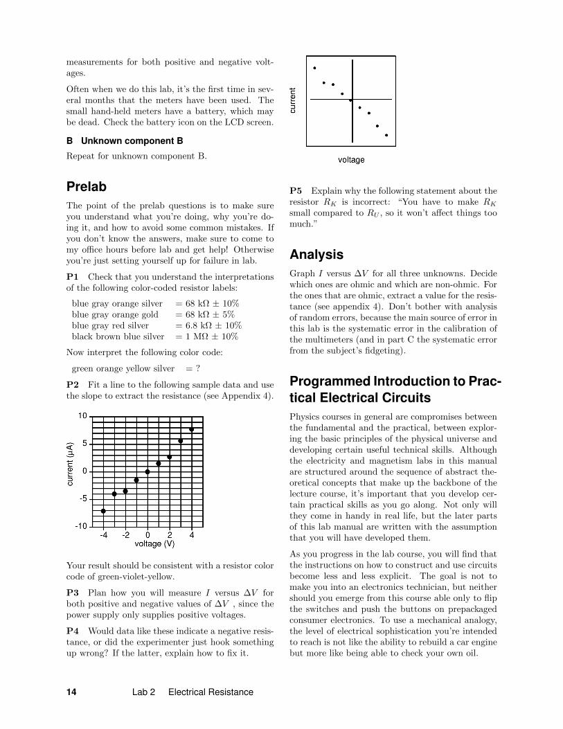
measurements for both positive and negative volt-ages.

Often when we do this lab, it’s the first time in sev-eral months that the meters have been used. Thesmall hand-held meters have a battery, which maybe dead. Check the battery icon on the LCD screen.

B Unknown component B

Repeat for unknown component B.

PrelabThe point of the prelab questions is to make sureyou understand what you’re doing, why you’re do-ing it, and how to avoid some common mistakes. Ifyou don’t know the answers, make sure to come tomy office hours before lab and get help! Otherwiseyou’re just setting yourself up for failure in lab.

P1 Check that you understand the interpretationsof the following color-coded resistor labels:

blue gray orange silver = 68 kΩ ± 10%blue gray orange gold = 68 kΩ ± 5%blue gray red silver = 6.8 kΩ ± 10%black brown blue silver = 1 MΩ ± 10%

Now interpret the following color code:

green orange yellow silver = ?

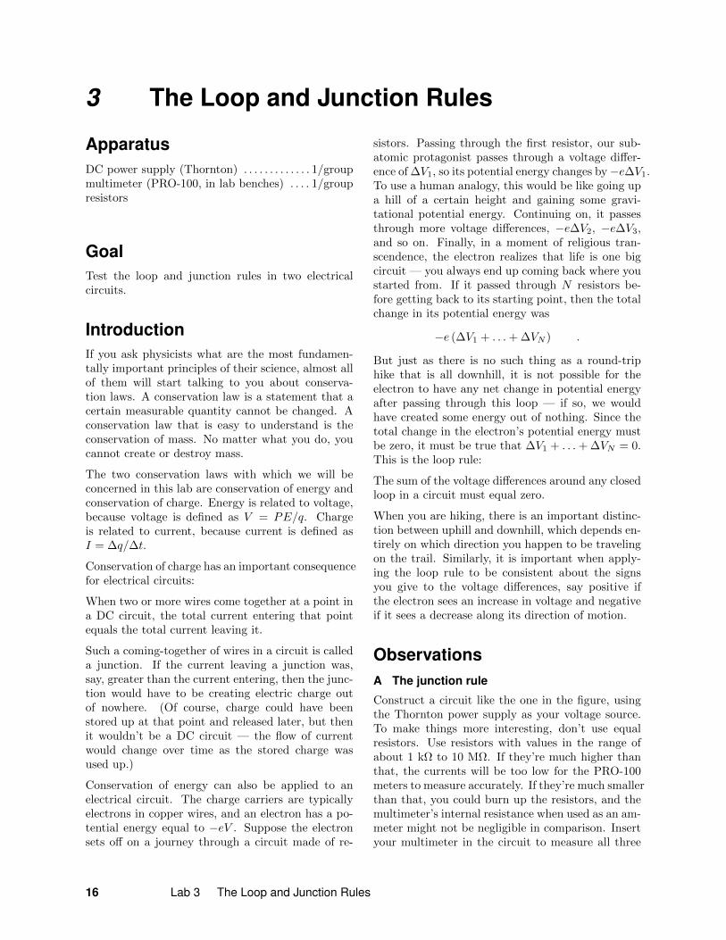
P2 Fit a line to the following sample data and usethe slope to extract the resistance (see Appendix 4).

Your result should be consistent with a resistor colorcode of green-violet-yellow.

P3 Plan how you will measure I versus ∆V forboth positive and negative values of ∆V , since thepower supply only supplies positive voltages.

P4 Would data like these indicate a negative resis-tance, or did the experimenter just hook somethingup wrong? If the latter, explain how to fix it.

P5 Explain why the following statement about theresistor RK is incorrect: “You have to make RKsmall compared to RU , so it won’t affect things toomuch.”

AnalysisGraph I versus ∆V for all three unknowns. Decidewhich ones are ohmic and which are non-ohmic. Forthe ones that are ohmic, extract a value for the resis-tance (see appendix 4). Don’t bother with analysisof random errors, because the main source of error inthis lab is the systematic error in the calibration ofthe multimeters (and in part C the systematic errorfrom the subject’s fidgeting).

Programmed Introduction to Prac-tical Electrical CircuitsPhysics courses in general are compromises betweenthe fundamental and the practical, between explor-ing the basic principles of the physical universe anddeveloping certain useful technical skills. Althoughthe electricity and magnetism labs in this manualare structured around the sequence of abstract the-oretical concepts that make up the backbone of thelecture course, it’s important that you develop cer-tain practical skills as you go along. Not only willthey come in handy in real life, but the later partsof this lab manual are written with the assumptionthat you will have developed them.

As you progress in the lab course, you will find thatthe instructions on how to construct and use circuitsbecome less and less explicit. The goal is not tomake you into an electronics technician, but neithershould you emerge from this course able only to flipthe switches and push the buttons on prepackagedconsumer electronics. To use a mechanical analogy,the level of electrical sophistication you’re intendedto reach is not like the ability to rebuild a car enginebut more like being able to check your own oil.

14 Lab 2 Electrical Resistance

In addition to the physics-based goals stated at thebeginning of this section, you should also be devel-oping the following skills in lab this week:

(1) Be able to translate back and forth between schemat-ics and actual circuits.

(2) Use a multimeter (discussed in Appendix 6),given an explicit schematic showing how to connectit to a circuit.

Further practical skills will be developed in the fol-lowing lab.

15

3 The Loop and Junction Rules

ApparatusDC power supply (Thornton) . . . . . . . . . . . . . 1/groupmultimeter (PRO-100, in lab benches) . . . . 1/groupresistors

GoalTest the loop and junction rules in two electricalcircuits.

IntroductionIf you ask physicists what are the most fundamen-tally important principles of their science, almost allof them will start talking to you about conserva-tion laws. A conservation law is a statement that acertain measurable quantity cannot be changed. Aconservation law that is easy to understand is theconservation of mass. No matter what you do, youcannot create or destroy mass.

The two conservation laws with which we will beconcerned in this lab are conservation of energy andconservation of charge. Energy is related to voltage,because voltage is defined as V = PE/q. Chargeis related to current, because current is defined asI = ∆q/∆t.

Conservation of charge has an important consequencefor electrical circuits:

When two or more wires come together at a point ina DC circuit, the total current entering that pointequals the total current leaving it.

Such a coming-together of wires in a circuit is calleda junction. If the current leaving a junction was,say, greater than the current entering, then the junc-tion would have to be creating electric charge outof nowhere. (Of course, charge could have beenstored up at that point and released later, but thenit wouldn’t be a DC circuit — the flow of currentwould change over time as the stored charge wasused up.)

Conservation of energy can also be applied to anelectrical circuit. The charge carriers are typicallyelectrons in copper wires, and an electron has a po-tential energy equal to −eV . Suppose the electronsets off on a journey through a circuit made of re-

sistors. Passing through the first resistor, our sub-atomic protagonist passes through a voltage differ-ence of ∆V1, so its potential energy changes by−e∆V1.To use a human analogy, this would be like going upa hill of a certain height and gaining some gravi-tational potential energy. Continuing on, it passesthrough more voltage differences, −e∆V2, −e∆V3,and so on. Finally, in a moment of religious tran-scendence, the electron realizes that life is one bigcircuit — you always end up coming back where youstarted from. If it passed through N resistors be-fore getting back to its starting point, then the totalchange in its potential energy was

−e (∆V1 + . . .+ ∆VN ) .

But just as there is no such thing as a round-triphike that is all downhill, it is not possible for theelectron to have any net change in potential energyafter passing through this loop — if so, we wouldhave created some energy out of nothing. Since thetotal change in the electron’s potential energy mustbe zero, it must be true that ∆V1 + . . .+ ∆VN = 0.This is the loop rule:

The sum of the voltage differences around any closedloop in a circuit must equal zero.

When you are hiking, there is an important distinc-tion between uphill and downhill, which depends en-tirely on which direction you happen to be travelingon the trail. Similarly, it is important when apply-ing the loop rule to be consistent about the signsyou give to the voltage differences, say positive ifthe electron sees an increase in voltage and negativeif it sees a decrease along its direction of motion.

ObservationsA The junction rule

Construct a circuit like the one in the figure, usingthe Thornton power supply as your voltage source.To make things more interesting, don’t use equalresistors. Use resistors with values in the range ofabout 1 kΩ to 10 MΩ. If they’re much higher thanthat, the currents will be too low for the PRO-100meters to measure accurately. If they’re much smallerthan that, you could burn up the resistors, and themultimeter’s internal resistance when used as an am-meter might not be negligible in comparison. Insertyour multimeter in the circuit to measure all three

16 Lab 3 The Loop and Junction Rules

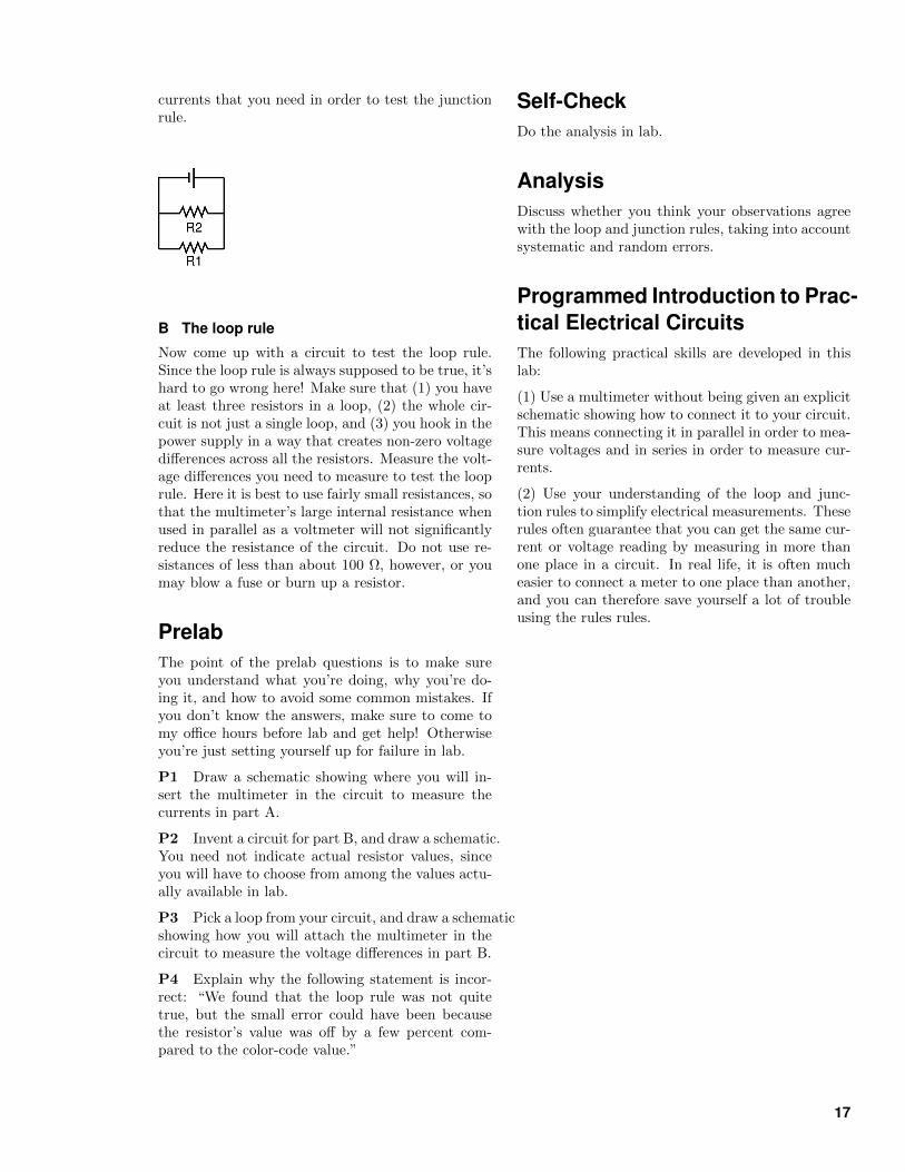
currents that you need in order to test the junctionrule.

B The loop rule

Now come up with a circuit to test the loop rule.Since the loop rule is always supposed to be true, it’shard to go wrong here! Make sure that (1) you haveat least three resistors in a loop, (2) the whole cir-cuit is not just a single loop, and (3) you hook in thepower supply in a way that creates non-zero voltagedifferences across all the resistors. Measure the volt-age differences you need to measure to test the looprule. Here it is best to use fairly small resistances, sothat the multimeter’s large internal resistance whenused in parallel as a voltmeter will not significantlyreduce the resistance of the circuit. Do not use re-sistances of less than about 100 Ω, however, or youmay blow a fuse or burn up a resistor.


P1 Draw a schematic showing where you will in-sert the multimeter in the circuit to measure thecurrents in part A.

P2 Invent a circuit for part B, and draw a schematic.You need not indicate actual resistor values, sinceyou will have to choose from among the values actu-ally available in lab.

P3 Pick a loop from your circuit, and draw a schematicshowing how you will attach the multimeter in thecircuit to measure the voltage differences in part B.

P4 Explain why the following statement is incor-rect: “We found that the loop rule was not quitetrue, but the small error could have been becausethe resistor’s value was off by a few percent com-pared to the color-code value.”

Self-CheckDo the analysis in lab.

AnalysisDiscuss whether you think your observations agreewith the loop and junction rules, taking into accountsystematic and random errors.

Programmed Introduction to Prac-tical Electrical CircuitsThe following practical skills are developed in thislab:

(1) Use a multimeter without being given an explicitschematic showing how to connect it to your circuit.This means connecting it in parallel in order to mea-sure voltages and in series in order to measure cur-rents.

(2) Use your understanding of the loop and junc-tion rules to simplify electrical measurements. Theserules often guarantee that you can get the same cur-rent or voltage reading by measuring in more thanone place in a circuit. In real life, it is often mucheasier to connect a meter to one place than another,and you can therefore save yourself a lot of troubleusing the rules rules.

17

4 Electric Fields

Apparatusboard and U-shaped proberulerDC power supply (Thornton)multimeterscissorsstencils for drawing electrode shapes on paper

GoalsTo be better able to visualize electric fields andunderstand their meaning.

To examine the electric fields around certaincharge distributions.

IntroductionBy definition, the electric field, E, at a particularpoint equals the force on a test charge at that pointdivided by the amount of charge, E = F/q. We canplot the electric field around any charge distributionby placing a test charge at different locations andmaking note of the direction and magnitude of theforce on it. The direction of the electric field atany point P is the same as the direction of the forceon a positive test charge at P. The result would bea page covered with arrows of various lengths anddirections, known as a “sea of arrows” diagram..

In practice, Radio Shack does not sell equipment forpreparing a known test charge and measuring theforce on it, so there is no easy way to measure elec-tric fields. What really is practical to measure at anygiven point is the voltage, V , defined as the elec-trical energy (potential energy) that a test chargewould have at that point, divided by the amountof charge (E/Q). This quantity would have unitsof J/C (Joules per Coulomb), but for conveniencewe normally abbreviate this combination of units asvolts. Just as many mechanical phenomena can bedescribed using either the language of force or thelanguage of energy, it may be equally useful to de-scribe electrical phenomena either by their electricfields or by the voltages involved.

Since it is only ever the difference in potential en-ergy (interaction energy) between two points that

can be defined unambiguously, the same is true forvoltages. Every voltmeter has two probes, and themeter tells you the difference in voltage between thetwo places at which you connect them. Two pointshave a nonzero voltage difference between them ifit takes work (either positive or negative) to movea charge from one place to another. If there is avoltage difference between two points in a conduct-ing substance, charges will move between them justlike water will flow if there is a difference in levels.The charge will always flow in the direction of lowerpotential energy (just like water flows downhill).

All of this can be visualized most easily in termsof maps of constant-voltage curves (also known asequipotentials); you may be familiar with topograph-ical maps, which are very similar. On a topograph-ical map, curves are drawn to connect points hav-ing the same height above sea level. For instance, acone-shaped volcano would be represented by con-centric circles. The outermost circle might connectall the points at an altitude of 500 m, and inside ityou might have concentric circles showing higher lev-els such as 600, 700, 800, and 900 m. Now imaginea similar representation of the voltage surroundingan isolated point charge. There is no “sea level”here, so we might just imagine connecting one probeof the voltmeter to a point within the region tobe mapped, and the other probe to a fixed refer-ence point very far away. The outermost circle onyour map might connect all the points having a volt-age of 0.3 V relative to the distant reference point,and within that would lie a 0.4-V circle, a 0.5-Vcircle, and so on. These curves are referred to asconstant-voltage curves, because they connect pointsof equal voltage. In this lab, you are going to mapout constant-voltage curves, but not just for an iso-lated point charge, which is just a simple examplelike the idealized example of a conical volcano.

You could move a charge along a constant-voltagecurve in either direction without doing any work,because you are not moving it to a place of higherpotential energy. If you do not do any work whenmoving along a constant-voltage curve, there mustnot be a component of electric force along the surface(or you would be doing work). A metal wire is aconstant-voltage curve. We know that electrons in ametal are free to move. If there were a force alongthe wire, electrons would move because of it. In factthe electrons would move until they were distributed

18 Lab 4 Electric Fields

in such a way that there is no longer any force onthem. At that point they would all stay put andthen there would be no force along the wire and itwould be a constant-voltage curve. (More generally,any flat piece of conductor or any three-dimensionalvolume consisting of conducting material will be aconstant-voltage region.)

There are geometrical and numerical relationshipsbetween the electric field and the voltage, so eventhough the voltage is what you’ll measure directlyin this lab, you can also relate your data to electricfields. Since there is not any component of elec-tric force parallel to a constant-voltage curve, elec-tric field lines always pass through constant-voltagecurves at right angles. (Analogously, a stream flow-ing straight downhill will cross the lines on a topo-graphical map at right angles.) Also, if you dividethe work equation (∆energy) = Fd by q, you get(∆energy)/q = (F/q)d, which translates into ∆V =−Ed. (The minus sign is because V goes down whensome other form of energy is released.) This meansthat you can find the electric field strength at a pointP by dividing the voltage difference between the twoconstant-voltage curves on either side of P by thedistance between them. You can see that units ofV/m can be used for the E field as an alternative tothe units of N/C suggested by its definition — theunits are completely equivalent.

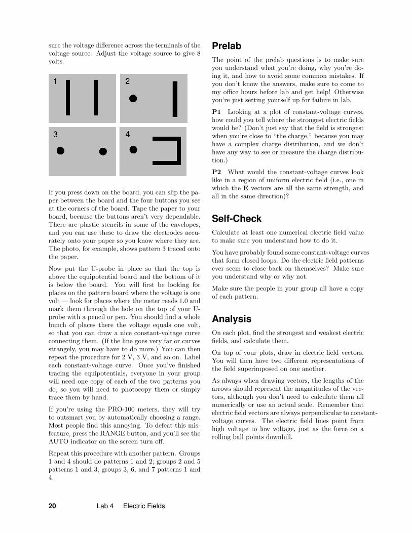
A simplified schematic of the apparatus, being used withpattern 1 on page 20.

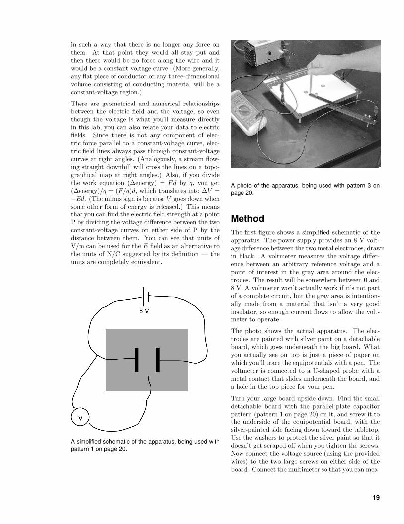
A photo of the apparatus, being used with pattern 3 onpage 20.

MethodThe first figure shows a simplified schematic of theapparatus. The power supply provides an 8 V volt-age difference between the two metal electrodes, drawnin black. A voltmeter measures the voltage differ-ence between an arbitrary reference voltage and apoint of interest in the gray area around the elec-trodes. The result will be somewhere between 0 and8 V. A voltmeter won’t actually work if it’s not partof a complete circuit, but the gray area is intention-ally made from a material that isn’t a very goodinsulator, so enough current flows to allow the volt-meter to operate.

The photo shows the actual apparatus. The elec-trodes are painted with silver paint on a detachableboard, which goes underneath the big board. Whatyou actually see on top is just a piece of paper onwhich you’ll trace the equipotentials with a pen. Thevoltmeter is connected to a U-shaped probe with ametal contact that slides underneath the board, anda hole in the top piece for your pen.

Turn your large board upside down. Find the smalldetachable board with the parallel-plate capacitorpattern (pattern 1 on page 20) on it, and screw it tothe underside of the equipotential board, with thesilver-painted side facing down toward the tabletop.Use the washers to protect the silver paint so that itdoesn’t get scraped off when you tighten the screws.Now connect the voltage source (using the providedwires) to the two large screws on either side of theboard. Connect the multimeter so that you can mea-

19

sure the voltage difference across the terminals of thevoltage source. Adjust the voltage source to give 8volts.

If you press down on the board, you can slip the pa-per between the board and the four buttons you seeat the corners of the board. Tape the paper to yourboard, because the buttons aren’t very dependable.There are plastic stencils in some of the envelopes,and you can use these to draw the electrodes accu-rately onto your paper so you know where they are.The photo, for example, shows pattern 3 traced ontothe paper.

Now put the U-probe in place so that the top isabove the equipotential board and the bottom of itis below the board. You will first be looking forplaces on the pattern board where the voltage is onevolt — look for places where the meter reads 1.0 andmark them through the hole on the top of your U-probe with a pencil or pen. You should find a wholebunch of places there the voltage equals one volt,so that you can draw a nice constant-voltage curveconnecting them. (If the line goes very far or curvesstrangely, you may have to do more.) You can thenrepeat the procedure for 2 V, 3 V, and so on. Labeleach constant-voltage curve. Once you’ve finishedtracing the equipotentials, everyone in your groupwill need one copy of each of the two patterns youdo, so you will need to photocopy them or simplytrace them by hand.

If you’re using the PRO-100 meters, they will tryto outsmart you by automatically choosing a range.Most people find this annoying. To defeat this mis-feature, press the RANGE button, and you’ll see theAUTO indicator on the screen turn off.

Repeat this procedure with another pattern. Groups1 and 4 should do patterns 1 and 2; groups 2 and 5patterns 1 and 3; groups 3, 6, and 7 patterns 1 and4.


P1 Looking at a plot of constant-voltage curves,how could you tell where the strongest electric fieldswould be? (Don’t just say that the field is strongestwhen you’re close to “the charge,” because you mayhave a complex charge distribution, and we don’thave any way to see or measure the charge distribu-tion.)

P2 What would the constant-voltage curves looklike in a region of uniform electric field (i.e., one inwhich the E vectors are all the same strength, andall in the same direction)?

Self-CheckCalculate at least one numerical electric field valueto make sure you understand how to do it.

You have probably found some constant-voltage curvesthat form closed loops. Do the electric field patternsever seem to close back on themselves? Make sureyou understand why or why not.

Make sure the people in your group all have a copyof each pattern.

AnalysisOn each plot, find the strongest and weakest electricfields, and calculate them.

On top of your plots, draw in electric field vectors.You will then have two different representations ofthe field superimposed on one another.

As always when drawing vectors, the lengths of thearrows should represent the magntitudes of the vec-tors, although you don’t need to calculate them allnumerically or use an actual scale. Remember thatelectric field vectors are always perpendicular to constant-voltage curves. The electric field lines point fromhigh voltage to low voltage, just as the force on arolling ball points downhill.

20 Lab 4 Electric Fields

21

5 Magnetism

Apparatusbar magnet (stack of 6 Nd)compassHall effect magnetic field probesLabPro interfaces, DC power supplies, and USB ca-bles2-meter stickHeath solenoids . . . . . . . . . . . . . . . . . . . . . . . . . . .2/groupMastech power supply . . . . . . . . . . . . . . . . . . . . 1/groupwood blocks . . . . . . . . . . . . . . . . . . . . . . . . . . . . . . 2/groupPRO-100 multimeter (in lab bench . . . . . . . .1/groupanother multimeter . . . . . . . . . . . . . . . . . . . . . . . 1/groupD-cell batteries and holdersCenco decade resistor box . . . . . . . . . . . . . . . . 1/group

GoalFind how the magnetic field of a magnet changeswith distance along one of the magnet’s lines of sym-metry.

IntroductionA Variation of Field With Distance: Deflection

of a Magnetic Compass

You can infer the strength of the bar magnet’s fieldat a given point by putting the compass there andseeing how much it is deflected from north.

The task can be simplified quite a bit if you restrictyourself to measuring the magnetic field at pointsalong one of the magnet’s two lines of symmetry,shown in the top figure on the page three pages afterthis one.

If the magnet is flipped across the vertical axis, thenorth and south poles remain just where they were,and the field is unchanged. That means the entiremagnetic field is also unchanged, and the field at apoint such as point b, along the line of symmetry,must therefore point straight up.

If the magnet is flipped across the horizontal axis,then the north and south poles are swapped, and thefield everywhere has to reverse its direction. Thus,the field at points along this axis, e.g., point a, mustpoint straight up or down.

Line up your magnet so it is pointing east-west.

Choose one of the two symmetry axes of your mag-net, and measure the deflection of the compass attwo points along that axis, as shown in the figure atthe end of the lab. As part of your prelab, you willuse vector addition to find an equation for Bm/Be,the magnet’s field in units of the Earth’s, in termsof the deflection angle θ. For your first point, findthe distance r at which the deflection is 70 degrees;this angle is chosen because it’s about as big as itcan be without giving very poor relative precisionin the determination of the magnetic field. For yoursecond data-point, use twice that distance. By whatfactor does the field decrease when you double r?

The lab benches contain iron or steel parts that dis-tort the magnetic field. You can easily observe thissimply by putting a compass on the top of the benchand sliding it around to different places. To workaround this problem, lay a 2-meter stick across thespace between two lab benches, and carry out theexperiment along the line formed by the stick. Evenin the air between the lab benches, the magneticfield due to the building materials in the building issignificant, and this field varies from place to place.Therefore you should move the magnet while keepingthe compass in one place. Then the field from thebuilding becomes a fixed part of the background ex-perienced by the compass, just like the earth’s field.

Note that the measurements are very sensitive to therelative position and orientation of the bar magnetand compass.

Based on your two data-points, form a hypothesisabout the variation of the magnet’s field with dis-tance according to a power law B ∝ rp.

B Variation of Field With Distance: Hall EffectMagnetometer

In this part of the lab, you will test your hypothesisabout the power law relationship B ∝ rp; you willfind out whether the field really does obey such alaw, and if it does, you will determine p accurately.

This part of the lab uses a device called a Hall ef-fect magnetometer for measuring magnetic fields. Itworks by sending an electric current through a sub-stance, and measuring the force exerted on thosemoving charges by the surrounding magnetic field.The probe only measures the component of the mag-netic field vector that is parallel to its own axis. Plugthe probe into CH 1 of the LabPro interface, connect

22 Lab 5 Magnetism

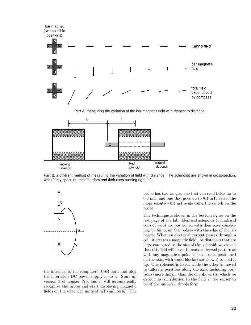
Part A, measuring the variation of the bar magnet’s field with respect to distance.

Part B, a different method of measuring the variation of field with distance. The solenoids are shown in cross-section,with empty space on their interiors and their axes running right-left.

the interface to the computer’s USB port, and plugthe interface’s DC power supply in to it. Start upversion 3 of Logger Pro, and it will automaticallyrecognize the probe and start displaying magneticfields on the screen, in units of mT (millitesla). The

probe has two ranges, one that can read fields up to0.3 mT, and one that goes up to 6.4 mT. Select themore sensitive 0.3 mT scale using the switch on theprobe.

The technique is shown in the bottom figure on thelast page of the lab. Identical solenoids (cylindricalcoils of wire) are positioned with their axes coincid-ing, by lining up their edges with the edge of the labbench. When an electrical current passes through acoil, it creates a magnetic field. At distances that arelarge compared to the size of the solenoid, we expectthat this field will have the same universal pattern aswith any magnetic dipole. The sensor is positionedon the axis, with wood blocks (not shown) to hold itup. One solenoid is fixed, while the other is movedto different positions along the axis, including posi-tions (more distant than the one shown) at which weexpect its contribution to the field at the sensor tobe of the universal dipole form.

23

The key to the high precision of the measurementis that in this configuration, the fields of the twosolenoids can be made to cancel at the position of theprobe. Because of the solenoids’ unequal distancesfrom the probe, this requires unequal currents. Be-cause the fields cancel, the probe can be used on itsmost sensitive and accurate scale; it can also be ze-roed when the circuits are open, so that the effect ofany ambient field is removed. For example, supposethat at a certain distance rm, the current Im throughthe moving coil has to be five times greater than thecurrent If through the fixed coil at the constant dis-tance rf . Then we have determined that the fieldpattern of these coils is such that increasing the dis-tance along the axis from rf to rm causes the fieldto fall off by a factor of five.

It’s a good idea to take data all the way down torm = 0, since this makes it possible to see on agraph where the field does and doesn’t behave like adipole. Note that the distances rf and rm can’t bemeasured directly with good precision.

The Mastech power supply is capable of delivering alarge amount of current, so it can be used to provideIm, which needs to be high when rm is large. Thepower supply has some strange behavior that makesit not work unless you power it up in exactly theright way. It has four knobs, going from left to right:(1) current regulation, (2) over-voltage protection,(3) fine voltage control, (4) coarse voltage control.Before turning the power supply on, turn knobs 1and 2 all the way up, and knobs 3 and 4 all the waydown. Turn the power supply on. Now use knobs 3and 4 to control how much current flows.

At large values of rm, it can be difficult to get apower supply to give a small enough If . Try using abattery, and further reducing the current by placinganother resistance in series with the coil. The Cencodecade resistance boxes can be used for this purpose;they are variable resistors whose resistance can bedialed up as desired using decimal knobs. Use theplugs on the resistance box labeled H and L.

For every current measurement, make sure to usethe most sensitive possible scale on the meter to getas many sig figs as possible. This is why the am-meter built into the Mastech power supply is notuseful here. I found it to be a hassle to measure Imwith an ammeter, because the currents required wereoften quite large, and I kept inadvertently blowingthe fuse on the milliamp scale. For this reason, youmay actually want to measure Vm, the voltage dif-ference across the moving solenoid. Conceptually,magnetic fields are caused by moving charges, cur-

rent is a measure of moving charge, and thereforecurrent is what is relevant here. But if the DC re-sistance of the coil is fixed, the current and voltageare proportional to one another, assuming that thevoltage is measured directly across the coil and theresistance of the banana-plug connections is eithernegligible or constant.

As shown in a lecture demonstration, deactivatingthe electromagnet requires getting rid of the energystored in the magnetic field, and this can be done inmore than one way. If you use your hand to breakthe circuit by pulling out a banana plug, the energyis dissipated in a spark, and a large value of Im isbeing used the result can be an unpleasant shock.To avoid this, deactivate the moving coil by turningdown the knob on the power supply rather than bybreaking the circuit.


P1 In part A, suppose that when the compass is11.0 cm from the magnet, it is 45 degrees away fromnorth. What is the strength of the bar magnet’s fieldat this location in space, in units of the Earth’s field?

P2 Find Bm/Be in terms of the deflection angle θmeasured in part A. As a special case, you shouldbe able to recover your answer to P1.

AnalysisDetermine the variation of the solenoid’s magneticfield with distance. Look for a power-law relation-ship using the log-log graphing technique describedin appendix 5. Does the power law hold for allthe distances you investigated, or only at large dis-tances? No error analysis is required.

24 Lab 5 Magnetism

25

6 The Oscilloscope

Apparatusoscilloscope (Tektronix TDS 1001B) . . . . . . 1/groupmicrophone (RS 33-1067) . . . . . . . . . . . . . for 6 groupsmicrophone (Shure C606) . . . . . . . . . . . . . . for 1 groupPI-9587C sine wave generator . . . . . . . . . . . . .1/groupvarious tuning forks, mounted on wooden boxes

If there’s an equipment conflict with respect to thesine wave generators, the HP200CD sine wave gen-erators can be used instead.

GoalsLearn to use an oscilloscope.

Observe sound waves on an oscilloscope.

IntroductionOne of the main differences you will notice betweenyour second semester of physics and the first is thatmany of the phenomena you will learn about arenot directly accessible to your senses. For example,electric fields, the flow of electrons in wires, and theinner workings of the atom are all invisible. Theoscilloscope is a versatile laboratory instrument thatcan indirectly help you to see what’s going on.

The Oscilloscope

An oscilloscope graphs an electrical signal that variesas a function of time. The graph is drawn from left toright across the screen, being painted in real time asthe input signal varies. In this lab, you will be usingthe signal from a microphone as an input, allowingyou to see sound waves.

The input signal is supplied in the form of a voltage.You are already familiar with the term “voltage”from common speech, but you may not have learnedthe formal definition yet in the lecture course. Volt-age, measured in metric units of volts (V), is definedas the electrical potential energy per unit charge.For instance if 2 nC of charge flows from one ter-minal of a 9-volt battery to the other terminal, thepotential energy consumed equals 18 nJ. To use amechanical analogy, when you blow air out betweenyour lips, the flowing air is like an electrical current,

and the difference in pressure between your mouthand the room is like the difference in voltage. Forthe purposes of this lab, it is not really necessaryfor you to work with the fundamental definition ofvoltage.

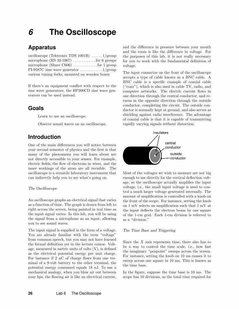
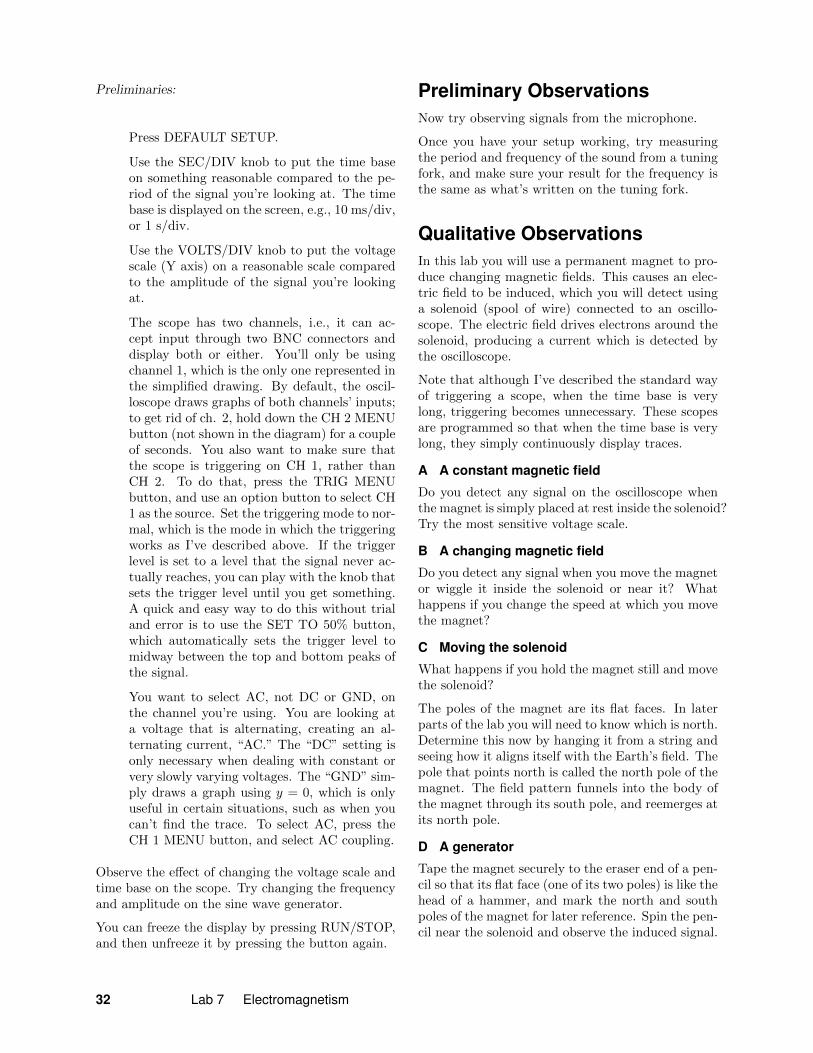
The input connector on the front of the oscilloscopeaccepts a type of cable known as a BNC cable. ABNC cable is a specific example of coaxial cable(“coax”), which is also used in cable TV, radio, andcomputer networks. The electric current flows inone direction through the central conductor, and re-turns in the opposite direction through the outsideconductor, completing the circuit. The outside con-ductor is normally kept at ground, and also serves asshielding against radio interference. The advantageof coaxial cable is that it is capable of transmittingrapidly varying signals without distortion.

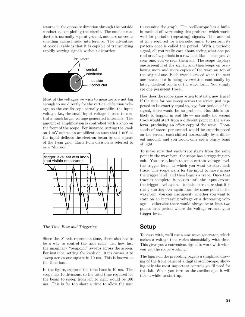
Most of the voltages we wish to measure are not bigenough to use directly for the vertical deflection volt-age, so the oscilloscope actually amplifies the inputvoltage, i.e., the small input voltage is used to con-trol a much larger voltage generated internally. Theamount of amplification is controlled with a knob onthe front of the scope. For instance, setting the knobon 1 mV selects an amplification such that 1 mV atthe input deflects the electron beam by one squareof the 1-cm grid. Each 1-cm division is referred toas a “division.”

The Time Base and Triggering

Since the X axis represents time, there also has tobe a way to control the time scale, i.e., how fastthe imaginary “penpoint” sweeps across the screen.For instance, setting the knob on 10 ms causes it tosweep across one square in 10 ms. This is known asthe time base.

In the figure, suppose the time base is 10 ms. Thescope has 10 divisions, so the total time required for

26 Lab 6 The Oscilloscope

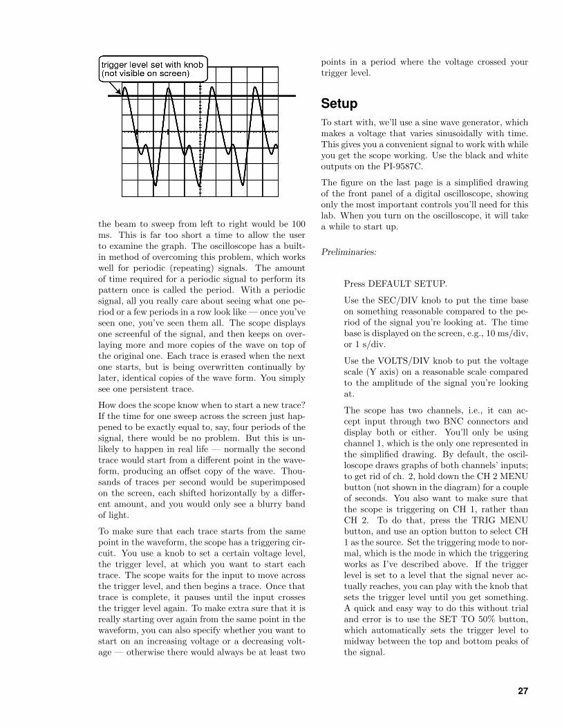
the beam to sweep from left to right would be 100ms. This is far too short a time to allow the userto examine the graph. The oscilloscope has a built-in method of overcoming this problem, which workswell for periodic (repeating) signals. The amountof time required for a periodic signal to perform itspattern once is called the period. With a periodicsignal, all you really care about seeing what one pe-riod or a few periods in a row look like — once you’veseen one, you’ve seen them all. The scope displaysone screenful of the signal, and then keeps on over-laying more and more copies of the wave on top ofthe original one. Each trace is erased when the nextone starts, but is being overwritten continually bylater, identical copies of the wave form. You simplysee one persistent trace.

How does the scope know when to start a new trace?If the time for one sweep across the screen just hap-pened to be exactly equal to, say, four periods of thesignal, there would be no problem. But this is un-likely to happen in real life — normally the secondtrace would start from a different point in the wave-form, producing an offset copy of the wave. Thou-sands of traces per second would be superimposedon the screen, each shifted horizontally by a differ-ent amount, and you would only see a blurry bandof light.

To make sure that each trace starts from the samepoint in the waveform, the scope has a triggering cir-cuit. You use a knob to set a certain voltage level,the trigger level, at which you want to start eachtrace. The scope waits for the input to move acrossthe trigger level, and then begins a trace. Once thattrace is complete, it pauses until the input crossesthe trigger level again. To make extra sure that it isreally starting over again from the same point in thewaveform, you can also specify whether you want tostart on an increasing voltage or a decreasing volt-age — otherwise there would always be at least two

points in a period where the voltage crossed yourtrigger level.

SetupTo start with, we’ll use a sine wave generator, whichmakes a voltage that varies sinusoidally with time.This gives you a convenient signal to work with whileyou get the scope working. Use the black and whiteoutputs on the PI-9587C.

The figure on the last page is a simplified drawingof the front panel of a digital oscilloscope, showingonly the most important controls you’ll need for thislab. When you turn on the oscilloscope, it will takea while to start up.

Preliminaries:

Press DEFAULT SETUP.

Use the SEC/DIV knob to put the time baseon something reasonable compared to the pe-riod of the signal you’re looking at. The timebase is displayed on the screen, e.g., 10 ms/div,or 1 s/div.

Use the VOLTS/DIV knob to put the voltagescale (Y axis) on a reasonable scale comparedto the amplitude of the signal you’re lookingat.

The scope has two channels, i.e., it can ac-cept input through two BNC connectors anddisplay both or either. You’ll only be usingchannel 1, which is the only one represented inthe simplified drawing. By default, the oscil-loscope draws graphs of both channels’ inputs;to get rid of ch. 2, hold down the CH 2 MENUbutton (not shown in the diagram) for a coupleof seconds. You also want to make sure thatthe scope is triggering on CH 1, rather thanCH 2. To do that, press the TRIG MENUbutton, and use an option button to select CH1 as the source. Set the triggering mode to nor-mal, which is the mode in which the triggeringworks as I’ve described above. If the triggerlevel is set to a level that the signal never ac-tually reaches, you can play with the knob thatsets the trigger level until you get something.A quick and easy way to do this without trialand error is to use the SET TO 50% button,which automatically sets the trigger level tomidway between the top and bottom peaks ofthe signal.

27

You want to select AC, not DC or GND, onthe channel you’re using. You are looking ata voltage that is alternating, creating an al-ternating current, “AC.” The “DC” setting isonly necessary when dealing with constant orvery slowly varying voltages. The “GND” sim-ply draws a graph using y = 0, which is onlyuseful in certain situations, such as when youcan’t find the trace. To select AC, press theCH 1 MENU button, and select AC coupling.

Observe the effect of changing the voltage scale andtime base on the scope. Try changing the frequencyand amplitude on the sine wave generator.

You can freeze the display by pressing RUN/STOP,and then unfreeze it by pressing the button again.

Preliminary ObservationsNow try observing signals from the microphone.

Notes for the group that uses the Shure mic: As withthe Radio Shack mics, polarity matters. The tip ofthe phono plug connector is the live connection, andthe part farther back from the tip is the groundedpart. You can connect onto the phono plug withalligator clips.

Once you have your setup working, try measuringthe period and frequency of the sound from a tuningfork, and make sure your result for the frequency isthe same as what’s written on the tuning fork.

ObservationsA Periodic and nonperiodic speech sounds

Try making various speech sounds that you can sus-tain continuously: vowels or certain consonants suchas “sh,” “r,” “f” and so on. Which are periodic andwhich are not?

Note that the names we give to the letters of thealphabet in English are not the same as the speechsounds represented by the letter. For instance, theEnglish name for “f” is “ef,” which contains a vowel,“e,” and a consonant, “f.” We are interested in thebasic speech sounds, not the names of the letters.Also, a single letter is often used in the English writ-ing system to represent two sounds. For example,the word “I” really has two vowels in it, “aaah” plus“eee.”

B Loud and soft

What differentiates a loud “aaah” sound from a softone?

C High and low pitch

Try singing a vowel, and then singing a higher notewith the same vowel. What changes?

D Differences among vowel sounds

What differentiates the different vowel sounds?

E Lowest and highest notes you can sing

What is the lowest frequency you can sing, and whatis the highest?


P1 In the sample oscilloscope trace shown on page31, what is the period of the waveform? What is itsfrequency? The time base is 10 ms.

P2 In the same example, again assume the timebase is 10 ms/division. The voltage scale is 2 mV/div-ision. Assume the zero voltage level is at the middleof the vertical scale. (The whole graph can actuallybe shifted up and down using a knob called “posi-tion.”) What is the trigger level currently set to? Ifthe trigger level was changed to 2 mV, what wouldhappen to the trace?

P3 Referring to the chapter of your textbook onsound, which of the following would be a reasonabletime base to use for an audio-frequency signal? 10ns, 1µ s, 1 ms, 1 s

P4 Does the oscilloscope show you the signal’s pe-riod, or its wavelength? Explain.

AnalysisThe format of the lab writeup can be informal. Justdescribe clearly what you observed and concluded.

28 Lab 6 The Oscilloscope

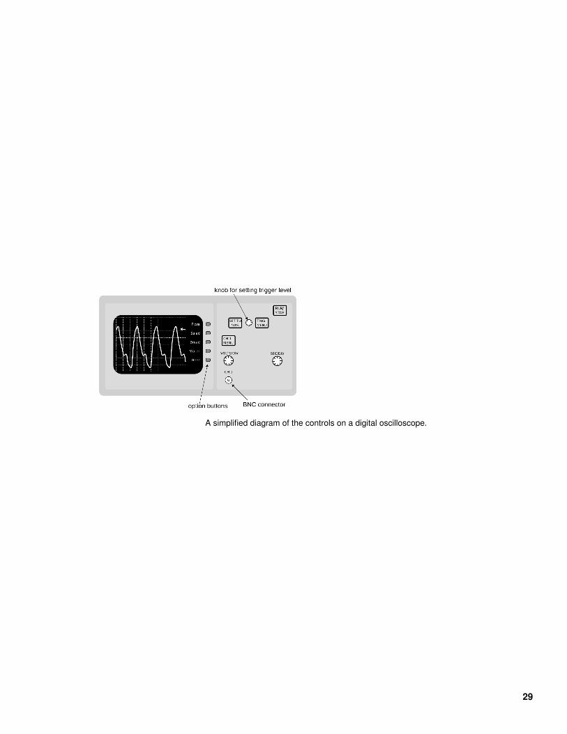
A simplified diagram of the controls on a digital oscilloscope.

29

7 Electromagnetism

Apparatusoscilloscope (Tektronix TDS 1001B) . . . . . . 1/groupmicrophone (RS 33-1067) . . . . . . . . . . . . . for 6 groupsmicrophone (Shure C606) . . . . . . . . . . . . . . for 1 groupvarious tuning forks, mounted on wooden boxessolenoid (Heath) . . . . . . . . . . . . . . . . . . . . . . . . . . 1/group2-meter wire with banana plugs . . . . . . . . . . .1/groupmagnet (stack of 6 Nd) . . . . . . . . . . . . . . . . . . . 1/groupmasking tapestring

GoalsLearn to use an oscilloscope.

Observe electric fields induced by changing mag-netic fields.

Build a generator.

Discover Lenz’s law.

IntroductionPhysicists hate complication, and when physicist Mich-ael Faraday was first learning physics in the early19th century, an embarrassingly complex aspect ofthe science was the multiplicity of types of forces.Friction, normal forces, gravity, electric forces, mag-netic forces, surface tension — the list went on andon. Today, 200 years later, ask a physicist to enu-merate the fundamental forces of nature and themost likely response will be “four: gravity, electro-magnetism, the strong nuclear force and the weaknuclear force.” Part of the simplification came fromthe study of matter at the atomic level, which showedthat apparently unrelated forces such as friction, nor-mal forces, and surface tension were all manifesta-tions of electrical forces among atoms. The otherbig simplification came from Faraday’s experimentalwork showing that electric and magnetic forces wereintimately related in previously unexpected ways, sointimately related in fact that we now refer to thetwo sets of force-phenomena under a single term,“electromagnetism.”

Even before Faraday, Oersted had shown that therewas at least some relationship between electric and

magnetic forces. An electrical current creates a mag-netic field, and magnetic fields exert forces on anelectrical current. In other words, electric forcesare forces of charges acting on charges, and mag-netic forces are forces of moving charges on movingcharges. (Even the magnetic field of a bar magnet isdue to currents, the currents created by the orbitingelectrons in its atoms.)

Faraday took Oersted’s work a step further, andshowed that the relationship between electricity andmagnetism was even deeper. He showed that a chang-ing electric field produces a magnetic field, and achanging magnetic field produces an electric field.Faraday’s work forms the basis for such technologiesas the transformer, the electric guitar, the trans-former, and generator, and the electric motor. Italso led to the understanding of light as an electro-magnetic wave.

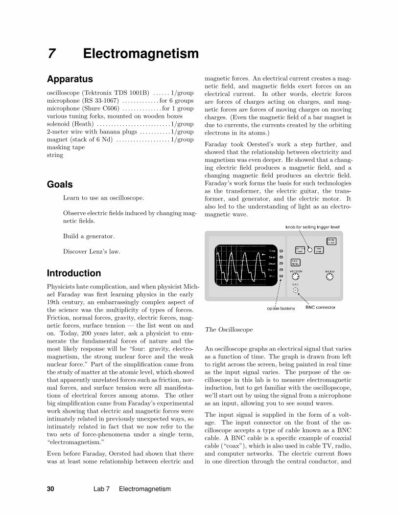
The Oscilloscope

An oscilloscope graphs an electrical signal that variesas a function of time. The graph is drawn from leftto right across the screen, being painted in real timeas the input signal varies. The purpose of the os-cilloscope in this lab is to measure electromagneticinduction, but to get familiar with the oscillopscope,we’ll start out by using the signal from a microphoneas an input, allowing you to see sound waves.

The input signal is supplied in the form of a volt-age. The input connector on the front of the os-cilloscope accepts a type of cable known as a BNCcable. A BNC cable is a specific example of coaxialcable (“coax”), which is also used in cable TV, radio,and computer networks. The electric current flowsin one direction through the central conductor, and

30 Lab 7 Electromagnetism

returns in the opposite direction through the outsideconductor, completing the circuit. The outside con-ductor is normally kept at ground, and also serves asshielding against radio interference. The advantageof coaxial cable is that it is capable of transmittingrapidly varying signals without distortion.

Most of the voltages we wish to measure are not bigenough to use directly for the vertical deflection volt-age, so the oscilloscope actually amplifies the inputvoltage, i.e., the small input voltage is used to con-trol a much larger voltage generated internally. Theamount of amplification is controlled with a knob onthe front of the scope. For instance, setting the knobon 1 mV selects an amplification such that 1 mV atthe input deflects the electron beam by one squareof the 1-cm grid. Each 1-cm division is referred toas a “division.”

The Time Base and Triggering

Since the X axis represents time, there also has tobe a way to control the time scale, i.e., how fastthe imaginary “penpoint” sweeps across the screen.For instance, setting the knob on 10 ms causes it tosweep across one square in 10 ms. This is known asthe time base.

In the figure, suppose the time base is 10 ms. Thescope has 10 divisions, so the total time required forthe beam to sweep from left to right would be 100ms. This is far too short a time to allow the user

to examine the graph. The oscilloscope has a built-in method of overcoming this problem, which workswell for periodic (repeating) signals. The amountof time required for a periodic signal to perform itspattern once is called the period. With a periodicsignal, all you really care about seeing what one pe-riod or a few periods in a row look like — once you’veseen one, you’ve seen them all. The scope displaysone screenful of the signal, and then keeps on over-laying more and more copies of the wave on top ofthe original one. Each trace is erased when the nextone starts, but is being overwritten continually bylater, identical copies of the wave form. You simplysee one persistent trace.

How does the scope know when to start a new trace?If the time for one sweep across the screen just hap-pened to be exactly equal to, say, four periods of thesignal, there would be no problem. But this is un-likely to happen in real life — normally the secondtrace would start from a different point in the wave-form, producing an offset copy of the wave. Thou-sands of traces per second would be superimposedon the screen, each shifted horizontally by a differ-ent amount, and you would only see a blurry bandof light.

To make sure that each trace starts from the samepoint in the waveform, the scope has a triggering cir-cuit. You use a knob to set a certain voltage level,the trigger level, at which you want to start eachtrace. The scope waits for the input to move acrossthe trigger level, and then begins a trace. Once thattrace is complete, it pauses until the input crossesthe trigger level again. To make extra sure that it isreally starting over again from the same point in thewaveform, you can also specify whether you want tostart on an increasing voltage or a decreasing volt-age — otherwise there would always be at least twopoints in a period where the voltage crossed yourtrigger level.

SetupTo start with, we’ll use a sine wave generator, whichmakes a voltage that varies sinusoidally with time.This gives you a convenient signal to work with whileyou get the scope working.

The figure on the preceding page is a simplified draw-ing of the front panel of a digital oscilloscope, show-ing only the most important controls you’ll need forthis lab. When you turn on the oscilloscope, it willtake a while to start up.

31

Preliminaries:

Press DEFAULT SETUP.

Use the SEC/DIV knob to put the time baseon something reasonable compared to the pe-riod of the signal you’re looking at. The timebase is displayed on the screen, e.g., 10 ms/div,or 1 s/div.

Use the VOLTS/DIV knob to put the voltagescale (Y axis) on a reasonable scale comparedto the amplitude of the signal you’re lookingat.

The scope has two channels, i.e., it can ac-cept input through two BNC connectors anddisplay both or either. You’ll only be usingchannel 1, which is the only one represented inthe simplified drawing. By default, the oscil-loscope draws graphs of both channels’ inputs;to get rid of ch. 2, hold down the CH 2 MENUbutton (not shown in the diagram) for a coupleof seconds. You also want to make sure thatthe scope is triggering on CH 1, rather thanCH 2. To do that, press the TRIG MENUbutton, and use an option button to select CH1 as the source. Set the triggering mode to nor-mal, which is the mode in which the triggeringworks as I’ve described above. If the triggerlevel is set to a level that the signal never ac-tually reaches, you can play with the knob thatsets the trigger level until you get something.A quick and easy way to do this without trialand error is to use the SET TO 50% button,which automatically sets the trigger level tomidway between the top and bottom peaks ofthe signal.

You want to select AC, not DC or GND, onthe channel you’re using. You are looking ata voltage that is alternating, creating an al-ternating current, “AC.” The “DC” setting isonly necessary when dealing with constant orvery slowly varying voltages. The “GND” sim-ply draws a graph using y = 0, which is onlyuseful in certain situations, such as when youcan’t find the trace. To select AC, press theCH 1 MENU button, and select AC coupling.

Observe the effect of changing the voltage scale andtime base on the scope. Try changing the frequencyand amplitude on the sine wave generator.

You can freeze the display by pressing RUN/STOP,and then unfreeze it by pressing the button again.

Preliminary ObservationsNow try observing signals from the microphone.

Once you have your setup working, try measuringthe period and frequency of the sound from a tuningfork, and make sure your result for the frequency isthe same as what’s written on the tuning fork.

Qualitative ObservationsIn this lab you will use a permanent magnet to pro-duce changing magnetic fields. This causes an elec-tric field to be induced, which you will detect usinga solenoid (spool of wire) connected to an oscillo-scope. The electric field drives electrons around thesolenoid, producing a current which is detected bythe oscilloscope.

Note that although I’ve described the standard wayof triggering a scope, when the time base is verylong, triggering becomes unnecessary. These scopesare programmed so that when the time base is verylong, they simply continuously display traces.

A A constant magnetic field

Do you detect any signal on the oscilloscope whenthe magnet is simply placed at rest inside the solenoid?Try the most sensitive voltage scale.

B A changing magnetic field

Do you detect any signal when you move the magnetor wiggle it inside the solenoid or near it? Whathappens if you change the speed at which you movethe magnet?

C Moving the solenoid

What happens if you hold the magnet still and movethe solenoid?

The poles of the magnet are its flat faces. In laterparts of the lab you will need to know which is north.Determine this now by hanging it from a string andseeing how it aligns itself with the Earth’s field. Thepole that points north is called the north pole of themagnet. The field pattern funnels into the body ofthe magnet through its south pole, and reemerges atits north pole.

D A generator

Tape the magnet securely to the eraser end of a pen-cil so that its flat face (one of its two poles) is like thehead of a hammer, and mark the north and southpoles of the magnet for later reference. Spin the pen-cil near the solenoid and observe the induced signal.


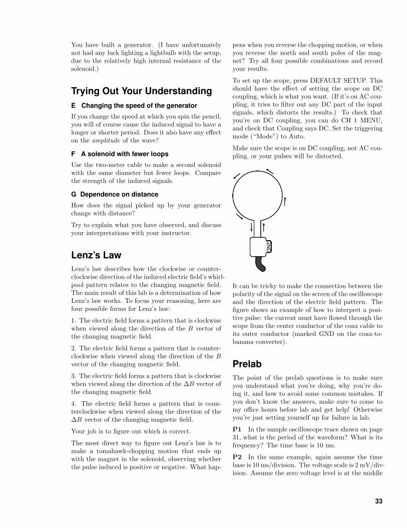
You have built a generator. (I have unfortunatelynot had any luck lighting a lightbulb with the setup,due to the relatively high internal resistance of thesolenoid.)

Trying Out Your UnderstandingE Changing the speed of the generator

If you change the speed at which you spin the pencil,you will of course cause the induced signal to have alonger or shorter period. Does it also have any effecton the amplitude of the wave?

F A solenoid with fewer loops

Use the two-meter cable to make a second solenoidwith the same diameter but fewer loops. Comparethe strength of the induced signals.

G Dependence on distance

How does the signal picked up by your generatorchange with distance?

Try to explain what you have observed, and discussyour interpretations with your instructor.

Lenz’s LawLenz’s law describes how the clockwise or counter-clockwise direction of the induced electric field’s whirl-pool pattern relates to the changing magnetic field.The main result of this lab is a determination of howLenz’s law works. To focus your reasoning, here arefour possible forms for Lenz’s law:

1. The electric field forms a pattern that is clockwisewhen viewed along the direction of the B vector ofthe changing magnetic field.

2. The electric field forms a pattern that is counter-clockwise when viewed along the direction of the Bvector of the changing magnetic field.

3. The electric field forms a pattern that is clockwisewhen viewed along the direction of the ∆B vector ofthe changing magnetic field.

4. The electric field forms a pattern that is coun-terclockwise when viewed along the direction of the∆B vector of the changing magnetic field.

Your job is to figure out which is correct.

The most direct way to figure out Lenz’s law is tomake a tomahawk-chopping motion that ends upwith the magnet in the solenoid, observing whetherthe pulse induced is positive or negative. What hap-

pens when you reverse the chopping motion, or whenyou reverse the north and south poles of the mag-net? Try all four possible combinations and recordyour results.

To set up the scope, press DEFAULT SETUP. Thisshould have the effect of setting the scope on DCcoupling, which is what you want. (If it’s on AC cou-pling, it tries to filter out any DC part of the inputsignals, which distorts the results.) To check thatyou’re on DC coupling, you can do CH 1 MENU,and check that Coupling says DC. Set the triggeringmode (“Mode”) to Auto.

Make sure the scope is on DC coupling, not AC cou-pling, or your pulses will be distorted.

It can be tricky to make the connection between thepolarity of the signal on the screen of the oscilloscopeand the direction of the electric field pattern. Thefigure shows an example of how to interpret a posi-tive pulse: the current must have flowed through thescope from the center conductor of the coax cable toits outer conductor (marked GND on the coax-to-banana converter).


P1 In the sample oscilloscope trace shown on page31, what is the period of the waveform? What is itsfrequency? The time base is 10 ms.

P2 In the same example, again assume the timebase is 10 ms/division. The voltage scale is 2 mV/div-ision. Assume the zero voltage level is at the middle

33

of the vertical scale. (The whole graph can actuallybe shifted up and down using a knob called “posi-tion.”) What is the trigger level currently set to? Ifthe trigger level was changed to 2 mV, what wouldhappen to the trace?

P3 Referring to the chapter of your textbook onsound, which of the following would be a reasonabletime base to use for an audio-frequency signal? 10ns, 1µ s, 1 ms, 1 s

P4 Does the oscilloscope show you the signal’s pe-riod, or its wavelength? Explain. [Skip this questionif you’re in Physics 222.]

P5 The time-scale for all the signals is determinedby the fact that you’re wiggling and waving the mag-net by hand, so what’s a reasonable order of magni-tude to choose for the time base on the oscilloscope?[Skip this question if you’re in Physics 222.]

Self-CheckDetermine which version of Lenz’s law is correct.


35

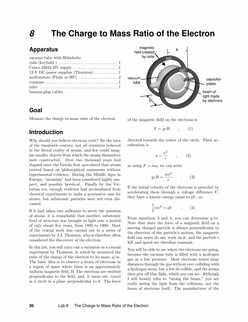
8 The Charge to Mass Ratio of the Electron

Apparatusvacuum tube with Helmholtzcoils (Leybold ) . . . . . . . . . . . . . . . . . . . . . . . . . . . . . . . . . 1Cenco 33034 HV supply . . . . . . . . . . . . . . . . . . . . . . . . . 112-V DC power supplies (Thornton) . . . . . . . . . . . . . 1multimeters (Fluke or HP) . . . . . . . . . . . . . . . . . . . . . . 2compass . . . . . . . . . . . . . . . . . . . . . . . . . . . . . . . . . . . . . . . . . 1ruler . . . . . . . . . . . . . . . . . . . . . . . . . . . . . . . . . . . . . . . . . . . . 1banana-plug cables

GoalMeasure the charge-to-mass ratio of the electron.

IntroductionWhy should you believe electrons exist? By the turnof the twentieth century, not all scientists believedin the literal reality of atoms, and few could imag-ine smaller objects from which the atoms themselveswere constructed. Over two thousand years hadelapsed since the Greeks first speculated that atomsexisted based on philosophical arguments withoutexperimental evidence. During the Middle Ages inEurope, “atomism” had been considered highly sus-pect, and possibly heretical. Finally by the Vic-torian era, enough evidence had accumulated fromchemical experiments to make a persuasive case foratoms, but subatomic particles were not even dis-cussed.

If it had taken two millennia to settle the questionof atoms, it is remarkable that another, subatomiclevel of structure was brought to light over a periodof only about five years, from 1895 to 1900. Mostof the crucial work was carried out in a series ofexperiments by J.J. Thomson, who is therefore oftenconsidered the discoverer of the electron.

In this lab, you will carry out a variation on a crucialexperiment by Thomson, in which he measured theratio of the charge of the electron to its mass, q/m.The basic idea is to observe a beam of electrons ina region of space where there is an approximatelyuniform magnetic field, B. The electrons are emittedperpendicular to the field, and, it turns out, travelin a circle in a plane perpendicular to it. The force

of the magnetic field on the electrons is

F = qvB , (1)

directed towards the center of the circle. Their ac-celeration is

a =v2

r, (2)

so using F = ma, we can write

qvB =mv2

r. (3)

If the initial velocity of the electrons is provided byaccelerating them through a voltage difference V ,they have a kinetic energy equal to qV , so

1

2mv2 = qV . (4)

From equations 3 and 4, you can determine q/m.Note that since the force of a magnetic field on amoving charged particle is always perpendicular tothe direction of the particle’s motion, the magneticfield can never do any work on it, and the particle’sKE and speed are therefore constant.

You will be able to see where the electrons are going,because the vacuum tube is filled with a hydrogengas at a low pressure. Most electrons travel largedistances through the gas without ever colliding witha hydrogen atom, but a few do collide, and the atomsthen give off blue light, which you can see. AlthoughI will loosely refer to “seeing the beam,” you arereally seeing the light from the collisions, not thebeam of electrons itself. The manufacturer of the

36 Lab 8 The Charge to Mass Ratio of the Electron

tube has put in just enough gas to make the beamvisible; more gas would make a brighter beam, butwould cause it to spread out and become too broadto measure it precisely.

The field is supplied by an electromagnet consistingof two circular coils, each with 130 turns of wire(the same on all the tubes we have). The coils areplaced on the same axis, with the vacuum tube atthe center. A pair of coils arranged in this type ofgeometry are called Helmholtz coils. Such a setupprovides a nearly uniform field in a large volumeof space between the coils, and that space is moreaccessible than the inside of a solenoid.

Safety

You will use the Cenco high-voltage supply to makea DC voltage of about 300 V . Two things automat-ically keep this from being very dangerous:

Several hundred DC volts are far less danger-ous than a similar AC voltage. The householdAC voltages of 110 and 220 V are more dan-gerous because AC is more readily conductedby body tissues.

The HV supply will blow a fuse if too muchcurrent flows.

Do the high voltage safety checklist, Appendix 7,tear it out, and turn it in at the beginning of lab. Ifyou don’t understand something, don’t initial thatpoint, and ask your instructor for clarification beforeyou start the lab.

SetupBefore beginning, make sure you do not have anycomputer disks near the apparatus, because the mag-netic field could erase them.

Heater circuit: As with all vacuum tubes, the cath-ode is heated to make it release electrons more easily.There is a separate low-voltage power supply builtinto the high-voltage supply. It has a set of greenplugs that, in different combinations, allow you toget various low voltage values. Use it to supply 6V to the terminals marked “heater” on the vacuumtube. The tube should start to glow.

Electromagnet circuit: Connect the other Thorntonpower supply, in series with an ammeter, to the ter-minals marked “coil.” The current from this powersupply goes through both coils to make the magnetic

field. Verify that the magnet is working by using itto deflect a nearby compass.

High-voltage circuit: Leave the Cenco HV supplyunplugged. It is really three HV circuits in one box.You’ll be using the circuit that goes up to 500 V.Connect it to the terminals marked “anode.” Askyour instructor to check your circuit. Now plug inthe HV supply and turn up the voltage to 300 V.You should see the electron beam. If you don’t seeanything, try it with the lights dimmed.

ObservationsMake the necessary observations in order to findq/m, carrying out your plan to deal with the effectsof the Earth’s field. The high voltage is supposedto be 300 V, but to get an accurate measurementof what it really is you’ll need to use a multimeterrather than the poorly calibrated meter on the frontof the high voltage supply.

The beam can be measured accurately by using theglass rod inside the tube, which has a centimeterscale marked on it.

Be sure to compute q/m before you leave the lab.That way you’ll know you didn’t forget to measuresomething important, and that your result is reason-able compared to the currently accepted value.

There is a glass rod inside the vacuum tube with acentimeter scale on it, so you can measure the diam-eter d of the beam circle simply by looking at theplace where the glowing beam hits the scale. This ismuch more accurate than holding a ruler up to thetube, because it eliminates the parallax error thatwould be caused by viewing the beam and the ruleralong a line that wasn’t perpendicular to the plane ofthe beam. However, the manufacturing process usedin making these tubes (they’re probably hand-blownby a glass blower) isn’t very precise, and on many ofthe tubes you can easily tell by comparison with thea ruler that, e.g., the 10.0 cm point on the glass rodis not really 10.0 cm away from the hole from whichthe beam emerges. Past students have painstakinglydetermined the appropriate corrections, a, to add tothe observed diameters by the following electricalmethod. If you look at your answer to prelab ques-tion P1, you’ll see that the product Br is always afixed quantity in this experiment. It therefore fol-lows that Id is also supposed to be constant. Theymeasured I and d at two different values of I, anddetermined the correction a that had to be added totheir d values in order to make the two values of Idequal. The results are as follows:

37

serial number a (cm)98-16 0.09849 0.099-08 +0.1599-10 -0.299-17 +0.299-56 +0.3031427 -0.3

If your apparatus is one that hasn’t already had its adetermined, then you should do the necessary mea-surements to calibrate it.


The week before you are to do the lab, briefly famil-iarize yourself visually with the apparatus.

Do the high voltage safety checklist, Appendix 7,tear it out, and turn it in at the beginning of lab. Ifyou don’t understand something, don’t initial thatpoint, and ask your instructor for clarification beforeyou start the lab.

P1 Derive an equation for q/m in terms of V , rand B.

P2 For an electromagnet consisting of a single cir-cular loop of wire of radius b, the field at a point onits axis, at a distance z from the plane of the loop,is given by

B =2πkIb2

c2(b2 + z2)3/2.

Starting from this equation, derive an equation forthe magnetic field at the center of a pair of Helmholtzcoils. Let the number of turns in each coil be N (inour case, N = 130), let their radius be b, and let thedistance between them be h. (In the actual experi-ment, the electrons are never exactly on the axis ofthe Helmholtz coils. In practice, the equation youwill derive is sufficiently accurate as an approxima-tion to the actual field experienced by the electrons.)If you have trouble with this derivation, see your in-structor in his/her office hours.

P3 Find the currently accepted value of q/m forthe electron.

P4 The electrons will be affected by the Earth’smagnetic field, as well as the (larger) field of the

coils. Devise a plan to eliminate, correct for, or atleast estimate the effect of the Earth’s magnetic fieldon your final q/m value.

P5 Of the three circuits involved in this experi-ment, which ones need to be hooked up with theright polarity, and for which ones is the polarity ir-relevant?

P6 What would you infer if you found the beamof electrons formed a helix rather than a circle?

AnalysisDetermine q/m, with error bars.

Answer the following questions:

Q1. Thomson started to become convinced duringhis experiments that the “cathode rays” observedcoming from the cathodes of vacuum tubes werebuilding blocks of atoms — what we now call elec-trons. He then carried out observations with cath-odes made of a variety of metals, and found thatq/m was the same in every case. How would thatobservation serve to test his hypothesis?

Q2. Why is it not possible to determine q and mthemselves, rather than just their ratio, by observingelectrons’ motion in electric or magnetic fields?

Q3. Thomson found that the q/m of an electronwas thousands of times larger than that of ions inelectrolysis. Would this imply that the electrons hadmore charge? Less mass? Would there be no way totell? Explain.

38 Lab 8 The Charge to Mass Ratio of the Electron

39

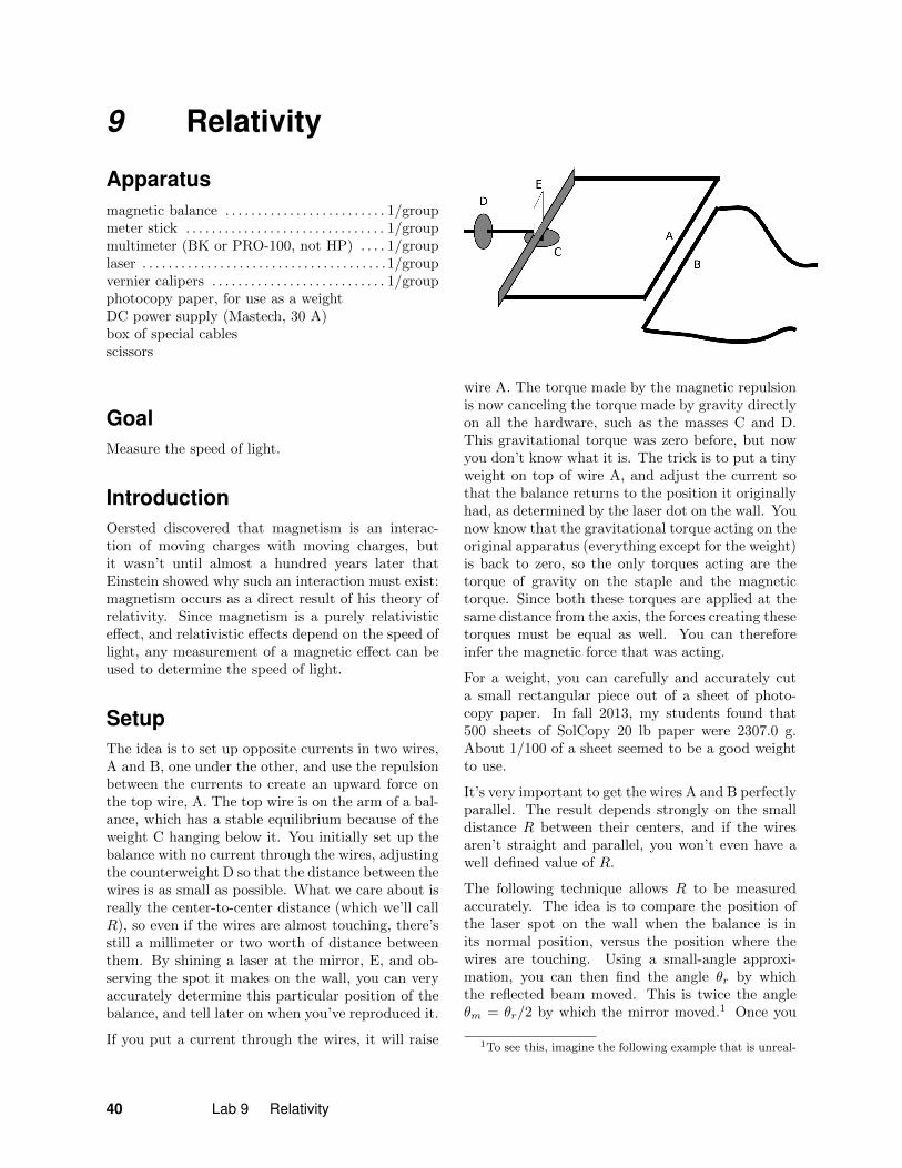
9 Relativity

Apparatusmagnetic balance . . . . . . . . . . . . . . . . . . . . . . . . . 1/groupmeter stick . . . . . . . . . . . . . . . . . . . . . . . . . . . . . . . 1/groupmultimeter (BK or PRO-100, not HP) . . . . 1/grouplaser . . . . . . . . . . . . . . . . . . . . . . . . . . . . . . . . . . . . . .1/groupvernier calipers . . . . . . . . . . . . . . . . . . . . . . . . . . . 1/groupphotocopy paper, for use as a weightDC power supply (Mastech, 30 A)box of special cablesscissors

GoalMeasure the speed of light.

IntroductionOersted discovered that magnetism is an interac-tion of moving charges with moving charges, butit wasn’t until almost a hundred years later thatEinstein showed why such an interaction must exist:magnetism occurs as a direct result of his theory ofrelativity. Since magnetism is a purely relativisticeffect, and relativistic effects depend on the speed oflight, any measurement of a magnetic effect can beused to determine the speed of light.

SetupThe idea is to set up opposite currents in two wires,A and B, one under the other, and use the repulsionbetween the currents to create an upward force onthe top wire, A. The top wire is on the arm of a bal-ance, which has a stable equilibrium because of theweight C hanging below it. You initially set up thebalance with no current through the wires, adjustingthe counterweight D so that the distance between thewires is as small as possible. What we care about isreally the center-to-center distance (which we’ll callR), so even if the wires are almost touching, there’sstill a millimeter or two worth of distance betweenthem. By shining a laser at the mirror, E, and ob-serving the spot it makes on the wall, you can veryaccurately determine this particular position of thebalance, and tell later on when you’ve reproduced it.

If you put a current through the wires, it will raise

wire A. The torque made by the magnetic repulsionis now canceling the torque made by gravity directlyon all the hardware, such as the masses C and D.This gravitational torque was zero before, but nowyou don’t know what it is. The trick is to put a tinyweight on top of wire A, and adjust the current sothat the balance returns to the position it originallyhad, as determined by the laser dot on the wall. Younow know that the gravitational torque acting on theoriginal apparatus (everything except for the weight)is back to zero, so the only torques acting are thetorque of gravity on the staple and the magnetictorque. Since both these torques are applied at thesame distance from the axis, the forces creating thesetorques must be equal as well. You can thereforeinfer the magnetic force that was acting.

For a weight, you can carefully and accurately cuta small rectangular piece out of a sheet of photo-copy paper. In fall 2013, my students found that500 sheets of SolCopy 20 lb paper were 2307.0 g.About 1/100 of a sheet seemed to be a good weightto use.

It’s very important to get the wires A and B perfectlyparallel. The result depends strongly on the smalldistance R between their centers, and if the wiresaren’t straight and parallel, you won’t even have awell defined value of R.

The following technique allows R to be measuredaccurately. The idea is to compare the position ofthe laser spot on the wall when the balance is inits normal position, versus the position where thewires are touching. Using a small-angle approxi-mation, you can then find the angle θr by whichthe reflected beam moved. This is twice the angleθm = θr/2 by which the mirror moved.1 Once you

1To see this, imagine the following example that is unreal-

40 Lab 9 Relativity

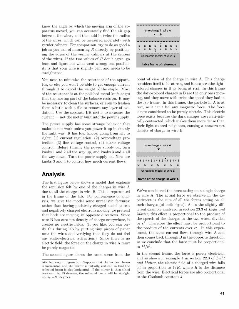
know the angle by which the moving arm of the ap-paratus moved, you can accurately find the air gapbetween the wires, and then add in twice the radiusof the wires, which can be measured accurately withvernier calipers. For comparison, try to do as good ajob as you can of measuring R directly by position-ing the edges of the vernier calipers at the centersof the wires. If the two values of R don’t agree, goback and figure out what went wrong; one possibil-ity is that your wire is slightly bent and needs to bestraightened.

You need to minimize the resistance of the appara-tus, or else you won’t be able to get enough currentthrough it to cancel the weight of the staple. Mostof the resistance is at the polished metal knife-edgesthat the moving part of the balance rests on. It maybe necessary to clean the surfaces, or even to freshenthem a little with a file to remove any layer of oxi-dation. Use the separate BK meter to measure thecurrent — not the meter built into the power supply.

The power supply has some strange behavior thatmakes it not work unless you power it up in exactlythe right way. It has four knobs, going from left toright: (1) current regulation, (2) over-voltage pro-tection, (3) fine voltage control, (4) coarse voltagecontrol. Before turning the power supply on, turnknobs 1 and 2 all the way up, and knobs 3 and 4 allthe way down. Turn the power supply on. Now useknobs 3 and 4 to control how much current flows.

AnalysisThe first figure below shows a model that explainsthe repulsion felt by one of the charges in wire Adue to all the charges in wire B. This is representedin the frame of the lab. For convenience of anal-ysis, we give the model some unrealistic features:rather than having positively charged nuclei at restand negatively charged electrons moving, we pretendthat both are moving, in opposite directions. Sincewire B has zero net density of charge everywhere, itcreates no electric fields. (If you like, you can ver-ify this during lab by putting tiny pieces of papernear the wires and verifying that they do not feelany static-electrical attraction.) Since there is noelectric field, the force on the charge in wire A mustbe purely magnetic.

The second figure shows the same scene from the

istic but easy to figure out. Suppose that the incident beamis horizontal, and the mirror is initially vertical, so that thereflected beam is also horizontal. If the mirror is then tiltedbackward by 45 degrees, the reflected beam will be straightup, θr = 90 degrees.

point of view of the charge in wire A. This chargeconsiders itself to be at rest, and it also sees the light-colored charges in B as being at rest. In this framethe dark-colored charges in B are the only ones mov-ing, and they move with twice the speed they had inthe lab frame. In this frame, the particle in A is atrest, so it can’t feel any magnetic force. The forceis now considered to be purely electric. This electricforce exists because the dark charges are relativisti-cally contracted, which makes them more dense thantheir light-colored neighbors, causing a nonzero netdensity of charge in wire B.

We’ve considered the force acting on a single chargein wire A. The actual force we observe in the ex-periment is the sum of all the forces acting on allsuch charges (of both signs). As in the slightly dif-ferent example analyzed in section 23.3 of Light andMatter, this effect is proportional to the product ofthe speeds of the charges in the two wires, dividedby c2. Therefore the effect must be proportional tothe product of the currents over c2. In this exper-iment, the same current flows through wire A andthen comes back through B in the opposite direction,so we conclude that the force must be proportionalto I2/c2.

In the second frame, the force is purely electrical,and as shown in example 4 in section 22.3 of Lightand Matter, the electric field of a charged wire fallsoff in proportion to 1/R, where R is the distancefrom the wire. Electrical forces are also proportionalto the Coulomb constant k.

41

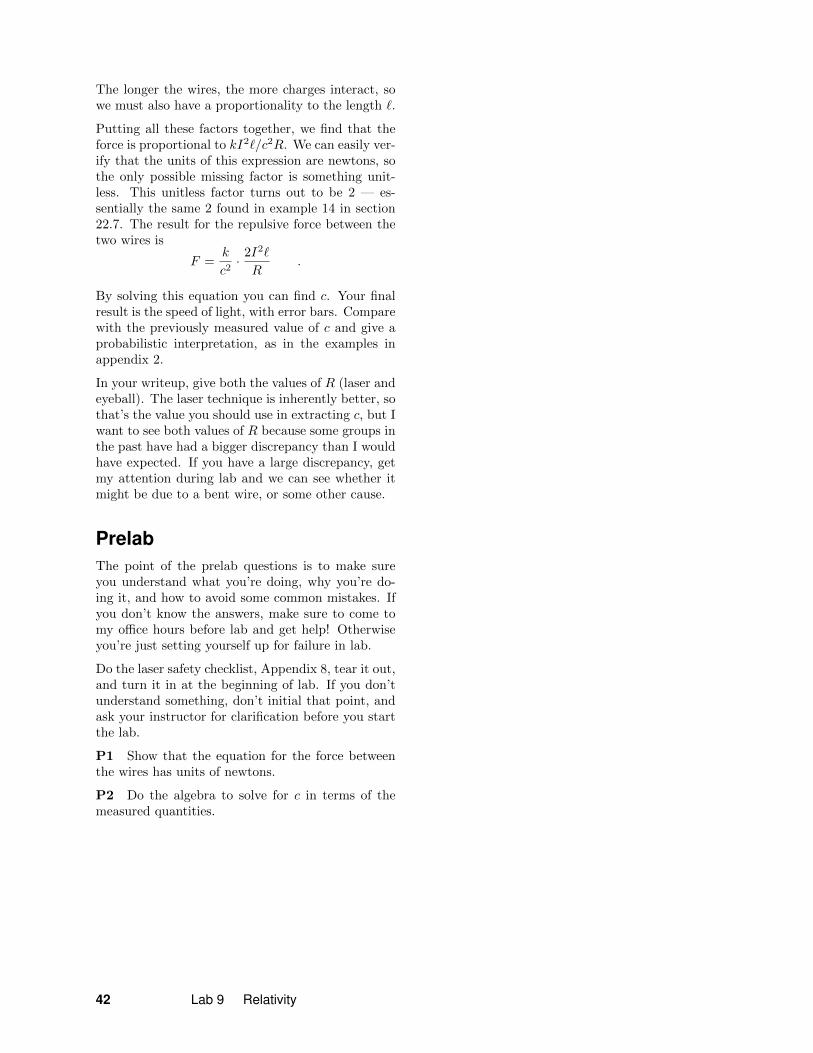
The longer the wires, the more charges interact, sowe must also have a proportionality to the length `.

Putting all these factors together, we find that theforce is proportional to kI2`/c2R. We can easily ver-ify that the units of this expression are newtons, sothe only possible missing factor is something unit-less. This unitless factor turns out to be 2 — es-sentially the same 2 found in example 14 in section22.7. The result for the repulsive force between thetwo wires is

F =k

c2· 2I2`

R.

By solving this equation you can find c. Your finalresult is the speed of light, with error bars. Comparewith the previously measured value of c and give aprobabilistic interpretation, as in the examples inappendix 2.

In your writeup, give both the values of R (laser andeyeball). The laser technique is inherently better, sothat’s the value you should use in extracting c, but Iwant to see both values of R because some groups inthe past have had a bigger discrepancy than I wouldhave expected. If you have a large discrepancy, getmy attention during lab and we can see whether itmight be due to a bent wire, or some other cause.


Do the laser safety checklist, Appendix 8, tear it out,and turn it in at the beginning of lab. If you don’tunderstand something, don’t initial that point, andask your instructor for clarification before you startthe lab.

P1 Show that the equation for the force betweenthe wires has units of newtons.

P2 Do the algebra to solve for c in terms of themeasured quantities.

42 Lab 9 Relativity

43

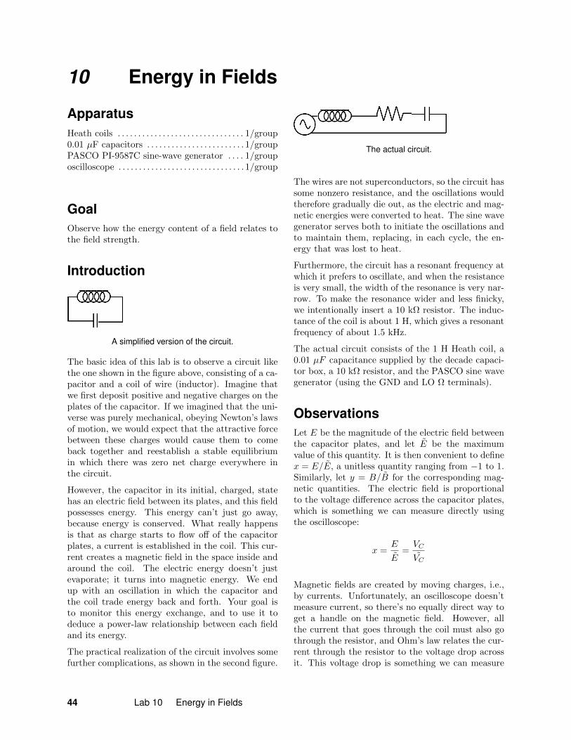
10 Energy in Fields

ApparatusHeath coils . . . . . . . . . . . . . . . . . . . . . . . . . . . . . . . 1/group0.01 µF capacitors . . . . . . . . . . . . . . . . . . . . . . . . 1/groupPASCO PI-9587C sine-wave generator . . . . 1/grouposcilloscope . . . . . . . . . . . . . . . . . . . . . . . . . . . . . . . 1/group

GoalObserve how the energy content of a field relates tothe field strength.

Introduction

A simplified version of the circuit.

The basic idea of this lab is to observe a circuit likethe one shown in the figure above, consisting of a ca-pacitor and a coil of wire (inductor). Imagine thatwe first deposit positive and negative charges on theplates of the capacitor. If we imagined that the uni-verse was purely mechanical, obeying Newton’s lawsof motion, we would expect that the attractive forcebetween these charges would cause them to comeback together and reestablish a stable equilibriumin which there was zero net charge everywhere inthe circuit.

However, the capacitor in its initial, charged, statehas an electric field between its plates, and this fieldpossesses energy. This energy can’t just go away,because energy is conserved. What really happensis that as charge starts to flow off of the capacitorplates, a current is established in the coil. This cur-rent creates a magnetic field in the space inside andaround the coil. The electric energy doesn’t justevaporate; it turns into magnetic energy. We endup with an oscillation in which the capacitor andthe coil trade energy back and forth. Your goal isto monitor this energy exchange, and to use it todeduce a power-law relationship between each fieldand its energy.

The practical realization of the circuit involves somefurther complications, as shown in the second figure.

The actual circuit.

The wires are not superconductors, so the circuit hassome nonzero resistance, and the oscillations wouldtherefore gradually die out, as the electric and mag-netic energies were converted to heat. The sine wavegenerator serves both to initiate the oscillations andto maintain them, replacing, in each cycle, the en-ergy that was lost to heat.

Furthermore, the circuit has a resonant frequency atwhich it prefers to oscillate, and when the resistanceis very small, the width of the resonance is very nar-row. To make the resonance wider and less finicky,we intentionally insert a 10 kΩ resistor. The induc-tance of the coil is about 1 H, which gives a resonantfrequency of about 1.5 kHz.

The actual circuit consists of the 1 H Heath coil, a0.01 µF capacitance supplied by the decade capaci-tor box, a 10 kΩ resistor, and the PASCO sine wavegenerator (using the GND and LO Ω terminals).

ObservationsLet E be the magnitude of the electric field betweenthe capacitor plates, and let E be the maximumvalue of this quantity. It is then convenient to definex = E/E, a unitless quantity ranging from −1 to 1.Similarly, let y = B/B for the corresponding mag-netic quantities. The electric field is proportionalto the voltage difference across the capacitor plates,which is something we can measure directly usingthe oscilloscope:

x =E

E=VC

VC

Magnetic fields are created by moving charges, i.e.,by currents. Unfortunately, an oscilloscope doesn’tmeasure current, so there’s no equally direct way toget a handle on the magnetic field. However, allthe current that goes through the coil must also gothrough the resistor, and Ohm’s law relates the cur-rent through the resistor to the voltage drop acrossit. This voltage drop is something we can measure

44 Lab 10 Energy in Fields

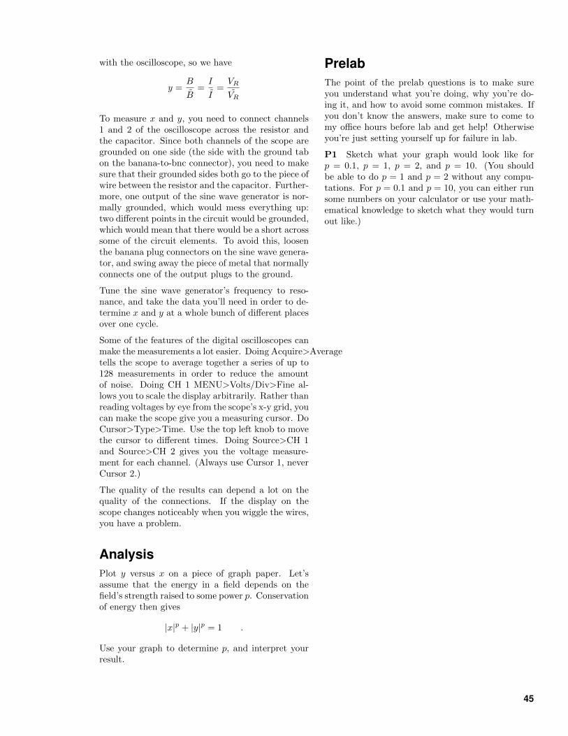
with the oscilloscope, so we have

y =B

B=I

I=VR

VR

To measure x and y, you need to connect channels1 and 2 of the oscilloscope across the resistor andthe capacitor. Since both channels of the scope aregrounded on one side (the side with the ground tabon the banana-to-bnc connector), you need to makesure that their grounded sides both go to the piece ofwire between the resistor and the capacitor. Further-more, one output of the sine wave generator is nor-mally grounded, which would mess everything up:two different points in the circuit would be grounded,which would mean that there would be a short acrosssome of the circuit elements. To avoid this, loosenthe banana plug connectors on the sine wave genera-tor, and swing away the piece of metal that normallyconnects one of the output plugs to the ground.

Tune the sine wave generator’s frequency to reso-nance, and take the data you’ll need in order to de-termine x and y at a whole bunch of different placesover one cycle.

Some of the features of the digital oscilloscopes canmake the measurements a lot easier. Doing Acquire>Averagetells the scope to average together a series of up to128 measurements in order to reduce the amountof noise. Doing CH 1 MENU>Volts/Div>Fine al-lows you to scale the display arbitrarily. Rather thanreading voltages by eye from the scope’s x-y grid, youcan make the scope give you a measuring cursor. DoCursor>Type>Time. Use the top left knob to movethe cursor to different times. Doing Source>CH 1and Source>CH 2 gives you the voltage measure-ment for each channel. (Always use Cursor 1, neverCursor 2.)

The quality of the results can depend a lot on thequality of the connections. If the display on thescope changes noticeably when you wiggle the wires,you have a problem.

AnalysisPlot y versus x on a piece of graph paper. Let’sassume that the energy in a field depends on thefield’s strength raised to some power p. Conservationof energy then gives

|x|p + |y|p = 1 .

Use your graph to determine p, and interpret yourresult.


P1 Sketch what your graph would look like forp = 0.1, p = 1, p = 2, and p = 10. (You shouldbe able to do p = 1 and p = 2 without any compu-tations. For p = 0.1 and p = 10, you can either runsome numbers on your calculator or use your math-ematical knowledge to sketch what they would turnout like.)

45

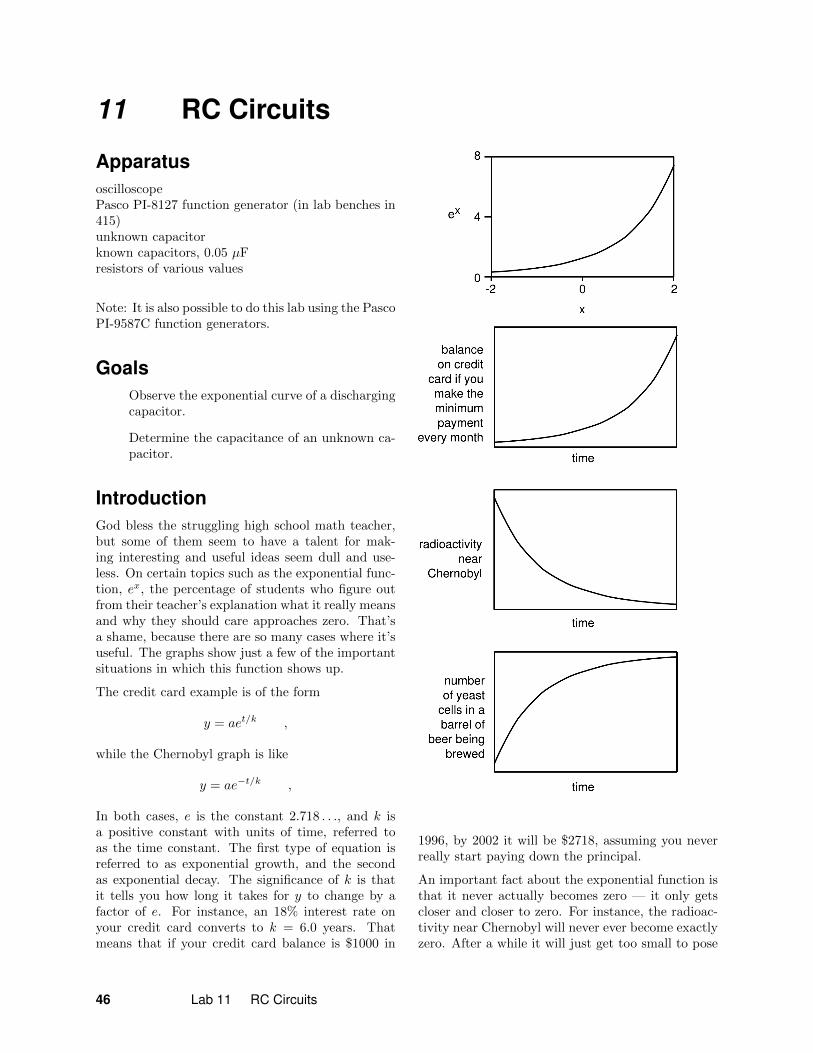
11 RC Circuits

ApparatusoscilloscopePasco PI-8127 function generator (in lab benches in415)unknown capacitorknown capacitors, 0.05 µFresistors of various values

Note: It is also possible to do this lab using the PascoPI-9587C function generators.

GoalsObserve the exponential curve of a dischargingcapacitor.

Determine the capacitance of an unknown ca-pacitor.

IntroductionGod bless the struggling high school math teacher,but some of them seem to have a talent for mak-ing interesting and useful ideas seem dull and use-less. On certain topics such as the exponential func-tion, ex, the percentage of students who figure outfrom their teacher’s explanation what it really meansand why they should care approaches zero. That’sa shame, because there are so many cases where it’suseful. The graphs show just a few of the importantsituations in which this function shows up.

The credit card example is of the form

y = aet/k ,

while the Chernobyl graph is like

y = ae−t/k ,

In both cases, e is the constant 2.718 . . ., and k isa positive constant with units of time, referred toas the time constant. The first type of equation isreferred to as exponential growth, and the secondas exponential decay. The significance of k is thatit tells you how long it takes for y to change by afactor of e. For instance, an 18% interest rate onyour credit card converts to k = 6.0 years. Thatmeans that if your credit card balance is $1000 in

1996, by 2002 it will be $2718, assuming you neverreally start paying down the principal.

An important fact about the exponential function isthat it never actually becomes zero — it only getscloser and closer to zero. For instance, the radioac-tivity near Chernobyl will never ever become exactlyzero. After a while it will just get too small to pose

46 Lab 11 RC Circuits

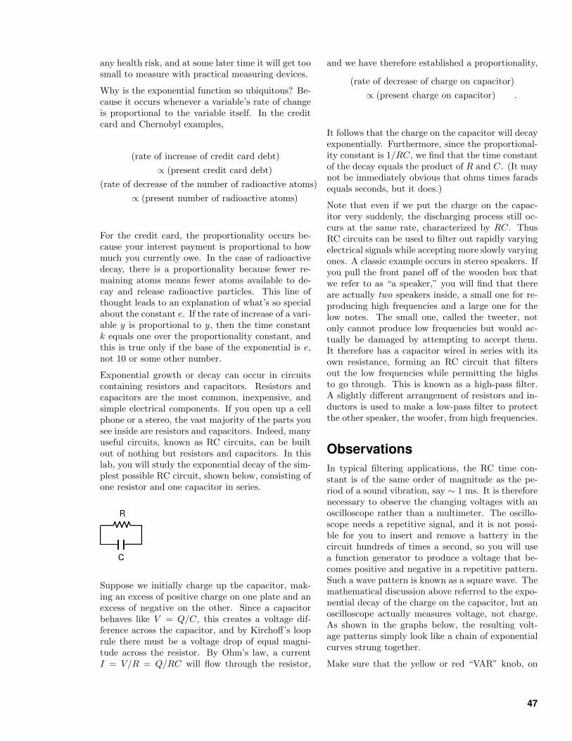
any health risk, and at some later time it will get toosmall to measure with practical measuring devices.

Why is the exponential function so ubiquitous? Be-cause it occurs whenever a variable’s rate of changeis proportional to the variable itself. In the creditcard and Chernobyl examples,

(rate of increase of credit card debt)

∝ (present credit card debt)

(rate of decrease of the number of radioactive atoms)

∝ (present number of radioactive atoms)

For the credit card, the proportionality occurs be-cause your interest payment is proportional to howmuch you currently owe. In the case of radioactivedecay, there is a proportionality because fewer re-maining atoms means fewer atoms available to de-cay and release radioactive particles. This line ofthought leads to an explanation of what’s so specialabout the constant e. If the rate of increase of a vari-able y is proportional to y, then the time constantk equals one over the proportionality constant, andthis is true only if the base of the exponential is e,not 10 or some other number.

Exponential growth or decay can occur in circuitscontaining resistors and capacitors. Resistors andcapacitors are the most common, inexpensive, andsimple electrical components. If you open up a cellphone or a stereo, the vast majority of the parts yousee inside are resistors and capacitors. Indeed, manyuseful circuits, known as RC circuits, can be builtout of nothing but resistors and capacitors. In thislab, you will study the exponential decay of the sim-plest possible RC circuit, shown below, consisting ofone resistor and one capacitor in series.

Suppose we initially charge up the capacitor, mak-ing an excess of positive charge on one plate and anexcess of negative on the other. Since a capacitorbehaves like V = Q/C, this creates a voltage dif-ference across the capacitor, and by Kirchoff’s looprule there must be a voltage drop of equal magni-tude across the resistor. By Ohm’s law, a currentI = V/R = Q/RC will flow through the resistor,

and we have therefore established a proportionality,

(rate of decrease of charge on capacitor)

∝ (present charge on capacitor) .

It follows that the charge on the capacitor will decayexponentially. Furthermore, since the proportional-ity constant is 1/RC, we find that the time constantof the decay equals the product of R and C. (It maynot be immediately obvious that ohms times faradsequals seconds, but it does.)

Note that even if we put the charge on the capac-itor very suddenly, the discharging process still oc-curs at the same rate, characterized by RC. ThusRC circuits can be used to filter out rapidly varyingelectrical signals while accepting more slowly varyingones. A classic example occurs in stereo speakers. Ifyou pull the front panel off of the wooden box thatwe refer to as “a speaker,” you will find that thereare actually two speakers inside, a small one for re-producing high frequencies and a large one for thelow notes. The small one, called the tweeter, notonly cannot produce low frequencies but would ac-tually be damaged by attempting to accept them.It therefore has a capacitor wired in series with itsown resistance, forming an RC circuit that filtersout the low frequencies while permitting the highsto go through. This is known as a high-pass filter.A slightly different arrangement of resistors and in-ductors is used to make a low-pass filter to protectthe other speaker, the woofer, from high frequencies.

ObservationsIn typical filtering applications, the RC time con-stant is of the same order of magnitude as the pe-riod of a sound vibration, say ∼ 1 ms. It is thereforenecessary to observe the changing voltages with anoscilloscope rather than a multimeter. The oscillo-scope needs a repetitive signal, and it is not possi-ble for you to insert and remove a battery in thecircuit hundreds of times a second, so you will usea function generator to produce a voltage that be-comes positive and negative in a repetitive pattern.Such a wave pattern is known as a square wave. Themathematical discussion above referred to the expo-nential decay of the charge on the capacitor, but anoscilloscope actually measures voltage, not charge.As shown in the graphs below, the resulting volt-age patterns simply look like a chain of exponentialcurves strung together.

Make sure that the yellow or red “VAR” knob, on

47

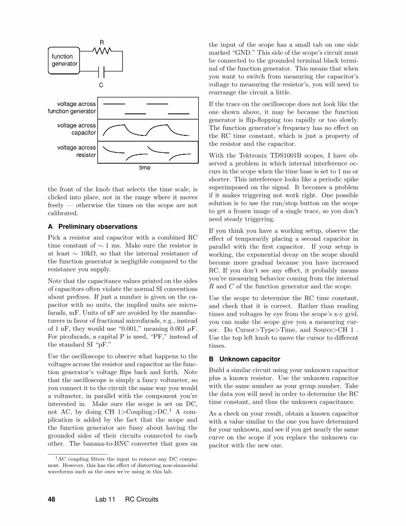
the front of the knob that selects the time scale, isclicked into place, not in the range where it movesfreely — otherwise the times on the scope are notcalibrated.

A Preliminary observations

Pick a resistor and capacitor with a combined RCtime constant of ∼ 1 ms. Make sure the resistor isat least ∼ 10kΩ, so that the internal resistance ofthe function generator is negligible compared to theresistance you supply.

Note that the capacitance values printed on the sidesof capacitors often violate the normal SI conventionsabout prefixes. If just a number is given on the ca-pacitor with no units, the implied units are micro-farads, mF. Units of nF are avoided by the manufac-turers in favor of fractional microfarads, e.g., insteadof 1 nF, they would use “0.001,” meaning 0.001 µF.For picofarads, a capital P is used, “PF,” instead ofthe standard SI “pF.”

Use the oscilloscope to observe what happens to thevoltages across the resistor and capacitor as the func-tion generator’s voltage flips back and forth. Notethat the oscilloscope is simply a fancy voltmeter, soyou connect it to the circuit the same way you woulda voltmeter, in parallel with the component you’reinterested in. Make sure the scope is set on DC,not AC, by doing CH 1>Coupling>DC.1 A com-plication is added by the fact that the scope andthe function generator are fussy about having thegrounded sides of their circuits connected to eachother. The banana-to-BNC converter that goes on

1AC coupling filters the input to remove any DC compo-nent. However, this has the effect of distorting non-sinusoidalwaveforms such as the ones we’re using in this lab.

the input of the scope has a small tab on one sidemarked “GND.” This side of the scope’s circuit mustbe connected to the grounded terminal black termi-nal of the function generator. This means that whenyou want to switch from measuring the capacitor’svoltage to measuring the resistor’s, you will need torearrange the circuit a little.

If the trace on the oscilloscope does not look like theone shown above, it may be because the functiongenerator is flip-flopping too rapidly or too slowly.The function generator’s frequency has no effect onthe RC time constant, which is just a property ofthe resistor and the capacitor.

With the Tektronix TDS1001B scopes, I have ob-served a problem in which internal interference oc-curs in the scope when the time base is set to 1 ms orshorter. This interference looks like a periodic spikesuperimposed on the signal. It becomes a problemif it makes triggering not work right. One possiblesolution is to use the run/stop button on the scopeto get a frozen image of a single trace, so you don’tneed steady triggering.

If you think you have a working setup, observe theeffect of temporarily placing a second capacitor inparallel with the first capacitor. If your setup isworking, the exponential decay on the scope shouldbecome more gradual because you have increasedRC. If you don’t see any effect, it probably meansyou’re measuring behavior coming from the internalR and C of the function generator and the scope.

Use the scope to determine the RC time constant,and check that it is correct. Rather than readingtimes and voltages by eye from the scope’s x-y grid,you can make the scope give you a measuring cur-sor. Do Cursor>Type>Time, and Source>CH 1 .Use the top left knob to move the cursor to differenttimes.

B Unknown capacitor

Build a similar circuit using your unknown capacitorplus a known resistor. Use the unknown capacitorwith the same number as your group number. Takethe data you will need in order to determine the RCtime constant, and thus the unknown capacitance.

As a check on your result, obtain a known capacitorwith a value similar to the one you have determinedfor your unknown, and see if you get nearly the samecurve on the scope if you replace the unknown ca-pacitor with the new one.

48 Lab 11 RC Circuits


P1 Plan how you will determine the capacitanceand what data you will need to take.

AnalysisDetermine the capacitance, with error analysis (ap-pendices 2 and 3).

49

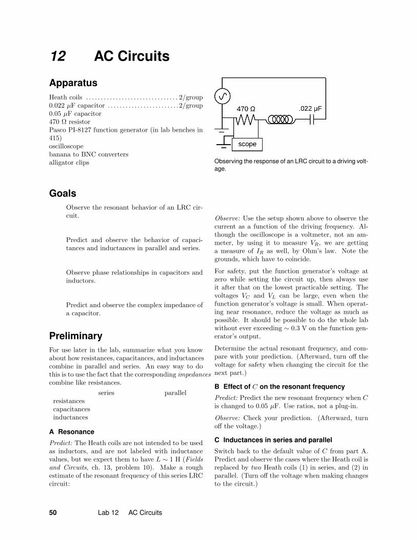
12 AC Circuits

ApparatusHeath coils . . . . . . . . . . . . . . . . . . . . . . . . . . . . . . . 2/group0.022 µF capacitor . . . . . . . . . . . . . . . . . . . . . . . .2/group0.05 µF capacitor470 Ω resistorPasco PI-8127 function generator (in lab benches in415)oscilloscopebanana to BNC convertersalligator clips

GoalsObserve the resonant behavior of an LRC cir-cuit.

Predict and observe the behavior of capaci-tances and inductances in parallel and series.

Observe phase relationships in capacitors andinductors.

Predict and observe the complex impedance ofa capacitor.

PreliminaryFor use later in the lab, summarize what you knowabout how resistances, capacitances, and inductancescombine in parallel and series. An easy way to dothis is to use the fact that the corresponding impedancescombine like resistances.

series parallelresistancescapacitancesinductances

A Resonance

Predict: The Heath coils are not intended to be usedas inductors, and are not labeled with inductancevalues, but we expect them to have L ∼ 1 H (Fieldsand Circuits, ch. 13, problem 10). Make a roughestimate of the resonant frequency of this series LRCcircuit:

Observing the response of an LRC circuit to a driving volt-age.

Observe: Use the setup shown above to observe thecurrent as a function of the driving frequency. Al-though the oscilloscope is a voltmeter, not an am-meter, by using it to measure VR, we are gettinga measure of IR as well, by Ohm’s law. Note thegrounds, which have to coincide.

For safety, put the function generator’s voltage atzero while setting the circuit up, then always useit after that on the lowest practicable setting. Thevoltages VC and VL can be large, even when thefunction generator’s voltage is small. When operat-ing near resonance, reduce the voltage as much aspossible. It should be possible to do the whole labwithout ever exceeding ∼ 0.3 V on the function gen-erator’s output.

Determine the actual resonant frequency, and com-pare with your prediction. (Afterward, turn off thevoltage for safety when changing the circuit for thenext part.)

B Effect of C on the resonant frequency

Predict: Predict the new resonant frequency when Cis changed to 0.05 µF. Use ratios, not a plug-in.

Observe: Check your prediction. (Afterward, turnoff the voltage.)

C Inductances in series and parallel

Switch back to the default value of C from part A.Predict and observe the cases where the Heath coil isreplaced by two Heath coils (1) in series, and (2) inparallel. (Turn off the voltage when making changesto the circuit.)

50 Lab 12 AC Circuits

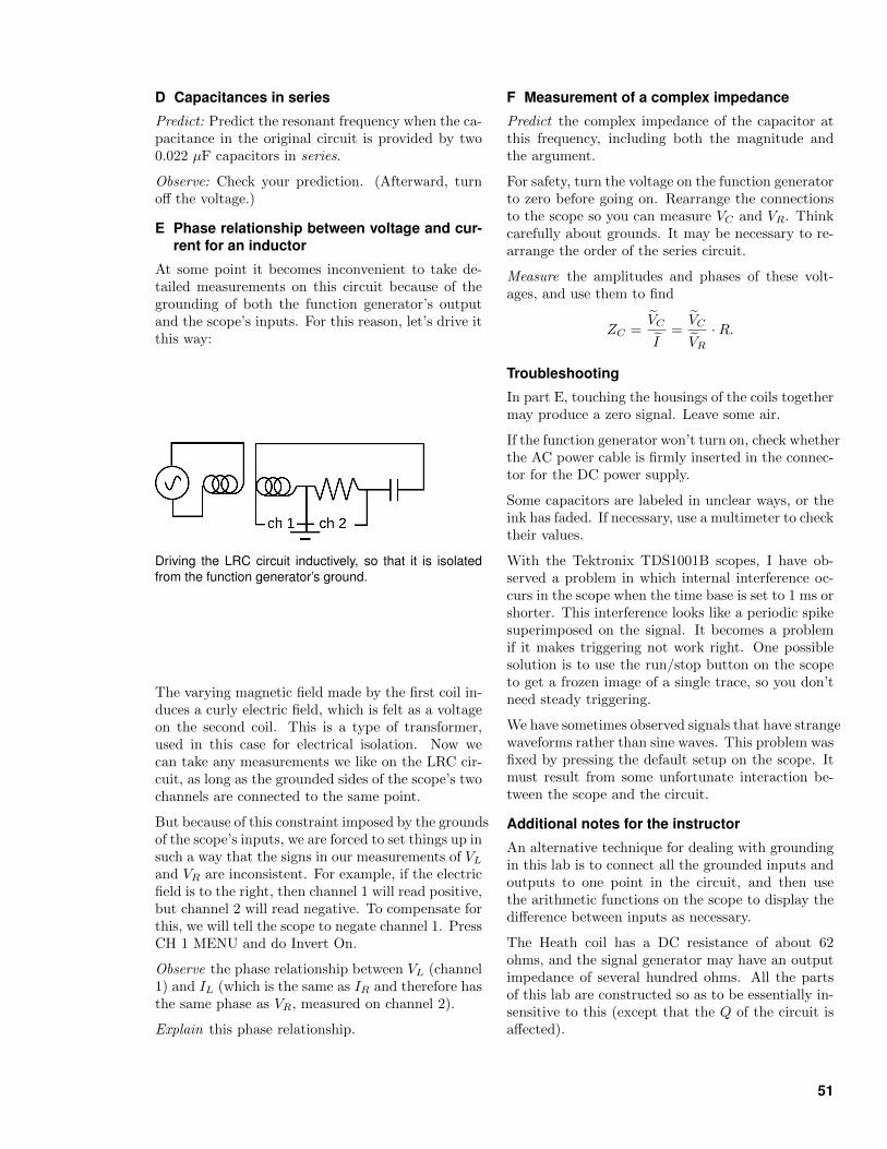
D Capacitances in series

Predict: Predict the resonant frequency when the ca-pacitance in the original circuit is provided by two0.022 µF capacitors in series.

Observe: Check your prediction. (Afterward, turnoff the voltage.)

E Phase relationship between voltage and cur-rent for an inductor

At some point it becomes inconvenient to take de-tailed measurements on this circuit because of thegrounding of both the function generator’s outputand the scope’s inputs. For this reason, let’s drive itthis way:

Driving the LRC circuit inductively, so that it is isolatedfrom the function generator’s ground.

The varying magnetic field made by the first coil in-duces a curly electric field, which is felt as a voltageon the second coil. This is a type of transformer,used in this case for electrical isolation. Now wecan take any measurements we like on the LRC cir-cuit, as long as the grounded sides of the scope’s twochannels are connected to the same point.

But because of this constraint imposed by the groundsof the scope’s inputs, we are forced to set things up insuch a way that the signs in our measurements of VLand VR are inconsistent. For example, if the electricfield is to the right, then channel 1 will read positive,but channel 2 will read negative. To compensate forthis, we will tell the scope to negate channel 1. PressCH 1 MENU and do Invert On.

Observe the phase relationship between VL (channel1) and IL (which is the same as IR and therefore hasthe same phase as VR, measured on channel 2).

Explain this phase relationship.

F Measurement of a complex impedance

Predict the complex impedance of the capacitor atthis frequency, including both the magnitude andthe argument.

For safety, turn the voltage on the function generatorto zero before going on. Rearrange the connectionsto the scope so you can measure VC and VR. Thinkcarefully about grounds. It may be necessary to re-arrange the order of the series circuit.

Measure the amplitudes and phases of these volt-ages, and use them to find

ZC =VC

I=VC

VR·R.

Troubleshooting

In part E, touching the housings of the coils togethermay produce a zero signal. Leave some air.

If the function generator won’t turn on, check whetherthe AC power cable is firmly inserted in the connec-tor for the DC power supply.

Some capacitors are labeled in unclear ways, or theink has faded. If necessary, use a multimeter to checktheir values.

With the Tektronix TDS1001B scopes, I have ob-served a problem in which internal interference oc-curs in the scope when the time base is set to 1 ms orshorter. This interference looks like a periodic spikesuperimposed on the signal. It becomes a problemif it makes triggering not work right. One possiblesolution is to use the run/stop button on the scopeto get a frozen image of a single trace, so you don’tneed steady triggering.

We have sometimes observed signals that have strangewaveforms rather than sine waves. This problem wasfixed by pressing the default setup on the scope. Itmust result from some unfortunate interaction be-tween the scope and the circuit.

Additional notes for the instructor

An alternative technique for dealing with groundingin this lab is to connect all the grounded inputs andoutputs to one point in the circuit, and then usethe arithmetic functions on the scope to display thedifference between inputs as necessary.

The Heath coil has a DC resistance of about 62ohms, and the signal generator may have an outputimpedance of several hundred ohms. All the partsof this lab are constructed so as to be essentially in-sensitive to this (except that the Q of the circuit isaffected).

51

13 Faraday’s Law

ApparatusPasco PI-8127 function generator (in lab benches in415; see note below)solenoid (Heath) 1/group plus a few moreoscilloscope . . . . . . . . . . . . . . . . . . . . . . . . . . . . . . . 1/group100 Ω resistor . . . . . . . . . . . . . . . . . . . . . . . . . . . . 1/groupsecondary coils (see note below)palm-sized pieces of iron or steelmasking taperulers

Notes: It is also probably possible to do this labusing the Pasco PI-9587C function generators, but Ihaven’t tested it.

We have a variety of coils that can be used as sec-ondary coils. The text below describes using a loopmade out of a 4-meter piece of wire. We have abunch of these made up using white wire with ba-nana plugs on the ends. Although these can be madeto work, the signal is rather weak because of thesmall number of turns. We have a set of small rect-angular coils with various numbers of turns, PASCOSF-8617. I’ve successfully used the 3200-turn coil,which produces a big signal. The others have arealso probably usable. I have also made a couple ofhand-wrapped coils for use in this lab.

GoalsObserve electric fields induced by changing mag-netic fields.

Test Faraday’s law.

IntroductionPhysicists hate complication, and when physicist Mi-chael Faraday was first learning physics in the early19th century, an embarrassingly complex aspect ofthe science was the multiplicity of types of forces.Friction, normal forces, gravity, electric forces, mag-netic forces, surface tension — the list went on andon. Today, 200 years later, ask a physicist to enu-merate the fundamental forces of nature and themost likely response will be “four: gravity, electro-magnetism, the strong nuclear force and the weaknuclear force.” Part of the simplification came from

the study of matter at the atomic level, which showedthat apparently unrelated forces such as friction, nor-mal forces, and surface tension were all manifesta-tions of electrical forces among atoms. The otherbig simplification came from Faraday’s experimentalwork showing that electric and magnetic forces wereintimately related in previously unexpected ways, sointimately related in fact that we now refer to thetwo sets of force-phenomena under a single term,“electromagnetism.”

Even before Faraday, Oersted had shown that therewas at least some relationship between electric andmagnetic forces. An electrical current creates a mag-netic field, and magnetic fields exert forces on anelectrical current. In other words, electric forcesare forces of charges acting on charges, and mag-netic forces are forces of moving charges on movingcharges. (Even the magnetic field of a bar magnet isdue to currents, the currents created by the orbitingelectrons in its atoms.)

Faraday took Oersted’s work a step further, andshowed that the relationship between electricity andmagnetism was even deeper. He showed that a chang-ing electric field produces a magnetic field, and achanging magnetic field produces an electric field.Faraday’s law, ∫

E · ` = −dΦB/dt

relates the integral of the electric field around a closedloop to the rate of change of the magnetic flux throughthe loop. It forms the basis for such technologies asthe transformer, the electric guitar, the amplifier,and generator, and the electric motor.

ObservationsA Qualitative Observations

To observe Faraday’s law in action you will first needto produce a varying magnetic field. You can do thisby using a function generator to produce a currentin a solenoid that that varies like a sine wave as afunction of time. The solenoid’s magnetic field willthus also vary sinusoidally.

The emf in Faraday’s law can be observed around aloop of wire positioned inside or close to the solenoid.To make the emf larger and easier to see on an os-

52 Lab 13 Faraday’s Law

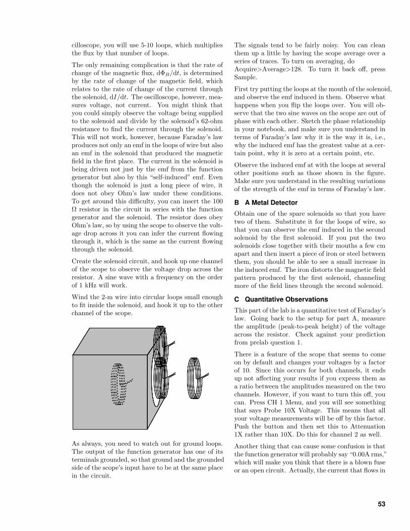
cilloscope, you will use 5-10 loops, which multipliesthe flux by that number of loops.

The only remaining complication is that the rate ofchange of the magnetic flux, dΦB/dt, is determinedby the rate of change of the magnetic field, whichrelates to the rate of change of the current throughthe solenoid, dI/dt. The oscilloscope, however, mea-sures voltage, not current. You might think thatyou could simply observe the voltage being suppliedto the solenoid and divide by the solenoid’s 62-ohmresistance to find the current through the solenoid.This will not work, however, because Faraday’s lawproduces not only an emf in the loops of wire but alsoan emf in the solenoid that produced the magneticfield in the first place. The current in the solenoid isbeing driven not just by the emf from the functiongenerator but also by this “self-induced” emf. Eventhough the solenoid is just a long piece of wire, itdoes not obey Ohm’s law under these conditions.To get around this difficulty, you can insert the 100Ω resistor in the circuit in series with the functiongenerator and the solenoid. The resistor does obeyOhm’s law, so by using the scope to observe the volt-age drop across it you can infer the current flowingthrough it, which is the same as the current flowingthrough the solenoid.

Create the solenoid circuit, and hook up one channelof the scope to observe the voltage drop across theresistor. A sine wave with a frequency on the orderof 1 kHz will work.

Wind the 2-m wire into circular loops small enoughto fit inside the solenoid, and hook it up to the otherchannel of the scope.

As always, you need to watch out for ground loops.The output of the function generator has one of itsterminals grounded, so that ground and the groundedside of the scope’s input have to be at the same placein the circuit.

The signals tend to be fairly noisy. You can cleanthem up a little by having the scope average over aseries of traces. To turn on averaging, doAcquire>Average>128. To turn it back off, pressSample.

First try putting the loops at the mouth of the solenoid,and observe the emf induced in them. Observe whathappens when you flip the loops over. You will ob-serve that the two sine waves on the scope are out ofphase with each other. Sketch the phase relationshipin your notebook, and make sure you understand interms of Faraday’s law why it is the way it is, i.e.,why the induced emf has the greatest value at a cer-tain point, why it is zero at a certain point, etc.

Observe the induced emf at with the loops at severalother positions such as those shown in the figure.Make sure you understand in the resulting variationsof the strength of the emf in terms of Faraday’s law.

B A Metal Detector

Obtain one of the spare solenoids so that you havetwo of them. Substitute it for the loops of wire, sothat you can observe the emf induced in the secondsolenoid by the first solenoid. If you put the twosolenoids close together with their mouths a few cmapart and then insert a piece of iron or steel betweenthem, you should be able to see a small increase inthe induced emf. The iron distorts the magnetic fieldpattern produced by the first solenoid, channelingmore of the field lines through the second solenoid.

C Quantitative Observations

This part of the lab is a quantitative test of Faraday’slaw. Going back to the setup for part A, measurethe amplitude (peak-to-peak height) of the voltageacross the resistor. Check against your predictionfrom prelab question 1.

There is a feature of the scope that seems to comeon by default and changes your voltages by a factorof 10. Since this occurs for both channels, it endsup not affecting your results if you express them asa ratio between the amplitudes measured on the twochannels. However, if you want to turn this off, youcan. Press CH 1 Menu, and you will see somethingthat says Probe 10X Voltage. This means that allyour voltage measurements will be off by this factor.Push the button and then set this to Attenuation1X rather than 10X. Do this for channel 2 as well.

Another thing that can cause some confusion is thatthe function generator will probably say “0.00A rms,”which will make you think that there is a blown fuseor an open circuit. Actually, the current that flows in

53

the solenoid circuit is simply so small that it roundsoff to 0.00 on this readout.

Choose a position for the loops of wire that you thinkwill make it as easy as possible to calculate dΦB/dtaccurately based on knowledge of the variation of thecurrent in the solenoid as a function of time. Put theloops in that position, and measure the amplitude ofthe induced emf. Repeat these measurements witha frequency that is different by a factor of two.

Self-CheckBefore leaving, analyze your results from part C andmake sure you get reasonable agreement with Fara-day’s law.

AnalysisDescribe your observations in parts A and B andinterpret them in terms of Faraday’s law.

Compare your observations in part C quantitativelywith Faraday’s law. The solenoid isn’t very long,so the approximate expression for the interior fieldof a long solenoid isn’t very accurate here. To cor-rect for that, multiply the expression for the field bythe correction factor ζ = (cos θ1 − cos θ2)/2, (Fieldsand Circuits, ch. 11, problem 13), where θ1 and θ2are angles between the axis and the lines connectingthe point of interest to the edges of the solenoid’smouths.

This analysis is horrible to do and to read if you doit all numerically. Let V be the voltage across theresistor and E the emf measured on the secondarycoil. It’s nice to work with the unitless ratio E/V .For your theoretical result, you should be able to ex-press this ratio symbolically in terms of the followingsymbols:

k = Columb constant

c = speed of light

N1 = number of turns in the primary coil

N2 = number of turns in the secondary coil

f = frequency

A = area of the secondary coil

` = length of the primary coil

R = resistance of the resistor

ζ = correction factor for the magnetic field.

Check that the units work. Only plug in numbers atthe end.


P1 Find the theoretical equation for E/V .

54 Lab 13 Faraday’s Law

55

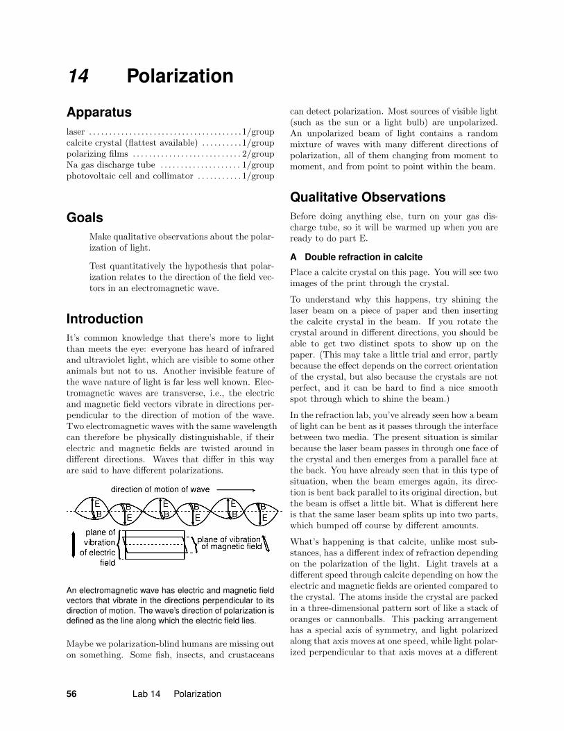
14 Polarization

Apparatuslaser . . . . . . . . . . . . . . . . . . . . . . . . . . . . . . . . . . . . . .1/groupcalcite crystal (flattest available) . . . . . . . . . .1/grouppolarizing films . . . . . . . . . . . . . . . . . . . . . . . . . . . 2/groupNa gas discharge tube . . . . . . . . . . . . . . . . . . . . 1/groupphotovoltaic cell and collimator . . . . . . . . . . . 1/group

GoalsMake qualitative observations about the polar-ization of light.

Test quantitatively the hypothesis that polar-ization relates to the direction of the field vec-tors in an electromagnetic wave.

IntroductionIt’s common knowledge that there’s more to lightthan meets the eye: everyone has heard of infraredand ultraviolet light, which are visible to some otheranimals but not to us. Another invisible feature ofthe wave nature of light is far less well known. Elec-tromagnetic waves are transverse, i.e., the electricand magnetic field vectors vibrate in directions per-pendicular to the direction of motion of the wave.Two electromagnetic waves with the same wavelengthcan therefore be physically distinguishable, if theirelectric and magnetic fields are twisted around indifferent directions. Waves that differ in this wayare said to have different polarizations.

An electromagnetic wave has electric and magnetic fieldvectors that vibrate in the directions perpendicular to itsdirection of motion. The wave’s direction of polarization isdefined as the line along which the electric field lies.

Maybe we polarization-blind humans are missing outon something. Some fish, insects, and crustaceans

can detect polarization. Most sources of visible light(such as the sun or a light bulb) are unpolarized.An unpolarized beam of light contains a randommixture of waves with many different directions ofpolarization, all of them changing from moment tomoment, and from point to point within the beam.

Qualitative ObservationsBefore doing anything else, turn on your gas dis-charge tube, so it will be warmed up when you areready to do part E.

A Double refraction in calcite

Place a calcite crystal on this page. You will see twoimages of the print through the crystal.

To understand why this happens, try shining thelaser beam on a piece of paper and then insertingthe calcite crystal in the beam. If you rotate thecrystal around in different directions, you should beable to get two distinct spots to show up on thepaper. (This may take a little trial and error, partlybecause the effect depends on the correct orientationof the crystal, but also because the crystals are notperfect, and it can be hard to find a nice smoothspot through which to shine the beam.)

In the refraction lab, you’ve already seen how a beamof light can be bent as it passes through the interfacebetween two media. The present situation is similarbecause the laser beam passes in through one face ofthe crystal and then emerges from a parallel face atthe back. You have already seen that in this type ofsituation, when the beam emerges again, its direc-tion is bent back parallel to its original direction, butthe beam is offset a little bit. What is different hereis that the same laser beam splits up into two parts,which bumped off course by different amounts.

What’s happening is that calcite, unlike most sub-stances, has a different index of refraction dependingon the polarization of the light. Light travels at adifferent speed through calcite depending on how theelectric and magnetic fields are oriented compared tothe crystal. The atoms inside the crystal are packedin a three-dimensional pattern sort of like a stack oforanges or cannonballs. This packing arrangementhas a special axis of symmetry, and light polarizedalong that axis moves at one speed, while light polar-ized perpendicular to that axis moves at a different

56 Lab 14 Polarization

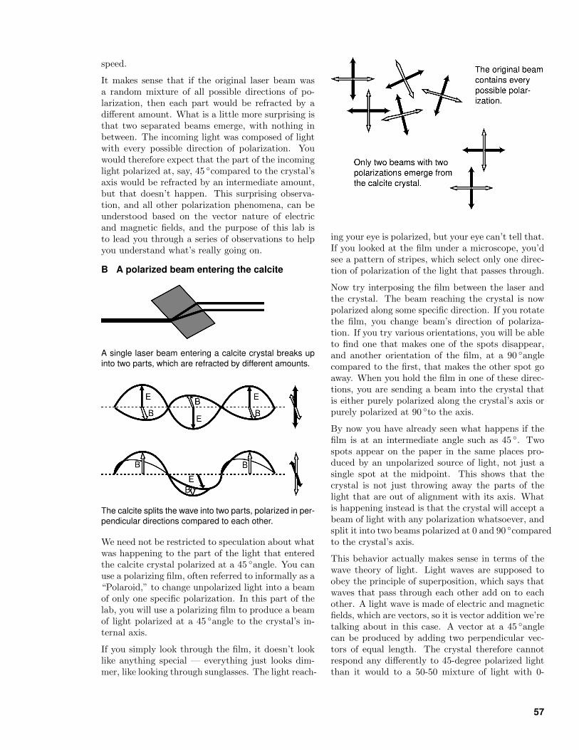
speed.

It makes sense that if the original laser beam wasa random mixture of all possible directions of po-larization, then each part would be refracted by adifferent amount. What is a little more surprising isthat two separated beams emerge, with nothing inbetween. The incoming light was composed of lightwith every possible direction of polarization. Youwould therefore expect that the part of the incominglight polarized at, say, 45 compared to the crystal’saxis would be refracted by an intermediate amount,but that doesn’t happen. This surprising observa-tion, and all other polarization phenomena, can beunderstood based on the vector nature of electricand magnetic fields, and the purpose of this lab isto lead you through a series of observations to helpyou understand what’s really going on.

B A polarized beam entering the calcite

A single laser beam entering a calcite crystal breaks upinto two parts, which are refracted by different amounts.

The calcite splits the wave into two parts, polarized in per-pendicular directions compared to each other.

We need not be restricted to speculation about whatwas happening to the part of the light that enteredthe calcite crystal polarized at a 45 angle. You canuse a polarizing film, often referred to informally as a“Polaroid,” to change unpolarized light into a beamof only one specific polarization. In this part of thelab, you will use a polarizing film to produce a beamof light polarized at a 45 angle to the crystal’s in-ternal axis.

If you simply look through the film, it doesn’t looklike anything special — everything just looks dim-mer, like looking through sunglasses. The light reach-

ing your eye is polarized, but your eye can’t tell that.If you looked at the film under a microscope, you’dsee a pattern of stripes, which select only one direc-tion of polarization of the light that passes through.

Now try interposing the film between the laser andthe crystal. The beam reaching the crystal is nowpolarized along some specific direction. If you rotatethe film, you change beam’s direction of polariza-tion. If you try various orientations, you will be ableto find one that makes one of the spots disappear,and another orientation of the film, at a 90 anglecompared to the first, that makes the other spot goaway. When you hold the film in one of these direc-tions, you are sending a beam into the crystal thatis either purely polarized along the crystal’s axis orpurely polarized at 90 to the axis.

By now you have already seen what happens if thefilm is at an intermediate angle such as 45 . Twospots appear on the paper in the same places pro-duced by an unpolarized source of light, not just asingle spot at the midpoint. This shows that thecrystal is not just throwing away the parts of thelight that are out of alignment with its axis. Whatis happening instead is that the crystal will accept abeam of light with any polarization whatsoever, andsplit it into two beams polarized at 0 and 90 comparedto the crystal’s axis.

This behavior actually makes sense in terms of thewave theory of light. Light waves are supposed toobey the principle of superposition, which says thatwaves that pass through each other add on to eachother. A light wave is made of electric and magneticfields, which are vectors, so it is vector addition we’retalking about in this case. A vector at a 45 anglecan be produced by adding two perpendicular vec-tors of equal length. The crystal therefore cannotrespond any differently to 45-degree polarized lightthan it would to a 50-50 mixture of light with 0-

57

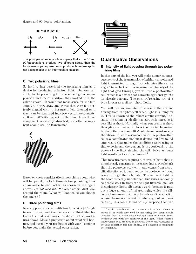
degree and 90-degree polarization.

The principle of superposition implies that if the 0 and90 polarizations produce two different spots, then thetwo waves superimposed must produce those two spots,not a single spot at an intermediate location.

C Two polarizing films

So far I’ve just described the polarizing film as adevice for producing polarized light. But one canapply to the polarizing film the same logic of super-position and vector addition that worked with thecalcite crystal. It would not make sense for the filmsimply to throw away any waves that were not per-fectly aligned with it, because a field oriented on aslant can be analyzed into two vector components,at 0 and 90 with respect to the film. Even if onecomponent is entirely absorbed, the other compo-nent should still be transmitted.

Based on these considerations, now think about whatwill happen if you look through two polarizing filmsat an angle to each other, as shown in the figureabove. Do not look into the laser beam! Just lookaround the room. What will happen as you changethe angle θ?

D Three polarizing films

Now suppose you start with two films at a 90 angleto each other, and then sandwich a third film be-tween them at a 45 angle, as shown in the two fig-ures above. Make a prediction about what will hap-pen, and discuss your prediction with your instructorbefore you make the actual observation.

Quantitative ObservationsE Intensity of light passing through two polar-

izing films

In this part of the lab, you will make numerical mea-surements of the transmission of initially unpolarizedlight transmitted through two polarizing films at anangle θ to each other. To measure the intensity of thelight that gets through, you will use a photovoltaiccell, which is a device that converts light energy intoan electric current. The ones we’re using are of atype known as a silicon photodiode.

You will use an ammeter to measure the currentflowing from the photocell when light is shining onit. This is known as the “short-circuit current,” be-cause the ammeter ideally has zero resistance, so itacts like a short. Normally when you create a shortthrough an ammeter, it blows the fuse in the meter,but here there is about 40 kΩ of internal resistance inthe silicon, which is a semiconductor. A photovoltaiccell is a complicated nonlinear device, but I’ve foundempirically that under the conditions we’re using inthis experiment, the current is proportional to thepower of the light striking the cell: twice as muchlight results in twice the current.1

This measurement requires a source of light that isunpolarized, constant in intensity, has a wavelengththat the polaroids work with, and comes from a spe-cific direction so it can’t get to the photocell withoutgoing through the polaroids. The ambient light inthe room is nearly unpolarized, but varies randomlyas people walk in front of the light fixtures, etc. Anincandescent lightbulb doesn’t work, because it putsout a huge amount of infrared light, which the sili-con cell measures but the polaroids can’t work with.A laser beam is constant in intensity, but as I wascreating this lab I found to my surprise that the

1It’s also possible to use the same cell with a voltmeteracross it, in which case we’d be measuring the “open-circuitvoltage;” but the open-circuit voltage varies in a much morenonlinear way with the intensity of the light. When rooftopphotovoltaic cells are used to generate power, the resistance ofthe load is neither zero nor infinity, and is chosen to maximizethe efficiency.

58 Lab 14 Polarization

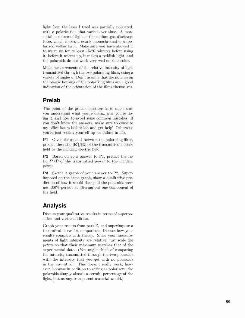
light from the laser I tried was partially polarized,with a polarization that varied over time. A moresuitable source of light is the sodium gas dischargetube, which makes a nearly monochromatic, unpo-larized yellow light. Make sure you have allowed itto warm up for at least 15-20 minutes before usingit; before it warms up, it makes a reddish light, andthe polaroids do not work very well on that color.

Make measurements of the relative intensity of lighttransmitted through the two polarizing films, using avariety of angles θ. Don’t assume that the notches onthe plastic housing of the polarizing films are a goodindication of the orientation of the films themselves.


P1 Given the angle θ between the polarizing films,predict the ratio |E′|/|E| of the transmitted electricfield to the incident electric field.

P2 Based on your answer to P1, predict the ra-tio P ′/P of the transmitted power to the incidentpower.

P3 Sketch a graph of your answer to P2. Super-imposed on the same graph, show a qualitative pre-diction of how it would change if the polaroids werenot 100% perfect at filtering out one component ofthe field.

AnalysisDiscuss your qualitative results in terms of superpo-sition and vector addition.

Graph your results from part E, and superimpose atheoretical curve for comparison. Discuss how yourresults compare with theory. Since your measure-ments of light intensity are relative, just scale thepoints so that their maximum matches that of theexperimental data. (You might think of comparingthe intensity transmitted through the two polaroidswith the intensity that you get with no polaroidsin the way at all. This doesn’t really work, how-ever, because in addition to acting as polarizers, thepolaroids simply absorb a certain percentage of thelight, just as any transparent material would.)

59

Appendix 1: Format of Lab Writeups

Lab reports must be three pages or less, not countingyour raw data. The format should be as follows:

Title

Raw data — Keep actual observations separate fromwhat you later did with them.These are the results of the measurements you takedown during the lab, hence they come first. Writeyour raw data directly in your lab book; don’t writethem on scratch paper and recopy them later. Don’tuse pencil. The point is to separate facts from opin-ions, observations from inferences.

Procedure — Did you have to create your ownmethods for getting some of the raw data?Do not copy down the procedure from the manual.In this section, you only need to explain any meth-ods you had to come up with on your own, or caseswhere the methods suggested in the handout didn’twork and you had to do something different. Don’twrite anything here unless you think I will really careand want to change how we do the lab in the future.In most cases this section can be totally blank. Donot discuss how you did your calculations here, justhow you got your raw data.

Abstract — What did you find out? Why is it im-portant?The “abstract” of a scientific paper is a short para-graph at the top that summarizes the experiment’sresults in a few sentences.

Many of our labs are comparisons of theory and ex-periment. The abstract for such a lab needs to saywhether you think the experiment was consistentwith theory, or not consistent with theory. If yourresults deviated from the ideal equations, don’t beafraid to say so. After all, this is real life, and manyof the equations we learn are only approximations,or are only valid in certain circumstances. However,(1) if you simply mess up, it is your responsibilityto realize it in lab and do it again, right; (2) youwill never get exact agreement with theory, becausemeasurements are not perfectly exact — the impor-tant issue is whether your results agree with theoryto roughly within the error bars.

The abstract is not a statement of what you hopedto find out. It’s a statement of what you did findout. It’s like the brief statement at the beginningof a debate: “The U.S. should have free trade withChina.” It’s not this: “In this debate, we will discuss

whether the U.S. should have free trade with China.”

If this is a lab that has just one important numericalresult (or maybe two or three of them), put themin your abstract, with error bars where appropriate.There should normally be no more than two to fournumbers here. Do not recapitulate your raw datahere — this is for your final results.

If you’re presenting a final result with error bars,make sure that the number of significant figures isconsistent with your error bars. For example, if youwrite a result as 323.54± 6 m/s, that’s wrong. Yourerror bars say that you could be off by 6 in the ones’place, so the 5 in the tenths’ place and the four inthe hundredths’ place are completely meaningless.

If you’re presenting a number in scientific notation,with error bars, don’t do it like this

1.234× 10−89 m/s± 3× 10−92 m/s ,

do it like this

(1.234± 0.003)× 10−89 m/s ,

so that we can see easily which digit of the result theerror bars apply to.

Calculations and Reasoning — Convince me ofwhat you claimed in your abstract.Often this section consists of nothing more than thecalculations that you started during lab. If those cal-culations are clear enough to understand, and thereis nothing else of interest to explain, then it is notnecessary to write up a separate narrative of youranalysis here. If you have a long series of similarcalculations, you may just show one as a sample. Ifyour prelab involved deriving equations that you willneed, repeat them here without the derivation.

In some labs, you will need to go into some detailhere by giving logical arguments to convince me thatthe statements you made in the abstract follow log-ically from your data. Continuing the debate meta-phor, if your abstract said the U.S. should have freetrade with China, this is the rest of the debate, whereyou convince me, based on data and logic, that weshould have free trade.

60 Lab Appendix 1: Format of Lab Writeups

61

Appendix 2: Basic Error Analysis

No measurement is perfectly ex-act.One of the most common misconceptions about sci-ence is that science is “exact.” It is always a strug-gle to get beginning science students to believe thatno measurement is perfectly correct. They tend tothink that if a measurement is a little off from the“true” result, it must be because of a mistake — ifa pro had done it, it would have been right on themark. Not true!

What scientists can do is to estimate just how faroff they might be. This type of estimate is calledan error bar, and is expressed with the ± symbol,read “plus or minus.” For instance, if I measure mydog’s weight to be 52 ± 2 pounds, I am saying thatmy best estimate of the weight is 52 pounds, and Ithink I could be off by roughly 2 pounds either way.The term “error bar” comes from the conventionalway of representing this range of uncertainty of ameasurement on a graph, but the term is also usedwhen no graph is involved.

Some very good scientific work results in measure-ments that nevertheless have large error bars. Forinstance, the best measurement of the age of the uni-verse is now 15±5 billion years. That may not seemlike wonderful precision, but the people who did themeasurement knew what they were doing. It’s justthat the only available techniques for determiningthe age of the universe are inherently poor.

Even when the techniques for measurement are veryprecise, there are still error bars. For instance, elec-trons act like little magnets, and the strength of avery weak magnet such as an individual electron iscustomarily measured in units called Bohr magne-tons. Even though the magnetic strength of an elec-tron is one of the most precisely measured quantitiesever, the best experimental value still has error bars:1.0011596524± 0.0000000002 Bohr magnetons.

There are several reasons why it is important in sci-entific work to come up with a numerical estimateof your error bars. If the point of your experimentis to test whether the result comes out as predictedby a theory, you know there will always be somedisagreement, even if the theory is absolutely right.You need to know whether the measurement is rea-sonably consistent with the theory, or whether thediscrepancy is too great to be explained by the lim-

itations of the measuring devices.

Another important reason for stating results with er-ror bars is that other people may use your measure-ment for purposes you could not have anticipated.If they are to use your result intelligently, they needto have some idea of how accurate it was.

Error bars are not absolute limits.Error bars are not absolute limits. The true valuemay lie outside the error bars. If I got a better scale Imight find that the dog’s weight is 51.3±0.1 pounds,inside my original error bars, but it’s also possiblethat the better result would be 48.7 ± 0.1 pounds.Since there’s always some chance of being off by asomewhat more than your error bars, or even a lotmore than your error bars, there is no point in be-ing extremely conservative in an effort to make ab-solutely sure the true value lies within your statedrange. When a scientist states a measurement witherror bars, she is not saying “If the true value isoutside this range, I deserve to be drummed out ofthe profession.” If that was the case, then every sci-entist would give ridiculously inflated error bars toavoid having her career ended by one fluke out ofhundreds of published results. What scientists arecommunicating to each other with error bars is atypical amount by which they might be off, not anupper limit.

The important thing is therefore to define error barsin a standard way, so that different people’s state-ments can be compared on the same footing. Byconvention, it is usually assumed that people esti-mate their error bars so that about two times out ofthree, their range will include the true value (or theresults of a later, more accurate measurement withan improved technique).

Random and systematic errors.Suppose you measure the length of a sofa with atape measure as well as you can, reading it off tothe nearest millimeter. If you repeat the measure-ment again, you will get a different answer. (Thisis assuming that you don’t allow yourself to be psy-chologically biased to repeat your previous answer,and that 1 mm is about the limit of how well youcan see.) If you kept on repeating the measurement,

62 Lab Appendix 2: Basic Error Analysis

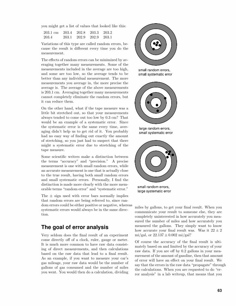
you might get a list of values that looked like this:

203.1 cm 203.4 202.8 203.3 203.2203.4 203.1 202.9 202.9 203.1

Variations of this type are called random errors, be-cause the result is different every time you do themeasurement.

The effects of random errors can be minimized by av-eraging together many measurements. Some of themeasurements included in the average are too high,and some are too low, so the average tends to bebetter than any individual measurement. The moremeasurements you average in, the more precise theaverage is. The average of the above measurementsis 203.1 cm. Averaging together many measurementscannot completely eliminate the random errors, butit can reduce them.

On the other hand, what if the tape measure was alittle bit stretched out, so that your measurementsalways tended to come out too low by 0.3 cm? Thatwould be an example of a systematic error. Sincethe systematic error is the same every time, aver-aging didn’t help us to get rid of it. You probablyhad no easy way of finding out exactly the amountof stretching, so you just had to suspect that theremight a systematic error due to stretching of thetape measure.

Some scientific writers make a distinction betweenthe terms “accuracy” and “precision.” A precisemeasurement is one with small random errors, whilean accurate measurement is one that is actually closeto the true result, having both small random errorsand small systematic errors. Personally, I find thedistinction is made more clearly with the more mem-orable terms “random error” and “systematic error.”

The ± sign used with error bars normally impliesthat random errors are being referred to, since ran-dom errors could be either positive or negative, whereassystematic errors would always be in the same direc-tion.

The goal of error analysisVery seldom does the final result of an experimentcome directly off of a clock, ruler, gauge or meter.It is much more common to have raw data consist-ing of direct measurements, and then calculationsbased on the raw data that lead to a final result.As an example, if you want to measure your car’sgas mileage, your raw data would be the number ofgallons of gas consumed and the number of milesyou went. You would then do a calculation, dividing

miles by gallons, to get your final result. When youcommunicate your result to someone else, they arecompletely uninterested in how accurately you mea-sured the number of miles and how accurately youmeasured the gallons. They simply want to knowhow accurate your final result was. Was it 22 ± 2mi/gal, or 22.137± 0.002 mi/gal?

Of course the accuracy of the final result is ulti-mately based on and limited by the accuracy of yourraw data. If you are off by 0.2 gallons in your mea-surement of the amount of gasoline, then that amountof error will have an effect on your final result. Wesay that the errors in the raw data “propagate” throughthe calculations. When you are requested to do “er-ror analysis” in a lab writeup, that means that you

63

are to use the techniques explained below to deter-mine the error bars on your final result. There aretwo sets of techniques you’ll need to learn:

techniques for finding the accuracy of your rawdata

techniques for using the error bars on your rawdata to infer error bars on your final result

Estimating random errors in rawdataWe now examine three possible techniques for es-timating random errors in your original measure-ments, illustrating them with the measurement ofthe length of the sofa.

Method #1: Guess

If you’re measuring the length of the sofa with ametric tape measure, then you can probably make areasonable guess as to the precision of your measure-ments. Since the smallest division on the tape mea-sure is one millimeter, and one millimeter is also nearthe limit of your ability to see, you know you won’tbe doing better than ± 1 mm, or 0.1 cm. Making al-lowances for errors in getting tape measure straightand so on, we might estimate our random errors tobe a couple of millimeters.

Guessing is fine sometimes, but there are at least twoways that it can get you in trouble. One is that stu-dents sometimes have too much faith in a measuringdevice just because it looks fancy. They think thata digital balance must be perfectly accurate, sinceunlike a low-tech balance with sliding weights on it,it comes up with its result without any involvementby the user. That is incorrect. No measurement isperfectly accurate, and if the digital balance onlydisplays an answer that goes down to tenths of agram, then there is no way the random errors areany smaller than about a tenth of a gram.

Another way to mess up is to try to guess the errorbars on a piece of raw data when you really don’thave enough information to make an intelligent esti-mate. For instance, if you are measuring the rangeof a rifle, you might shoot it and measure how farthe bullet went to the nearest centimeter, conclud-ing that your random errors were only ±1 cm. Inreality, however, its range might vary randomly byfifty meters, depending on all kinds of random fac-tors you don’t know about. In this type of situation,you’re better off using some other method of esti-mating your random errors.

Method #2: Repeated Measurements and the Two-Thirds Rule

If you take repeated measurements of the same thing,then the amount of variation among the numbers cantell you how big the random errors were. This ap-proach has an advantage over guessing your randomerrors, since it automatically takes into account allthe sources of random error, even ones you didn’tknow were present.

Roughly speaking, the measurements of the lengthof the sofa were mostly within a few mm of the av-erage, so that’s about how big the random errorswere. But let’s make sure we are stating our errorbars according to the convention that the true resultwill fall within our range of errors about two timesout of three. Of course we don’t know the “true”result, but if we sort out our list of measurementsin order, we can get a pretty reasonable estimate ofour error bars by taking half the range covered bythe middle two thirds of the list. Sorting out our listof ten measurements of the sofa, we have

202.8 cm 202.9 202.9 203.1 203.1203.1 203.2 203.3 203.4 203.4

Two thirds of ten is about 6, and the range coveredby the middle six measurements is 203.3 cm - 202.9cm, or 0.4 cm. Half that is 0.2 cm, so we’d esti-mate our error bars as ±0.2 cm. The average of themeasurements is 203.1 cm, so your result would bestated as 203.1± 0.2 cm.

One common mistake when estimating random er-rors by repeated measurements is to round off allyour measurements so that they all come out thesame, and then conclude that the error bars werezero. For instance, if we’d done some overenthu-siastic rounding of our measurements on the sofa,rounding them all off to the nearest cm, every singlenumber on the list would have been 203 cm. Thatwouldn’t mean that our random errors were zero!The same can happen with digital instruments thatautomatically round off for you. A digital balancemight give results rounded off to the nearest tenth ofa gram, and you may find that by putting the sameobject on the balance again and again, you alwaysget the same answer. That doesn’t mean it’s per-fectly precise. Its precision is no better than about±0.1 g.

Method #3: Repeated Measurements and the Stan-dard Deviation

The most widely accepted method for measuring er-ror bars is called the standard deviation. Here’s howthe method works, using the sofa example again.


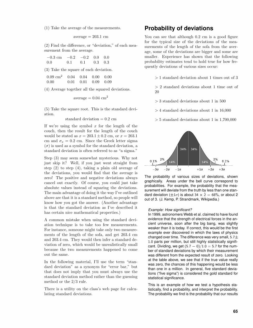
(1) Take the average of the measurements.

average = 203.1 cm

(2) Find the difference, or “deviation,” of each mea-surement from the average.

−0.3 cm −0.2 −0.2 0.0 0.00.0 0.1 0.1 0.3 0.3

(3) Take the square of each deviation.

0.09 cm2 0.04 0.04 0.00 0.000.00 0.01 0.01 0.09 0.09

(4) Average together all the squared deviations.

average = 0.04 cm2

(5) Take the square root. This is the standard devi-ation.

standard deviation = 0.2 cm

If we’re using the symbol x for the length of thecouch, then the result for the length of the couchwould be stated as x = 203.1± 0.2 cm, or x = 203.1cm and σx = 0.2 cm. Since the Greek letter sigma(σ) is used as a symbol for the standard deviation, astandard deviation is often referred to as “a sigma.”

Step (3) may seem somewhat mysterious. Why notjust skip it? Well, if you just went straight fromstep (2) to step (4), taking a plain old average ofthe deviations, you would find that the average iszero! The positive and negative deviations alwayscancel out exactly. Of course, you could just takeabsolute values instead of squaring the deviations.The main advantage of doing it the way I’ve outlinedabove are that it is a standard method, so people willknow how you got the answer. (Another advantageis that the standard deviation as I’ve described ithas certain nice mathematical properties.)

A common mistake when using the standard devi-ation technique is to take too few measurements.For instance, someone might take only two measure-ments of the length of the sofa, and get 203.4 cmand 203.4 cm. They would then infer a standard de-viation of zero, which would be unrealistically smallbecause the two measurements happened to comeout the same.

In the following material, I’ll use the term “stan-dard deviation” as a synonym for “error bar,” butthat does not imply that you must always use thestandard deviation method rather than the guessingmethod or the 2/3 rule.

There is a utility on the class’s web page for calcu-lating standard deviations.

Probability of deviationsYou can see that although 0.2 cm is a good figurefor the typical size of the deviations of the mea-surements of the length of the sofa from the aver-age, some of the deviations are bigger and some aresmaller. Experience has shown that the followingprobability estimates tend to hold true for how fre-quently deviations of various sizes occur:

> 1 standard deviation about 1 times out of 3

> 2 standard deviations about 1 time out of20

> 3 standard deviations about 1 in 500

> 4 standard deviations about 1 in 16,000

> 5 standard deviations about 1 in 1,700,000

The probability of various sizes of deviations, showngraphically. Areas under the bell curve correspond toprobabilities. For example, the probability that the mea-surement will deviate from the truth by less than one stan-dard deviation (±1σ) is about 34 × 2 = 68%, or about 2out of 3. (J. Kemp, P. Strandmark, Wikipedia.)

Example: How significant?In 1999, astronomers Webb et al. claimed to have foundevidence that the strength of electrical forces in the an-cient universe, soon after the big bang, was slightlyweaker than it is today. If correct, this would be the firstexample ever discovered in which the laws of physicschanged over time. The difference was very small, 5.7±1.0 parts per million, but still highly statistically signifi-cant. Dividing, we get (5.7− 0)/1.0 = 5.7 for the num-ber of standard deviations by which their measurementwas different from the expected result of zero. Lookingat the table above, we see that if the true value reallywas zero, the chances of this happening would be lessthan one in a million. In general, five standard devia-tions (“five sigma”) is considered the gold standard forstatistical significance.

This is an example of how we test a hypothesis sta-tistically, find a probability, and interpret the probability.The probability we find is the probability that our results

65

would differ this much from the hypothesis, if the hy-pothesis was true. It’s not the probability that the hy-pothesis is true or false, nor is it the probability that ourexperiment is right or wrong.

However, there is a twist to this story that shows howstatistics always have to be taken with a grain of salt. In2004, Chand et al. redid the measurement by a moreprecise technique, and found that the change was 0.6±0.6 parts per million. This is only one standard devia-tion away from the expected value of 0, which should beinterpreted as being statistically consistent with zero. Ifyou measure something, and you think you know whatthe result is supposed to be theoretically, then one stan-dard deviation is the amount you typically expect to beoff by — that’s why it’s called the “standard” deviation.Moreover, the Chand result is wildly statistically incon-sistent with the Webb result (see the example on page69), which means that one experiment or the other isa mistake. Most likely Webb at al. underestimated theirrandom errors, or perhaps there were systematic errorsin their experiment that they didn’t realize were there.

Precision of an averageWe decided that the standard deviation of our mea-surements of the length of the couch was 0.2 cm,i.e., the precision of each individual measurementwas about 0.2 cm. But I told you that the average,203.1 cm, was more precise than any individual mea-surement. How precise is the average? The answeris that the standard deviation of the average equals

standard deviation of one measurement√number of measurements

.

(An example on page 68 gives the reasoning thatleads to the square root.) That means that you cantheoretically measure anything to any desired preci-sion, simply by averaging together enough measure-ments. In reality, no matter how small you makeyour random error, you can’t get rid of systematic er-rors by averaging, so after a while it becomes point-less to take any more measurements.


67

Appendix 3: Propagation of Errors

Propagation of the error from asingle variableIn the previous appendix we looked at techniquesfor estimating the random errors of raw data, butnow we need to know how to evaluate the effects ofthose random errors on a final result calculated fromthe raw data. For instance, suppose you are given acube made of some unknown material, and you areasked to determine its density. Density is definedas ρ = m/v (ρ is the Greek letter “rho”), and thevolume of a cube with edges of length b is v = b3, sothe formula

ρ = m/b3

will give you the density if you measure the cube’smass and the length of its sides. Suppose you mea-sure the mass very accurately as m = 1.658±0.003 g,but you know b = 0.85±0.06 cm with only two digitsof precision. Your best value for ρ is 1.658 g/(0.85 cm)3 =2.7 g/cm3.

How can you figure out how precise this value for ρis? We’ve already made sure not to keep more thantwosignificant figures for ρ, since the less accuratepiece of raw data had only two significant figures.We expect the last significant figure to be somewhatuncertain, but we don’t yet know how uncertain. Asimple method for this type of situation is simply tochange the raw data by one sigma, recalculate theresult, and see how much of a change occurred. Inthis example, we add 0.06 cm to b for comparison.

b = 0.85 cm gave ρ = 2.7 g/cm3

b = 0.91 cm gives ρ = 2.2 g/cm3

The resulting change in the density was 0.5 g/cm3,so that is our estimate for how much it could havebeen off by:

ρ = 2.7± 0.5 g/cm3 .

Propagation of the error from sev-eral variablesWhat about the more general case in which no onepiece of raw data is clearly the main source of error?For instance, suppose we get a more accurate mea-surement of the edge of the cube, b = 0.851± 0.001cm. In percentage terms, the accuracies of m and

b are roughly comparable, so both can cause sig-nificant errors in the density. The following moregeneral method can be applied in such cases:

(1) Change one of the raw measurements, say m, byone standard deviation, and see by how much thefinal result, ρ, changes. Use the symbol Qm for theabsolute value of that change.

m = 1.658 g gave ρ = 2.690 g/cm3

m = 1.661 g gives ρ = 2.695 g/cm3

Qm = change in ρ = 0.005 g/cm3

(2) Repeat step (1) for the other raw measurements.

b = 0.851 cm gave ρ = 2.690 g/cm3

b = 0.852 cm gives ρ = 2.681 g/cm3

Qb = change in ρ = 0.009 g/cm3

(3) The error bars on ρ are given by the formula

σρ =√Q2m +Q2

b ,

yielding σρ = 0.01 g/cm3. Intuitively, the idea hereis that if our result could be off by an amount Qmbecause of an error in m, and by Qb because of b,then if the two errors were in the same direction, wemight by off by roughly |Qm| + |Qb|. However, it’sequally likely that the two errors would be in oppo-site directions, and at least partially cancel. The ex-pression

√Q2m +Q2

b gives an answer that’s smallerthan Qm+Qb, representing the fact that the cancel-lation might happen.

The final result is ρ = 2.69± 0.01 g/cm3.

Example: An averageOn page 66 I claimed that averaging a bunch of mea-surements reduces the error bars by the square root ofthe number of measurements. We can now see thatthis is a special case of propagation of errors.

For example, suppose Alice measures the circumfer-ence c of a guinea pig’s waist to be 10 cm, Using theguess method, she estimates that her error bars areabout ±1 cm (worse than the normal normal ∼ 1 mmerror bars for a tape measure, because the guinea pigwas squirming). Bob then measures the same thing,and gets 12 cm. The average is computed as

c =A + B

2,

where A is Alice’s measurement, and B is Bob’s, giving11 cm. If Alice had been off by one standard devia-tion (1 cm), it would have changed the average by 0.5

68 Lab Appendix 3: Propagation of Errors

cm, so we have QA = 0.5 cm, and likewise QB = 0.5cm. Combining these, we find σc =

√Q2

A + Q2B = 0.7

cm, which is simply (1.0 cm)/√2. The final result is

c = (11.0 ± 0.7) cm. (This violates the usual rule forsignificant figures, which is that the final result shouldhave no more sig figs than the least precise piece ofdata that went into the calculation. That’s okay, be-cause the sig fig rules are just a quick and dirty wayof doing propagation of errors. We’ve done real propa-gation of errors in this example, and it turns out that theerror is in the first decimal place, so the 0 in that placeis entitled to hold its head high as a real sig fig, albeit arelatively imprecise one with an uncertainty of ±7.)

Example: The difference between two measurementsIn the example on page 65, we saw that two groupsof scientists measured the same thing, and the resultswere W = 5.7± 1.0 for Webb et al. and C = 0.6± 0.6for Chand et al. It’s of interest to know whether thedifference between their two results is small enough tobe explained by random errors, or so big that it couldn’tpossibly have happened by chance, indicating that some-one messed up. The figure shows each group’s results,with error bars, on the number line. We see that the twosets of error bars don’t overlap with one another, but er-ror bars are not absolute limits, so it’s perfectly possibleto have non-overlapping error bars by chance, but thegap between the error bars is very large compared tothe error bars themselves, so it looks implausible thatthe results could be statistically consistent with one an-other. I’ve tried to suggest this visually with the shadingunderneath the data-points.

To get a sharper statistical test, we can calculate thedifference d between the two results,

d = W − C ,

which is 5.1. Since the operation is simply the subtrac-tion of the two numbers, an error in either input justcauses an error in the output that is of the same size.Therefore we have QW = 1.0 and QC = 0.6, resultingin σd =

√Q2

W + Q2C = 1.2. We find that the difference

between the two results is d = 5.1± 1.2, which differsfrom zero by 5.1/1.2 ≈ 4 standard deviations. Lookingat the table on page 65, we see that the chances thatd would be this big by chance are extremely small, lessthan about one in ten thousand. We can conclude to ahigh level of statistical confidence that the two groups’measurements are inconsistent with one another, andthat one group is simply wrong.

69

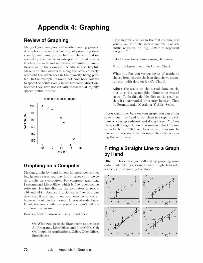
Appendix 4: Graphing

Review of GraphingMany of your analyses will involve making graphs.A graph can be an efficient way of presenting datavisually, assuming you include all the informationneeded by the reader to interpret it. That meanslabeling the axes and indicating the units in paren-theses, as in the example. A title is also helpful.Make sure that distances along the axes correctlyrepresent the differences in the quantity being plot-ted. In the example, it would not have been correctto space the points evenly in the horizontal direction,because they were not actually measured at equallyspaced points in time.

Graphing on a ComputerMaking graphs by hand in your lab notebook is fine,but in some cases you may find it saves you time todo graphs on a computer. For computer graphing,I recommend LibreOffice, which is free, open-sourcesoftware. It’s installed on the computers in rooms416 and 418. Because LibreOffice is free, you candownload it and put it on your own computer athome without paying money. If you already knowExcel, it’s very similar — you almost can’t tell it’sa different program.

Here’s a brief rundown on using LibreOffice:

On Windows, go to the Start menu and chooseAll Programs, LibreOffice, and LibreOffice Calc.On Linux, do Applications, Office, OpenOffice,Spreadsheet.

Type in your x values in the first column, andyour y values in the second column. For sci-entific notation, do, e.g., 5.2e-7 to represent5.2× 10−7.

Select those two columns using the mouse.

From the Insert menu, do Object:Chart.

When it offers you various styles of graphs tochoose from, choose the icon that shows a scat-ter plot, with dots on it (XY Chart).

Adjust the scales so the actual data on theplot is as big as possible, eliminating wastedspace. To do this, double-click on the graph sothat it’s surrounded by a gray border. Thendo Format, Axis, X Axis or Y Axis, Scale.

If you want error bars on your graph you can eitherdraw them in by hand or put them in a separate col-umn of your spreadsheet and doing Insert, Y ErrorBars, Cell Range. Under Parameters, check “Samevalue for both.” Click on the icon, and then use themouse in the spreadsheet to select the cells contain-ing the error bars.

Fitting a Straight Line to a Graphby HandOften in this course you will end up graphing somedata points, fitting a straight line through them witha ruler, and extracting the slope.

70 Lab Appendix 4: Graphing

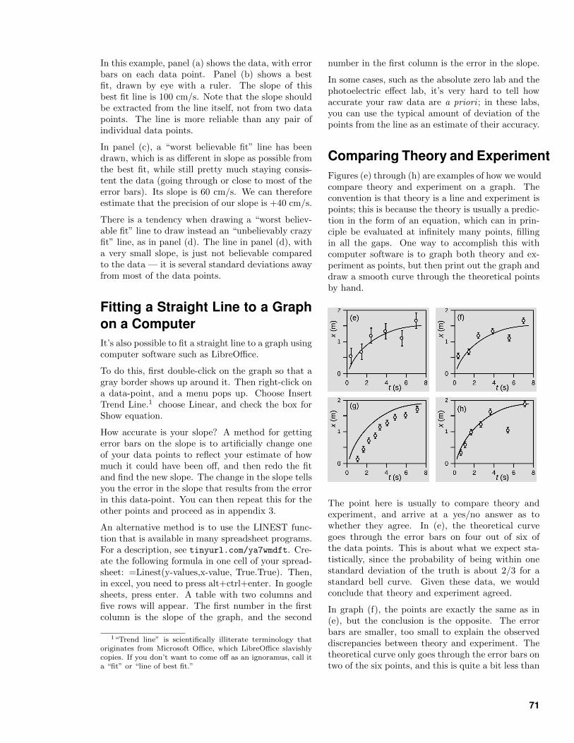
In this example, panel (a) shows the data, with errorbars on each data point. Panel (b) shows a bestfit, drawn by eye with a ruler. The slope of thisbest fit line is 100 cm/s. Note that the slope shouldbe extracted from the line itself, not from two datapoints. The line is more reliable than any pair ofindividual data points.

In panel (c), a “worst believable fit” line has beendrawn, which is as different in slope as possible fromthe best fit, while still pretty much staying consis-tent the data (going through or close to most of theerror bars). Its slope is 60 cm/s. We can thereforeestimate that the precision of our slope is +40 cm/s.

There is a tendency when drawing a “worst believ-able fit” line to draw instead an “unbelievably crazyfit” line, as in panel (d). The line in panel (d), witha very small slope, is just not believable comparedto the data — it is several standard deviations awayfrom most of the data points.

Fitting a Straight Line to a Graphon a ComputerIt’s also possible to fit a straight line to a graph usingcomputer software such as LibreOffice.

To do this, first double-click on the graph so that agray border shows up around it. Then right-click ona data-point, and a menu pops up. Choose InsertTrend Line.1 choose Linear, and check the box forShow equation.

How accurate is your slope? A method for gettingerror bars on the slope is to artificially change oneof your data points to reflect your estimate of howmuch it could have been off, and then redo the fitand find the new slope. The change in the slope tellsyou the error in the slope that results from the errorin this data-point. You can then repeat this for theother points and proceed as in appendix 3.

An alternative method is to use the LINEST func-tion that is available in many spreadsheet programs.For a description, see tinyurl.com/ya7wmdft. Cre-ate the following formula in one cell of your spread-sheet: =Linest(y-values,x-value, True.True). Then,in excel, you need to press alt+ctrl+enter. In googlesheets, press enter. A table with two columns andfive rows will appear. The first number in the firstcolumn is the slope of the graph, and the second

1“Trend line” is scientifically illiterate terminology thatoriginates from Microsoft Office, which LibreOffice slavishlycopies. If you don’t want to come off as an ignoramus, call ita “fit” or “line of best fit.”

number in the first column is the error in the slope.

In some cases, such as the absolute zero lab and thephotoelectric effect lab, it’s very hard to tell howaccurate your raw data are a priori ; in these labs,you can use the typical amount of deviation of thepoints from the line as an estimate of their accuracy.

Comparing Theory and ExperimentFigures (e) through (h) are examples of how we wouldcompare theory and experiment on a graph. Theconvention is that theory is a line and experiment ispoints; this is because the theory is usually a predic-tion in the form of an equation, which can in prin-ciple be evaluated at infinitely many points, fillingin all the gaps. One way to accomplish this withcomputer software is to graph both theory and ex-periment as points, but then print out the graph anddraw a smooth curve through the theoretical pointsby hand.

The point here is usually to compare theory andexperiment, and arrive at a yes/no answer as towhether they agree. In (e), the theoretical curvegoes through the error bars on four out of six ofthe data points. This is about what we expect sta-tistically, since the probability of being within onestandard deviation of the truth is about 2/3 for astandard bell curve. Given these data, we wouldconclude that theory and experiment agreed.

In graph (f), the points are exactly the same as in(e), but the conclusion is the opposite. The errorbars are smaller, too small to explain the observeddiscrepancies between theory and experiment. Thetheoretical curve only goes through the error bars ontwo of the six points, and this is quite a bit less than

71

we would expect statistically.

Graph (g) also shows disagreement between theoryand experiment, but now we have a clear systematicerror. In (h), the fifth data point looks like a mistake.Ideally you would notice during lab that somethinghad gone wrong, and go back and check whether youcould reproduce the result.

72 Lab Appendix 4: Graphing

73

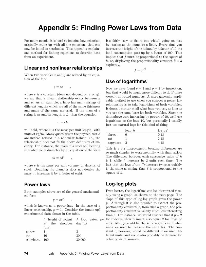
Appendix 5: Finding Power Laws from Data

For many people, it is hard to imagine how scientistsoriginally came up with all the equations that cannow be found in textbooks. This appendix explainsone method for finding equations to describe datafrom an experiment.

Linear and nonlinear relationshipsWhen two variables x and y are related by an equa-tion of the form

y = cx ,

where c is a constant (does not depend on x or y),we say that a linear relationship exists between xand y. As an example, a harp has many strings ofdifferent lengths which are all of the same thicknessand made of the same material. If the mass of astring is m and its length is L, then the equation

m = cL

will hold, where c is the mass per unit length, withunits of kg/m. Many quantities in the physical worldare instead related in a nonlinear fashion, i.e., therelationship does not fit the above definition of lin-earity. For instance, the mass of a steel ball bearingis related to its diameter by an equation of the form

m = cd3 ,

where c is the mass per unit volume, or density, ofsteel. Doubling the diameter does not double themass, it increases it by a factor of eight.

Power lawsBoth examples above are of the general mathemati-cal form

y = cxp ,

which is known as a power law. In the case of alinear relationship, p = 1. Consider the (made-up)experimental data shown in the table.

h=height of rodentat the shoulder(cm)

f=food eaten perday (g)

shrew 1 3rat 10 300capybara 100 30,000

It’s fairly easy to figure out what’s going on justby staring at the numbers a little. Every time youincrease the height of the animal by a factor of 10, itsfood consumption goes up by a factor of 100. Thisimplies that f must be proportional to the square ofh, or, displaying the proportionality constant k = 3explicitly,

f = 3h2 .

Use of logarithmsNow we have found c = 3 and p = 2 by inspection,but that would be much more difficult to do if theseweren’t all round numbers. A more generally appli-cable method to use when you suspect a power-lawrelationship is to take logarithms of both variables.It doesn’t matter at all what base you use, as long asyou use the same base for both variables. Since thedata above were increasing by powers of 10, we’ll uselogarithms to the base 10, but personally I usuallyjust use natural logs for this kind of thing.

log10 h log10 fshrew 0 0.48rat 1 2.48capybara 2 4.48

This is a big improvement, because differences areso much simpler to work mentally with than ratios.The difference between each successive value of his 1, while f increases by 2 units each time. Thefact that the logs of the f ′s increase twice as quicklyis the same as saying that f is proportional to thesquare of h.

Log-log plotsEven better, the logarithms can be interpreted visu-ally using a graph, as shown on the next page. Theslope of this type of log-log graph gives the powerp. Although it is also possible to extract the pro-portionality constant, c, from such a graph, the pro-portionality constant is usually much less interestingthan p. For instance, we would suspect that if p = 2for rodents, then it might also equal 2 for frogs orants. Also, p would be the same regardless of whatunits we used to measure the variables. The con-stant c, however, would be different if we used dif-ferent units, and would also probably be different forother types of animals.

74 Lab Appendix 5: Finding Power Laws from Data

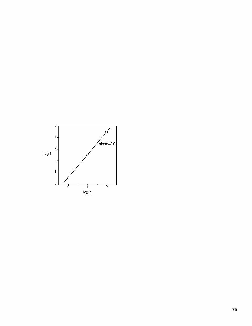
75

Appendix 6: Using a Multimeter

The most convenient instrument for measuring cur-rents and voltage differences is called a digital mul-timeter (DMM), or simply a multimeter. “Digital”means that it shows the thing being measured on acalculator-style LCD display. “Multimeter” meansthat it can measure current, voltage, or resistance,depending on how you have it set up. Since we havemany different types of multimeters, these instruc-tions only cover the standard rules and methods thatapply to all such meters. You may need to check withyour instructor regarding a few of the particulars forthe meter you have available.

Measuring currentWhen using a meter to measure current, the metermust be in series with the circuit, so that every elec-tron going by is forced to go through the meter andcontribute to a current in the meter. Many multime-ters have more than one scale for measuring a giventhing. For instance, a meter may have a milliampscale and an amp scale. One is used for measuringsmall currents and the other for large currents. Youmay not be sure in advance what scale is appropri-ate, but that’s not big problem — once everythingis hooked up, you can try different scales and seewhat’s appropriate. Use the switch or buttons on thefront to select one of the current scales. The connec-tions to the meter should be made at the “common”socket (“COM”) and at the socket labeled “A” forAmperes.

Measuring voltageFor a voltage measurement, use the switch or but-tons on the front to select one of the voltage scales.(If you forget, and hook up the meter while theswitch is still on a current scale, you may blow afuse.) You always measure voltage differences witha meter. One wire connects the meter to one pointin the circuit, and the other connects the meter toanother point in a circuit. The meter measures thedifference in voltage between those two points. Forexample, to measure the voltage across a resistor,you must put the meter in parallel with the resis-tor. The connections to the meter should be madeat the “common” socket (“COM”) and at the socketlabeled “V” for Volts.

Blowing a fuse is not a big deal.If you hook up your multimeter incorrectly, it is pos-sible to blow a fuse inside. This is especially likely tohappen if you set up the meter to measure current(meaning it has a small internal resistance) but hookit up in parallel with a resistor, creating a large volt-age difference across it. Blowing a fuse is not a bigproblem, but it can be frustrating if you don’t real-ize what’s happened. If your meter suddenly stopsworking, you should check the fuse.

76 Lab Appendix 6: Using a Multimeter

77

Appendix 7: High Voltage Safety Checklist

Name:

Never work with high voltages by yourself.

Do not leave HV wires exposed - make surethere is insulation.

Turn the high-voltage supply off while workingon the circuit.

When the voltage is on, avoid using both handsat once to touch the apparatus. Keep one hand inyour pocket while using the other to touch the ap-paratus. That way, it is unlikely that you will get ashock across your chest.

It is possible for an electric current to causeyour hand to clench involuntarily. If you observe thishappening to your partner, do not try to pry theirhand away, because you could become incapacitatedas well — simply turn off the switch or pull the plugout of the wall.

78 Lab Appendix 7: High Voltage Safety Checklist

79

Appendix ??: Comment Codes forLab Writeups

A. Generala1. Don’t write numbers without units.(25% off)a2. If something is wrong, cross it out.Don’t make me guess which version tograde.a3. Your writeup is too long. The lengthlimit is 3 pages, not including raw data.a4. If your writeup includes printouts, sta-ple them in sideways with a single staple.a5. See appendix 1 for the format of labwriteups.a6. Don’t state speculation as a firm con-clusion.a7. Leave more space for me to write com-ments.a8. Cut unnecessary words. Use activevoice. Write in a simple, direct style.a9. Don’t write walls of text. Use para-graph breaks.a10. Cut any sentence that doesn’t carryinformation.a11. This paragraph needs a topic sentence.a12. Express this as an equation.a13. Don’t present details unless you’vealready made it clear why we would care.Don’t write slavishly in chronological order.a14. The first sentence of any piece of writ-ing must make an implicit promise that theremainder will interest the reader.B. Raw datab1. Don’t mix raw data with calculations.(25% off)b2. Write raw data in pen, directly in thenotebook.b3. This isn’t raw data. This is a summaryor copy.C. Procedurec1. Don’t repeat the lab manual.c2. Don’t write anything about your proce-dure unless it’s something truly original thatyou think I would be interested in knowingabout, or I wouldn’t be able to understandyour writeup without it.D. Abstract – see appendix 1

d1. Your abstract is too long.d2. Don’t recap raw data in your abstract.d3. Don’t describe calculations in your ab-stract.d4. The only numbers that should be inyour abstract are important final resultsthat support your conclusion or that consti-tute the purpose of the lab.d5. Your abstract needs to include numeri-cal results that support your conclusions.d6. Give error bars in your abstract.d7. Where is your abstract?d8. Your abstract is for results. This isn’ta result of your experiment.d9. This isn’t important enough to go inyour abstract.d10. What was the point of the lab, andwhy would anyone care?d11. Don’t just give results. Interpret them.d12. We knew this before you did the lab.d13. This lab was a quantitative test. Re-stating it qualitatively isn’t interesting.d14. This lab is a comparison of theory andexperiment. Did they agree, or not?d15. Your results don’t support your con-clusions. Write about what really hap-pened, not what you wanted to happen.d16. One observation can never prove ageneral rule.E. Error analysis – see appendices 2and 3e1. A standard deviation only measureserror if it comes from numbers that weresupposed to be the same, e.g., repeatedmeasurements of the same thing.e2. In propagation of errors, don’t do bothhigh and low. See appendix 3.e3. In propagation of errors, only changeone variable at a time. See appendix 3.e4. Don’t round severely when calculat-ing Q’s. Your Q’s are just measuring yourrounding errors.e5. A Q is the amount by which the outputof the calculation changes, not its inputs.e6. A Q is a change in the result, not the

82 Lab Appendix ??: Comment Codes for Lab Writeups

result itself.e7. Use your error bars in forming yourconclusions. Otherwise what was the pointof calculating them?e8. Give a probabilistic interpretation, asin the examples at the end of appendix 2.e9. You’re interpreting this probability in-correctly. It’s the probability that yourresults would have differed this much fromthe hypothesis, if the hypothesis were true.e10. % errors are useless. Teachers haveyou do them if you don’t know about realerror analysis.e11. If random errors are included in yourpropagation of errors, listing them here ver-bally is pointless.e12. Don’t speculate about systematic er-rors without investigating them. Estimatetheir possible size. Would they produce aneffect in the right direction?G. Graphing – see appendix 4g1. Label the axes to show what variablesare being graphed and what their units are,e.g., x (km).g2. Your graph should be bigger.g3. If graphing by hand, do it on graphpaper.g4. Choose an appropriate scale for yourgraph, so that the data are not squisheddown. Don’t just accept the default fromthe software if it’s wrong. See app. 4 forhow to do this using Libre Office.g5. “Dot to dot” style is wrong in a scien-

tific graph.g6. The independent variable (the one youcontrol directly) goes on the x axis, and thedependent variable on the y. Or: cause onx, effect on y.g7. On a scientific graph, use dots to showdata, a line or curve for theory or a fit tothe data.g8. “Trend line” is scientifically illiterate.It’s called a line of best fit.S. Calculations and sig figss1. Think about the sizes of numbers andwhether they make sense. This numberdoesn’t make sense.s2. Where did this number come from?s3. This number has too many sig figs (e.g.,more than the number of sig figs in the rawdata).s4. Don’t round off severely for sig figs atintermediate steps. Rounding errors can ac-cumulate.s5. You’re wasting your time by writingdown many non-significant figures.s6. Your result has too many sig figs. Theerror bars show that you don’t have thismuch precision.s7. The Calculations and Reasoning sec-tion usually just consists of the calculationsyou’ve already written.You don’t need towrite a separate narrative.s8. Put your calculator in scientific notationmode.

Appendix 10: The Open PublicationLicense

Copyright (c) 1999-2001 B. Crowell and V. Roundy. All rights reserved.

These materials are open-content licensed under the OPL 1.0 license. A copy of the licenseis given below, and the original is available at http://opencontent.org.

LICENSE

Terms and Conditions for Copying, Distributing, and Modifying

Items other than copying, distributing, and modifying the Content with which this licensewas distributed (such as using, etc.) are outside the scope of this license.

1. You may copy and distribute exact replicas of the OpenContent (OC) as you receive it,in any medium, provided that you conspicuously and appropriately publish on each copyan appropriate copyright notice and disclaimer of warranty; keep intact all the notices thatrefer to this License and to the absence of any warranty; and give any other recipients ofthe OC a copy of this License along with the OC. You may at your option charge a fee forthe media and/or handling involved in creating a unique copy of the OC for use offline, youmay at your option offer instructional support for the OC in exchange for a fee, or you mayat your option offer warranty in exchange for a fee. You may not charge a fee for the OCitself. You may not charge a fee for the sole service of providing access to and/or use of theOC via a network (e.g., the Internet), whether it be via the world wide web, FTP, or anyother method.

2. You may modify your copy or copies of the OpenContent or any portion of it, thusforming works based on the Content, and distribute such modifications or work under theterms of Section 1 above, provided that you also meet all of these conditions:

a) You must cause the modified content to carry prominent notices stating that you changedit, the exact nature and content of the changes, and the date of any change.

b) You must cause any work that you distribute or publish, that in whole or in part containsor is derived from the OC or any part thereof, to be licensed as a whole at no charge to allthird parties under the terms of this License, unless otherwise permitted under applicableFair Use law. These requirements apply to the modified work as a whole. If identifiablesections of that work are not derived from the OC, and can be reasonably considered inde-pendent and separate works in themselves, then this License, and its terms, do not applyto those sections when you distribute them as separate works. But when you distribute thesame sections as part of a whole which is a work based on the OC, the distribution of thewhole must be on the terms of this License, whose permissions for other licensees extend tothe entire whole, and thus to each and every part regardless of who wrote it. Exceptions aremade to this requirement to release modified works free of charge under this license only incompliance with Fair Use law where applicable.

3. You are not required to accept this License, since you have not signed it. However,nothing else grants you permission to copy, distribute or modify the OC. These actions areprohibited by law if you do not accept this License. Therefore, by distributing or translatingthe OC, or by deriving works herefrom, you indicate your acceptance of this License to doso, and all its terms and conditions for copying, distributing or translating the OC.

NO WARRANTY

84 Lab Appendix 10: The Open Publication License

4. BECAUSE THE OPENCONTENT (OC) IS LICENSED FREE OF CHARGE, THEREIS NO WARRANTY FOR THE OC, TO THE EXTENT PERMITTED BY APPLICA-BLE LAW. EXCEPT WHEN OTHERWISE STATED IN WRITING THE COPYRIGHTHOLDERS AND/OR OTHER PARTIES PROVIDE THE OC “AS IS” WITHOUT WAR-RANTY OF ANY KIND, EITHER EXPRESSED OR IMPLIED, INCLUDING, BUT NOTLIMITED TO, THE IMPLIED WARRANTIES OF MERCHANTABILITY AND FITNESSFOR A PARTICULAR PURPOSE. THE ENTIRE RISK OF USE OF THE OC IS WITHYOU. SHOULD THE OC PROVE FAULTY, INACCURATE, OR OTHERWISE UNAC-CEPTABLE YOU ASSUME THE COST OF ALL NECESSARY REPAIR OR CORREC-TION.

5. IN NO EVENT UNLESS REQUIRED BY APPLICABLE LAW OR AGREED TO INWRITING WILL ANY COPYRIGHT HOLDER, OR ANY OTHER PARTY WHO MAYMIRROR AND/OR REDISTRIBUTE THE OC AS PERMITTED ABOVE, BE LIABLETO YOU FOR DAMAGES, INCLUDING ANY GENERAL, SPECIAL, INCIDENTAL ORCONSEQUENTIAL DAMAGES ARISING OUT OF THE USE OR INABILITY TO USETHE OC, EVEN IF SUCH HOLDER OR OTHER PARTY HAS BEEN ADVISED OFTHE POSSIBILITY OF SUCH DAMAGES.

Documents

Lab Manual for Physics 222 - lightandmatter.com