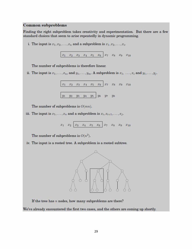
Embed Size (px)
Citation preview

1
09/15/2010
Recitation #2
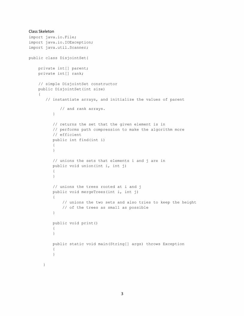
Lab Programming Assignment – Disjoint Sets Equivalence Relations
o A relation R is defined on a set S if for every pair of elements ( ) is either
true or false. If is true, then we say that a is related to b
o An equivalence relation is a relation R that satisfies three properties:
(Reflexive) , for all
(Symmetric) if and only if
(Transitive) and implies that
o Give an example Friends on Facebook (research that everybody is related within 5 -
7 degrees of people you know to anybody else on the planet)
Given an equivalence relation we want to decide if a and b are related we want to be
divided in equivalence classes every member of appears in exactly one equivalence class
sets are disjoint
Input is usually a collection of N sets, each with one element
Operations:
o Union(x, y) O(1)
Find roots for these two values
Merge these two trees into one
Try to minimize height of resulting tree attach smaller height to bigger height
subtree (union-by-height; there is also union-by-size)
Height increases only by 1 if trees of equal height are joined trivial
implementation
o Find(x) O(N)
Return root
o Path Compression is used to improve speed of Find operation
On the way to the root, every node’s parent is set to the root
Hard to recomputed heights when doing that
Heights are only estimated heights union-by-rank
Worst-Case of union-by-rank with path compression using M ( ) unions and finds is
( ) where is the number of times that logarithm of N needs to be applied until
result is , e.g.
o It’s a pain to prove check the book
ADT is usually optimized for fast “find” or fast “union” solution in book makes “union” easy
and “find” hard
Use arrays to store tree representation of set example
2
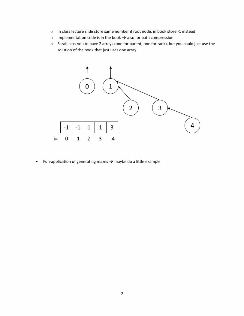
o In class lecture slide store same number if root node, in book store -1 instead
o Implementation code is in the book also for path compression
o Sarah asks you to have 2 arrays (one for parent, one for rank), but you could just use the
solution of the book that just uses one array
Fun-application of generating mazes maybe do a little example
0 1
2 3
4 -1 -1 1 3 1
i= 0 1 2 3 4
3
Class Skeleton import java.io.File;
import java.io.IOException;
import java.util.Scanner;
public class DisjointSet{
private int[] parent;
private int[] rank;
// simple DisjointSet constructor
public DisjointSet(int size)
{
// instantiate arrays, and initialize the values of parent
// and rank arrays.
}
// returns the set that the given element is in
// performs path compression to make the algorithm more
// efficient
public int find(int i)
{
}
// unions the sets that elements i and j are in
public void union(int i, int j)
{
}
// unions the trees rooted at i and j
public void mergeTrees(int i, int j)
{
// unions the two sets and also tries to keep the height
// of the trees as small as possible
}
public void print()
{
}
public static void main(String[] args) throws Exception
{
}
}
4
Recitation #3
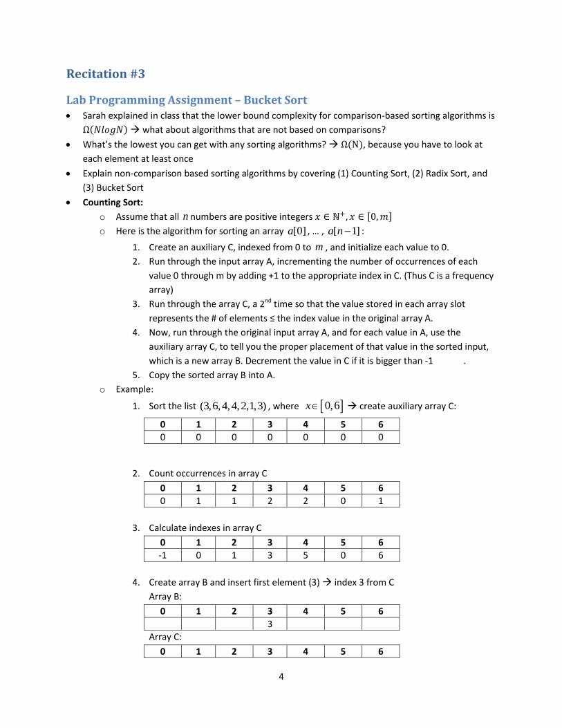
Lab Programming Assignment – Bucket Sort
Sarah explained in class that the lower bound complexity for comparison-based sorting algorithms is
( ) what about algorithms that are not based on comparisons?
What’s the lowest you can get with any sorting algorithms? ( ), because you have to look at
each element at least once
Explain non-comparison based sorting algorithms by covering (1) Counting Sort, (2) Radix Sort, and
(3) Bucket Sort
Counting Sort:
o Assume that all n numbers are positive integers [ ]
o Here is the algorithm for sorting an array [0]a , … , [ 1]a n :
1. Create an auxiliary C, indexed from 0 to m , and initialize each value to 0.
2. Run through the input array A, incrementing the number of occurrences of each
value 0 through m by adding +1 to the appropriate index in C. (Thus C is a frequency
array)
3. Run through the array C, a 2nd time so that the value stored in each array slot
represents the # of elements ≤ the index value in the original array A.
4. Now, run through the original input array A, and for each value in A, use the
auxiliary array C, to tell you the proper placement of that value in the sorted input,
which is a new array B. Decrement the value in C if it is bigger than -1 .
5. Copy the sorted array B into A.
o Example:
1. Sort the list (3,6,4,4,2,1,3) , where 0,6x create auxiliary array C:
0 1 2 3 4 5 6
0 0 0 0 0 0 0
2. Count occurrences in array C
0 1 2 3 4 5 6
0 1 1 2 2 0 1
3. Calculate indexes in array C
0 1 2 3 4 5 6
-1 0 1 3 5 0 6
4. Create array B and insert first element (3) index 3 from C
Array B:
0 1 2 3 4 5 6
3
Array C:
0 1 2 3 4 5 6
5
-1 0 1 2 5 0 6
4. Create array B and insert second element (6) index 6 from C
Array B:
0 1 2 3 4 5 6
3 6
Array C:
0 1 2 3 4 5 6
-1 0 1 2 5 0 5
…. (And so on with step 4)
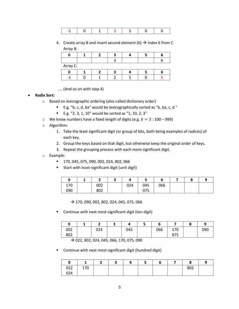
Radix Sort:
o Based on lexicographic ordering (also called dictionary order)
E.g. “b, c, d, ba" would be lexicographically sorted as "b, ba, c, d "
E.g. “2, 3, 1, 10” would be sorted as “1, 10, 2, 3”
o We know numbers have a fixed length of digits (e.g. : 100 – 999)
o Algorithm:
1. Take the least significant digit (or group of bits, both being examples of radices) of
each key.
2. Group the keys based on that digit, but otherwise keep the original order of keys.
3. Repeat the grouping process with each more significant digit.
o Example:
170, 045, 075, 090, 002, 024, 802, 066
Start with least-significant digit (unit digit)
0 1 2 3 4 5 6 7 8 9
170 090
002 802
024 045 075
066
170, 090, 002, 802, 024, 045, 075, 066
Continue with next most-significant digit (ten digit)
0 1 2 3 4 5 6 7 8 9
002 802
024 045 066 170 075
090
022, 802, 024, 045, 066, 170, 075, 090
Continue with next most-significant digit (hundred digit)
0 1 2 3 4 5 6 7 8 9
022 024
170 802
6
045 066 075 090
022, 024, 045, 066, 075, 090, 170, 802
o How would we do it for the most-significant digit Radix Sort?
o Running time ( ), where n is the number of keys, and k is the average key length
o Works also great for strings
Bucket Sort:
o Works best if elements are distributed uniformly between min and max We need
additional information about the input numbers
o floating-point numbers between ( ) and ( ): use buckets, each having the
range ( ( ) ( ) )
o Bucket indexing by ⌊ [ ] ( )
( ) ( )⌋ (for numbers between [ ) it would be ⌊ [ ]⌋).
just do an extra check if index is
o Algorithm:
1. Set up an array of initially empty "buckets."
2. Scatter: Go over the original array, putting each object in its bucket.
3. Sort each non-empty bucket. You can use something inefficient like insertion sort here:
( )
4. Gather: Visit the buckets in order and put all elements back into the original array.
o In its most basic form have one bucket for each value from [min, max]. Then go through
input array once and count elements by occurrence. Degenerated to Counting Sort
problem with memory, what to do about floating-point? ( ), where n is length of
input array, k length of counting array
Implementation:
o Verify that sorting is correct by using this isSorted() function in skeleton
o Implement linked list that automatically keeps order either with intelligently inserting
item or use Collections.sort() at the end on unsorted lists
o Implement Node (which is a bucket, that uses this linked list)
Why don’t we just use bucket sort for all sorting?
o Space requirements and overhead high constant can be worse than for reasonable
values of .
7
09/29/2010
Recitation #4 – Exam Review
Administrative Recitation # 2
o Grading Criteria changed correct handling of underscores
o WebCourses button “View Previous Comments”
Due date for bucket sort lab programs 11:59 p.m. tonight
Exam is tonight Panic !
Exam Review Go over proof for lower bound of comparison-based sorting see below
Series formulas
Where:
1 ... first term
... n-th termn
a
a
... number of elements
... common ratio
n
r
Finite geometric series of n elements (e.g. 1
2n
i
i
): 1(1 )
1
na rS
r
Finite arithmetic series of n elements (e.g. 1
n
i
i
): 1( )
2
nn a aS
Infinite geometric series (e.g. 1
1
2
i
i
): 1 , 11
aS r
r
Mixed arithmetic-geometric series try to get rid of geometric component by using the “S-Trick”
(Subtraction Trick)
S
xS
S xS
choose x to be the common ratio of geometric component
Big-Oh notation and definition
Definitions (here ( )f f n and ( )g g n ):
1. Big-Oh: ( )f O g iff 0( 0, 0)c n such that f cg for all 0n n
2. Big-Omega: ( )f g iff 0( 0, 0)c n such that f cg for all 0n n
3. Big-Theta: ( )f g iff ( )f O g and ( )f g
4. Little-Oh: ( )f o g iff ( )f O g and ( ) ( )f g g

8
o Simple Hierarchy: 2 2 3log log log 2Nc N N N N N N N
o How do you prove relationships analytically?
1. Look at the limit that the quotient of the two functions has:
0 ( )
lim 0 ( )
( )N
f o gf
c f gg
f g
o Always remember: ( ) ( )f O g g f
Sorting Algorithms Review
Counting Sort Demonstrated last time.
Radix Sort Demonstrated last time.
Bucket Sort Demonstrated last time.
Shell Sort
Merge Sort Should know by now
Quick Sort Should know by now
Shell Sort
Best case ( )O N , Worst case 2( log )O N N
The basic idea:
Instead of sorting all the elements at once, sort a small set of them
Such as every 5th element (you can use insertion sort)
Then sort every 3rd element, etc.
Finally sort all the elements using insertion sort.
Rationale:
A small insertion sort is quite efficient.
A larger insertion sort can be efficient, if the elements are already “close” to sorted order.
By doing the smaller insertion sorts, the elements do get closer to in order before the larger
insertions are done.
Example (Elements with the same color are in the same sorting set):
Select every 5th element
Sort sets of elements and select every 3rd element
Sort sets of elements and select all elements
Final Insertion Sort Result
9
Works best when increment sequence is geometric series in which every term is approximately 2.2
times smaller than the previous one
AVL Trees
Binary Tree with balance condition
At any node, the difference of height between the left and right subtree is at most 1
Insertion Average and Worst Case (log )O N
- Insert in tree and trace up towards root and see if there is an imbalance at any node
- For cases 2 and 3, starting from , list nodes 1 2 3, ,k k k in-order Always make 2k the new
root
- 4 possibilities of what can happen:
1. Insertion into the left subtree of the left child of
2. Insertion into the right subtree of the left child of
3. Insertion into the left subtree of the right child of
4. Insertion into the right subtree of the right child of
Deletion Average and Worst Case (log )O N
10
1. If the node is a leaf, remove it. Retrace back up the tree starting with the parent of deleted
node to the root, adjusting the balance factor as needed single or double rotation might
be necessary.
2. If it’s not a leaf, replace with the largest in its left subtree (inorder predecessor) and remove
that node. (or replace with the smallest in its right subtree (inorder successor)).
3. After deletion, retrace the path back up the tree, starting with the parent of the
replacement, to the root, adjusting the balance factor as needed.
Search Average and Worst Case (log )O N
2-4 Trees
o Specific type of multitree.
o Every node must have in between 2 and 4 children. (Thus each internal node must store in
between 1 and 3 keys)
o All external nodes (the null children of leaf nodes) and leaf nodes have the same depth.
o Left subtree of a key always contains values that are than key, right subtree always has
values that are
o Insertion: (log )O N
1. Wiggle your way through to leaf node
2. If leaf node becomes full, send 3rd value to parents and split the other 3 values
3. If parent is not able to accept new value, repeat the procedure and make new root
o Deletion: (log )O N
11
See attached printout
o Search: (log )O N
Binary Heaps
Similar to binary search tree, but ALL values in the subtree rooted at a node are (min heap)
Used in priority queue and for Heap Sort
Store in array, children of node i are nodes 2i and (2 1)i , parent of node i is / 2i
Insertion (log )O n
o Insert in next open spot in the heap might be wrong spot
o Percolate up is necessary
o If the parent of the new node is greater than the inserted value, swap them.
(a single percolate up step)
o Continue this process until the inserted node’s parent stores a number lower than it.
o Since the height of the tree is (log )O n , this is an (log )O n operation.
Deletion (deleteMin) (log )O n
o Return value stored in the root
o Place the “last” node in the vacated root; Probably not the correct location.
o Percolate Down
1. Compare the element to its children.
2. If one of the children is less than the node, swap the lowest.
(This is a single percolate down step)
3. CONTINUE until this “last” node has children with larger values than it.
Heapify (MakeHeap) ( )O n after careful anlysis
o Construct heap out of unsorted elements
o Place all the unsorted elements in a complete binary tree.
o Going through the nodes in backwards order, and skipping the leaf nodes, run Percolate
Down on each of these nodes.
o Notice that each subtree below any node that has already run Percolate Down is already a
heap. So after we run Percolate Down on the root, the whole tree is a heap.
12
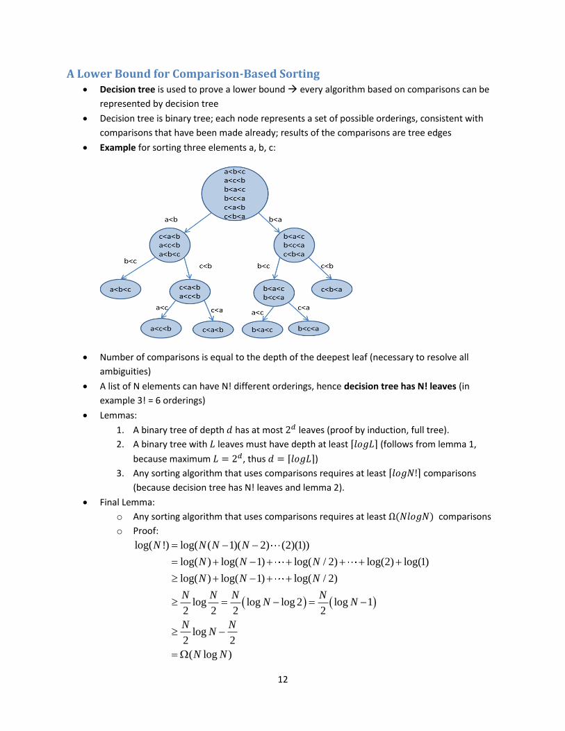
A Lower Bound for Comparison-Based Sorting Decision tree is used to prove a lower bound every algorithm based on comparisons can be
represented by decision tree
Decision tree is binary tree; each node represents a set of possible orderings, consistent with
comparisons that have been made already; results of the comparisons are tree edges
Example for sorting three elements a, b, c:
Number of comparisons is equal to the depth of the deepest leaf (necessary to resolve all
ambiguities)
A list of N elements can have N! different orderings, hence decision tree has N! leaves (in
example 3! = 6 orderings)
Lemmas:
1. A binary tree of depth has at most leaves (proof by induction, full tree).
2. A binary tree with leaves must have depth at least ⌈ ⌉ (follows from lemma 1,
because maximum , thus ⌈ ⌉)
3. Any sorting algorithm that uses comparisons requires at least ⌈ ⌉ comparisons
(because decision tree has N! leaves and lemma 2).
Final Lemma:
o Any sorting algorithm that uses comparisons requires at least ( ) comparisons
o Proof:
log( !) log( ( 1)( 2) (2)(1))
log( ) log( 1) log( / 2) log(2) log(1)
log( ) log( 1) log( / 2)
log log log 2 log 12 2 2 2
log2 2
( log )
N N N N
N N N
N N N
N N N NN N
N NN
N N
13
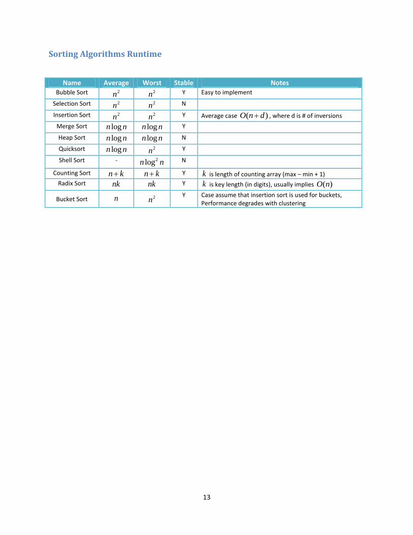
Sorting Algorithms Runtime
Name Average Worst Stable Notes Bubble Sort 2n
2n Y Easy to implement
Selection Sort 2n 2n N
Insertion Sort 2n 2n Y Average case ( )O n d , where d is # of inversions
Merge Sort logn n logn n Y
Heap Sort logn n logn n N
Quicksort logn n 2n Y
Shell Sort - 2logn n N
Counting Sort n k n k Y k is length of counting array (max – min + 1)
Radix Sort nk nk Y k is key length (in digits), usually implies ( )O n
Bucket Sort n 2n Y Case assume that insertion sort is used for buckets,
Performance degrades with clustering
14
10/13/2010
Recitation #5
Assignment #3 Due on 10/20/2010, 11:59 p.m. (only have one week’s time)
You basically have an undirected, weighted graph; survivors are nodes and edges are given as
weighted paths between survivors in the input file
It is guaranteed that the graph is connected, i.e. all nodes/survivors are reachable
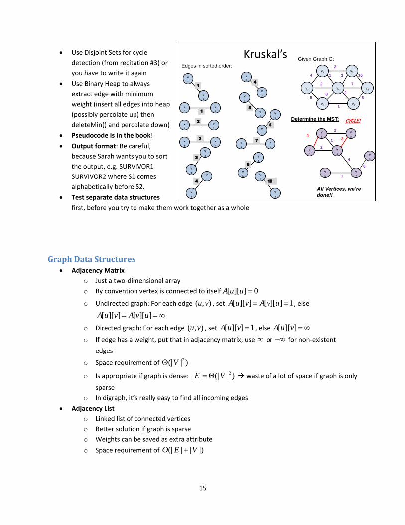
Implement Kruskal’s Algorithm for calculating a Minimum Spanning Tree
o MST of weighted, undirected graph is tree formed by connecting all of the vertices with
minimal overall cost
o minimum cost Minimum; covers every vertex Spanning; Acyclic Tree
o There could be multiple MSTs (all with the same minimum weight)
o From Lecture Slides:
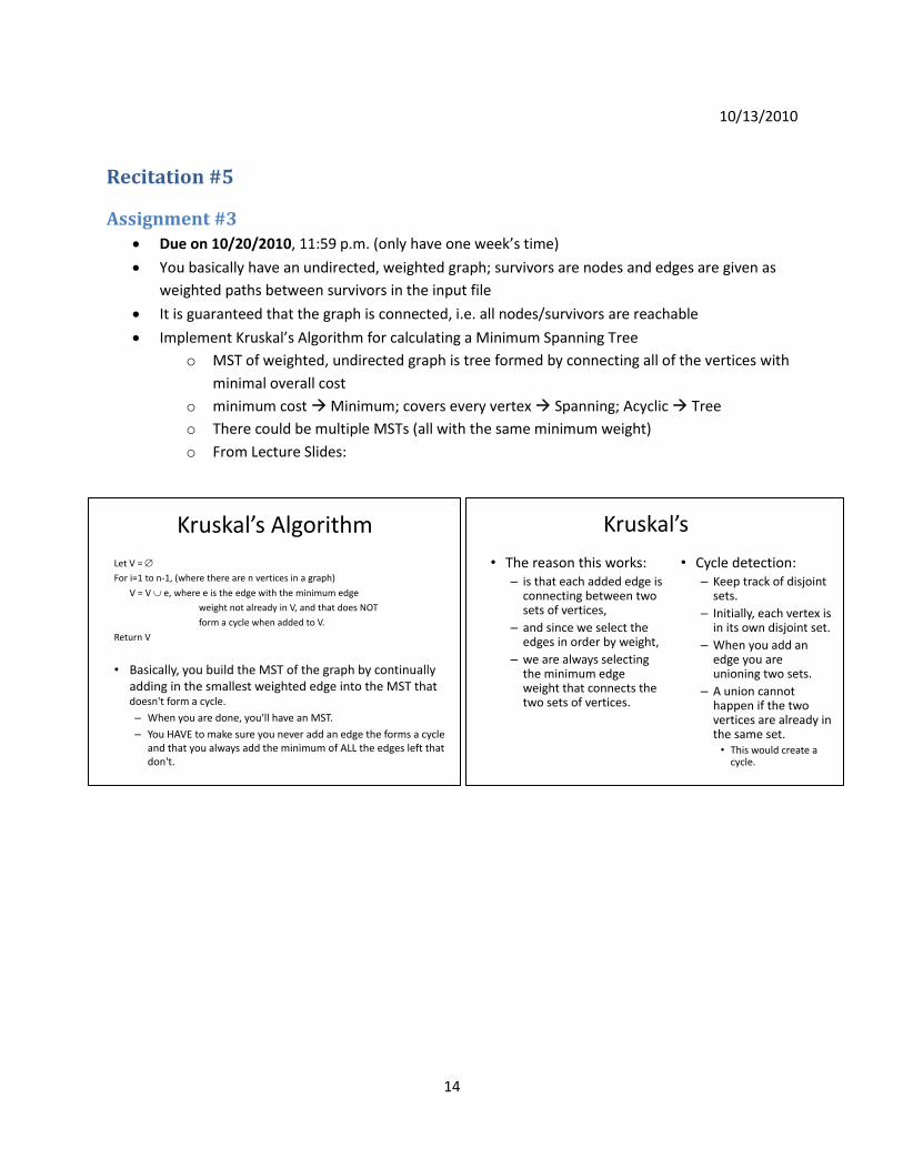
Kruskal’s Algorithm
Let V =
For i=1 to n-1, (where there are n vertices in a graph)
V = V e, where e is the edge with the minimum edge
weight not already in V, and that does NOT
form a cycle when added to V.
Return V
• Basically, you build the MST of the graph by continually adding in the smallest weighted edge into the MST that doesn't form a cycle.
– When you are done, you'll have an MST.
– You HAVE to make sure you never add an edge the forms a cycle and that you always add the minimum of ALL the edges left that don't.
Kruskal’s
• The reason this works: – is that each added edge is
connecting between two sets of vertices,
– and since we select the edges in order by weight,
– we are always selecting the minimum edge weight that connects the two sets of vertices.
• Cycle detection:– Keep track of disjoint
sets.
– Initially, each vertex is in its own disjoint set.
– When you add an edge you are unioning two sets.
– A union cannot happen if the two vertices are already in the same set.• This would create a
cycle.
15
Use Disjoint Sets for cycle
detection (from recitation #3) or
you have to write it again
Use Binary Heap to always
extract edge with minimum
weight (insert all edges into heap
(possibly percolate up) then
deleteMin() and percolate down)
Pseudocode is in the book!
Output format: Be careful,
because Sarah wants you to sort
the output, e.g. SURVIVOR1
SURVIVOR2 where S1 comes
alphabetically before S2.
Test separate data structures
first, before you try to make them work together as a whole
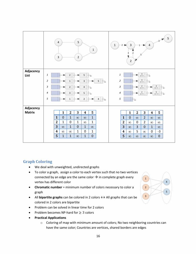
Graph Data Structures Adjacency Matrix
o Just a two-dimensional array
o By convention vertex is connected to itself [ ][ ] 0A u u
o Undirected graph: For each edge ( , )u v , set [ ][ ] [ ][ ] 1A u v A v u , else
[ ][ ] [ ][ ]A u v A v u
o Directed graph: For each edge ( , )u v , set [ ][ ] 1A u v , else [ ][ ]A u v
o If edge has a weight, put that in adjacency matrix; use or for non-existent
edges
o Space requirement of 2(| | )V
o Is appropriate if graph is dense: 2| | (| | )E V waste of a lot of space if graph is only
sparse
o In digraph, it’s really easy to find all incoming edges
Adjacency List
o Linked list of connected vertices
o Better solution if graph is sparse
o Weights can be saved as extra attribute
o Space requirement of (| | | |)O E V
Kruskal’sv1
v7v6
v4v3 v5
v2
1
4
2
4
2
8
31 10
7
65
v1
v4
1
v1
v4
1
v7
v6 1
v7
v6 1
v1
v2
2
v4
v3
2
v4
v2
3
v7
v4
4
v6
v3
5
v7
v5
6
v1
v3
4
v4
v5
7
v6
v4
8
v5
v2
10
v2
2
v3
2
3
CYCLE!
4
4
v5
6
All Vertices, we’re
done!!
Determine the MST:
Edges in sorted order:
Given Graph G:
16
1
4 5
3 2
1 4
5
3
2
2
3 2
1
5
-3
Adjacency List 1
2
3
4
5
2 55
11 33 55
22 44
33 55
11 22 44
1
2
3
4
5
3w = 2
3w = 2
2w = 3
4w = 1
2w = 5
5w = -3
Adjacency Matrix 1 2 3 4 5
1 0 1 1
2 1 0 1 1
3 1 0 1 4 1 0 1
5 1 1 1 0
1 2 3 4 5
1 0 2 2 0 2 3 3 0 1 4 5 0 -3
5 0
Graph Coloring We deal with unweighted, undirected graphs
To color a graph, assign a color to each vertex such that no two vertices
connected by an edge are the same color in complete graph every
vertex has different color
Chromatic number = minimum number of colors necessary to color a
graph
All bipartite graphs can be colored in 2 colors ↔ All graphs that can be
colored in 2 colors are bipartite
Problem can be solved in linear time for 2 colors
Problem becomes NP-hard for colors
Practical Applications
o Coloring of map with minimum amount of colors; No two neighboring countries can
have the same color; Countries are vertices, shared borders are edges
14
5
3
2

17
o Aquarium Mix; For a number of fish species decide how many tanks are needed to
house all of them, so they don’t eat each other; Fish Species are vertices; Predator-Prey
relationships are edges in graph; Chromatic Number equals minimum amount of tanks
that you need so fish don’t eat each other
Graph Search Methods Depth-First Search
o Search down a path from a particular source vertex as far as possible
o When you can go no farther, backtrack to last vertex from which a different path could
have been taken
o Continue that until all vertices covered
o Mark edges and vertices that have already been visited
Breadth-First Search
o Opposite of Depth-First Search
o Search all paths at a uniform depth from the source before moving onto deeper paths.
o Mark edges and vertices that have already been visited
Lab Programming Assignment – 2-Coloring of a Graph Due date: 10/20/2010, 11:59 p.m.
Use one of the data structures (adjacency matrix, adjacency list) to save the graph
Run Breadth-First Search
o Implementation suggestion in lecture notes and in the book
Depth First Search
• Start with 1• 2,4,3
– Stop at 3
• Backtrack to 4, can we search?• 7,6
– Stop at 2
• Backtrack to 6, can we search?• 10,13
– Stop at 13
• Backtrack to 10,6,7• 9, 11, 8, 5
– Stop at 5
• Backtrack to 8,11• 15,14,12
– STOP – All nodes are marked!!
1 2 5
106
11 15
3 4 7 129
13
14
8
Output
List:
1 2 4 3 7 6 10 13 9 11 8 5 15 14 12
1 2
3
5
6
11
4
10
15
7 9
8
12
13
14
Breadth First Search
• L0: 1• L1: 2, 3• L2: 4,5,6,11• L3: 7,8,10,9,15• L4: 13,12,14
1 2 5
106
11 15
3 4 7 129
13
14
1 2
3
5
6
11
4
8
10
15
7 9
8
12
13
14
Final output: 1, 2, 3, 4, 5, 6, 11, 7, 8, 10, 9, 15, 13, 12, 14
18
10/20/2010
Recitation #6
Most common sources of errors for students
1. Make up your own test cases. Many students just rely on the test cases on the assignment sheet or the additional test cases you give them, rather than making up their own and testing the code extensively.
2. Modularity. Students should learn to develop and test the code in stages/modules. One thing I noticed a lot in office hours is that students think of their code as this monolithic black box that should take your input file and print the desired output. If that doesn't work, they tinker in all kinds of different places without actually knowing what components of the code are actually working and which are the culprit for the faulty output. Assignment #3 was a perfect example for that. Students should first develop a working heap and test it before they go on. Then implement the Disjoint Sets and run through the same tests. Only once this is all done, put everything together and connect the dots. If there are any errors in this last stage you can exclude the Disjoint Sets and the binary heap from your search, because you already verified these modules.
3. Debugging. This relates to (2), but I think any programmer should know how to use a graphical debugger. No matter what IDE you use to develop your code, it will include a graphical debugger. You can set breakpoints, watch variable values change, and step through the code line-by-line if necessary. Many students still rely on printouts in their code, which makes finding bugs a lot harder. I will try to encourage students in my labs tomorrow to familiarize themselves with the Eclipse debugger for their next assignment
Using Eclipse Debugger Please NEVER use printouts for debugging your code
A Graphical debugger is the way to go every IDE has a good debugger built-in
Great way to see variable values and trace through code
Click on the little “bug” icon instead of the run icon to start debugging mode it will ask you to
change to the debugging perspective
Right-click on the vertical bar at the left of the source file and select “Toggle Breakpoint”
o A breakpoint will stop code execution at that line
o You can set conditions on when this breakpoint should trigger
o Once the program stops you can see the value of all variables
o You can step through the code line-by-line and make sure that everything works the way
you want it
Just search for “Eclipse Debugger” and you should find a wealth of websites and tutorials
19
Greedy Bottom-up approach
Greedy takes the step that seems the best at the time of execution; very short-sighted and
looking for immediate gain, i.e. “greedy”
Greedy algorithms try to make locally optimal decisions hoping that this will contribute to a
globally optimal solution
E.g. Dijkstra’s, Kruskal’s, Prim’s
Divide-And-Conquer Top-Down approach
Traditionally, algorithms with at least 2 recursive calls are divide-and-conquer, while algorithms
with one (e.g. find() in Disjoint Sets) are not
Works as follows:
o If the problem is small enough, solve it (base case). Else:
o Divide: Divide big problem into smaller disjoint subproblems.
o Conquer: Solve subproblems recursively.
o Combine: The solution to the original problem is then formed from the solutions of the
subproblems
Because of recursion, timing analysis often involves recurrences, e.g. ( ) ( / 2) ( )T n T n O n
User Master Theorem for those
E.g. Quicksort, Mergesort, Integer Multiplication, Strassen’s
Recurrence Relations If an algorithm contains a recursive call to itself its running time can often be described by a
recurrence relation, e.g.
(1) if 1( )
2 ( / 2) ( ) if 1
nT n
T n n n
this is MergeSort’s runtime
Different ways to solve that:
1. Telescoping Method:
o Write the recurrence equation repeatedly “following” the recurrence
20
o Adding up all equations usually leads to cancellation of a lot of terms
o E.g. ( ) ( 1)T N T N cN
Write out equation repeatedly:
( 1) ( 2) ( 1)
( 2) ( 3) ( 2)
(2) (1) (2)
T N T N c N
T N T N c N
T T c
Adding up all the equations yields:
( ) ( 1) (2) ( 1) (1) 2T N T N T T N T cN c
Subtracting all duplicate terms gives the solution:
2
2
( ) (1)
( )
N
i
T N T c i
O N
o E.g. ( ) 2 ( / 2)T N T N N
Same steps as above, but witch little twist that I divide by N first:
( ) ( / 2)1
/ 2
T N T N
N N
Then do the telescoping:
( / 2) ( / 4)1
/ 2 / 4
(2) (1)1
2 1
T N T N
N N
T T
Adding the equations and subtracting duplicate terms:
( ) (1)log
1
( ) log ( log )
T N TN
N
T N N N N O N N
2. Substitution Method:
o Substitute the recurrence repeatedly on the right side
o Look for a pattern and solve
o E.g. ( ) ( 1)T N T N cN
Substitute repeatedly:
21
2
2
( ) ( 2) ( 1)
( 3) ( 2) ( 1)
(1) (2) ( 1)
(1) ( )N
i
T N T N c N
T N c N c N
T c c N
T c i O N
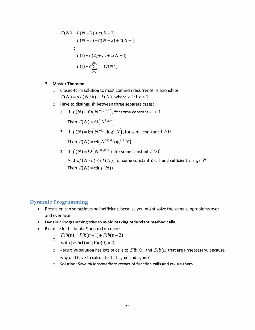
3. Master Theorem:
o Closed-form solution to most common recurrence relationships
( ) ( / ) ( )T N aT N b f N , where 1, 1a b
o Have to distinguish between three separate cases:
1. If log( ) b a
f N O N
, for some constant 0
Then log( ) b a
T N N
2. If log( ) logb a kf N N N , for some constant 0k
Then log 1( ) logb a kT N N N
3. If log( ) b a
f N N
, for some constant 0
And ( / ) ( )af N b cf N , for some constant 1c and sufficiently large N
Then ( ) ( ( ))T N f N
Dynamic Programming Recursion can sometimes be inefficient, because you might solve the same subproblems over
and over again
Dynamic Programming tries to avoid making redundant method calls
Example in the book: Fibonacci numbers:
o ( ) ( 1) ( 2)
with [ (1) 1; (0) 0]
Fib n Fib n Fib n
Fib Fib
o Recursive solution has lots of calls to (0)Fib and (1)Fib that are unnecessary, because
why do I have to calculate that again and again?
o Solution: Save all intermediate results of function calls and re-use them
22
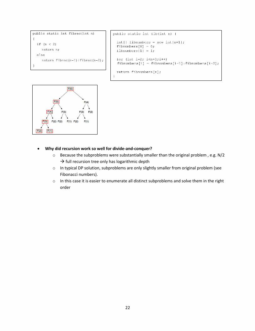
Why did recursion work so well for divide-and-conquer?
o Because the subproblems were substantially smaller than the original problem , e.g. N/2
full recursion tree only has logarithmic depth
o In typical DP solution, subproblems are only slightly smaller from original problem (see
Fibonacci numbers).
o In this case it is easier to enumerate all distinct subproblems and solve them in the right
order

23
Subset Sum Divide-And-Conquer solution This method to solve a variant of the subset sum problem was discussed by Sarah in class
Lab Programming Assignment Solve the subset sum problem with Dynamic Programming
From Sarah’s E-Mail: “If you could review this and also describe how it makes redundant
recursive calls, so a dynamic programming solution would be faster that would be great. Then if
they need a hint on how to implement the Dynamic Programming version, suggest a boolean
array of size target+1 and describe what those boolean values correspond to. They will probably
also need an example to show this. I suggest a target of 8 and values array [4, 3, 4, 2] since
that's what we used in class. “
From Wikipedia:
24
10/27/2010
Recitation – Exam Review for Exam 2
Exam Review Make sure you understand how most of the presented algorithms work in principle
Mostly driven by students’ questions
If they are not forthcoming, definitely cover the following topics: Master Theorem, Topological Sort
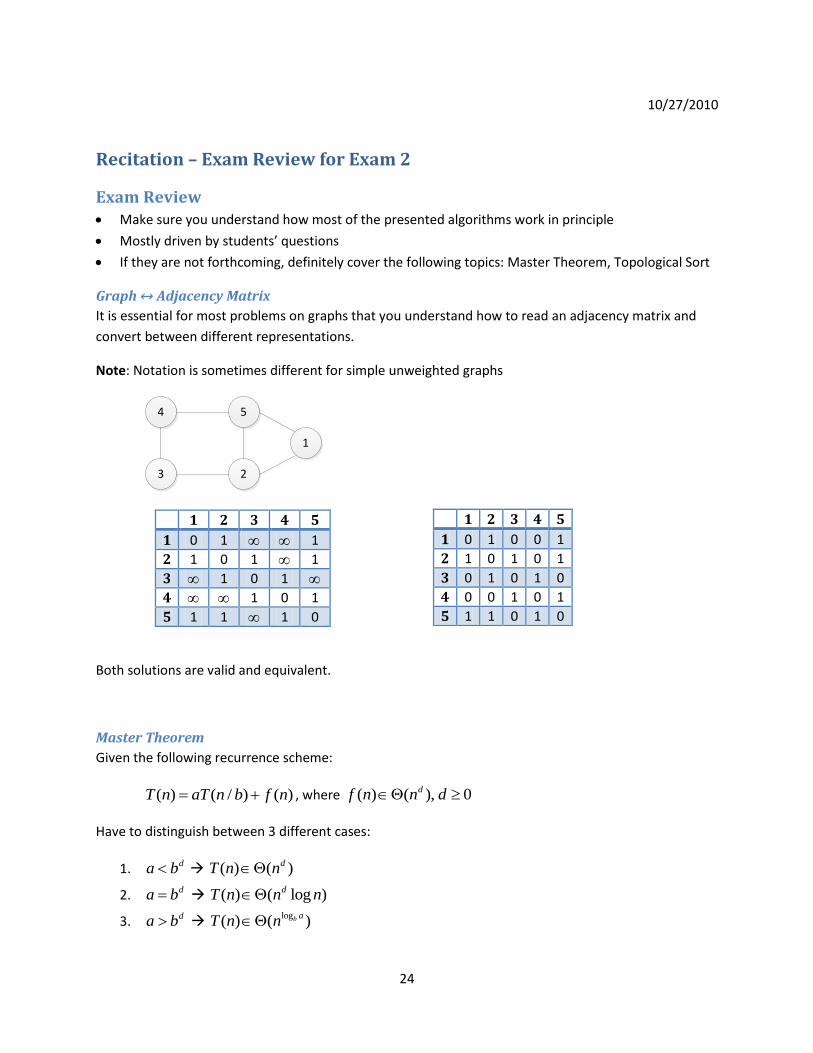
Graph ↔ Adjacency Matrix
It is essential for most problems on graphs that you understand how to read an adjacency matrix and
convert between different representations.
Note: Notation is sometimes different for simple unweighted graphs
1
4 5
3 2
1 2 3 4 5
1 0 1 1
2 1 0 1 1
3 1 0 1 4 1 0 1
5 1 1 1 0
Both solutions are valid and equivalent.
Master Theorem
Given the following recurrence scheme:
( ) ( / ) ( )T n aT n b f n , where ( ) ( ), 0df n n d
Have to distinguish between 3 different cases:
1. da b ( ) ( )dT n n
2. da b ( ) ( log )dT n n n
3. da b log( ) ( )b a
T n n
1 2 3 4 5
1 0 1 0 0 1
2 1 0 1 0 1
3 0 1 0 1 0
4 0 0 1 0 1
5 1 1 0 1 0
25
Be careful, because you cannot use it for non-divisive recurrences e.g. ( ) ( 1) ( )T n T n O n Use
telescoping or substitution instead. The only thing you will have to do in the exam is being able to apply
the Master Theorem.
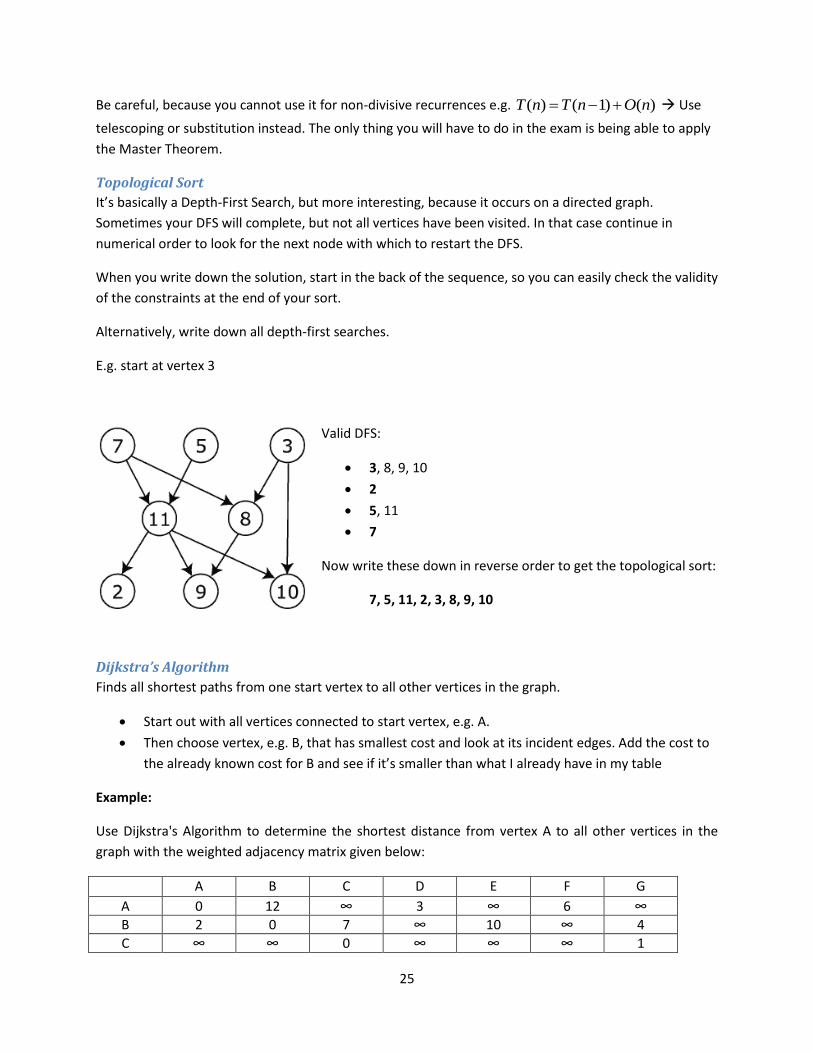
Topological Sort
It’s basically a Depth-First Search, but more interesting, because it occurs on a directed graph.
Sometimes your DFS will complete, but not all vertices have been visited. In that case continue in
numerical order to look for the next node with which to restart the DFS.
When you write down the solution, start in the back of the sequence, so you can easily check the validity
of the constraints at the end of your sort.
Alternatively, write down all depth-first searches.
E.g. start at vertex 3
Valid DFS:
3, 8, 9, 10
2
5, 11
7
Now write these down in reverse order to get the topological sort:
7, 5, 11, 2, 3, 8, 9, 10
Dijkstra’s Algorithm
Finds all shortest paths from one start vertex to all other vertices in the graph.
Start out with all vertices connected to start vertex, e.g. A.
Then choose vertex, e.g. B, that has smallest cost and look at its incident edges. Add the cost to
the already known cost for B and see if it’s smaller than what I already have in my table
Example:
Use Dijkstra's Algorithm to determine the shortest distance from vertex A to all other vertices in the
graph with the weighted adjacency matrix given below:
A B C D E F G
A 0 12 ∞ 3 ∞ 6 ∞ B 2 0 7 ∞ 10 ∞ 4 C ∞ ∞ 0 ∞ ∞ ∞ 1
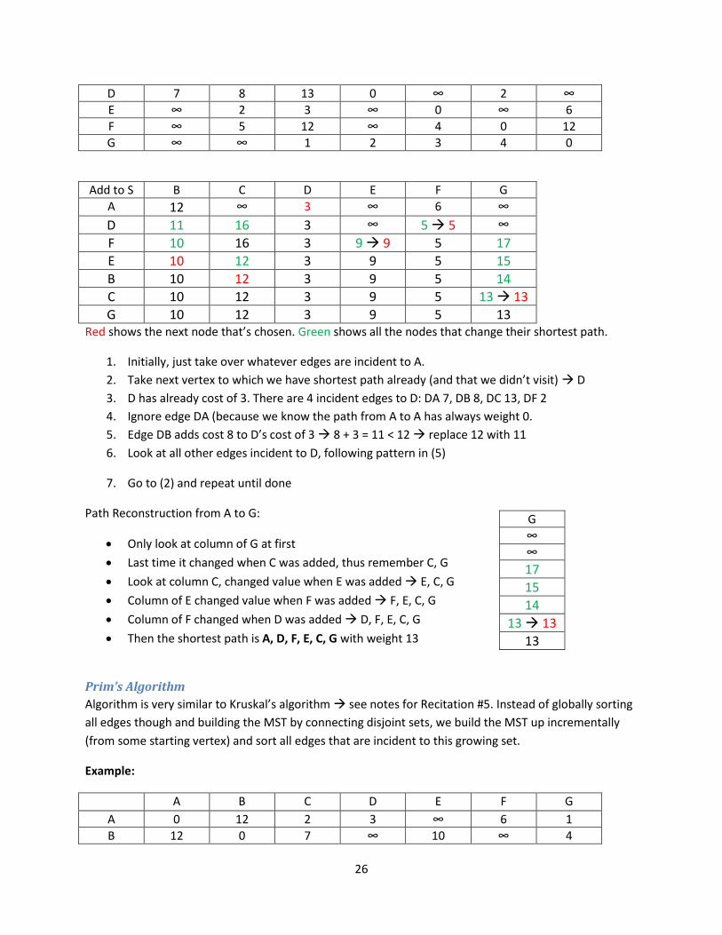
26
D 7 8 13 0 ∞ 2 ∞ E ∞ 2 3 ∞ 0 ∞ 6 F ∞ 5 12 ∞ 4 0 12 G ∞ ∞ 1 2 3 4 0
Add to S B C D E F G A 12 ∞ 3 ∞ 6 ∞
D 11 16 3 ∞ 5 5 ∞
F 10 16 3 9 9 5 17
E 10 12 3 9 5 15
B 10 12 3 9 5 14
C 10 12 3 9 5 13 13
G 10 12 3 9 5 13 Red shows the next node that’s chosen. Green shows all the nodes that change their shortest path.
1. Initially, just take over whatever edges are incident to A.
2. Take next vertex to which we have shortest path already (and that we didn’t visit) D
3. D has already cost of 3. There are 4 incident edges to D: DA 7, DB 8, DC 13, DF 2
4. Ignore edge DA (because we know the path from A to A has always weight 0.
5. Edge DB adds cost 8 to D’s cost of 3 8 + 3 = 11 < 12 replace 12 with 11
6. Look at all other edges incident to D, following pattern in (5)
7. Go to (2) and repeat until done
Path Reconstruction from A to G:
Only look at column of G at first
Last time it changed when C was added, thus remember C, G
Look at column C, changed value when E was added E, C, G
Column of E changed value when F was added F, E, C, G
Column of F changed when D was added D, F, E, C, G
Then the shortest path is A, D, F, E, C, G with weight 13
Prim’s Algorithm
Algorithm is very similar to Kruskal’s algorithm see notes for Recitation #5. Instead of globally sorting
all edges though and building the MST by connecting disjoint sets, we build the MST up incrementally
(from some starting vertex) and sort all edges that are incident to this growing set.
Example:
A B C D E F G
A 0 12 2 3 ∞ 6 1 B 12 0 7 ∞ 10 ∞ 4
G ∞ ∞ 17
15
14
13 13
13
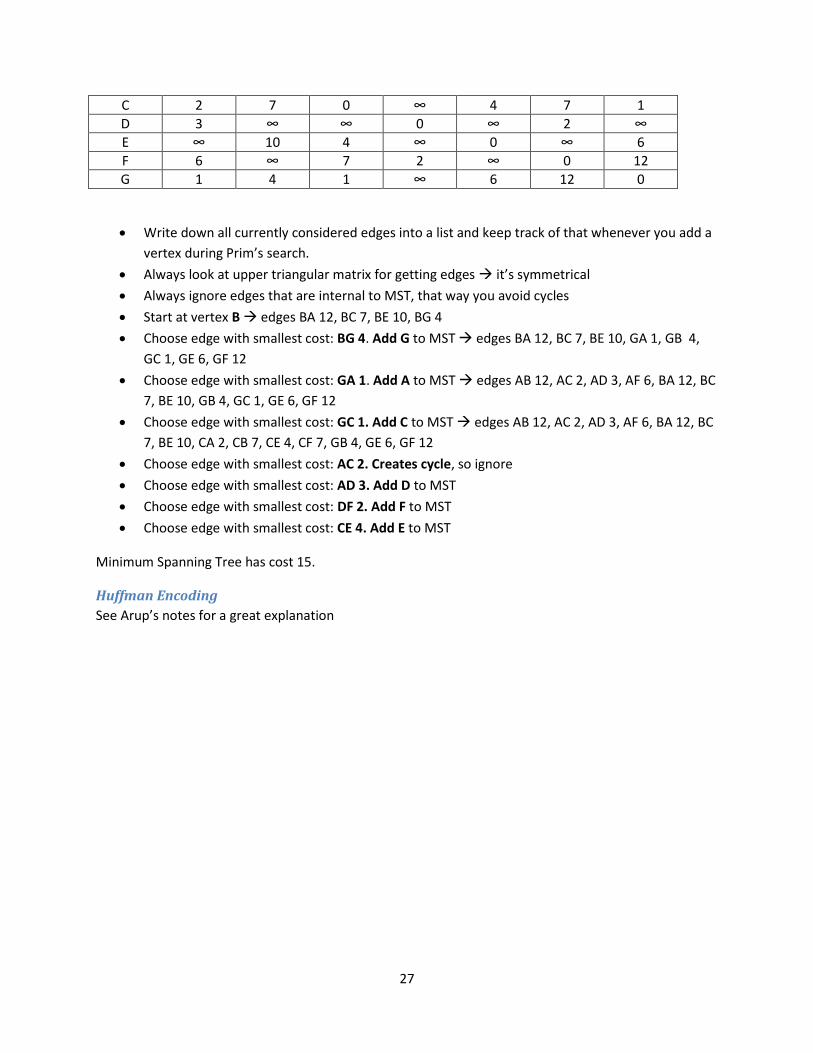
27
C 2 7 0 ∞ 4 7 1 D 3 ∞ ∞ 0 ∞ 2 ∞ E ∞ 10 4 ∞ 0 ∞ 6 F 6 ∞ 7 2 ∞ 0 12 G 1 4 1 ∞ 6 12 0
Write down all currently considered edges into a list and keep track of that whenever you add a
vertex during Prim’s search.
Always look at upper triangular matrix for getting edges it’s symmetrical
Always ignore edges that are internal to MST, that way you avoid cycles
Start at vertex B edges BA 12, BC 7, BE 10, BG 4
Choose edge with smallest cost: BG 4. Add G to MST edges BA 12, BC 7, BE 10, GA 1, GB 4,
GC 1, GE 6, GF 12
Choose edge with smallest cost: GA 1. Add A to MST edges AB 12, AC 2, AD 3, AF 6, BA 12, BC
7, BE 10, GB 4, GC 1, GE 6, GF 12
Choose edge with smallest cost: GC 1. Add C to MST edges AB 12, AC 2, AD 3, AF 6, BA 12, BC
7, BE 10, CA 2, CB 7, CE 4, CF 7, GB 4, GE 6, GF 12
Choose edge with smallest cost: AC 2. Creates cycle, so ignore
Choose edge with smallest cost: AD 3. Add D to MST
Choose edge with smallest cost: DF 2. Add F to MST
Choose edge with smallest cost: CE 4. Add E to MST
Minimum Spanning Tree has cost 15.
Huffman Encoding
See Arup’s notes for a great explanation
28
11/03/2010
Recitation #7
Dynamic Programming Review:
o Recursion can sometimes be inefficient, because you might solve the same subproblems
over and over again
o Dynamic Programming tries to avoid making redundant method calls
A few more notes on the subject:
o Optimal substructure:
optimal solution can be constructed efficiently from optimal solutions to its
subproblems
typically use Greedy algorithms for that, but if the problem also exhibits
overlapping subproblems, we use DP
Nice examples (from Wikipedia):
Shortest path between two cities is likely to exhibit optimal
substructure. That is, if the shortest route from Seattle to Los Angeles
passes through Portland and then Sacramento, then the shortest route
from Portland to Los Angeles must pass through Sacramento too.
Problem of finding the cheapest airline ticket from Buenos Aires to
Moscow. Even if that ticket involves stops in Miami and then London, we
can't conclude that the cheapest ticket from Miami to Moscow stops in
London, because the price at which an airline sells a multi-flight trip is
usually not the sum of the prices at which it would sell the individual
flights in the trip.
o Overlapping subproblems:
Problem can be broken down into subproblems which are reused several times
Think of the Fibonacci sequence and how terms were used over and over again
29

30
Longest Common Subsequence DP Solution Solved by Sarah in class
See attached sheet
Example of recursive solution:
LCS(“BEER”, “BEAR”)
LCS(“BEE”, “BEA”)1 +
LCS(“BE”, “BEA”) LCS(“BEE”, “BE”)MAX( )
LCS(“BE”, “B”)1 +LCS(“B”, “BEA”) LCS(“BE”, “BE”)MAX( )
LCS(“B”, “B”)1 +
1
2
1
1
2
2
2
3
Example of DP solution:
= LCS(“BE”, “BE”) = 1 + LCS(“B”, ”B”) [1 + value from up and left cell in table]
= LCS(“BEER”, “BEA”) = MAX( LCS(“BEE”, “BEA”), LCS(“BEER, “BE”) )
[max of values from top and left cells in table]
B E A R
B 1 1 1 1
E 1 2 2 2
E 1 2 2 2
R 1 2 2 3
o Reconstructing the LCS sequence in string form
Start on bottom right cell construct string backwards
If characters match, take it and go diagonally to the top left
If characters don’t match, choose the maximum of the cell to the left or the cell
to the top and continue there
LCS(“BEER”, “BEAR”) = “BER”
2
2
B E A R
B 1 1 1 1
E 1 2 2 2
E 1 2 2 2
R 1 2 2 3
31
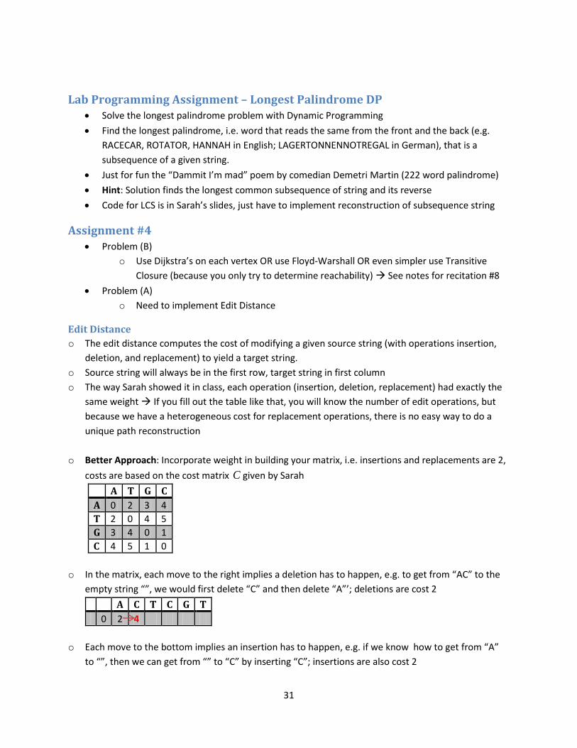
Lab Programming Assignment – Longest Palindrome DP Solve the longest palindrome problem with Dynamic Programming
Find the longest palindrome, i.e. word that reads the same from the front and the back (e.g.
RACECAR, ROTATOR, HANNAH in English; LAGERTONNENNOTREGAL in German), that is a
subsequence of a given string.
Just for fun the “Dammit I’m mad” poem by comedian Demetri Martin (222 word palindrome)
Hint: Solution finds the longest common subsequence of string and its reverse
Code for LCS is in Sarah’s slides, just have to implement reconstruction of subsequence string
Assignment #4 Problem (B)
o Use Dijkstra’s on each vertex OR use Floyd-Warshall OR even simpler use Transitive
Closure (because you only try to determine reachability) See notes for recitation #8
Problem (A)
o Need to implement Edit Distance
Edit Distance
o The edit distance computes the cost of modifying a given source string (with operations insertion,
deletion, and replacement) to yield a target string.
o Source string will always be in the first row, target string in first column
o The way Sarah showed it in class, each operation (insertion, deletion, replacement) had exactly the
same weight If you fill out the table like that, you will know the number of edit operations, but
because we have a heterogeneous cost for replacement operations, there is no easy way to do a
unique path reconstruction
o Better Approach: Incorporate weight in building your matrix, i.e. insertions and replacements are 2,
costs are based on the cost matrix C given by Sarah
A T G C
A 0 2 3 4
T 2 0 4 5
G 3 4 0 1
C 4 5 1 0
o In the matrix, each move to the right implies a deletion has to happen, e.g. to get from “AC” to the
empty string “”, we would first delete “C” and then delete “A”’; deletions are cost 2
A C T C G T
0 2 4
o Each move to the bottom implies an insertion has to happen, e.g. if we know how to get from “A”
to “”, then we can get from “” to “C” by inserting “C”; insertions are also cost 2
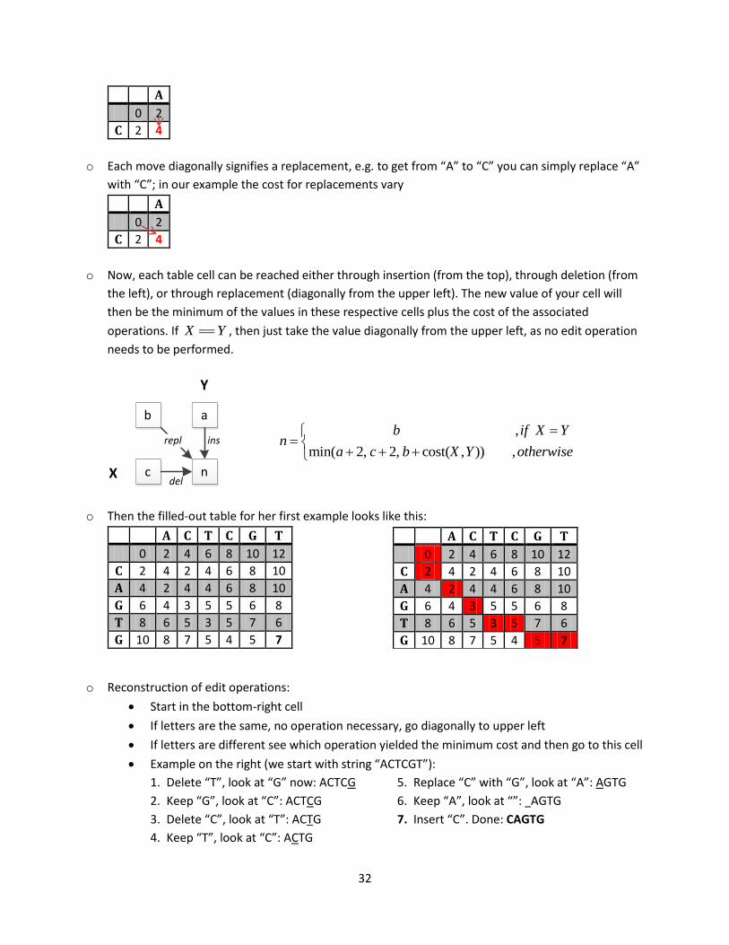
32
A
0 2
C 2 4
o Each move diagonally signifies a replacement, e.g. to get from “A” to “C” you can simply replace “A”
with “C”; in our example the cost for replacements vary
A
0 2
C 2 4
o Now, each table cell can be reached either through insertion (from the top), through deletion (from
the left), or through replacement (diagonally from the upper left). The new value of your cell will
then be the minimum of the values in these respective cells plus the cost of the associated
operations. If X Y , then just take the value diagonally from the upper left, as no edit operation
needs to be performed.
,
min( 2, 2, cost( , )) ,
b if X Yn
a c b X Y otherwise
o Then the filled-out table for her first example looks like this:
A C T C G T
0 2 4 6 8 10 12
C 2 4 2 4 6 8 10
A 4 2 4 4 6 8 10
G 6 4 3 5 5 6 8
T 8 6 5 3 5 7 6
G 10 8 7 5 4 5 7
o Reconstruction of edit operations:
Start in the bottom-right cell
If letters are the same, no operation necessary, go diagonally to upper left
If letters are different see which operation yielded the minimum cost and then go to this cell
Example on the right (we start with string “ACTCGT”):
1. Delete “T”, look at “G” now: ACTCG
2. Keep “G”, look at “C”: ACTCG
3. Delete “C”, look at “T”: ACTG
4. Keep “T”, look at “C”: ACTG
5. Replace “C” with “G”, look at “A”: AGTG
6. Keep “A”, look at “”: AGTG
7. Insert “C”. Done: CAGTG
A C T C G T
0 2 4 6 8 10 12
C 2 4 2 4 6 8 10
A 4 2 4 4 6 8 10
G 6 4 3 5 5 6 8
T 8 6 5 3 5 7 6
G 10 8 7 5 4 5 7
b a
c nX
Y
repl ins
del
33
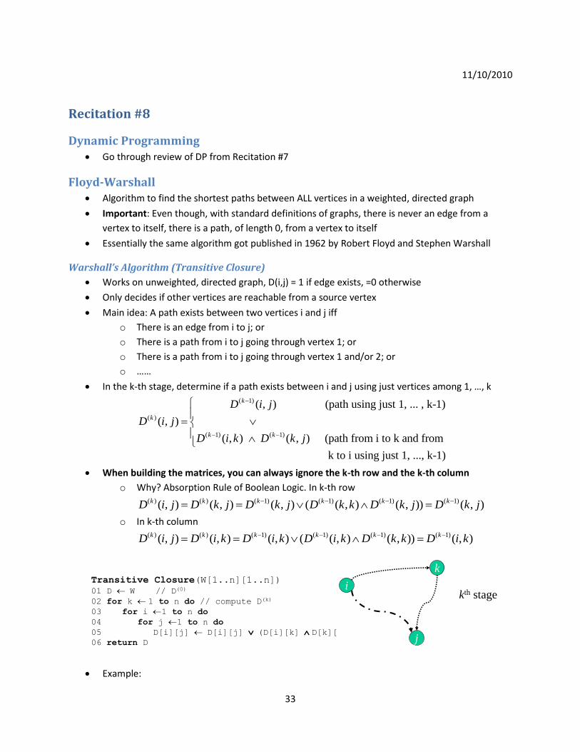
11/10/2010
Recitation #8
Dynamic Programming Go through review of DP from Recitation #7
Floyd-Warshall Algorithm to find the shortest paths between ALL vertices in a weighted, directed graph
Important: Even though, with standard definitions of graphs, there is never an edge from a
vertex to itself, there is a path, of length 0, from a vertex to itself
Essentially the same algorithm got published in 1962 by Robert Floyd and Stephen Warshall
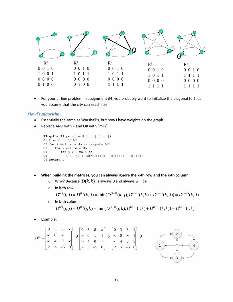
Warshall’s Algorithm (Transitive Closure)
Works on unweighted, directed graph, D(i,j) = 1 if edge exists, =0 otherwise
Only decides if other vertices are reachable from a source vertex
Main idea: A path exists between two vertices i and j iff
o There is an edge from i to j; or
o There is a path from i to j going through vertex 1; or
o There is a path from i to j going through vertex 1 and/or 2; or
o ……
In the k-th stage, determine if a path exists between i and j using just vertices among 1, …, k ( 1)
( )
( 1) ( 1)
( , ) (path using just 1, ... , k-1)
( , )
( , ) ( , ) (path from i to k and from
k to i using just 1, ..., k-1)
k
k
k k
D i j
D i j
D i k D k j
When building the matrices, you can always ignore the k-th row and the k-th column
o Why? Absorption Rule of Boolean Logic. In k-th row ( ) ( ) ( 1) ( 1) ( 1) ( 1)( , ) ( , ) ( , ) ( ( , ) ( , )) ( , )k k k k k kD i j D k j D k j D k k D k j D k j
o In k-th column ( ) ( ) ( 1) ( 1) ( 1) ( 1)( , ) ( , ) ( , ) ( ( , ) ( , )) ( , )k k k k k kD i j D i k D i k D i k D k k D i k
Example:
Transitive Closure(W[1..n][1..n])
01 D W // D(0)
02 for k 1 to n do // compute D(k)
03 for i 1 to n do
04 for j 1 to n do
05 D[i][j] D[i][j] (D[i][k] D[k][j])
06 return D
i
j
k
kth stage
34
For your airline problem in assignment #4, you probably want to initialize the diagonal to 1, as
you assume that the city can reach itself
Floyd’s Algorithm
Essentially the same as Warshall’s, but now I have weights on the graph
Replace AND with + and OR with “min”
When building the matrices, you can always ignore the k-th row and the k-th column
o Why? Because ( , )D k k is always 0 and always will be
o In k-th row ( ) ( ) ( 1) ( 1) ( 1) ( 1)( , ) ( , ) min( ( , ), ( , ) ( , )) ( , )k k k k k kD i j D k j D k j D k k D k j D k j
o In k-th column ( ) ( ) ( 1) ( 1) ( 1) ( 1)( , ) ( , ) min( ( , ), ( , ) ( , )) ( , )k k k k k kD i j D i k D i k D i k D k k D i k
Example:
(0)
0 3 8
0 1
4 0
2 5 0
D
5
0 3 8
0 1
4 0
2 5 0
0 3 8
0 1
4 0
2 5
4
0
5
5
3
42
1
3
42
13
42
1
3
42
1
R0
0 0 1 0
1 0 0 1
0 0 0 0
0 1 0 0
R1
0 0 1 0
1 0 1 1
0 0 0 0
0 1 0 0
R2
0 0 1 0
1 0 1 1
0 0 0 0
1 1 1 1
R3
0 0 1 0
1 0 1 1
0 0 0 0
1 1 1 1
R4
0 0 1 0
1 1 1 1
0 0 0 0
1 1 1 1
3
42
1
Floyd’s Algorithm(W[1..n][1..n])
01 D W // D(0)
02 for k 1 to n do // compute D(k)
03 for i 1 to n do
04 for j 1 to n do
05 D[i][j] MIND[i][j], D[i][k] + D[k][j])
06 return D
1 4
3
23 1
-58
4
2
35
0 3 8 4
0 1
4 0 5
2 5 01
0 3 4
0 1
4 0 5
2 1 5 0
1
3 4
7
Floyd-Warshall – Path Reconstruction
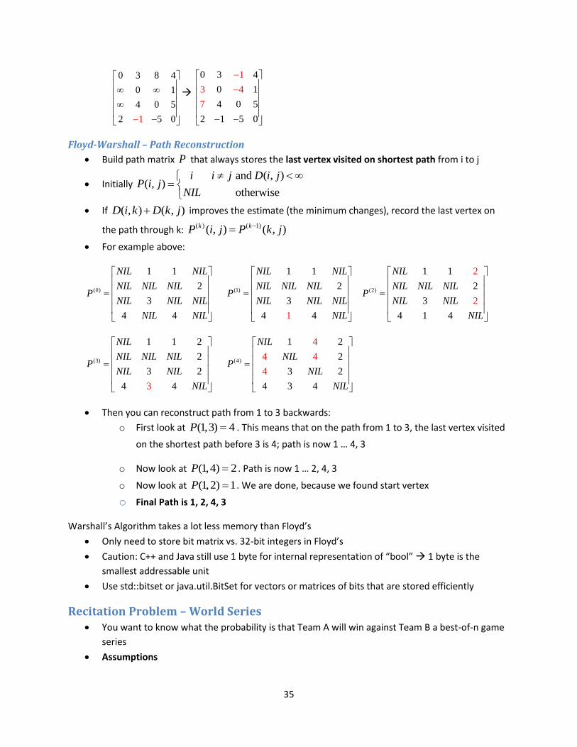
Build path matrix P that always stores the last vertex visited on shortest path from i to j
Initially and ( , )
( , )otherwise
i i j D i jP i j
NIL
If ( , ) ( , )D i k D k j improves the estimate (the minimum changes), record the last vertex on
the path through k: ( ) ( 1)( , ) ( , )k kP i j P k j
For example above:
(0)
1 1
2
3
4 4
NIL NIL
NIL NIL NILP
NIL NIL NIL
NIL NIL
(1)
1 1
2
3
14 4
NIL NIL
NIL NIL NILP
NIL NIL NIL
NIL
(2)
1 21
2
3
4 1 4
2
NIL
NIL NIL NILP
NIL NIL
NIL
(3)
1 1 2
2
3 2
4 43
NIL
NIL NIL NILP
NIL NIL
NIL
(4)
4
4
1 2
2
3 2
4 3 4
4
4
NIL
NILP
NIL
NIL
Then you can reconstruct path from 1 to 3 backwards:
o First look at (1,3) 4P . This means that on the path from 1 to 3, the last vertex visited
on the shortest path before 3 is 4; path is now 1 … 4, 3
o Now look at (1,4) 2P . Path is now 1 … 2, 4, 3
o Now look at (1,2) 1P . We are done, because we found start vertex
o Final Path is 1, 2, 4, 3
Warshall’s Algorithm takes a lot less memory than Floyd’s
Only need to store bit matrix vs. 32-bit integers in Floyd’s
Caution: C++ and Java still use 1 byte for internal representation of “bool” 1 byte is the
smallest addressable unit
Use std::bitset or java.util.BitSet for vectors or matrices of bits that are stored efficiently
Recitation Problem – World Series You want to know what the probability is that Team A will win against Team B a best-of-n game
series
Assumptions
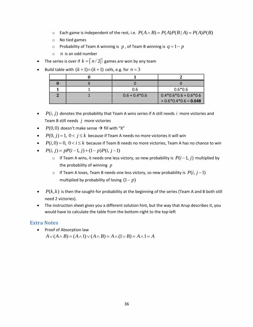
36
o Each game is independent of the rest, i.e. ( ) ( ) ( | ) ( ) ( )P A B P A P B A P A P B
o No tied games
o Probability of Team A winning is p , of Team B winning is 1q p
o n is an odd number
The series is over if / 2k n games are won by any team
Build table with ( 1) ( 1)k k cells, e.g. for 3n
0 1 2
0 X 0 0
1 1 0.6 0.6*0.6
2 1 0.6 + 0.4*0.6 0.4*0.6*0.6 + 0.6*0.6 + 0.6*0.4*0.6 = 0.648
( , )P i j denotes the probability that Team A wins series if A still needs i more victories and
Team B still needs j more victories
(0,0)P doesn’t make sense fill with “X”
(0, ) 1, 0P j j k because if Team A needs no more victories it will win
( ,0) 0, 0P i i k because if Team B needs no more victories, Team A has no chance to win
( , ) ( 1, ) (1 ) ( , 1)P i j pP i j p P i j
o If Team A wins, it needs one less victory, so new probability is ( 1, )P i j multiplied by
the probability of winning p
o If Team A loses, Team B needs one less victory, so new probability is ( , 1)P i j
multiplied by probability of losing (1 )p
( , )P k k is then the sought-for probability at the beginning of the series (Team A and B both still
need 2 victories).
The instruction sheet gives you a different solution hint, but the way that Arup describes it, you
would have to calculate the table from the bottom-right to the top-left
Extra Notes
Proof of Absorption law
( ) ( 1) ( ) (1 ) 1A A B A A B A B A A
37
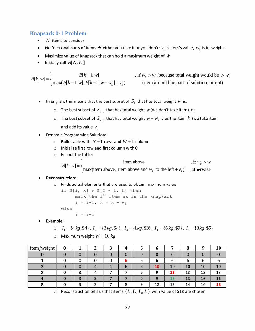
Knapsack 0-1 Problem
N items to consider
No fractional parts of items either you take it or you don’t; iv is item’s value, iw is its weight
Maximize value of Knapsack that can hold a maximum weight of W
Initially call [ , ]B N W
[ 1, ] , if (because total weight would be )[ , ]
max( [ 1, ], [ 1, ] ) (item could be part of solution, or not)
k
k k
B k w w w wB k w
B k w B k w w v k
In English, this means that the best subset of kS that has total weight w is:
o The best subset of 1kS that has total weight w (we don’t take item), or
o The best subset of 1kS that has total weight kw w plus the item k (we take item
and add its value kv
Dynamic Programming Solution:
o Build table with 1N rows and 1W columns
o Initialize first row and first column with 0
o Fill out the table:
item above , if [ , ]
max(item above, item above and to the left ) ,otherwise
k
k k
w wB k w
w v
Reconstruction:
o Finds actual elements that are used to obtain maximum value
if B[i, k] ≠ B[I - 1, k] then
mark the ith item as in the knapsack
i = i-1, k = k - wi
else
i = i-1
Example:
o 1 {4 ,$4}I kg , 2 {2 ,$4}I kg , 3 {1 ,$3}I kg , 4 {6 ,$9}I kg , 5 {3 ,$5}I kg
o Maximum weight 10W kg
item/weight 0 1 2 3 4 5 6 7 8 9 10
0 0 0 0 0 0 0 0 0 0 0 0
1 0 0 0 0 6 6 6 6 6 6 6
2 0 0 4 4 6 6 10 10 10 10 10
3 0 3 4 7 7 9 9 13 13 13 13
4 0 3 3 7 7 9 9 13 13 16 16
5 0 3 3 7 8 9 12 13 14 16 18
o Reconstruction tells us that items 1 2 3 5{ , , , }I I I I with value of $18 are chosen
38
11/17/2010
Recitation #9
Backtracking Clever implementation of exhaustive search
Incrementally builds candidates to the solutions, and abandons each partial candidate c
(“backtracks”) as soon as it determines that c cannot possibly be completed to a valid solution
Analogy of depth-first building a decision tree, each time you backtrack, you are basically
saying that a whole branch of a tree can be disregarded, because all decisions that happen in
there cannot possibly lead to a correct solution
Can be only applied for problems that have the concept of “partial candidate solution” and a
relatively quick test of whether it can possibly be completed to a valid solution
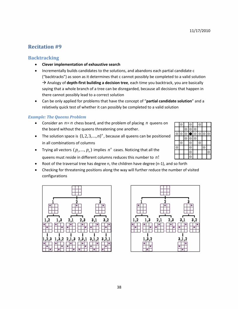
Example: The Queens Problem
Consider an n n chess board, and the problem of placing n queens on
the board without the queens threatening one another.
The solution space is {1,2,3,..., }nn , because all queens can be positioned
in all combinations of columns
Trying all vectors 1( ,..., )np p implies nn cases. Noticing that all the
queens must reside in different columns reduces this number to !n
Root of the traversal tree has degree n, the children have degree (n-1), and so forth
Checking for threatening positions along the way will further reduce the number of visited
configurations

39
Assignment #5 – Tentaizu Backtracking Japanese game that is basically Minesweeper, but you don’t get any redundant queues about
where mines are
The game is played on a 7x7 board. Exactly 10 of the 49 squares are each hiding a star.
Your task is to find the squares containing the 10 hidden stars.
You are guaranteed that each given Tentaizu board will have a unique solution.
Board B is two-dimensional array using some convention, e.g.:
1 for empty spot
( , ) [1,8] for star hint
9 for cells containing star
B x y
Build secondary array C that keeps track of which surrounding cells put a possible dependency
on a given cell
Table 1: Left: Board B (-1 cells are omitted for clarity); Right: Auxiliary Array C
1 3
1 0
2
3 3
1
1 1
Explanation of steps for function FIND-STAR(x,y)
1. For all cells in the table starting at position (x,y)
2. If all stars are placed and all cells in B have a value less or equal to 0, return true.
3. If we reach beyond the last cell of the table, we couldn’t place all stars, return
false.
4. Don’t try to put a star in any of the hint locations. Continue.
5. If this cell has no dependencies, we don’t know anything, so continue.
6. Make sure that we don’t violate any constraints of number of stars in B if we
would place a star here. If we do, continue.
7. Assume we can place a star. Decrement all hint cells that the current cell
depends on.
8. Run FIND-STAR again on the current position. If it returns true, return true.
9. Well, that didn’t work out. Set current cell back to BLANK and increment all
dependencies in B.
1 (0,0) (5,0) 3 (5,0)
(0,0) (1,2)
(0,0) (1,2)
(1,2) (4,2) (5,0) (4,2)
(5,0) (4,2)
(5,0)
(1,2) 1 (1,2) (3,3)
(4,2) (3,3) 0 (4,2)
(1,2) (1,4)
(1,2) (1,4)
(1,2) (3,3) (1,4)
2 (4,2) (3,3)
(4,2) (6,4)
(6,4)
(1,4) 3 (3,3) (1,4)
(3,3) (4,5)
(3,3) (4,5)
(6,4) (4,5) 3
(1,4) (1,4) (1,4) (3,6)
(4,5) (3,6) 1
(6,4) (4,5) (6,6)
(6,4) (6,6)
(3,6) 1 (4,5) (3,6)
(4,5) (6,6) 1
40
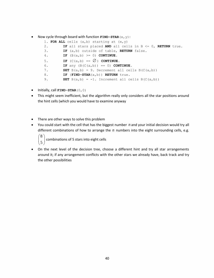
Now cycle through board with function FIND-STAR(x,y): 1. FOR ALL cells (a,b) starting at (x,y)
2. IF all stars placed AND all cells in B <= 0, RETURN true.
3. IF (a,b) outside of table, RETURN false.
4. IF (B(a,b) >= 0) CONTINUE.
5. IF (C(a,b) == ) CONTINUE.
6. IF any (B(C(a,b)) == 0) CONTINUE.
7. SET B(a,b) = 9. Decrement all cells B(C(a,b))
8. IF (FIND-STAR(a,b)) RETURN true.
9. SET B(a,b) = -1. Increment all cells B(C(a,b))
Initially, call FIND-STAR(0,0)
This might seem inefficient, but the algorithm really only considers all the star positions around
the hint cells (which you would have to examine anyway
There are other ways to solve this problem
You could start with the cell that has the biggest number n and your initial decision would try all
different combinations of how to arrange the n numbers into the eight surrounding cells, e.g.
8
5
combinations of 5 stars into eight cells
On the next level of the decision tree, choose a different hint and try all star arrangements
around it; if any arrangement conflicts with the other stars we already have, back track and try
the other possibilities

41
Lab Problem – Robot Path Finding A robot is placed in an n n maze at starting position (1,0) in the maze and is asked to try to
reach the right side (if there is a path to ( 1, )n y where y is any number between 0 and 1n
At any given moment, the robot can only move 1 step
in one of 4 directions:
o Go North: ( , ) ( , 1)x y x y
o Go East : ( , ) ( 1, )x y x y
o Go South : ( , ) ( , 1)x y x y
o Go West : ( , ) ( 1, )x y x y
Solve the path using recursion with FIND-PATH
function:
FIND-PATH(x, y)
1. if (x,y outside maze) return false 2. if (x,y already visited) return
false
3. if (x,y not open) return false 4. if (x,y is goal) return true 5. if (FIND-PATH(North of x,y) ==
true) return true
6. if (FIND-PATH(East of x,y) == true) return true
7. if (FIND-PATH(South of x,y) == true) return true
8. if (FIND-PATH(West of x,y) == true) return true
9. return false
Initially, call FIND-PATH(1, 0)
Note, that if a path to the goal was found, it is
important that the algorithm stops, i.e., if going North
of x, y finds a path (i.e., returns true), then from the
current position (i.e., current call of FIND-PATH) there
is no need to check East, South or West. Instead, FIND-
PATH just need return true to the previous call.
Backtracking happens automatically through nature of
recursion, because it keeps track of the tried paths
It will find the path, if one exists (although not
necessarily the shortest one) It’s almost like a depth-
first search of the maze from your starting position
42
12/01/2010
Exam Review - Final
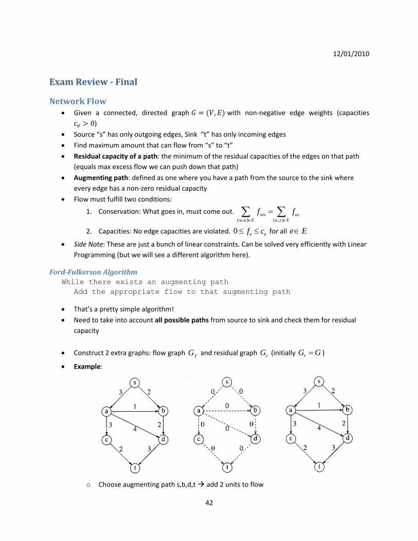
Network Flow Given a connected, directed graph ( ) with non-negative edge weights (capacities
)
Source “s” has only outgoing edges, Sink “t” has only incoming edges
Find maximum amount that can flow from “s” to “t”
Residual capacity of a path: the minimum of the residual capacities of the edges on that path
(equals max excess flow we can push down that path)
Augmenting path: defined as one where you have a path from the source to the sink where
every edge has a non-zero residual capacity
Flow must fulfill two conditions:
1. Conservation: What goes in, must come out. ( , ) ( , )
wu uz
w u E u z E
f f
2. Capacities: No edge capacities are violated. 0 e ef c for all e E
Side Note: These are just a bunch of linear constraints. Can be solved very efficiently with Linear
Programming (but we will see a different algorithm here).
Ford-Fulkerson Algorithm
While there exists an augmenting path
Add the appropriate flow to that augmenting path
That’s a pretty simple algorithm!
Need to take into account all possible paths from source to sink and check them for residual
capacity
Construct 2 extra graphs: flow graph fG and residual graph rG (initially rG G )
Example:
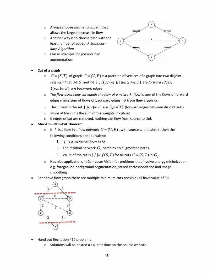
o Choose augmenting path s,b,d,t add 2 units to flow

43
o Choose augmenting path s,a,c,t add 2 units of flow
o Choose augmenting path s,a,d,t add 1 unit of flow
o Algorithm terminates, because t is unreachable from s.
o Resulting maximum flow is 5
Problem:
o What happens if we choose a different first path?
o Choose augmenting path s,a,d,t add 3 units to flow
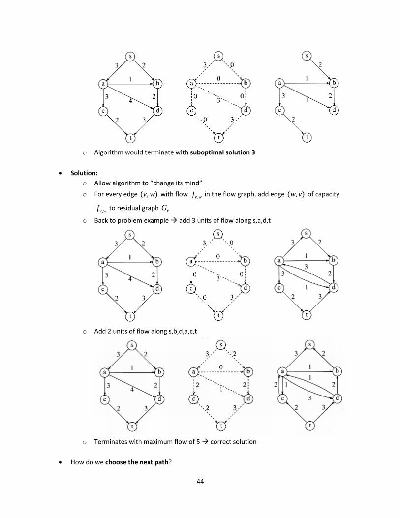
44
o Algorithm would terminate with suboptimal solution 3
Solution:
o Allow algorithm to “change its mind”
o For every edge ( , )v w with flow ,v wf in the flow graph, add edge ( , )w v of capacity
,v wf to residual graph rG
o Back to problem example add 3 units of flow along s,a,d,t
o Add 2 units of flow along s,b,d,a,c,t
o Terminates with maximum flow of 5 correct solution
How do we choose the next path?
45
o Always choose augmenting path that
allows the largest increase in flow
o Another way is to choose path with the
least number of edges Edmonds-
Karp Algorithm
o Classic example for possible bad
augmentation:
Cut of a graph
o ( , )C S T of graph ( , )G V E Is a partition of vertices of a graph into two disjoint
sets such that s S and t T ; {( , ) | , }u v E u S v T are forward edges;
{( , ) }v u E are backward edges
o The flow across any cut equals the flow of a network.(flow is sum of the flows of forward
edges minus sum of flows of backward edges) from flow graph fG
o The cut-set is the set {( , ) | , }u v E u S v T (forward edges between disjoint sets)
o Value of the cut is the sum of the weights in cut-set
o If edges of cut are removed, nothing can flow from source to sink
Max-Flow Min-Cut Theorem
o If f is a flow in a flow network ( , )G V E , with source s and sink t , then the
following conditions are equivalent:
1. f is a maximum flow in G
2. The residual network rG contains no augmented paths.
3. Value of the cut is | | ( , )f f S T for all cuts ( , )C S T in fG .
o Has nice applications in Computer Vision for problems that involve energy minimization,
e.g. foreground-background segmentation, stereo correspondence and image
smoothing
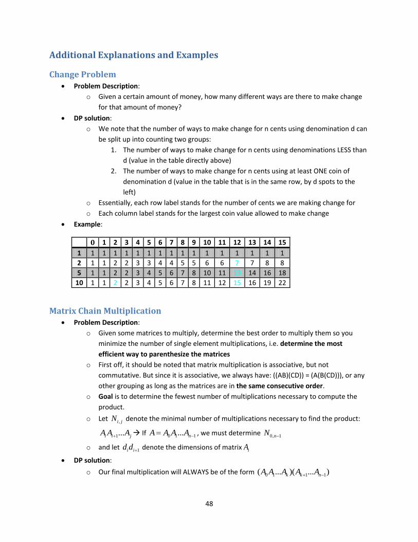
For above flow graph there are multiple minimum cuts possible (all have value of 5):
Hand out Recitation #10 problems
o Solutions will be posted a t a later time on the course website

46
o Discuss possible solution for problem 1
o Problem 2 is the optional homework problem
o Problem 3 is verbatim from slides
47
More Final Exam Review You can have 3 sheets of letter-sized paper filled on both sides, so don’t waste your time
remembering definitions or lengthy proofs
The following sections list the topics that weren’t covered in Exam 1 & 2 and that Sarah
mentioned in her topics list
Dynamic Programming Change Problem see following pages
Floyd-Warshall's Algorithm and path reconstruction Recitation #8; additional example on
review sheet
Transitive Closure Recitation #8; additional example there
Longest Common Subsequence Recitation #7; additional example on review sheet
Edit Distance Recitation #7; additional example on review sheet
Knapsack 0-1 Problem Recitation #8; additional example on review sheet
Matrix Chain Multiplication see following pages; additional example on review sheet
World Series Problem Recitation #8 problem; additional example below
Backtracking Eight Queens Recitation #9; additional example on review sheet
Magic Square additional example on review sheet
Sudoku See following pages
Tentaizu Assignment #5, see explanation in recitation #9
Network Flow Maximum Flow Today’s material; additional example above
Minimum Cut Today’s material; additional example above
Use of BFS
Bipartite Matching Sarah hasn’t covered that yet
Matching Instructors to classes Today’s material
Filling an orchestra, etc. Today’s material
48
Additional Explanations and Examples
Change Problem
Problem Description:
o Given a certain amount of money, how many different ways are there to make change
for that amount of money?
DP solution:
o We note that the number of ways to make change for n cents using denomination d can
be split up into counting two groups:
1. The number of ways to make change for n cents using denominations LESS than
d (value in the table directly above)
2. The number of ways to make change for n cents using at least ONE coin of
denomination d (value in the table that is in the same row, by d spots to the
left)
o Essentially, each row label stands for the number of cents we are making change for
o Each column label stands for the largest coin value allowed to make change
Example:
0 1 2 3 4 5 6 7 8 9 10 11 12 13 14 15
1 1 1 1 1 1 1 1 1 1 1 1 1 1 1 1 1
2 1 1 2 2 3 3 4 4 5 5 6 6 7 7 8 8
5 1 1 2 2 3 4 5 6 7 8 10 11 13 14 16 18
10 1 1 2 2 3 4 5 6 7 8 11 12 15 16 19 22
Matrix Chain Multiplication Problem Description:
o Given some matrices to multiply, determine the best order to multiply them so you
minimize the number of single element multiplications, i.e. determine the most
efficient way to parenthesize the matrices
o First off, it should be noted that matrix multiplication is associative, but not
commutative. But since it is associative, we always have: ((AB)(CD)) = (A(B(CD))), or any
other grouping as long as the matrices are in the same consecutive order.
o Goal is to determine the fewest number of multiplications necessary to compute the
product.
o Let ,i jN denote the minimal number of multiplications necessary to find the product:
1...i i jA A A If 0 1 1... nA A A A , we must determine 0, 1nN
o and let 1i id d denote the dimensions of matrix iA
DP solution:
o Our final multiplication will ALWAYS be of the form 0 1 1 1( ... )( ... )k k nA A A A A
49
o In essence, there is exactly one value of k for which we should "split" our work into two
separate cases so that we get an optimal result
o Count the number of multiplications in each of these choices and pick the minimum
o Recursive formula:
, , 1, 1 1valid values of (min( ))i j i k k j i k jN k N N d d d Look at all possible ways
to split multiplication
o Build table Initialize diagonal to 0 and all other entries to
o Order of filling N matrix:
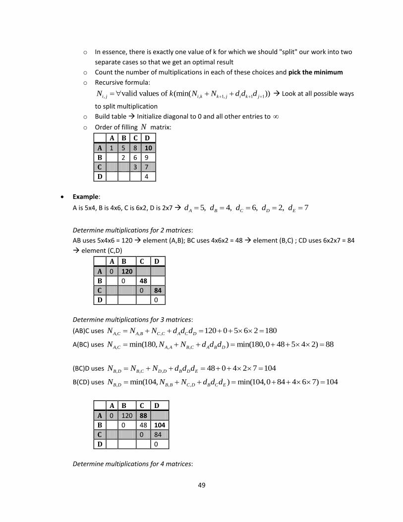
A B C D
A 1 5 8 10
B 2 6 9
C 3 7
D 4
Example:
A is 5x4, B is 4x6, C is 6x2, D is 2x7 5, 4, 6, 2, 7A B C D Ed d d d d
Determine multiplications for 2 matrices:
AB uses 5x4x6 = 120 element (A,B); BC uses 4x6x2 = 48 element (B,C) ; CD uses 6x2x7 = 84
element (C,D)
A B C D
A 0 120
B 0 48
C 0 84
D 0
Determine multiplications for 3 matrices:
(AB)C uses , , , 120 0 5 6 2 180A C A B C C A C DN N N d d d
A(BC) uses , , ,min(180, ) min(180,0 48 5 4 2) 88A C A A B C A B DN N N d d d
(BC)D uses , , , 48 0 4 2 7 104B D B C D D B D EN N N d d d
B(CD) uses , , ,min(104, ) min(104,0 84 4 6 7) 104B D B B C D B C EN N N d d d
A B C D
A 0 120 88
B 0 48 104
C 0 84
D 0
Determine multiplications for 4 matrices:
50
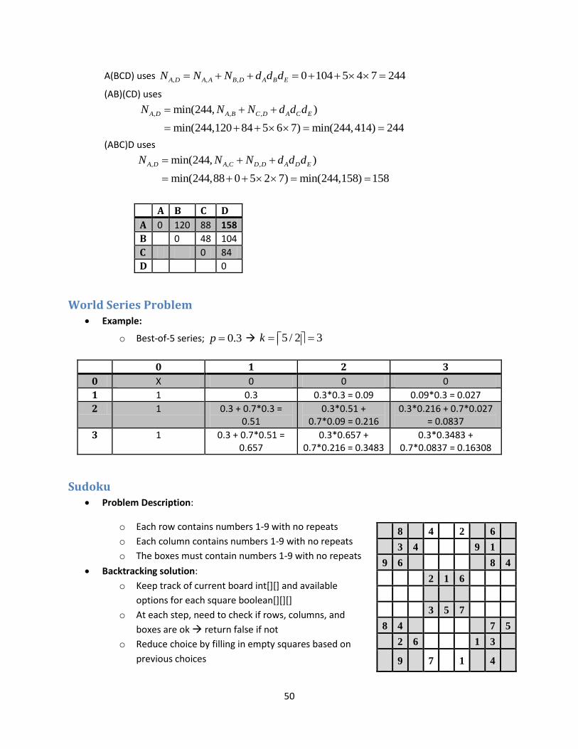
A(BCD) uses , , , 0 104 5 4 7 244A D A A B D A B EN N N d d d
(AB)(CD) uses
, , ,min(244, )
min(244,120 84 5 6 7) min(244,414) 244
A D A B C D A C EN N N d d d
(ABC)D uses
, , ,min(244, )
min(244,88 0 5 2 7) min(244,158) 158
A D A C D D A D EN N N d d d
A B C D
A 0 120 88 158
B 0 48 104
C 0 84
D 0
World Series Problem Example:
o Best-of-5 series; 0.3p 5 / 2 3k
0 1 2 3
0 X 0 0 0
1 1 0.3 0.3*0.3 = 0.09 0.09*0.3 = 0.027
2 1 0.3 + 0.7*0.3 = 0.51
0.3*0.51 + 0.7*0.09 = 0.216
0.3*0.216 + 0.7*0.027 = 0.0837
3 1 0.3 + 0.7*0.51 = 0.657
0.3*0.657 + 0.7*0.216 = 0.3483
0.3*0.3483 + 0.7*0.0837 = 0.16308
Sudoku Problem Description:
o Each row contains numbers 1-9 with no repeats
o Each column contains numbers 1-9 with no repeats
o The boxes must contain numbers 1-9 with no repeats
Backtracking solution:
o Keep track of current board int[][] and available
options for each square boolean[][][]
o At each step, need to check if rows, columns, and
boxes are ok return false if not
o Reduce choice by filling in empty squares based on
previous choices
8
4
2
6
3 4
9 1
9 6
8 4
2 1 6
3 5 7
8 4
7 5
2 6
1 3
9
7
1
4


![Java Programming [Individual Assignment]](https://img.pdfslide.net/doc/110x75/5521765e4979597f2f8b54fb/java-programming-individual-assignment.jpg)
