Embed Size (px)
Citation preview
8/13/2019 Lab Textbook (Partial)
http://slidepdf.com/reader/full/lab-textbook-partial 1/68
Measurement and Instrumentation Lab #1: Intro and Resistor Statistics
Page 1
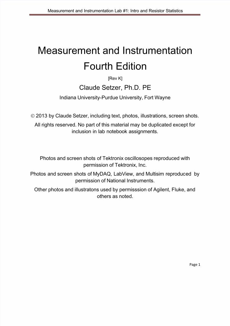
Measurement and InstrumentationFourth Edition
[Rev K] Claude Setzer, Ph.D. PE
Indiana University-Purdue University, Fort Wayne
2013 by Claude Setzer, including text, photos, illustrations, screen shots.
All rights reserved. No part of this material may be duplicated except for
inclusion in lab notebook assignments.
Photos and screen shots of Tektronix oscillosopes reproduced with
permission of Tektronix, Inc.Photos and screen shots of MyDAQ, LabView, and Multisim reproduced by
permission of National Instruments.
Other photos and illustratons used by permisssion of Agilent, Fluke, and
others as noted.
8/13/2019 Lab Textbook (Partial)
http://slidepdf.com/reader/full/lab-textbook-partial 2/68
Measurement and Instrumentation Lab #1: Intro and Resistor Statistics
Page 2
List of Lab Topics:1. LabVIEW, Statistics of Resistors, and Uncertainty Analysis [DMM and LabVIEW]
2. System Loading [Analog and Digital multimeters]
3. Oscilloscope Calibration [Digital Scope, Freq. counter, Signal Generator]
4. Low Pass Filter, Forced Response/Natural Response,[manual measurement]5. Natural Frequency, RLC Frequency Response. [Scope, Signal Generator]
6. Natural Response (RLC Step Response) [Scope, Signal Generator]
7. Bode Plots [series RLC automated measurements using MyDAQ]
8. RC Bode Diagram [automated measurements using MyDAQ]
9. Active Filters One: First Order Low Pass Filter. [Multisim Simulation]
10. Factory simulation, 2nd and 3rd Order Low Pass Filter, [Multisim]
11. OpAMP Applications: LED Traffic Light [Multisim]
12. ELVIS Pressure Measurement/Calibration [Piezoelectric Sensor, MyDAQ DMM]
13. Signal Conditioning Amplifier [OpAmp, MyDAQ Automated Measurements]
14. Pressure Sensor [LabVIEW with DAQ simulation]15. Factory Protection: Pressure Sensor Measurements [MyDAQ A/D input]
16. Thermocouple Simulation and Measurement [LabVIEW and My DAQ]
17. Thermocouple Calibration [use Lab 16 setup, calibrate to freezing water +]
18. Lean Manufacturing [CNC design, fabrication, and measurements]
19. Lab Standards + Quiz
20. Motor Speed [Square wave generator in LabVIEW to simulate LED pulses]
21. Motor Speed Measurements [Amplified LED pulses into MyDAQ/LabVIEW]
22. Lab Safety + Quiz
23. Strain Gauge Simulation [Signal Simulation VI in LabVIEW]24. Strain Gauge Calibration [Wheatstone Bridge output to MyDAQ DMM, cal. block]
25. Vacuum Systems + Quiz
26. Vacuum Gauge [LabVIEW Thermocouple gauge measurement simulation]
27. Measurement of Mechanical Vibration [Laser Position Sensor + LabVIEW]
Index
You will be given needed help on how to do many specific activities, but you are
expected to basically Design (your own) Experiment to demonstrate each topic, and then
to describe details of your design, including formal Uncertaitny Analysis.
8/13/2019 Lab Textbook (Partial)
http://slidepdf.com/reader/full/lab-textbook-partial 3/68
Measurement and Instrumentation Lab #1: Intro and Resistor Statistics
Page 3
Course Overview
Design of Experiments
Design is widely considered to be the essence of effective engineering . In its
most general and deepest aspect, as described by ABET, the design process is creativeand open–ended, with consideration for the holistic nature of the project in question,
and with no single or uniquely “best” outcome. It does, however, require careful andclearly defined process and often includes a variety of pre – specified requirements.The process, and to some extent the methodology for creativity, can be taught, but
these are largely developed by experience.
This is the overall goal of this course, to help you learn the DESIGN process, both
through methodology and through experience.
If learned well, this skill will become the foundation for all of your future work as an
engineering professional. Being successful is NOT something the teacher can do foryou => you must be personally engaged in the process. You should not expectevery detail to be given to you, but you need to THINK about how to do things in orderto get the required result in the best possible way.
This is NOT a “circuit design” course and you will not be expected to independentlydesign and/or build circuits. You will be expected to understand how the circuit designprocess/procedure was used to implement some of the circuits you will use.
Design of Experiments, at least as used in this course, refers to planning the labexperiment so that the required outcome can be accomplished. Among other things,this means considering specifications (including numbers !) and needed measure–
ments BEFORE starting the lab/experiment.Structure of this Course
A typical 1- unit engineering lab course at most universities in the US would includeeither 3 or 4 hours of lab time once per week, along with 1 or 2 hours outside of lab timefor each hour in lab. There would be 15 to 16 labs per semester. This course is anintegrated combination of two courses that would normally have 30 or moreassociated lab sessions and sometimes also a final exam.
Integration of the two courses has allowed substantial savings in time andefficiency, while enhancing your learning experience:
1. The number of lab sessions has been reduced from over 30 down to about27, giving you several days of extra time with not lab or class.
2. There is no final exam.3. The emphasis is on experience.4. Course is tightly focused on most important skills and topics, with inclusion of
many topics directly linked to realistic industrial use of the skills taught.
Technical material in the course:
s s t e overa goa o t s course, to e p you earn t e DESIGN process, ot
t roug met o o ogy an t roug exper ence.
8/13/2019 Lab Textbook (Partial)
http://slidepdf.com/reader/full/lab-textbook-partial 4/68
Measurement and Instrumentation Lab #1: Intro and Resistor Statistics
Page 4
For more than a hundred years, engineering education has recognized andemphasized the interdependence of mechanical and electrical design (includingcomputer engineering). An engineering professional in any of these 3 areas is muchweaker and less effective without some background in the other two. Today, thisinterdependence has become even more critical, especially in the area of measurement
and instrumentation. From the viewpoint of a mechanical engineer, the purely“mechanical” measuring instrument is not only less effective and less accurate, butthere are literally not many left in use. From the viewpoint of electrical and computerengineers, the same type of need exists. For example, the major limit for performanceof many electronic systems is not the electronic portion, but the mechanical parts, suchas the physical endurance of a product or the ability to remove sufficient heat for theproduct to continue operation. Virtually all universities require mechanical engineers to atake a basic Circuits course and lab, while all require electrical and computer engineersare generally required to take basic mechanical engineering courses and labs. Someuniversities, like IPFW, enhance the experience of both by integrating them into one labcourse.
Lab Notebook: [NOT a Lab “REPORT”]
The initial reaction of many engineers is that the amount of writing required for aneffective lab notebook is somewhat of a “bother,” as Pooh would say. Successfulengineers soon discover, however, that the lab notebook is one of the most importantfoundations of their success. Taking notes in real time and recording all details, nomatter how unimportant or unforgettable they may seem at the time, is virtually the onlyway to insure 2 critical things: 1) that the data is not lost due to incorrect or inadequatememory, and 2) that the person who did the work has legal basis for getting properrecognition, such as a patent. A major goal of this course is to help you develop skillsin keeping an effective/complete engineering lab notebook.
Basic Circuits:
Filter circuits are the most widely used and important of all circuits, as they allow asystem to discriminate between desirable and undesirable results. The traditionallecture and lab course in basic circuits is typically a required background for allengineers. That course would include basic material of building and testing theproperties of basic passive circuits, typically using a few resistors, capacitors, andinductors, with values and configuration to support the needed Design of Experiments.The next higher level of circuits would be active circuits or “electronics,” in which manyvarieties of amplifiers and other processing circuits would be designed, built, and tested.In the more modern version of the traditional Circuits course, the basic coverage of
passive filters has been expanded to include Active Filters, reflecting the fact thatActive Filters have become part of almost every electronic system today. This coursewill introduce this modern implementation of including Active Filters, but will do it in asimple straight forward way that is equally accessible to all engineers without need for abackground in electronics. The amplifying element that will be used in the Active Filter isthe Operational Amplifier [OpAmp], an integrated circuit that allows high performancewhile using only a simple “cookbook” method for specifying details of its implementation.

8/13/2019 Lab Textbook (Partial)
http://slidepdf.com/reader/full/lab-textbook-partial 5/68
Measurement and Instrumentation Lab #1: Intro and Resistor Statistics
Page 5
Instrumentation:
You will learn how to use all of the basic instruments, both analog and digital, thatare traditionally used for measuring the properties of basic circuit elements and basiccircuits, including Active Filters.=> Signal Generator, Voltage and Current meters,
Oscilloscope, Frequency counter, digital data acquisition. In addition, you will learn touse some of the newest, most powerful, and perhaps most convenient, digitalprocessing instruments built into the MyDAQ system. All of these, plus an automatedBode Plotting system, are part of the digital capabilities of the LabView AutomatedMeasurement System, one of the most common and most powerful tools available forautomated measurements and signal processing.
Mechanical Engineering Measurements:
The vast majority of modern measurements are automated, which requires, by itsnature, that they be in electronic format, usually digital. Even in the “purely” mechanicalsystem, the purely mechanical measurement instrument has almost disappeared. The
process of design and analysis of any system requires the use ofideal models
that aretranslated back and forth with real physical systems. All computers and allmathematical equations use only ideal models and relate these models to a non-ideal physical system. In doing this, all systems, whether electrical, mechanical,chemical, or others, can be described and modeled by the same mathematicalequations and analyzed by the same computer programs.
This entire course is structured around mechanical engineeringmeasurements, and the circuit material is all developed with this focus. [Almosteverything could be taught in a similar way with electronic focus, physics focus,chemical focus computer focus and so on…] the starting point for a measurement isbasically a sensor or transducer– a device that translates some type of mechanical
activity into electrical activity, so that it can be captured and analyzed by a computer.The most important aspect of this measurement is the filtering component that can beeither a physical Active Filter used before the computer takes over, or a Digital Filter that is used after the computer takes over. Both have their advantages and both will beused in this course. Some of the mechanical sensors to be used are: thermocouple,piezoelectric transducer, strain gauge, LED transmitter/receiver, and Laser PositionSensor. There will also be experience of the fundamentals of Computer controlledmanufacturing process and the associated measurements.
Statistics
Every measurement has a statistical uncertainty component, and in many cases this
component is extremely important for determining the true significance of themeasurement. You will start the course by taking a representative statisticalmeasurement and compare one reading to 10 and 40 or 50 measurements. However, toactually have statistically significant measurements it can sometimes require 10s ofthousands of such measurements and become impractical. Thus, a good substitutehas been developed to achieve much of the quality of statistical measurements whilenot having to do them every time. Effectively, the manufacturer of each part does thethousands of required measurements and then adds a statistical component to the
8/13/2019 Lab Textbook (Partial)
http://slidepdf.com/reader/full/lab-textbook-partial 6/68
8/13/2019 Lab Textbook (Partial)
http://slidepdf.com/reader/full/lab-textbook-partial 7/68
Measurement and Instrumentation Lab #1: Intro and Resistor Statistics
Page 7
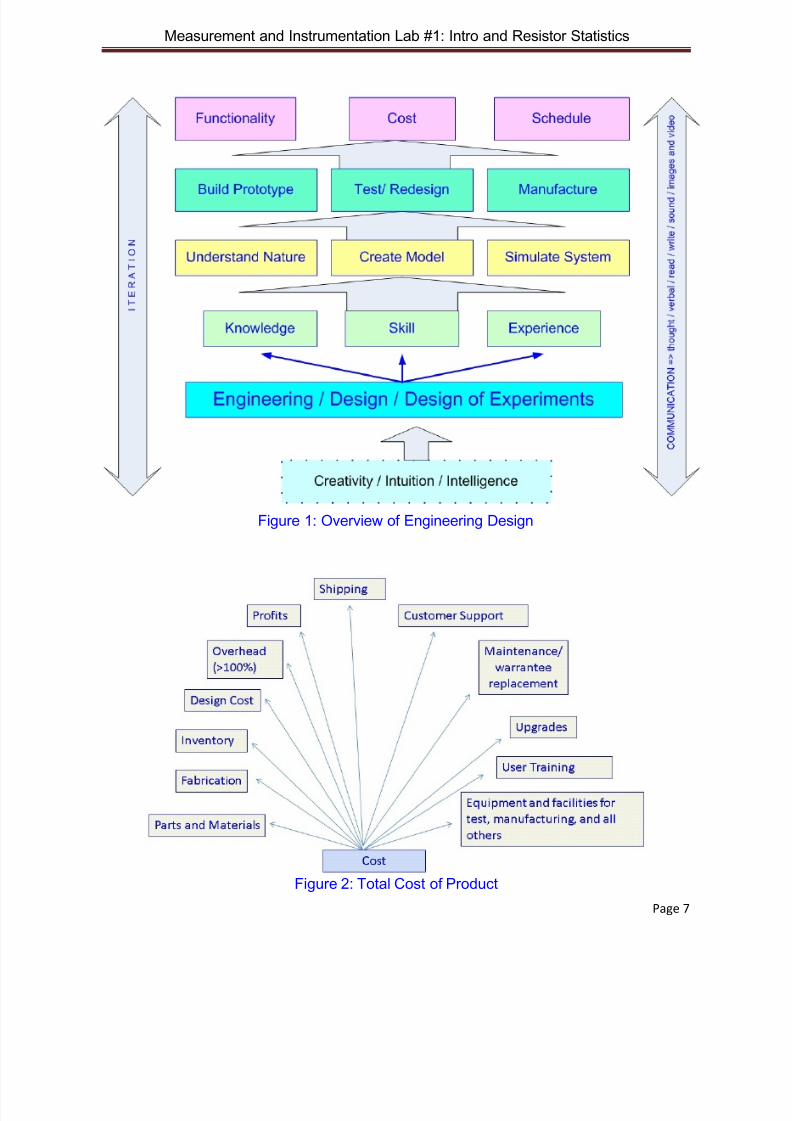
Figure 1: Overview of Engineering Design
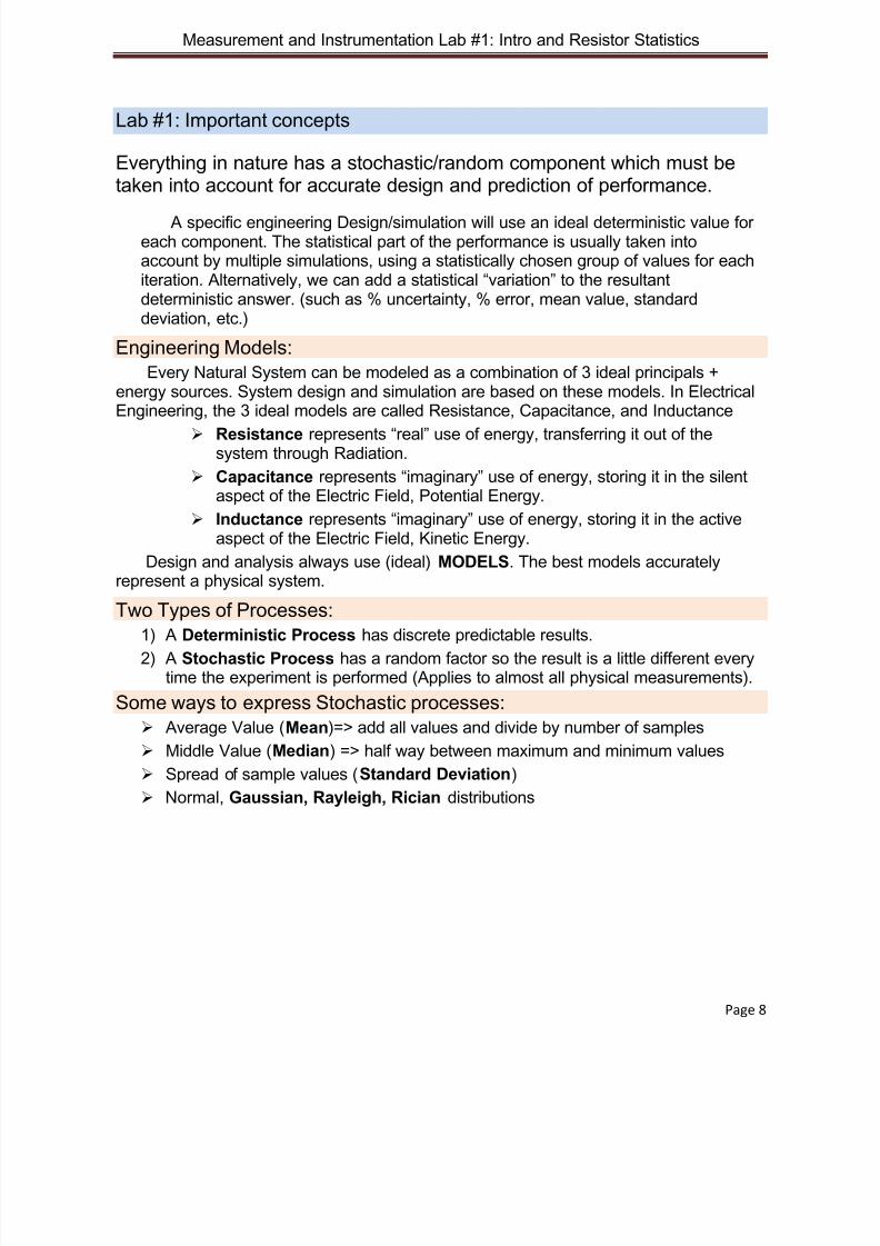
Figure 2: Total Cost of Product
8/13/2019 Lab Textbook (Partial)
http://slidepdf.com/reader/full/lab-textbook-partial 8/68
Measurement and Instrumentation Lab #1: Intro and Resistor Statistics
Page 8
Lab #1: Important concepts
Everything in nature has a stochastic/random component which must betaken into account for accurate design and prediction of performance.
A specific engineering Design/simulation will use an ideal deterministic value foreach component. The statistical part of the performance is usually taken intoaccount by multiple simulations, using a statistically chosen group of values for eachiteration. Alternatively, we can add a statistical “variation” to the resultantdeterministic answer. (such as % uncertainty, % error, mean value, standarddeviation, etc.)
Engineering Models:Every Natural System can be modeled as a combination of 3 ideal principals +
energy sources. System design and simulation are based on these models. In ElectricalEngineering, the 3 ideal models are called Resistance, Capacitance, and Inductance
Resistance represents “real” use of energy, transferring it out of thesystem through Radiation.
Capacitance represents “imaginary” use of energy, storing it in the silentaspect of the Electric Field, Potential Energy.
Inductance represents “imaginary” use of energy, storing it in the activeaspect of the Electric Field, Kinetic Energy.
Design and analysis always use (ideal) MODELS. The best models accuratelyrepresent a physical system.
Two Types of Processes:
1) A Deterministic Process has discrete predictable results.2) A Stochastic Process has a random factor so the result is a little different every
time the experiment is performed (Applies to almost all physical measurements).
Some ways to express Stochastic processes: Average Value (Mean)=> add all values and divide by number of samples
Middle Value (Median) => half way between maximum and minimum values
Spread of sample values (Standard Deviation)
Normal, Gaussian, Rayleigh, Rician distributions
8/13/2019 Lab Textbook (Partial)
http://slidepdf.com/reader/full/lab-textbook-partial 9/68
Measurement and Instrumentation Lab #1: Intro and Resistor Statistics
Page 9
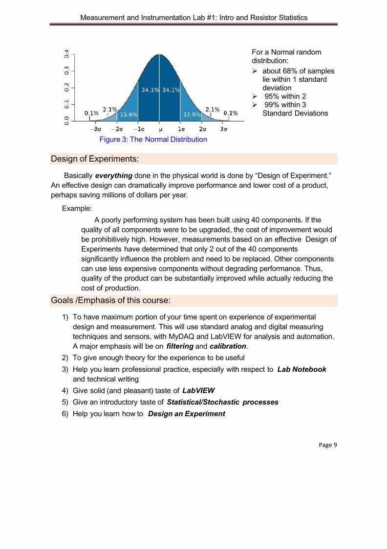
For a Normal randomdistribution:
about 68% of sampleslie within 1 standarddeviation
95% within 2 99% within 3
Standard Deviations
Figure 3: The Normal Distribution
Design of Experiments:
Basically everything done in the physical world is done by “Design of Experiment.”
An effective design can dramatically improve performance and lower cost of a product,perhaps saving millions of dollars per year.
Example:
A poorly performing system has been built using 40 components. If the
quality of all components were to be upgraded, the cost of improvement would
be prohibitively high. However, measurements based on an effective Design of
Experiments have determined that only 2 out of the 40 components
significantly influence the problem and need to be replaced. Other components
can use less expensive components without degrading performance. Thus,
quality of the product can be substantially improved while actually reducing thecost of production.
Goals /Emphasis of this course:
1) To have maximum portion of your time spent on experience of experimental
design and measurement. This will use standard analog and digital measuring
techniques and sensors, with MyDAQ and LabVIEW for analysis and automation.
A major emphasis will be on filtering and calibration.
2) To give enough theory for the experience to be useful
3) Help you learn professional practice, especially with respect to Lab Notebook
and technical writing
4) Give solid (and pleasant) taste of LabVIEW
5) Give an introductory taste of Statistical/Stochastic processes
6) Help you learn how to Design an Experiment
8/13/2019 Lab Textbook (Partial)
http://slidepdf.com/reader/full/lab-textbook-partial 10/68
Measurement and Instrumentation Lab #1: Intro and Resistor Statistics
Page 10
LabVIEW Tutorial:
The following tutorial will introduce some of the most basic functions of using the
LabVIEW “interface” to Digital Signal Processing. After this, the first lab session will be a
combination of physical measurements using a traditional digital multimeter and
LabVIEW to analyze the statistical nature of that data. After getting a taste of this directstatistical analysis, we will use a much more widespread type of statistical analysis that
makes use of a “shorthand” method.
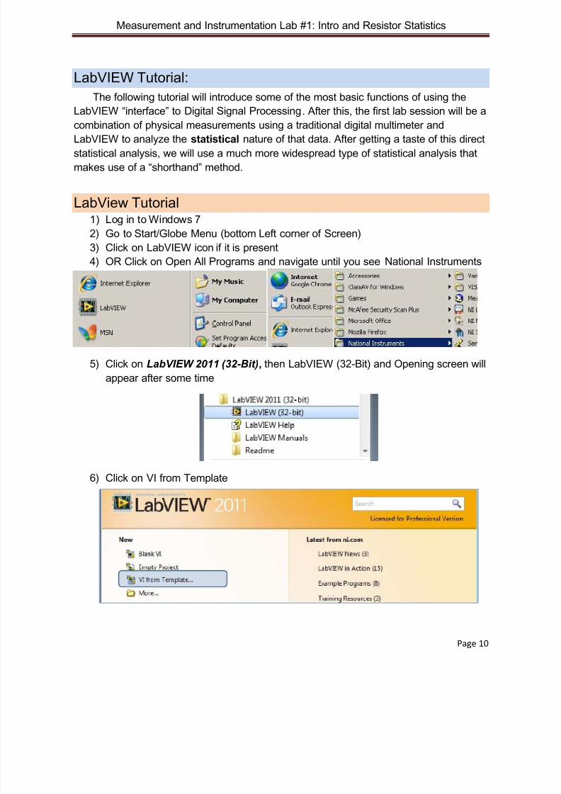
LabView Tutorial1) Log in to Windows 7
2) Go to Start/Globe Menu (bottom Left corner of Screen)
3) Click on LabVIEW icon if it is present
4) OR Click on Open All Programs and navigate until you see National Instruments
5) Click on LabVIEW 2011 (32-Bit), then LabVIEW (32-Bit) and Opening screen will
appear after some time
6) Click on VI from Template

8/13/2019 Lab Textbook (Partial)
http://slidepdf.com/reader/full/lab-textbook-partial 11/68
Measurement and Instrumentation Lab #1: Intro and Resistor Statistics
Page 11
7) Highlight Tutorial => Generate and Display, then click on OK.
Basic Operations:
LabVIEW normally opens with two windows, Front Panel and Block Diagram
1) If only one window is open, click on Window menu at top of screen and
then click on name of other window. Here Front Panel is present so click
on Show Block Diagram
2) It is very useful to also have the Tools menu open=> Click on View menu
at top of screen, then select Tools Palette. Move mouse over Tools icon
and click to change cursor function.
3) Both Front Panel and Block Diagram have an associated palette of
models or functions that can be added to that window. If these pallets arenot on the screen when a panel is selected, then add it in the same way:
For Front Panel , click on View menu at top, then on Controls Palette.
For Block Diagram, click on View menu and select Functions Palette,
the only one available. The icons may only be used when a given widow is
active. When Front Panel is active you can use the Controls Palette.
8/13/2019 Lab Textbook (Partial)
http://slidepdf.com/reader/full/lab-textbook-partial 12/68
Measurement and Instrumentation Lab #1: Intro and Resistor Statistics
Page 12
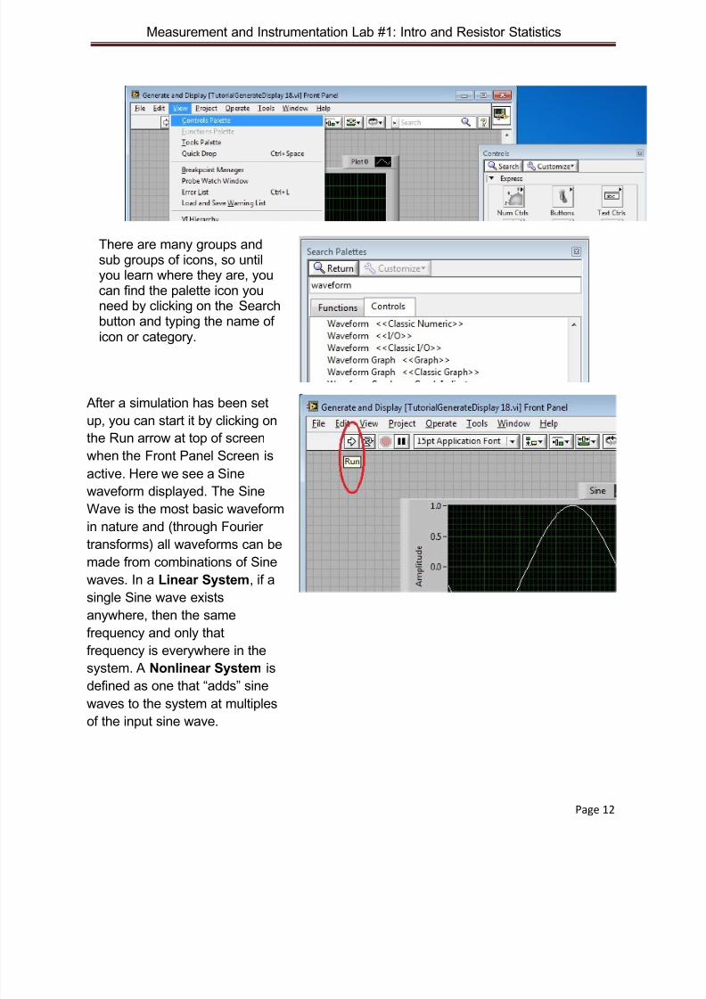
There are many groups andsub groups of icons, so untilyou learn where they are, youcan find the palette icon youneed by clicking on the Search button and typing the name of
icon or category.
After a simulation has been set
up, you can start it by clicking on
the Run arrow at top of screen
when the Front Panel Screen is
active. Here we see a Sine
waveform displayed. The Sine
Wave is the most basic waveformin nature and (through Fourier
transforms) all waveforms can be
made from combinations of Sine
waves. In a Linear System, if a
single Sine wave exists
anywhere, then the same
frequency and only that
frequency is everywhere in the
system. A Nonlinear System is
defined as one that “adds” sinewaves to the system at multiples
of the input sine wave.

8/13/2019 Lab Textbook (Partial)
http://slidepdf.com/reader/full/lab-textbook-partial 13/68
Measurement and Instrumentation Lab #1: Intro and Resistor Statistics
Page 13
4) Click on the Block Diagram to make it active and see the functional blocks
of the simulation. Double click on the Simulate Signal icon to view its
settings and edit them.
5) Select Triangle
waveform. Change
frequency and
number of cycles per
second to see the
effect on waveform.
Click on Add noise
box and try different
types and
amplitudes. Click on
Cancel to close
window and return to
original waveform.
8/13/2019 Lab Textbook (Partial)
http://slidepdf.com/reader/full/lab-textbook-partial 14/68
Measurement and Instrumentation Lab #1: Intro and Resistor Statistics
Page 14
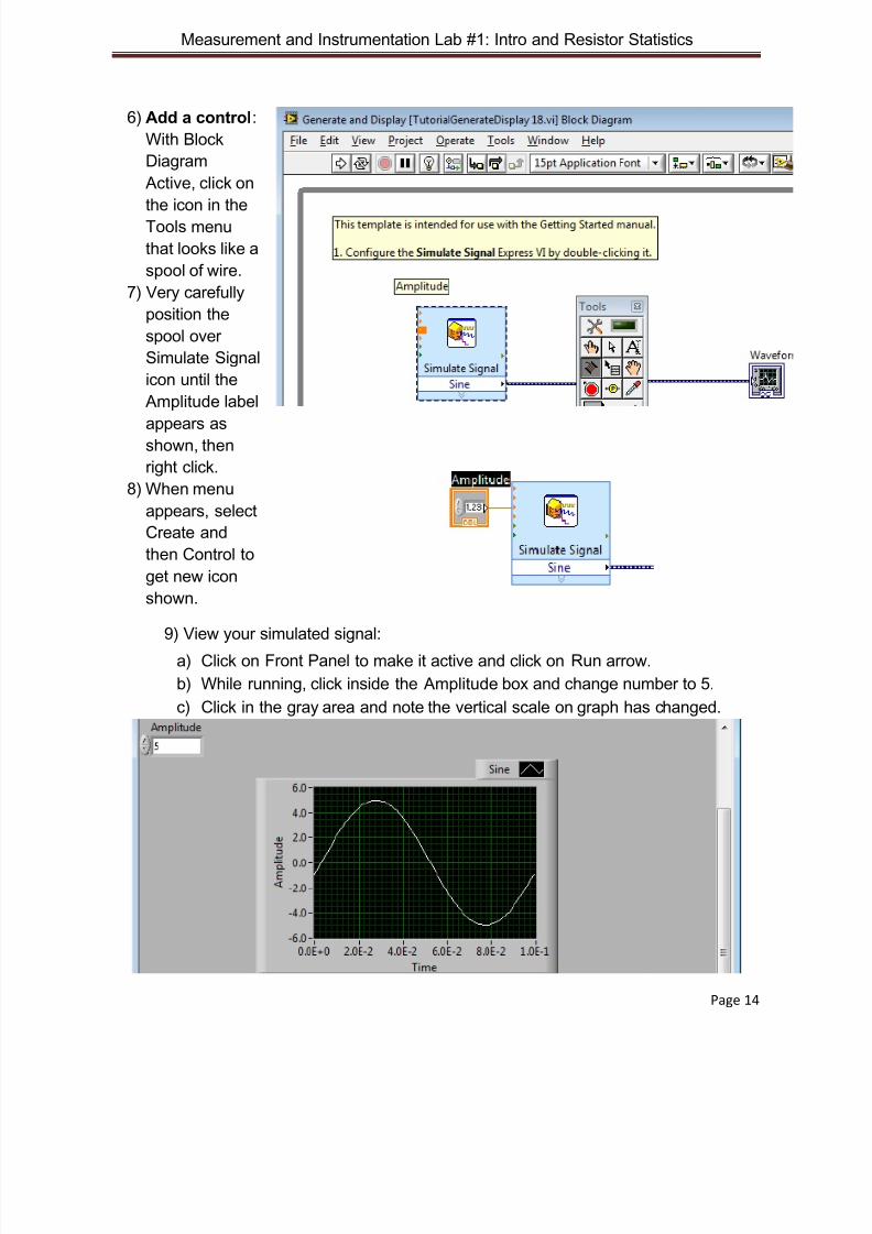
6) Add a control:
With Block
Diagram
Active, click on
the icon in theTools menu
that looks like a
spool of wire.
7) Very carefully
position the
spool over
Simulate Signal
icon until the
Amplitude label
appears asshown, then
right click.
8) When menu
appears, select
Create and
then Control to
get new icon
shown.
9) View your simulated signal:
a) Click on Front Panel to make it active and click on Run arrow.
b) While running, click inside the Amplitude box and change number to 5.
c) Click in the gray area and note the vertical scale on graph has changed.
8/13/2019 Lab Textbook (Partial)
http://slidepdf.com/reader/full/lab-textbook-partial 15/68
Measurement and Instrumentation Lab #1: Intro and Resistor Statistics
Page 15
Lab #1: Resistor Statistics
The most important part of taking good data in an experiment is planning what youwill be doing and how you will do it. If you go into an experiment thinking that you willtake all the data first and then figure out what you did later, there is a statistically highprobability that you will not take complete data and have to redo part of it => Effectiveplanning and understanding what you do FIRST saves time later.
This lab has 4 parts, to be done in this order:
1) LabVIEW Tutorial and statement in your notebook.2) Prepare your lab notebook, including all of Section II:
i. Overview (General foundations => specific methods)ii. Philosophy of Designiii. Design your experimental setup and procedureiv. Notes on needs for good data
3) Take lab data, including sketch in notebook and 2 data files4) Analyze data in LabVIEW and complete Uncertainty Analysis
Photos below show typical equipment and parts that you will be using. The actualequipment and parts at your work station may be a little bit different, but similar to whatis shown here.
Note that each individual person will have a different set of 10 resistors tomeasure, but each group of resistors will be used later by multiple people. So please becareful and try to keep resistors stuck the masking tape as you received them.
In Section II of lab (prelab) notebook, be sure to write down what you expect to find
for results, but do not be surprised if that result is different than what was expected, andbe ready to explain the potential reasons for the difference.
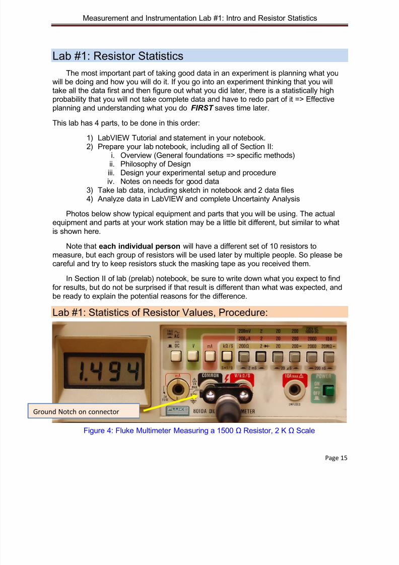
Lab #1: Statistics of Resistor Values, Procedure:
Figure 4: Fluke Multimeter Measuring a 1500 Ω Resistor, 2 K Ω Scale
Ground Notch on connector

8/13/2019 Lab Textbook (Partial)
http://slidepdf.com/reader/full/lab-textbook-partial 16/68
Measurement and Instrumentation Lab #1: Intro and Resistor Statistics
Page 16
Figure 5: Clips Attached to Resistor
Number Color 2 digits for 4-
band code
3 digits for 5
band code
Multiplier
# of 0’s after digits
Tolerance
0 Black
1 Brown ± 1%
2 Red ± 2 %
3 Orange4 Yellow
5 Green ± 0.5 %
6 Blue ± 0.25
7 Violet ± 0.1 %
8 Grey ± 0.05 %
9 White
Gold ± 5%
Silver ± 10%
Figure 6: Color code for Resistors
Carbon composition resistor, 270 K, 5% Film resistor, 270K, 5%
Figure 7: Types of Resistors
If resistor uses 4 bands for value, then tolerance can be 2, 5, or 10%
If resistor uses 5 bands for value, then tolerance can be 0.05, 0.1, 0.25, 0.5, or 1 %
Notes on collecting resistor data:
1) Record brand, model, serial #, tolerance spec. of your Ohm-meter
2) Each person (not group) will measure 10 resistors and record values in aWindows Notepad file, separated by commas. Give it file extension “.LVM”[set windows to show file extensions. Windows Explorer=>Organize=> Folderand search…=>View=> un-tick Hide File Extensions]
3) Do NOT remove resistors from tape that holds them together.
8/13/2019 Lab Textbook (Partial)
http://slidepdf.com/reader/full/lab-textbook-partial 17/68
Measurement and Instrumentation Lab #1: Intro and Resistor Statistics
Page 17
4) Each person in each group will individually take 10 measurements. Thencombine data for a group of at least 4 => the second data file will have 40 ormore values.
5) Resistor value may be labeled 1,500 ohms and 5% tolerance. Standard
tolerances are 1%, 5%, 10 %, so the values you read could more than 1% offand less than 10% over full temperature range, but may be more accuratethan this. Remember that meter has a tolerance also.
6) Plug dual banana plug into meter as shown. Side with plastic notch goes onthe negative/ground/common/black hole. Alternatively, the side with red markon it goes in the positive/red/ hole, also labeled V/kΩ/S.
7) Verify that two buttons are depressed: KΩ/S and 2 (2K [thousand] ohms fullscale=> maximum reading 1.999).
8) Each person must measure and record (in lab notebook) the values of eachof the 10 resistors on the string given. Different string for each person.
9) Within Windows, open All Programs=> Accessories=>Notepad
10) Type in values measured and save file as: 293_<your lastname>_10resistors.txt Separate data by commas. No return key !
11) After each person in your group has recorded 10 resistors, then one personshould combine all of the values so that you have a total of 40 or 50 values.Save the combined file as: 293_<your group name>_CombinedResistors.txt[Edit both files in Windows File Manager to change file extension from .txt to.lvm [.LVM] so that LabVIEW can read them properly.]
Use LabView for Analysis; Build File, Display Virtual Instrument (VI):
1) Start LabVIEW [Start => National Instruments => LabVIEW]
2) Open a new Blank VI [Virtual Instrument ]
3) Click in the Block Diagram window to make it active
4) View menu => Functions Palette => Click double arrow at bottom of window toexpand it => click on Express group=> click on Input group within Express
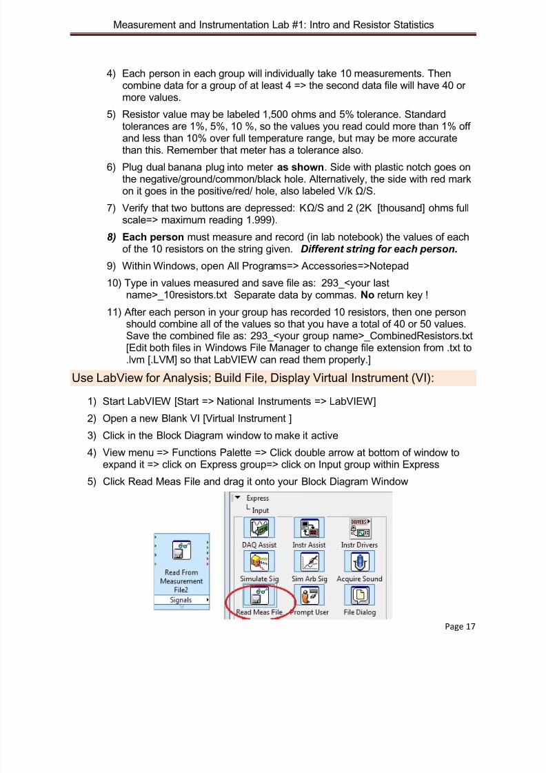
5) Click Read Meas File and drag it onto your Block Diagram Window
8/13/2019 Lab Textbook (Partial)
http://slidepdf.com/reader/full/lab-textbook-partial 18/68
Measurement and Instrumentation Lab #1: Intro and Resistor Statistics
Page 18
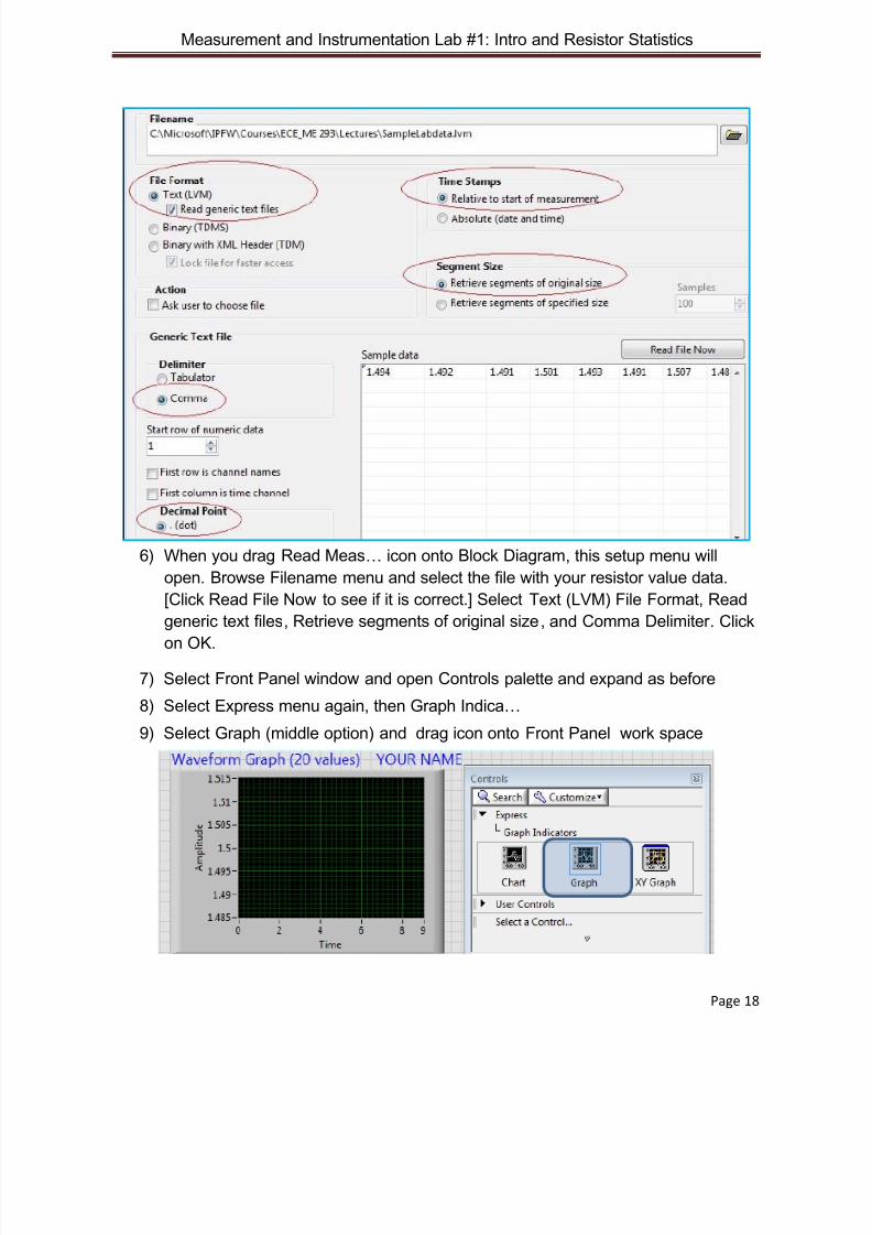
6) When you drag Read Meas… icon onto Block Diagram, this setup menu will
open. Browse Filename menu and select the file with your resistor value data.
[Click Read File Now to see if it is correct.] Select Text (LVM) File Format, Read
generic text files, Retrieve segments of original size, and Comma Delimiter . Click
on OK.
7) Select Front Panel window and open Controls palette and expand as before
8) Select Express menu again, then Graph Indica…
9) Select Graph (middle option) and drag icon onto Front Panel work space
8/13/2019 Lab Textbook (Partial)
http://slidepdf.com/reader/full/lab-textbook-partial 19/68
Measurement and Instrumentation Lab #1: Intro and Resistor Statistics
Page 19
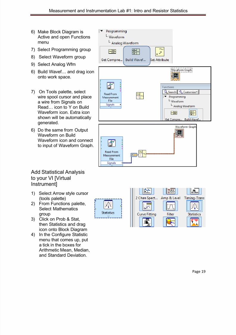
6) Make Block Diagram isActive and open Functions menu
7) Select Programming group
8) Select Waveform group
9) Select Analog Wfm
6) Build Wavef… and drag icononto work space.
7) On Tools palette, selectwire spool cursor and placea wire from Signals onRead… icon to Y on Build
Waveform icon. Extra iconshown will be automaticallygenerated.
6) Do the same from OutputWaveform on BuildWaveform icon and connectto input of Waveform Graph.
Add Statistical Analysisto your VI [VirtualInstrument]
1) Select Arrow style cursor(tools palette)
2) From Functions palette,Select Mathematicsgroup
3) Click on Prob & Stat,then Statistics and drag
icon onto Block Diagram4) In the Configure Statistic
menu that comes up, puta tick in the boxes for
Arithmetic Mean, Median,and Standard Deviation.
8/13/2019 Lab Textbook (Partial)
http://slidepdf.com/reader/full/lab-textbook-partial 20/68
Measurement and Instrumentation Lab #1: Intro and Resistor Statistics
Page 20
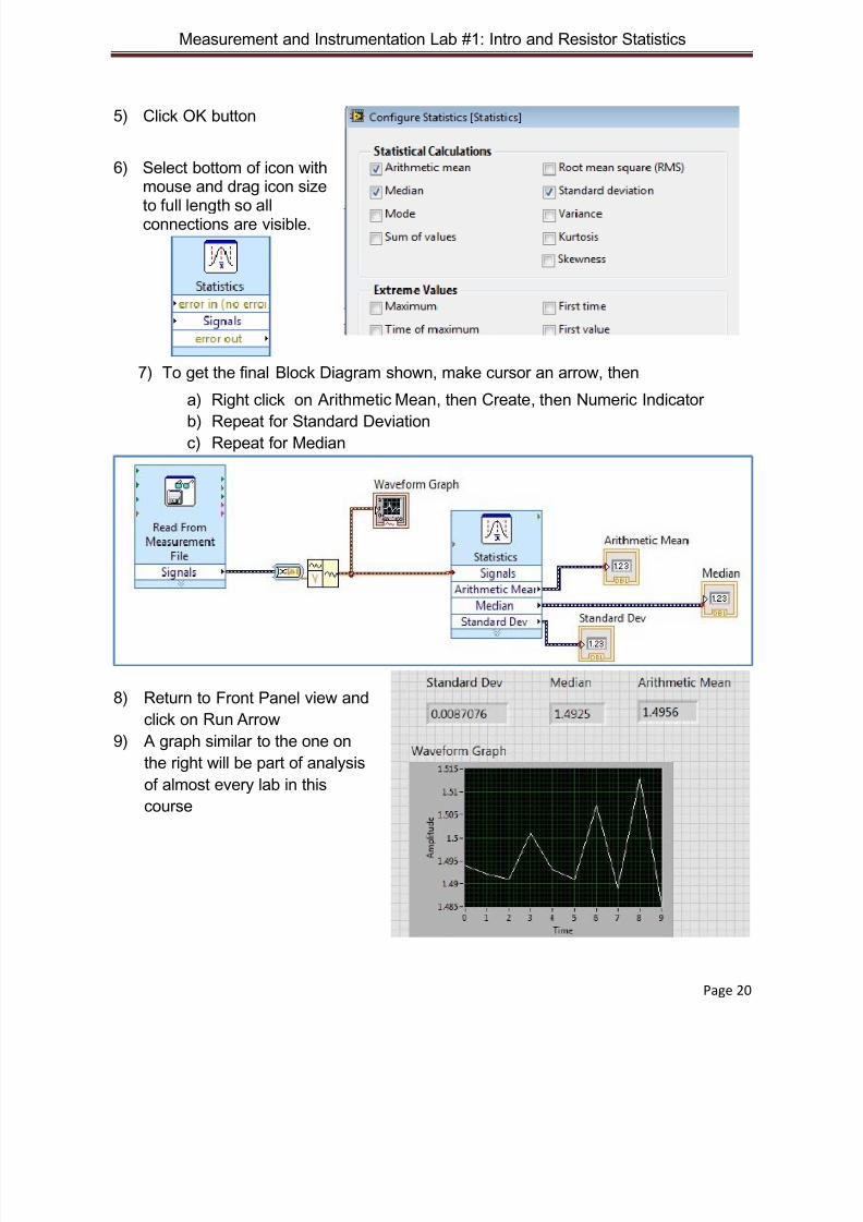
5) Click OK button
6) Select bottom of icon withmouse and drag icon size
to full length so allconnections are visible.
7) To get the final Block Diagram shown, make cursor an arrow, then
a) Right click on Arithmetic Mean, then Create, then Numeric Indicator
b) Repeat for Standard Deviation c) Repeat for Median
8) Return to Front Panel view and
click on Run Arrow
9) A graph similar to the one on
the right will be part of analysis
of almost every lab in this
course
8/13/2019 Lab Textbook (Partial)
http://slidepdf.com/reader/full/lab-textbook-partial 21/68
Measurement and Instrumentation Lab #1: Intro and Resistor Statistics
Page 21
Notes on Procedure for this lab:
1) Do the Labview Tutorial. When you have completed creating all screensshown in the above notes, write a statement in your notebook to that effect.Then print out your final sine wave display and attach it also to your notebook.
2) Create Section II, Design…:[Introduction]3) Each person needs to fill in all standard sections of lab
4) Each person needs to individually measure and record values for 10 resistors,
then create a notepad file with these values.
5) In a new Notepad file, add resistor values for at least 3 other people (40
values or more) and re-plot statistics in LabView. Lab notebook needs to
include a block diagram printout and two charts of R value Statistics, one for
10 values and one for 40 or more values.
6) Be sure to do error analysis and Uncertainty Budget (see separate document
for instructions on Uncertainty Budget.)
Lab Notebook:
All sections must be included, even if “empty,” or you will receive zero points for that
section.
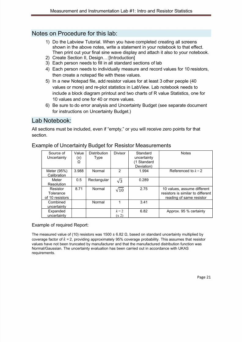
Example of Uncertainty Budget for Resistor Measurements
Source ofUncertainty
Value(±)Ω
DistributionType
Divisor Standarduncertainty(1 StandardDeviation)
Notes
Meter (95%)
Calibration
3.988 Normal 2 1.994 Referenced to k = 2
MeterResolution
0.5 Rectangular √ 3 0.289
ResistorTolerance
of 10 resistors
8.71 Normal √ 10 2.75 10 values, assume differentresistors is similar to different
reading of same resistorCombineduncertainty
Normal 1 3.41
Expandeduncertainty
k = 2
(x 2)6.82 Approx. 95 % certainty
Example of required Report:
The measured value of (10) resistors was 1500 ± 6.82 Ω, based on standard uncertainty multiplied by
coverage factor of k = 2, providing approximately 95% coverage probability. This assumes that resistorvalues have not been truncated by manufacturer and that the manufactured distribution function wasNormal/Gaussian. The uncertainty evaluation has been carried out in accordance with UKASrequirements.
8/13/2019 Lab Textbook (Partial)
http://slidepdf.com/reader/full/lab-textbook-partial 22/68
8/13/2019 Lab Textbook (Partial)
http://slidepdf.com/reader/full/lab-textbook-partial 23/68
Measurement and Instrumentation Lab #2: System Loading
Page 23
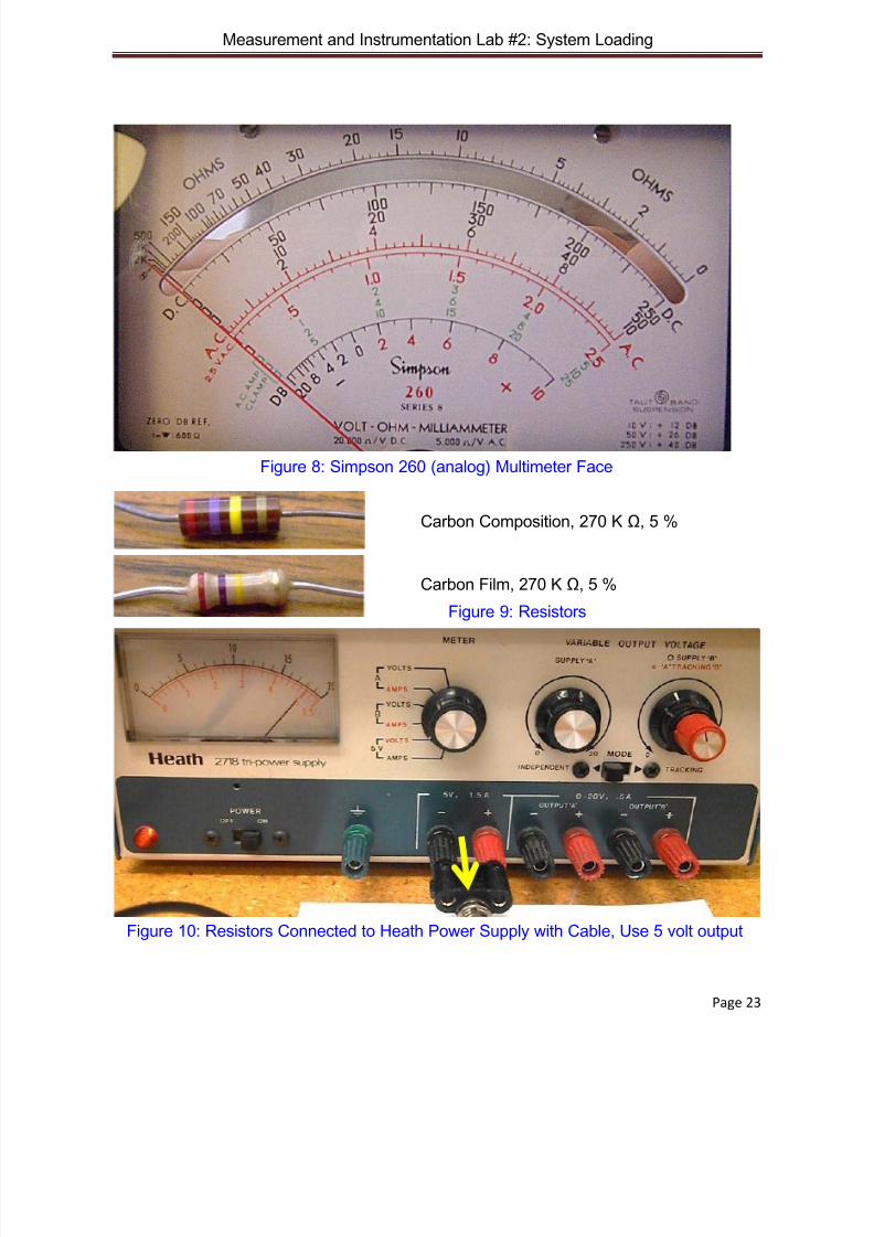
Figure 8: Simpson 260 (analog) Multimeter Face
Carbon Composition, 270 K Ω, 5 %
Carbon Film, 270 K Ω, 5 %
Figure 9: Resistors
Figure 10: Resistors Connected to Heath Power Supply with Cable, Use 5 volt output

8/13/2019 Lab Textbook (Partial)
http://slidepdf.com/reader/full/lab-textbook-partial 24/68
Measurement and Instrumentation Lab #2: System Loading
Page 24
Figure 11: Resistors Connected to HP Power Supply with Cable, note position of notch
Figure 12: Connect Resistors
Figure13: Fluke 45 Digital Multimeter
Notch on common bottom
Press up and down
buttons to select
display scale as shown
Hold (reading) button
Power Button
Set to 6 volt output to 5 volts and measure with Digital meter
1. Connect one side of eachresistor to one clip frompower supply cable
2. Connect black clip frommeter to black clip frompower supply
3. Use red clip from meter tohold resistors together
(cross leads).
8/13/2019 Lab Textbook (Partial)
http://slidepdf.com/reader/full/lab-textbook-partial 25/68

8/13/2019 Lab Textbook (Partial)
http://slidepdf.com/reader/full/lab-textbook-partial 26/68
Measurement and Instrumentation Lab #2: System Loading
Page 26
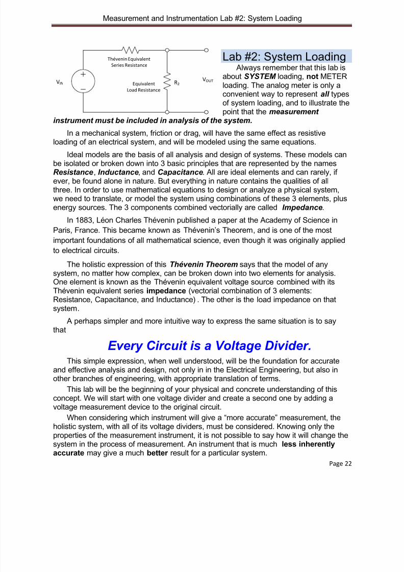
VIN R2
Thévenin Equivalent
Series Resistance
EquivalentLoad Resistance
VOUT
Figure 15: Voltage Source Equivalent Circuit with Load
This applies generally to all types of sources and loads, but for simplicity we will startwith simple ideal resistances. [Resistance, Inductance, Capacitance addedvectorially make impedance]
Method:
1) Separate the component to be analyzed from the rest of the circuit2) Consolidate the entire remaining circuit into a single source and seriesresistance
VIN
R1
R2
Thévenin Equivalent
Series Resistance
Equivalent
Load Resistance
VOUT
Figure 16: Thévenin Equivalent Voltage Divider
Example of Voltage Divider method for the above figure (not your lab):
The value used for R2 MUST include internal impedance of the measurement
instrument or there can be large error !
Some examples of typical internal resistances:
1) Ideal power supply has zero series resistance.
2) A typical regulated power supply has close to zero resistance within itsspecified operating range
21
2
R R
RV V IN OUT +
= ( )
V K K
K V
R R
RV V IN R 10
390390
39020
21
22 =
Ω+ΩΩ
=+
=

8/13/2019 Lab Textbook (Partial)
http://slidepdf.com/reader/full/lab-textbook-partial 27/68
Measurement and Instrumentation Lab #2: System Loading
Page 27
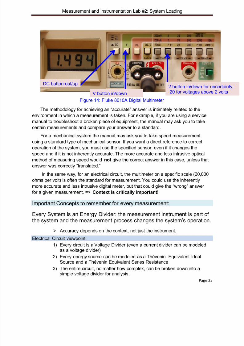
3) A Digital Multimeter typically has about 10 million ohms effective loadingresistance on a circuit
4) An Analog Multimeter is much more similar to adding another part, such as anamplifier, to a circuit.
5) The traditional standard for an analog voltmeter is 20,000 ohms per volt. Thatmeans that, if you set the meter to the 10 volts full scale, making ameasurement adds 10 x 20k = 200k Ω in parallel with your circuit.
Generally:
If a meter (or other circuit element) has internal resistance much greaterthan system, it will not “load” the system or substantially change its nature. Ifmeter resistance is similar to, or smaller than, the component beingmeasured, the system can change substantially. For example, you may add a“standard” amplifier with a gain of 100 to your circuit, expecting voltage to beamplified by 100. If impedances have not been accounted for, the “real” gain
may only be only 50.
How to Measure DC Voltage:
1) Set small knob on left to + DC
2) Set large scale switch to 10 V
3) Insert black wire into Common hole
4) Insert Red wire into + hole
5) Note that 10 volt scalemultiplied by 20,000 Ω/voltgives an internal meterresistance of 200 kΩ. Insidethe multimeter, there is literallya resistor of about 200kΩplaced in series with a lowimpedance current meter.
Figure 17: Simpson 260 Series Analog Multimeter
How to calculate the value of series and parallel resistors
8/13/2019 Lab Textbook (Partial)
http://slidepdf.com/reader/full/lab-textbook-partial 28/68
Measurement and Instrumentation Lab #2: System Loading
Page 28
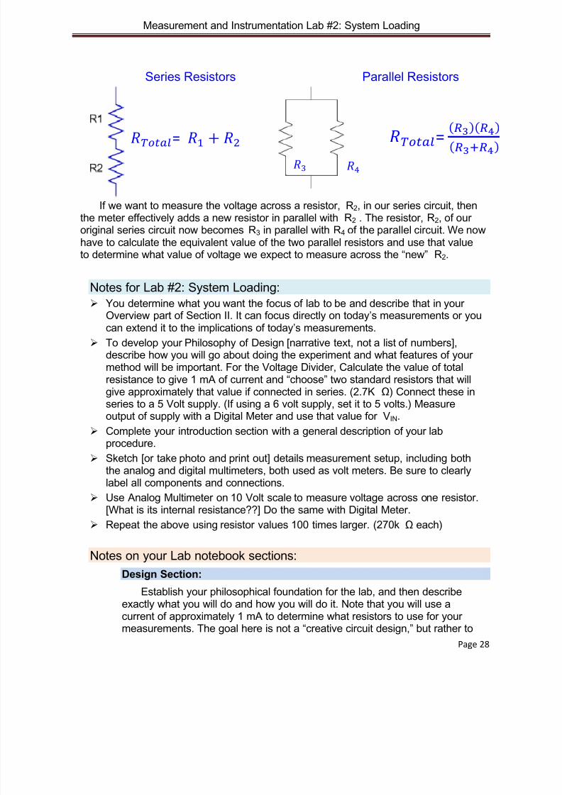
Series Resistors Parallel Resistors
If we want to measure the voltage across a resistor, R2, in our series circuit, thenthe meter effectively adds a new resistor in parallel with R2 . The resistor, R2, of ouroriginal series circuit now becomes R3 in parallel with R4 of the parallel circuit. We nowhave to calculate the equivalent value of the two parallel resistors and use that valueto determine what value of voltage we expect to measure across the “new” R2.
Notes for Lab #2: System Loading: You determine what you want the focus of lab to be and describe that in your
Overview part of Section II. It can focus directly on today’s measurements or youcan extend it to the implications of today’s measurements.
To develop your Philosophy of Design [narrative text, not a list of numbers],describe how you will go about doing the experiment and what features of yourmethod will be important. For the Voltage Divider, Calculate the value of totalresistance to give 1 mA of current and “choose” two standard resistors that willgive approximately that value if connected in series. (2.7K Ω) Connect these in
series to a 5 Volt supply. (If using a 6 volt supply, set it to 5 volts.) Measureoutput of supply with a Digital Meter and use that value for VIN.
Complete your introduction section with a general description of your labprocedure.
Sketch [or take photo and print out] details measurement setup, including boththe analog and digital multimeters, both used as volt meters. Be sure to clearlylabel all components and connections.
Use Analog Multimeter on 10 Volt scale to measure voltage across one resistor.[What is its internal resistance??] Do the same with Digital Meter.
Repeat the above using resistor values 100 times larger. (270k Ω each)
Notes on your Lab notebook sections:
Design Section:
Establish your philosophical foundation for the lab, and then describeexactly what you will do and how you will do it. Note that you will use acurrent of approximately 1 mA to determine what resistors to use for yourmeasurements. The goal here is not a “creative circuit design,” but rather to
=(
)(
)
(+) = 1 + 2
3 4

8/13/2019 Lab Textbook (Partial)
http://slidepdf.com/reader/full/lab-textbook-partial 29/68
Measurement and Instrumentation Lab #2: System Loading
Page 29
understand how that design would be implemented. You need to explain howyou came up with the circuit element values that have already been chosenand given to you, but do NOT say that in your notebook. Write the notebookas if you are designing the circuit.
What you are actually assigned to do is to Design the Experiment, or themethod of experiencing the measurement, not the details of circuit design,which you will do in a later course. The emphasis of this course is toexperience the nature of a circuit and measurement of the system properties,including a circuit. Part of that includes understanding the basics of how youcould have arrived at specific circuit values for your experiment.
Procedure Section:
1) Draw every circuit diagram associated with your design section andlabel all components.
2) List equations with descriptions of what they are for, substitute inlabels and numbers consistent with design section and with circuitdiagram (schematic).
3) List values for each component next to circuit diagram.4) Be sure to calculate the expected voltages that you will measure.5) Create a clearly labeled table with spaces for all of your data. Be
sure to label which meter is taking data (part of table). AFTERcreating the circuit diagram and data table, then take data andrecord it in your table. Table should have a space for calculateddata and for measured data of each type. Also leave space foruncertainty and percentage error.
6) Be sure to include statistical analysis graph from LabVIEW,uncertainty analysis, and discussion of all analysis and results.
[simplified] Uncertainty Analysis
Do statistical analysis of your 4 measurements in LabVIEW and print a chart similar tothis one:
8/13/2019 Lab Textbook (Partial)
http://slidepdf.com/reader/full/lab-textbook-partial 30/68
Measurement and Instrumentation Lab #2: System Loading
Page 30
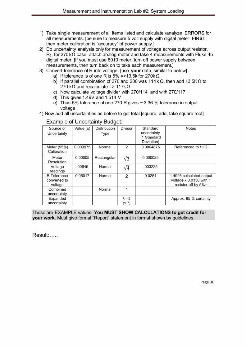
1) Take single measurement of all items listed and calculate /analyze ERRORS forall measurements. [be sure to measure 5 volt supply with digital meter FIRST,then meter calibration is “accuracy” of power supply.]
2) Do uncertainty analysis only for measurement of voltage across output resistor,R2, for 270 kΩ case, attach analog meter and take 4 measurements with Fluke 45
digital meter. [If you must use 8010 meter, turn off power supply betweenmeasurements, then turn back on to take each measurement.]
3) Convert tolerance of R into voltage: [use your data, similar to below]a) If tolerance is of one R is 5% =>13.5k for 270kΩ b) If parallel combination of 270 and 200 was 114kΩ, then add 13.5KΩ to
270 kΩ and recalculate => 117kΩ c) Now calculate voltage divider with 270/114 and with 270/117d) This gives 1.49V and 1.514 Ve) Thus 5% tolerance of one 270 R gives ~ 3.36 % tolerance in output
voltage4) Now add all uncertainties as before to get total [square, add, take square root]
Example of Uncertainty Budget:Source of
Uncertainty
Value (±) Distribution
Type
Divisor Standarduncertainty(1 StandardDeviation)
Notes
Meter (95%)Calibration
0.000975 Normal 2 0.0004875 Referenced to k = 2
MeterResolution
0.00005 Rectangular √ 3 0.000025
Voltagereadings
.00645 Normal √ 4 .003225
R Toleranceconverted tovoltage
0.05017 Normal 2 0.0251 1.4926 calculated outputvoltage x 0.0336 with 1resistor off by 5%=
Combineduncertainty
Normal 1
Expandeduncertainty
k = 2
(x 2)Approx. 95 % certainty
These are EXAMPLE values. You MUST SHOW CALCULATIONS to get credit foryour work. Must give formal “Report” statement in format shown by guidelines.
Result:…..
8/13/2019 Lab Textbook (Partial)
http://slidepdf.com/reader/full/lab-textbook-partial 31/68
Measurement and Instrumentation Lab #3: Atomic Structure/ Calibration
Page 31
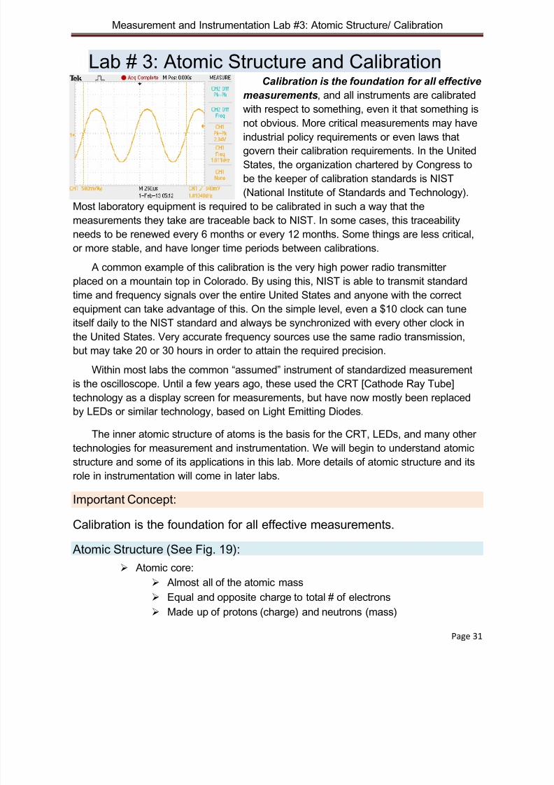
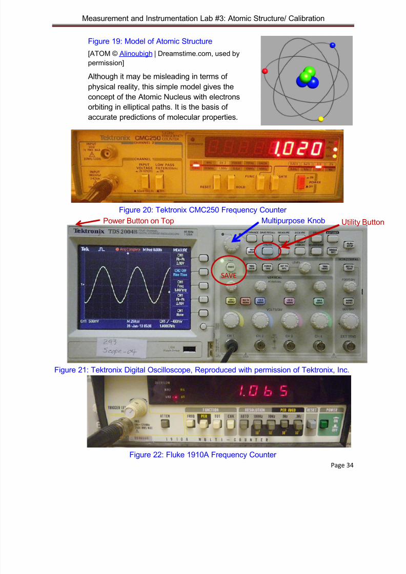
Lab # 3: Atomic Structure and CalibrationCalibration is the foundation for all effective
measurements, and all instruments are calibrated
with respect to something, even it that something is
not obvious. More critical measurements may have
industrial policy requirements or even laws thatgovern their calibration requirements. In the United
States, the organization chartered by Congress to
be the keeper of calibration standards is NIST
(National Institute of Standards and Technology).
Most laboratory equipment is required to be calibrated in such a way that the
measurements they take are traceable back to NIST. In some cases, this traceability
needs to be renewed every 6 months or every 12 months. Some things are less critical,
or more stable, and have longer time periods between calibrations.
A common example of this calibration is the very high power radio transmitterplaced on a mountain top in Colorado. By using this, NIST is able to transmit standard
time and frequency signals over the entire United States and anyone with the correct
equipment can take advantage of this. On the simple level, even a $10 clock can tune
itself daily to the NIST standard and always be synchronized with every other clock in
the United States. Very accurate frequency sources use the same radio transmission,
but may take 20 or 30 hours in order to attain the required precision.
Within most labs the common “assumed” instrument of standardized measurement
is the oscilloscope. Until a few years ago, these used the CRT [Cathode Ray Tube]
technology as a display screen for measurements, but have now mostly been replacedby LEDs or similar technology, based on Light Emitting Diodes.
The inner atomic structure of atoms is the basis for the CRT, LEDs, and many other
technologies for measurement and instrumentation. We will begin to understand atomic
structure and some of its applications in this lab. More details of atomic structure and its
role in instrumentation will come in later labs.
Important Concept:
Calibration is the foundation for all effective measurements.
Atomic Structure (See Fig. 19):
Atomic core:
Almost all of the atomic mass
Equal and opposite charge to total # of electrons
Made up of protons (charge) and neutrons (mass)

8/13/2019 Lab Textbook (Partial)
http://slidepdf.com/reader/full/lab-textbook-partial 32/68
Measurement and Instrumentation Lab #3: Atomic Structure/ Calibration
Page 32
Electrons effectively “rotate” around the nucleus and have a “stochastic”location and size
Each orbital has a distinctly defined energy level. Electrons virtually neverexist outside their defined (quantized) energy level.
Niels Bohr (Danish): 1922 Nobel Prize for understanding the structure of atoms:
Neils Bohr => Bohr Atom
1) Classical charge radiates energywhenever it accelerates
2) The electron has a wavelikenature
3) If the wave property of theelectron bound to an atom isself-coherent, then it can “liveforever” without radiating anyenergy
4) Bound electrons can only existat discrete energy levels
5) Electrons only change states bygaining or losing the energydifference between bands/levels
Properties of the Cathode Ray Tube Oscilloscope:
1) A beam of electrons is scanned horizontally across the front face of a glass tube.
During the scan, applied Voltage (signal to be measured) deflects the beamvertically. When electrons hit phosphor coating on the surface of the tube, otherelectrons are excited to a higher energy level within the atom. When the excitedelectrons decay back to their original energy level, they radiate light, which isobserved as an image on the surface of the tube.
2) For some 70 years, the CRT was our main method of visualizing electronicwaveforms and signals.
3) Electrons in the beam have been accelerated by a potential of 10,000 to 20,000volts
4) A similar structure is used for the electron microscope, our major method ofseeing the microscopic world. (Electrons accelerated from 30,000 to millions ofvolts)
5) Similar structure to TV tube (10 to 30 thousand volts)
6) Similar to modern microwave vacuum tubes
8/13/2019 Lab Textbook (Partial)
http://slidepdf.com/reader/full/lab-textbook-partial 33/68
Measurement and Instrumentation Lab #3: Atomic Structure/ Calibration
Page 33
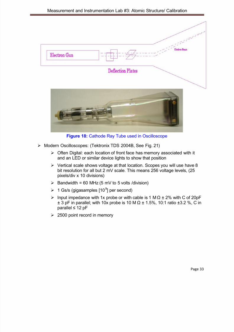
Figure 18: Cathode Ray Tube used in Oscilloscope
Modern Oscilloscopes: (Tektronix TDS 2004B, See Fig. 21)
Often Digital: each location of front face has memory associated with itand an LED or similar device lights to show that position
Vertical scale shows voltage at that location. Scopes you will use have 8
bit resolution for all but 2 mV scale. This means 256 voltage levels, (25pixels/div x 10 divisions)
Bandwidth = 60 MHz (5 mV to 5 volts /division)
1 Gs/s (gigasamples [109] per second)
Input impedance with 1x probe or with cable is 1 MΩ ± 2% with C of 20pF± 3 pF in parallel; with 10x probe is 10 MΩ ± 1.5%, 10:1 ratio ±3.2 %, C inparallel ≤ 12 pF
2500 point record in memory
8/13/2019 Lab Textbook (Partial)
http://slidepdf.com/reader/full/lab-textbook-partial 34/68
8/13/2019 Lab Textbook (Partial)
http://slidepdf.com/reader/full/lab-textbook-partial 35/68
Measurement and Instrumentation Lab #3: Atomic Structure/ Calibration
Page 35
Important Laboratory concepts:
Design of experiments, at the most basic level, is merely the organization of aproject. This organization should include careful planning so that the specific neededdata can be effectively and accurately obtained.
At a higher level, Design of Experiments represents the ultimate goal of allowinga manufacturing operation to achieve near ideal results on the “first implementation,”
a somewhat rare event. This would usually include a substantial statistical set ofmeasurements and analysis that would indicate the sensitivity of overall productperformance to each individual component. This sensitivity analysis allows thedesigner to put the highest quality parts where they will do the most good.
Universes (Domains) of Design and Measurement
For the universe we seem to live in, we virtually always experience ourselves aspart of the “Time Domain.” That means that everything is viewed as being a serialgroup of events that take place as time progresses, one after another.
The true universe that we live in, however, has many different levels andDomains. The Time Domain is only one of these. In order to effectively design a
complex system, the engineer has to understand how to take into account manydifferent domains. Only through this holistic understanding, can a laboratorymeasurement, a Design of Experiments, be completely effective and accurate.
In the Frequency Domain, a signal or activity is viewed and measured withrespect to its frequency components, rather than its progression in time. The Timeand Frequency domains can be translated back and forth, but each gives differentinformation about the signal and can have very different measurementcharacteristics. The success of modern communications systems is based veryheavily on the understanding of Frequency Domain characteristics of signals.
Within both of these domains, signals or events can be analyzed as eitherDeterministic or as Stochastic. In our normal activity, we experience things as
Deterministic => they have a specific and more or less constant value. For example,if you have 5 pennies in your pocket now, something specific has to happen in orderfor that number to change; you know its value. A Stochastic Process, however, hasno fixed value, only probabilities of what has or will happen. It would normally benecessary to take hundreds, or thousands of “trials” in order to produce an accurateStatistical model for a Stochastic process.
In nature, everything has both Deterministic and Stochastic properties thatcoexist at the same time. Quantum Mechanics, some hundred years ago, came upwith mathematical equations to represent both Deterministic (particle like) andStochastic (wavelike) properties. Today, however, humans still cannot conceptuallygrasp this process and cannot create experiments to measure both of theseproperties at the same time, so we have to combine different experiments to measurethe full nature of a process.
Within atoms, the result of Quantum Mechanics is that we have a model thatincludes both particle like nature as the size and mass of an electron, while at thesame time, quantized energy levels that reflect the wavelike nature of an electron andallow us to justify the “existence of the physical universe.” We could call thisdescription of the atom the Energy Level Domain, and by using it, we can make
8/13/2019 Lab Textbook (Partial)
http://slidepdf.com/reader/full/lab-textbook-partial 36/68
Measurement and Instrumentation Lab #3: Atomic Structure/ Calibration
Page 36
many types of precise measurements and effectively design essential products, likeoscilloscopes, semiconductors, LEDs, Lasers.
At an even deeper level of atomic structure, is what could be called theMomentum Domain, that can be used to describe other essential qualities of nature,such as negative resistance, a concept that defies explanation within the realm ofClassical Physics.
Lab Notes:
Think of yourself as an engineering professional being paid a high salary for yourservice and write your lab notebook from that viewpoint.
Do NOT
Refer to yourself as a student
Say or imply that you are “learning” => you are being paid as an expert, soreferences to things “learned” need to be stated as if significant, notsomething you do not know how to do
Complain about your assignment or your inability to understand. In theprofessional environment, this type of attitude could lead to you losingyour job.
You are given guidelines that are to be basis of your “Design of Experiment”and you are expected to design the lab so that you are able to get the dataneeded for the desired analysis.
Guidelines are flexible, but if you do nothing at all for a required section, or do notinclude needed sub sections, you will get no credit for that part. This is standardprofessional practice.
For Overview section, start with a general point, and then describe your Designof Experiments in terms of how you will demonstrate that point. State things as aprofessional proving a point, not as a student trying to “learn” something.
Procedural Guidelines for this lab: NEED USB Drive, 2 GB or smaller
1) First thing to do in lab is to turn on Oscilloscope and let it warm up. Press powerbutton on top of instrument, left side, and make sure lights come on. Startup willtake about one minute.
2) While waiting, turn on power for both Function Generator and Frequency Counter
3) Come back to scope and press button labeled, Utility.
4) The screen will change and show a menu along right side of screen. Pressbutton next to label, Do Self Calibration.
5) It will ask you to disconnect all cables from scope. Do this and then press buttonnext to OK.
6) There are 16 steps to self-calibration and it will take several minutes. While this isgoing on, first set up the Function Generator and then the Frequency Counter.After these have been calibrated, be very careful not to change any settings.Recheck calibration at end of the lab to verify accuracy. In a “real” situation, you

8/13/2019 Lab Textbook (Partial)
http://slidepdf.com/reader/full/lab-textbook-partial 37/68
Measurement and Instrumentation Lab #3: Atomic Structure/ Calibration
Page 37
may need 30 minutes or even several hours of warm-up time for equipmentstabilization.
Set up function Generator:
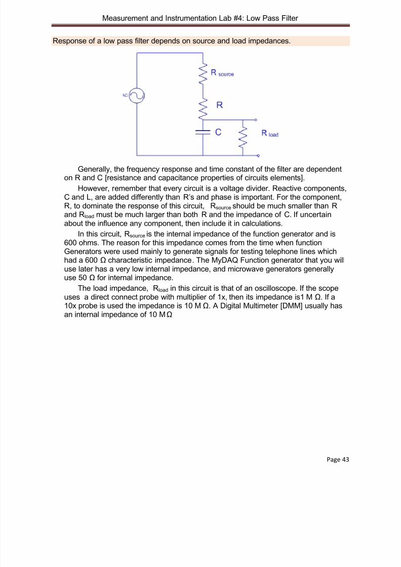
1) Turn on function Generator and allow to warm up, push LINE ON (IN) button attop left corner of front panel.
2) Press 1K button
3) Adjust large Knob to 1
4) Set amplitude similar to that shown and connect cable as shown, carefully noteposition of small black notch on connector (ground side).
Figure 23: Hewlett Packard 3311A Signal Generator
A Frequency counter will serve as our NIST (National Institute of Standards) reference.If using Tektronix Model CMC250, Fig. 20:
1) Turn on power and allow to warm up
2) Turn on Low Pass Filter and 3 V scale. Use Channel 1, lower connector.
3) Connect coaxial cable to Function generator
4) Press FUNC button until you get the reading shown, 4 digits.
5) Adjust Function Generator to get as close as possible to frequency displayshown (1.000 KHz). This will be your reference. Be careful not to changeFunction Generator while making other measurements.
6) Use uncertainty spec. = ± 1 digit of reading ( 1 Hz here) ± stability spec. of 0.1ppm of 10 MHz= 1 Hz
If using Fluke Model 1910A, Fig. 22:
1) Turn on power and allow meter to warm up.
2) Set function to FREQ (press button)
Power
Notch
8/13/2019 Lab Textbook (Partial)
http://slidepdf.com/reader/full/lab-textbook-partial 38/68
Measurement and Instrumentation Lab #3: Atomic Structure/ Calibration
Page 38
3) Set Resolution to 1 Hz (press button)
4) Connect coaxial cable to Function Generator
5) Adjust trigger level to get stable reading of frequency, may be slow/sensitive.
6) Adjust Function Generator to get as close as possible to display shown. This willbe your reference. Be careful not to change Function Generator.
7) Use uncertainty spec. = ± 1 digit of reading (1 Hz ) ± 0.1 ppm of 10 MHz= 1 Hz
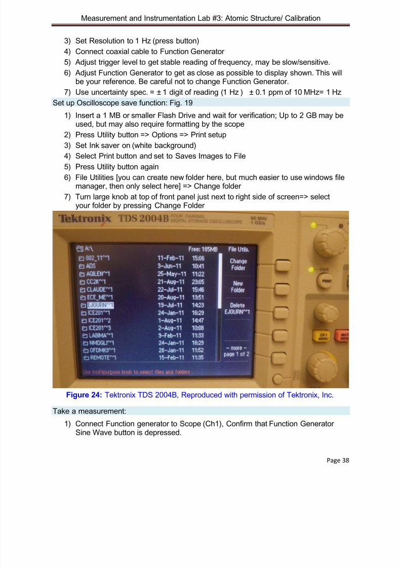
Set up Oscilloscope save function: Fig. 19
1) Insert a 1 MB or smaller Flash Drive and wait for verification; Up to 2 GB may beused, but may also require formatting by the scope
2) Press Utility button => Options => Print setup
3) Set Ink saver on (white background)
4) Select Print button and set to Saves Images to File
5) Press Utility button again
6) File Utilities [you can create new folder here, but much easier to use windows filemanager, then only select here] => Change folder
7) Turn large knob at top of front panel just next to right side of screen=> selectyour folder by pressing Change Folder
Figure 24: Tektronix TDS 2004B, Reproduced with permission of Tektronix, Inc.
Take a measurement:
1) Connect Function generator to Scope (Ch1), Confirm that Function GeneratorSine Wave button is depressed.
8/13/2019 Lab Textbook (Partial)
http://slidepdf.com/reader/full/lab-textbook-partial 39/68
Measurement and Instrumentation Lab #3: Atomic Structure/ Calibration
Page 39
2) Press CH 1 MENU on scope until waveform shows yellow (May need to turn offother channels)
3) Press Trigger Menu button and set source to CH1, set Slope to Rising, set Typeto Edge, set Mode to Normal
4) Adjust SEC/DIV knob to give M 250 µs at bottom of screen, as shown
5) Press PRINT button and clock will appear at bottom right side of screen until
screen has been saved6) Press Utility => File Utilities to see if file was recorded
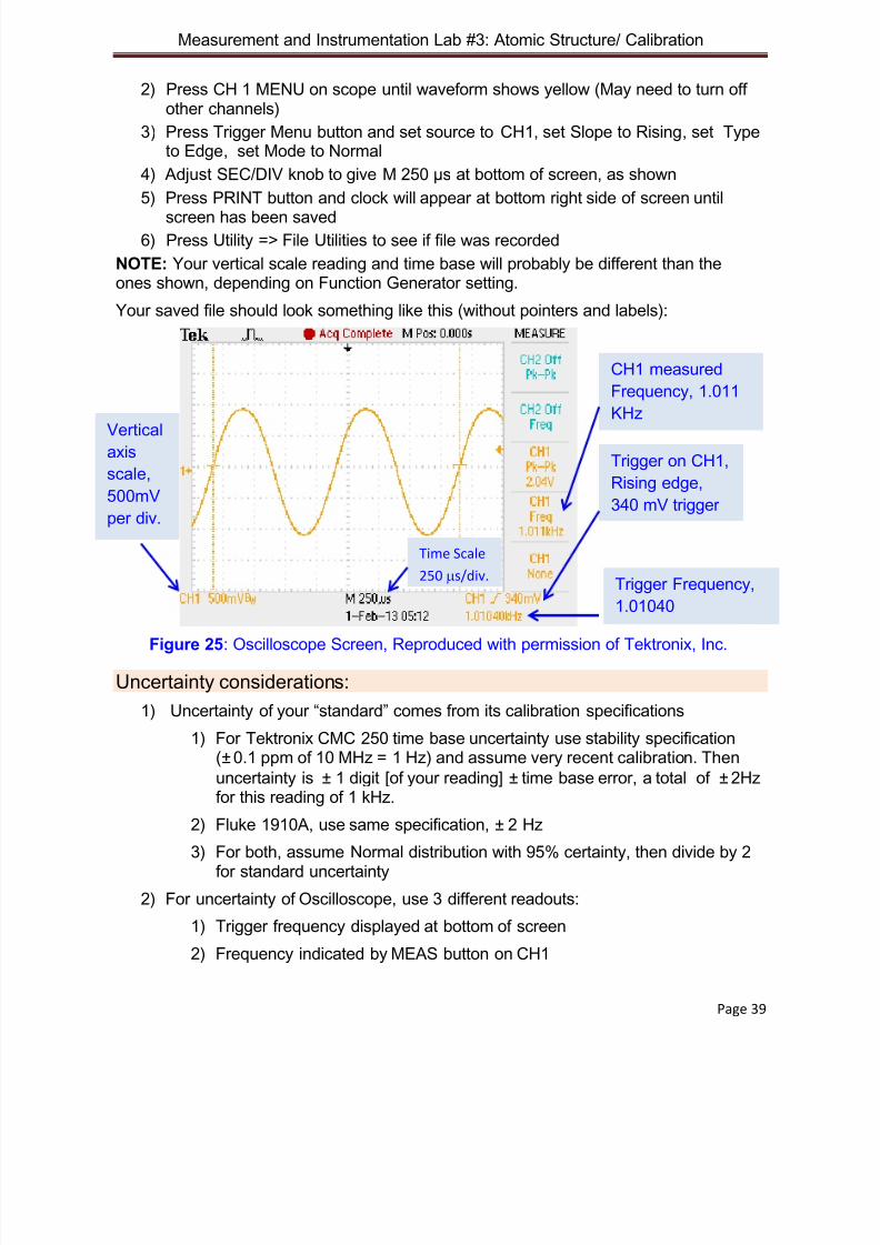
NOTE: Your vertical scale reading and time base will probably be different than theones shown, depending on Function Generator setting.
Your saved file should look something like this (without pointers and labels):
Figure 25: Oscilloscope Screen, Reproduced with permission of Tektronix, Inc.
Uncertainty considerations:
1) Uncertainty of your “standard” comes from its calibration specifications
1) For Tektronix CMC 250 time base uncertainty use stability specification(±0.1 ppm of 10 MHz = 1 Hz) and assume very recent calibration. Thenuncertainty is ± 1 digit [of your reading] ± time base error, a total of ±2Hzfor this reading of 1 kHz.
2) Fluke 1910A, use same specification, ± 2 Hz
3) For both, assume Normal distribution with 95% certainty, then divide by 2for standard uncertainty
2) For uncertainty of Oscilloscope, use 3 different readouts:
1) Trigger frequency displayed at bottom of screen
2) Frequency indicated by MEAS button on CH1
CH1 measured
Frequency, 1.011
KHz
Trigger on CH1,
Rising edge,
340 mV trigger
Trigger Frequency,
1.01040
Time Scale
250 µs/div.
Verticalaxis
scale,
500mV
per div.

8/13/2019 Lab Textbook (Partial)
http://slidepdf.com/reader/full/lab-textbook-partial 40/68
Measurement and Instrumentation Lab #3: Atomic Structure/ Calibration
Page 40
3) Frequency found by taking one over the period of screen display.[measure at least 2 cycles and use zero crossing position of waveform]
4) Treat these as 3 sequential readings and divide by √ 3 for standarduncertainty.
3) All uncertainty values must be in terms of Hz
Your uncertainty Budget should look similar to this. Add summary statement and show
calculations. Use LabVIEW VI from lab 1 to calculate data for measurements.
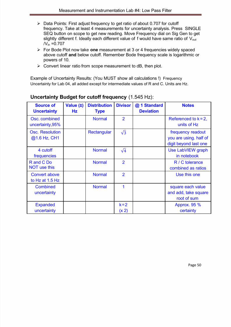
Uncertainty Budget [based on 1 KHz]:
Source of
Uncertainty
Value (±)
Hz
Distribution
Type
Divisor Standarduncertainty(1 S Dev)
Notes
F Counter(95%) Cal.
Normal 2 Referenced to k = 2
Counter
Resolution
Rectangular √ 3
Scope
indication of
measured
frequency=> 3
values
Normal √ 4 3 values, assume different
types are similar to
different readings of same
type
Combineduncertainty
Normal 1
Expanded
uncertainty
k = 2
(x 2)
Approx. 95 % certainty
Report:

8/13/2019 Lab Textbook (Partial)
http://slidepdf.com/reader/full/lab-textbook-partial 41/68
Measurement and Instrumentation Lab #4: Low Pass Filter
Page 41
Lab # 4: Low Pass Filter: Forced and Natural Responses
Discrimination is thebasis for effectiveoperation of virtually
every system in nature,whether it is an electricalcircuit, a mechanicalsystem, or computer logic.Within an electrical circuit,discrimination is described
by the term, Filter .
When we design the part of a circuit that discriminates, it is referred to as FilterDesign. Keep in mind, however, that every circuit has the filtering effect as part of itsnature, whether it is explicit or not.
There are many different categories and properties of Filters. One of the maindescriptions requires us to enter the Frequency Domain, and describe the Filter interms of how it discriminates with respect to Frequency. In this domain, there are 3fundamental types of Filters – a Low Pass Filter allows lower frequencies to proceedwith minimal reduction in amplitude; a High Pass Filter does the opposite, allowinghigher frequencies to proceed with little reduction in amplitude. Band Pass Filters,sometimes loosely called Resonant Filters, allow a range of frequencies to pass withminimal attenuation, while reducing the amplitude of both higher and lower frequencies.
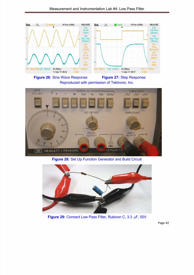
The same filters also have district characteristics in the Time Domain. One way todescribe the response of a filter in the time domain is to stimulate it with a Stepwaveform and then observe the Step Response. The Low Pass Filter has thecharacteristic of slowing down the rise and fall rates of a step waveform, as shown inFig. 27.
This experiment gives you the opportunity to understand the Concept of FrequencyDiscrimination through the design of a simple Low Pass Filter . In the process, you willduplicate the design, build the filter, and characterize its response.
Technically, the description of the Filter that you will use is called a First Order,Single Pole, Low Pass Filter and all filters of this type have the same shape ofFrequency Response, only with respect to different frequencies.
This experiment uses physical circuit elements to build a Low Pass Filter and a
physical (digital) oscilloscope to take measurements with manually set frequenciescoming from an analog signal generator.
Important concept:
Discrimination is the basis for effective operation of virtually every systemin nature.
8/13/2019 Lab Textbook (Partial)
http://slidepdf.com/reader/full/lab-textbook-partial 42/68
Measurement and Instrumentation Lab #4: Low Pass Filter
Page 42
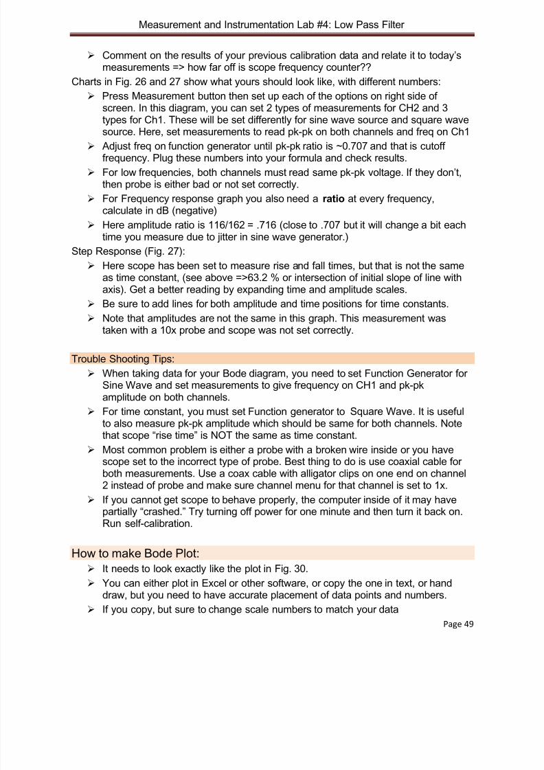
Figure 26: Sine Wave Response Figure 27: Step Response
Reproduced with permission of Tektronix, Inc.
Figure 28: Set Up Function Generator and Build Circuit
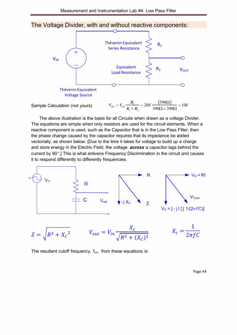
Figure 29: Connect Low Pass Filter, Rubicon C, 3.3 µF, 50V
8/13/2019 Lab Textbook (Partial)
http://slidepdf.com/reader/full/lab-textbook-partial 43/68
8/13/2019 Lab Textbook (Partial)
http://slidepdf.com/reader/full/lab-textbook-partial 44/68
Measurement and Instrumentation Lab #4: Low Pass Filter
Page 44
The Voltage Divider, with and without reactive components:
VIN
Thévenin Equivalent
Voltage Source
R1
R2
Thévenin Equivalent
Series Resistance
Equivalent
Load ResistanceVOUT
Sample Calculation (not yours)
The above illustration is the basis for all Circuits when drawn as a voltage Divider.The equations are simple when only resistors are used for the circuit elements. When a
reactive component is used, such as the Capacitor that is in the Low Pass Filter, then
the phase change caused by the capacitor requires that its impedance be added
vectorially, as shown below. [Due to the time it takes for voltage to build up a chargeand store energy in the Electric Field, the voltage across a capacitor lags behind the
current by 90°.] This is what enlivens Frequency Discrimination in the circuit and causes
it to respond differently to differently frequencies.
- j XC
R
ZVC = [ - j I ] [ 1/(2π f C)]
VR = RI
VTotal
= 2 + 2
The resultant cutoff frequency, f co, from these equations is:
( )V V
R R
RV V IN R 10
390390
39020
21
22 =
Ω+ΩΩ
=+
=
= 2 + ( )2 = 1
2
8/13/2019 Lab Textbook (Partial)
http://slidepdf.com/reader/full/lab-textbook-partial 45/68

8/13/2019 Lab Textbook (Partial)
http://slidepdf.com/reader/full/lab-textbook-partial 46/68
Measurement and Instrumentation Lab #4: Low Pass Filter
Page 46
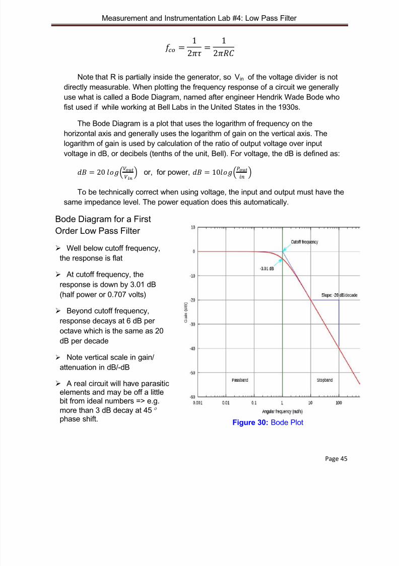
If frequency response is plotted with a linear vertical scale, then the right side of the
graph is not a straight line, but curves as shown below. Either way you need to use ratio
of Vout/Vin. For linear plot 0 to 1 and for dB the scale is negative.
= 2010 Log uses base 10 and number is negative because Vout
is smaller than Vin
When the total impedance of the circuit is dominantly R, real, there is no phase
difference between input and output voltages (f << f CO) When the total impedance of the circuit is dominantly C, reactive or imaginary, there
is 90° phase shift for each independent reactive component or pole in the circuit (f
>> f CO). Here we have one component so phase shift is a maximum of 90 °.
The cutoff frequency of a single pole circuit is defined as the point at which
magnitude has dropped by 3 dB. This MUST correspond to a phase shift of 45°.

8/13/2019 Lab Textbook (Partial)
http://slidepdf.com/reader/full/lab-textbook-partial 47/68
Measurement and Instrumentation Lab #4: Low Pass Filter
Page 47
It is not possible for voltage to change as a function of frequency unless there are
reactive/imaginary components in the model.
For the single pole Low Pass filter, ignoring
“extra” resistors, the cutoff frequency is given by:
At cutoff frequency the resistance of R is exactly the same as the “resistance” of
C. Thus, the phase shift is 45° . If we choose R to be 33,000Ω, then C comes out to be 2.4 µF for cutoff
frequency of 2 Hz. (Your lab will use 1.6 Hz) To justify ignoring other resistors, look at their comparative values at cutoff
frequency. Rsource is 600 Ω, much less than 33KΩ. Rload is 1 MΩ and muchgreater than 33 K of C.
If we excite the circuit with a square wave, then we get a different set of information,
the time constant of the Filter. (=RC)
For this example, the time constant is 33K x 2.4 x 10-6 = 0.0792 S.
Figure 31: Rise and Fall time constants
If the circuit is excited with a square wave of suitable period, then the leading edge
will show charging time constant and falling edge will show the discharge time
constant.
NOTE:
One time constant is at a position where voltage is 63.2 % of maximum for
rising edge. You need to use this in lab. If pk-pk voltage is different on CH1 and
CH2 with a square wave, either your probe is bad or scope is set incorrectly.
Illustration of how to wire your circuit: See Fig. 28 and 29.
Connect a cable to function generator. If using alligator clips instead of cable,connect Red one to “Hi” terminal as shown.
Connect negative side of Capacitor to Lo side of Function Generator output(Black alligator clip) and also to ground of oscilloscope channels. (connector side
=1
2 =1
2

8/13/2019 Lab Textbook (Partial)
http://slidepdf.com/reader/full/lab-textbook-partial 48/68
Measurement and Instrumentation Lab #4: Low Pass Filter
Page 48
with notch)
Do NOT twist wires together – cross one wire of C and one of R in an “X”pattern as shown and hold in place with Red alligator clip going to RC Filteroutput channel of scope, Ch2.
Input (of RC filter) channel of scope, CH1, and Hi side of function generatorconnect Red wires to the remaining wire of R, as shown.
Note that tab on coaxial banana plug is on “common” side that also servesas ground reference.
Lab Guidelines:
You will have available 30kΩ resistors and 3.3µF Capacitors
Design an experiment to validate material of the above notes.
As part of Experimental Design, verify the circuit design. Do this by starting withthe given 30kΩ resistor and the desired frequency for cutoff (1.6 Hz). Calculatethe capacitor needed. Then choose to use a standard value of capacitor, 3.3 µF.Using the new value for capacitor, recalculate expected cutoff frequency.
Support theoretically and by measurements that you are justified in being able toleave the source and load R’s out of your calculations.
Since you have different values than used in notes above, you need to redo allcalculations.
Take measurements to validate both Frequency Domain and Time Domain typesof response. You will need to choose several decades of frequencies for thelow pass filter and you will need to use a long enough period (low enoughfrequency setting on Function Generator) of square wave to see rise and falltimes. Calculate desired frequency for square wave before doing measurement.(To see full response, let half period of square wave be larger than rise time of
filter => use 6 times rise time and set Function Generator Frequency to one overthis, period is one over frequency => Explain this in introduction.)
Plot/sketch frequency response on a Bode Diagram [ratio of output to input in dBon vertical axis, log frequency on horizontal axis]=> set generator to sine wave.Take measurements across output of function generator on CH1, across C onCH2 of scope. Make sure BOTH black wires are connected toground/common terminal.
Scope has to be set to trigger in “normal” mode for MEASURE to work. IF youset everything as described and waveform does not update as expected, thenpress the button, Force Trig.
Print the screen shot for rise and fall as a time based graph=> set generator tosquare wave. Make it LARGE ! Sketch lines on graph for time constant.
For both plots, print out oscilloscope screen and attach to your notebook. For
Frequency Domain, you only need to print screen shot of one frequency and then
make a table for other frequencies. Time domain needs to be large enough to
clearly show data and hand-marked for measurement points.
8/13/2019 Lab Textbook (Partial)
http://slidepdf.com/reader/full/lab-textbook-partial 49/68
Measurement and Instrumentation Lab #4: Low Pass Filter
Page 49
Comment on the results of your previous calibration data and relate it to today’smeasurements => how far off is scope frequency counter??
Charts in Fig. 26 and 27 show what yours should look like, with different numbers:
Press Measurement button then set up each of the options on right side ofscreen. In this diagram, you can set 2 types of measurements for CH2 and 3types for Ch1. These will be set differently for sine wave source and square wave
source. Here, set measurements to read pk-pk on both channels and freq on Ch1 Adjust freq on function generator until pk-pk ratio is ~0.707 and that is cutoff
frequency. Plug these numbers into your formula and check results.
For low frequencies, both channels must read same pk-pk voltage. If they don’t,then probe is either bad or not set correctly.
For Frequency response graph you also need a ratio at every frequency,calculate in dB (negative)
Here amplitude ratio is 116/162 = .716 (close to .707 but it will change a bit eachtime you measure due to jitter in sine wave generator.)
Step Response (Fig. 27):
Here scope has been set to measure rise and fall times, but that is not the sameas time constant, (see above =>63.2 % or intersection of initial slope of line withaxis). Get a better reading by expanding time and amplitude scales.
Be sure to add lines for both amplitude and time positions for time constants.
Note that amplitudes are not the same in this graph. This measurement wastaken with a 10x probe and scope was not set correctly.
Trouble Shooting Tips:
When taking data for your Bode diagram, you need to set Function Generator forSine Wave and set measurements to give frequency on CH1 and pk-pkamplitude on both channels.
For time constant, you must set Function generator to Square Wave. It is usefulto also measure pk-pk amplitude which should be same for both channels. Notethat scope “rise time” is NOT the same as time constant.
Most common problem is either a probe with a broken wire inside or you havescope set to the incorrect type of probe. Best thing to do is use coaxial cable forboth measurements. Use a coax cable with alligator clips on one end on channel2 instead of probe and make sure channel menu for that channel is set to 1x.
If you cannot get scope to behave properly, the computer inside of it may havepartially “crashed.” Try turning off power for one minute and then turn it back on.
Run self-calibration.
How to make Bode Plot: It needs to look exactly like the plot in Fig. 30.
You can either plot in Excel or other software, or copy the one in text, or handdraw, but you need to have accurate placement of data points and numbers.
If you copy, but sure to change scale numbers to match your data
8/13/2019 Lab Textbook (Partial)
http://slidepdf.com/reader/full/lab-textbook-partial 50/68

8/13/2019 Lab Textbook (Partial)
http://slidepdf.com/reader/full/lab-textbook-partial 51/68

8/13/2019 Lab Textbook (Partial)
http://slidepdf.com/reader/full/lab-textbook-partial 52/68
Measurement and Instrumentation Lab #5: Natural Frequency
Page 52
A Second Order System has 2 independent energy storage elements, usually L andC, but may have 2 L’s or 2 C’s. It will be described by a Second Order DifferentialEquation.
Forced Response of R, L, or C
ZR(s)= ZL(s) = ZC(s)=
General R sL 1/(sC)
DC R 0 ∞
Sinusoid R jω L = >ω L ∠90 1/(jω C)= - j / (ω C) =1/(ω C) ∠ - 90
Voltage Divider
All circuits are voltage dividers, now we add 2 types of “imaginary” components
The impedance of C goes down with increasing frequency.
The impedance of L goes up with increasing frequency
All L’s inherently have an embedded series R
ω = 2πf
−+=
C L j R
Z V V out inout
ω ω
1

8/13/2019 Lab Textbook (Partial)
http://slidepdf.com/reader/full/lab-textbook-partial 53/68
Measurement and Instrumentation Lab #5: Natural Frequency
Page 53
For a high Q circuit/system, with comparatively small R/damping there is thePhenomenon of Resonance
If a circuit is stimulated at its resonant frequency, then XL=Xc => the two areshifted 180° in phase, so the voltage across them cancels and there is zerovoltage across the combination.
For an RLC circuit at resonance, the response ismaximum/minimum and phase shift is zero. As thefrequency changes and goes away from theresonant frequency, then phase shift increases.For the shown second order circuit, maximumphase shift is 90° in either direction, a total of180°.
For a series RLC
circuit, the impedance is
minimum at the
resonant frequency
OUTSIDE the circuit, so
it acts as a notch filter
(“removes that
frequency).
For a parallel RLC circuit, the impedance is
maximum at resonance,so it acts as a Bandpassfilter (“removes” otherfrequencies).
8/13/2019 Lab Textbook (Partial)
http://slidepdf.com/reader/full/lab-textbook-partial 54/68
Measurement and Instrumentation Lab #5: Natural Frequency
Page 54
Ref: Ralph J. Smith, Circuits, Devices, and Systems
For a series RLC circuit at resonance, the impedance at the input is minimum, so
maximum current flows inside the circuit. With a very small external voltage the
voltage inside, across L or C, can be very large, even thousands of volts. Smaller
R means higher Q and higher potential for internal [output] voltage.
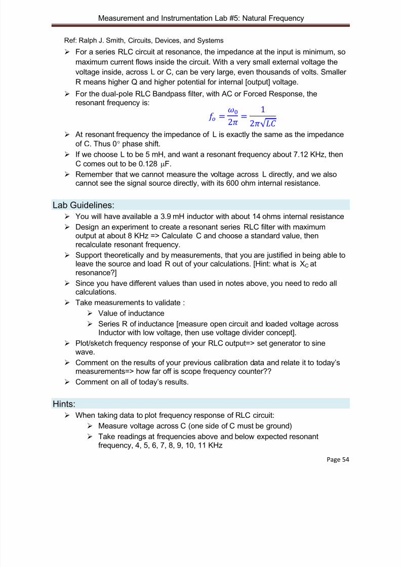
For the dual-pole RLC Bandpass filter, with AC or Forced Response, theresonant frequency is:
At resonant frequency the impedance of L is exactly the same as the impedanceof C. Thus 0° phase shift.
If we choose L to be 5 mH, and want a resonant frequency about 7.12 KHz, thenC comes out to be 0.128 µF.
Remember that we cannot measure the voltage across L directly, and we alsocannot see the signal source directly, with its 600 ohm internal resistance.
Lab Guidelines: You will have available a 3.9 mH inductor with about 14 ohms internal resistance
Design an experiment to create a resonant series RLC filter with maximumoutput at about 8 KHz => Calculate C and choose a standard value, thenrecalculate resonant frequency.
Support theoretically and by measurements, that you are justified in being able toleave the source and load R out of your calculations. [Hint: what is XC atresonance?]
Since you have different values than used in notes above, you need to redo all
calculations. Take measurements to validate :
Value of inductance
Series R of inductance [measure open circuit and loaded voltage acrossInductor with low voltage, then use voltage divider concept].
Plot/sketch frequency response of your RLC output=> set generator to sinewave.
Comment on the results of your previous calibration data and relate it to today’smeasurements=> how far off is scope frequency counter??
Comment on all of today’s results.
Hints: When taking data to plot frequency response of RLC circuit:
Measure voltage across C (one side of C must be ground)
Take readings at frequencies above and below expected resonantfrequency, 4, 5, 6, 7, 8, 9, 10, 11 KHz
=02 =
1
2√

8/13/2019 Lab Textbook (Partial)
http://slidepdf.com/reader/full/lab-textbook-partial 55/68
Measurement and Instrumentation Lab #5: Natural Frequency
Page 55
Then take a few closely spaced readings to further isolate freq. Set scope to measure pk-pk voltage on both input and output, measure
frequency on Capacitor channel, trigger on capacitor channel. AdjustFunction Generator and measure frequency on scope.
Press and release the RUN/STOP button on scope to freeze frame formeasurement (wait few seconds for scan), capture one screen and put in
your lab notebook.
Quick Approximation of L:
Alternate method:
Adjust f to give VL half of VIN, then XL
is about 600 Ω. Measure on scope.
Discuss accuracy.
1. Assume RL is much less than XL and R
2. Set f to 10 KHz so that VL is much greater
than voltage across RL, then measure f and
VIN on oscilloscope with generator open
circuit. (Vpk-pk)
3. Attach inductor (RL + L) and measure V
across inductor, L and R4. VL
2 + VR 2 = VIN 2 (magnitudes)
5. Solve for VR 2 and then VR (600Ω)
6. VL / VR x 600Ω = XL (assuming XL >> R)
7. Solve for L (your answer should be very
close to 3.9 x 10⁻³
H; at 10 kHz, RL is
about 5% of XL, so reduce L calculation
by about 5% and it gets closer to 3.9 mH
and is well within tolerance. To verify
approximation, use 20 kHz and answershould come closer to correct one.) = 2 + ( )2 = 2 + (ω − 1/)2
Voltage and impedance have similar triangles = 2 + ()2

8/13/2019 Lab Textbook (Partial)
http://slidepdf.com/reader/full/lab-textbook-partial 56/68
Measurement and Instrumentation Lab #5: Natural Frequency
Page 56
Frequency Uncertainty for Lab 05 [and 6], all added except for intermediatevalues of L and C. Units are Hz and related to ≈8 KHz.
As part of your uncertainty analysis, you must include printout of graph similar to this in,but with your data. Data must also be listed. Each individual person must have their own
graph with their own name on it. Be sure to save all tables and graphs electronically forreuse in other labs.
Uncertainty Budget for resonant frequency (≈8000Hz):
Source of
Uncertainty
Value (±)
[Hz]
Distribution
Type
Divisor @ 1 Standard
Deviation
Notes
Osc. combined
uncertainty,95%
Normal 2 Referenced to k = 2,
units of Hz
Osc. Resolution
@8KHz, CH1
Rectangular
√ 3 Freq. readout you
used, half of digitbeyond last one
4 cutoff
frequencies
Normal √ 4 Use LabVIEW
L and C Normal 2 L / C tolerance
combined as ratios
Convert above
to Hz @ 8000Hz
Normal 2 Use this one
Combined
uncertainty
Normal 1 sum of squares=>
square rootExpanded
uncertainty
k=2
(x 2)
Approx. 95 %
certainty
Example Report: The measured average value of frequency was 8082.25 Hz ±897.5 Hz,…..Hint: Important Note: Scope “calibration uncertainty” has been transferredto unknown/unmeasured frequencies with assumed conditions that may be……

8/13/2019 Lab Textbook (Partial)
http://slidepdf.com/reader/full/lab-textbook-partial 57/68
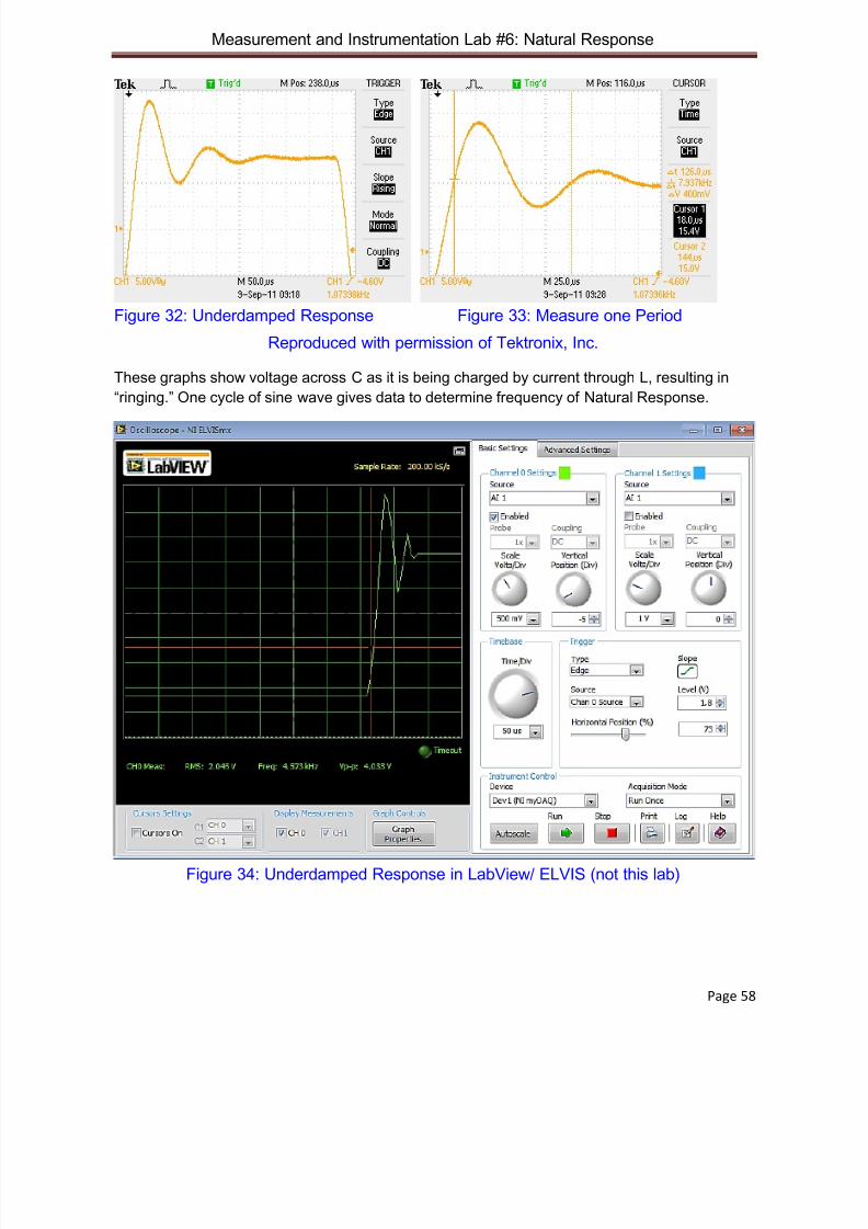
8/13/2019 Lab Textbook (Partial)
http://slidepdf.com/reader/full/lab-textbook-partial 58/68
Measurement and Instrumentation Lab #6: Natural Response
Page 58
Figure 32: Underdamped Response Figure 33: Measure one Period
Reproduced with permission of Tektronix, Inc.
These graphs show voltage across C as it is being charged by current through L, resulting in
“ringing.” One cycle of sine wave gives data to determine frequency of Natural Response.
Figure 34: Underdamped Response in LabView/ ELVIS (not this lab)
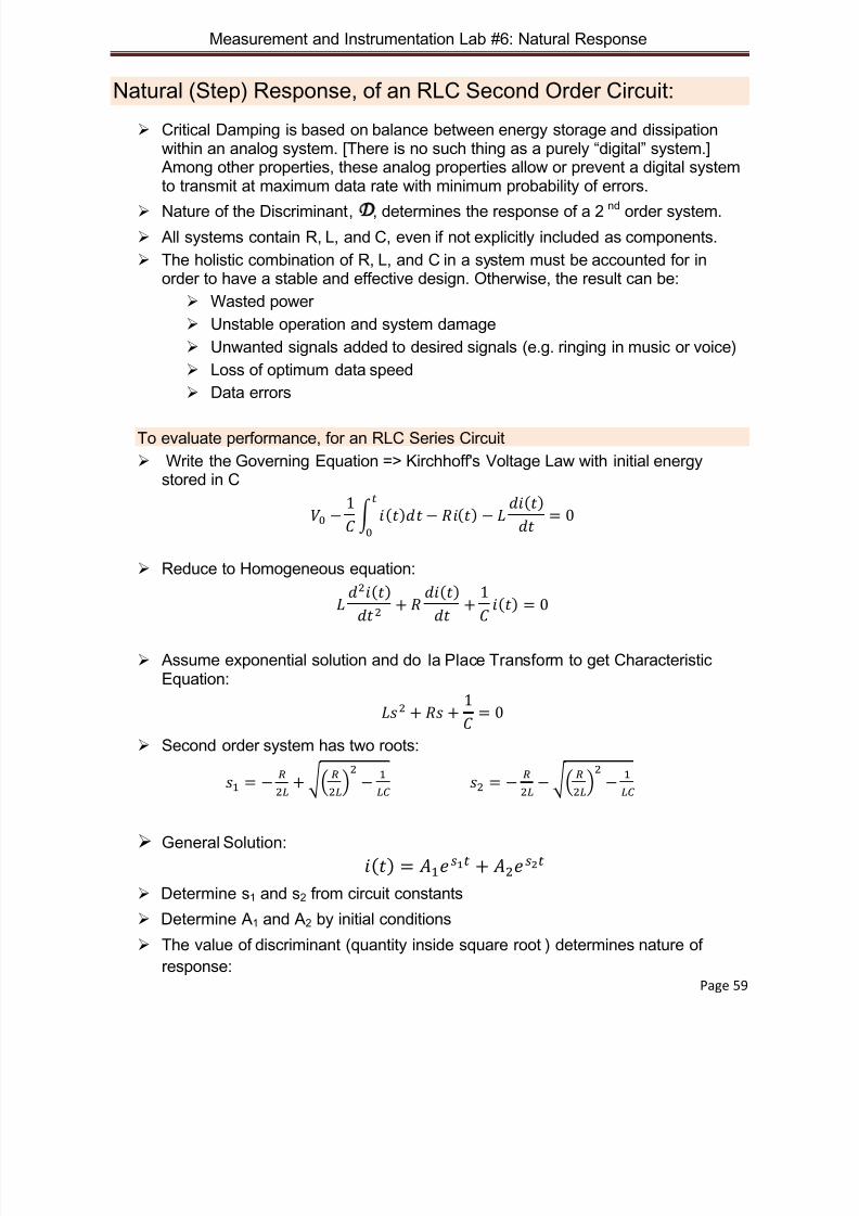
8/13/2019 Lab Textbook (Partial)
http://slidepdf.com/reader/full/lab-textbook-partial 59/68
Measurement and Instrumentation Lab #6: Natural Response
Page 59
Natural (Step) Response, of an RLC Second Order Circuit:
Critical Damping is based on balance between energy storage and dissipationwithin an analog system. [There is no such thing as a purely “digital” system.]Among other properties, these analog properties allow or prevent a digital systemto transmit at maximum data rate with minimum probability of errors.
Nature of the Discriminant, , determines the response of a 2nd order system.
All systems contain R, L, and C, even if not explicitly included as components.
The holistic combination of R, L, and C in a system must be accounted for inorder to have a stable and effective design. Otherwise, the result can be:
Wasted power
Unstable operation and system damage
Unwanted signals added to desired signals (e.g. ringing in music or voice)
Loss of optimum data speed
Data errors
To evaluate performance, for an RLC Series Circuit
Write the Governing Equation => Kirchhoff's Voltage Law with initial energystored in C
0 − 1
() − () − () = 0
0
Reduce to Homogeneous equation:
2()
2+
()
+1
(
) = 0
Assume exponential solution and do la Place Transform to get CharacteristicEquation:
2 + + 1
= 0
Second order system has two roots:
1 = − 2 +
22 − 1
2 = − 2 −
22 − 1
General Solution:
() = 1 + 2 Determine s1 and s2 from circuit constants
Determine A1 and A2 by initial conditions
The value of discriminant (quantity inside square root ) determines nature of
response:
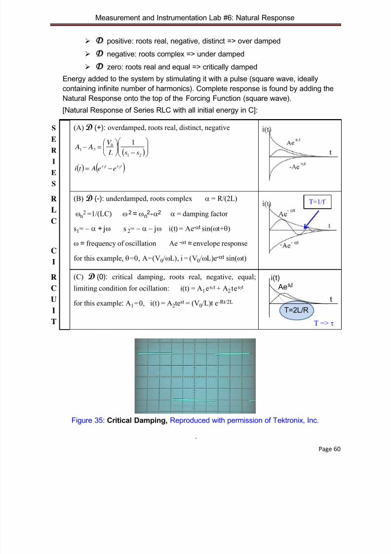
8/13/2019 Lab Textbook (Partial)
http://slidepdf.com/reader/full/lab-textbook-partial 60/68
8/13/2019 Lab Textbook (Partial)
http://slidepdf.com/reader/full/lab-textbook-partial 61/68
Measurement and Instrumentation Lab #6: Natural Response
Page 61
Underdamped Response across C, shown in Fig. 32 and Fig. 33.
Square wave generator is set just slow enough to show entire decay ofoscillation (left graph).
Cursor settings on scope are set to measure period of ringing and convert
it into frequency. Note that left cursor is a little off and real time period islonger/frequency slower.
Lab Guidelines: Part One:
Given an inductor of 3.9 mH, calculate needed C to give resonant[Natural] frequency of 8 KHz, then use standard value.
Assuming your circuit of L and C is underdamped, calculate the“frequency of oscillation” [Natural Response Frequency] and the timeconstant of decay envelope [1/α ≠ period of sine wave].
Before building your circuit and taking measurements, use the above datato predict your response. [as shown in diagram above]
Determine the maximum frequency of square wave needed to displaycircuit response (half period must show 3 cycles of sine wave, setgenerator to 6 x period and explain why)
Take measurements and record your screen shots showing ringing
Part two:
Determine value of resistance that needs to be added to circuit to get
critical damping.4 =
1 (remember the internal R of L)
Choose a resistor close to needed value and measure response Record screen shot showing close to critical damping
Discuss your results, include how close your measured data is to
expected and also implications to a general circuit or system.
Lab Hints:
MyDAQ graph, Fig. 34, give desired result directly because output impedance of
signal generator within MyDAQ is buffered to give one Ω output impedance.
Generators in lab have 600 Ω output impedance, so they will not show ringing
effect if used directly.
Before taking measurements, add 100 Ω resistor in parallel with generator.Calculate Thevenin equivalent new resistance for generator find R “looking into”
generator. [600 Ω in parallel with 100 Ω]
When you calculate series R of RLC circuit, you must include both R of inductor
and Thevenin (new R) of signal generator. This will give you a new frequency of
ringing oscillation of about 7.7 KHz. With component tolerances, this is well
within accuracy of displayed graph.

8/13/2019 Lab Textbook (Partial)
http://slidepdf.com/reader/full/lab-textbook-partial 62/68
Measurement and Instrumentation Lab #6: Natural Response
Page 62
Note that Discriminant graphs shown in table plot current, not voltage. You must
either measure voltage across C alone, or add another series R to circuit and
measure across that to match the graph shape. Otherwise there will be a phase
shift in starting point of graph.
You will need to press cursor button on scope and adjust both cursor 1 and 2 as
shown in Fig. 33, but more accurately.
The following ELVIS function generator setting was used to get Step Response diagram
of Fig. 34
Figure 36: ELVIS Function Generator
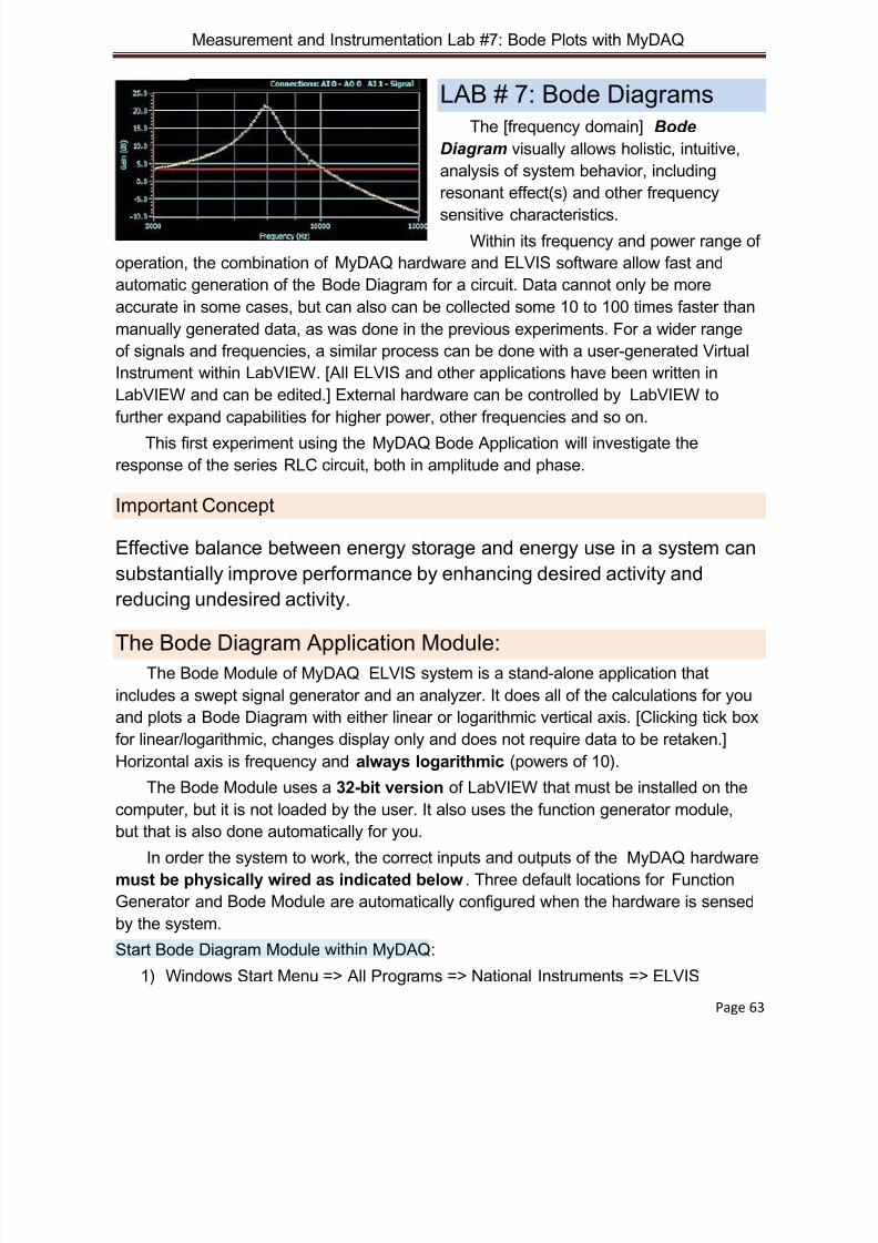
8/13/2019 Lab Textbook (Partial)
http://slidepdf.com/reader/full/lab-textbook-partial 63/68
Measurement and Instrumentation Lab #7: Bode Plots with MyDAQ
Page 63
LAB # 7: Bode DiagramsThe [frequency domain] Bode
Diagram visually allows holistic, intuitive,
analysis of system behavior, including
resonant effect(s) and other frequency
sensitive characteristics.
Within its frequency and power range of
operation, the combination of MyDAQ hardware and ELVIS software allow fast and
automatic generation of the Bode Diagram for a circuit. Data cannot only be more
accurate in some cases, but can also can be collected some 10 to 100 times faster than
manually generated data, as was done in the previous experiments. For a wider range
of signals and frequencies, a similar process can be done with a user-generated Virtual
Instrument within LabVIEW. [All ELVIS and other applications have been written in
LabVIEW and can be edited.] External hardware can be controlled by LabVIEW to
further expand capabilities for higher power, other frequencies and so on.This first experiment using the MyDAQ Bode Application will investigate the
response of the series RLC circuit, both in amplitude and phase.
Important Concept
Effective balance between energy storage and energy use in a system can
substantially improve performance by enhancing desired activity and
reducing undesired activity.
The Bode Diagram Application Module:The Bode Module of MyDAQ ELVIS system is a stand-alone application that
includes a swept signal generator and an analyzer. It does all of the calculations for you
and plots a Bode Diagram with either linear or logarithmic vertical axis. [Clicking tick box
for linear/logarithmic, changes display only and does not require data to be retaken.]
Horizontal axis is frequency and always logarithmic (powers of 10).
The Bode Module uses a 32-bit version of LabVIEW that must be installed on the
computer, but it is not loaded by the user. It also uses the function generator module,
but that is also done automatically for you.
In order the system to work, the correct inputs and outputs of the MyDAQ hardware
must be physically wired as indicated below. Three default locations for Function
Generator and Bode Module are automatically configured when the hardware is sensed
by the system.
Start Bode Diagram Module within MyDAQ:
1) Windows Start Menu => All Programs => National Instruments => ELVIS

8/13/2019 Lab Textbook (Partial)
http://slidepdf.com/reader/full/lab-textbook-partial 64/68
Measurement and Instrumentation Lab #7: Bode Plots with MyDAQ
Page 64
2) Click on NI ELVIS Instrument Launcher
3) When instrument panel comes up, Click on Bode Icon
Wire circuit as shown below, being very careful to make sure that all wires are
making good contact and not touching anything else. Layout is important.
Examples of Bode Plots:
Note differences in linear and dB plots. Also note that signal level is critical. SettingPeak Amplitude too low will result in noisy plots, too high will overload system. Both
give incorrect data.
Figure 37: Linear Mapping (Gain) and 0.20 Volts Peak Amplitude Input
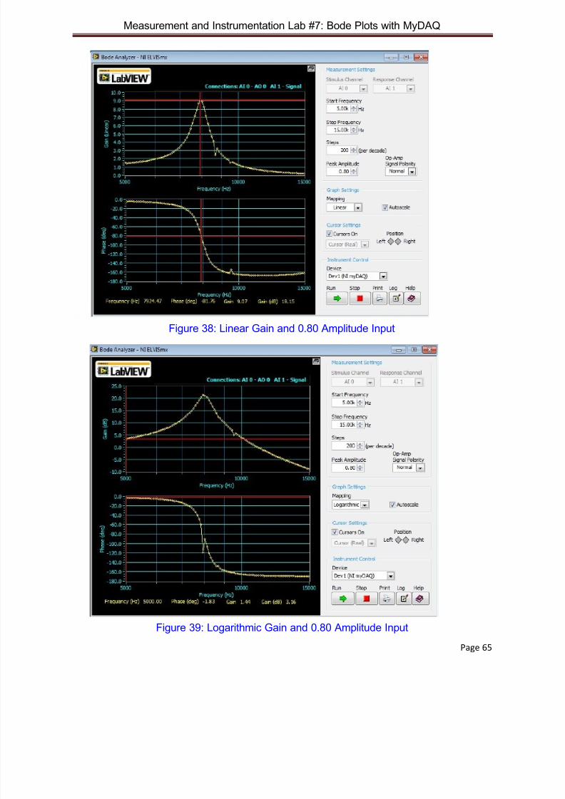
8/13/2019 Lab Textbook (Partial)
http://slidepdf.com/reader/full/lab-textbook-partial 65/68
Measurement and Instrumentation Lab #7: Bode Plots with MyDAQ
Page 65
Figure 38: Linear Gain and 0.80 Amplitude Input
Figure 39: Logarithmic Gain and 0.80 Amplitude Input
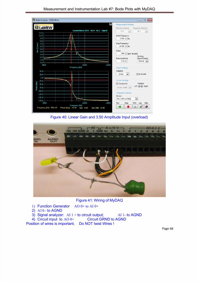
8/13/2019 Lab Textbook (Partial)
http://slidepdf.com/reader/full/lab-textbook-partial 66/68
Measurement and Instrumentation Lab #7: Bode Plots with MyDAQ
Page 66
Figure 40: Linear Gain and 3.50 Amplitude Input (overload)
Figure 41: Wiring of MyDAQ
1) Function Generator AO 0+ to AI 0+2) AI 0 - to AGND3) Signal analyzer: AI 1 + to circuit output; AI 1- to AGND4) Circuit input to AO 0+ Circuit GRND to AGND
Position of wires is important, Do NOT twist Wires !
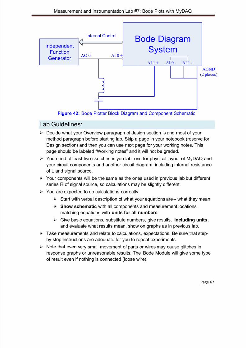
8/13/2019 Lab Textbook (Partial)
http://slidepdf.com/reader/full/lab-textbook-partial 67/68
Measurement and Instrumentation Lab #7: Bode Plots with MyDAQ
Page 67
Independent
Function
Generator
Bode Diagram
SystemAO 0 AI 0 +
AGND
(2 places)
AI 1 -AI 1 +
Internal Control
AI 0 -
Figure 42: Bode Plotter Block Diagram and Component Schematic
Lab Guidelines: Decide what your Overview paragraph of design section is and most of your
method paragraph before starting lab. Skip a page in your notebook (reserve for
Design section) and then you can use next page for your working notes. This
page should be labeled “Working notes” and it will not be graded.
You need at least two sketches in you lab, one for physical layout of MyDAQ and
your circuit components and another circuit diagram, including internal resistance
of L and signal source.
Your components will be the same as the ones used in previous lab but differentseries R of signal source, so calculations may be slightly different.
You are expected to do calculations correctly:
Start with verbal description of what your equations are – what they mean
Show schematic with all components and measurement locations
matching equations with units for all numbers
Give basic equations, substitute numbers, give results, including units,
and evaluate what results mean, show on graphs as in previous lab.
Take measurements and relate to calculations, expectations. Be sure that step-
by-step instructions are adequate for you to repeat experiments.
Note that even very small movement of parts or wires may cause glitches in
response graphs or unreasonable results. The Bode Module will give some type
of result even if nothing is connected (loose wire).

8/13/2019 Lab Textbook (Partial)
http://slidepdf.com/reader/full/lab-textbook-partial 68/68