Embed Size (px)
Citation preview

Lab7: Nonlinear Regression and OBDecomposition in R
Introduction to Econometrics,Fall 2021
Feifan Wang
Nanjing University
11/04/2021
Feifan Wang (Nanjing University) Lab7: Nonlinear Regression and OB Decomposition in R11/04/2021 1 / 44
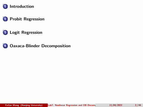
1 Introduction
2 Probit Regression
3 Logit Regression
4 Oaxaca-Blinder Decomposition
Feifan Wang (Nanjing University) Lab7: Nonlinear Regression and OB Decomposition in R11/04/2021 2 / 44

library(tidyverse)library(magrittr)library(haven)library(ggplot2)library(AER) # package of Applied Econonometrics in Rlibrary(stargazer)
Feifan Wang (Nanjing University) Lab7: Nonlinear Regression and OB Decomposition in R11/04/2021 3 / 44

Section 1
Introduction
Feifan Wang (Nanjing University) Lab7: Nonlinear Regression and OB Decomposition in R11/04/2021 4 / 44

Regression with a Binary Dependent Variable
Type Population regression function(I) LPM 𝑃(𝑌𝑖 = 1|𝑋𝑖) = 𝛽0 + 𝛽1𝑋𝑖 + 𝑢𝑖(II) Probit 𝐸(𝑌 |𝑋) = 𝑃 (𝑌 = 1|𝑋) = Φ(𝛽0 + 𝛽1𝑋)(III) Logit 𝐸(𝑌 |𝑋) = 𝑃 (𝑌 = 1|𝑋) = 𝐹(𝛽0 + 𝛽1𝑋)
Feifan Wang (Nanjing University) Lab7: Nonlinear Regression and OB Decomposition in R11/04/2021 5 / 44

Data: HMDAFollowing the book, we start by loading the data set HMDA whichprovides data that relate to mortgage applications filed in Boston inthe year of 1990.
data(HMDA)head(HMDA)
## deny pirat hirat lvrat chist mhist phist unemp selfemp insurance condomin## 1 no 0.221 0.221 0.8000000 5 2 no 3.9 no no no## 2 no 0.265 0.265 0.9218750 2 2 no 3.2 no no no## 3 no 0.372 0.248 0.9203980 1 2 no 3.2 no no no## 4 no 0.320 0.250 0.8604651 1 2 no 4.3 no no no## 5 no 0.360 0.350 0.6000000 1 1 no 3.2 no no no## 6 no 0.240 0.170 0.5105263 1 1 no 3.9 no no no## afam single hschool## 1 no no yes## 2 no yes yes## 3 no no yes## 4 no no yes## 5 no no yes## 6 no no yes
Feifan Wang (Nanjing University) Lab7: Nonlinear Regression and OB Decomposition in R11/04/2021 6 / 44
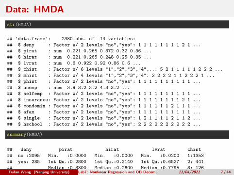
Data: HMDAstr(HMDA)
## 'data.frame': 2380 obs. of 14 variables:## $ deny : Factor w/ 2 levels "no","yes": 1 1 1 1 1 1 1 1 2 1 ...## $ pirat : num 0.221 0.265 0.372 0.32 0.36 ...## $ hirat : num 0.221 0.265 0.248 0.25 0.35 ...## $ lvrat : num 0.8 0.922 0.92 0.86 0.6 ...## $ chist : Factor w/ 6 levels "1","2","3","4",..: 5 2 1 1 1 1 1 2 2 2 ...## $ mhist : Factor w/ 4 levels "1","2","3","4": 2 2 2 2 1 1 2 2 2 1 ...## $ phist : Factor w/ 2 levels "no","yes": 1 1 1 1 1 1 1 1 1 1 ...## $ unemp : num 3.9 3.2 3.2 4.3 3.2 ...## $ selfemp : Factor w/ 2 levels "no","yes": 1 1 1 1 1 1 1 1 1 1 ...## $ insurance: Factor w/ 2 levels "no","yes": 1 1 1 1 1 1 1 1 2 1 ...## $ condomin : Factor w/ 2 levels "no","yes": 1 1 1 1 1 1 2 1 1 1 ...## $ afam : Factor w/ 2 levels "no","yes": 1 1 1 1 1 1 1 1 1 1 ...## $ single : Factor w/ 2 levels "no","yes": 1 2 1 1 1 1 2 1 1 2 ...## $ hschool : Factor w/ 2 levels "no","yes": 2 2 2 2 2 2 2 2 2 2 ...
summary(HMDA)
## deny pirat hirat lvrat chist## no :2095 Min. :0.0000 Min. :0.0000 Min. :0.0200 1:1353## yes: 285 1st Qu.:0.2800 1st Qu.:0.2140 1st Qu.:0.6527 2: 441## Median :0.3300 Median :0.2600 Median :0.7795 3: 126## Mean :0.3308 Mean :0.2553 Mean :0.7378 4: 77## 3rd Qu.:0.3700 3rd Qu.:0.2988 3rd Qu.:0.8685 5: 182## Max. :3.0000 Max. :3.0000 Max. :1.9500 6: 201## mhist phist unemp selfemp insurance condomin## 1: 747 no :2205 Min. : 1.800 no :2103 no :2332 no :1694## 2:1571 yes: 175 1st Qu.: 3.100 yes: 277 yes: 48 yes: 686## 3: 41 Median : 3.200## 4: 21 Mean : 3.774## 3rd Qu.: 3.900## Max. :10.600## afam single hschool## no :2041 no :1444 no : 39## yes: 339 yes: 936 yes:2341########
#HMDA<- HMDA %>% filter(pirat<=1)
Feifan Wang (Nanjing University) Lab7: Nonlinear Regression and OB Decomposition in R11/04/2021 7 / 44

Data: HMDA
The variable we are interested in is deny, an indicator for whether anapplicant’s mortgage application has been accepted (deny = "no")or denied (deny = "yes").
A regressor that ought to have power in explaining whether amortgage application has been denied is pirat, which is the ratio ofthe payment to household income.
𝑑𝑒𝑛𝑦 = 𝛽0 + 𝛽1 × 𝑃/𝐼 𝑟𝑎𝑡𝑖𝑜 + 𝑢 (1)
Feifan Wang (Nanjing University) Lab7: Nonlinear Regression and OB Decomposition in R11/04/2021 8 / 44

Data: HMDA
The variable we are interested in is deny, an indicator for whether anapplicant’s mortgage application has been accepted (deny = "no")or denied (deny = "yes").A regressor that ought to have power in explaining whether amortgage application has been denied is pirat, which is the ratio ofthe payment to household income.
𝑑𝑒𝑛𝑦 = 𝛽0 + 𝛽1 × 𝑃/𝐼 𝑟𝑎𝑡𝑖𝑜 + 𝑢 (1)
Feifan Wang (Nanjing University) Lab7: Nonlinear Regression and OB Decomposition in R11/04/2021 8 / 44
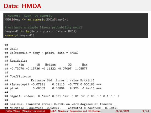
Data: HMDA# convert 'deny' to numericHMDA$deny <- as.numeric(HMDA$deny)-1
# estimate a simple linear probability modeldenymod1 <- lm(deny ~ pirat, data = HMDA)summary(denymod1)
#### Call:## lm(formula = deny ~ pirat, data = HMDA)#### Residuals:## Min 1Q Median 3Q Max## -0.73070 -0.13736 -0.11322 -0.07097 1.05577#### Coefficients:## Estimate Std. Error t value Pr(>|t|)## (Intercept) -0.07991 0.02116 -3.777 0.000163 ***## pirat 0.60353 0.06084 9.920 < 2e-16 ***## ---## Signif. codes: 0 '***' 0.001 '**' 0.01 '*' 0.05 '.' 0.1 ' ' 1#### Residual standard error: 0.3183 on 2378 degrees of freedom## Multiple R-squared: 0.03974, Adjusted R-squared: 0.03933## F-statistic: 98.41 on 1 and 2378 DF, p-value: < 2.2e-16Feifan Wang (Nanjing University) Lab7: Nonlinear Regression and OB Decomposition in R11/04/2021 9 / 44

Predicted Probability
# plot the dataplot(x = HMDA$pirat,
y = HMDA$deny,xlab = "P/I ratio",ylab = "Deny",pch = 20,ylim = c(-0.4, 1.4),cex.main = 0.8)
# add horizontal dashed lines and textabline(h = 1, lty = 2, col = "darkred")abline(h = 0, lty = 2, col = "darkred")text(2.5, 0.9, cex = 0.8, "Mortgage denied")text(2.5, -0.1, cex= 0.8, "Mortgage approved")
# add the estimated regression lineabline(denymod1,
lwd = 1.8,col = "red")
Feifan Wang (Nanjing University) Lab7: Nonlinear Regression and OB Decomposition in R11/04/2021 10 / 44

Predicted Probability
0.0 0.5 1.0 1.5 2.0 2.5 3.0
0.0
0.5
1.0
Scatterplot Mortgage Application Denial and the Payment−to−Income Ratio
P/I ratio
Den
y
Mortgage denied
Mortgage approved
Feifan Wang (Nanjing University) Lab7: Nonlinear Regression and OB Decomposition in R11/04/2021 11 / 44

Linear probabilty model: Black v.s White
# estimate a simple linear probability modeldenymod2 <- lm(deny ~ pirat+afam,data = HMDA)coeftest(denymod2, vcov. = vcovHC, type = "HC1")
#### t test of coefficients:#### Estimate Std. Error t value Pr(>|t|)## (Intercept) -0.090514 0.028600 -3.1649 0.001571 **## pirat 0.559195 0.088666 6.3067 3.387e-10 ***## afamyes 0.177428 0.024946 7.1124 1.502e-12 ***## ---## Signif. codes: 0 '***' 0.001 '**' 0.01 '*' 0.05 '.' 0.1 ' ' 1
Feifan Wang (Nanjing University) Lab7: Nonlinear Regression and OB Decomposition in R11/04/2021 12 / 44

Section 2
Probit Regression
Feifan Wang (Nanjing University) Lab7: Nonlinear Regression and OB Decomposition in R11/04/2021 13 / 44

Probit Regression
In Probit regression, the cumulative standard normal distributionfunction Φ(⋅) is used to model the regression function when thedependent variable is binary
𝐸(𝑌 |𝑋) = 𝑃 (𝑌 = 1|𝑋) = Φ(𝛽0 + 𝛽1𝑋)
Feifan Wang (Nanjing University) Lab7: Nonlinear Regression and OB Decomposition in R11/04/2021 14 / 44
Probit Regression
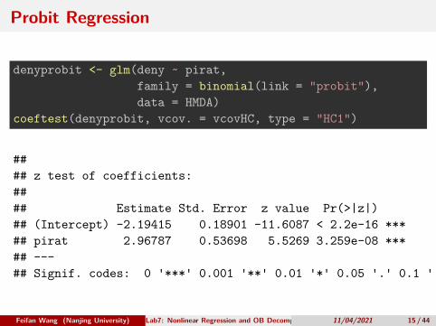
denyprobit <- glm(deny ~ pirat,family = binomial(link = "probit"),data = HMDA)
coeftest(denyprobit, vcov. = vcovHC, type = "HC1")
#### z test of coefficients:#### Estimate Std. Error z value Pr(>|z|)## (Intercept) -2.19415 0.18901 -11.6087 < 2.2e-16 ***## pirat 2.96787 0.53698 5.5269 3.259e-08 ***## ---## Signif. codes: 0 '***' 0.001 '**' 0.01 '*' 0.05 '.' 0.1 ' ' 1
Feifan Wang (Nanjing University) Lab7: Nonlinear Regression and OB Decomposition in R11/04/2021 15 / 44

Predicted Probability
# plot dataplot(x = HMDA$pirat,
y = HMDA$deny,main = "Probit Model of the Probability of Denial, Given P/I Ratio",xlab = "P/I ratio",ylab = "Deny",pch = 20,ylim = c(-0.4, 1.4),cex.main = 0.85)
# add horizontal dashed lines and textabline(h = 1, lty = 2, col = "darkred")abline(h = 0, lty = 2, col = "darkred")text(2.5, 0.9, cex = 0.8, "Mortgage denied")text(2.5, -0.1, cex= 0.8, "Mortgage approved")
# add estimated regression linex <- seq(0, 3, 0.01)y <- predict(denyprobit, list(pirat = x), type = "response")
lines(x, y, lwd = 1.5, col = "steelblue")
Feifan Wang (Nanjing University) Lab7: Nonlinear Regression and OB Decomposition in R11/04/2021 16 / 44

Predicted Probability
0.0 0.5 1.0 1.5 2.0 2.5 3.0
0.0
0.5
1.0
Probit Model of the Probability of Denial, Given P/I Ratio
P/I ratio
Den
y
Mortgage denied
Mortgage approved
Feifan Wang (Nanjing University) Lab7: Nonlinear Regression and OB Decomposition in R11/04/2021 17 / 44

Prediction differences
# 1. compute predictions for P/I ratio = 0.3, 0.4predictions <- predict(denyprobit,
newdata = data.frame("pirat" = c(0.3, 0.4)),type = "response")
# 2. Compute difference in probabilitiesdiff(predictions)
## 2## 0.06081433
Feifan Wang (Nanjing University) Lab7: Nonlinear Regression and OB Decomposition in R11/04/2021 18 / 44

Probit Regression:Black v.s White
denyprobit2 <- glm(deny ~ pirat + afam,family = binomial(link = "probit"),data = HMDA)
coeftest(denyprobit2, vcov. = vcovHC, type = "HC1")
#### z test of coefficients:#### Estimate Std. Error z value Pr(>|z|)## (Intercept) -2.258787 0.176608 -12.7898 < 2.2e-16 ***## pirat 2.741779 0.497673 5.5092 3.605e-08 ***## afamyes 0.708155 0.083091 8.5227 < 2.2e-16 ***## ---## Signif. codes: 0 '***' 0.001 '**' 0.01 '*' 0.05 '.' 0.1 ' ' 1
Feifan Wang (Nanjing University) Lab7: Nonlinear Regression and OB Decomposition in R11/04/2021 19 / 44

Black v.s White
# 1. compute predictions for P/I ratio = 0.3predictions <- predict(denyprobit2,
newdata = data.frame("afam" = c("no", "yes"),"pirat" = c(0.3, 0.3)),type = "response")
# 2. compute difference in probabilitiesdiff(predictions)
## 2## 0.1578117
Feifan Wang (Nanjing University) Lab7: Nonlinear Regression and OB Decomposition in R11/04/2021 20 / 44

Section 3
Logit Regression
Feifan Wang (Nanjing University) Lab7: Nonlinear Regression and OB Decomposition in R11/04/2021 21 / 44

Logit Regression
In Logit regression, the cumulative logistic distribution function 𝐹(⋅)is used to model the regression function when the dependent variableis binary
𝐸(𝑌 |𝑋) = 𝑃(𝑌 = 1|𝑋) = 𝐹(𝛽0 + 𝛽1𝑋)
Feifan Wang (Nanjing University) Lab7: Nonlinear Regression and OB Decomposition in R11/04/2021 22 / 44

Logit Regression
denylogit <- glm(deny ~ pirat,family = binomial(link = "logit"),data = HMDA)
coeftest(denylogit, vcov. = vcovHC, type = "HC1")
#### z test of coefficients:#### Estimate Std. Error z value Pr(>|z|)## (Intercept) -4.02843 0.35898 -11.2218 < 2.2e-16 ***## pirat 5.88450 1.00015 5.8836 4.014e-09 ***## ---## Signif. codes: 0 '***' 0.001 '**' 0.01 '*' 0.05 '.' 0.1 ' ' 1
Feifan Wang (Nanjing University) Lab7: Nonlinear Regression and OB Decomposition in R11/04/2021 23 / 44

Predicted Probability# plot dataplot(x = HMDA$pirat,
y = HMDA$deny,main = "Probit and Logit Models Model of the Probability of Denial, Given P/I Ratio",xlab = "P/I ratio",ylab = "Deny",pch = 20,ylim = c(-0.4, 1.4),cex.main = 0.9)
# add horizontal dashed lines and textabline(h = 1, lty = 2, col = "darkred")abline(h = 0, lty = 2, col = "darkred")text(2.5, 0.9, cex = 0.8, "Mortgage denied")text(2.5, -0.1, cex= 0.8, "Mortgage approved")
# add estimated regression line of Probit and Logit modelsx <- seq(0, 3, 0.01)y_probit <- predict(denyprobit, list(pirat = x), type = "response")y_logit <- predict(denylogit, list(pirat = x), type = "response")
lines(x, y_probit, lwd = 1.5, col = "steelblue")lines(x, y_logit, lwd = 1.5, col = "black", lty = 2)
# add a legendlegend("topleft",
horiz = TRUE,legend = c("Probit", "Logit"),col = c("steelblue", "black"),lty = c(1, 2))
Feifan Wang (Nanjing University) Lab7: Nonlinear Regression and OB Decomposition in R11/04/2021 24 / 44

Predicted Probability
0.0 0.5 1.0 1.5 2.0 2.5 3.0
0.0
0.5
1.0
Probit and Logit Models Model of the Probability of Denial, Given P/I Ratio
P/I ratio
Den
y
Mortgage denied
Mortgage approved
Probit Logit
Feifan Wang (Nanjing University) Lab7: Nonlinear Regression and OB Decomposition in R11/04/2021 25 / 44

Logit Regression: White vs Black
# estimate a Logit regression with multiple regressorsdenylogit2 <- glm(deny ~ pirat + afam,
family = binomial(link = "logit"),data = HMDA)
coeftest(denylogit2, vcov. = vcovHC, type = "HC1")
#### z test of coefficients:#### Estimate Std. Error z value Pr(>|z|)## (Intercept) -4.12556 0.34597 -11.9245 < 2.2e-16 ***## pirat 5.37036 0.96376 5.5723 2.514e-08 ***## afamyes 1.27278 0.14616 8.7081 < 2.2e-16 ***## ---## Signif. codes: 0 '***' 0.001 '**' 0.01 '*' 0.05 '.' 0.1 ' ' 1
Feifan Wang (Nanjing University) Lab7: Nonlinear Regression and OB Decomposition in R11/04/2021 26 / 44

Logit Regression: White vs Black
# 1. compute predictions for P/I ratio = 0.3predictions <- predict(denylogit2,
newdata = data.frame("afam" = c("no", "yes"),"pirat" = c(0.3, 0.3)),type = "response")
predictions
## 1 2## 0.07485143 0.22414592
# 2. Compute difference in probabilitiesdiff(predictions)
## 2## 0.1492945
Feifan Wang (Nanjing University) Lab7: Nonlinear Regression and OB Decomposition in R11/04/2021 27 / 44

Table 11.2
# estimate all 6 models for the denial probability
lpm_HMDA <- lm(deny ~ afam + pirat + hirat + lvrat + chist + mhist + phist+ insurance + selfemp, data = HMDA)
logit_HMDA <- glm(deny ~ afam + pirat + hirat + lvrat + chist + mhist + phist+ insurance + selfemp,family = binomial(link = "logit"),data = HMDA)
probit_HMDA_1 <- glm(deny ~ afam + pirat + hirat + lvrat + chist + mhist + phist+ insurance + selfemp,family = binomial(link = "probit"),data = HMDA)
Feifan Wang (Nanjing University) Lab7: Nonlinear Regression and OB Decomposition in R11/04/2021 28 / 44

Table 11.2
probit_HMDA_2 <- glm(deny ~ afam + pirat + hirat + lvrat + chist + mhist + phist+ insurance + selfemp + single + hschool + unemp,family = binomial(link = "probit"),data = HMDA)
probit_HMDA_3 <- glm(deny ~ afam + pirat + hirat + lvrat + chist + mhist+ phist + insurance + selfemp + single + hschool + unemp + condomin+ I(mhist==3) + I(mhist==4) + I(chist==3) + I(chist==4) + I(chist==5)+ I(chist==6), family = binomial(link = "probit"),data = HMDA)
probit_HMDA_4 <- glm(deny ~ afam * (pirat + hirat) + lvrat + chist + mhist + phist+ insurance + selfemp + single + hschool + unemp,family = binomial(link = "probit"),data = HMDA)
Feifan Wang (Nanjing University) Lab7: Nonlinear Regression and OB Decomposition in R11/04/2021 29 / 44

Table 11.2
rob_se <- list(sqrt(diag(vcovHC(lpm_HMDA, type = "HC1"))),sqrt(diag(vcovHC(logit_HMDA, type = "HC1"))),sqrt(diag(vcovHC(probit_HMDA_1, type = "HC1"))),sqrt(diag(vcovHC(probit_HMDA_2, type = "HC1"))),sqrt(diag(vcovHC(probit_HMDA_3, type = "HC1"))),sqrt(diag(vcovHC(probit_HMDA_4, type = "HC1"))))
stargazer(lpm_HMDA, logit_HMDA, probit_HMDA_1,probit_HMDA_2, probit_HMDA_3, probit_HMDA_4,digits = 3,type = "latex",header = FALSE,se = rob_se,model.numbers = FALSE,column.labels = c("(1)", "(2)", "(3)", "(4)", "(5)", "(6)"))
Feifan Wang (Nanjing University) Lab7: Nonlinear Regression and OB Decomposition in R11/04/2021 30 / 44

Table 11.2Mortgage Denial Regressions
Dependent Variable: deny=1 if application is denied,=0 if acceptedOLS logistic probit(1) (2) (3) (4) (5) (6)
afamyes 0.087∗∗∗ 0.684∗∗∗ 0.386∗∗∗ 0.374∗∗∗ 0.380∗∗∗ 0.284(0.022) (0.177) (0.097) (0.098) (0.099) (0.492)
pirat 0.483∗∗∗ 5.135∗∗∗ 2.648∗∗∗ 2.644∗∗∗ 2.653∗∗∗ 2.756∗∗∗(0.115) (1.358) (0.677) (0.659) (0.658) (0.726)
hirat −0.077 −0.666 −0.442 −0.522 −0.546 −0.738(0.111) (1.338) (0.709) (0.705) (0.705) (0.762)
lvrat 0.090∗∗ 1.776∗∗∗ 0.754∗∗ 0.780∗∗ 0.784∗∗ 0.775∗∗(0.037) (0.623) (0.339) (0.336) (0.335) (0.337)
chist2 0.040∗∗∗ 0.708∗∗∗ 0.324∗∗∗ 0.324∗∗∗ 0.322∗∗∗ 0.324∗∗∗(0.015) (0.209) (0.105) (0.106) (0.107) (0.106)
chist3 0.051 0.882∗∗∗ 0.449∗∗∗ 0.434∗∗ 0.432∗∗ 0.435∗∗(0.032) (0.327) (0.173) (0.175) (0.175) (0.174)
chist4 0.142∗∗∗ 1.581∗∗∗ 0.793∗∗∗ 0.764∗∗∗ 0.769∗∗∗ 0.755∗∗∗(0.044) (0.317) (0.173) (0.182) (0.182) (0.182)
chist5 0.106∗∗∗ 1.207∗∗∗ 0.602∗∗∗ 0.609∗∗∗ 0.608∗∗∗ 0.610∗∗∗(0.028) (0.233) (0.122) (0.120) (0.120) (0.120)
chist6 0.159∗∗∗ 1.491∗∗∗ 0.778∗∗∗ 0.799∗∗∗ 0.800∗∗∗ 0.803∗∗∗(0.032) (0.236) (0.128) (0.129) (0.129) (0.130)
mhist2 0.027∗∗ 0.426∗∗ 0.221∗∗ 0.165 0.166 0.166(0.012) (0.201) (0.102) (0.105) (0.105) (0.105)
mhist3 0.042 0.549 0.279 0.209 0.207 0.210(0.061) (0.502) (0.271) (0.271) (0.272) (0.273)
mhist4 0.033 0.578 0.272 0.234 0.231 0.240(0.081) (0.607) (0.339) (0.353) (0.353) (0.354)
phistyes 0.204∗∗∗ 1.268∗∗∗ 0.723∗∗∗ 0.724∗∗∗ 0.724∗∗∗ 0.726∗∗∗(0.035) (0.201) (0.114) (0.115) (0.115) (0.114)
insuranceyes 0.713∗∗∗ 4.565∗∗∗ 2.551∗∗∗ 2.576∗∗∗ 2.574∗∗∗ 2.581∗∗∗(0.044) (0.582) (0.304) (0.299) (0.299) (0.300)
selfempyes 0.061∗∗∗ 0.670∗∗∗ 0.352∗∗∗ 0.337∗∗∗ 0.337∗∗∗ 0.339∗∗∗(0.021) (0.213) (0.113) (0.115) (0.115) (0.115)
singleyes 0.230∗∗∗ 0.237∗∗∗ 0.227∗∗∗(0.081) (0.085) (0.082)
hschoolyes −0.552∗∗ −0.558∗∗ −0.560∗∗(0.239) (0.239) (0.239)
unemp 0.031∗ 0.031∗ 0.031∗(0.018) (0.018) (0.018)
condominyes −0.035(0.094)
I(mhist == 3)
I(mhist == 4)
I(chist == 3)
I(chist == 4)
I(chist == 5)
I(chist == 6)
afamyes:pirat −0.634(1.545)
afamyes:hirat 1.177(1.737)
Constant −0.191∗∗∗ −6.471∗∗∗ −3.298∗∗∗ −2.936∗∗∗ −2.922∗∗∗ −2.905∗∗∗(0.030) (0.617) (0.321) (0.395) (0.399) (0.406)
Observations 2,380 2,380 2,380 2,380 2,380 2,380Adjusted R2 0.254Log Likelihood −636.641 −639.472 −631.707 −631.633 −631.455Akaike Inf. Crit. 1,305.282 1,310.944 1,301.415 1,303.265 1,304.909Residual Std. Error 0.280
Note: ∗p<0.1; ∗∗p<0.05; ∗∗∗p<0.01Robust S.E. are shown in the parentheses
Feifan Wang (Nanjing University) Lab7: Nonlinear Regression and OB Decomposition in R11/04/2021 31 / 44
Section 4
Oaxaca-Blinder Decomposition
Feifan Wang (Nanjing University) Lab7: Nonlinear Regression and OB Decomposition in R11/04/2021 32 / 44
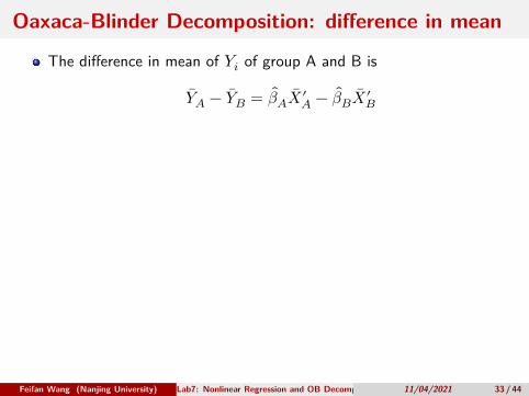
Oaxaca-Blinder Decomposition: difference in mean
The difference in mean of 𝑌𝑖 of group A and B is
𝑌𝐴 − 𝑌𝐵 = 𝛽𝐴��′𝐴 − 𝛽𝐵��′
𝐵
A small trick: plus and minus a term 𝛽𝐵��′𝐴,then
𝑌𝐴 − 𝑌𝐵 = 𝛽𝐴��′𝐴 − 𝛽𝐵��′
𝐵
= 𝛽𝐴��′𝐴 − 𝛽𝐵��′
𝐴 + 𝛽𝐵��′𝐴 − 𝛽𝐵��′
𝐵
= ( 𝛽𝐴 − 𝛽𝐵)��′𝐴 + 𝛽𝐵(��′
𝐴 − ��′𝐵)
Then the second term is characteristics effect which describes howmuch the difference of outcome, 𝑌 , in mean is due to differences inthe levels of explanatory variables(characteristics).the first term is coefficients effect which describes how much thedifference of outcome, 𝑌 , in mean is due to differences in themagnitude of regression coefficients.
Feifan Wang (Nanjing University) Lab7: Nonlinear Regression and OB Decomposition in R11/04/2021 33 / 44
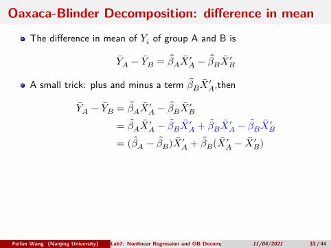

Oaxaca-Blinder Decomposition: difference in mean
The difference in mean of 𝑌𝑖 of group A and B is
𝑌𝐴 − 𝑌𝐵 = 𝛽𝐴��′𝐴 − 𝛽𝐵��′
𝐵
A small trick: plus and minus a term 𝛽𝐵��′𝐴,then
𝑌𝐴 − 𝑌𝐵 = 𝛽𝐴��′𝐴 − 𝛽𝐵��′
𝐵
= 𝛽𝐴��′𝐴 − 𝛽𝐵��′
𝐴 + 𝛽𝐵��′𝐴 − 𝛽𝐵��′
𝐵
= ( 𝛽𝐴 − 𝛽𝐵)��′𝐴 + 𝛽𝐵(��′
𝐴 − ��′𝐵)
Then the second term is characteristics effect which describes howmuch the difference of outcome, 𝑌 , in mean is due to differences inthe levels of explanatory variables(characteristics).
the first term is coefficients effect which describes how much thedifference of outcome, 𝑌 , in mean is due to differences in themagnitude of regression coefficients.
Feifan Wang (Nanjing University) Lab7: Nonlinear Regression and OB Decomposition in R11/04/2021 33 / 44

Oaxaca-Blinder Decomposition: difference in mean
The difference in mean of 𝑌𝑖 of group A and B is
𝑌𝐴 − 𝑌𝐵 = 𝛽𝐴��′𝐴 − 𝛽𝐵��′
𝐵
A small trick: plus and minus a term 𝛽𝐵��′𝐴,then
𝑌𝐴 − 𝑌𝐵 = 𝛽𝐴��′𝐴 − 𝛽𝐵��′
𝐵
= 𝛽𝐴��′𝐴 − 𝛽𝐵��′
𝐴 + 𝛽𝐵��′𝐴 − 𝛽𝐵��′
𝐵
= ( 𝛽𝐴 − 𝛽𝐵)��′𝐴 + 𝛽𝐵(��′
𝐴 − ��′𝐵)
Then the second term is characteristics effect which describes howmuch the difference of outcome, 𝑌 , in mean is due to differences inthe levels of explanatory variables(characteristics).the first term is coefficients effect which describes how much thedifference of outcome, 𝑌 , in mean is due to differences in themagnitude of regression coefficients.
Feifan Wang (Nanjing University) Lab7: Nonlinear Regression and OB Decomposition in R11/04/2021 33 / 44

Oaxaca-Blinder Decomposition: a general framework
Then the difference of the potential outcomes between two groupscan then be decomposed as follows
𝑌𝐴 − 𝑌𝐵 = ��′𝐴 𝛽𝐴 − ��′
𝐵 𝛽𝐵
= ��′𝐴 𝛽𝐴 − ��′
𝐴 𝛽∗ + ��′𝐴 𝛽∗−��′
𝐵 𝛽∗ + ��′𝐵 𝛽∗−��′
𝐵 𝛽𝐵
= (��′𝐴 − ��′
𝐵) 𝛽∗ + [��′𝐴( 𝛽𝐴 − 𝛽∗) + ��′
𝐵( 𝛽∗− 𝛽𝐵)]
Feifan Wang (Nanjing University) Lab7: Nonlinear Regression and OB Decomposition in R11/04/2021 34 / 44

Oaxaca-Blinder Decomposition: a general framework
The first term, (��′𝐴 − ��′
𝐵) 𝛽∗ is the explained part as usual
characteristics effectendownment effectcomposition effect
The second term, the unexplained part can further be subdividedinto
1 “discrimination” in favor of group A(such as Men)
��′𝐴( 𝛽𝐴 − 𝛽∗)
2 “discrimination” against group B(such as Women)
��′𝐵( 𝛽∗ − 𝛽𝐵)
Feifan Wang (Nanjing University) Lab7: Nonlinear Regression and OB Decomposition in R11/04/2021 35 / 44

Oaxaca-Blinder Decomposition: a general framework
The first term, (��′𝐴 − ��′
𝐵) 𝛽∗ is the explained part as usualcharacteristics effect
endownment effectcomposition effect
The second term, the unexplained part can further be subdividedinto
1 “discrimination” in favor of group A(such as Men)
��′𝐴( 𝛽𝐴 − 𝛽∗)
2 “discrimination” against group B(such as Women)
��′𝐵( 𝛽∗ − 𝛽𝐵)
Feifan Wang (Nanjing University) Lab7: Nonlinear Regression and OB Decomposition in R11/04/2021 35 / 44

Oaxaca-Blinder Decomposition: a general framework
The first term, (��′𝐴 − ��′
𝐵) 𝛽∗ is the explained part as usualcharacteristics effectendownment effect
composition effectThe second term, the unexplained part can further be subdividedinto
1 “discrimination” in favor of group A(such as Men)
��′𝐴( 𝛽𝐴 − 𝛽∗)
2 “discrimination” against group B(such as Women)
��′𝐵( 𝛽∗ − 𝛽𝐵)
Feifan Wang (Nanjing University) Lab7: Nonlinear Regression and OB Decomposition in R11/04/2021 35 / 44

Oaxaca-Blinder Decomposition: a general framework
The first term, (��′𝐴 − ��′
𝐵) 𝛽∗ is the explained part as usualcharacteristics effectendownment effectcomposition effect
The second term, the unexplained part can further be subdividedinto
1 “discrimination” in favor of group A(such as Men)
��′𝐴( 𝛽𝐴 − 𝛽∗)
2 “discrimination” against group B(such as Women)
��′𝐵( 𝛽∗ − 𝛽𝐵)
Feifan Wang (Nanjing University) Lab7: Nonlinear Regression and OB Decomposition in R11/04/2021 35 / 44

Oaxaca-Blinder Decomposition: a general framework
The first term, (��′𝐴 − ��′
𝐵) 𝛽∗ is the explained part as usualcharacteristics effectendownment effectcomposition effect
The second term, the unexplained part can further be subdividedinto
1 “discrimination” in favor of group A(such as Men)
��′𝐴( 𝛽𝐴 − 𝛽∗)
2 “discrimination” against group B(such as Women)
��′𝐵( 𝛽∗ − 𝛽𝐵)
Feifan Wang (Nanjing University) Lab7: Nonlinear Regression and OB Decomposition in R11/04/2021 35 / 44

Install Packages
#install.packages("oaxaca")library(oaxaca)
Feifan Wang (Nanjing University) Lab7: Nonlinear Regression and OB Decomposition in R11/04/2021 36 / 44
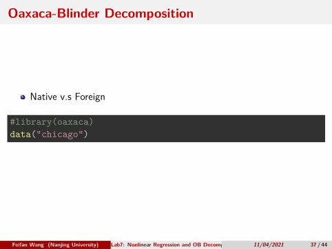
Oaxaca-Blinder Decomposition
Native v.s Foreign
#library(oaxaca)data("chicago")
Feifan Wang (Nanjing University) Lab7: Nonlinear Regression and OB Decomposition in R11/04/2021 37 / 44
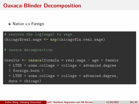
Oaxaca-Blinder Decomposition
Native v.s Foreign
# restore the log(wage) to wagechicago$real.wage <- exp(chicago$ln.real.wage)
# oaxaca decomposition
results <- oaxaca(formula = real.wage ~ age + female+ LTHS + some.college + college + advanced.degree| foreign.born |+ LTHS + some.college + college + advanced.degree,data = chicago)
Feifan Wang (Nanjing University) Lab7: Nonlinear Regression and OB Decomposition in R11/04/2021 38 / 44

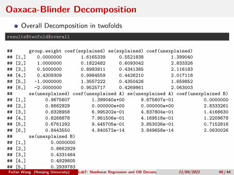
Oaxaca-Blinder DecompositionOverall Decomposition in twofolds
results$twofold$overall
## group.weight coef(explained) se(explained) coef(unexplained)## [1,] 0.0000000 1.6165339 0.5521838 1.399040## [2,] 1.0000000 0.1822482 0.6093042 2.833326## [3,] 0.5000000 0.8993911 0.4341385 2.116183## [4,] 0.4309309 0.9984559 0.4426210 2.017118## [5,] -1.0000000 1.3557222 0.4350426 1.659852## [6,] -2.0000000 0.9525717 0.4269861 2.063003## se(unexplained) coef(unexplained A) se(unexplained A) coef(unexplained B)## [1,] 0.9675607 1.399040e+00 9.675607e-01 0.0000000## [2,] 0.8662929 0.000000e+00 0.000000e+00 2.8333261## [3,] 0.8328958 6.995202e-01 4.837804e-01 1.4166630## [4,] 0.8268878 7.961506e-01 4.169518e-01 1.2209678## [5,] 0.6761292 9.445705e-01 3.853026e-01 0.7152816## [6,] 0.8443550 4.840572e-14 3.849658e-14 2.0630026## se(unexplained B)## [1,] 0.0000000## [2,] 0.8662929## [3,] 0.4331464## [4,] 0.4929805## [5,] 0.2939783## [6,] 0.8443550Feifan Wang (Nanjing University) Lab7: Nonlinear Regression and OB Decomposition in R11/04/2021 39 / 44
Oaxaca-Blinder DecompositionOverall Decomposition in twofolds
results$twofold$overall
## group.weight coef(explained) se(explained) coef(unexplained)## [1,] 0.0000000 1.6165339 0.5521838 1.399040## [2,] 1.0000000 0.1822482 0.6093042 2.833326## [3,] 0.5000000 0.8993911 0.4341385 2.116183## [4,] 0.4309309 0.9984559 0.4426210 2.017118## [5,] -1.0000000 1.3557222 0.4350426 1.659852## [6,] -2.0000000 0.9525717 0.4269861 2.063003## se(unexplained) coef(unexplained A) se(unexplained A) coef(unexplained B)## [1,] 0.9675607 1.399040e+00 9.675607e-01 0.0000000## [2,] 0.8662929 0.000000e+00 0.000000e+00 2.8333261## [3,] 0.8328958 6.995202e-01 4.837804e-01 1.4166630## [4,] 0.8268878 7.961506e-01 4.169518e-01 1.2209678## [5,] 0.6761292 9.445705e-01 3.853026e-01 0.7152816## [6,] 0.8443550 4.840572e-14 3.849658e-14 2.0630026## se(unexplained B)## [1,] 0.0000000## [2,] 0.8662929## [3,] 0.4331464## [4,] 0.4929805## [5,] 0.2939783## [6,] 0.8443550Feifan Wang (Nanjing University) Lab7: Nonlinear Regression and OB Decomposition in R11/04/2021 40 / 44

Oaxaca-Blinder DecompositionDetailed Decomposition in twofolds
results$twofold$variables
## [[1]]## group.weight coef(explained) se(explained) coef(unexplained)## (Intercept) 0 0.00000000 0.0000000 -4.26374940## age 0 -0.51677529 0.1942235 6.32615876## female 0 -0.27265166 0.1587495 -1.41569495## LTHS 0 2.17644672 0.4047570 0.01973059## some.college 0 -0.78533521 0.3981989 0.19816994## college 0 -0.07907587 0.1081671 0.91805037## advanced.degree 0 0.70631440 0.3476113 -0.59276551## (Base) 0 0.38761084 0.1929361 0.20914055## se(unexplained) coef(unexplained A) se(unexplained A)## (Intercept) 2.5027463 -4.26374940 2.5027463## age 1.7737915 6.32615876 1.7737915## female 0.7161933 -1.41569495 0.7161933## LTHS 0.1950737 0.01973059 0.1950737## some.college 0.7565703 0.19816994 0.7565703## college 0.4307505 0.91805037 0.4307505## advanced.degree 0.4160289 -0.59276551 0.4160289## (Base) 0.5461521 0.20914055 0.5461521## coef(unexplained B) se(unexplained B)## (Intercept) 0 0## age 0 0## female 0 0## LTHS 0 0## some.college 0 0## college 0 0## advanced.degree 0 0## (Base) 0 0#### [[2]]## group.weight coef(explained) se(explained) coef(unexplained)## (Intercept) 1 0.0000000 0.0000000 -4.26374940## age 1 -1.7491472 0.4394072 7.55853070## female 1 -0.5230820 0.2850904 -1.16526457## LTHS 1 2.1315790 0.3672828 0.06459830## some.college 1 -0.6561142 0.2782319 0.06894895## college 1 0.2565104 0.1716329 0.58246411## advanced.degree 1 0.3828740 0.1598105 -0.26932512## (Base) 1 0.3396283 0.2081567 0.25712310## se(unexplained) coef(unexplained A) se(unexplained A)## (Intercept) 2.5027463 0 0## age 2.1870992 0 0## female 0.5578858 0 0## LTHS 0.6372269 0 0## some.college 0.2716997 0 0## college 0.2579248 0 0## advanced.degree 0.1961789 0 0## (Base) 0.6575533 0 0## coef(unexplained B) se(unexplained B)## (Intercept) -4.26374940 2.5027463## age 7.55853070 2.1870992## female -1.16526457 0.5578858## LTHS 0.06459830 0.6372269## some.college 0.06894895 0.2716997## college 0.58246411 0.2579248## advanced.degree -0.26932512 0.1961789## (Base) 0.25712310 0.6575533#### [[3]]## group.weight coef(explained) se(explained) coef(unexplained)## (Intercept) 0.5 0.00000000 0.00000000 -4.26374940## age 0.5 -1.13296126 0.25431565 6.94234473## female 0.5 -0.39786685 0.20786399 -1.29047976## LTHS 0.5 2.15401287 0.31581236 0.04216444## some.college 0.5 -0.72072472 0.24026635 0.13355945## college 0.5 0.08871727 0.07873703 0.75025724## advanced.degree 0.5 0.54459421 0.23716962 -0.43104531## (Base) 0.5 0.36361957 0.19043804 0.23313182## se(unexplained) coef(unexplained A) se(unexplained A)## (Intercept) 2.5027463 -2.131874701 1.25137313## age 1.9784199 3.163079379 0.88689573## female 0.6340766 -0.707847475 0.35809667## LTHS 0.4152481 0.009865293 0.09753686## some.college 0.5126889 0.099084970 0.37828515## college 0.3341499 0.459025187 0.21537527## advanced.degree 0.2980705 -0.296382754 0.20801445## (Base) 0.6010982 0.104570274 0.27307604## coef(unexplained B) se(unexplained B)## (Intercept) -2.13187470 1.25137313## age 3.77926535 1.09354959## female -0.58263229 0.27894288## LTHS 0.03229915 0.31861347## some.college 0.03447448 0.13584983## college 0.29123205 0.12896239## advanced.degree -0.13466256 0.09808947## (Base) 0.12856155 0.32877663#### [[4]]## group.weight coef(explained) se(explained) coef(unexplained)## (Intercept) 0.4309309 0.00000000 0.00000000 -4.26374940## age 0.4309309 -1.04784248 0.27635967 6.85722595## female 0.4309309 -0.38056985 0.21742106 -1.30777675## LTHS 0.4309309 2.15711184 0.31414347 0.03906547## some.college 0.4309309 -0.72964989 0.23080922 0.14248462## college 0.4309309 0.06553863 0.08775204 0.77343587## advanced.degree 0.4309309 0.56693394 0.22358609 -0.45338504## (Base) 0.4309309 0.36693368 0.19174156 0.22981771## se(unexplained) coef(unexplained A) se(unexplained A)## (Intercept) 2.5027463 -2.42636790 1.0785108## age 2.0070336 3.60002128 0.7643816## female 0.6231482 -0.80562821 0.3086299## LTHS 0.4458650 0.01122807 0.0840633## some.college 0.4791278 0.11277238 0.3260295## college 0.3220402 0.52243407 0.1856237## advanced.degree 0.2826180 -0.33732452 0.1792797## (Base) 0.6088164 0.11901542 0.2353538## coef(unexplained B) se(unexplained B)## (Intercept) -1.83738150 1.4242355## age 3.25720467 1.2446105## female -0.50214855 0.3174755## LTHS 0.02783741 0.3626261## some.college 0.02971224 0.1546159## college 0.25100180 0.1467770## advanced.degree -0.11606052 0.1116394## (Base) 0.11080230 0.3741932#### [[5]]## group.weight coef(explained) se(explained) coef(unexplained)## (Intercept) -1 0.0000000 0.0000000 -4.26374940## age -1 -0.9077617 0.1889496 6.71714514## female -1 -0.3765153 0.1924727 -1.31183132## LTHS -1 2.2842920 0.3395741 -0.08811472## some.college -1 -0.6457845 0.2298420 0.05861926## college -1 0.1184423 0.1020764 0.72053222## advanced.degree -1 0.5247323 0.2098660 -0.41118338## (Base) -1 0.3583171 0.1890215 0.23843424## se(unexplained) coef(unexplained A) se(unexplained A)## (Intercept) 2.5027463 -2.79648002 1.37592503## age 1.9117128 4.31910081 1.23066863## female 0.6495781 -0.82854887 0.43750585## LTHS 0.4543170 0.06715558 0.09887232## some.college 0.4566300 -0.01584134 0.30285648## college 0.3194437 0.37770759 0.18035670## advanced.degree 0.2718542 -0.25998201 0.15930891## (Base) 0.6070087 0.08145872 0.26198287## coef(unexplained B) se(unexplained B)## (Intercept) -1.4672694 1.3393762## age 2.3980443 0.8476843## female -0.4832824 0.2455140## LTHS -0.1552703 0.3887881## some.college 0.0744606 0.1762796## college 0.3428246 0.1456698## advanced.degree -0.1512014 0.1156621## (Base) 0.1569755 0.3812108#### [[6]]## group.weight coef(explained) se(explained) coef(unexplained)## (Intercept) -2 0.000000e+00 0.000000e+00 -4.2637494## age -2 -1.022467e+00 2.109268e-01 6.8318508## female -2 -3.827757e-01 2.023125e-01 -1.3055709## LTHS -2 7.719266e-01 1.816907e-01 1.4242507## some.college -2 5.306534e-01 2.375042e-01 -1.1178187## college -2 3.494225e-01 1.992421e-01 0.4895520## advanced.degree -2 7.058122e-01 2.777488e-01 -0.5922633## (Base) -2 -1.110223e-16 1.114487e-16 0.5967514## se(unexplained) coef(unexplained A) se(unexplained A)## (Intercept) 2.5027463 1.8071336 1.3836825## age 1.9310723 3.7302801 1.1410953## female 0.6452018 -0.7931584 0.4145636## LTHS 0.5226847 -0.5979074 0.1458423## some.college 0.5018208 -1.8199959 0.3957505## college 0.3145956 -0.2541760 0.1693892## advanced.degree 0.3071787 -0.5918452 0.2203823## (Base) 0.5917146 -1.4803309 0.3355536## coef(unexplained B) se(unexplained B)## (Intercept) -6.0708830237 1.8621860## age 3.1015706708 0.8977154## female -0.5124125091 0.2527662## LTHS 2.0221581467 0.4993462## some.college 0.7021772181 0.2579598## college 0.7437280111 0.2002168## advanced.degree -0.0004181581 0.1041770## (Base) 2.0770822578 0.5012035
Feifan Wang (Nanjing University) Lab7: Nonlinear Regression and OB Decomposition in R11/04/2021 41 / 44
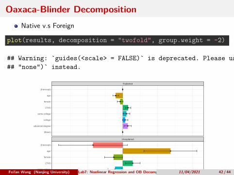
Oaxaca-Blinder DecompositionNative v.s Foreign
plot(results, decomposition = "twofold", group.weight = -2)
## Warning: `guides(<scale> = FALSE)` is deprecated. Please use `guides(<scale> =## "none")` instead.
Unexplained
Explained
−10 −5 0 5 10
(Base)
advanced.degree
college
some.college
LTHS
female
age
(Intercept)
(Base)
advanced.degree
college
some.college
LTHS
female
age
(Intercept)
Feifan Wang (Nanjing University) Lab7: Nonlinear Regression and OB Decomposition in R11/04/2021 42 / 44

Oaxaca-Blinder Decompositionprint(results)
## $beta## $beta$beta.A## (Intercept) age female LTHS some.college## 13.5813773 0.2640051 -6.1497192 -7.9124405 -2.6016154## college advanced.degree## 5.4431146 10.0692349#### $beta$beta.B## (Intercept) age female LTHS some.college## 17.84512667 0.07799874 -3.20548407 -8.07898985 -3.11400069## college advanced.degree## -1.67797882 18.57541990#### $beta$beta.diff## (Intercept) age female LTHS some.college## -4.2637494 0.1860063 -2.9442351 0.1665494 0.5123853## college advanced.degree## 7.1210934 -8.5061850#### $beta$beta.R## (Intercept) age female LTHS some.college## [1,] 0.0000000 17.84513 0.07799874 -3.205484 -8.078990 -3.114001## [2,] 1.0000000 13.58138 0.26400505 -6.149719 -7.912440 -2.601615## [3,] 0.5000000 15.71325 0.17100190 -4.677602 -7.995715 -2.857808## [4,] 0.4309309 16.00775 0.15815462 -4.474246 -8.007219 -2.893198## [5,] -1.0000000 16.37786 0.13701172 -4.426578 -8.479313 -2.560656## [6,] -2.0000000 11.77424 0.15432465 -4.500180 -2.865398 2.104140## college advanced.degree## [1,] -1.677979 18.57542## [2,] 5.443115 10.06923## [3,] 1.882568 14.32233## [4,] 1.390721 14.90984## [5,] 2.513329 13.79998## [6,] 7.414696 18.56221###### $call## oaxaca(formula = real.wage ~ age + female + LTHS + some.college +## college + advanced.degree | foreign.born | +LTHS + some.college +## college + advanced.degree, data = chicago)#### $n## $n$n.A## [1] 287#### $n$n.B## [1] 379#### $n$n.pooled## [1] 666###### $R## [1] 100#### $reg## $reg$reg.A#### Call:## NULL#### Coefficients:## (Intercept) age female LTHS## 8.583 0.264 -6.150 -2.914## some.college college advanced.degree## 2.397 10.441 15.068###### $reg$reg.B#### Call:## NULL#### Coefficients:## (Intercept) age female LTHS## 12.141 0.078 -3.205 -2.375## some.college college advanced.degree## 2.590 4.026 24.280###### $reg$reg.pooled.1#### Call:## NULL#### Coefficients:## (Intercept) age female LTHS## 11.105 0.137 -4.427 -3.206## some.college college advanced.degree## 2.713 7.787 19.073###### $reg$reg.pooled.2#### Call:## NULL#### Coefficients:## (Intercept) age female LTHS## 11.7742 0.1543 -4.5002 -2.8654## some.college college advanced.degree foreign.born## 2.1041 7.4147 18.5622 -2.0630######## $threefold## $threefold$overall## coef(endowments) se(endowments) coef(coefficients) se(coefficients)## 1.6165339 0.5521838 2.8333261 0.8662929## coef(interaction) se(interaction)## -1.4342857 0.7735712#### $threefold$variables## coef(endowments) se(endowments) coef(coefficients)## (Intercept) 0.00000000 0.0000000 -4.26374940## age -0.51677529 0.1942235 7.55853070## female -0.27265166 0.1587495 -1.16526457## LTHS 2.17644672 0.4047570 0.06459830## some.college -0.78533521 0.3981989 0.06894895## college -0.07907587 0.1081671 0.58246411## advanced.degree 0.70631440 0.3476113 -0.26932512## (Base) 0.38761084 0.1929361 0.25712310## se(coefficients) coef(interaction) se(interaction)## (Intercept) 2.5027463 0.00000000 0.0000000## age 2.1870992 -1.23237194 0.4504410## female 0.5578858 -0.25043038 0.2003149## LTHS 0.6372269 -0.04486771 0.4455334## some.college 0.2716997 0.12922099 0.4909572## college 0.2579248 0.33558627 0.2398288## advanced.degree 0.1961789 -0.32344039 0.2602851## (Base) 0.6575533 -0.04798255 0.1266511###### $twofold## $twofold$overall## group.weight coef(explained) se(explained) coef(unexplained)## [1,] 0.0000000 1.6165339 0.5521838 1.399040## [2,] 1.0000000 0.1822482 0.6093042 2.833326## [3,] 0.5000000 0.8993911 0.4341385 2.116183## [4,] 0.4309309 0.9984559 0.4426210 2.017118## [5,] -1.0000000 1.3557222 0.4350426 1.659852## [6,] -2.0000000 0.9525717 0.4269861 2.063003## se(unexplained) coef(unexplained A) se(unexplained A) coef(unexplained B)## [1,] 0.9675607 1.399040e+00 9.675607e-01 0.0000000## [2,] 0.8662929 0.000000e+00 0.000000e+00 2.8333261## [3,] 0.8328958 6.995202e-01 4.837804e-01 1.4166630## [4,] 0.8268878 7.961506e-01 4.169518e-01 1.2209678## [5,] 0.6761292 9.445705e-01 3.853026e-01 0.7152816## [6,] 0.8443550 4.840572e-14 3.849658e-14 2.0630026## se(unexplained B)## [1,] 0.0000000## [2,] 0.8662929## [3,] 0.4331464## [4,] 0.4929805## [5,] 0.2939783## [6,] 0.8443550#### $twofold$variables## $twofold$variables[[1]]## group.weight coef(explained) se(explained) coef(unexplained)## (Intercept) 0 0.00000000 0.0000000 -4.26374940## age 0 -0.51677529 0.1942235 6.32615876## female 0 -0.27265166 0.1587495 -1.41569495## LTHS 0 2.17644672 0.4047570 0.01973059## some.college 0 -0.78533521 0.3981989 0.19816994## college 0 -0.07907587 0.1081671 0.91805037## advanced.degree 0 0.70631440 0.3476113 -0.59276551## (Base) 0 0.38761084 0.1929361 0.20914055## se(unexplained) coef(unexplained A) se(unexplained A)## (Intercept) 2.5027463 -4.26374940 2.5027463## age 1.7737915 6.32615876 1.7737915## female 0.7161933 -1.41569495 0.7161933## LTHS 0.1950737 0.01973059 0.1950737## some.college 0.7565703 0.19816994 0.7565703## college 0.4307505 0.91805037 0.4307505## advanced.degree 0.4160289 -0.59276551 0.4160289## (Base) 0.5461521 0.20914055 0.5461521## coef(unexplained B) se(unexplained B)## (Intercept) 0 0## age 0 0## female 0 0## LTHS 0 0## some.college 0 0## college 0 0## advanced.degree 0 0## (Base) 0 0#### $twofold$variables[[2]]## group.weight coef(explained) se(explained) coef(unexplained)## (Intercept) 1 0.0000000 0.0000000 -4.26374940## age 1 -1.7491472 0.4394072 7.55853070## female 1 -0.5230820 0.2850904 -1.16526457## LTHS 1 2.1315790 0.3672828 0.06459830## some.college 1 -0.6561142 0.2782319 0.06894895## college 1 0.2565104 0.1716329 0.58246411## advanced.degree 1 0.3828740 0.1598105 -0.26932512## (Base) 1 0.3396283 0.2081567 0.25712310## se(unexplained) coef(unexplained A) se(unexplained A)## (Intercept) 2.5027463 0 0## age 2.1870992 0 0## female 0.5578858 0 0## LTHS 0.6372269 0 0## some.college 0.2716997 0 0## college 0.2579248 0 0## advanced.degree 0.1961789 0 0## (Base) 0.6575533 0 0## coef(unexplained B) se(unexplained B)## (Intercept) -4.26374940 2.5027463## age 7.55853070 2.1870992## female -1.16526457 0.5578858## LTHS 0.06459830 0.6372269## some.college 0.06894895 0.2716997## college 0.58246411 0.2579248## advanced.degree -0.26932512 0.1961789## (Base) 0.25712310 0.6575533#### $twofold$variables[[3]]## group.weight coef(explained) se(explained) coef(unexplained)## (Intercept) 0.5 0.00000000 0.00000000 -4.26374940## age 0.5 -1.13296126 0.25431565 6.94234473## female 0.5 -0.39786685 0.20786399 -1.29047976## LTHS 0.5 2.15401287 0.31581236 0.04216444## some.college 0.5 -0.72072472 0.24026635 0.13355945## college 0.5 0.08871727 0.07873703 0.75025724## advanced.degree 0.5 0.54459421 0.23716962 -0.43104531## (Base) 0.5 0.36361957 0.19043804 0.23313182## se(unexplained) coef(unexplained A) se(unexplained A)## (Intercept) 2.5027463 -2.131874701 1.25137313## age 1.9784199 3.163079379 0.88689573## female 0.6340766 -0.707847475 0.35809667## LTHS 0.4152481 0.009865293 0.09753686## some.college 0.5126889 0.099084970 0.37828515## college 0.3341499 0.459025187 0.21537527## advanced.degree 0.2980705 -0.296382754 0.20801445## (Base) 0.6010982 0.104570274 0.27307604## coef(unexplained B) se(unexplained B)## (Intercept) -2.13187470 1.25137313## age 3.77926535 1.09354959## female -0.58263229 0.27894288## LTHS 0.03229915 0.31861347## some.college 0.03447448 0.13584983## college 0.29123205 0.12896239## advanced.degree -0.13466256 0.09808947## (Base) 0.12856155 0.32877663#### $twofold$variables[[4]]## group.weight coef(explained) se(explained) coef(unexplained)## (Intercept) 0.4309309 0.00000000 0.00000000 -4.26374940## age 0.4309309 -1.04784248 0.27635967 6.85722595## female 0.4309309 -0.38056985 0.21742106 -1.30777675## LTHS 0.4309309 2.15711184 0.31414347 0.03906547## some.college 0.4309309 -0.72964989 0.23080922 0.14248462## college 0.4309309 0.06553863 0.08775204 0.77343587## advanced.degree 0.4309309 0.56693394 0.22358609 -0.45338504## (Base) 0.4309309 0.36693368 0.19174156 0.22981771## se(unexplained) coef(unexplained A) se(unexplained A)## (Intercept) 2.5027463 -2.42636790 1.0785108## age 2.0070336 3.60002128 0.7643816## female 0.6231482 -0.80562821 0.3086299## LTHS 0.4458650 0.01122807 0.0840633## some.college 0.4791278 0.11277238 0.3260295## college 0.3220402 0.52243407 0.1856237## advanced.degree 0.2826180 -0.33732452 0.1792797## (Base) 0.6088164 0.11901542 0.2353538## coef(unexplained B) se(unexplained B)## (Intercept) -1.83738150 1.4242355## age 3.25720467 1.2446105## female -0.50214855 0.3174755## LTHS 0.02783741 0.3626261## some.college 0.02971224 0.1546159## college 0.25100180 0.1467770## advanced.degree -0.11606052 0.1116394## (Base) 0.11080230 0.3741932#### $twofold$variables[[5]]## group.weight coef(explained) se(explained) coef(unexplained)## (Intercept) -1 0.0000000 0.0000000 -4.26374940## age -1 -0.9077617 0.1889496 6.71714514## female -1 -0.3765153 0.1924727 -1.31183132## LTHS -1 2.2842920 0.3395741 -0.08811472## some.college -1 -0.6457845 0.2298420 0.05861926## college -1 0.1184423 0.1020764 0.72053222## advanced.degree -1 0.5247323 0.2098660 -0.41118338## (Base) -1 0.3583171 0.1890215 0.23843424## se(unexplained) coef(unexplained A) se(unexplained A)## (Intercept) 2.5027463 -2.79648002 1.37592503## age 1.9117128 4.31910081 1.23066863## female 0.6495781 -0.82854887 0.43750585## LTHS 0.4543170 0.06715558 0.09887232## some.college 0.4566300 -0.01584134 0.30285648## college 0.3194437 0.37770759 0.18035670## advanced.degree 0.2718542 -0.25998201 0.15930891## (Base) 0.6070087 0.08145872 0.26198287## coef(unexplained B) se(unexplained B)## (Intercept) -1.4672694 1.3393762## age 2.3980443 0.8476843## female -0.4832824 0.2455140## LTHS -0.1552703 0.3887881## some.college 0.0744606 0.1762796## college 0.3428246 0.1456698## advanced.degree -0.1512014 0.1156621## (Base) 0.1569755 0.3812108#### $twofold$variables[[6]]## group.weight coef(explained) se(explained) coef(unexplained)## (Intercept) -2 0.000000e+00 0.000000e+00 -4.2637494## age -2 -1.022467e+00 2.109268e-01 6.8318508## female -2 -3.827757e-01 2.023125e-01 -1.3055709## LTHS -2 7.719266e-01 1.816907e-01 1.4242507## some.college -2 5.306534e-01 2.375042e-01 -1.1178187## college -2 3.494225e-01 1.992421e-01 0.4895520## advanced.degree -2 7.058122e-01 2.777488e-01 -0.5922633## (Base) -2 -1.110223e-16 1.114487e-16 0.5967514## se(unexplained) coef(unexplained A) se(unexplained A)## (Intercept) 2.5027463 1.8071336 1.3836825## age 1.9310723 3.7302801 1.1410953## female 0.6452018 -0.7931584 0.4145636## LTHS 0.5226847 -0.5979074 0.1458423## some.college 0.5018208 -1.8199959 0.3957505## college 0.3145956 -0.2541760 0.1693892## advanced.degree 0.3071787 -0.5918452 0.2203823## (Base) 0.5917146 -1.4803309 0.3355536## coef(unexplained B) se(unexplained B)## (Intercept) -6.0708830237 1.8621860## age 3.1015706708 0.8977154## female -0.5124125091 0.2527662## LTHS 2.0221581467 0.4993462## some.college 0.7021772181 0.2579598## college 0.7437280111 0.2002168## advanced.degree -0.0004181581 0.1041770## (Base) 2.0770822578 0.5012035######## $x## $x$x.mean.A## (Intercept) age female LTHS some.college## 1.00000000 34.01045296 0.48083624 0.11846690 0.38675958## college advanced.degree## 0.12891986 0.06968641#### $x$x.mean.B## (Intercept) age female LTHS some.college## 1.00000000 40.63588391 0.39577836 0.38786280 0.13456464## college advanced.degree## 0.08179420 0.03166227#### $x$x.mean.diff## (Intercept) age female LTHS some.college## 0.00000000 -6.62543094 0.08505787 -0.26939590 0.25219494## college advanced.degree## 0.04712567 0.03802414###### $y## $y$y.A## [1] 17.58282#### $y$y.B## [1] 14.56725#### $y$y.diff## [1] 3.015574###### attr(,"class")## [1] "oaxaca"
Feifan Wang (Nanjing University) Lab7: Nonlinear Regression and OB Decomposition in R11/04/2021 43 / 44

Oaxaca-Blinder Decomposition: Exercise
Calculate the share of overall endowment effect to wage gapbetween natives and foreign borns
Calculate the share of overall price effect to wage gap betweennatives and foreign bornCalculate shares of detailed endownment effects(every independentvariable) to wage gap between natives and foreign bornsCalculate the share of detailed price effect(every independentvariable plus constant) to wage gap between natives and foreign bornsShow all desirable results above in a table using Stargazer or Kablepackages
Feifan Wang (Nanjing University) Lab7: Nonlinear Regression and OB Decomposition in R11/04/2021 44 / 44

Oaxaca-Blinder Decomposition: Exercise
Calculate the share of overall endowment effect to wage gapbetween natives and foreign bornsCalculate the share of overall price effect to wage gap betweennatives and foreign born
Calculate shares of detailed endownment effects(every independentvariable) to wage gap between natives and foreign bornsCalculate the share of detailed price effect(every independentvariable plus constant) to wage gap between natives and foreign bornsShow all desirable results above in a table using Stargazer or Kablepackages
Feifan Wang (Nanjing University) Lab7: Nonlinear Regression and OB Decomposition in R11/04/2021 44 / 44

Oaxaca-Blinder Decomposition: Exercise
Calculate the share of overall endowment effect to wage gapbetween natives and foreign bornsCalculate the share of overall price effect to wage gap betweennatives and foreign bornCalculate shares of detailed endownment effects(every independentvariable) to wage gap between natives and foreign borns
Calculate the share of detailed price effect(every independentvariable plus constant) to wage gap between natives and foreign bornsShow all desirable results above in a table using Stargazer or Kablepackages
Feifan Wang (Nanjing University) Lab7: Nonlinear Regression and OB Decomposition in R11/04/2021 44 / 44

Oaxaca-Blinder Decomposition: Exercise
Calculate the share of overall endowment effect to wage gapbetween natives and foreign bornsCalculate the share of overall price effect to wage gap betweennatives and foreign bornCalculate shares of detailed endownment effects(every independentvariable) to wage gap between natives and foreign bornsCalculate the share of detailed price effect(every independentvariable plus constant) to wage gap between natives and foreign borns
Show all desirable results above in a table using Stargazer or Kablepackages
Feifan Wang (Nanjing University) Lab7: Nonlinear Regression and OB Decomposition in R11/04/2021 44 / 44

Oaxaca-Blinder Decomposition: Exercise
Calculate the share of overall endowment effect to wage gapbetween natives and foreign bornsCalculate the share of overall price effect to wage gap betweennatives and foreign bornCalculate shares of detailed endownment effects(every independentvariable) to wage gap between natives and foreign bornsCalculate the share of detailed price effect(every independentvariable plus constant) to wage gap between natives and foreign bornsShow all desirable results above in a table using Stargazer or Kablepackages
Feifan Wang (Nanjing University) Lab7: Nonlinear Regression and OB Decomposition in R11/04/2021 44 / 44