Labor-Leisure Choice

Labor-Leisure Choice

Lecture 8 Labor-Leisure Choice 1 / 24

Utility Maximization

utility= u(C, L), (C is the amount of goods and services consumed, and L isthe amount of leisure)

Budget constraint is PC =WH+ y0 (P is price of consumption goods; W iswage rate; H is hours worked; y0 is unearned income)

Time constraint is H+ L= T (T is time endowment)

Eliminate H to get full budget constraint:

PC+WL=WT + y0

left-hand-side is total cost of “commodities”

right-hand-side is “full income”

increase in W raises the price of leisure and raises full income


Budget Line and Indifference Curves


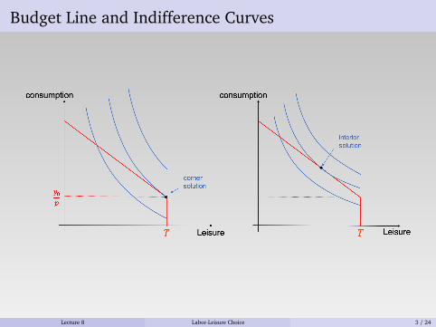
Analysis

slope of budget line is −W/P (the real wage rate)

slope of indifference curves is −MRS, where the marginal rate of substitutionbetween leisure and consumption (defined as a positive number) is

MRS(C, L) =uL(C, L)uC(C, L)

Optimal choice is a “corner solution” if at (C∗, L∗) = (y0/P, T),

MRS(y0/P, T)≥W/P

Optimal choice (C∗, T∗) is an “interior solution” if the above inequality is falseand

MRS(C∗, L∗) =W/P


Extensive Margin

Begin with a low wage W such that the optimal choice is a corner solution:MRS(y0/P, T)>W/P

Gradually increase the wage. At some point W0, the two sides become equal:

MRS(y0/P, T) =W0/P

Such W0 is called the reservation wage. The worker choose a corner solutionL∗ = T (i.e., H = 0) if W ≤W0, and chooses an interior solution (H > 0) ifW >W0.

An increase in W always increases labor force participation


Reservation Wage with Hours Constraint

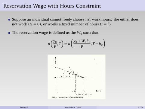
Suppose an individual cannot freely choose her work hours: she either doesnot work (H = 0), or works a fixed number of hours H = h0

The reservation wage is defined as the W0 such that

u�y0

P, T�

= u�

y0 +W0h0

P, T − h0

�


Intensive Margin

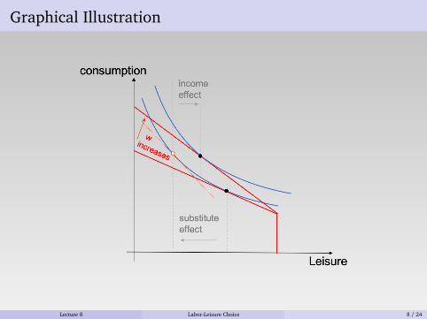
Higher W makes leisure more expensive: substitution effect is negative(choose less leisure)

Higher W increases full income. Assume leisure is a normal good. Thenincome effect is positive (choose more leisure)

Overall effect is ambiguous: labor supply can be upward sloping or backwardbending


Graphical Illustration


Slutsky Equation

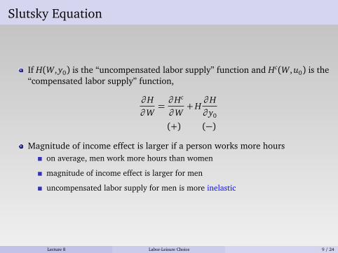
If H(W, y0) is the “uncompensated labor supply” function and Hc(W, u0) is the“compensated labor supply” function,

∂H∂W

=∂Hc

∂W+H

∂H∂ y0

(+) (−)

Magnitude of income effect is larger if a person works more hourson average, men work more hours than women

magnitude of income effect is larger for men

uncompensated labor supply for men is more inelastic


Labor Supply to an Industry or a Firm

If a firm has no monopsony power, labor supply to this firm is infinitely elastic

Labor supply to a specific industry is more elastic than labor supply to theeconomy as a whole (because a higher wage in one particular industry notonly attracts people to work more intensively, but it attract people working inother industries to move to this particular industry)


Intertemporal Substitution

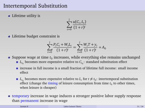
Lifetime utility ist∑

t=0

u(Ct, Lt)(1+ r)t

Lifetime budget constraint is

t∑

t=0

PtCt +WtLt

(1+ r)t=

t∑

t=0

WtT + yt

(1+ r)t+ A0

Suppose wage at time t0 increases, while everything else remains unchangedLt0 becomes more expensive relative to Ct0 : standard substitution effect

increase in full income is a small fraction of lifetime full income: small incomeeffect

Lt0 becomes more expensive relative to Lt for t 6= t0: intertemporal substitutioneffect (change the timing of leisure consumption from time t0 to other times,when leisure is cheaper)

temporary increase in wage induces a stronger positive labor supply responsethan permanent increase in wage


Empirical Findings

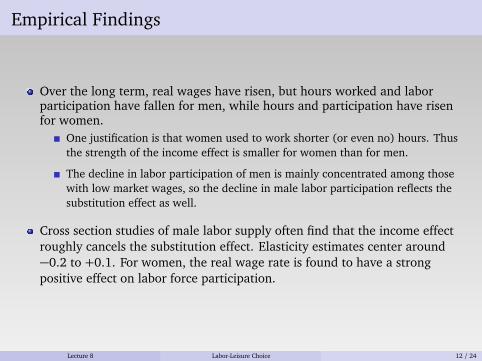
Over the long term, real wages have risen, but hours worked and laborparticipation have fallen for men, while hours and participation have risenfor women.

One justification is that women used to work shorter (or even no) hours. Thusthe strength of the income effect is smaller for women than for men.

The decline in labor participation of men is mainly concentrated among thosewith low market wages, so the decline in male labor participation reflects thesubstitution effect as well.

Cross section studies of male labor supply often find that the income effectroughly cancels the substitution effect. Elasticity estimates center around−0.2 to +0.1. For women, the real wage rate is found to have a strongpositive effect on labor force participation.


Is Leisure a Normal Good?

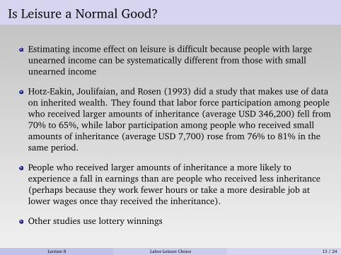
Estimating income effect on leisure is difficult because people with largeunearned income can be systematically different from those with smallunearned income

Hotz-Eakin, Joulifaian, and Rosen (1993) did a study that makes use of dataon inherited wealth. They found that labor force participation among peoplewho received larger amounts of inheritance (average USD 346,200) fell from70% to 65%, while labor participation among people who received smallamounts of inheritance (average USD 7,700) rose from 76% to 81% in thesame period.

People who received larger amounts of inheritance a more likely toexperience a fall in earnings than are people who received less inheritance(perhaps because they work fewer hours or take a more desirable job atlower wages once thay received the inheritance).

Other studies use lottery winnings


Intertemporal Labor Supply

Camerer, Babcock and Loewenstein (1997) finds that New York City taxidrivers work fewer hours on days when the effective hourly wage is high.They propose a “target income hypothesis.”

Gerald Oettinger (1999) studied labor supply of food vendors at a baseballstadium. These vendors are hired on a daily basis and they are free to choosewhether to work at any given game. Earnings from sales fluctuate by thegame, but these fluctuations are to some extent predictable. Thesefluctuations tend to cancel out so the income effect is probably not verystrong (more precisely, one may think of the labor supply response as aresponse to intertemporal wage changes). Oettinger found that a US$10 risein daily earnings (the average was about $43) lured an extra 6 vendors (theaverage number was about 45) to the stadium.


Uber Drivers

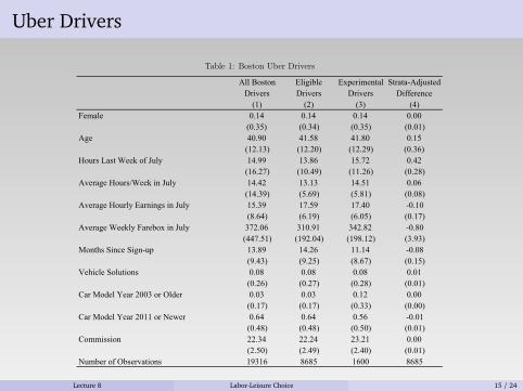
Table 1: Boston Uber Drivers

All Boston Eligible ExperimentalDrivers Drivers Drivers

(1) (2) (3)Female 0.14 0.14 0.14 0.00

(0.35) (0.34) (0.35) (0.01)Age 40.90 41.58 41.80 0.15

(12.13) (12.20) (12.29) (0.36)Hours Last Week of July 14.99 13.86 15.72 0.42

(16.27) (10.49) (11.26) (0.28)Average Hours/Week in July 14.42 13.13 14.51 0.06

(14.39) (5.69) (5.81) (0.08)Average Hourly Earnings in July 15.39 17.59 17.40 -0.10

(8.64) (6.19) (6.05) (0.17)Average Weekly Farebox in July 372.06 310.91 342.82 -0.80

(447.51) (192.04) (198.12) (3.93)Months Since Sign-up 13.89 14.26 11.14 -0.08

(9.43) (9.25) (8.67) (0.15)Vehicle Solutions 0.08 0.08 0.08 0.01

(0.26) (0.27) (0.28) (0.01)Car Model Year 2003 or Older 0.03 0.03 0.12 0.00

(0.17) (0.17) (0.33) (0.00)Car Model Year 2011 or Newer 0.64 0.64 0.56 -0.01

(0.48) (0.48) (0.50) (0.01)Commission 22.34 22.24 23.21 0.00

(2.50) (2.49) (2.40) (0.01)Number of Observations 19316 8685 1600 8685

Strata-AdjustedDifference

(4)

Note: Columns 1-2 compare Boston drivers to the subset of drivers eligible for the experiment. Eligible drivers are those with validvehicle year information who made at least 4 trips during the past 30 days and drove an average of between 5 and 25 hours/week in July2016. Column 3 shows means for treated drivers. Treatment was randomly assigned within strata defined by hours (high/low), commission(20/25% commission) and car age (older/newer than 2003). Column 4 shows the strata-adjusted difference between the treated sample andthe eligible pool. Average hourly earnings include surge but are net of fee. Vehicle solutions drivers lease a car through an Uber-sponsoredleasing program.

33


Field Experiment

Angrist, Caldwell and Hall (2019) did an experiment to create wagevariations for Uber drivers and measure their labor supply response.

1600 drivers were randomly drawn and given the opportunity to drivefee-free in the “opt-in week.” If the Uber fee is 20%, drivers would bereceiving 1 dollar instead of 80 cents per dollar revenue. This represents a25% increase in their hourly wage.

Only 1,031 drivers accepted this opportunity. For those who accepted, theywere offered a further opportunity to participate in two “taxi-weeks.” Theycould continue to drive fee-free if they buy a “lease” for $110 per week.(They can break even if they get $550 revenue that week.)


Effects on Labor Supply

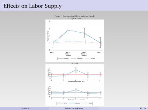
Figure 7: Participation Effects on Labor SupplyA. Opt-in Week

-.20

.2.4

.6Tr

eatm

ent E

ffect

Aug 22 Aug 29Wave 1Treated

Sept 5Wave 2Treated

Sept 11

Hours Farebox Active

B. Taxi

-.4-.2

0.2

.4.6

Trea

tmen

t Effe

ct

-2 -1 0 1 2Relative to treatment week; Taxi 1

-.4-.2

0.2

.4.6

Trea

tmen

t Effe

ct

-2 -1 0 1 2Relative to treatment week; Taxi 2

Hours Farebox Active

Note: These figures report treatment effects on hours, earnings and an indicator of any Uberactivity for drivers who opted in to the Earnings Accelerator. Panel A reports estimates for driverswho accepted the opportunity to drive fee-free. Panel B reports estimates for drivers who bought aTaxi lease. Effects are computed by instrumenting experimental participation with experimentaloffers as described in the text.

47


Instrumental Variables Estimation

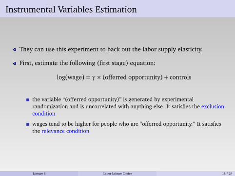
They can use this experiment to back out the labor supply elasticity.

First, estimate the following (first stage) equation:

log(wage) = γ× (offerred opportunity)+ controls

the variable “(offerred opportunity)” is generated by experimentalrandomization and is uncorrelated with anything else. It satisfies the exclusioncondition

wages tend to be higher for people who are “offerred opportunity.” It satisfiesthe relevance condition


Second Stage

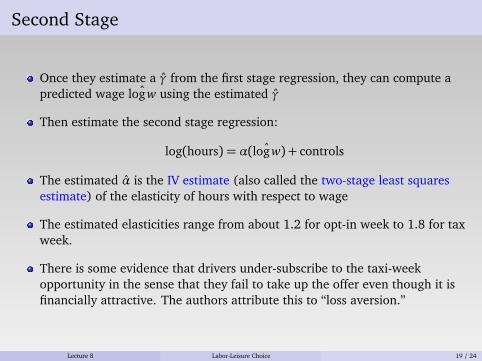
Once they estimate a γ̂ from the first stage regression, they can compute apredicted wage ˆlog w using the estimated γ̂

Then estimate the second stage regression:

log(hours) = α( ˆlog w) + controls

The estimated α̂ is the IV estimate (also called the two-stage least squaresestimate) of the elasticity of hours with respect to wage

The estimated elasticities range from about 1.2 for opt-in week to 1.8 for taxweek.

There is some evidence that drivers under-subscribe to the taxi-weekopportunity in the sense that they fail to take up the offer even though it isfinancially attractive. The authors attribute this to “loss aversion.”


Children and Female Labor Supply

Comparing the labor supply of women with more children against those withfewer children is not enough for causal inference. Why?


Challenge

The challenge is to find an instrumental variable thataffects the number of children (relevance condition)

but is otherwise unrelated to women’s labor supply decision (exclusioncondition)

Angrist and Evans (1998) finds an ingenious IV: the sex parity of children


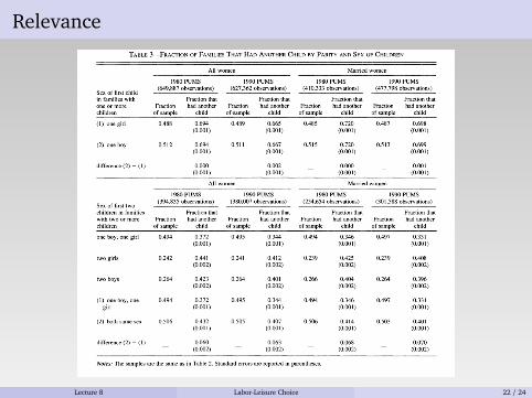
RelevanceVOL. 88 NO. 3 ANGRIST AND EVANS: CHILDREN AND THEIR PARENTS' LABOR SUPP:LY 457

TABLE 3-FRACTION OF FAMILIES THAT HAD ANOTHER CHILD BY PARITY AND SEX OF CHILDREN

All women Married women

1980 PUMS 1990 PUMS 1980 PUMS 1990 PUMS Sex of first child (649,887 observations) (627,362 observations) (410,333 observations) (477,798 observations) in families with Fraction that Fraction that Fraction that Fraction that one or more Fraction had another Fraction had another Fraction had another Fraction had another children of sample child of sample child of sample child of sample child

(1) one girl 0.488 0.694 0.489 0.665 0.485 0.720 0.487 0.698 (0.001) (0.001) (0.001) (0.001)

(2) one boy 0.512 0.694 0.511 0.667 0.515 0.720 0.513 0.699 (0.001) (0.001) (0.001) (0.001)

difference (2) - (1) 0.000 0.002 0.000 0.001 (0.001) (0.001) (0.001) (0.001)

All women Married women

1980 PUMS 1990 PUMS 1980 PUMS 1990 PUMS Sex of first two (394,835 observations) (380,007 observations) (254,654 observations) (301,588 observations) children in families Fraction that Fraction that Fraction that Fraction that with two or more Fraction had another Fraction had another Fraction had another Fraction had another children of sample child of sample child of sample child of sample child

one boy, one girl 0.494 0.372 0.495 0.344 0.494 0.346 0.497 0.331 (0.001) (0.001) (0.001) (0.001)

two girls 0.242 0.441 0.241 0.412 0.239 0.425 0.239 0.408 (0.002) (0.002) (0.002) (0.002)

two boys 0.264 0.423 0.264 0.401 0.266 0.404 0.264 0.396 (0.002) (0.002) (0.002) (0.002)

(1) one boy, one 0.494 0.372 0.495 0.344 0.494 0.346 0.497 0.331 girl (0.001) (0.001) (0.001) (0.001)

(2) both same sex 0.506 0.432 0.505 0.407 0.506 0.414 0.503 0.401 (0.001) (0.001) (0.001) (0.001)

difference (2) - (1) _ 0.060 0.063 0.068 0.070 (0.002) (0.002) (0.002) (0.002)

Notes: The samples are the same as in Table 2. Standard errors are reported in parentheses.

section show the sample characteristics of women in the following groups: those with one boy and one girl, those with two girls, and those with two boys. The next two rows report estimates for women with two children of the same sex and for women with one boy and one girl. The final row reports the differences between the same-sex and mixed-sex group averages.

Both data sets and samples suggest that women with two children of the same sex are much more likely to have a third child than the mothers of one boy and one girl. For example, in the 1980 all-women sample, only 37.2 percent of women with one boy and one girl have

a third child, compared to 43.2 for women with two girls or two boys. The relationship between sex mix and the probability of additional childbearing is even larger for married women, reaching a precisely estimated 7- percentage-point difference in the 1990 Cen- sus. This is approximately 21 percent of the rate of additional childbearing among women with one boy and one girl.. Finally, we note that the relationship between sex mix and childbearing is confirmed in data from the fertility supplements to the June 1980, 1985, and 1990 CPS. This is important because, unlike the Census where information about children is partly based on our household match, the


Wald Estimate

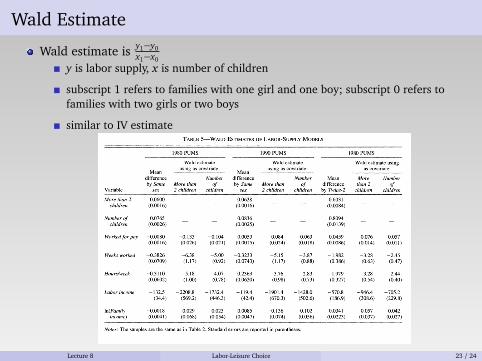
Wald estimate is y1−y0x1−x0

y is labor supply, x is number of children

subscript 1 refers to families with one girl and one boy; subscript 0 refers tofamilies with two girls or two boys

similar to IV estimate460 THE AMERICAN ECONOMIC REVIEW JUNE 1998

TABLE 5-WALD ESTIMATES OF LABOR-SUPPLY MODELS

1980 PUMS 1990 PUMS 1980 PUMS

Wald estimate Wald estimate Wald estimate using using as covariate: using as covariate: as covariate: Mean Mean

difference Number difference Number Mean More Number by Same More than of by Same More than of difference than 2 of

Variable sex 2 children children sex 2 children children by Twins-2 children children

More than 2 0.0600 0.0628 0.6031 children (0.0016) (0.0016) (0.0084)

Number of 0.0765 0.0836 0.8094 children (0.0026) (0.0025) (0.0139)

Worked for pay -0.0080 -0.133 -0.104 -0.0053 -0.084 -0.063 -0.0459 -0.076 -0.057 (0.0016) (0.026) (0.021) (0.0015) (0.024) (0.018) (0.0086) (0.014) (0.011)

Weeks worked -0.3826 -6.38 -5.00 -0.3233 -5.15 -3.87 -1.982 -3.28 --2.45 (0.0709) (1.17) (0.92) (0.0743) (1.17) (0.88) (0.386) (0.63) (0.47)

Hours/week -0.3110 -5.18 -4.07 -0.2363 -3.76 -2.83 -1.979 -3.28 -2.44 (0.0602) (1.00) (0.78) (0.0620) (0.98) (0.73) (0.327) (0.54) (0.40)

Labor income -132.5 -2208.8 -1732.4 --119.4 -1901.4 -1428.0 -570.8 -946.4 -705.2 (34.4) (569.2) (446.3) (42.4) (670.3) (502.6) (186.9) (308.6) (229.8)

ln(Family -0.0018 -0.029 -0.023 -0.0085 -0.136 -0.102 -0.0341 -0.057 -0.042 income) (0.0041) (0.068) (0.054) (0.0047) (0.074) (0.056) (0.0223) (0.037) (0.027)

Notes: The samples are the same as in Table 2. Standard errors are reported in parentheses.

mainder of the paper because this emphasizes the fact that the fertility increment induced by either instrument is a move from two to more than two children.

B. Two-Stage Least-Squares Estimation

While the Wald estimates provide a simple illustration of how the instruments identify the effect of children on labor supply, the rest of the paper discusses two-stage least-squares (2SLS) and ordinary least-squares (OLS) estimates of regression models relating labor- market outcomes to fertility and a variety of exogenous covariates. 2SLS estimation allows us to accomplish three things. First, even if there is no association between the instrument and exogenous covariates, as suggested by Ta- ble 4, controlling for exogenous covariates can lead to more precise estimates if the treatment effects are roughly constant across groups.

Second, we can use 2SLS to control for any secular additive effects of child sex when using Same sex as an instrument. This is desirable because Same sex is an interaction term

involving the sex of the first two children, and therefore potentially correlated with the sex of either child. To see this, let s1 and S2 be indi- cators for male firstborn and second-born children. The instrument can be written as

(3) Same sex =S1S2 + (1 - si)(l - S2)

Assuming that child sex is independent and identically distributed (i.i.d.) over children, the population regression of Same sex on either sj produces a slope coefficient equal to 2E[sj] - 1, which is zero only if E[sj] = 1/2.1

Since the probability of giving birth to a male child is 0.51, there is a slight positive association between Same sex and the sex of each child. This correlation is a concern only if sj

10 Proof: Assuming child sex is i.i.d., we have E[si ] =

E[S2] and E[s1s2] = E [j]2 . Therefore, Cov(Same sex, sj) = E[sj](E[sj] - E[Same sex]). Some manipulation gives E[sj] - E[Same sex] = (1 - E[sj])(2E[sj] - 1). Since the variance of sj is E [sj] (l -E[sj] ), the regression coefficient is (2E [sj] - 1).


Lessons for Causal Inference

Conduct field experiments to manipulate variations in independent variable

Find instrumental variables that satisfy relevance condition and exclusioncondition to get at causal inference


Documents

Labor-Leisure Choice