Labor Productivity:

Structural Change and Cyclical Dynamics

Martin Neil Baily*, Eric J. Bartelsman””, and John Haltiwanger***

January 1996

First Draft: January 1995

Abstract

A longstanding puzzle of empirical economics is that average labor productivity declinesduring recessions and increases during booms. This paper provides a framework to assess theempirical importance of competing hypotheses for explaining the observed procyclicality. Foreach competing hypothesis we derive the implications for cyclical productivity conditional onexpectations of future demand and supply conditions. The novelty of the paper is that weexploit the tremendous heterogeneity in long-run structural changes across individual plants toidentify the short-run sources of pro cyclical productivity y. Our findings favor an adj ustrnent costmodel which involves a productivity penalty for downsizing as the largest source of procyclicallabor productivity.

‘University of Maryland and NBER; **Federal Reserve Board; ***University of Maryland and NBER; ResearchAssociate and CES Fellow, Census Bureau.The views expressed herein are solely the authors’. We wish to thank the stfi and visiting researchers at the Centerfor Economic Studies, U.S. Bureau of the Census, for providing a stimulating reseaxch environment. We would alsolike to thank participants of the NBER Summer ’93 workshop, the 1995 NBER Small Group Meeting on AlternativeExplanations of Employment Fluctuations, the 1995 SITE workshop, the Econometric Society meetings, January1995, and seminar participants at several universities and institutions for valuable comments and suggestions.

1 Introduction

A longstanding puzzle of empirical economics is that average labor productivity declines during

recessions and increases during booms. There is no shortage of possible explanations for the pro-

cyclicalit y and no shortage of studies attempting to identify the source of the procyclicalit y. 1 Tra-

ditionally, these explanations have fallen into two categories: the underlying theoretical framework

was adjusted, by assuming market imperfections or non-standard production technology, or the

data were adjusted for assumed measurement error in either output or labor. Despite these pos-

sible adjustments, there is no consensus as to which explanation is the predominant cause of the

procyclicalit y. (he important reason for this is that most research on this issue uses aggregate or

sect oral level data and has difficult y distinguishing underlying causes because they have observa-

tionally equivalent implications for these data. 2 The novelty of this paper is that we exploit the

tremendous heterogeneity in long-run structural changes across individual plants to identify the

sources of short-run procyclical productivity.

We analyze a balanced panel of data on output, employment and hours for all large continuously

operating plants in U.S. manufacturing from 1972 through 1988. We use the cross sectional variation

in the long-run structural changes of supply and demand conditions to distinguish causes of cyclical

movements in plant level productivity. For example, during recessions it is plants that expect desired

employment to recover that should hoard labor. Accordingly, if labor hoarding is the prime cause

of procyclical productivity, one would expect to find more cyclical variation in productivity for

those plants that expected to expand (or at least not contract) their labor force in the long run.

The main points of this paper would have been well known to macroeconomists if appropriate e

aggregations or decompositions of the data had been available at an earlier stage. For example,

the decomposition of employment changes into gross flow categories—job creation and destruction

-made by Davis and Halt iwanger (1990) has allowed new insights into labor market mechanisms

and lxlsiness cycle determinants. Likewise, we think that a decomposition of data on production

and prodllct ive hqmts into categories based on the underlying agents’ long-run changes (Le., de-

composing on the basis oft he long run micro change being positive or negative) provides important

information on short-run movements.

We distinguish between five possible sources of procyclical labor productivity: labor hoard-

ing, adjust ment costs, external economies, increasing ret urns to scale and compositional changes.

The first folu- are the purview of traditional macroeconomics, while the last is associated with re-

lThis is a long literature with antecedents in the Dunlop/Tarshk/Keynes debate about the behavior of real wagesover the business cycle. Notable contributions to this literature across the clecades include Kuh (1965), Fair (1969),Solow (1973), Fay and Medoff (1985), Hall (1988) and (1990), Gordon (1990), Bernanke and Parkinson (1991),Burnside, Eichenbaum, and Rebelo (1993).

2A notable exception is Aizcorbe (1992), who analyses cyclical labor productivity in automobile assertiiy plants.In auto assenhlies labor hoarding turns out to prevalent, likely owing to the specific nature of labor contracts in thatindustry.

1

cent research on the importance of heterogeneity and cross-sectional dynamics for understanding

aggregate fluctuations.

One potential problem in using the long-run structural changes to identify the sources of short-

run procyclical productivity is that the latter may influence the former. To correct for possible

endogeneit y of long-run changes, we also conduct our analysis using estimates of plant level fore-

casts, rat her than ex-post realizations, of structural change in demand and supply. This approach

is possible because we have time series data starting in 1972, but only consider the cyclical episodes

post 1979. Using such forecasts not only addresses the potential endogeneity problems but is con-

sistent with the underlying theory in which the response of an individual producer to an adverse

cyclical shock depends on expectations of future demand and cost conditions.

The organization of our paper is as follows: First we give a description of the various hypotheses

of sources of procyclical labor productivity and relate these to the existing literature. Next, we

describe our sample of plants, and compute the size of the mix shift effects. Following this, we

present a model that ties sources of procyclicality to long-run changes, and describe the testable

implications for the data. In the empirical section we investigate the cyclical behavior of labor

productivity for sub-samples of our data, split according to the long-run changes in plant level

employment and product ivit y. We also describe our econometric methodology and present our

results. We conclude with a summary and ruminations about extensions to this research.

2 Possible Explanations for Procyclical Productivity

The first hypothesis is that there are increasing returns to scale at the plant level: Increases in

inputs of a given percentage result in increases in output of a larger percentage due to increasing

ret urns in plant level production functions. The declines in output that characterize recessions

will then naturally lead to declines in total factor productivity, and, depending on the specific

parameters of the production function and on the extent of lumpiness in capital use, a decline

in labor productivity. If increasing returns is the main explanation for the cyclical productivity

puzzle, we also expect to see evidence of increasing returns in the long-run behavior of Plants and

in the parameters of the long-run production function.

The second hypothesis is that plants hoard labor over the cycle. We define labor hoarding in

a very specific way, one that is linked to the work of Oi (1962). It is argued that firms create

firm-specific human capital in their employees. When output levels fall, there are workers that are

not needed for current production, but that are retained on the payroll by the firm in order to

preserve their human capital.

A key element of this labor hoarding model is that firms must believe that output and labor

demand will recover in some future period. It is not worth keeping excess workers on the payroll

that will not be used in the future. Under uncertainty, this means that the optimal amount of labor

2

hoarding will be smaller the lower is expected future employment.

Closely related to the labor hoarding hypothesis is the mismeasurement hypothesis proposecl

by Gordon (1990), Saint-Paul (1993) or Bean (1990), Gordon argues that workers are assigned

to maintenance or other tasks during periods of low production. It is natural to suggest that

workers held for human capital reasons would be assigned to maintenance tasks. The true output

of the firm is higher than the measured output in recessions, because the value oft he maintenance

tasks is missed. Bean takes this a step further, and argues that during recessions workers build

up their human capital by supplying labor to an unmeasured human capital production function.

The increased skills learned during the recession can then be employed during the recovery to give

an extra productivity impulse. The mismeasurement hypothesis carries the same implications as

the labor hoarding hypothesis. The opt imal number of workers assigned to maintenance or human

capital accumulation will be smaller the lower is expected future employment.

The third hypothesis is that there is a contemporaneous productivity penalty induced by chang-

ing the scale of operations. For example, when output declines, it is difficult to rearrange the pro-

duction process so as to maintain productivity. Over time, if the lower level of output is sustained,

productivity can recover (and perhaps ultimately increase) as the production process is adjusted.3

Consider plants that face such a productivity penalty from adjusting the scale of operations.4

For plants that are also on a long-run path of employment decline, a temporary downward shock

will accelerate the ongoing downsizing which in turn will exacerbate the adjustment cost penalty to

productivity. A sufficiently large productivity penalty from downsizing can account for procyclical

productivity for such plants. In contrast, plants that expect employment to increase in the long-

run will reduce employment less in response to the same temporary downward shock. Thus, in the

case of an adjustment-cost-induced productivity penalty, procyclical productivity should be most

evident among long-run downsizing plants. This is in cent rast to the labor hoarding case.

The fourth hypothesis is that there are externalities. Productivity is higher when all plants

increase output together and productivity falls when the output of most plants falls. AI1 implication

‘] The adjustment costs that we emphasize are those that generate productivity penalties associated with changesin the scale of operations. In the terminology of the adjustment cost literature (see, e.g., Brechling (1975)), ourspecification is one of internal adjustment costs. This contrasts with the predominant recent treatment of employ-ment adjustment costs in the literature (see, e.g., Sargent (1978) and Hamermesh and Pfann (1994)) that formallycharacterize the adjustment costs as external adjustment costs. In our view, it is somewhat puzzling that the assump-tion of external adjustment costs has become the standard in the literature. A common motivation for employmentadjustment costs is the presence of hiring and training costs. A related second motivation is that changing the sizeof the workforce can be disruptive in terms of the coordination and teamwork across workers. Both of these ideasbetter motivate internal rather than external adjustment costs. Of course, some hk-ing and training costs arguablydo not directly tiect productivity but rather reflect explicit costs. For example, some union agreements specifyseverance payments or other penalties for employment reductions. This chstinction between internal and externaladjust ment costs is of fundamental importance in this cent ext. While internal and external adjustment costs havesimilar implications with respect to employment dynamics, they have potentially very WYerent implications withrespect to productivity dynamics.

4The focus of the intuitive discussion involves aproductivity penalty for upsizing would contribute

productivity penalty for downsizing. As discussed in section 4, ato countercyclicality rather than procyclicality of labor.

3

of this hypothesis is that the productivity impact of a demand or technology shock in a given

plant should depend upon whether this decline is idiosyncratic to the plant or whether it occurs

simultaneously in most manufacturing plants. Bart elsInan et al, (1994) have found evidence for a

modest posit ive relationship between downstream activity and productivity over the course of a

business cycle.5

Lastly, we look at the effect of mix-shifts or industry composition on the measured procyclicality

of aggregate labor productivity y in manufacturing. Recent work investigating plant and firm level

dynamics of productivity has shown the importance of distinguishing ‘within’ plant productivity

growth and the effects of compositional change on the aggregate. Bartelsman and Dhrymes (1994)

show that in a sample of large manufacturing plants, long-run total factor productivity (TFP)

growth is mostly the results of compositional changes: on average, plant level productivity y does not

increase over time, while, on balance, more productive plants become larger while less productive

plants lose market share. A similar finding is reported in Baily, Hulten and Campbell (1992),

who investigate all plants in a subset of 4-digit industries. By contrast, Baily, BartelSInaIl and

Haltiwanger (1995) and Griliches and Regev (1992) find that for long-run labor productivity, most

of the aggregate growth is the result of within plant growth.

While it is beyond the scope of this paper to reconcile these differing results on total factor

productivity and labor productivity, the above mentioned research does suggest the possibility that

the aggregate pattern of procyclical labor productivity may arise from a mix-shift effect.6 Perhaps,

most plants display the neoclassical pattern of countercyclical productivity, but the aggregate data

are ‘distorted’ by the mix changes. For this hypothesis to be correct, it would mean that below

average productivity plaints have larger shares of employment in recessions than they have in booms,

or that the net effect of entry and exit on productivity has a clear procyclical pattern.7

3 Data Description and Exploration

3 . 1 D a t a D e s c r i p t i o n

In this study we make use of a sample of manufacturing plants from the Longitudinal Research

Database (LRD), available at the Bureau of the Census. our sample consists of those plants which

were in continuous operation from 1972 through 1988, and had positive employment and shipments

SID *IlanY ~aYS, the current ~aPer can be interpreted as exploiting within sector, between Plant dmerences ‘n ‘he

sectoral level results found in Bartelsrnan et al. (1994).6Similar decompositions have been made for the cyclical variation in real wages - See the recent survey by Abraham

and Halt iwanger (1995). The consensus that emerges from these st uclies is that there is a counter cyclical compositionbias in real wages induced by the fact that lower skilled workers tend to be laid off first in recessions. After correctingfor this composition bias, researchers have typically found that wages are procyclical.

‘In our investigation we use a balanced panel of plants and cannot check the net effect of entry and exit directly.We do not think that this effect is disproportionate, in any case, since the cyclical pattern of productivity in oursample is similar to that of the aggregate. In fact, the subsequent discussion of Chart 1 suggests that if anything netentry yields a countercyclical contribution to productivity over the cycle.

4

in all years. Given the nature of the Annual Surveys of Manufactures, this selection criterion

provides us with a sample of firms which are much larger than average. Table 1 provides summary

stat istics of olm sample, compared with all manufacturing for 1987. As shown, we cover less than

2-1/2 percent of plants, but nearly half of the output in manufacturing.

Chart 1 provides a comparison of our LRD sample with data for all manufacturing. The

top panel shows output and employment for all manufacturing, the middle panel displays the same

series for our LRD sample, while the bottom panel compares output per hour from our sample with

that from all manufacturing. Output is measured as deflated shipments plus inventory changes,

using 4-digit benchmark- years weighted out put deflators. 8 Employment is measured in hours, and

k constructed as the sum of production worker hours and non-production workers multiplied by

the average length of their workweek. Annual time series on the workweek for non-production

workers is computed for 2- and some 3-digit industry groupings using information from the Current

Population Survey. In later analysis, we also look at variants of employment and productivity, with

out put measured by double-deflated value added, and employment measured by total number of

employees.

The central point of Chart 1 is that the basic aggregate properties of output, employment,

and productivity fluctuations for our sample are the same as those exhibited by the published

series. Specifically, for our sample and the published series, out put and tot al hours are procyclical,

out put is more cyclically volatile than total hours and, accordingly, average labor productivity is

procyclical. There are some quantitative differences in the nature of the cyclicality between our

sample and the published series that we explore below.

3.2 The Contribution of Simple Composition Effects

We now turn to the last hypothesis for procyclical productivity, that of composition effects. As

stat ed earlier, we are not able to discuss the effect of plant turnover on productivity movements

directly. As seen in the bottom panel of chart 1, however, our sample appears to have more cyclical

productivity than the aggregate for all manufacturing. This would agree with our prior belief that

less productive plants are more likely to exit in a trough, and reduce the procyclicality of the

aggregate.

For our sample of cent inuing plants, we can decompose annual productivity changes into a

‘within’ plant component, and two mix-shift terms: an employment share effect, and a cross term.

Ant _ D 4t-I,ifWi + xi Ag5@_l,i + ~z A&;AII~,iH~_l rI_ 1 rI_l rI_l ‘

(1)

‘The deflators and data for total manufacturing are computed from the 4-digit NBER Manufacturing ProductivityDatabase, available via anonymous FTP from nber.harvard.edu. See Bartelsman and Gray (1995) for a descriptionof these data.

5

Table 1: 1987 Summary Statistics: All Mfg. vs. LRD %rnple

All Mfg. LRD Sample Sample m % of AllEstablishments 368897 8669 2.34

Output (Billions)Employment (000)Avg. Estab. Size

2329.6 1100.7 47.25

17406.5 6332.8 36.3847 731

Plant DistributionBy SIC20212223242526272829303132333435363738

20583137

6065231683398711636

62926179112039

223214589

219816191

66613609252091159221050510193

89122

608519180247430431537103332143299506721859918505276

4.3316.0610.022.240.532.126.836.984.464.612.286.511.857.602.001.655.764.812.71

39* Excludes computers> SIC 3573.

16573 142 0.86

where IIi is output per hour in plant i, Lz shows employee hours in plant i, and & = -&L, ‘Chart 2 shows the time series behavior of the three components over our sample period. The

productivity (within plant) term exhibits pronounced procyclical behavior, with sharp increases

in the recovery years 1976 and 1983. The first mix term (employment share) rises because of

shifts in employment shares between plants, This term k positive or negat he depending upon

whether the plants that are above average in productivity are increasing or decreasing their shares

of employment. There was a substantial employment effect that increased productivity in 1981,

82, and 83. Cyclical episodes thus tend to shake the plants up in the “right” direction, that k, it

raised the employment share of above average plants.

The cross-term was negative in the early 1980s, indicating that plants that increased produc-

tivity more rapidly than average had dediIlillg employment shares – consistent with the fact that

some plants were more successful than others in adjusting their employment over the period. On

balance, however, this term is quite small.

3.3 Bas ic Fac t s : Long- run S t ruc tu ra l Change and Cyclical D y n a m i c s

Although there are non-trivial mix effects shown in these data, it seems that a fair general charac-

terization of the results is that procyclical productivity is a within-plant phenomenon. Even though

the cyclical variation in productivity is primarily due to within-plant effects, this does not imply

that there are no cross sectional differences across plants that are in important in accounting for the

procyclicality of productivity. For example, Baily, Bartelsrnan and Hahiwanger (1995) have shown

that there are import ant cross sect ional differences across plants that are important in accounting

for the secular growth in productivity in the U.S. manufacturing sector in the 1980s. Surprisingly,

plants that upsized (increased employment) and increased productivity accounted for about ass

much of the increase in overall productivity as plants that downsized and increased productivity.

Over the 1980s, upsizing plants that increased productivity saw their share of manufacturing output

increase from about 20’%0 to 40% which is one of the primary reasons that aggregate productivity

increased over this period.

The long-run differences between upsizing plants and downsizing plants potentially have im-

portant implications for short-run cyclical changes ass well. As discussed in section 2, cyclical

productivity fluctuations are naturally linked to long-run structural changes. The evidence of

subst ant ial heterogeneity y in the long-run structural changes found by Baily, Bart ekman and Halt i

wanger (1995) thus provides a source of variation in the data that can be exploited to identify the

relative cent ribution of alternative explanations of pro cyclical productivity y.

To begin this exploration of the connection between the cyclical variations in productivity and

the long-run structural changes, we consider the cyclical productivity fluctuations of plants for

each of four quadrants: plants where employment and productivity increased in the long run,

plants where productivity increased and employment declined, plants where employment and pro-

7

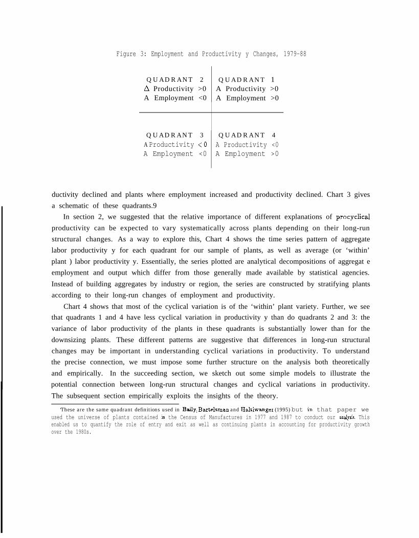
Figure 3: Employment and Productivity y Changes, 1979-88

QUADRANT 2 QUADRANT 1A Productivity >0 A Productivity >0A Employment <0 A Employment >0

QUADRANT 3 QUADRANT 4A Productivity <0 A Productivity <0A Employment <0 A Employment >0

ductivity declined and plants where employment increased and productivity declined. Chart 3 gives

a schematic of these quadrants.9

In section 2, we suggested that the relative importance of different explanations of procyclical

productivity can be expected to vary systematically across plants depending on their long-run

structural changes. As a way to explore this, Chart 4 shows the time series pattern of aggregate

labor productivity y for each quadrant for our sample of plants, as well as average (or ‘within’

plant ) labor productivity y. Essentially, the series plotted are analytical decompositions of aggregat e

employment and output which differ from those generally made available by statistical agencies.

Instead of building aggregates by industry or region, the series are constructed by stratifying plants

according to their long-run changes of employment and productivity.

Chart 4 shows that most of the cyclical variation is of the ‘within’ plant variety. Further, we see

that quadrants 1 and 4 have less cyclical variation in productivity y than do quadrants 2 and 3: the

variance of labor productivity of the plants in these quadrants is substantially lower than for the

downsizing plants. These different patterns are suggestive that differences in long-run structural

changes may be important in understanding cyclical variations in productivity. To understand

the precise connection, we must impose some further structure on the analysis both theoretically

and empirically. In the succeeding section, we sketch out some simple models to illustrate the

potential connection between long-run structural changes and cyclical variations in productivity.

The subsequent section empirically exploits the insights of the theory.

‘These are the same quadrant definitions used in Baily, Bartelsman and Haltiwanger (1995) but h that paper weused the universe of plants contained in the Census of Manufactures in 1977 and 1987 to conduct our analysk. Thisenabled us to quantify the role of entry and exit as well as continuing plants in accounting for productivity growthover the 1980s.

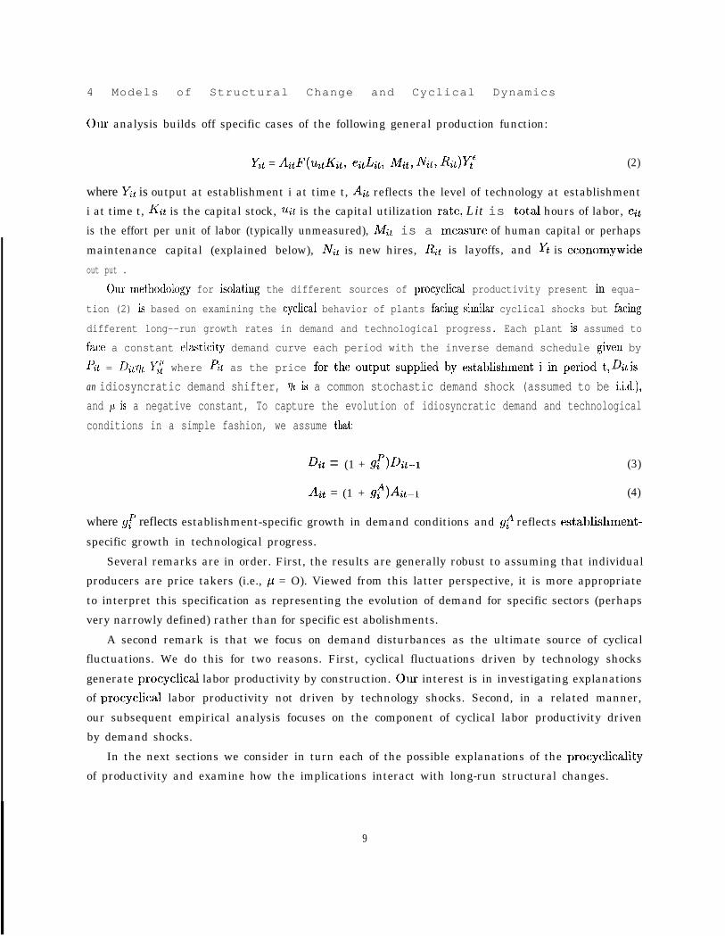
4 Models of Structural Change and Cyclical Dynamics

(hr analysis builds off specific cases of the following general production function:

Yit = AitF(wKit, eith, J&, Nit, Rt)yf (2)

where Yit is output at establishment i at time t, Ait reflects the level of technology at establishment

i at time t, Kit is the capital stock, uit is the capital utilization rate, Lit is total hours of labor, eit

is the effort per unit of labor (typically unmeasured), M2t is a measure of human capital or perhaps

maintenance capital (explained below), IV;t is new hires, R~t is layoffs, and Yt is economywide

out put .

our methodology for isolating the different sources of procyclical productivity present in equa-

tion (2) is based on examining the cyclical behavior of plants facing similar cyclical shocks but facing

different long--run growth rates in demand and technological progress. Each plant is assumed to

face a constant elasticity demand curve each period with the inverse demand schedule given by

F’it = ~itqt Yz~ where f’~t as the price for the output supplied by establishment i in period t, Qt is

an idiosyncratic demand shifter, qt k a common stochastic demand shock (assumed to be i.i.d.),

and ~ k a negative constant, To capture the evolution of idiosyncratic demand and technological

conditions in a simple fashion, we assume that:

D~t = (1 + g:pit-1

Ait = (1 + g$)&l

(3)

(4)

where g! reflects establishment-specific growth in demand conditions and g! reflects establishment-

specific growth in technological progress.

Several remarks are in order. First, the results are generally robust to assuming that individual

producers are price takers (i.e., p = O). Viewed from this latter perspective, it is more appropriate

to interpret this specification as representing the evolution of demand for specific sectors (perhaps

very narrowly defined) rather than for specific est abolishments.

A second remark is that we focus on demand disturbances as the ultimate source of cyclical

fluctuations. We do this for two reasons. First, cyclical fluctuations driven by technology shocks

generate procyclical labor productivity by construction. our interest is in investigating explanations

of procyclical labor productivity not driven by technology shocks. Second, in a related manner,

our subsequent empirical analysis focuses on the component of cyclical labor productivity driven

by demand shocks.

In the next sections we consider in turn each of the possible explanations of the procyclicality

of productivity and examine how the implications interact with long-run structural changes.

9

4 . 1 L a b o r H o a r d i n g

The hypothesis of labor hoarding is intimately linked to the appropriate measurement oft he labor

input and to the alternative productive uses of the labor input. The labor input can be thought

of as composed of two components: time spent directly on production, denoted azt, and time

spent on maintenance or training, denoted mit. In terms of the notation in (2), e~t~~t = xit and

z~t + m~t = Lit. To capture the idea that time spent on maintenance or training is ultimately

productive, we define Mit to be human capital or maintenance

Mit+l = (1 – &)Mit + ?nzt

where & is the depreciation rate for this form of capital.

For this specific case, the production function is assumed

capital that accumulates as follows:

(5)

to be given by Y~t = A~tF(~ztj Mit)

where both inputs into the production function have positive marginal products. We omit the

internal adjustment cost terms, externalities and physical capital (for this case) to focus on the

implications of labor hoarding.

The

ment in

value function characterizing the maximization problem faced by an individual establish-

this environment is given by:l”

V(Mit; Dit_l , Ait–l) = ~CZZ (PitAitF(zit, Mit) – ~tLit + ~[Pv(Mit+l ; ~it, Ait)]) (6)

where p is the discount factor, w is the common Wage rate faced by all establishments, and the

evolution of demand and technology conditions are given by equations (3) and (4).11

The maximization problem (6) yields a standard first order condition for employing labor and

an Euler equation for accumulating maintenance/training capital given by:

PitAitF1it = Wt (7)

pitAitF1it = ~E[~it+l Ait+l ((1 – &) Flit+l + F2it+I )] (8)

where pit = (1 + p) nit ~tFi~ and F1 it represents the derivative of the production function iIl tiIne

t with respect to the first argument, and so on. Equation (7) is the standard condition that labor

is employed directly in current production up to the point that the marginal revenue product of

labor is equal to the wage. Equation (8) indicates that labor is utilized in maintenance/training

activity to equate the marginal revenue product of labor in the current period with the expected

discounted future value of an additional unit of maintenance capital.

For our purposes, the main result that emerges from equations (7) and (8) is that ?nit is an

Iowe ~~~unle that the ~aanleters of the pro~uct,ion and demand functions are Such that this is a well-~ehave~

concave nlaximization problem with a unique interior solution.1 L Implicit in the latter is the assumption that the plant faces a constant elasticity demand curve each period.

10

A 12 This result is intuitive since it essentially states that the returnincreasing function of g? and gi .

to engaging in the maintenance/training activity is increasing in the growth rat es of demand and

technological change. Since establishments with more favorable future conditions invest in more

maintenance/t raining capital, this in turn implies that the magnitude of mismeasured labor effort is

great er for establishments with higher long-run growth rates in demand and technological progress.

Further, establishments with more favorable future conditions will exhibit higher long-run growth

of employment – i.e., they will be the upsizers.

Formally, the cyclical responsiveness of average labor productivity is given by:

(k/h)[((%t + Wt)f’lit - ~it)/(w + %t)2] (9)

Equation (9) indicates that incorporating the possibility of maintenance/training capital provides

the potent ial for accounting for procyclical productivity through the mismeasurement of labor

effort. Further, the magnitude of the mismea.surement of labor effort is greater for upsizing plants

which in turn implies that if this is the driving force underlying procyclical productivity then this

effect sholdd be more important for up sizing plants. 13 In terms of our quadrant definitions, this

implies that est abolishments in quadrants 1 and 4 (the long-run upsizers) should be more likely

to exhibit procyclical productivity. This is the key prediction of this model that we test in the

empirical analysis.

4.2 Product ivit y Penalty From Changing Scale of o p e r a t i o n s

We now turn our attention to adjustment costs that involve a disruption in productivity when the

scale of operations is altered. As discussed in section 2, there may be other aspects of adjustment

costs that are import ant in employment d ynarnics that affect the volatility of employment and

outpllt but do not have direct implications for productivity.

For this specific case, we focus on a specification of the production function given by Yz~ =

At~(-ht, Nit, &t ) where Lit = J&I + Nit – Rit. The key assumptions are that the derivatives of

the production function with respect to the second and third arguments are both negative and the

‘2 The details of the results in thk section are derived in Appenchx A.13We thank Dale Mortensen for pointing out to us that the model and implied results become substantially more

complicated when qt exhibits serial correlation. In the latter case, the effect in equation (9) is still present but there isan additional effect involving the response of nt~~ to qt. Since maintenance activity only yields returns in the future,under the i id assumption for the cyclical shock 7n,t is independent of the realization of qt. However, with serialcorrelation, this independence no longer holds. A number of issues are then potentially relevant. First, the nature ofthe serial dependence is relevant – simple first order positive serial correlation would imply procyclical maintenancecapital while a simple Markov switching rule with demand switching between high and low states with probabilityone each period would yield countercyclical maintenance capital. In addition, for our purposes we need to know thesensitivity of the cyclicality of mit to long run conditions. The latter will depend on thkl derivatives that we knowrelatively little about. We emphasize the simpler case with iid shocks because it highlights the interaction of themismeasurement of labor with long run structural changes and it is the rnismeasurement of labor which is at thecenter of the empirical literature on labor hoarding.

11

marginal adjustment cost is increasing (i.e., F22 <0 and F33 < O).’4

A key feature of this specification is t hat the negative second and third derivatives have opposite

effects on the cyclicality of productivity. The productivity penalty associated with hiring will tend

to dampen any forces generating procyclical productivity. In contrast, the productivity penalty

associated with making layoffs will tend to reinforce any forces generating procyclical productivity.

A related important element of this specification is that the productivity disruption associated with

changing the scale of operations can be asymmetric. 15

For this model, the value function characterizing the maximization problem for establishment i

at time t is given by:

V(Lit_l; Dit_l, Ait_l) = rnaz (PitAitF(Lit, Nit, Rit) – wLit + JWv(Lit; ~it, A~~)l) (lo)

The evolution of demand and technology are assumed to be the same as in the previous subsection

(i.e., given by equations (3) and (4)). The Euler equations are given by:

%4 (Flit + &) – &13[~it+1Ait+1F2it+1 IJVit+l > O]

+ /3.E[~it+l Ait+l F3it+I Il?.it+l > O] = wt, if lV~t >0

&Ait (Flit – F3it) – P~[&+lAit+d%t+l Pit+l > 0]

+ /3E[Pit+l Ait+l F3it+l Illit+l > O] = wt, if & >0

(11)

(12)

where Fit = ( 1 + ,U)~it’7]t~~,.

A quick comparison of these two equations imply that new hires and layoffs will not occur

simultaneously. AII est abolishment making layoffs today takes into account both the current and

the expected future adjustment costs in making employment adjustments. The latter in turn

depend on future demand and t ethnology conditions. The impact of expected future adjustment

costs implies that an establishment will reduce employment by a greater amount in response to an

adverse current demand shock (represent ed by a lower }Zt ) the lower is the expected future growth

of demand and technology (represented by a lower ~it+l and Ait+l ) .16 This result in turn implies

that an establishment that anticipates it will be contracting in the future will exhibit a greater

contraction of employment today in response to an adverse demand shock.

In this specification, average labor productivity is given by F(Lit, Nit, &t)/ (Lit-l + Nit – Rit).

When making layoffs (i.e., &t > O) the cyclical responsiveness of average labor productivity is

given by:

‘4 We assume that F(. ) is continuously differentiable.15This asymmetry does not imply the type of non-differentiability of adjustment costs at zero that is emphasized

by Bentolila and Bertola (1992). In fact, our derivation of results assumes continuous differentiability of F(.).16 The details of the derivation of the results in this section are presented in Appendix A.

12

- (mi,/&/,)[((F,,, - F,i,)L,, - Fi,)/(L;,)] (13)

Equation (13) implies that incorporating the possibility of a productivity penalty from downsizing

provides the potential for accounting for procyclical productivity through a productivity penalty

associated with downsizing. Since F33 <0, the greater layoffs by downsizing plants yields a greater

productivity penalty for such plants and thus if this is the driving force underlying procyclical pro-

ductivity then it should be the long-run downsizing plants that exhibit the greatest procyclicality.

ln terms oft he quadrant definitions, the hypothesis is that long-run downsizers (quadrants 2 and

3) make greater layoffs in response to a common adverse cyclical shock which in turn implies that

they will suffer a greater productivity disruption from adjusting the scale of operations downwards.

4.3 Increasing Ret urns – Internal vs. External

Internal increasing returns is characterized by assuming that F(.) exhibits increasing returns with

respect to capital and labor. To illustrate the possible connection between short-run procyclical

productivity and long-run increasing returns, we consider a production function given by Y& =

& (uitKit )QL~ where u~t is the capital utilization rate and a + P > 1. Assume further that

capital is fixed in the short run but that capital utilization is proportional to employment so that

uit = q5Lit . 17 With the same assumptions about the evolution of demand and technology conditions

used in the previous sections (and the same not at ion for marginal revenue), this specification implies

the following standard static first order condition for employment in the short run given by:

&Ait(a + @(@@”L;+o-l = Wt (14)

Equation (14) implies procyclical employment. Given that average labor productivity in this

case is given by Ait (qWit)a L~+$– 1 and a + /3 > 1, this result implies short-run procyclical labor

productivity. Further, by construction long-run changes in output and inputs will also exhibit

increasing returns, Putting these two results together yields the key idea for our purposes: plants

with increasing returns should exhibit behavior consistent with increasing returns in both the short

run and the long run. Establishments with increasing employment and increasing productivity

over the long run (as well as est abolishments that exhibit decreasing employment and decreasing

productivity) should exhibit behavior that is consistent with increasing returns. Accordingly, it

should especially be these establishments (establishments in quadrants 1 and 3 in our classificat ion

of the previous section) that should exhibit procyclical productivity if increasing returns is the

primary source of procyclical productivity. 18

lTThis assumption of proportionality is related to but quite dktinct from that used by Burnskle, Eichenbaurnand Rebelo (1995). The latter paper exploits the assumption that capital utilization is proportional to electricityconsunlpt ion.

18A ~eakne5S of ~h15 ~gumen~ is the &.iving forces underlying long-run Structural changes may induce changes

13

ln contrast, if external increasing returns is the primary source of procyclical productivity then

all establishments should exhibit pro cyclical productivity. 19 In terms of the quadrant definitions,

this prediction implies that there should not be significant differences in the procyclicality across

quadrants.

4.4 Putt ing the Pieces Together

In this section, we have sketched out simple models to show that different sources of procycli-

cal productivity have different implications for establishments with different long-run structural

changes in employment and productivity. The predictions in terms of our quadrant definitions are

sllmmarized briefly as follows. If labor hoarding is the primary source of procyclical productivity,

then quadrants 1 and 4 should exhibit greater procyclicality. If adjustment costs due to downsizing

are the primary source of procyclical productivity, then quadrants 2 and 3 should exhibit greater

procyclicality. If internal increasing returns is the primary source of procyclical productivity, then

quadrants 1 and 3 should exhibit greater procyclicalit y. Finally, if external increasing returns is the

primary source of procyclicality, then it should be observable to the same degree in all quadrants.

5 Empirical I m p l e m e n t a t i o n

Chart 4 provided suggestive evidence that quadrants 2 and 3 exhibit the most procyclicality. How-

ever, the differences in cyclical variation of labor productivity by ex-post quadrants do not suffice

for identifying causes of procyclicality. First, the predictions outlined in section 4 are based on

anticipated structural changes. That is, the predictions are based on anticipated or forecasted

quadrants, not necessarily ex-post quadrants. In a related manner, ex post long-run structural

change may be influenced by the short-run cyclical changes so that allocation into the ex post

quadrants may endogenously interact wit h the short-run cyclical variations in productivity. We

correct for these related problems by making plant level projections of long-run changes, based on

plant specific information prior to 1979.

An additional problem is that sectors may face differences in the magnitude of the cyclical

shocks. This is a problem in this context to the extent that the quadrants have a specific sectoral

composition so that the magnitude of the cyclical episodes vary systematically by quadrant. We

correct for this problem by relating the plant level cyclical variation to a downstream demand

indicator specific to the 4-digit industry to which the plant is assigned.20 An additional advantage

in factor intensities. To the extent that this is important, this approach for identifying the contribution of internalincreasing returns is problematic.

‘gMore precisely, productivity at each imhviclual establishment should be increasing in the relevant measure drivingthe external economies.

‘“The down~treanl indicator is an index of activit,y of other industries and service sectors which purchase outPut

from the industry in question. See Bartelsrnan, Caballero, and Lyons (1994) for a complete description.

14

of using the downstream indicator to capture cyclical fluctuations is that for many industries

(see Shea (1993)) this isolates the component of procyclical productivity associated with demand

fluctuations. As argued by Shea (1993), downstream demand is a better demand instrument when

the materials share of the output from the upstream industry in the total costs of the downstream

industry is relatively low.

The results of our investigation are presented in tables 2 and 3.21 In table 2, we present

indicators of procyclicality of labor productivity for each of the quadrants, based on productivity

as measured by gross output per employee hour. The first row shows the parameter estimates vq of

equation 15, which represent the average variance of productivity for all plants in each quadrant.

The productivity measure is the residual of a time series regression for each plant of the log of labor

productivity on a time trend.

where ii and ~ are parameter estimates from regressing the productivity on a time trend t, and the

quadrant indicator lqi = 1 if plant i is in quadrant q, zero otherwise.

For the results shown in row 1, nit is the log level of labor productivity in plant i at time t, and

l~z indicates the quadrants derived from ex-post realizations of employment and labor productivity.

The definitions of the quadrants are given below in equation 16.

Ili = 1 if ALi >= O and Ani >= O, 0 otherwise

Izi = 1 if ALZ <0 and Ani >= O, 0 otherwise

~:+~ = 1 if A Li <0 and AITi <0, 0 otherwise

Ilz = 1 if ALi >= O and A~i <0, 0 otherwise, (16)

where AL and Am are the coefficients of a regression of the log of employment or productivity on

a time trend. This reduces somewhat the dependence of the quadrants on measurement error in

the beginning and end years.

The next row shows the same parameter estimates, but here for quadrants based on plant level

expect at ions of long-run employment and productivity growth. The indicator Iqi will now depend

on the projected value of AL and An instead of its actual value, as shown in equation 16. The

projections are computed by regressing the ex-post realizations of these growth coefficients for the

pooled observations in each 2-digit industry on a set of variables which are observable by the plant

before 1979. These variables are: plant size (average employment in 1977 and 1978), plant wage

21 We have also produced versions of tables 2 and 3 (not reported) with output measured as double-deflated valueadded instead of gross output. The results for value added roughly correspond to those described in the text.

15

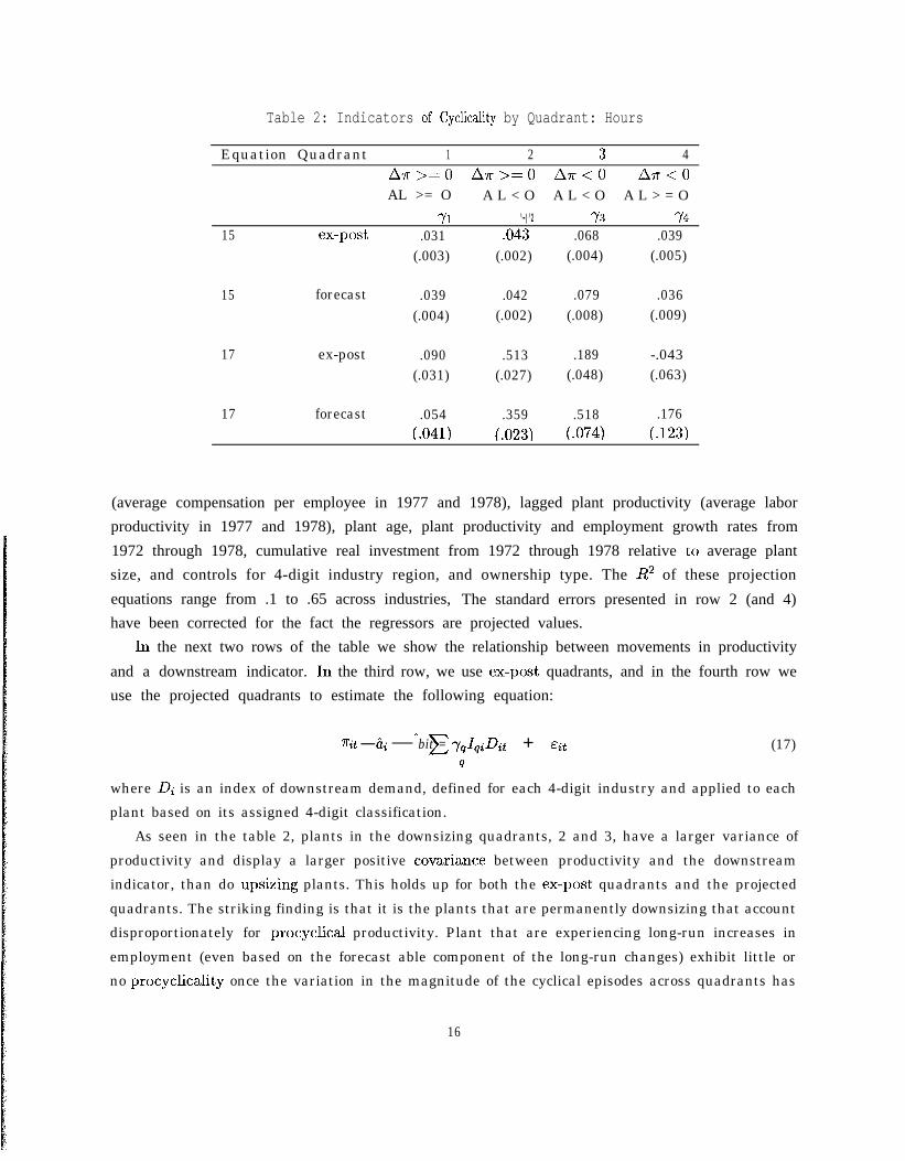
Table 2: Indicators of Cyclicality by Quadrant: Hours

Equation Quadrant 1 2 3 4Ax>=O Am>=O An<O An<OAL >= O A L < O A L < O A L > = O

w ‘-)’2 -n 7415 ex-post .031 ,043 .068 .039

(.003) (.002) (.004) (.005)

15 forecast .039 .042 .079 .036(.004) (.002) (.008) (.009)

17 ex-post .090 .513 .189 -.043(.031) (.027) (.048) (.063)

17 forecast .054 .359 .518 .176(.041) (.023) (.074) (.123)

(average compensation per employee in 1977 and 1978), lagged plant productivity (average labor

productivity in 1977 and 1978), plant age, plant productivity and employment growth rates from

1972 through 1978, cumulative real investment from 1972 through 1978 relative to average plant

size, and controls for 4-digit industry region, and ownership type. The 112 of these projection

equations range from .1 to .65 across industries, The standard errors presented in row 2 (and 4)

have been corrected for the fact the regressors are projected values.

In the next two rows of the table we show the relationship between movements in productivity

and a downstream indicator. 111 the third row, we use ex-post quadrants, and in the fourth row we

use the projected quadrants to estimate the following equation:

“ ~~qL+D,, + E,,nit — ai — bit = (17)9

where lli is an index of downstream demand, defined for each 4-digit industry and applied to each

plant based on its assigned 4-digit classification.

As seen in the table 2, plants in the downsizing quadrants, 2 and 3, have a larger variance of

productivity and display a larger positive covariance between productivity and the downstream

indicator, than do upsizing plants. This holds up for both the ex-post quadrants and the projected

quadrants. The striking finding is that it is the plants that are permanently downsizing that account

disproportionately for procyclical productivity. Plant that are experiencing long-run increases in

employment (even based on the forecast able component of the long-run changes) exhibit little or

no procyclicality once the variation in the magnitude of the cyclical episodes across quadrants has

16

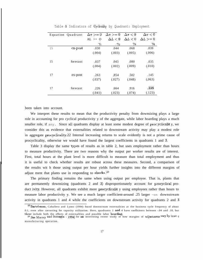
Table 3: Indicators of Cyclicality by Quadrant: Employment

Equation Quadrant An>=O Ax>=O Ar<O Ar<OAL >= O AL<O AL<O AL>=O

71 7’2 -)2 7415 ex-post .030 .044 .068 .039

(.004) (.003) (.005) (.006)

15 forecast .037 .043 .080 .035(.004) (.002) (.009) (.010)

17 ex-post .263 ,854 .502 .145(.037) (.027) (.048) (,063)

17 forecast .226 .664 .916 .338(.041) (.023) (.074) (.123)

been taken into account.

We interpret these results to mean that the productivity penalty from downsizing plays a large

role in accounting for pro cyclical productivity y of the aggregate, while labor hoarding plays a much

smaller role, if any. Since all quadrants display at least some modest degree of proc yclicalit y, we

consider this as evidence that externalities related to downstream activity may play a modest role

in aggregate procyclicality. 22 Internal increasing returns to scale evidently is not a prime cause of

procyclicality, otherwise we would have found the largest coefficients in quadrants 1 and 3.

Table 3 display the same types of results as in table 2, but uses employment rather than hours

to measure productivity. There are two reasons why the output per worker results are of interest.

First, total hours at the plant level is more difficult to measure than total employment and thus

it is useful to check whether results are robust across these measures. Second, a comparison of

the results wit h those using output per hour yields further insights into the different margins of

adjust ment that plants use in responding to shocks .23

The primary finding remains the same when using output per employee. That is, plants that

are permanently downsizing (quadrants 2 and 3) disproportionately account for procyclical pro-

duct ivity. However, all quadrants exhibit more procyclicalit y using employees rather than hours to

measure labor productivity y. We see a much larger coefficient-around .25 larger —on downstream

activity in quadrants 1 and 4 while the coefficients on downstream activity for quadrants 2 and 3

22 Bartelsman, Caballero and Lyons (1994) found downstream externalities at the business cycle frequency of about0.1, even after correcting for capacity utilization. Here, quadrants 1 and 4 have coefficients between -.04 and .18, butthese include both the effects of externalities and possible labor hoadng.

23 see Mattey and stron~in ( Igg4) for an interesting recent study of how margins of adjustnlent varY bY tYPe ‘f

manufacturing operation.

17

are about .3 higher than in the output per hour table. This result reflects the Well-kIlOW1l finding

that hours per worker fall in recessions.

The fact that the difference between the cyclicality of output per worker and olltput per hour

are about the same for all quadrants suggests that it is not labor hoarding which motivates plants

to adjust hours per worker downwards in recessions. For if this were the case, then following the

arguments discussed above, it should be in quadrants 1 and 4 that this effect should be especially

important. Inst cad, this result indicates that all quadrants exhibit similar proc yclicalit y in hours

per worker. Apparently, adjusting to an adverse cyclical shock in part by reducing hours per worker

is common across plants with quite different long-run prospects.24

6 c o n c l u s i o n s

ln t his paper, we exploit the cross sectional variation in long-run structural changes across plants to

distinguish between different hypotheses for explaining the observed procyclicality of labor produc-

tivity. Using a large balanced panel of all continuously operating plants in the U.S. manufacturing

sector during the 1970s and 1980s, we find that it is plants that are permanently downsizing that

disproportionately account for procyclical productivity. Plants that are upsizing in the long run

exhibit little or no procyclical productivity. These results favor an adjustment cost model which

involves a productivity penalty for downsizing ZM the largest source of pro cyclical labor productiv-

ity y, although a modest role may be played by external economies. Internal increasing returns and

labor hoarding appear to play little role, if any, in the Procyclicality of productivity.

There are a number of directions that these striking findings could be explored further in future

research. First, the role of capital adjustments in the dynamics of employment and labor produc-

tivity is an area of obvious interest. In addition, incorporating capital into the theoretical and

empirical analysis would permit replication of our results for measures of total factor productivity.

Second, our empirical approach has been descriptive and non-parametric rather than structural.

In principle, it would be interesting to estimate a structural model that fully nests the competing

hypotheses and that would allow a clean, precise decomposition of the factors accounting for pro-

cyclical productivity. However, we are a long way from being able to undertake this formidable task

in this environment that stresses the interaction of plant-level heterogeneity y, long-run structural

changes and cyclical variation.

24As suggested by the analysis of Bils (1987), Caballero and Engel (1993), and Caballero, Engel and Halti-wanger (1994), the costs of varying hours per worker and varying the number of workers is influenced by a number offactors. Consistent with the findings reported here, Caballero, Engel and Haltiwanger (1994) find that plants adjustto shocks first by changing hours per worker and only change the number of employees once the deviation betweenact ual and desired employment becomes sufficiently kwge.

18

R e f e r e n c e s

Abraham, Katherine and John Haltiwanger, “Real Wages and the Business Cycle,” Journal

of Economic Literature, 1995, 33.

Aizcorbe, Ana M., “Procyclical Labour Productivity, Increasing Returns to Labour, and Labour

Hoarding in Car Assembly Plant Employment ,“ Economic Journal, .July 1992, 102 (413),

860-73.

Baily, Martin N., Charles Hulten, and David Campbell, “The Distribution of Productivity

in Manufacturing Plants, “ in ‘~ Brookings Papers: Macroeconomics” Washington, D .C. 1992.

—? Eric J. Bartelsman, and John Haltiwanger, “Downsizing and Productivity Growth:

Myth or Reality,” in David G. Mayes, ed., Sources oj Productivity Growth in the 1980s,

Cambridge: Cambridge University Press, 1995.

Bartelsman, Eric J. and Phoebus J. Dhrymes, “Productivity Dynamics: US. Manufacturing

Plants 1972- 1986,” FEDS 94-1, Federal Reserve Board .January 1994.

and Wayne Gray, “The NBER Manufacturing Productivity Database,” July 1995. mimeo.

_ , Ricardo J. Caballero, and Richard K. Lyons, “Customer and Supplier Driven Exter-

nalize s,” American Economic Review, September 1994, 34 (844), 1075-84.

Bean, Charles R., “Endogenous Growth and the Procyclical Behavior of Productivity,” European

Economic Review, May 1990, 34 (2-3), 355-63.

Bentolila, Samuel and Giuseppe Bertola, “Firing Costs and Labor Demand: How Bad is

Eln-osclerosis’!,’) Review of Economic Studies, 1992, 57, 381-402.

Bernanke, Ben and Martin Parkinson, “Procyclical Labor Productivity and Competing The-

ories of the Business Cycle: Some Evidence from Int erwar U.S. Manufacturing Industries,”

Journal of Political Economy, .June 1991, 99 (3), 439-59.

Bils, Mark, “The Cyclical Behavior of Marginal Cost and Price,” American Economic Review,

December 1987, 77 (5), 838-55.

Brechling, Prank, Investment and Employment Decisions, Manchester: Manchester University

Press, 1975.

Burnside, Craig, Martin Eichenbaum, and Sergio Rebelo, “Labor Hoarding and the Busi-

ness Cycle,” Journal of Political Economy, April 1993, 101, 245-73.

—9— , and _ 1 “Capital Utilization and Returns to Scale,” February 1995. mimeo.

19

Caballero, Ricardo and Eduardo Engel, “Macroeconomic Adjustment Hazards and Aggregate

Dynamics,” Quarterly Journal of Economics, May 1993, 108 (2), 313-58.

Caballero, Ricardo J., Eduardo M.R.A. Engel, and John Haltiwanger, “Aggregate Em-

ployment Dynamics: Bllilding from Macroeconomic Evidence,” working paper 5042, NBER

February 1994.

Davis, Steve and John Haltiwanger, “Gross .Job Creation and Destruction: Macroeconomic

Evidence and Macroeconomic Implications,” in “NBER Macroeconomics Annual, V“ 1990,

pp. 123-68.

Fair, Ray C., The Short-run Demand for Workers and Hours, Amsterdam: North-Holland, 1969.

Fay, J. and James Medoff, “Labor and Output Over the Business Cycle,” American Economic

Review, 1985, 75, 638–55.

Gordon, Robert J., “Are Procyclical Productivity Fluctuations a Figment of Measurement Er-

ror,>’ 1990. Northwestern University.

Griliches, Zvi and Regev, Haim, “Productivity and Firm Turnover in Israeli Industry: 1979-

1988,” working paper 4059, National Bureau of Economic Research April 1992.

Hall, Robert E., “The Relation between Price and Marginal Cost in U.S. Industry,” Journal of

Political Economy, October 1988, 96, 921-47.

—1 “Econometric Research on Shifts of production Functions at Medium and High Frequencies,”

August 1990. presented at Barcelona World Congress of the Econometric Society.

Hamermesh, Daniel and Gerald Pfann, “Adjustment Costs in Factor Demand,” October 1994.

mimeo.

Kuh, Edwin, “The Brookings Quarterly Econometric Model of the United States,” in .James

Duesenberry, Gary Fromm, Lawrence Klein, and Edwin Kuh, eds., income Distribution and

Employment Ouer the Business Cycle, Chicago: Rand McNally, 1965.

Mattey, Joe P. and Steve Strongin l “Factor Utilization and Margins for Adjusting Output:

Evidence from Manufacturing Plants,” November 1994. mimeo.

Oi, Walter Y., “Labor as a Quasi-Fixed Factor,” Journal of Political Economy, December 1962,

70, 538-55.

Saint-Paul, Gillesl “Productivity Growth and the Structure of the Business Cycle,” European

Economic Review, May 1993, 37 (4), 861-83.

20

Sargent, Thomas, “Estimation of D ynamic Labor Demand Schedules Under Rational Expecta-

tions, )’ Journal of Political Economy, 1978, 86, 1009-1044.

Shea, John, “DO Supply Curves Slope Up?,” Quarterly Journal of Economics, 1993, 108 (l), 1-32.

Solow, Robert M., “Some Evidence on the Short-Run Productivity Puzzle,” in .J. Baghwati and

Eckaus R. S., eds., Development and Planning, London: Allen and Unwin, 1973, pp. 317-25.

21

7 A p p e n d i x A – D e t a i l s o f T h e o r e t i c a l R e s u l t s

7.1 Labor Hoarding

The key result for this section is that mat is increasing in g: and g$. This result can be derived

by rearranging equations (7) and (8) which yields Wt = (~13[&+l Ait+l (F2it+l ) + (1 – di)wt+l]).

In order to satisfy this relationship and equation(7) for period t+ 1, an increase in expected future

~it+ 1 Ait+l must be met by an increase in m~t.

This resldt implies that, other things equal, establishments with more favorable future demand

and technology conditions are more likely to hoard labor in response to a current adverse demand

shock. (hlsider two plants with identical hitiid and cllrrent conditions but one with higher ex-

pected growth in demand and technological progress. By identical initial conditions, we mean

they both have the same prior period employment and maintenance capital. By the same current

~O1lditiOIIS we mean that hot h face the same adverse current demand shock. Thus, by (7), both

plants will employ the same amount of labor directly in production. However, the plant with more

favorable future conditions will have higher m~t.

7.2 Adjustment Costs

The central result of this section is that an establishment will reduce employment by a greater

amolmt in response to an adverse current demand shock (represented by a lower Pit) the lower is

the expected future growth of demand and technology (represented by a lower ~~t+l and Ait+l ).

This result is derived most easily in the extreme. Consider two plants that face identical initial and

mlrrent conditions with both making layoffs this period due to a low current realization of demand.

However, suppose one has sufficiently positive anticipated growth in demand that it will be hiring

next period with certainty, but the other has sufficiently negative anticipated growth in demand

that it will be laying off workers with certainty next period. Inspection of (12) across these two

extremes immediately yields that the plant that k contracting in the future will make more layoffs

in the mmrent period. The same basic logic applies in the less extreme case.

22

. ,.

Chart 1: LRD Sample vs. All Manufacturing

- 4000All Mfg. -,.... . . %. m

. ..- . . .,.. . . . . 3-.. . ,... . . . ‘ . . . ..-,. q. . . --- ----.,. . 0,.,‘. ,.‘. ., 3600 j‘. ,,.‘... I

oc

-------- Employment7

1600 1 I , I , I , I I , I , I , I ,I 3200

73 75 77 79 81 83 85 87

1250 r 1 1600

I LRD Sample~ 1150U1 -% . . . . . .q ● ~rn -.

●.-. . . . . .#--- ..,.,....- . . .

I l l

!’;[ *-:~:J .~-----------------------,------- j“nnt

1200

. ..-/ -I

, .“” 03

- - - - - - - - Fmnlnvment . . ,. . . . . . . . .--—I UJ. . . . . . . ..- -.

750 1 I , I , I r I , I , 1 , I , I I

73 75 77 79 81 83 85 87

10.0[

1~-’,.. ,,..

5.0 . . . , . . . . . . . .. . . ,.’ . . .. . . . . . . . . --- ,,. . . . ..-” . . . .. . . . . .--”,.,’ ,.,. . . . . . . ...-. . . ,, . -----,, ..-. ..”... . ,, -- . . . . . .-.. . ..- . . ,,,..,, . . . . ‘..%... ,.,. . . . . . . ..-

0.0‘.. . . . .‘.. ,.=’‘.. .. — A l l Mfg

-------- LRD

-5.0 I I I I I I I I I

73 75 77 79 81 83 85 87

10.00

5.00

0.00

-5.0072

Chart 2: Productivity Decomposition: within plant and mix effectsFull LRD Sample

. ..,,,.,,.,

. . .

— Z$., ,A~,, productivity (within plants)--------- Zn_l’lA$t, employment share--- XAnlA$,, cross term

I I I I I I I I 1

74 76 78 80 82 84 86 88year

I I

.—“.‘.‘.,

‘.‘.,.,

,.,.,

,.,. . .

‘.‘.‘.:

ba)

u)co

mco

z

a l1=

-..:‘. m::‘.‘.

‘..‘..

n . .‘.:‘.‘,‘. Ww,,

,,.,,

,’,’

,“,’

=

u ,,”

I I I,. I

1

Ww

bb r’,.

>

. . .. . .

. .. . . . .. .. . . .. . . .. .

.,””. . ....

,,,;

=—u