LABOR RATIONING: A REVEALED PREFERENCE APPROACHFROM HIRING SHOCKS

EMILY BREZA?, SUPREET KAUR‡, AND YOGITA SHAMDASANI†

Abstract. Assessing unemployment levels is empirically challenging. Economistscurrently rely on survey self-reports, whose reliability is unknown and which make itdifficult to disentangle those who have exited the labor force and the self-employedfrom rationed workers. In this paper, we develop an approach to obtain the firstrevealed preference estimates of labor rationing. We generate large transitory hiringshocks in Indian local labor markets — hiring up to 35% of the male labor force formonth-long work in external factories. We examine the impact of these transitoryshocks on the local labor market to diagnose the extent of rationing. We find evidencefor severe labor rationing during lean seasons, which account for 6 months of the year.Specifically, “removing” a large portion of workers leads to (i) no change in the localwage, and (ii) no change in local aggregate employment levels (excluding our exter-nal jobs); this is due to one-for-one positive employment spillovers on the remainingworkers who benefit from decreased competition for job slots. We further decomposerationing into involuntary unemployment and disguised unemployment (self-employedworkers who would prefer wage labor). In contrast, we detect limited evidence forlabor rationing during peak employment seasons: in these months, transitory exter-nal hiring shocks increase local wages and reduce local aggregate employment. Inaddition, we show that traditional government surveys substantively underestimateunemployment in this setting. This approach can be extended to obtain revealedpreference bounds on involuntary unemployment in diverse settings.

Date: This Version: August 12, 2019.We thank Abhijit Banerjee, Pat Kline and many seminar participants for helpful comments andconversations. We thank Arnesh Chowdhury, Piyush Tank, Silvia Wang, Mohar Dey, AnshumanBhargava, Vibhuti Bhatt, Asis Thakur, and Anustubh Agnihotri for excellent research assistance.?Department of Economics, Harvard University; NBER; JPAL.‡Department of Economics, University of California Berkeley; NBER; JPAL.†Department of Economics, University of Pittsburgh.

LABOR RATIONING 1

1. Introduction

[D]istinguishing elements of voluntariness from elements of involuntari-

ness in the unemployment problem is a hopeless endeavour. (Fellner,

1976)

Early work in development economics took seriously the notion that a large fraction

of the rural workforce is unemployed. Research in the 1950s and 1960s — based

on survey data — posited that rural labor markets appear to not clear, resulting in

excess labor supply (e.g., Lewis, 1954; Eckaus, 1955; Leibenstein, 1957). This notion

has potential relevance today. For example, agricultural workers in India report having

agricultural employment on only 44% of days during the year (National Sample Survey

(NSS), 2009). However, the official rural unemployment rate from the same survey was

only 1.6%.

Such survey statistics are difficult to interpret. Is the non-employment voluntary or

involuntary? Are workers who report self-employment in household enterprises fully

employed, or is this “disguised unemployment” — a form of under-employment and

a response to being rationed out of the labor market? Identifying the true levels of

involuntary un- and under-employment is crucial for understanding the functioning of

rural labor markets.

The challenge of measuring unemployment pertains to rich and poor countries alike.

To date, economists have measured unemployment using survey self-reports, whose re-

liability is uncertain (Taylor, 2008; Card et al., 2012). For example, survey respondents

asked for retrospective labor market information are likely to over-estimate employment

and under-estimate unemployment spells (Bowers and Horvath, 1984; Mathiowetz and

Ouncan, 1988). Moreover, underemployment complicates any labor market analysis

(Ham, 1982). In addition, people may not be qualified.

LABOR RATIONING 2

In this paper, we overcome these challenges by developing a revealed preference

approach to test for and quantify labor rationing. We define a worker to be rationed out

of the labor market if he satisfies two conditions: a) he would prefer wage employment

(at the existing market wage for that job) over what he is currently doing (i.e. the

worker is not on his labor supply curve), and b) the worker is employable at that wage

(i.e. from the employer’s perspective, his marginal product is above the current market

wage for the job).

The setting for our test is rural labor markets in Odisha, India, which mirror the

seasonality found in most low-income, rural settings. Specifically, we exploit an oppor-

tunity to recruit workers for 2-4 week-long employment in external factories. We use

this to generate transitory aggregate hiring shocks in (random) villages — absorbing

up to 35% of the labor force of casual male workers. To test for rationing, we examine

how this external hiring shock affects wages and employment in the local village labor

market. We conduct this test across different months of the year, which correspond to

different levels of labor market demand and employment.

If the amount of labor rationing is weakly greater than the size of the external hiring

shock, then we predict the hiring shock will have the following effects among workers

who remain in the village (i.e. were not removed due to the hiring shock): L1) no effect

on local wages; L2) positive employment spillovers — higher individual employment

(due to reduced competition for job slots); and L3) no effect on aggregate employment

levels. In contrast, if the hiring shock is larger than the amount of rationing (e.g. if

there is no labor rationing), then such a hiring shock should produce: P1) an increase

in local wages; and P2) a decrease in aggregate employment among workers who re-

main in the village. Note that this constitutes a revealed preference test for rationing.

Specifically, if predictions L1-L3 hold, workers reveal that they prefer jobs at the mar-

ket wage over their previous activity (e.g. unemployment or self-employment), and

LABOR RATIONING 3

employers reveal that the worker is qualified to be hired for that job at the market

wage.

A benefit of this approach is that it uncovers labor market functioning without

direct intervention on the participants of interest. While we exogenously generate hir-

ing shocks, the outcomes of interest are driven completely by the local response of

existing employers and workers who never interface with the external factories. We

simply “remove” some workers, and examine what the labor market does in response.

In addition, examining who benefits from employment spillovers can be used to de-

compose rationing into two components: involuntary unemployment and disguised

unemployment. Finally, we compare our revealed preference estimates with a series of

traditional self-reported survey-based measures of unemployment.

We conduct the experiment using a matched-pair, stratified research design in 64

labor markets (i.e. villages) across varying times of the year. We invite workers to sign

up for employment at the external factories, which reflect desirable manufacturing jobs

with higher wages — leading to signups by a large proportion of the labor force.1 We

then randomly choose from among sign-ups to pick which workers are “removed”. On

average, we hire 24% of the labor force of male workers in treatment villages. We use

employment rates in the non-treated villages as our proxy for underlying labor market

slack; using this measure, we classify hiring rounds as falling under peak or lean periods

of the year.

Our results highlight two stark facts about the functioning of rural labor markets

in our setting. First, they provide strong support for high levels of rationing during

lean seasons (which account for about 6 months of the year). Second, they highlight1Note that since our tests are based solely on how local wages and employment respond to our shocks,offering a wage higher than the prevailing wage for our external jobs is not a problem for our test.Rather, it provides benefits by enabling us to draw workers from across the skill distribution in thevillage.

LABOR RATIONING 4

the importance of seasonality: during peak times, the labor market response to shocks

corresponds to what one would expect under market clearing conditions.

Specifically, consistent with Prediction L1, we find no evidence that wages in the

village change in response to an external hiring shock in lean months. However, in

peak months, the hiring shock raises local wages by 0.0545 log points (p-value 0.0179),

on average (Prediction P1). These results hold across samples of workers, both those

who signed up for the jobs and the full village (including those who did not sign up for

the external jobs) — indicating a rise in equilibrium wages.2

We next analyze the spillover impacts of the hiring shock on the individuals remain-

ing in the village. Specifically, we consider the workers who signed up for but were not

randomly given employment at the external factories — i.e. the “spillover sample”.3

In the lean months, we find substantial spillover impacts — the likelihood of wage

employment increases by 0.0552 percentage points (p-value 0.004) on a base rate of

wage employment of 0.145 (Prediction L2). This is consistent with our prediction that

workers who were previously rationed fill in job slots when their peers are “removed”

from the labor market. In contrast, we cannot reject that there are no employment

spillovers onto the remaining workers in the peak season.

Finally, to test Prediction L3, we measure impacts on aggregate employment levels

(excluding our external worksite jobs). For this, we sum employment across all workers

in the labor market — those who signed up for our jobs and those who did not.

Consistent with Prediction L3, there is no change in local aggregate employment in

the lean season. This follows from the previous two predictions. Because wages do

not change in the lean season, labor demand by employers remains the same; rationed

workers fill in these job slots, leading to the same level of aggregate employment in the2In addition, we document that there are no significant differences in worker characteristics amongthose who receive jobs in treatment vs. control villages. This provides further evidence against aninterpretation of these results that is driven by compositional changes in who is getting employed.3Given that this group is directly comparable to the workers who were removed from the village, wewould expect to find the largest spillovers onto them.

LABOR RATIONING 5

village. In other words, creating external jobs for up to 35% of workers generates no

crowd-out in the private labor market in the lean season.

In contrast, consistent with Prediction P2, the hiring shocks lead to a decrease in

aggregate employment in the peak season. Workers in villages that experienced hiring

shocks experience a 0.040 percentage points (p-value 0.002) decline in employment on

a base rate of wage employment of 0.198. In the peak season, every job that we create

in our external factories crowds out 0.149 days (p-value 0.0659) of local labor market

employment.

We further decompose rationing into involuntary unemployment and disguised unem-

ployment (self-employed workers who would prefer wage labor). A large body of work

in development has highlighted that rationed individuals may turn to less-productive

self-employment as a way to generate income — creating “disguised unemployment”

or “underemployment” (e.g., Singh et al., 1986; Benjamin, 1992). In accordance with

this, in response to hiring shocks in lean months, workers switch from self-employment

to wage employment when jobs become easier to find. Self employment declines by a

large margin: 0.0390 percentage points on a base of 0.13 (p-value 0.031). This accounts

for an estimated 71% of the employment spillovers.

Finally, we estimate the impacts of the hiring shock on self-reported involuntary

unemployment. For this, we examine two measures of involuntary unemployment.

First, we measure effects on the traditional measure used in government surveys across

a range of settings (e.g. India and the US).4 This traditional approach only codes

workers as involuntarily unemployed if they report no other work activity. Under this

measure, we fail to find significant changes on lean season involuntary unemployment as

a result of the hiring shocks. Given the importance of disguised unemployment in our4Our elicitation follows the same procedure as the Indian National Sample Survey. The US LaborBureau also follows the approach where if a worker reports self-employment, they cannot be classifiedas involuntarily unemployed.

LABOR RATIONING 6

setting, this is not surprising — many workers who appear gainfully employed in self-

employment are actually involuntarily rationed out of the wage labor market. Second,

we propose an alternate measure that allows workers to state whether they would

have preferred wage employment rather than their activity on a given day. Using this

measure, involuntary unemployment falls by 0.553 percentage points (p-value 0.045).

This corresponds closely to our estimated spillover effects, indicating that this survey

measure approximates the magnitude of the revealed preference response.

Our design enables us to rule out a series of potential concerns that may confound

the interpretation of the above results. First, if labor supply is perfectly elastic, this

could generate predictions L1-L3 even in the absence of rationing. We exploit data from

Breza et al. (2019), in which workers are offered jobs by existing agricultural employers

at random wage levels. There is substantive labor supply below the prevailing wage,

ruling out perfectly elastic supply. In addition, in the experiment in this paper, our

wage and employment spillover results from the lean months would require a labor

supply elasticity of 5.6 - 27.4 to rationalize our findings.5 This is implausibly high,

and is substantively higher than the estimated labor supply elasticity in Breza et al.

(2019).

Second, we test whether the lack of an effect on aggregate employment and the shifts

out of self-employment might in part be driven by workers postponing self-employment

activities. We return to the respondents two weeks after the end of the labor supply

shock and find no lasting impact on employment levels in the lean season. Moreover,

self employment activities, if anything, remain depressed even after the end of the

supply shock.

Third, one might wonder if the lack of a response in the wage might be due to changes

in the composition of available workers due to the labor supply shock. However, even

if the average worker quality does change, our estimates still provide a lower bound5For this, we take the right hand side of the 95% confidence interval of the wage point estimate andthe 95% confidence interval of the employment spillover results in the lean season.

LABOR RATIONING 7

estimate of the level of rationing. Importantly, by revealed preference, any worker that

receives positive spillovers from the labor supply shock must be sufficiently productive

to be employed at the market wage rate. Given that in the lean season, the hiring

shock does not affect wages, quality concerns do not change our conclusions about the

extent of labor rationing. Importantly, our design does not require us to take a stance

on the labor allocation mechanism in the presence of rationing.

A few additional caveats are in order when interpreting our findings. Clearly, the

magnitudes of our estimates are only relevant to our specific context of rural Odisha.

However, we do believe that the methodology and problem of measuring involuntary

un- and under-employment has much broader relevance, spanning both rich and poor

countries. In our particular context, two different labor market paradigms are relevant,

depending on predictable fluctuations in employment levels. Similar dynamics are likely

to prevail in many rural, developing country settings. We also note that our design

neither explains nor requires an explanation for the microfoundation for rationing (see

Breza et al., 2019).

Our paper speaks directly to several different literatures. First, we add to a long

line of research analyzing rural labor markets in developing countries. As we mention

above, early work posits severe distortions in the labor market, including surplus la-

bor, rationing, and separation failures (Lewis, 1954; Eckaus, 1955; Leibenstein, 1957).

However, a subsequent wave of research documents wage adjustment to shocks, which

many point to as evidence inconsistent with severe distortions (Rosenzweig, 1988; Jay-

achandran, 2006; Imbert and Papp, 2015; Breza and Kinnan, 2018). These conflicting

findings and viewpoints have made it difficult to characterize the functioning of rural

labor markets. We provide the first experimentally-identified evidence of the magni-

tude of labor rationing in a rural developing country setting. In addition, we reconcile

the two strands of this literature by showing that the labor market effects of shocks

LABOR RATIONING 8

depend heavily on seasonality: wage and employment adjustment happens quickly in

peak seasons.

Second, this paper also relates to recent work on general equilibrium impacts of

shocks relevant to labor markets (Donaldson and Keniston, 2016; Muralidharan et al.,

2017; Akram et al., 2017). These papers typically find evidence of wage responses. Our

results are consistent with these types of effects, but we also show that crucially, the

extent to which wages might respond will depend on whether the shock is limited to lean

employment periods or also overlaps with peak times of the year. Our methodology is

closely related to Crepon et al. (2013), who vary the intensity of job placement services

(a supply shock) across French labor markets to test for displacement effects. They find

evidence that direct gains from the treatment come at the expense of other non-treated

workers in their same labor market. They also find evidence that underlying market

conditions are key mediators of displacement effects. Because our hiring shocks are

so large, we are able to take this methodology one step further and test for aggregate

impacts on the whole labor market, and in our context, measure the extent of rationing.

Finally, as discussed above, our paper relates to the labor economics literature on

measuring unemployment. Perhaps unsurprisingly, we show that the standard survey

methodology for eliciting involuntary unemployment does not match our revealed pref-

erence estimates. We propose a new way to elicit involuntary unemployment in surveys

and empirically validate it in our context. We believe that this could be especially use-

ful in settings with high potential for disguised unemployment or underemployment

(e.g., high rates of small-scale self-employment).

The remainder of the paper is organized as follows. Section 2 describes the context

and setting. Section 3 outlines our empirical predictions, alternately, under market

clearing and under labor rationing. Section 4 details the experimental design and its

implementation. Section 5 describes the data. We present the experimental results

LABOR RATIONING 9

in Section 6. Section 7 discusses potential threats to validity. Section 8 provides a

discussion.

2. Context

The experiment takes place in villages across five districts in rural Odisha, India.

Markets for casual daily labor are extremely active in this setting.6 Daily-wage workers

engage primarily in rainfed agriculture for approximately six months of the year. In

the remaining lean months, they typically seek short-term contract employment in

non-agriculture, such as manufacturing and construction.

The village constitutes a prominent boundary for the casual labor market — daily-

wage workers typically find work in both agriculture and non-agriculture within or

close to their own village. For example, among workers in our study sample, 70%

and 46% of reported worker-days in agriculture and non-agriculture respectively are

for work within the village. For work outside the village, the median distance from

own village is 3 kilometers for agricultural employment, and 4 kilometers for non-

agricultural employment. Further, hiring is largely employer-directed — employers

approach workers for 88% of reported worker-days, while workers approach employers

for only 5% of reported worker-days.

Figure 1 illustrates the average daily employment rate for casual work in our study

villages. Employment rates are generally low; the mean daily employment rate, re-

stricting to hired wage employment only, is 17%. Further, employment rates are

highly variable. The mean daily employment rate falls to 13% in the lean months,

which spans approximately half the year, and rises to 21% in the peak months. The

villages in our study thus match a general feature of village economies: large periods

of low employment.6Markets for casual daily labor are ubiquitous across poor countries. They constitute an employmentchannel for hundreds of millions of workers in India alone, and account for 98% of the country’s hiredagricultural labor (National Sample Survey, 2010). Casual labor markets are characterized by a highdegree of decentralization and informality (e.g. Rosenzweig, 1988).

LABOR RATIONING 10

3. Hypotheses

3.1. Definition of Labor Rationing. Suppose the prevailing wage for one day of

work in the casual daily market is w. We define a worker as rationed on a given day

when the following two conditions hold: (i) The worker wants to supply labor at wage

w, but is unable to find employment; (ii) The worker is qualified for jobs occupied by

other villagers.

The first condition essentially states that the worker is not on her labor supply curve.

The second condition states that a worker who wants a job but is unqualified for it (in

the sense that an employer would never find it profitable to hire her at wage w) is not

considered rationed. Note that we take no stance on neither the micro-foundation nor

the mechanism for rationing. Our goal is to quantify rationing, and decompose it into

involuntary unemployment and disguised unemployment.

3.2. Predicted Impacts of a Negative Labor Supply Shock. Our field exper-

iment is designed to exogenously shock village labor supply. This is achieved using

an experimental hiring shock, where a subset of workers in the local labor market are

hired in external jobs generated outside the village. By removing workers from the

village, the shock leads to a reduction in the residual labor supply remaining in the

village, while local labor demand remains unchanged. We then examine what happens

in the local labor market after the negative supply shock.

In laying out our predictions, we employ the simplest framework to interpret our

results: a stylized demand and supply framework. Panel A of Figure 2 shows the

effects of a negative labor supply shock under market clearing. Let E denote the level

of employment (in terms of worker-days) in the village and w denote the village wage in

the absence of our intervention. A negative supply shock (a shift from S to S ′) should

lead to: P1) an increase in local wages from w to w′; and P2) a decrease in aggregate

LABOR RATIONING 11

employment among workers who remain in the village (i.e. those who are not hired by

us to work in factories), so that total employment after the shock E ′ < E.

Panel B of Figure 2 shows the effects of a negative labor supply shock under a wage

floor. As before, E denotes the level of employment in the village and w denote the

village wage in the absence of our intervention. Rationing exists in this labor market,

with supply ES exceeding demand ED at wage w. If the amount of labor rationing is

weakly greater than the size of the supply shock, then we predict that a negative supply

shock (a shift from S to S ′) should lead to: L1) no effect on local wages; L2) positive

employment spillovers among workers who remain in the village — higher individual

employment (due to reduced competition for job slots); and L3) no effect on aggregate

employment levels. If predictions L1-L3 hold, workers reveal that they prefer jobs at

w over their previous activity (e.g. unemployment or self-employment), and employers

reveal that workers are qualified to be hired for the jobs at w — this thus constitutes

a revealed preference test for rationing.

Note that predictions L2 and L3 above are inherently related. The amount of ra-

tioning equals ES − ED, in terms of worker-days. With the supply shock, a set of

workers in the village achieves full employment in the factories. This generates em-

ployment spillovers on the remaining workers (i.e. those who are not hired by us to

work in factories), because a larger fraction of them can fill the available job slots (in

terms of worker-days) in the local village labor market (Prediction L2). However, as

long as the amount of labor rationing is weakly greater than the size of the negative

supply shock, then total employment (i.e. total worker days hired by employers) in the

local village labor market will not change (Prediction L3).

To illustrate these predictions, consider the following thought exercise. Suppose 10

workers want to work in the village for wage w, but only 5 job slots are available at

this wage. As a result, 5 workers are employed at wage w, while the other 5 workers

are rationed (50% employment). Now, suppose we remove 4 workers from the village

LABOR RATIONING 12

labor market. This frees up job slots, and a larger portion of the remaining workers

can work in the village labor market at wage w. Specifically, there are 6 workers left

who want work and 5 available slots (83% employment). In contrast, if the 5 workers

who are unemployed did not want work, they would not accept employment at wage

w; this provides a test of condition (i) above. In addition, the fact that workers who

remain in the village are hired at wage w indicates that employers perceive them as

qualified for work at w; this gives a test for condition (ii) above.

Our predictions above do not require us to take a stance on how the composition of

workers — in terms of ability — changes as a result of the supply shock. There may

be a distribution of ability levels among rationed workers. However, for us to observe

employment spillovers (Prediction L2), it must be the case that the rationed workers

are qualified for work at wage w.

3.3. Decomposing Rationing. If there is labor rationing — supply exceeds demand

at wage w — then not all workers who would like to work at wage w will find work.

Individuals who are rationed may appear as unemployed or may turn to less-productive

self-employment as a way to generate income — creating disguised unemployment or

“forced entrepreneurs” (Singh et al., 1986). For these “forced entrepreneurs”, self-

employment earnings are below w, but above their reservation wage.

We test the extent to which the supply shock induces a subset of self-employed indi-

viduals to prefer wage employment at w, thus identifying themselves through revealed

preference as “forced entrepreneurs”. We predict that under rationing, a negative sup-

ply shock will lead to a reduction in worker-days in self-employment for workers who

remain in the labor force (i.e. those who are not hired by us to work in external jobs).

4. Experiment: Design and Implementation

4.1. Experimental Labor Supply Shocks. We engineer transitory aggregate supply

shocks in our study villages. In doing so, we exploit an opportunity to recruit casual

LABOR RATIONING 13

male workers for full-time employment in low-skill manufacturing jobs for a one-month

period. The work takes place in external factories that are within daily commuting

distance from the villages.7 These month-long contract jobs are attractive to workers

— the daily wage paid is weakly higher than the prevailing market wage for casual

labor, and there are positive compensating differentials as the work takes place indoors

and is not very physically demanding.

Several days prior to the first day of work, jobs at the external factories are advertised

in villages through the distribution of flyers, village meetings, and door-to-door visits.

During this time, male workers interested in the job are encouraged to sign up. Hired

workers are then drawn randomly from this subset of the village labor force that signs

up for the job.

We randomize recruitment at the village (i.e. labor market) level, so that in treat-

ment villages we hire up to 60% of the male workers who sign up, and in control

villages we hire 1-5 male workers who sign up. We thus generate a large hiring shock

in treatment villages, and a negligible hiring shock in control villages. By varying the

intensity with which we recruit workers across villages, we generate exogenous varia-

tion in village-level residual labor supply. We use a matched-pair, stratified research

design, so as to achieve balance by local region and time.

To test our predictions, we examine the impact of this external labor supply shock

on wages and employment in the local village labor market. We conduct this test

in different months of the year, which correspond to different levels of labor market

demand and employment. We use employment rates in control villages as our proxy for

underlying labor market slack — experimental rounds with above-median employment7We leverage two separate field projects (Breza et al., 2018; Kaur et al., 2019) that involve hiringworkers full-time for low-skill manufacturing jobs. See Breza et al. (2018) for a full description of theemployment set up at these factories.

LABOR RATIONING 14

rates are classified as falling under peak periods of the year, while rounds with below-

median employment rates are classified as falling under lean periods of the year.8

It is worth noting that our experiment only has power to detect rationing if the

village labor market is closed to some extent, so that the removal of workers leads

to employment spillovers within the treatment village. If this is not true, our supply

shock would appear to be smaller, and it would be harder for us to find employment

spillovers.

4.2. Analysis Samples. Figure 4 summarizes the analysis samples across control vil-

lages (panel A) and treatment villages (panel B). Recall that among workers who sign

up for the job, a random subset of them are offered employment at the external fac-

tories. The grey shaded areas denote workers who sign up but are not offered jobs —

these workers remain in the village and constitute our intent-to-treat sample. We refer

to these workers hereafter as the spillover group. Note that this group of workers is

larger in panel A, since only 1-5 workers are offered jobs in control villages.

To test predictions P1 and L1-L2, we examine how the labor supply shock impacts

employment and wages for workers in the spillover sample across treatment and control

villages. Given that this group is directly comparable to workers who were removed

from the village, we would expect to find the largest spillovers onto them. To test

predictions P2 and L3, we examine how the labor supply shock impacts employment

for all workers who sign up for the external jobs, as well as for the full village labor

force (i.e. all workers who sign up for the external jobs, as well as workers who do not

sign up for the external jobs).

4.3. Estimation Strategy. To examine how the experimental hiring shock impacts

employment and wages, we first report simple comparisons of outcomes in treatment8We limit our experiment to ten months of the calendar year, omitting the peak planting (August)and harvesting (December) months from the experiment for ethical reasons.

LABOR RATIONING 15

and control villages, separately for peak and lean months. Our base specification

includes round fixed effects, with standard errors clustered at the village level:

(1) yitvr = α + βHiringShockv + γHiringShockv ∗ Peakr + ρr + εitvr

where yitvr is an outcome for worker i on day t in village v and experimental round

r. HiringShockv is an indicator for treatment villages, and Peakr is an indicator for

experimental rounds conducted in peak months.9

We also report specifications that include baseline worker-level mean wage employ-

ment and daily total wage levels X0ivr in order to increase precision:

(2) yitvr = α + βHiringShockv + γHiringShockv ∗ Peakr + ρr + X0ivr + εitvr

To test Predictions P1 and L1, we estimate Equations 1 and 2 using the spillover

sample (i.e. workers who sign up for external jobs but are not offered employment),

with yivr capturing local wages. Prediction P1 hypothesizes that βw + γw > 0, while

prediction L1 hypothesizes that βw = 0. To test Prediction L2, we estimate Equations

1 and 2 using the spillover sample, with yitvr capturing wage employment. Prediction

L2 hypothesizes that βe > 0. To test Predictions P2 and L3, we estimate Equations 1

and 2 using all workers who sign up for the job, as well as the full village labor force

(i.e. all workers who sign up for the job and all workers who do not sign up), with

yitvr capturing wage employment. Prediction P2 hypothesizes that βE + γE < 0, while

prediction L3 hypothesizes that βE = 0.

Regressions using the spillover sample are unweighted, while those using all workers

who sign up for the job and the full village labor force are weighted by inverse sampling

probabilities in order to be representative of the village labor market.9We use employment rates in control villages as our proxy for underlying labor market slack. Experi-mental rounds with above-median employment rates are classified as falling under peak periods of theyear.

LABOR RATIONING 16

5. Data

We survey all workers who sign up for the job as well as a random sample of workers

in the village who do not sign up for the job. We conduct three waves of surveys: at

baseline (immediately before workers are hired at the external factories), at endline

(during the third week of the month-long hiring shock), and at post-intervention (two

weeks after the end of the hiring shock, after all workers are back in the village labor

force). In each survey, we collect detailed daily recall data about wages: cash wages,

details of in-kind payments (e.g. tea, meals etc., and cash value of in-kind payments),

whether the worker was paid on time, etc. In addition, we collect detailed daily recall

data about employment (activity, length of breaks, hours worked, location) and self-

reports of involuntary unemployment. This provides us with the core data needed to

test the predictions outlined in Section 3.2.

Our sample covers 64 villages (labor markets) across 5 districts in Odisha, India.

We used a matched-pair randomization design, so we have 32 treatment and 32 control

villages. 45% of the experimental rounds were conducted in lean months, and the

remaining 55% in peak months. We have survey data for 2,511 workers in total.

Table 1 presents baseline characteristics for workers in the spillover sample. Columns

1 and 2 present sample means and standard deviations for a series of characteristics

— landholdings, occupational status, employment, and wages — in the control and

treatment villages respectively. Column 3 presents the p-value for an F-test of the

equality of means across the two groups. 97% of respondents in the spillover sample

report casual laborer as their primary occupation. This reinforces that workers who

express interest in the external jobs in low-skilled manufacturing are part of the casual

labor force. 37% of respondents do not own any land. Employment levels are relatively

low — 37% and 23% of respondents report having any hired wage employment and

self-employment respectively during the recall period. On average, respondents are

wage-employed for 18% of the recall period, and are self-employed for 10% of the recall

LABOR RATIONING 17

period. Finally, while respondents report having worked 3 days on average in the casual

labor market in the past 2 weeks, they state that they would have liked to work for

10 days over the same time period. The treatment and control villages appear to be

well-balanced overall. Only the coefficient on self-employment is significantly different

across the two groups (at the 5% level).

Table 2 presents baseline characteristics for all surveyed workers in the village i.e.

workers who signed up for the job, as well as the random sample of workers who did not

sign up. As before, Columns 1 and 2 present sample means and standard deviations for

a series of characteristics in the control and treatment villages respectively, and Column

3 presents the p-value for an F-test of the equality of means across the two groups.

89% of respondents in the full village sample report casual laborer as their primary

occupation. This suggests that the workers who did not sign up for the external jobs

in low-skilled manufacturing are less likely to be part of the casual labor force. 34% of

respondents do not own any land. Employment levels for this full village sample are

similar to the spillover sample, as described above.

6. Results

6.1. Size of the Shock. There is substantial interest among workers in the external

jobs. On average, 50% of male workers in the village labor force sign up for the job.

Recall that up to 60% of workers who sign up in treatment villages are offered the job,

while 1-5 workers who sign up in control villages are offered the job.

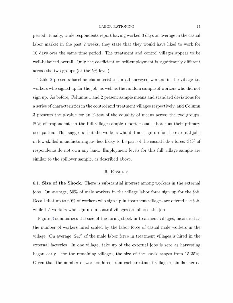
Figure 3 summarizes the size of the hiring shock in treatment villages, measured as

the number of workers hired scaled by the labor force of casual male workers in the

village. On average, 24% of the male labor force in treatment villages is hired in the

external factories. In one village, take up of the external jobs is zero as harvesting

began early. For the remaining villages, the size of the shock ranges from 15-35%.

Given that the number of workers hired from each treatment village is similar across

LABOR RATIONING 18

experimental rounds, the variation in shock size is driven primarily by variation in the

size of the male labor force across villages. Further, the hiring shock is slightly smaller

in peak months relative to lean months, though this difference is not significant.

6.2. Wages. We study the average impact of the hiring shock on local wages sepa-

rately for lean and peak months. For all worker-days in the recall period where the

worker reports hired employment for a daily wage, we construct two wage measures:

(i) cash wages; and (ii) total wages, which is the sum of cash wages and the monetary

value of all in-kind wages (e.g. tea, lunch etc.). Figure 5 compares the distributions of

total wages for treatment and control villages, limiting the sample to lean season ob-

servations (panel A) and to peak season observations (panel B). We cannot reject that

the wage distributions in treatment and control villages are equal in the lean months

(p-value from a Kolmogorov-Smirnov test is 0.196). In contrast, the wage distribution

for treatment villages is shifted to the right relative to the control villages in the peak

months (p-value < 0.001), indicating a rise in equilibrium wages.10

Estimates of Equations 1 and 2 on wages for the spillover sample are presented in the

first three columns of Table 3. Consistent with Prediction L1, we find no evidence that

wages in the village change in response to an external hiring shock in lean months (p-

value 0.456). However, in peak months, the hiring shock raises local wages by 0.0545

log points (p-value 0.0179) on average, consistent with Prediction P1. Estimates of

Equation 2 on the full village labor force (i.e. workers who signed up and workers

who did not sign up for the external jobs) are presented in Column 4. The predictions

hold with the full village sample as well — we find no detectable change in wages in

treatment villages in lean months, and an increase in equilibrium wages in treatment

villages in peak months.10Appendix Figure 1 compares the distribution of cash wages for treatment and control villages,limiting the sample to lean season observations (panel A) and to peak season observations (panel B).

LABOR RATIONING 19

6.3. Individual-Level Employment Spillovers. Next, we examine the spillover ef-

fects of the hiring shock on employment for individuals remaining in the village. For

all worker-days in the recall period, we construct two employment measures: (i) hired

employment in the casual labor market (agriculture or non-agriculture); and (ii) hired

employment in the casual labor market for a wage.

Estimates of Equations 1 and 2 on employment for the spillover sample are presented

in Table 4. Consistent with Prediction L2, we find positive employment spillover effects

in response to an external hiring shock in lean months. Specifically, the likelihood of

hired wage employment increases by 0.0552 percentage points (p-value 0.004) on a base

rate of wage employment of 0.145, which implies a 38% increase in employment among

workers who remain in the village. This is consistent with our prediction that workers

who were previously rationed fill in job slots when their peers are “removed” from the

labor market. In contrast, we cannot reject that there are no employment spillovers

onto the remaining workers in the peak months (p-value 0.400).

In Appendix Table 1, we present results on wages and employment using an alternate

specification. Instead of using a binary peak indicator, we interact the hiring shock with

a continuous measure for labor market demand — the (standardized) employment rate,

as measured in control villages for each experimental round. Our results are robust to

this alternate specification — for every one standard deviation increase in the village

employment rate, the hiring shock raises local wages by 0.0242 log points and reduces

hired wage employment by 0.0378 percentage points, on average.

6.4. Aggregate Employment and Crowd-Out. Finally, we study the average im-

pact of the hiring shock on aggregate employment levels in the village. To do this,

we examine the effects of the shock on hired wage employment (excluding the exter-

nal jobs generated at the factories) for two groups: (i) all workers who signed up for

the external jobs; and (ii) all workers in the village labor market — this consists of

LABOR RATIONING 20

those who signed up for the external jobs, as well as those who did not. Estimates of

Equation 2 on employment for these two groups are presented in Table 5.

Consistent with Prediction L3, there is no significant change in local aggregate em-

ployment in response to an external hiring shock in lean months (p-value 0.377). This

follows directly from the results above — since wages and local labor demand remain

unchanged, rationed workers fill up the job slots, leading to the same level of aggregate

employment. In contrast, consistent with Prediction P2, an external hiring shock leads

to a decline in aggregate employment in peak months. Employment for workers in

villages that experienced hiring shocks decreases by 0.040 percentage points (p-value

0.002) on a base rate of wage employment of 0.198, which implies a 20% decline in

aggregate employment in the village.

In Appendix Table 2, we run village-day level regressions using the hiring shock

as an instrument for employment in the external factories. Column 1 presents the

reduced-form result of the hiring shock on village employment, constructed by adding

up individual employment across all workers in the village. Consistent with the worker-

day level regression results in Table 5, we find no change in local aggregate employment

in response to the hiring shock in lean months (p-value 0.488), and a significant decline

in peak months (p-value 0.0895). The IV estimates in Column 3 suggest that every

day of work that is created in the external factories crowds out 0.149 days of private

labor market employment (p-value = 0.0659) in the peak months. In contrast, the

estimate for lean months is imprecisely estimated (p-value = 0.475), which implies

that generating jobs for up to 35% of workers in the village generates no crowd-out in

the private labor market in the lean season.

6.5. Elasticities. One concern is that we might be underpowered to detect wage in-

creases in the lean season. To rule this out, we compute the implied labor supply

elasticity from our wage and employment spillover results in the lean months. We take

the right hand side of the 95% confidence interval of the wage point estimate, 0.023,

LABOR RATIONING 21

and the 95% confidence interval of the employment spillover results in the lean sea-

son [.019, 0.092], which corresponds to a percentage increase of [12.9%, 63.0%]. The

labor supply elasticity required to induce this employment response for the individual

worker remaining in village is in the range of 5.6 - 27.4 — this is implausibly high,

and is substantively larger than the labor supply elasticity estimates derived by Breza

et al. (2019) among casual daily wage workers in the same setting.

6.6. Decomposing Rationing. We decompose rationing into involuntary unemploy-

ment and disguised unemployment (self-employed workers who would prefer wage la-

bor) by first testing the extent to which the hiring shock induces workers to prefer

wage employment over self-employment. We construct three self-employment mea-

sures: (i) total self-employment; (ii) self-employment in non-agriculture; and (iii) self-

employment in agriculture. Estimates of Equations 1 and 2 on self-employment in the

spillover sample are presented in Table 6. The external hiring shock leads to a 0.0390

percentage points decline in total self-employment in lean months, on a base of 0.13

(p-value 0.031). Workers thus reveal themselves as “forced entrepreneurs” by switching

from self-employment to wage employment when jobs are more easily available in their

village. Note that this reduction in self-employment accounts for an estimated 71% of

the employment spillovers.

We next examine the effect of a hiring shock on an indicator for any work activity

on that day in Column 1 of Table 7. We find no change in the overall reported

work status as a result of the hiring shocks in lean months. This is consistent with

disguised unemployment — workers who are rationed out of the wage labor market

remain engaged in some form of work activity, such that differences in work status

across treatment and control villages as a result of the hiring shocks in lean months

appear insignificant.

Further, we examine two sets of self-reported measures of involuntary unemployment

in Columns 2 and 3 of Table 7. The first is the traditional measure used in surveys,

LABOR RATIONING 22

which lists “would have liked to work but was unable to find any” as one of the options

for the activity for that day, along with hired employment or self-employment. The

second is an alternate measure that we propose, which asks workers to state whether

they would have accepted a job at the prevailing wage that day over whatever else

they had been doing (e.g., even if they were self-employed). If there is disguised

unemployment, then the first measure may understate rationing, because it will be

chosen only when the worker has reported no other activity.

Under the traditional measure (Column 2), we fail to find significant changes in

involuntary unemployment as a result of the hiring shocks in lean months. This is

unsurprising given the prevalence of disguised unemployment in this setting — workers

who appear gainfully employed in self-employment are involuntarily rationed out of the

wage labor market. Under the proposed alternate measure (Column 3), we find a 0.0553

percentage points (p-value 0.045) decline in involuntary unemployment as a result of

the hiring shocks in lean months. This decline corresponds closely to our spillover

effects in Table 4, suggesting that this alternate measure approximates the magnitude

of the revealed preference response.

7. Threats to Validity

There are several potential confounds that could give rise to (a subset of) predictions

L1-L3 even if there is no rationing.

Perfectly elastic labor supply. If labor supply is perfectly elastic at the prevailing

wage, this could generate our predictions in the absence of rationing. This alternate

explanation would require that no workers are willing to accept employment at a wage

below the prevailing wage. Figure 6 summarizes results from a labor supply elasticity

estimation exercise which was conducted in similar villages in the same districts as our

experimental sample. In this exercise, Breza et al. (2019) partner with agricultural

employers in the villages to randomize individual wage offers to workers in the local

LABOR RATIONING 23

labor market. When an employer offers a job to workers in his village at the prevailing

wage, 26% of otherwise unemployed workers accept the job. At a 10% wage cut, this

number drops to 18% – still well above zero. This suggests that labor supply in this

setting is far from perfectly elastic.

Wealth effects. The external jobs created under the hiring shocks generate an infusion

of wealth in treatment villages. A potential concern is that this may subsequently lead

to an expansion of local labor demand, which could counteract the supply shift and

subsequently generate no change in aggregate employment (Prediction L3). However, if

this alternate explanation is true, this should put even more upward pressure on wages,

which would be inconsistent with Prediction L1. We survey workers two weeks after the

hiring shock ends, when all workers are back in the village. With a demand expansion

from wealth infusion, we should expect to find continued employment increase. Under

rationing, however, the village should return to the way it was prior to the transient

hiring shock.

Estimates of Equation 2 on hired wage employment and self-employment for the

spillover sample two weeks after the shock ends are presented in Table 8. We find

no significant change in hired wage employment across treatment and control villages

in the lean months, two weeks after the hiring shock ends. In contrast, we do find

evidence for sustained decreased employment in treatment villages in the peak months,

consistent with a ratcheting effect. We also find possible sustained decreases in self-

employment, which allows us to rule out inter-temporal substitution in own farm work.

Change in composition of workers. While a substantial share of workers in the village

sign up for the external factory jobs, there may be some selection into this group. Note

that our design allows for workers in the village to be heterogeneous in ability, and for

some workers to be unqualified to work at the market wage rate. We also do not take

a stance on the underlying labor allocation mechanism in the presence of rationing, for

example, the most productive workers in the village are hired first.

LABOR RATIONING 24

One potential concern is that the quality of workers that are left behind in treatment

villages is on average lower than in control villages. If this puts downward pressure on

the wage, it could counteract the upward wage pressure from the supply shift, generat-

ing no change on average (Prediction L1). However, for this alternate explanation to

also generate Prediction L3, the demand elasticity for these workers would need to be

such that employers would still want to hire the exact same number of these workers

at w. Further, even if the average quality of workers that are left behind does decline,

our estimates would provide a lower bound for the level of rationing. By revealed pref-

erence, any worker that receives employment spillovers from the hiring shock must be

sufficiently productive to be employed at the market wage rate.

8. Conclusion

Our estimates of rationing are specific to labor markets in rural Odisha, India, dur-

ing lean months. Since there may be full employment during peak months, we cannot

conclude that rationed workers can be completely removed from villages without any

decline in agricultural productivity. Our results thus support the idea of “under-utilized

labor” but are inconclusive on whether there is “surplus labor” (Lewis, 1954; Leiben-

stein, 1957).

The prevalence of rationing suggests that there are lean periods in the year where

workers are not on their labor supply curve, and subsequently, wages do not play an

allocative role. This has important implications for analyses of labor market policies —

for example, in the estimation of general equilibrium effects of India’s national workfare

program, the National Rural Employment Guarantee Scheme (NREGS), that typically

provides rural workers with employment during the agricultural lean season. The role

of seasonality should therefore be taken seriously as an input in labor market analysis,

and subsequently, in the formulation of policies.

LABOR RATIONING 25

Finally, while the magnitudes of our estimates are only relevant for our study context,

the measurement problem of involuntary un-and under-employment and the revealed

preference methodology we employ have much broader relevance in both poor and

rich countries. We find that two different labor market paradigms are relevant in the

Odisha context, depending on predictable fluctuations in labor market slack. This

implies that the labor market can be fundamentally different in its functioning over

the course of the year. Finding evidence for rationing in our context suggests taking

seriously the idea that labor markets may not clear in other rural, developing country

settings where employment rates are low for some parts of the year. This provides

impetus and direction for expanded work on labor market frictions in poor countries.

References

Akram, A. A., S. Chowdhury, and A. M. Mobarak (2017): “Effects of emigra-

tion on rural labor markets,” Tech. rep., National Bureau of Economic Research.

Benjamin, D. (1992): “Household composition, labor markets, and labor demand:

Testing for separation in agricultural household models,” Econometrica: Journal of

the Econometric Society, 287–322.

Bowers, N. and F. W. Horvath (1984): “Keeping time: An analysis of errors

in the measurement of unemployment duration,” Journal of Business & Economic

Statistics, 2, 140–149.

Breza, E., S. Kaur, and N. Krishnaswamy (2019): “Scabs: The Social Suppres-

sion of Labor Supply,” Tech. rep., National Bureau of Economic Research.

Breza, E., S. Kaur, and Y. Shamdasani (2018): “The morale effects of pay

inequality,” The Quarterly Journal of Economics, 133, 611–663.

Breza, E. and C. Kinnan (2018): “Measuring the equilibrium impacts of credit:

Evidence from the Indian microfinance crisis,” Working Paper.

LABOR RATIONING 26

Card, D., A. Mas, E. Moretti, and E. Saez (2012): “Inequality at work: The

effect of peer salaries on job satisfaction,” The American Economic Review, 102,

2981–3003.

Crepon, B., E. Duflo, M. Gurgand, R. Rathelot, and P. Zamora (2013):

“Do labor market policies have displacement effects? Evidence from a clustered

randomized experiment,” The Quarterly Journal of Economics, 128, 531–580.

Donaldson, D. and D. Keniston (2016): “Dynamics of a Malthusian Economy:

India in the Aftermath of the 1918 Influenza,” Working Paper.

Eckaus, R. S. (1955): “The factor proportions problem in underdeveloped areas,”

American Economic Review, 539–565.

Fellner, W. (1976): “Towards a Reconstruction of Macroeconomics,” Tech. rep.,

American Enterprise Institute.

Ham, J. C. (1982): “Estimation of a labour supply model with censoring due to

unemployment and underemployment,” The Review of Economic Studies, 49, 335–

354.

Imbert, C. and J. Papp (2015): “Labor market effects of social programs: Evi-

dence from India’s employment guarantee,” American Economic Journal: Applied

Economics, 7, 233–263.

Jayachandran, S. (2006): “Selling labor low: Wage responses to productivity shocks

in developing countries,” Journal of Political Economy, 114, 538–575.

Kaur, S., S. Mullainathan, S. Oh, and F. Schilbach (2019): “Does Financial

Strain Lower Productivity?” Working Paper.

Leibenstein, H. (1957): Economic backwardness and economic growth : Studies in

the theory of economic development., New York: Wiley.

Lewis, W. A. (1954): “Economic Development With Unlimited Supplies of Labour,”

The Manchester School, 22, 139–191.

LABOR RATIONING 27

Mathiowetz, N. A. and G. J. Ouncan (1988): “Out of work, out of mind: Re-

sponse errors in retrospective reports of unemployment,” Journal of Business &

Economic Statistics, 6, 221–229.

Muralidharan, K., P. Niehaus, and S. Sukhtankar (2017): “General equi-

librium effects of (improving) public employment programs: Experimental evidence

from india,” Tech. rep., National Bureau of Economic Research.

Rosenzweig, M. R. (1988): “Labor markets in low-income countries,” in Handbook

of Development Economics, Elsevier, vol. 1, 713–762.

Singh, I., L. Squire, J. Strauss, et al. (1986): Agricultural household models:

Extensions, applications, and policy., Johns Hopkins University Press.

Taylor, J. (2008): “Involuntary unemployment,” The New Palgrave Dictionary of

Economics, Second Edition.

LABOR RATIONING 28

Figures

01

23

Den

sity

0 .2 .4 .6 .8Average daily employment rate per village

(a) Wage + Self Employment

01

23

45

Den

sity

0 .1 .2 .3 .4Average daily employment rate per village

(b) Wage Employment Only

Figure 1. Distribution of Employment Rates

Note: Figure shows average village-level daily wage and self-employmentrates in panel A, and average village-level daily wage employment ratesonly in panel B, using responses from the employment recall grid. Onlycontrol villages are included.

LABOR RATIONING 29

Wage

Village Empl.E

w

S ′(treatment)

S

D

E ′

w′

text to align

(a) H0 : No Rationing (ED ≥ ES)

Wage

Village Empl.

S

S ′(treatment)

D

E = ED ESE′S

w

Rationing

(b) H1 : Rationing (ED < ES)

Figure 2. Effects of a Negative Labor Supply Shock

Note: Figure shows the effects of a negative supply shock on employmentand wages under market clearing (ED ≥ ES) in panel A, and underrationing (ED < ES) in panel B.

0.0

5.1

.15

.2Fr

actio

n

0 .1 .2 .3 .4Fraction of male labor force

Figure 3. Size of the Experimental Hiring Shock

Note: Figure shows the size of the experimental hiring shock in treatmentvillages. This is measured as number of workers hired scaled by the sizeof the male labor force in the village. Mean = 0.24.

LABOR RATIONING 30

(a) No hiring shock (b) Hiring shock

Figure 4. Analysis Samples

Note: Figure summarizes the analysis sample in control villages in panelA, and treatment villages in panel B. The grey shaded areas denoteworkers who signed up but were not offered employment at the externalfactories — this constitutes the spillover sample.

0.2

.4.6

.81

Den

sity

0 100 200 300 400 500Daily wage (total)

Control villages Treatment villages

(a) Lean Season

0.2

.4.6

.81

Den

sity

0 100 200 300 400 500Daily wage (total)

Control villages Treatment villages

(b) Peak Season

Figure 5. Wage Level Effects (Cash + In-Kind Wages)

Note: Figure compares the distribution of total wages for treatment andcontrol villages, limiting the sample to lean season observations only inpanel A, and peak season observations only in panel B. The p-value forthe equality of distributions from a Kolmogorov-Smirnov test is 0.196(panel A), and <0.001 (panel B).

LABOR RATIONING 31

0

0.1

0.2

0.3

0.4

10% below prevailing wage Prevailing wage

Figure 6. Job take-up: private wage offers

Note: Figure illustrates take up of a job offer at different wage ratesamong casual workers in villages similar to our study sample, in thesame districts of Odisha, India. This data comes from a labor supplyestimation exercise conducted by Breza et al. (2019).

LAB

OR

RAT

ION

ING

32

Tables

Table 1. Baseline Characteristics of Spillover Sample

(1) (2) (3)No hiring shock Hiring shock P-value of diff.

Occupation: Laborer 0.963 0.973 0.494(0.189) (0.163)

Landless 0.377 0.359 0.596(0.485) (0.481)

Hired employment 0.222 0.230 0.769(0.319) (0.340)

Hired wage employment 0.177 0.182 0.811(0.288) (0.308)

Log wage (total) 5.487 5.539 0.267(0.386) (0.354)

Self employment 0.115 0.077 0.029∗∗(0.244) (0.193)

Days worked in casual labor market (in past 14 days) 3.033 3.024 0.973(3.438) (3.087)

Days would have liked to work in casual labor market (in past 14 days) 9.841 10.150 0.261(3.402) (3.282)

Notes: We restrict to the spillover sample (workers who signed up for external jobs but were not offered employment).Cols 1 and 2 presents baseline means and standard deviations of characteristics for workers in control and treatmentvillages respectively. Col 3 presents p-values from an F-test of the equality of means across the treatment and controlvillages. Observations are at the worker level. N=1048

LAB

OR

RAT

ION

ING

33

Table 2. Baseline Characteristics of Full Village Sample

(1) (2) (3)No hiring shock Hiring shock P-value of diff.

Occupation: Laborer 0.891 0.891 0.997(0.311) (0.311)

Landless 0.352 0.332 0.405(0.478) (0.471)

Hired employment 0.198 0.225 0.058∗(0.303) (0.317)

Hired wage employment 0.156 0.167 0.355(0.270) (0.278)

Log wage (total) 5.518 5.557 0.370(0.426) (0.508)

Self employment 0.126 0.110 0.263(0.262) (0.246)

Days worked in casual labor market (in past 14 days) 2.771 2.620 0.424(3.346) (3.325)

Days would have liked to work in casual labor market (in past 14 days) 8.839 8.226 0.018∗∗(4.252) (4.608)

Notes: We restrict to the full village sample. Cols 1 and 2 presents baseline means and standard deviations of character-istics for workers in control and treatment villages respectively. Col 3 presents p-values from an F-test of the equality ofmeans across the treatment and control villages. Observations are at the worker level. N=2511

LABOR RATIONING 34

Table 3. Wage Effects

(1) (2) (3) (4)Log cash wage Log total wage Log total wage Log total wage

Hiring shock -0.0203 -0.00907 -0.0141 0.00821(0.019) (0.020) (0.019) (0.031)

Hiring shock * Peak 0.0741** 0.0654** 0.0686** 0.0588(0.030) (0.031) (0.030) (0.036)

Sample Spillover Spillover Spillover Full VillageBaseline controls No No Yes YesTest: Shock + Shock*Peak 0.0230 0.0225 0.0179 0.000283Control mean: lean 5.445 5.494 5.494 5.498Control mean: peak 5.428 5.505 5.505 5.495N (worker-days) 1602 1603 1603 2805

Notes: Cols 1-3 restrict to the spillover sample (workers who signed up for external jobs butwere not offered employment). Col 4 includes all male workers in the village with appropriateweights. Total wage = cash + in-kind wages. Controls include worker-level mean employmentand wage levels at baseline. Regressions include round (strata) FEs. Standard errors clusteredat the village level in parentheses.

Table 4. Employment Spillovers

(1) (2) (3)Hired employment Hired wage employment Hired wage employment

Hiring shock 0.0600*** 0.0598*** 0.0552***(0.019) (0.020) (0.018)

Hiring shock * Peak -0.0611** -0.0676** -0.0745**(0.030) (0.032) (0.029)

Baseline controls No No YesTest: Shock + Shock*Peak 0.961 0.762 0.400Control mean: lean 0.154 0.145 0.145Control mean: peak 0.264 0.213 0.213N (worker-days) 9466 9466 9459

Notes: Cols 1-3 restrict to the spillover sample (workers who signed up for external jobs but werenot offered employment). Hired employment = 1{worker hired that day}, and hired wage employ-ment = 1{worker hired that day and paid a wage}. Controls include worker-level mean employmentand wage levels at baseline. Regressions include round (strata) FEs. Standard errors clustered atthe village level in parentheses.

LABOR RATIONING 35

Table 5. Aggregate Employment

(1) (2) (3)Hired wage employment Hired wage employment Hired wage employment

Hiring shock 0.0552*** -0.0109 0.0173(0.018) (0.014) (0.019)

Hiring shock * Peak -0.0745** -0.0528** -0.0574**(0.029) (0.021) (0.024)

Sample Spillover Full Labor Force Full VillageBaseline controls Yes Yes YesTest: Shock + Shock*Peak 0.400 0.0000809 0.00215Control mean: lean 0.145 0.127 0.131Control mean: peak 0.213 0.199 0.198R-squared 0.116 0.104 0.101N (worker-days) 9459 17716 22384

Notes: Col 1 restricts to only the spillover sample as a reference. Col 2 include all male workers in thevillage who signed up for the experimental job with appropriate weights. Col 3 includes all male workersin the village with appropriate weights. Hired wage employment = 1{worker hired that day and paid awage}. Controls include worker-level mean employment and wage levels at baseline. Regressions includeround (strata) FE. Standard errors clustered at the village level in parentheses.

Table 6. Self-Employment

(1) (2) (3) (4)Self employment Self employment Self empl: non-agri Self empl: agri

Hiring shock -0.0390** -0.0332* -0.0122** -0.0265(0.018) (0.018) (0.005) (0.019)

Hiring shock * Peak 0.0151 0.00884 -0.00901 0.0267(0.025) (0.025) (0.010) (0.024)

Baseline controls No Yes Yes YesTest: Shock + Shock*Peak 0.186 0.171 0.0333 0.990Control mean: lean 0.130 0.130 0.0236 0.107Control mean: peak 0.104 0.104 0.0247 0.0794N (worker-days) 9466 9459 9459 9459

Notes: Cols 1-4 restrict to the spillover sample (workers who signed up for external jobs but were notoffered employment). Each dependent variable is a binary indicator for whether worker reported eachstated activity that day. Controls include worker-level mean employment and wage levels at baseline.Regressions include round (strata) FE. Standard errors clustered at the village level in parentheses.

LABOR RATIONING 36

Table 7. Measuring Involuntary Unemployment

(1) (2) (3)Any work Invol unempl: trad Invol unempl: alt

Hiring shock 0.00705 -0.0230 -0.0553**(0.023) (0.030) (0.027)

Hiring shock * Peak -0.0234 0.0311 0.0622(0.028) (0.040) (0.039)

Baseline controls Yes Yes YesTest: Shock + Shock*Peak 0.326 0.752 0.804Control mean: lean 0.340 0.491 0.588Control mean: peak 0.394 0.401 0.548N (worker-days) 9459 9459 9459

Notes: Cols 1-4 restrict to the spillover sample (workers who signed up for ex-ternal jobs but were not offered employment). Any work = 1{worker reportsany work that day}. The dependent variable in Column 2 is a binary indicatorfor whether worker reported “would have liked to work but was unable to findany” as his activity status for that day. The dependent variable in Column 3is a binary indicator for whether worker stated that they would have accepteda job at the prevailing wage that day over whatever else they had been doing.Controls include worker-level mean employment and wage levels at baseline.Regressions include round (strata) FE. Standard errors clustered at the villagelevel in parentheses.

Table 8. Impacts 2 Weeks After End of Hiring Shock

(1) (2)Hired wage employment Self employment

Hiring shock 0.00762 -0.0212(0.025) (0.019)

Hiring shock * Peak -0.0495 -0.0140(0.033) (0.027)

Baseline controls Yes YesTest: Shock + Shock*Peak 0.0444 0.0695Control mean: lean 0.172 0.170Control mean: peak 0.210 0.138N (worker-days) 7916 7916

Notes: Cols 1 and 2 restrict to the spillover sample (workers who signedup for external jobs but were not offered employment). Controls includeworker-level mean employment and wage levels at baseline. Regressionsinclude round (strata) FE. Standard errors clustered at the village levelin parentheses.

LABOR RATIONING 37

Appendix A. Appendix Figures

0.2

.4.6

.81

Den

sity

0 100 200 300 400 500Daily wage (cash)

Control villages Treatment villages

(a) Lean Season

0.2

.4.6

.81

Den

sity

0 100 200 300 400 500Daily wage (cash)

Control villages Treatment villages

(b) Peak Season

Figure 1. Wage Level Effects (Cash Wages)

Note: Figure compares the distribution of cash wages for treatment andcontrol villages, limiting the sample to lean season observations in panelA, and to peak season observations in panel B. The p-value for the equal-ity of distributions from a Kolmogorov-Smirnov test is 0.222 (panel A)and <0.001 (panel B).

LABOR RATIONING 38

Appendix B. Appendix Tables

Table 1. Treatment Effects: Continuous Peak Specification

(1) (2)Log total wage Hired wage employment

Hiring shock -0.0595 0.144***(0.0550) (0.0469)

Hiring shock x Empl rate (sd) 0.0242* -0.0378***(0.0139) (0.0137)

Baseline controls Yes YesControl mean: lean 5.494 0.145Control mean: peak 5.505 0.213N (worker-days) 1603 9466

Notes: Cols 1 and 2 restrict to the spillover sample (workers who signedup for external jobs but were not offered employment). Controls includeworker-level mean employment and wage levels at baseline. Regressionsinclude round (strata) FEs. Standard errors clustered at the village levelin parentheses.

Table 2. Aggregate Employment Effects and Crowd-Out

(1) (2) (3)Hired wage empl Hiring shock empl Hired wage empl

Hiring shock 0.0174 0.190***(0.025) (0.009)

Hiring shock * Peak -0.0463* 0.00179(0.027) (0.016)

Hiring shock empl 0.0923(0.129)

Hiring shock empl * Peak -0.242*(0.136)

Specification RF FS IVBaseline controls Yes Yes YesTest: Shock + Shock*Peak 0.0895 1.36e-19 0.0659N (village-days) 788 788 788

Notes: Cols 1-3 include all male workers in the village with appropriate weights. Con-trols include mean employment and wages at the village-day level at baseline. Re-gressions include round (strata) FEs. Standard errors clustered at the village level inparentheses.