Laboratory Assignment 2 Signal Sampling, Manipulation, and Playback

PURPOSE This lab will introduce you to the laboratory equipment and the software that allows you to link your computer to the hardware. Specifically, you will learn how to use the equipment in the laboratory to convert analog signals (e.g., from a microphone or function generator) into digital signals that can be displayed and/or modified using MATLAB. You will learn how to perform mathematical modifications to digital audio signals in order to produce some interesting audio effects. In the process, you will learn how to take the original or modified digital signals and convert them to analog signals for display on an oscilloscope or for audio playback. In this text, we refer to .wav files for convenience. Substitute whatever file type is necessary for your system, as discussed in the Foreword. Also, see Appendix A for a full description of the sound file conversion program.

2.1 OBJECTIVES By the end of this assignment, you should be able to: 1. Use the laboratory setup to import real signals from a microphone or function generator into the computer and to export signals to an output device, such as headphones or an oscilloscope. 2. Use some simple mathematical manipulations to alter audio properties of signals.

2.2 REFERENCE Review Topics 1. Mathematical representations of continuous- and discrete-time signals 2. Mathematical operations on signals 3. Representation of sinusoids at specified frequencies Exploratory Topics 1. Sampling, quantization, and A/D conversion 2. Digital audio signal manipulation using MATLAB 3. Laboratory audio platform capabilities and requirements

2.3 LABORATORY PREPARATION Question 1. In this lab, you will sample a 100-Hz tone at 8000 samples per second. If samples of this signal are stored as a row vector, what will be the effect of your MATLAB function file half on the pitch and duration of the tone if the playback rate is identical to the sampling rate? Similarly, what will be the effect of double? Be specific; indicate pitch in Hertz and duration in seconds relative to the original signal. Use sketches to help explain your answers. How can you use your functions half and double if the original sampled signal is stored as a column vector? Question 2. In this lab you will apply the MATLAB functions fliplr and flipud to a sampled segment of your speech. Use the MATLAB help function to find out what these commands do. For each function, explain the impact it will have on both row and column vectors. What will you expect to hear when you play back the signal returned by these functions, assuming that you use the original sampling rate and the signal is stored as a column vector? Question 3. Given a sampled signal contained in the vector x in MATLAB, write a MATLAB function to generate a vector that includes the original signal plus an echo occurring T seconds after the start of the original signal and having amplitude that is a times as large as that of the original signal. Use vector operations to avoid time-consuming loops.

2.4 BACKGROUND In order to store, display, and modify audio signals on a digital computer, the physical analog signals must be digitized. This is done through two processes known as sampling and quantization, collectively referred to as analog-to-digital (A/D) conversion by convention. Here we provide a brief review of sampling using only time domain concepts; in a later chapter, we will revisit sampling and develop more analytical insight using frequency-domain concepts. Sampling Review Consider an analog signal x(t) that can be viewed as a continuous function of time, as shown in Figure 2.4.1 (a). We can represent this signal as a discrete-time signal by using values of x(t) at intervals of nTs to form x[n], as shown in Figure 2.4.1(b). Essentially, we are “picking points off of the graph” of x(t) at regular intervals. Mathematically, we write

snTttxnx

== )(][ where Ts is called the sampling period.

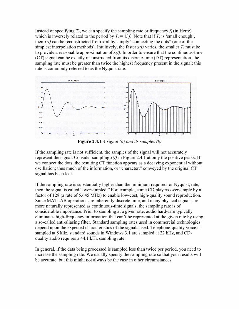
Instead of specifying Ts, we can specify the sampling rate or frequency fs (in Hertz) which is inversely related to the period by Ts = 1/ fs. Note that if Ts is ‘small enough’, then x(t) can be reconstructed from xml by simply “connecting the dots” (one of the simplest interpolation methods). Intuitively, the faster x(t) varies, the smaller Ts must be to provide a reasonable approximation of x(t). In order to ensure that the continuous-time (CT) signal can be exactly reconstructed from its discrete-time (DT) representation, the sampling rate must be greater than twice the highest frequency present in the signal; this rate is commonly referred to as the Nyquist rate.

Figure 2.4.1 A signal (a) and its samples (b)

If the sampling rate is not sufficient, the samples of the signal will not accurately represent the signal. Consider sampling x(t) in Figure 2.4.1 at only the positive peaks. If we connect the dots, the resulting CT function appears as a decaying exponential without oscillation; thus much of the information, or “character,” conveyed by the original CT signal has been lost. If the sampling rate is substantially higher than the minimum required, or Nyquist, rate, then the signal is called “oversampled.” For example, some CD players oversample by a factor of 128 (a rate of 5.645 MHz) to enable low-cost, high-quality sound reproduction. Since MATLAB operations are inherently discrete time, and many physical signals are more naturally represented as continuous-time signals, the sampling rate is of considerable importance. Prior to sampling at a given rate, audio hardware typically eliminates high-frequency information that can’t be represented at the given rate by using a so-called anti-aliasing filter. Standard sampling rates used in commercial technologies depend upon the expected characteristics of the signals used. Telephone-quality voice is sampled at 8 kllz, standard sounds in Windows 3.1 are sampled at 22 kHz, and CD-quality audio requires a 44.1 kHz sampling rate. In general, if the data being processed is sampled less than twice per period, you need to increase the sampling rate. We usually specify the sampling rate so that your results will be accurate, but this might not always be the case in other circumstances.

Quantization Quantization is the process by which signal sample values are represented as binary digits to permit manipulation on a digital computer. The number of bits used to define a sample indicates how many different analog levels can be represented. For example, using 8 bits per sample permits representation of up to 256 different levels, whereas 16-bit sampling can represent 65536 levels. The maximum difference between adjacent sampling levels determines how accurately the amplitude of the digitally represented samples approximates the sample values obtained from the original continuous-time signal. The more sampling levels there are the more accurate the representation. One commonly used measure of quantization accuracy is the signal-to-noise ratio (SNR) which is the ratio of the amount of power in the signal to that in the “noise” introduced by quantization errors. Larger values of SNR indicate higher-quality signals. For a full-range signal (meaning that representing the full range of signal values in the original signal requires using all possible discrete amplitude levels), the SNR can be roughly calculated as (6n - 7.2) dB, where n is the number of bits. Using this formula, 16-bit sampling has a SNR of —89 dB while 8-bit sampling has an SNR of -41 dB. If the signal ranged from -1 V to + 1 V, the quantization error for 16-bit sampling would be +1- 30 µV. In essence, the quantization process introduces controlled errors so that we can use a computer to process the signals. Why would we deliberately introduce noise into a signal rather than simply using continuous-time, analog processing? There are many advantages, but the two major ones are that (1) typically, more sophisticated mathematical operations for signal processing, communication and control systems can be performed using a computer, and (2) it is much easier to reduce errors, caused by disturbances during transmission or degradation due to heat or aging, if the information is stored in a binary format: recovering the information requires only a choice between a binary one and zero, and codes can be used to help detect and correct errors. By introducing controlled error into the signal, we can prevent corruption from uncontrolled noise sources. Loudness and Pitch in Audio Signals Since you are likely to be using audio signals in several laboratory assignments, we would like to comment briefly at this point on how perceived loudness relates to signal amplitude, and how perceived changes in pitch relate to changes in frequency. These ideas will continue to be reinforced as you proceed through the laboratory assignments. First, linear changes in perceived loudness correspond to exponential changes in signal amplitude since the loudness depends upon the signal power. For a simple tone (sinusoid) at 100 Hz, the average power over a single period is defined as

∫ =⎟⎟⎠⎞

⎜⎜⎝⎛

⎟⎠⎞⎜

⎝⎛=

T

AdttT

AT

erAveragePow2

2sin1 22π

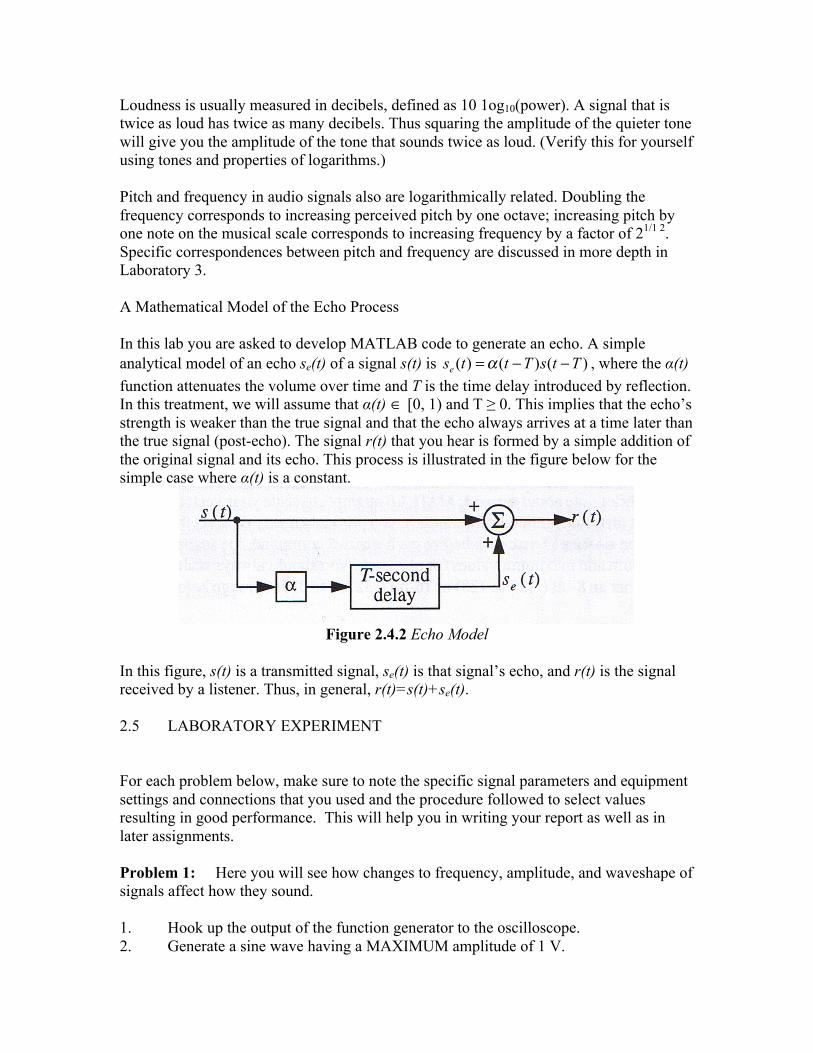
Loudness is usually measured in decibels, defined as 10 1og10(power). A signal that is twice as loud has twice as many decibels. Thus squaring the amplitude of the quieter tone will give you the amplitude of the tone that sounds twice as loud. (Verify this for yourself using tones and properties of logarithms.) Pitch and frequency in audio signals also are logarithmically related. Doubling the frequency corresponds to increasing perceived pitch by one octave; increasing pitch by one note on the musical scale corresponds to increasing frequency by a factor of 21/1 2. Specific correspondences between pitch and frequency are discussed in more depth in Laboratory 3. A Mathematical Model of the Echo Process In this lab you are asked to develop MATLAB code to generate an echo. A simple analytical model of an echo se(t) of a signal s(t) is )()()( TtsTttse −−=α , where the α(t) function attenuates the volume over time and T is the time delay introduced by reflection. In this treatment, we will assume that α(t) ∈ [0, 1) and T ≥ 0. This implies that the echo’s strength is weaker than the true signal and that the echo always arrives at a time later than the true signal (post-echo). The signal r(t) that you hear is formed by a simple addition of the original signal and its echo. This process is illustrated in the figure below for the simple case where α(t) is a constant.

Figure 2.4.2 Echo Model

In this figure, s(t) is a transmitted signal, se(t) is that signal’s echo, and r(t) is the signal received by a listener. Thus, in general, r(t)=s(t)+se(t). 2.5 LABORATORY EXPERIMENT For each problem below, make sure to note the specific signal parameters and equipment settings and connections that you used and the procedure followed to select values resulting in good performance. This will help you in writing your report as well as in later assignments. Problem 1: Here you will see how changes to frequency, amplitude, and waveshape of signals affect how they sound. 1. Hook up the output of the function generator to the oscilloscope. 2. Generate a sine wave having a MAXIMUM amplitude of 1 V.

3. Also connect the output from the function generator to the input (line in) of the sound card. 4. Connect the headphones to the appropriate sound card output. 5. Listen to the headphones and watch the oscilloscope as you vary the frequency, amplitude, and waveshape (square, triangular, sinusoidal). Notice how the audio properties of these signals differ. Document your observations regarding how the relative audio properties of the signal change as you vary the amplitude, frequency, and waveshape of the signal. Be specific. If you double the frequency, what happens to the pitch? If you decrease the amplitude to half of its original value, is the result halt as loud? How does the perceived audio character of the signal at a lixed frequency change with the changing waveshape? Problem 2: Playback of a Sampled Signal The file ‘P_2_1 .wav’ contains a segment of a sampled signal. Play this file using your computer’s sound programs, and play the same file using the sound command from inside of MATLAB. You will need to use wavread to load in the sound file. A brief note about sound: MATLAB attempts to scale your vector for playback. If you get distorted, unintelligible sounds, you probably need to correct the autoscaling. If you type saxis ( ‘auto’) before each sound command, the scaling will reset the minimum and maximum values for playback. You should always scale your vector to be in either an 8-bit (-127 to 128) or 16-bit (-32767 to 32768) range before storing as a sound file. What do you hear? Can you identify it? Comment on the quality. Problem 3: Sampling and Playback of Signals In this part of the experiment, you will learn how to digitize a signal and examine the resulting data with MATLAB. Be sure to save the signals that you sample in this section as vectors in MATLAB as you will use them in the next section. NOTE: Using short segments of digitized signals will allow you to proceed much more quickly in the lab. 1. Generate a 100-Hz sine wave with the function generator. A signal amplitude between 0.5 and 0.7 V is strongly recommended (verify with the oscilloscope before connecting input to the card!). 2. Use your computer’s sound software to sample the sine wave (a sampling frequency of 8000 Hz will be sufficient). 3. Play back your waveform and view it on the oscilloscope. 4. Use the wavread command from inside MATLAB to import your .wav file and make a plot of the signal. 5. Now repeat steps 2-4 except sample your own speech instead of the sine wave.

Generate plots of segments of your tone and speech signals Be sure to label your axes. Indicate how features on the plot correspond to sounds in your speech sample. Problem 4: Some Audio Effects Apply each of the following MATLAB functions to both the sine wave and speech segments that you digitized in the previous section. Store your new signal to a .wav file using ‘writewav’ and then play back the signal. Observe the effect of these digital manipulations on the audio properties of the signal. 1. The MATLAB function half created by you in the first laboratory. 2. The MATLAB function double created by you in the first laboratory. 3. The MATLAB functions fliplr and flipud . Document how the MATLAB functions you use change the properties of the original tone and speech signals. Compare and contrast the relative impact that these functions have on the audio properties of the speech and tone. Does the speech segment sound like it was produced by the same speaker as the original? Why or why not? Problem 5: Echo Effects Use the MATLAB function file you created to create an echo signal using your original speech signal and a constant attenuation. You will need to create a signal that is a scaled version of the original and add it to the original with the desired offset in time. Experiment with different values for the time delay and attenuation. Listen to the resulting signals and note your observations. 1. Generate a 0.25-second echo effect. Let α=0.65. 2. Use a non-constant attenuation function, such as an exponential: τα /)( tAet −= . Determine values of A and τ that make an interesting effect. 3. Use several different delays and amplitudes to get a variety of echoes. 4. Use an oscillatory attenuation function, such as ( )tAt ωα cos)( = . Describe the impact that your choice of time delay T and attenuation α have on the resulting synthesized echo. Be specific about changes in parameters and relative impact on sound. What happens if T changes during the echo-generation process?

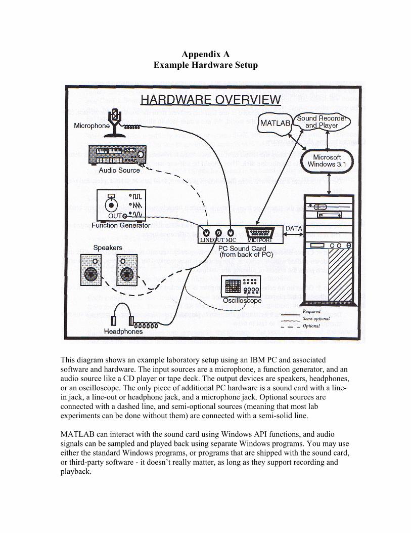
Appendix A Example Hardware Setup

This diagram shows an example laboratory setup using an IBM PC and associated software and hardware. The input sources are a microphone, a function generator, and an audio source like a CD player or tape deck. The output devices are speakers, headphones, or an oscilloscope. The only piece of additional PC hardware is a sound card with a line-in jack, a line-out or headphone jack, and a microphone jack. Optional sources are connected with a dashed line, and semi-optional sources (meaning that most lab experiments can be done without them) are connected with a semi-solid line. MATLAB can interact with the sound card using Windows API functions, and audio signals can be sampled and played back using separate Windows programs. You may use either the standard Windows programs, or programs that are shipped with the sound card, or third-party software - it doesn’t really matter, as long as they support recording and playback.