Laboratory DC Motor Position Modeling and Control in Simulinkinc.kmutt.ac.th/course/inc354/lead_lagv3.pdf · Laboratory DC Motor Position Modeling and Control in Simulink Objectives:

Laboratory

DC Motor Position Modeling and Control in Simulink

Objectives:At the end, student should

1. be able to construct linear and nonlinear models in Simulink;

2. understand a systematic procedure of designing a lead-lag compensator by using fre-quency response method;

1 IntroductionThis introduction is a preliminary material. Student must go through this section beforetake the Lab. Random selected questions will be asked each student one by one. Any groupwho has no idea about this introduction will be definitely sent back home.

1.1 Simulink

Simulink is the one of software packages for modeling, simulating, and analyzing dynamicalsystems based on Matlab. It supports linear and nonlinear systems, modeled in continuoustime, sampled time, or a hybrid of the two.

For modeling, Simulink provides a graphical user interface (GUI) for building models asblock diagrams, using click-and-drag mouse operations. With this interface, you can draw themodels just as you would with pencil and paper (or as most textbooks depict them). This is afar cry from previous simulation packages that require you to formulate differential equationsand difference equations in a language or program. Simulink includes a comprehensive blocklibrary of sinks, sources, linear and nonlinear components, and connectors.

After you define a model, you can simulate it, using a choice of integration methods, eitherfrom the Simulink menus or by entering commands in MATLAB’s command window. Themenus are particularly convenient for interactive work, while the command-line approach isvery useful for running a batch of simulations. Using scopes and other display blocks, youcan see the simulation results while the simulation is running. In addition, you can changeparameters and immediately see what happens, for “what if” exploration. The simulationresults can be put in the MATLAB workspace for postprocessing and visualization.

1.1.1 Simulink Basics Tutorial – Block Libraries

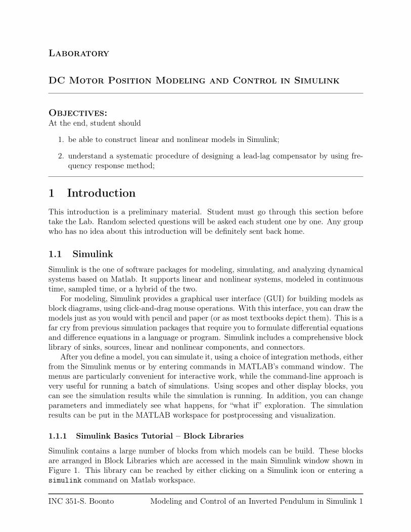
Simulink contains a large number of blocks from which models can be build. These blocksare arranged in Block Libraries which are accessed in the main Simulink window shown inFigure 1. This library can be reached by either clicking on a Simulink icon or entering asimulink command on Matlab workspace.

INC 351-S. Boonto Modeling and Control of an Inverted Pendulum in Simulink 1

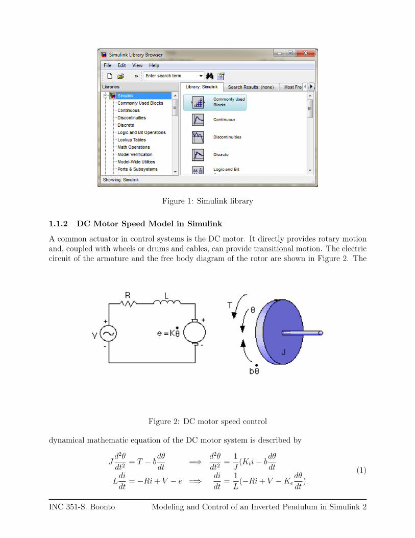
Figure 1: Simulink library

1.1.2 DC Motor Speed Model in Simulink

A common actuator in control systems is the DC motor. It directly provides rotary motionand, coupled with wheels or drums and cables, can provide transitional motion. The electriccircuit of the armature and the free body diagram of the rotor are shown in Figure 2. The

Figure 2: DC motor speed control

dynamical mathematic equation of the DC motor system is described by

Jd2θ

dt2= T − b

dθ

dt=⇒ d2θ

dt2=

1

J(Kti− b

dθ

dt

Ldi

dt= −Ri+ V − e =⇒ di

dt=

1

L(−Ri+ V −Ke

dθ

dt).

(1)


The model can be constructed in Simulink by the following step:

1. Insert two Gain blocks, (from the Simulink/Commonly Used Blocks) one attached toeach of the integrators.

2. Edit the gain block corresponding to angular acceleration by double-clicking it andchanging its value to 1/J .

3. Change the label of this Gain block to “inertia” by clicking on the word “Gain” under-neath the block.

4. Similarly, edit the other Gain’s value to “1/L” and it’s label to Inductance.

5. Insert two Sum blocks, one attached by a line to each of the Gain blocks.

6. Edit the signs of the Sum block corresponding to rotation to “+-” since one term ispositive and one is negative.

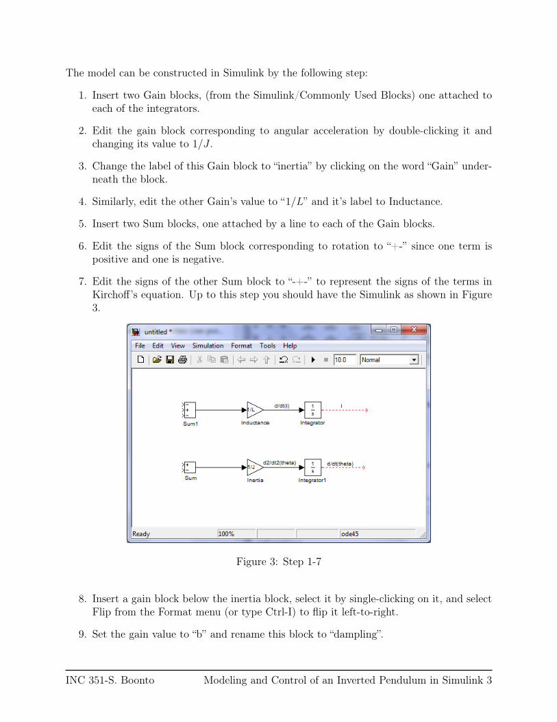
7. Edit the signs of the other Sum block to “-+-” to represent the signs of the terms inKirchoff’s equation. Up to this step you should have the Simulink as shown in Figure3.

Figure 3: Step 1-7

8. Insert a gain block below the inertia block, select it by single-clicking on it, and selectFlip from the Format menu (or type Ctrl-I) to flip it left-to-right.

9. Set the gain value to “b” and rename this block to “dampling”.


10. Tap a line off the rotational integrator’s output and connect it to the input of thedamping gain block.

11. Draw a line from the damping gain output to the negative input of the rotational Sumblock.

12. Insert a gain block attached to the positive input of the rotational Sum block with aline.

13. Edit it’s value to “K” to represent the motor constant and Label it “Kt”.

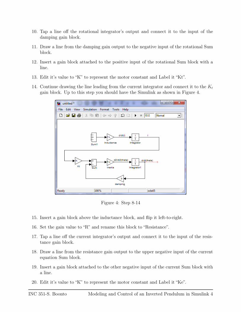
14. Continue drawing the line leading from the current integrator and connect it to the Kt

gain block. Up to this step you should have the Simulink as shown in Figure 4.

Figure 4: Step 8-14

15. Insert a gain block above the inductance block, and flip it left-to-right.

16. Set the gain value to “R” and rename this block to “Resistance”.

17. Tap a line off the current integrator’s output and connect it to the input of the resis-tance gain block.

18. Draw a line from the resistance gain output to the upper negative input of the currentequation Sum block.

19. Insert a gain block attached to the other negative input of the current Sum block witha line.

20. Edit it’s value to “K” to represent the motor constant and Label it “Ke”.


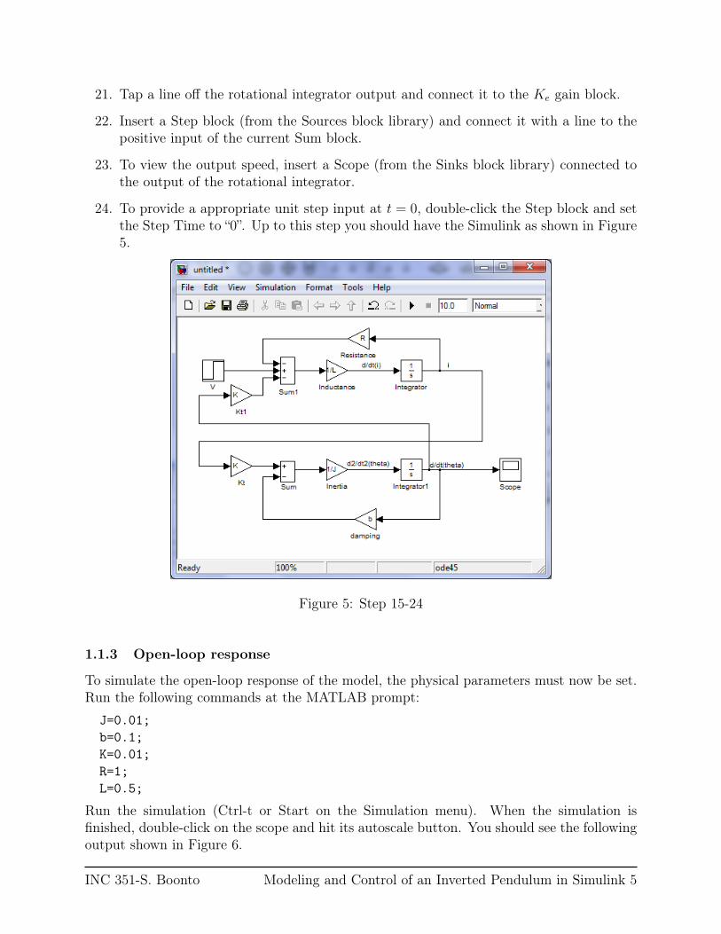
21. Tap a line off the rotational integrator output and connect it to the Ke gain block.

22. Insert a Step block (from the Sources block library) and connect it with a line to thepositive input of the current Sum block.

23. To view the output speed, insert a Scope (from the Sinks block library) connected tothe output of the rotational integrator.

24. To provide a appropriate unit step input at t = 0, double-click the Step block and setthe Step Time to “0”. Up to this step you should have the Simulink as shown in Figure5.

Figure 5: Step 15-24

1.1.3 Open-loop response

To simulate the open-loop response of the model, the physical parameters must now be set.Run the following commands at the MATLAB prompt:

J=0.01;b=0.1;K=0.01;R=1;L=0.5;

Run the simulation (Ctrl-t or Start on the Simulation menu). When the simulation isfinished, double-click on the scope and hit its autoscale button. You should see the followingoutput shown in Figure 6.


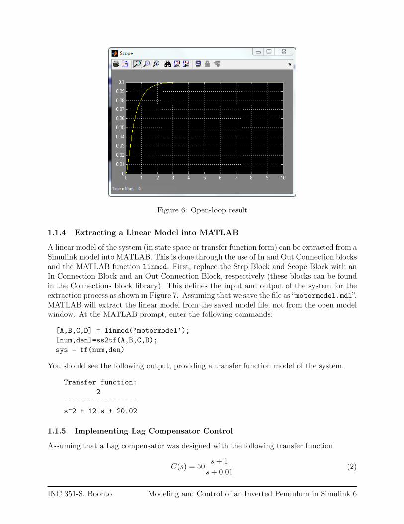
Figure 6: Open-loop result

1.1.4 Extracting a Linear Model into MATLAB

A linear model of the system (in state space or transfer function form) can be extracted from aSimulink model into MATLAB. This is done through the use of In and Out Connection blocksand the MATLAB function linmod. First, replace the Step Block and Scope Block with anIn Connection Block and an Out Connection Block, respectively (these blocks can be foundin the Connections block library). This defines the input and output of the system for theextraction process as shown in Figure 7. Assuming that we save the file as “motormodel.mdl”.MATLAB will extract the linear model from the saved model file, not from the open modelwindow. At the MATLAB prompt, enter the following commands:

[A,B,C,D] = linmod(’motormodel’);[num,den]=ss2tf(A,B,C,D);sys = tf(num,den)

You should see the following output, providing a transfer function model of the system.

Transfer function:2

------------------s^2 + 12 s + 20.02

1.1.5 Implementing Lag Compensator Control

Assuming that a Lag compensator was designed with the following transfer function

C(s) = 50s+ 1

s+ 0.01(2)


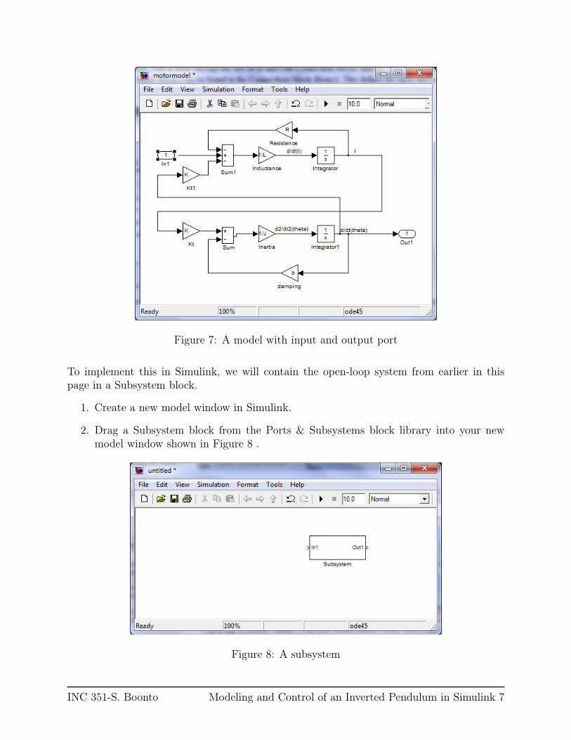
Figure 7: A model with input and output port

To implement this in Simulink, we will contain the open-loop system from earlier in thispage in a Subsystem block.

1. Create a new model window in Simulink.

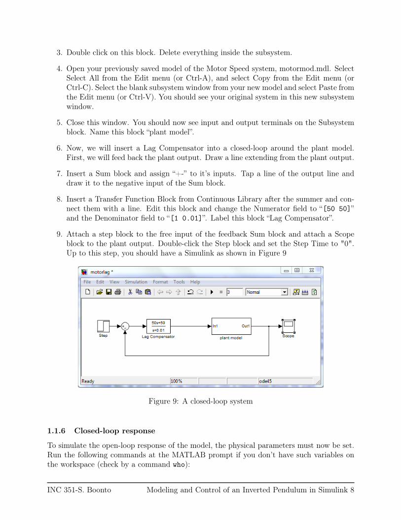
2. Drag a Subsystem block from the Ports & Subsystems block library into your newmodel window shown in Figure 8 .

Figure 8: A subsystem


3. Double click on this block. Delete everything inside the subsystem.

4. Open your previously saved model of the Motor Speed system, motormod.mdl. SelectSelect All from the Edit menu (or Ctrl-A), and select Copy from the Edit menu (orCtrl-C). Select the blank subsystem window from your new model and select Paste fromthe Edit menu (or Ctrl-V). You should see your original system in this new subsystemwindow.

5. Close this window. You should now see input and output terminals on the Subsystemblock. Name this block “plant model”.

6. Now, we will insert a Lag Compensator into a closed-loop around the plant model.First, we will feed back the plant output. Draw a line extending from the plant output.

7. Insert a Sum block and assign “+-” to it’s inputs. Tap a line of the output line anddraw it to the negative input of the Sum block.

8. Insert a Transfer Function Block from Continuous Library after the summer and con-nect them with a line. Edit this block and change the Numerator field to “[50 50]”and the Denominator field to “[1 0.01]”. Label this block “Lag Compensator”.

9. Attach a step block to the free input of the feedback Sum block and attach a Scopeblock to the plant output. Double-click the Step block and set the Step Time to "0".Up to this step, you should have a Simulink as shown in Figure 9

Figure 9: A closed-loop system

1.1.6 Closed-loop response

To simulate the open-loop response of the model, the physical parameters must now be set.Run the following commands at the MATLAB prompt if you don’t have such variables onthe workspace (check by a command who):


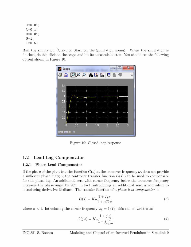
J=0.01;b=0.1;K=0.01;R=1;L=0.5;

Run the simulation (Ctrl-t or Start on the Simulation menu). When the simulation isfinished, double-click on the scope and hit its autoscale button. You should see the followingoutput shown in Figure 10.

Figure 10: Closed-loop response

1.2 Lead-Lag Compensator

1.2.1 Phase-Lead Compensator

If the phase of the plant transfer function G(s) at the crossover frequency ωc does not providea sufficient phase margin, the controller transfer function C(s) can be used to compensatefor this phase lag. An additional zero with corner frequency below the crossover frequencyincreases the phase angel by 90. In fact, introducing an additional zero is equivalent tointroducing derivative feedback. The transfer function of a phase-lead compensator is

C(s) = KP1 + TLs

1 + αTLs(3)

where α < 1. Introducing the corner frequency ωL = 1/TL, this can be written as

C(jω) = KP

1 + j ωωL

1 + j ωωL/α

(4)


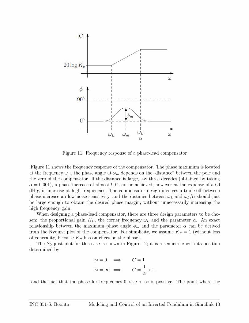
Figure 11: Frequency response of a phase-lead compensator

Figure 11 shows the frequency response of the compensator. The phase maximum is locatedat the frequency ωm, the phase angle at ωm depends on the “distance” between the pole andthe zero of the compensator. If the distance is large, say three decades (obtained by takingα = 0.001), a phase increase of almost 90 can be achieved, however at the expense of a 60dB gain increase at high frequencies. The compensator design involves a trade-off betweenphase increase an low noise sensitivity, and the distance between ωL and ωL/α should justbe large enough to obtain the desired phase margin, without unnecessarily increasing thehigh frequency gain.

When designing a phase-lead compensator, there are three design parameters to be cho-sen: the proportional gain KP , the corner frequency ωL and the parameter α. An exactrelationship between the maximum phase angle ϕm and the parameter α can be derivedfrom the Nyquist plot of the compensator. For simplicity, we assume KP = 1 (without lossof generality, because KP has on effect on the phase).

The Nyquist plot for this case is shown in Figure 12; it is a semicircle with its positiondetermined by

ω = 0 =⇒ C = 1

ω = ∞ =⇒ C =1

α> 1

and the fact that the phase for frequencies 0 < ω < ∞ is positive. The point where the


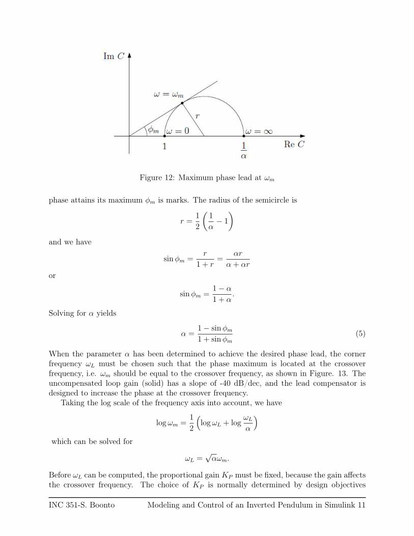
Figure 12: Maximum phase lead at ωm

phase attains its maximum ϕm is marks. The radius of the semicircle is

r =1

2

(1

α− 1

)and we have

sinϕm =r

1 + r=

αr

α + αr

or

sinϕm =1− α

1 + α.

Solving for α yields

α =1− sinϕm

1 + sinϕm

(5)

When the parameter α has been determined to achieve the desired phase lead, the cornerfrequency ωL must be chosen such that the phase maximum is located at the crossoverfrequency, i.e. ωm should be equal to the crossover frequency, as shown in Figure. 13. Theuncompensated loop gain (solid) has a slope of -40 dB/dec, and the lead compensator isdesigned to increase the phase at the crossover frequency.

Taking the log scale of the frequency axis into account, we have

logωm =1

2

(logωL + log

ωL

α

)which can be solved for

ωL =√αωm.

Before ωL can be computed, the proportional gain KP must be fixed, because the gain affectsthe crossover frequency. The choice of KP is normally determined by design objectives


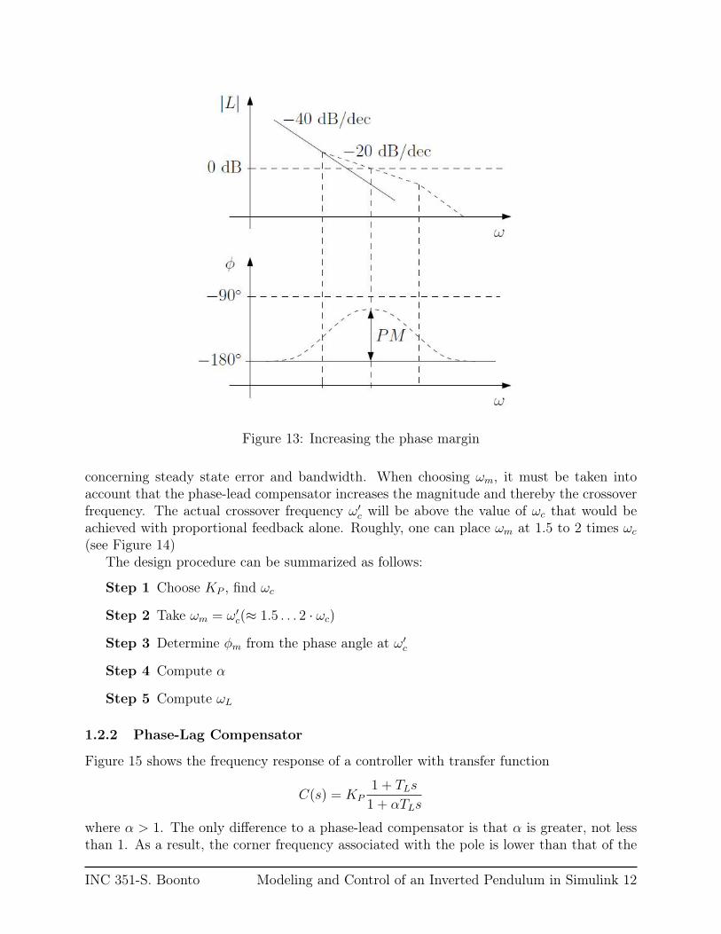
Figure 13: Increasing the phase margin

concerning steady state error and bandwidth. When choosing ωm, it must be taken intoaccount that the phase-lead compensator increases the magnitude and thereby the crossoverfrequency. The actual crossover frequency ω′

c will be above the value of ωc that would beachieved with proportional feedback alone. Roughly, one can place ωm at 1.5 to 2 times ωc

(see Figure 14)The design procedure can be summarized as follows:

Step 1 Choose KP , find ωc

Step 2 Take ωm = ω′c(≈ 1.5 . . . 2 · ωc)

Step 3 Determine ϕm from the phase angle at ω′c

Step 4 Compute α

Step 5 Compute ωL

1.2.2 Phase-Lag Compensator

Figure 15 shows the frequency response of a controller with transfer function

C(s) = KP1 + TLs

1 + αTLs

where α > 1. The only difference to a phase-lead compensator is that α is greater, not lessthan 1. As a result, the corner frequency associated with the pole is lower than that of the


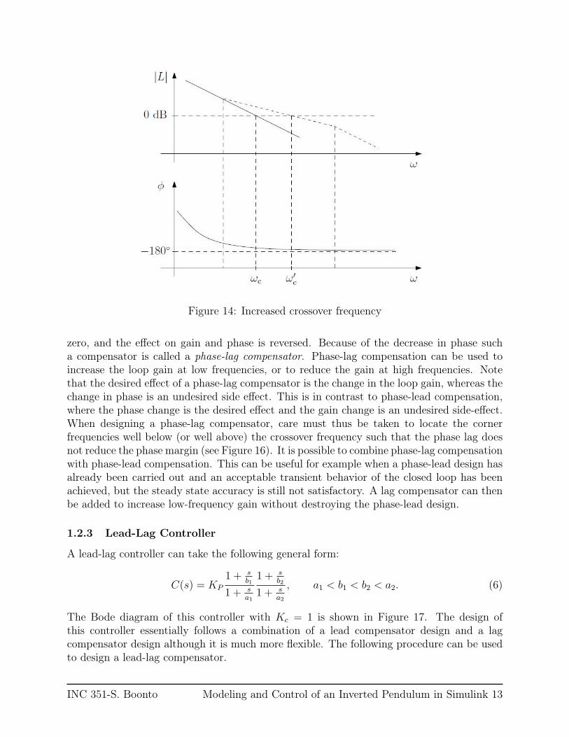
Figure 14: Increased crossover frequency

zero, and the effect on gain and phase is reversed. Because of the decrease in phase sucha compensator is called a phase-lag compensator. Phase-lag compensation can be used toincrease the loop gain at low frequencies, or to reduce the gain at high frequencies. Notethat the desired effect of a phase-lag compensator is the change in the loop gain, whereas thechange in phase is an undesired side effect. This is in contrast to phase-lead compensation,where the phase change is the desired effect and the gain change is an undesired side-effect.When designing a phase-lag compensator, care must thus be taken to locate the cornerfrequencies well below (or well above) the crossover frequency such that the phase lag doesnot reduce the phase margin (see Figure 16). It is possible to combine phase-lag compensationwith phase-lead compensation. This can be useful for example when a phase-lead design hasalready been carried out and an acceptable transient behavior of the closed loop has beenachieved, but the steady state accuracy is still not satisfactory. A lag compensator can thenbe added to increase low-frequency gain without destroying the phase-lead design.

1.2.3 Lead-Lag Controller

A lead-lag controller can take the following general form:

C(s) = KP

1 + sb1

1 + sa1

1 + sb2

1 + sa2

, a1 < b1 < b2 < a2. (6)

The Bode diagram of this controller with Kc = 1 is shown in Figure 17. The design ofthis controller essentially follows a combination of a lead compensator design and a lagcompensator design although it is much more flexible. The following procedure can be usedto design a lead-lag compensator.


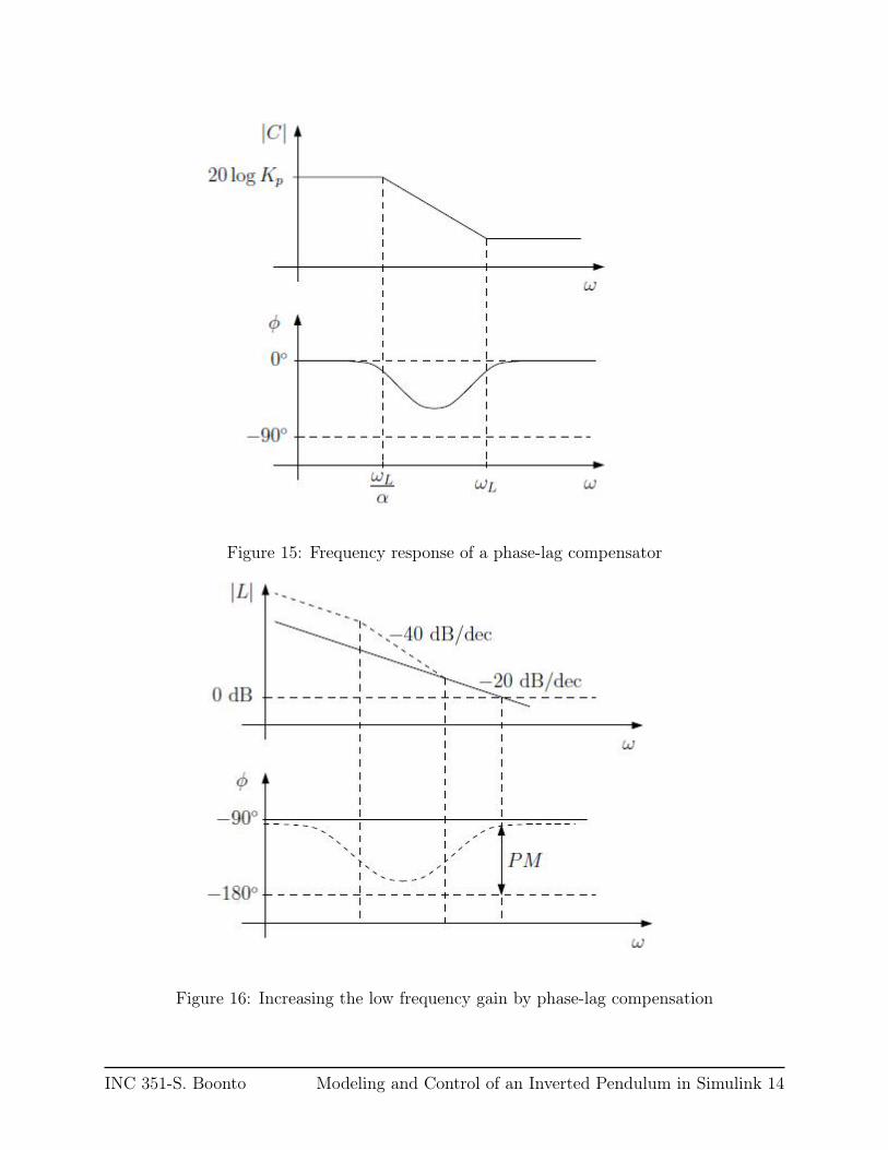
Figure 15: Frequency response of a phase-lag compensator

Figure 16: Increasing the low frequency gain by phase-lag compensation


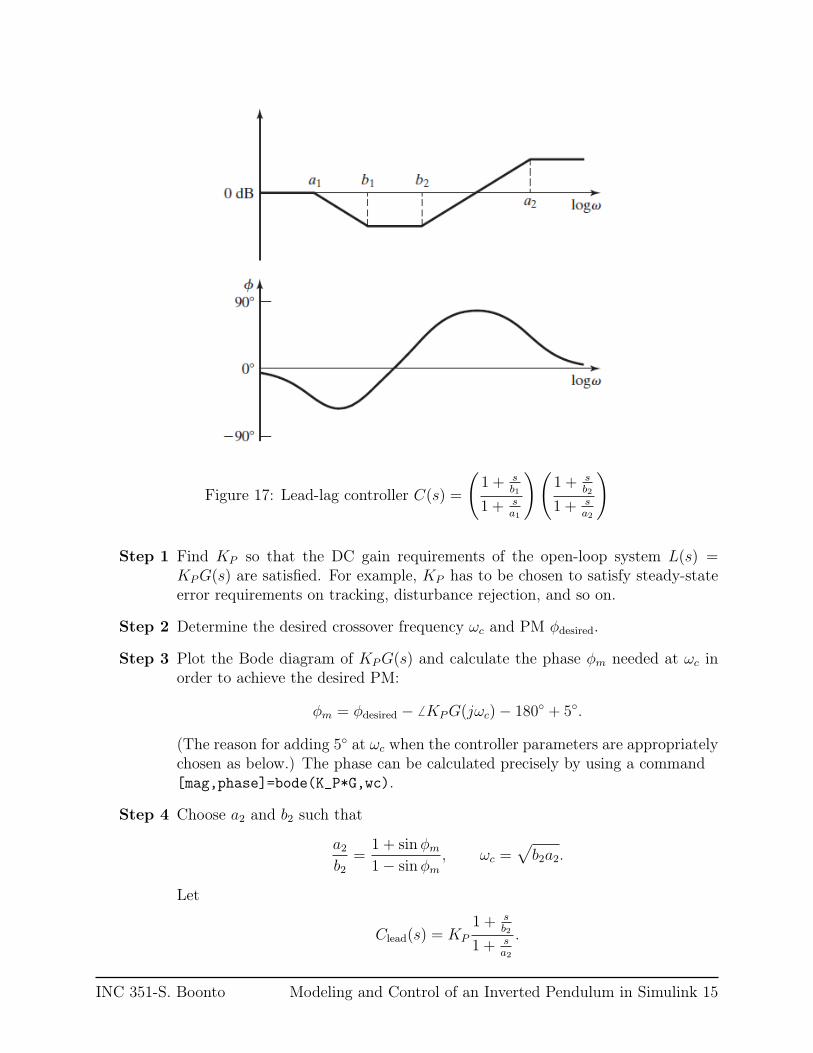
Figure 17: Lead-lag controller C(s) =

(1 + s

b1

1 + sa1

)(1 + s

b2

1 + sa2

)

Step 1 Find KP so that the DC gain requirements of the open-loop system L(s) =KPG(s) are satisfied. For example, KP has to be chosen to satisfy steady-stateerror requirements on tracking, disturbance rejection, and so on.

Step 2 Determine the desired crossover frequency ωc and PM ϕdesired.

Step 3 Plot the Bode diagram of KPG(s) and calculate the phase ϕm needed at ωc inorder to achieve the desired PM:

ϕm = ϕdesired − KPG(jωc)− 180 + 5.

(The reason for adding 5 at ωc when the controller parameters are appropriatelychosen as below.) The phase can be calculated precisely by using a command[mag,phase]=bode(K_P*G,wc).

Step 4 Choose a2 and b2 such that

a2b2

=1 + sinϕm

1− sinϕm

, ωc =√b2a2.

Let

Clead(s) = KP

1 + sb2

1 + sa2

.


Step 5 Choose

b1 ≈ 0.1ωc, a1 =b1

|Clead(jωc)G(jωc)|.

The magnitude can be calculated precisely by using a command[mag,phase]=bode(Clead*G,wc).

Step 6 Plot the Bode diagram of C(s)G(s) and check the design specifications.

2 DC Motor Position Modeling and Control in SimulinkLab Equipment

1. a desktop PC or a Labtop PC with MATLAB

2.1 DC Motor Position Modeling in Simulink

Procedure

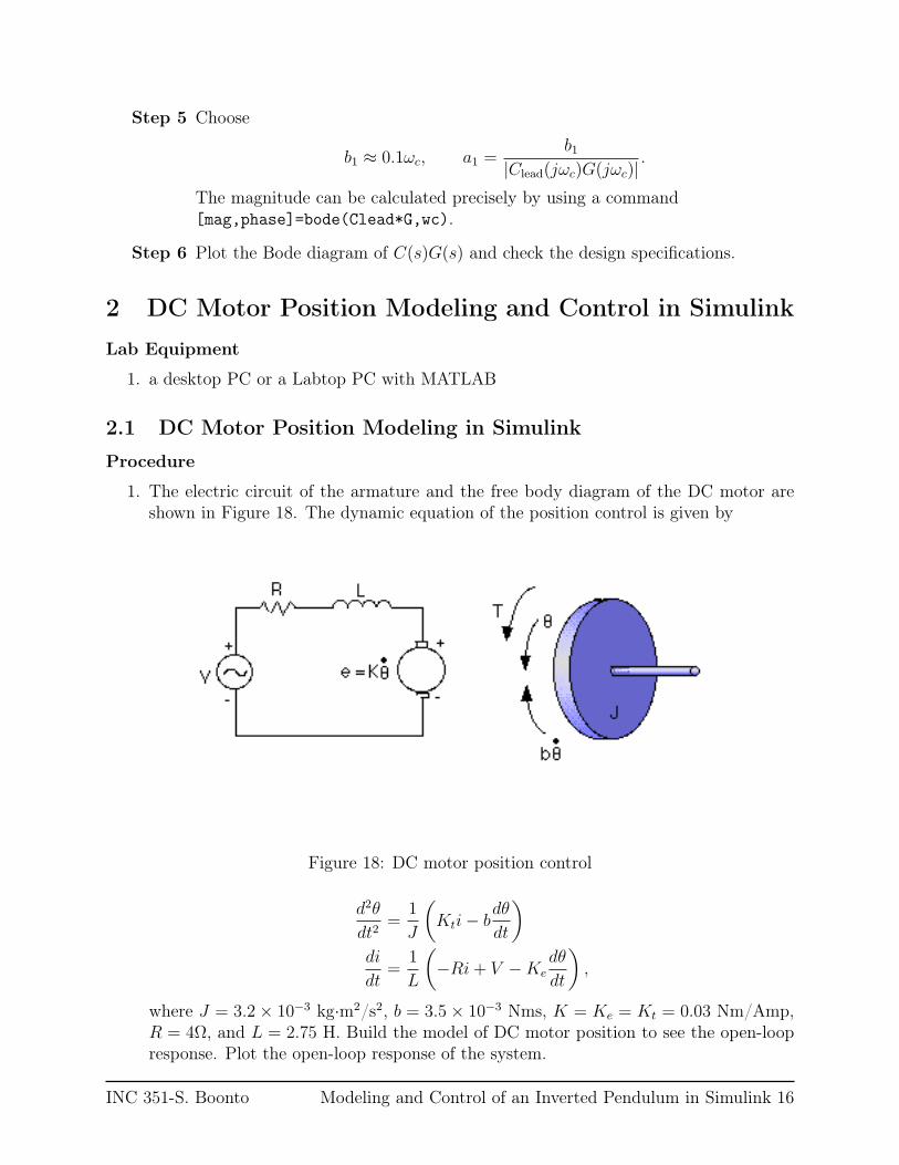
1. The electric circuit of the armature and the free body diagram of the DC motor areshown in Figure 18. The dynamic equation of the position control is given by

Figure 18: DC motor position control

d2θ

dt2=

1

J

(Kti− b

dθ

dt

)di

dt=

1

L

(−Ri+ V −Ke

dθ

dt

),

where J = 3.2× 10−3 kg·m2/s2, b = 3.5× 10−3 Nms, K = Ke = Kt = 0.03 Nm/Amp,R = 4Ω, and L = 2.75 H. Build the model of DC motor position to see the open-loopresponse. Plot the open-loop response of the system.


2. Change the Simulink model into a subsystem form and save it as “motorpos.mdl”.At the MATLAB command prompt, extract the transfer function with the followingcommands:

[A, B, C, D] = linmod(’motorpos’);[num, den] = ss2tf(A,B,C,D);G = tf(num,den)

Check G(s) and assume that the parameters, which are less than 1 × 10−8 are aboutzero. Write down the new approximate transfer function as G1(s).

3. Plot Bode diagram of G1(s). What is PM of G1(s).

4. Design a lead-lag compensator C(s) for G1(s). The control objectives are

• a rise time of tr = 1.7s (Hint: tr ≈ 1.7ωc

)

• a phase margin of PM = 50.

• the steady-state error with respect to a ramp input is no greater than 0.02. (Hint:Use

e(∞) = lims→0

s1

1 + L(s)

1

s2

to find the steady-state error.)

5. Connect the controller C(s) into your Simulink model and plot the closed-loop responsewith respect to a ramp input.

3 Report1. Your report should include:

• all necessary Bode diagrams .• discuss your final results and explain how to improve the results.

The discussion should be made in both theoretical and experimental perspectives. Thestudent who shows some useful extra jobs will get bonus points.

2. Data can be copied, but do not photocopy the graph. Each student should plot his orher own.

3. Duplicate reports are totally unacceptable and no marks will be grade to all responsiblestudents.

4. The report is due before you arrive for the next lab, which is usually a week after thelab. Late reports will not be accepted.


Documents

Laboratory DC Motor Position Modeling and Control in Simulinkinc.kmutt.ac.th/course/inc354/lead_lagv3.pdf · Laboratory DC Motor Position Modeling and Control in Simulink Objectives: