Laboratory Experiment 8: 

DC Motor Control  

        

  

Presented to the University of California, San Diego 

Department of Mechanical and Aerospace Engineering MAE 170 

           

Prepared by Kimberly Nguyen, A05 Grace Victorine, A05 

5/28/15    

 

Abstract ______________________________________________  The purpose of this experiment was to explore the behavior, system gains, and feedback of a position control                                   system. The control effort was determined to be proportional to gain, such that an increase in gain led to an                                       increase in error. Calibration of the feedback potentiometer provided a linear fit indicating sensitivity of                             0.086 V/degree. Calibrating the knob gain and calculated gain from measured resistance led to a 1:0.423 ratio,                                 which is a 57.7% error from the theoretical 1:1 ratio. Investigation of the relationship between error and gain                                   led to a results indicating that as gain increased, error voltage decreased. Then, an experimental trial was                                 conducted to determine how useful the calibration of the feedback potentiometer was: the percent error in                               discrepancy between the predicted and experimental angles were 6.41% for +5V and 4.03% for -5V. Graphs                               in the final part of this experiment provided results indicating that when gain increased, oscillations                             increased at the feedback signal, op-amp, and motor drive, while steady state errors, rise times, and                               overshoot stayed relatively constant. As well, it was shown that as gain increased, the settling times for the                                   op-amp and feedback signal were likewise increased. The settling time approached zero for the motor drive.                           

1 

I.  Introduction ______________________________________________  The DC Motor, or servo motor has been used widely to power all sorts of machines, from inkjet printers, to                                       model airplanes, to communications satellites. DC motors function by converting voltage potential                       differences into mechanical energy. The internal mechanism causes periodic change in the current flow.                           Inside the motor and North and South designated magnets of opposite polarities. This internal rotation                             creates a torque  that powers the motor.   The servomechanism is composed of an actuator (usually a DC motor), a controller, and a sensor. The                                 controller amplifies instrumentation, the driver is composed of two transistors, and the sensor is combined                             with the mechanical feedback structure in the potentiometer. The controller accepts two input voltages; the                             position command, or what is desired and the feedback voltage which is the actual voltage. Ideally, the two                                   voltages should be equal so the instrument amplifier determines the difference between the two, called the                               error, and multiplies it by the gain to produce and output voltage known as the control effort. The control                                     effort is applied to the resistors and results in motion of the motor. As the motion continues, the resulting                                     feedback voltage is continuously fed to the control amplifier. This process is iterated in a closed loop to allow                                     the system to arrive at and maintain the desired position.  II.  Theory ______________________________________________ 

 Figure 1: Representation of Feedback Control System 1  Figure 2: Typical System Response to Step Change 1 

Figure 1 depicted the feedback control system of the servomechanism. In order to calculate the voltage difference between the command and feedback voltages, the following equation was used: 

ontrol Effort ain rror  C = G * E                                                   ( 1) 1  The amplifier gain was determined by the following equation in which R G  represented the gain resistor: 

Gain =( 1+50/R G ) (2) 1 

The Proportional-Integral-Derivative (PID) controller was characterised by the following equation with with K p  as the Proportional gain, used to affect rise time, K p  as the Integral gain, used to affect steady state error, K p  as the Derivative gain, used to control overshoot, e as the Error = Set Point – Process Variable, and t 

as with respect to time:                               (t) e(t)  (t)dt e(t)u = Kp + K1∫t

0e + Kd ddt                                  (3) 2 

The PID function is illustrated in Figure 2. The rise time indicates the necessary elapsed time for the signal to                                       reach the set point. The percent overshoot indicates the extent to which the signal originally surpasses the set                                   point. The settling time is time it take for the signal to settle within some error of the set point. The                                         steady-state error is the offset between the settled signal and the set point.  

2 

III.  Experimental Procedures ______________________________________________  

Part I: Sensor Verification and Calibration 

          Figure 3: Simplified  Schematic of Control Board 1  Figure 4: Pictorial Control Board Schematic 1 

 Figure 3 depicted the simplified electronic schematic of the control board which detailed the individual                             components such as resistors, voltage supplies, transistors, gain resistors, and motor drives. Figure 4                           delineated the layout of the physical board that was to be worked on and illustrated where to connect the                                     desired wires in the first part of the experiment. In the first part of the experiment, the CMD mode switch                                       was turned to “Manual” and “Power In” was attached to the control board with +15V, -15V and Gnd from the                                       protoboard. The three potentiometer wires were attached to the 3-Position Feedback terminal. The DMM                           was used to measure the feedback voltage from the sensor. The driven wheel was turned fully counter                                 clockwise and the resulting voltage as well as degrees indicated by the arrow were noted at test point 3. The                                       measurement was repeated at 50-degree increments in the clockwise direction and data were recorded.  

Part II: Calibration of the gain adjustment knob 

 Figure 5: Diagram of the Instrumentation Amplifier 

 Figure 5 delineated the setup of the instrument amplifier which was used in Part II of the experiment in order                                       to determine the relationship between the gain control knob’s position and true gain. Power was turned off,                                 then the multimeter was attached to the two white gain wires. The initial position to which the gain knob                                     was set was “10”. Infinite resistance was registered at this point. subsequently decreasing resistances were                             registered at gain resistances that increased in increments of 10. Upon the recording of all resistances, the                                 gain and resistance were plotted to a linear fit with the x-axis displaying the knob setting and the y-axis                                     displaying the calculated gain.  

3 

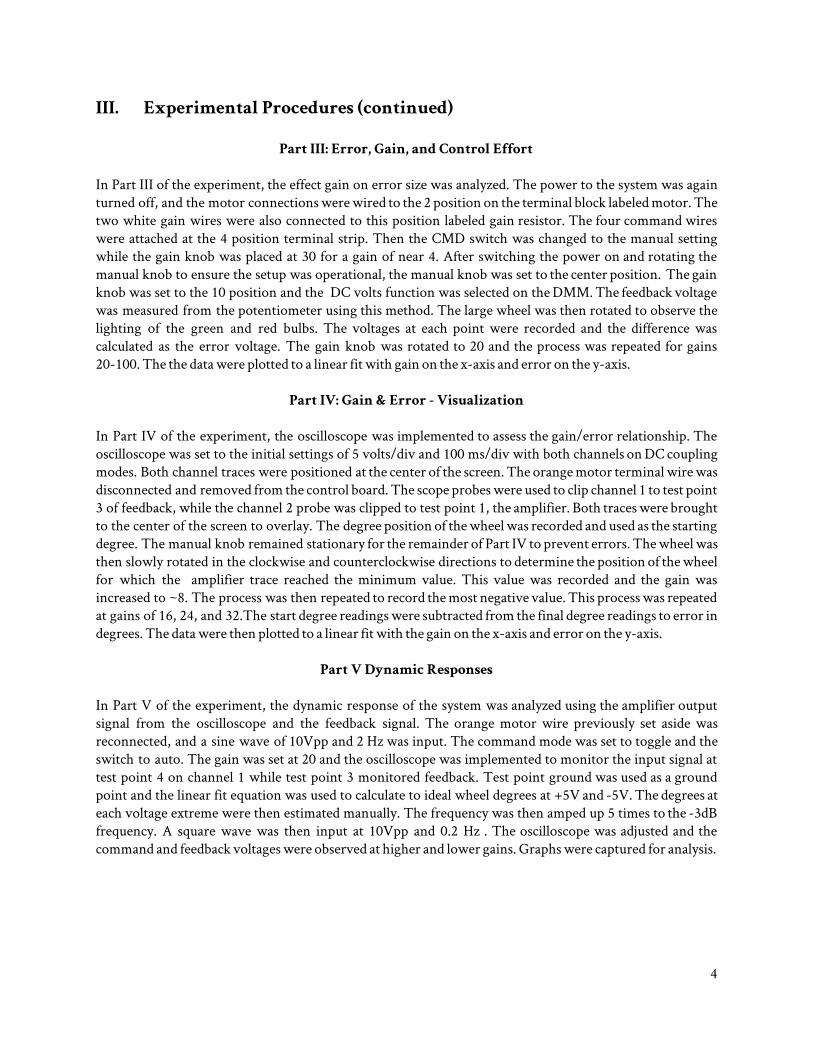
III.  Experimental Procedures (continued)  

Part III: Error, Gain, and Control Effort  

In Part III of the experiment, the effect gain on error size was analyzed. The power to the system was again                                         turned off, and the motor connections were wired to the 2 position on the terminal block labeled motor. The                                     two white gain wires were also connected to this position labeled gain resistor. The four command wires                                 were attached at the 4 position terminal strip. Then the CMD switch was changed to the manual setting                                   while the gain knob was placed at 30 for a gain of near 4. After switching the power on and rotating the                                           manual knob to ensure the setup was operational, the manual knob was set to the center position. The gain                                     knob was set to the 10 position and the DC volts function was selected on the DMM. The feedback voltage                                       was measured from the potentiometer using this method. The large wheel was then rotated to observe the                                 lighting of the green and red bulbs. The voltages at each point were recorded and the difference was                                   calculated as the error voltage. The gain knob was rotated to 20 and the process was repeated for gains                                     20-100. The the data were plotted to a linear fit with gain on the x-axis and error on the y-axis.  

Part IV: Gain & Error - Visualization  

In Part IV of the experiment, the oscilloscope was implemented to assess the gain/error relationship. The                               oscilloscope was set to the initial settings of 5 volts/div and 100 ms/div with both channels on DC coupling                                     modes. Both channel traces were positioned at the center of the screen. The orange motor terminal wire was                                   disconnected and removed from the control board. The scope probes were used to clip channel 1 to test point                                     3 of feedback, while the channel 2 probe was clipped to test point 1, the amplifier. Both traces were brought                                       to the center of the screen to overlay. The degree position of the wheel was recorded and used as the starting                                         degree. The manual knob remained stationary for the remainder of Part IV to prevent errors. The wheel was                                   then slowly rotated in the clockwise and counterclockwise directions to determine the position of the wheel                               for which the amplifier trace reached the minimum value. This value was recorded and the gain was                                 increased to ~8. The process was then repeated to record the most negative value. This process was repeated                                   at gains of 16, 24, and 32.The start degree readings were subtracted from the final degree readings to error in                                       degrees. The data were then plotted to a linear fit with the gain on the x-axis and error on the y-axis.  

Part V Dynamic Responses  

In Part V of the experiment, the dynamic response of the system was analyzed using the amplifier output                                   signal from the oscilloscope and the feedback signal. The orange motor wire previously set aside was                               reconnected, and a sine wave of 10Vpp and 2 Hz was input. The command mode was set to toggle and the                                         switch to auto. The gain was set at 20 and the oscilloscope was implemented to monitor the input signal at                                       test point 4 on channel 1 while test point 3 monitored feedback. Test point ground was used as a ground                                       point and the linear fit equation was used to calculate to ideal wheel degrees at +5V and -5V. The degrees at                                         each voltage extreme were then estimated manually. The frequency was then amped up 5 times to the -3dB                                   frequency. A square wave was then input at 10Vpp and 0.2 Hz . The oscilloscope was adjusted and the                                     command and feedback voltages were observed at higher and lower gains. Graphs were captured for analysis.     

4 

IV.  Data and Results ______________________________________________  

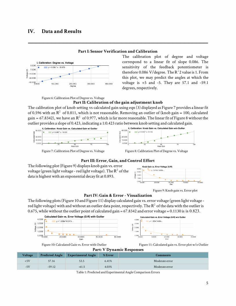
Part I: Sensor Verification and Calibration The calibration plot of degree and voltage             correspond to a linear fit of slope 0.086. The                 sensitivity of the feedback potentiometer is           therefore 0.086 V/degree. The R^2 value is 1. From                 this plot, we may predict the angles at which the                   voltage is +5 and -5. They are 57.1 and -59.1                   degrees, respectively. 

 Figure 6: Calibration Plot of Degree vs. Voltage 

Part II: Calibration of the gain adjustment knob The calibration plot of knob setting vs calculated gain using eqn (3) displayed as Figure 7 provides a linear fit                                       of 0.596 with an R 2 of 0.811, which is not reasonable. Removing an outlier of (knob gain = 100, calculated                                         gain = 67.8342), we have an R 2 of 0.977, which is far more reasonable. The linear fit of Figure 8 without the                                             outlier provides a slope of 0.423, indicating a 1:0.423 ratio between knob setting and calculated gain.  

 Figure 7: Calibration Plot of Degree vs. Voltage Figure 8: Calibration Plot of Degree vs. Voltage 

 Part III: Error, Gain, and Control Effort 

The following plot (Figure 9) displays knob gain vs. error voltage (green light voltage - red light voltage). The  R 2   of the data is highest with an exponential decay fit at 0.893.    

Figure 9: Knob gain vs. Error plot   Part IV: Gain & Error - Visualization   

The following plots (Figure 10 and Figure 11) display calculated gain vs. error voltage (green light voltage - red light voltage) with and without an outlier data point, respectively. The  R 2   of the data with the outlier is 0.675, while without the outlier point of calculated gain = 67.8342 and error voltage = 0.1130 is  is 0.823.  

 Figure 10: Calculated Gain vs. Error with Outlier Figure 11: Calculated gain vs. Error plot w/o Outlier 

Part: V Dynamic Responses Voltage  Predicted Angle  Experimental Angle  % Error  Comments 

+5V  57.16  53.5  6.41%  Moderate error 

-5V  -59.12  -61.5  4.03%  Moderate error 

Table 1: Predicted and Experimental Angle Comparison Errors 

5 

IV.  Data and Results (continued) TP 4 and 3 

 Figure 12: Gain = 2.00 Figure 13: Gain = 24.27 Figure 14: Gain = 32.00 

The graphs above depict the corresponding gain setting and frequencies that label them. The input of                               channel 1 (blue) is at the command point, test-point 4 (TP4), and channel 2 (pink) is at the feedback signal                                       (TP3). The behavior indicates that oscillation increases as gain increases. As well, overshoot, rise time, and                               steady state errors are constant throughout the gain changes.   

TP 4 and 1 

 Figure 15: Gain = 2.00  Figure 16: Gain = 24.27 Figure 17: Gain = 32.00 

The graphs above depict the corresponding gain setting and frequencies that label them. The input of                               channel 1 (blue) is at the command point, test-point 4 (TP4), and channel 2 (pink) is at the op-amp output                                       (TP1). The behavior indicates that oscillation increases largely as gain increases. As well, overshoot, rise                             time, and steady state errors are constant throughout the gain changes.  Settling approaches nonexistence.  

TP 4 and 2 

 Figure 18: Gain = 2.00 Figure 19: Gain =24.27 Figure 20: Gain = 32.00 The graphs above depict the corresponding gain setting and frequencies that label them. The input of                               channel 1 (blue) is at the command point, test-point 4 (TP4), and channel 2 (pink) is at the motor drive (TP2).                                         The behavior indicates that oscillation increases largely as gain increases. As well, overshoot, rise time, and                               steady state errors are constant throughout the gain changes.  Settling approaches zero.  

6 

V.  Discussion and Error Analysis ______________________________________________  In the first part of this experiment, a potentiometer was calibrated using angle and voltage data alongside a                                   linear fit. The sensitivity was found to be 0.0817 V/degree. Using this sensitivity, angle predictions were                               made for +5V and -5V, which were 57.16 and -59.12 degrees, respectively. This resulted in a 6.41% error for                                     +5V experimental angle of 53.5 degrees and a 4.03% error for the -5V experimental angle of -61.5 degrees                                   (Table 1). Because no systematic method was used to determine experimental angles, it is likely that the                                 minor discrepancies between the calculated angle and the experimental angle were due to human sight error.  For the second part of this experiment, the gain knob was calibrated to the gain calculated from the measured                                     resistance. With a notable outlier, the original fit of the gain knob resulted in a slope of 0.596, an R 2  of 0.811                                           (Figure 7). Without the outlier, the fit provided a slope of 0.423, resulting in a larger R 2 of 0.977, indicating                                        higher level of linearity (Figure 8). The fit with the higher R 2  provides a sensitivity of 1:0.4298 V/degree.                                   This is with consideration of a linear fit; however, upon closer inspection of the data (Table 3) and the                                     schematic of the op-amps (Figure 5), the shifting pattern of the slopes at intervals appear to correspond to the                                     addition of the gain of another amplifier. In which case, the outlier is not actually an outlier at all.   In the third part of this experiment, it was noticeable that as gain increased, the error voltage exponentially                                   decayed (Figure 9). Even more notable was the amplifier attempting to control the motor when the                               calculated control effort was high enough. The wheel was far more difficult to turn at higher gains. This was                                     most likely due to the smaller errors required of systems to produce the necessary output voltage to turn the                                     wheel. The force applied by the motor was theoretically higher when the potentiometer sensitivity was                             increased. The amplifier began trying to control the motor when the wheel was turned at a higher gain. The                                     wheel was more difficult to turn as the gain increased.  In the fourth part of this experiment, an oscilloscope was used to graphically explore the relationship                               between gain and error. Exponential decay behavior was observed in the graphs of part four (Figure 12-20),                                 indicating a decrease in error as calculated gain increased. This was theoretically due to the potentiometer,                               which reacts more sensitively to higher gains than lower ones, thus resulting in smaller errors.   In the final part of this experiment, the linear fit from data in the first part of this experiment was used to                                           predict the angle of displacement in the potentiometer, whose error was discussed previously. In addition,                             the -3dB frequency was calculated to be 5.69 Hz. At a frequency was 28.45 Hz, which is 5 times that of the                                           -3dB, the motor stopped responding to the command signal. This was likely due to the frequency being too                                   high, a situation which reasonably may lead to loss of control over the movement of the wheel. The limiting                                     factor would then be the frequency response. From the screenshots captured, it was concluded that as gain                                 increased, rise times, overshoot, and steady state errors stayed relatively constant while oscillations for the                             motor drive, op-amp, and feedback signal increased. As well, it was shown that as gain increased, the settling                                   times for the op-amp and feedback signal were increased. The settling time approached zero for motor drive.      

7 

VI.  Conclusions ______________________________________________  Ultimately, this experiment demonstrates that the PID controller utilizing a DC motor operates successfully                           to determine and correct for error in position placement. The drawback is that its specificity is heavily reliant                                   on the precision of the DC motor. As demonstrated in Part III of the experiment, increases in gain result in                                       decreases in error. However, as seen in Part V, this decrease in error corresponds with oscillations for the                                   motor, op-amp, and feedback signal all increased. This could mar the quality of the signal, potentially                               negating the benefit of reduced error. This precision is key in designing an ideal PID controller that is able to                                       posit to the specificity desired.    

8 

VII.  References ______________________________________________  

1. Nicholas Busan, Steve Roberts, and Rahul Kapadia. “Experiment 8A/B: DC Motor Control.” (2013). UCSD MAE 170. Web. 19 May. 2015.  < http://mae170.eng.ucsd.edu/lab-procedures > 

2. Joon Lee. “MAE 170 Lecture 8: Introduction to Position Control.” (2015). UCSD MAE 170. Web. 18 May. 2015.  < http://mae170.eng.ucsd.edu/course-lectures >  

     

9 

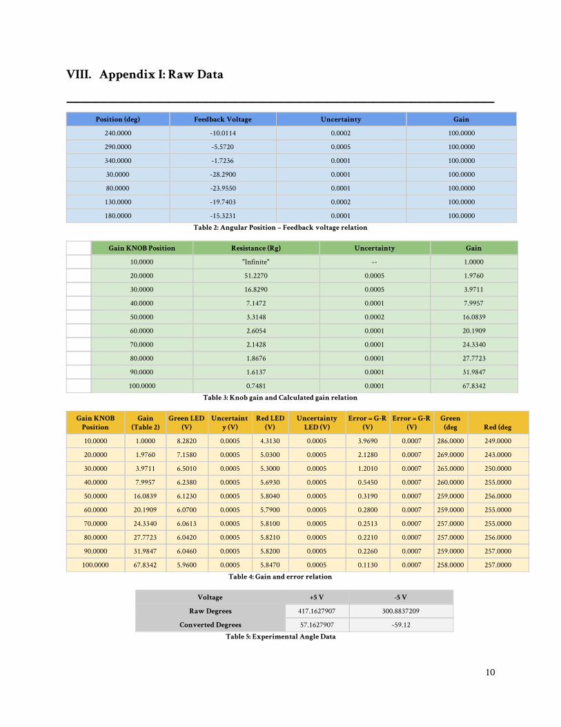
VIII.  Appendix I: Raw Data ______________________________________________  

Position (deg)  Feedback Voltage  Uncertainty  Gain 

240.0000  -10.0114  0.0002  100.0000 

290.0000  -5.5720  0.0005  100.0000 

340.0000  -1.7236  0.0001  100.0000 

30.0000  -28.2900  0.0001  100.0000 

80.0000  -23.9550  0.0001  100.0000 

130.0000  -19.7403  0.0002  100.0000 

180.0000  -15.3231  0.0001  100.0000 Table 2: Angular Position – Feedback voltage relation 

   Gain KNOB Position  Resistance (Rg)  Uncertainty  Gain 

  10.0000  "Infinite"  --  1.0000 

  20.0000  51.2270  0.0005  1.9760 

  30.0000  16.8290  0.0005  3.9711 

  40.0000  7.1472  0.0001  7.9957 

  50.0000  3.3148  0.0002  16.0839 

  60.0000  2.6054  0.0001  20.1909 

  70.0000  2.1428  0.0001  24.3340 

  80.0000  1.8676  0.0001  27.7723 

  90.0000  1.6137  0.0001  31.9847 

  100.0000  0.7481  0.0001  67.8342 Table 3: Knob gain and Calculated gain relation 

 Gain KNOB Position 

Gain (Table 2) 

Green LED (V) 

Uncertainty (V) 

Red LED (V) 

Uncertainty LED (V) 

Error = G-R (V) 

Error = G-R (V) 

Green (deg  Red (deg 

10.0000  1.0000  8.2820  0.0005  4.3130  0.0005  3.9690  0.0007  286.0000  249.0000 

20.0000  1.9760  7.1580  0.0005  5.0300  0.0005  2.1280  0.0007  269.0000  243.0000 

30.0000  3.9711  6.5010  0.0005  5.3000  0.0005  1.2010  0.0007  265.0000  250.0000 

40.0000  7.9957  6.2380  0.0005  5.6930  0.0005  0.5450  0.0007  260.0000  255.0000 

50.0000  16.0839  6.1230  0.0005  5.8040  0.0005  0.3190  0.0007  259.0000  256.0000 

60.0000  20.1909  6.0700  0.0005  5.7900  0.0005  0.2800  0.0007  259.0000  255.0000 

70.0000  24.3340  6.0613  0.0005  5.8100  0.0005  0.2513  0.0007  257.0000  255.0000 

80.0000  27.7723  6.0420  0.0005  5.8210  0.0005  0.2210  0.0007  257.0000  256.0000 

90.0000  31.9847  6.0460  0.0005  5.8200  0.0005  0.2260  0.0007  259.0000  257.0000 

100.0000  67.8342  5.9600  0.0005  5.8470  0.0005  0.1130  0.0007  258.0000  257.0000 Table 4: Gain and error relation 

 Voltage  +5 V  -5 V 

Raw Degrees  417.1627907  300.8837209 

Converted Degrees  57.1627907  -59.12 Table 5: Experimental Angle Data 

10