Laboratory Manual NE03 - Faraday's Law of Induction ...physlab/fundamental/NE03_LM.pdf · NE03 - Faraday's Law of Induction Page 3 of 12 by their distances from a reference point

Version 2.2

NE03 - Faraday's Law of Induction

Page 1 of 12

Laboratory Manual

NE03 - Faraday's Law of Induction Department of Physics

The University of Hong Kong

Aims

To demonstrate various properties of Faraday’s Law such as:

1. Verify the law.

2. Demonstrate the lightly damped oscillation of the hall probe as a simple pendulum.

3. Find the amount of energy lost due to lightly damped oscillation.

Self-learning material: Theory - Background Information

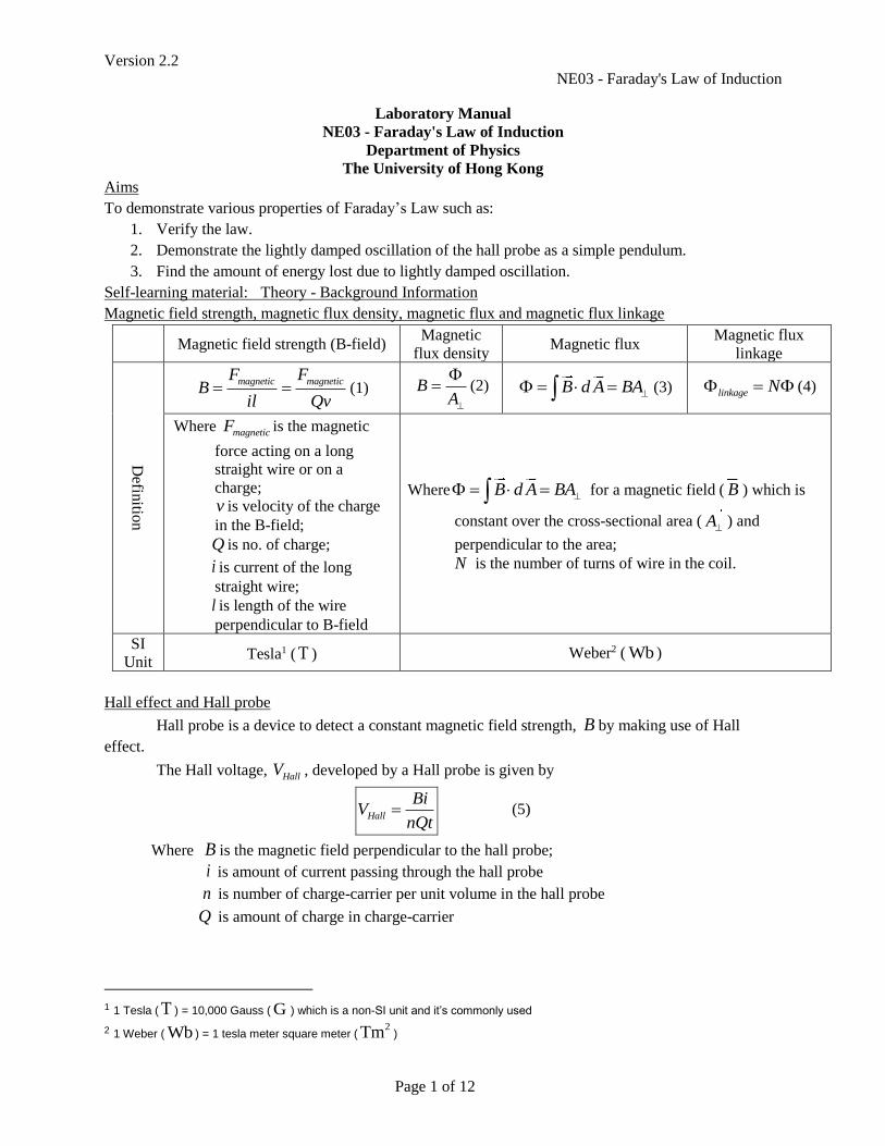
Magnetic field strength, magnetic flux density, magnetic flux and magnetic flux linkage

Magnetic field strength (B-field) Magnetic

flux density Magnetic flux

Magnetic flux

linkage

Defin

ition

magnetic magneticF FB

il Qv (1) B

A

(2) B d A BA (3) linkage N (4)

Where magneticF is the magnetic

force acting on a long

straight wire or on a

charge;

v is velocity of the charge

in the B-field;

Q is no. of charge;

i is current of the long

straight wire;

l is length of the wire

perpendicular to B-field

Where B d A BA for a magnetic field ( B ) which is

constant over the cross-sectional area ( A) and

perpendicular to the area;

N is the number of turns of wire in the coil.

SI

Unit Tesla1 ( T ) Weber2 ( Wb )

Hall effect and Hall probe

Hall probe is a device to detect a constant magnetic field strength, B by making use of Hall

effect.

The Hall voltage, HallV , developed by a Hall probe is given by

Hall

BiV

nQt (5)

Where B is the magnetic field perpendicular to the hall probe;

i is amount of current passing through the hall probe

n is number of charge-carrier per unit volume in the hall probe

Q is amount of charge in charge-carrier

1 1 Tesla ( T ) = 10,000 Gauss ( G ) which is a non-SI unit and it’s commonly used

2 1 Weber ( Wb ) = 1 tesla meter square meter (2Tm )

Version 2.2


Page 2 of 12

Faraday's Law of Induction

(a) Statement

Faraday’s law states that

(b) Mathematical treatment

According to Faraday's Law of Induction, a changing magnetic flux through a coil induces an

electromotive force (e.m.f.) given by induced

dN

dt

(6)

where B d A BA for a magnetic field ( B ) which is constant over the cross-sectional

area ( A) and perpendicular to the area. N is the number of turns of wire in the coil.

For finding average e.m.f., the equation (6) could approximately equal to

induced

dN N

dt t

induced

BAN

t

BA and A is a constant and

independent of time ( t ). induced

BNA

t

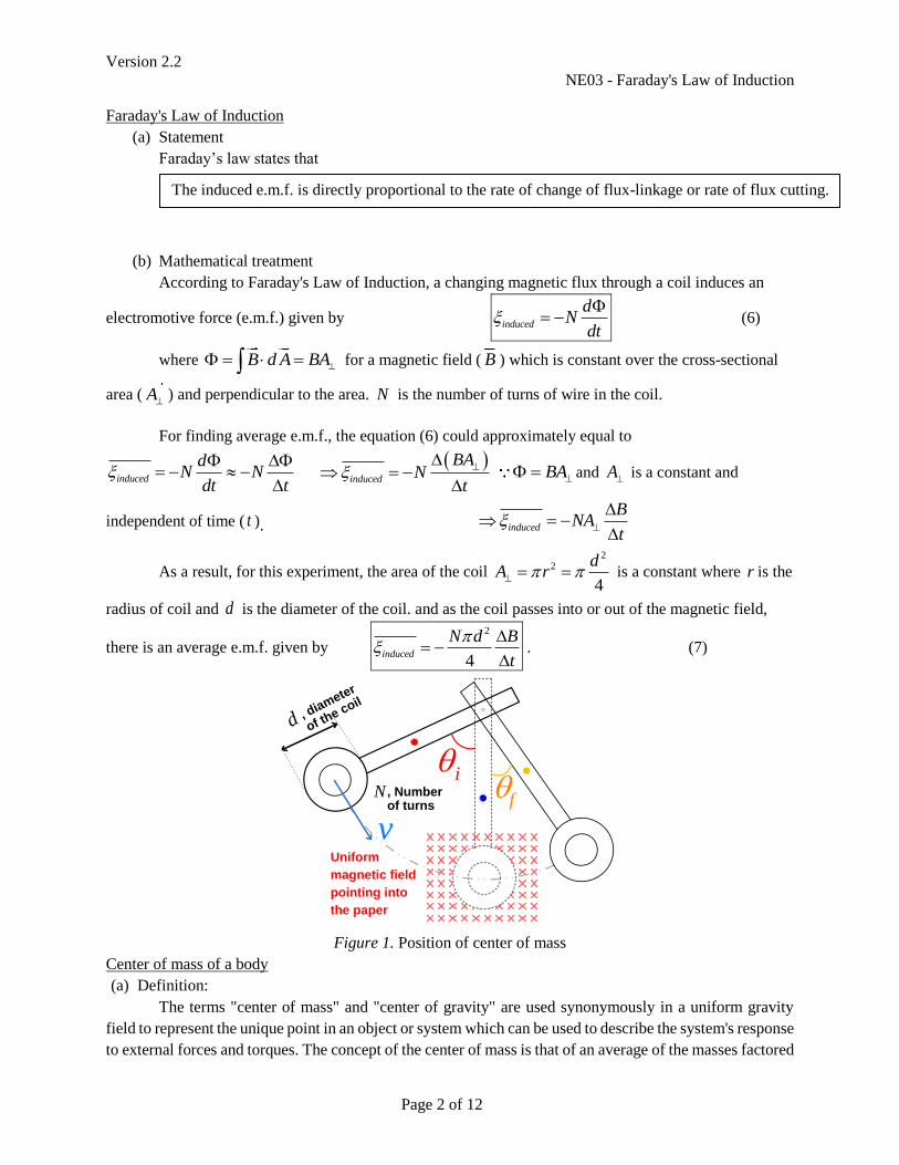
As a result, for this experiment, the area of the coil

22

4

dA r

is a constant where r is the

radius of coil and d is the diameter of the coil. and as the coil passes into or out of the magnetic field,

there is an average e.m.f. given by

2

4induced

N d B

t

. (7)

Uniform

magnetic field

pointing into

the paper

if

v

N , Number of turns

d , diameter

of the coil

Figure 1. Position of center of mass

Center of mass of a body

(a) Definition:

The terms "center of mass" and "center of gravity" are used synonymously in a uniform gravity

field to represent the unique point in an object or system which can be used to describe the system's response

to external forces and torques. The concept of the center of mass is that of an average of the masses factored

The induced e.m.f. is directly proportional to the rate of change of flux-linkage or rate of flux cutting.

Version 2.2


Page 3 of 12

by their distances from a reference point. In one plane, that is like the balancing of a seesaw about a pivot

point with respect to the torques produced.

1x

2xcmx

1m2m

Centre of mass

1 21 2

1 2 1 2

cm

m mx x x

m m m m

Figure 2. Definition center of mass

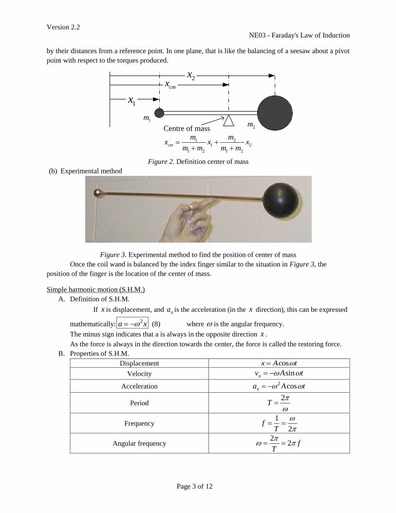
(b) Experimental method

Figure 3. Experimental method to find the position of center of mass

Once the coil wand is balanced by the index finger similar to the situation in Figure 3, the

position of the finger is the location of the center of mass.

Simple harmonic motion (S.H.M.)

A. Definition of S.H.M.

If x is displacement, and xa is the acceleration (in the x direction), this can be expressed

mathematically: 2a x (8) where is the angular frequency.

The minus sign indicates that a is always in the opposite direction x .

As the force is always in the direction towards the center, the force is called the restoring force.

B. Properties of S.H.M.

Displacement cosx A t

Velocity sinxv A t

Acceleration 2 cosxa A t

Period 2

T

Frequency 1

2f

T

Angular frequency 2

2 fT

Version 2.2


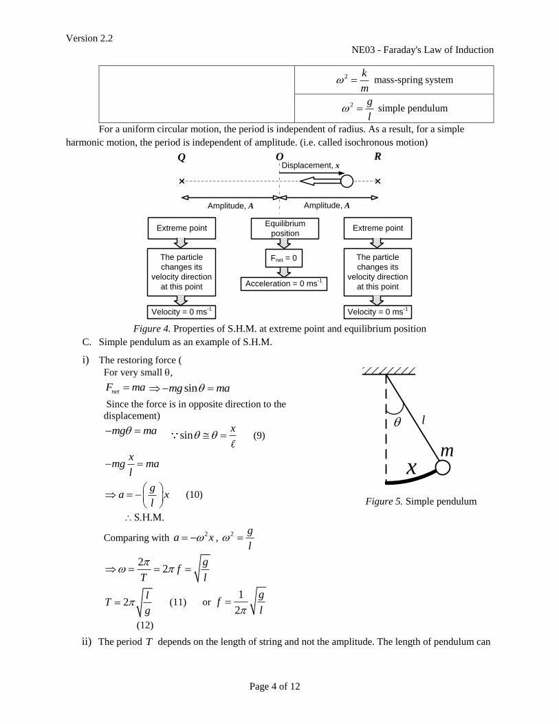
Page 4 of 12

2 k

m mass-spring system

2 g

l simple pendulum

For a uniform circular motion, the period is independent of radius. As a result, for a simple

harmonic motion, the period is independent of amplitude. (i.e. called isochronous motion)

O

Amplitude, AAmplitude, A

Displacement, xQ R

Extreme point

The particle

changes its

velocity direction

at this point

Velocity = 0 ms-1

Extreme point

The particle

changes its

velocity direction

at this point

Velocity = 0 ms-1

Equilibrium

position

Fnet = 0

Acceleration = 0 ms-1

Figure 4. Properties of S.H.M. at extreme point and equilibrium position

C. Simple pendulum as an example of S.H.M.

i) The restoring force (

For very small ,

netF ma sinmg ma

Since the force is in opposite direction to the

displacement)

mg ma sinx

(9)

xmg ma

l

ga x

l

(10)

S.H.M.

Comparing with 2a x ,

2 g

l

22

gf

T l

2l

Tg

(11) or 1

2

gf

l

(12)

x

l

m

Figure 5. Simple pendulum

ii) The period T depends on the length of string and not the amplitude. The length of pendulum can

Version 2.2


Page 5 of 12

be adjusted so that the period is 1 second. (Clock)This is one of the way to find the gravitational

acceleration g by the measuring the period and the length of the string.

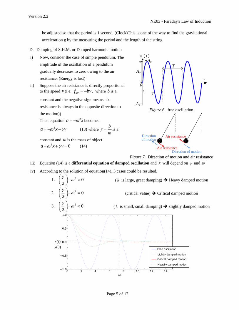
D. Damping of S.H.M. or Damped harmonic motion

i) Now, consider the case of simple pendulum. The

amplitude of the oscillation of a pendulum

gradually decreases to zero owing to the air

resistance. (Energy is lost)

ii) Suppose the air resistance is directly proportional

to the speed v (i.e. airf bv , where b is a

constant and the negative sign means air

resistance is always in the opposite direction to

the motion))

Then equation 2a x becomes

2a x v (13) where b

m is a

constant and m is the mass of object 2 0a x v (14)

x

Ao

t

t )(

0

+Ao

-Ao

T

T

Figure 6. free oscillation

Air resistance

Direction of motion

Direction of motion

Air resistance

Figure 7. Direction of motion and air resistance

iii) Equation (14) is a differential equation of damped oscillation and x will depend on and

iv) According to the solution of equation(14), 3 cases could be resulted.

1. 2 02

( k is large, great damping) Heavy damped motion

2. 2 02

(critical value) Critical damped motion

3. 2 02

( k is small, small damping) slightly damped motion

( )

(0)

x t

xFree oscillation

Lightly damped motion

Critical damped motion

Heavily damped motion

Version 2.2


Page 6 of 12

Figure 8. Amplitude ratio of free oscillation and different damped motion

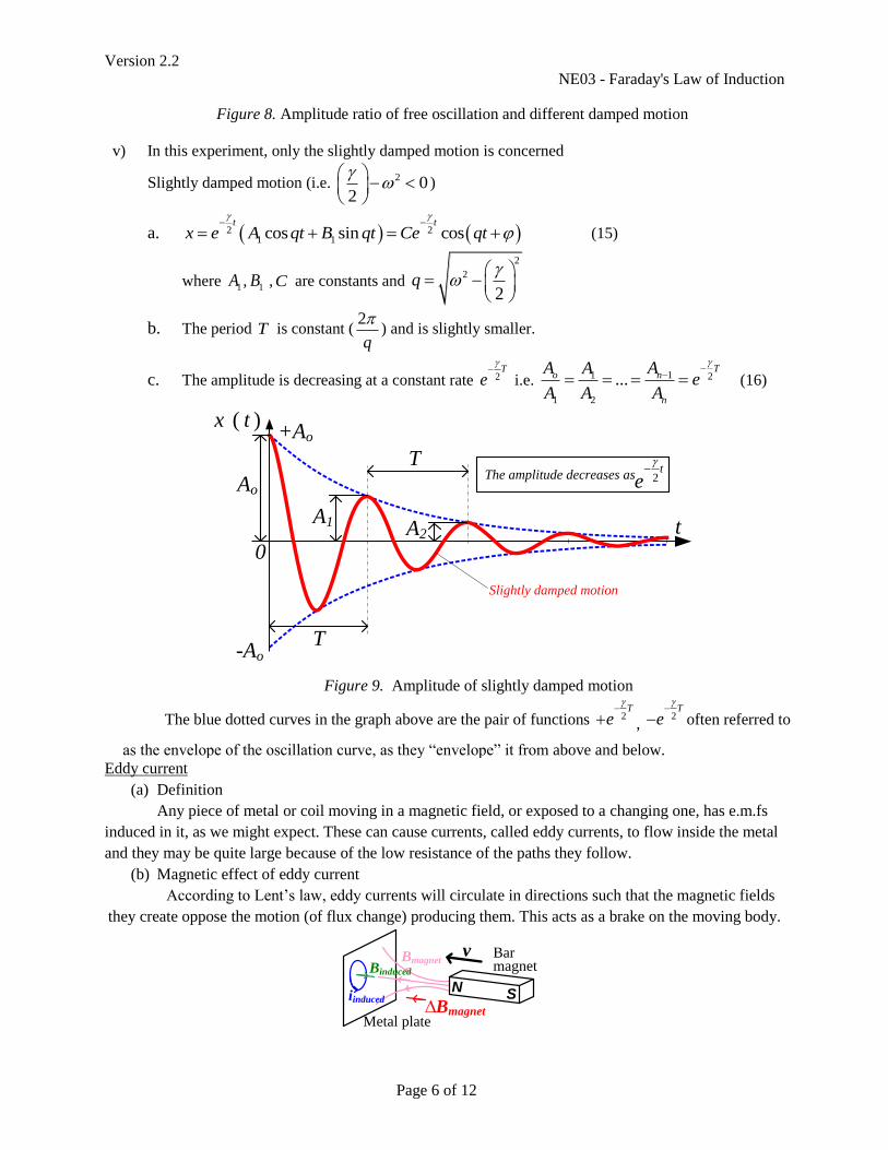
v) In this experiment, only the slightly damped motion is concerned

Slightly damped motion (i.e. 2 0

2

)

a. 2 21 1cos sin cos

t t

x e A qt B qt Ce qt

(15)

where 1A , 1B , C are constants and

2

2

2q

b. The period T is constant (2

q

) and is slightly smaller.

c. The amplitude is decreasing at a constant rate 2T

e

i.e. 11 2

1 2

...T

o n

n

A AAe

A A A

(16)

Ao

T

t

0

A1 A2

T

Slightly damped motion

+Ao

-Ao

2t

e

The amplitude decreases as

x t )(

Figure 9. Amplitude of slightly damped motion

The blue dotted curves in the graph above are the pair of functions 2T

e

, 2

T

e

often referred to

as the envelope of the oscillation curve, as they “envelope” it from above and below.

Eddy current

(a) Definition

Any piece of metal or coil moving in a magnetic field, or exposed to a changing one, has e.m.fs

induced in it, as we might expect. These can cause currents, called eddy currents, to flow inside the metal

and they may be quite large because of the low resistance of the paths they follow.

(b) Magnetic effect of eddy current

According to Lent’s law, eddy currents will circulate in directions such that the magnetic fields

they create oppose the motion (of flux change) producing them. This acts as a brake on the moving body.

Metal plate

NS

Bar magnet

vBmagnet

∆Bmagnet

Binduced

iinduced

Version 2.2


Page 7 of 12

Figure 10. Eddy current in a piece of metal plate

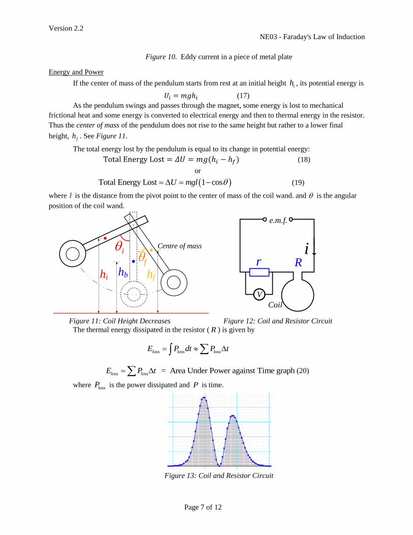
Energy and Power

If the center of mass of the pendulum starts from rest at an initial height ih , its potential energy is

𝑈𝑖 = 𝑚𝑔ℎ𝑖 (17)

As the pendulum swings and passes through the magnet, some energy is lost to mechanical

frictional heat and some energy is converted to electrical energy and then to thermal energy in the resistor.

Thus the center of mass of the pendulum does not rise to the same height but rather to a lower final

height, fh . See Figure 11.

The total energy lost by the pendulum is equal to its change in potential energy:

Total Energy Lost = 𝛥𝑈 = 𝑚𝑔(ℎ𝑖 − ℎ𝑓) (18)

or

Total Energy Lost 1 cosU mgl (19)

where l is the distance from the pivot point to the center of mass of the coil wand. and is the angular

position of the coil wand.

hi hfhb

Centre of massi

f

ir R

V

Coil

e.m.f.

Figure 11: Coil Height Decreases Figure 12: Coil and Resistor Circuit

The thermal energy dissipated in the resistor ( R ) is given by

loss loss lossE P dt P t

= Area Under Power against Time graphloss lossE P t (20)

where lossP is the power dissipated and P is time.

Figure 13: Coil and Resistor Circuit

Version 2.2


Page 8 of 12

Consider the circuit as shown in Figure 12, rV is the potential difference (p.d.) across the resistor

( r ), i is the current through the coil, and R is the resistance of the coil. According to Kirchhoff loop rule

reads:

. . .e m f R rV V (21)

Because of energy conservation, . . .e m f R rP P P

2 2

. . .e m f outputP P i R i r

The p.d. across the resistor ( r ), rV , is measured by voltmeter; according to Ohm’s law,

rr

VV ir i

r

The power output of the circuit is given by 2

outputP i R r (22)

2

( )routput

VP R r

r

(23)

In this experiment, 1.9R and 4.7r

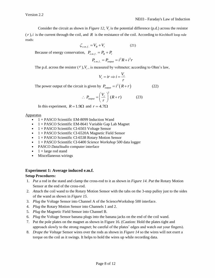
Apparatus

• 1 × PASCO Scientific EM-8099 Induction Wand

• 1 × PASCO Scientific EM-8641 Variable Gap Lab Magnet

• 1 × PASCO Scientific CI-6503 Voltage Sensor

• 1 × PASCO Scientific CI-6520A Magnetic Field Sensor

• 1 × PASCO Scientific CI-6538 Rotary Motion Sensor

• 1 × PASCO Scientific CI-6400 Science Workshop 500 data logger

• PASCO DataStudio computer interface

• 1 × large rod stand

• Miscellaneous wirings

Experiment 1: Average induced e.m.f.

Setup Procedures:

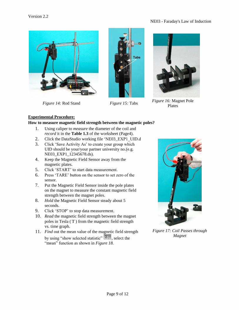
1. Put a rod in the stand and clamp the cross-rod to it as shown in Figure 14. Put the Rotary Motion

Sensor at the end of the cross-rod.

2. Attach the coil wand to the Rotary Motion Sensor with the tabs on the 3-step pulley just to the sides

of the wand as shown in Figure 15.

3. Plug the Voltage Sensor into Channel A of the ScienceWorkshop 500 interface.

4. Plug the Rotary Motion Sensor into Channels 1 and 2.

5. Plug the Magnetic Field Sensor into Channel B.

6. Plug the Voltage Sensor banana plugs into the banana jacks on the end of the coil wand.

7. Put the pole plates on the magnet as shown in Figure 16. (Caution: Hold the plates tight and

approach slowly to the strong magnet; be careful of the plates’ edges and watch out your fingers).

8. Drape the Voltage Sensor wires over the rods as shown in Figure 14 so the wires will not exert a

torque on the coil as it swings. It helps to hold the wires up while recording data.

Version 2.2


Page 9 of 12

Figure 14: Rod Stand Figure 15: Tabs Figure 16: Magnet Pole

Plates

Experimental Procedure:

How to measure magnetic field strength between the magnetic poles?

1. Using caliper to measure the diameter of the coil and

record it in the Table 1.3 of the worksheet (Page4).

2. Click the DataStudio working file ‘NE03_EXP1_UID.ds’

3. Click ‘Save Activity As’ to create your group which

UID should be your/your partner university no.(e.g.

NE03_EXP1_12345678.ds).

4. Keep the Magnetic Field Sensor away from the

magnetic plates.

5. Click ‘START’ to start data measurement.

6. Press ‘TARE’ button on the sensor to set zero of the

sensor.

7. Put the Magnetic Field Sensor inside the pole plates

on the magnet to measure the constant magnetic field

strength between the magnet poles.

8. Hold the Magnetic Field Sensor steady about 5

seconds.

9. Click ‘STOP’ to stop data measurement.

10. Read the magnetic field strength between the magnet

poles in Tesla ( T ) from the magnetic field strength

vs. time graph.

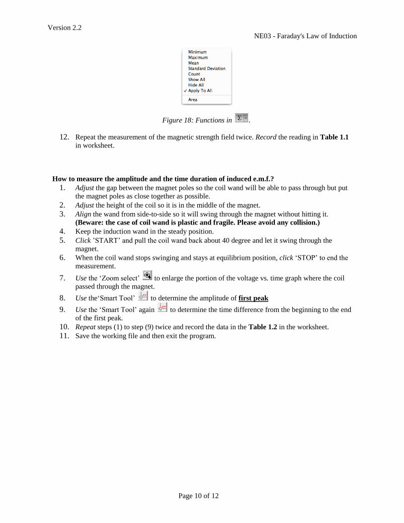
11. Find out the mean value of the magnetic field strength

by using “show selected statistic” , select the

“mean” function as shown in Figure 18.

Figure 17: Coil Passes through

Magnet

Version 2.2


Page 10 of 12

Figure 18: Functions in .

12. Repeat the measurement of the magnetic strength field twice. Record the reading in Table 1.1

in worksheet.

How to measure the amplitude and the time duration of induced e.m.f.?

1. Adjust the gap between the magnet poles so the coil wand will be able to pass through but put

the magnet poles as close together as possible.

2. Adjust the height of the coil so it is in the middle of the magnet.

3. Align the wand from side-to-side so it will swing through the magnet without hitting it.

(Beware: the case of coil wand is plastic and fragile. Please avoid any collision.)

4. Keep the induction wand in the steady position.

5. Click ’START’ and pull the coil wand back about 40 degree and let it swing through the

magnet.

6. When the coil wand stops swinging and stays at equilibrium position, click ‘STOP’ to end the

measurement.

7. Use the ‘Zoom select’ to enlarge the portion of the voltage vs. time graph where the coil

passed through the magnet.

8. Use the‘Smart Tool’ to determine the amplitude of first peak

9. Use the ‘Smart Tool’ again to determine the time difference from the beginning to the end

of the first peak.

10. Repeat steps (1) to step (9) twice and record the data in the Table 1.2 in the worksheet.

11. Save the working file and then exit the program.

Version 2.2


Page 11 of 12

Experiment 2: Lightly damped oscillation

Lightly damped oscillation due to friction and air resistance, eddy current and power loss of the

resistance in the coil

Experimental Procedure:

1. Open the DataStudio file called "NE03_EXP2_UID.ds".

2. Click ‘Save Activity As’ to create your group which UID should be your/your partner university

no.(e.g. NE03_EXP1_12345678.ds).

3. Now, the amount of energy lost to friction, air resistance and eddy current will be measured by

letting the pendulum swing with the coil connected in a complete circuit and presence of

magnetic field.

4. Connect the resistor with both plugs in the coil wand. This completes the series circuit of the resistor

and coil as shown in the Figure 12.

5. Click ’START’ with the coil at rest in its equilibrium position between the coils. Then rotate the

wand to an initial angle of 25 degrees and let it go. The angle is shown in digital meter

6. Click STOP ‘after the coil stops swinging.

7. Measure the initial angular position and angular position to which the pendulum firstly rises to

another side after it passes once through the magnet. Record it in Table 2.3 in the worksheet for the

1st trial measurement.

8. Calculate the initial and final heights by using the distance from the center of mass to the pivot and

the initial and final angular position in Table 2.2 in the worksheet. Record it in Table 2.3 in the

worksheet for the 1st trial measurement.

9. Calculate the total energy lost using equation (18).

10. Use the ‘Zoom select’ to enlarge the portion of the angular position vs. time graph where at least

five periods of curve is observed.

11. Use the ‘Smart Tool’ to determine the periods and amplitudes from the Angular position vs.

time graph. Record the data in Table 2.4.

Figure 23 Potential Energy vs. Time graph

12. Highlight both peaks on the power vs. time graph and find the area by using “show selected statistic”

, “Tick” the Area as shown in Figure 18. This area is the energy dissipated by the resistor.

Figure 24 Power vs. Time graph

13. Save the working file and then exit the program.

Version 2.2


Page 12 of 12

References:

Physical pendulum and Center of mass

1. http://hyperphysics.phy-astr.gsu.edu/hbase/pendp.html

2. Chapter 10, Physics for Scientists and Engineers with Modern Physics 8th Edition, John Jewett

and Raymond Serway

S.H.M.and Damped motions

3. http://hyperphysics.phy-astr.gsu.edu/hbase/shm.html#c1


and Raymond Serway

Magnetic field and Hall effect


and Raymond Serway

Faraday’s law and Eddy Current


and Raymond Serway

http://hyperphysics.phy-astr.gsu.edu/hbase/pendp.html

http://hyperphysics.phy-astr.gsu.edu/hbase/shm.html%23c1

Documents

Laboratory Manual NE03 - Faraday's Law of Induction ...physlab/fundamental/NE03_LM.pdf · NE03 - Faraday's Law of Induction Page 3 of 12 by their distances from a reference point