LabRAM User Guide - Trinity College, Dublin · Simple 14 Multiwindow 14 ... The instrument can be considered in four parts: 1. Lasers Œthe HeNe ... functions, see next page. MICROSCOPE

Page 1

LabRAM

User Guide

An Introduction to theSoftware and Hardware

v.01 11/2004

Page 2

Contents

Section 1 - Introduction to the LabRAM hardware and software 4

Introduction to the LabRAM hardware 5Introduction to the Labspec software 8The Hardware toolbar 9White light illumination � image acquisition 11

Section 2 - The LabSpec software for data acquisition 12

Acquiring a spectrum 13Real time spectrum adjustment 13Spectrum accumulation 13

Simple 14Multiwindow 14CREST 16Independent spectral windows 18

Acquiring mapped images and profiles 20Introduction 20Setting up a mapping/profiling experiment 21

Other acquisition functions 24Cosmic ray (random spike) removal 24Autosave 25Autofocus 26Autoexposure 27Extended white light imaging 28

Section 3 - The LabSpec software for data analysis 29

Data analysis functions 30Arithmetic 30Baseline correction 30Correction 31Profile 32Smoothing and filtering 33Fourier transformation 33Peak labelling and band fitting 34Band integration 36Object dimensions 37Object generation 38ASCII multi-file save 38Custom units 39

Page 3

Contents

Section 3 - The LabSpec software for data analysis (continued)

Analysing mapped images and profiles 40Analysing with cursors 40Analysing with models 41Displaying a mapped image of band position, width, area, etc 43

Data display functions 45View 45Colours/Axes 453D Option 46Scale 46

Other software functions 47Multi 47Axe + text 47Copy and paste 47XY(Z) stage display 47Units 48More objects 48Page set up (for printing) 49

Section 4 � A summary of software icons 50

A summary of software icons 51

Section 5 � Maintenance and calibration procedures 56

Calibrating the LabRAM 57Changing laser wavelength 59Calibrating the XY stage movement 60Calibrating the laser spot position 61Installing LabSpec software for data analysis 63

Section 6 � Contact details 66

Contact details for Horiba Jobin Yvon 67

Page 4

Section 1Introduction to the LabRAM Hardware and Software

Page 5

Introduction to the LabRAM Hardware

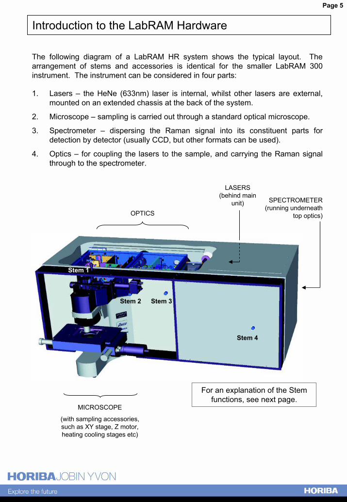
The following diagram of a LabRAM HR system shows the typical layout. The arrangement of stems and accessories is identical for the smaller LabRAM 300 instrument. The instrument can be considered in four parts:

1. Lasers � the HeNe (633nm) laser is internal, whilst other lasers are external, mounted on an extended chassis at the back of the system.

2. Microscope � sampling is carried out through a standard optical microscope.

3. Spectrometer � dispersing the Raman signal into its constituent parts for detection by detector (usually CCD, but other formats can be used).

4. Optics � for coupling the lasers to the sample, and carrying the Raman signal through to the spectrometer.

LASERS (behind main

unit)

Stem 2 Stem 3

Stem 4

Stem 1

SPECTROMETER (running underneath

top optics)OPTICS

For an explanation of the Stem functions, see next page.

MICROSCOPE

(with sampling accessories, such as XY stage, Z motor, heating cooling stages etc)

Page 6

Introduction to the LabRAM Hardware - continued

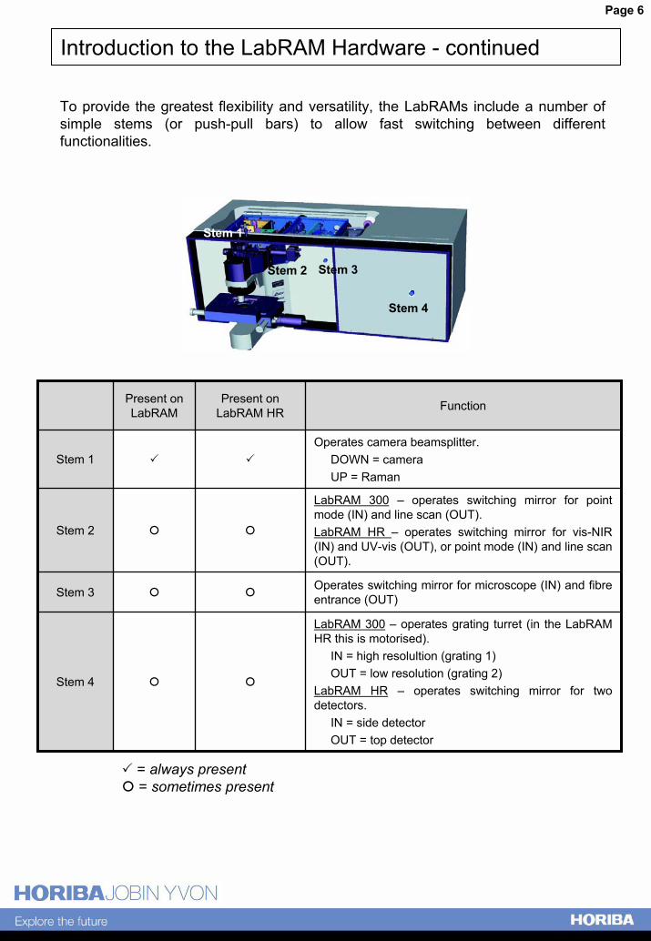
To provide the greatest flexibility and versatility, the LabRAMs include a number of simple stems (or push-pull bars) to allow fast switching between different functionalities.

Stem 2 Stem 3

Stem 4

Stem 1

LabRAM 300 � operates grating turret (in the LabRAM HR this is motorised).

IN = high resolultion (grating 1)OUT = low resolution (grating 2)

LabRAM HR � operates switching mirror for two detectors.

IN = side detectorOUT = top detector

!!Stem 4

Operates switching mirror for microscope (IN) and fibre entrance (OUT)!!Stem 3

LabRAM 300 � operates switching mirror for point mode (IN) and line scan (OUT).LabRAM HR � operates switching mirror for vis-NIR (IN) and UV-vis (OUT), or point mode (IN) and line scan (OUT).

!!Stem 2

Operates camera beamsplitter.DOWN = cameraUP = Raman

""Stem 1

FunctionPresent on LabRAM HR

Present on LabRAM

" = always present! = sometimes present

Page 7

Introduction to the LabRAM Hardware - continued

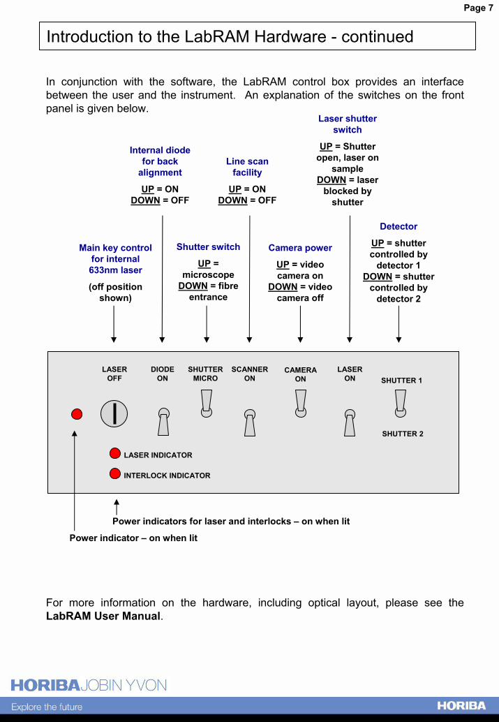
In conjunction with the software, the LabRAM control box provides an interface between the user and the instrument. An explanation of the switches on the front panel is given below.

LASER OFF

DIODE ON

SHUTTER MICRO

SCANNER ON

CAMERA ON

LASER ON SHUTTER 1

SHUTTER 2

LASER INDICATOR

INTERLOCK INDICATOR

Main key control for internal 633nm laser

(off position shown)

Shutter switch

UP = microscope

DOWN = fibre entrance

Camera power

UP = video camera on

DOWN = video camera off

Detector

UP = shutter controlled by

detector 1DOWN = shutter

controlled by detector 2

Internal diode for back

alignment

UP = ONDOWN = OFF

Line scan facility

UP = ONDOWN = OFF

Laser shutter switch

UP = Shutter open, laser on

sampleDOWN = laser

blocked by shutter

Power indicator � on when lit

Power indicators for laser and interlocks � on when lit

For more information on the hardware, including optical layout, please see the LabRAM User Manual.

Page 8

Introduction to the LabSpec Software

The LabSpec software provides a complete data acquisition and analysis package for use with the LabRAM.

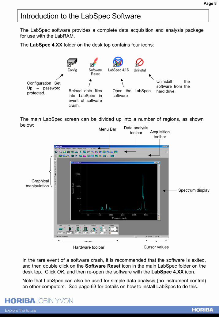
The LabSpec 4.XX folder on the desk top contains four icons:

Uninstall the software from the hard drive.

Configuration Set Up � password protected. Reload data files

into LabSpec in event of software crash.

Open the LabSpec software

The main LabSpec screen can be divided up into a number of regions, as shown below:

Graphical manipulation

Menu Bar Data analysis toolbar Acquisition

toolbar

Cursor valuesHardware toolbar

Spectrum display

In the rare event of a software crash, it is recommended that the software is exited, and then double click on the Software Reset icon in the main LabSpec folder on the desk top. Click OK, and then re-open the software with the LabSpec 4.XX icon.

Note that LabSpec can also be used for simple data analysis (no instrument control) on other computers. See page 63 for details on how to install LabSpec to do this.

Page 9

The Hardware Toolbar

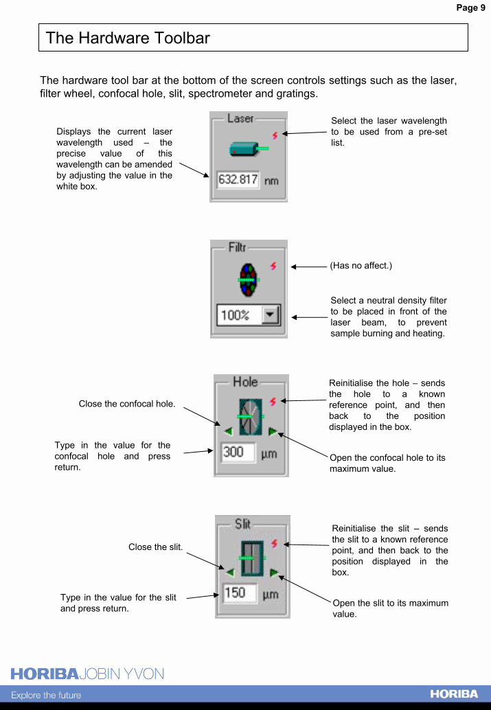
The hardware tool bar at the bottom of the screen controls settings such as the laser, filter wheel, confocal hole, slit, spectrometer and gratings.

Select the laser wavelength to be used from a pre-set list.

Displays the current laser wavelength used � the precise value of this wavelength can be amended by adjusting the value in the white box.

(Has no affect.)

Select a neutral density filter to be placed in front of the laser beam, to prevent sample burning and heating.

Reinitialise the hole � sends the hole to a known reference point, and then back to the position displayed in the box.

Close the confocal hole.

Type in the value for the confocal hole and press return.

Open the confocal hole to its maximum value.

Reinitialise the slit � sends the slit to a known reference point, and then back to the position displayed in the box.

Open the slit to its maximum value.

Close the slit.

Type in the value for the slit and press return.

Page 10

The Hardware Toolbar - continued

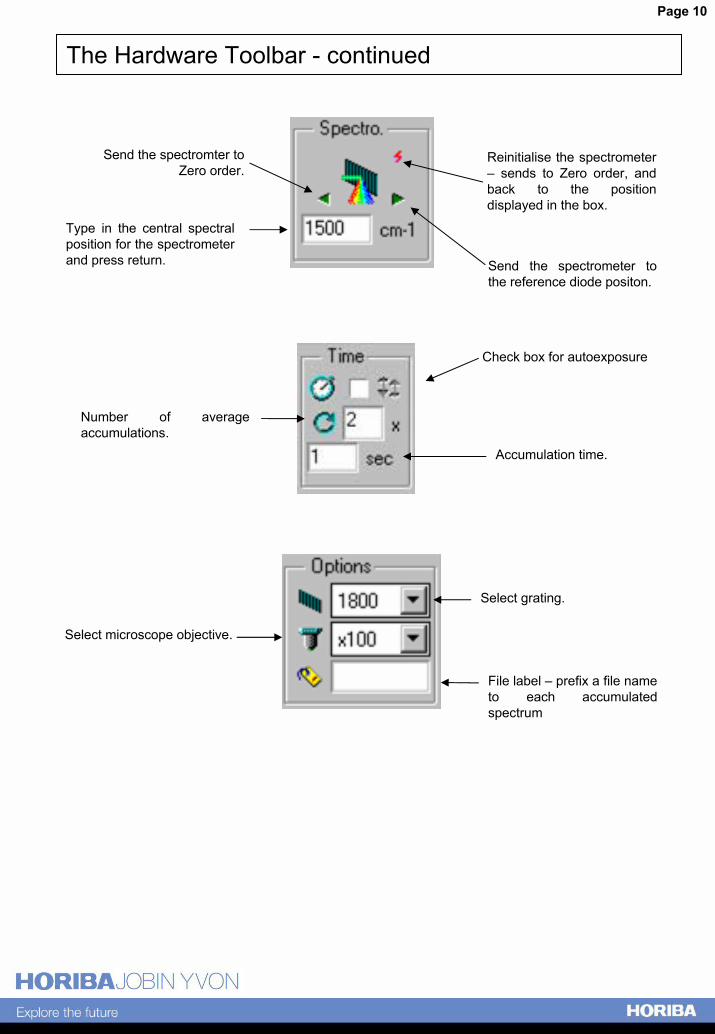
Reinitialise the spectrometer � sends to Zero order, and back to the position displayed in the box.

Send the spectrometer to the reference diode positon.

Send the spectromter to Zero order.

Type in the central spectral position for the spectrometer and press return.

Check box for autoexposure

Number of average accumulations.

Accumulation time.

Select grating.

Select microscope objective.

File label � prefix a file name to each accumulated spectrum

Page 11

White Light Illumination � Image Acquisition

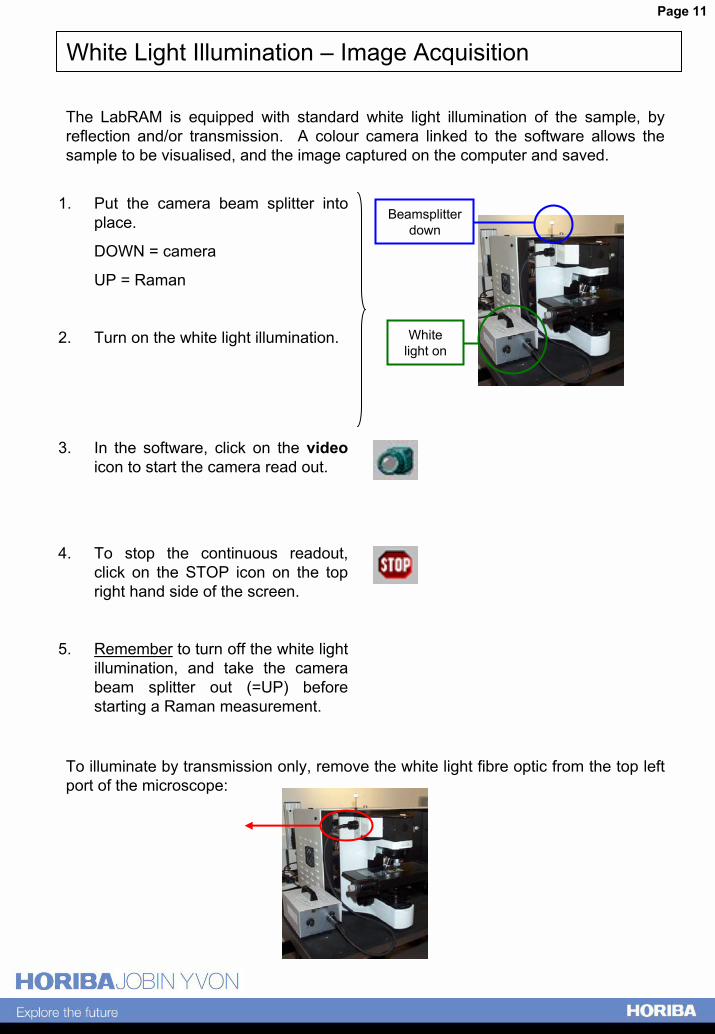
The LabRAM is equipped with standard white light illumination of the sample, by reflection and/or transmission. A colour camera linked to the software allows the sample to be visualised, and the image captured on the computer and saved.

1. Put the camera beam splitter into place.

DOWN = camera

UP = Raman

2. Turn on the white light illumination.

3. In the software, click on the video icon to start the camera read out.

4. To stop the continuous readout, click on the STOP icon on the top right hand side of the screen.

5. Remember to turn off the white light illumination, and take the camera beam splitter out (=UP) before starting a Raman measurement.

Beamsplitter down

White light on

To illuminate by transmission only, remove the white light fibre optic from the top left port of the microscope:

Page 12

Section 2The LabSpec Software for Data Acquisition

Page 13

Acquiring a spectrum

The LabSpec software provides the user with a number of methods for acquiring a single spectrum.

Real Time Spectrum Adjustment

This method is primarily designed for a fast display of the spectrum on screen corresponding to a single shot window. The update is continuous, providing a useful way of adjusting the focus position to maximise the Raman signal, and quickly monitoring the stability of the spectrum.

Each spectrum displayed replaces the previously displayed spectrum � there is no averaging or accumulation of the spectra, and no extended coverage possible. To do this you must use Spectrum Accumulation (see below).

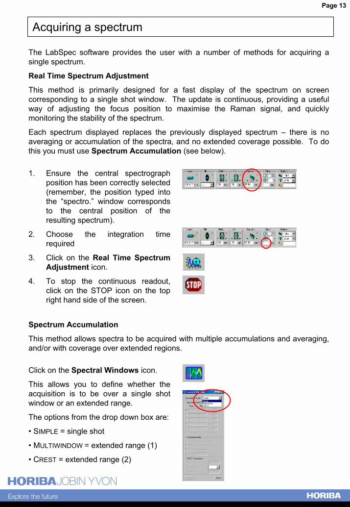
1. Ensure the central spectrograph position has been correctly selected (remember, the position typed into the �spectro.� window corresponds to the central position of the resulting spectrum).

2. Choose the integration time required

3. Click on the Real Time Spectrum Adjustment icon.

4. To stop the continuous readout, click on the STOP icon on the top right hand side of the screen.

Spectrum Accumulation

This method allows spectra to be acquired with multiple accumulations and averaging, and/or with coverage over extended regions.

Click on the Spectral Windows icon.

This allows you to define whether the acquisition is to be over a single shot window or an extended range.

The options from the drop down box are:

� SIMPLE = single shot

� MULTIWINDOW = extended range (1)

� CREST = extended range (2)

Page 14

Acquiring a spectrum - continued

Simple

This method allows a single shot spectrum to be acquired, with user defined integration time and averaging.

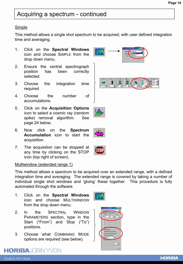
1. Click on the Spectral Windowsicon and choose SIMPLE from the drop down menu.

2. Ensure the central spectrograph position has been correctly selected.

3. Choose the integration time required

4. Choose the number of accumulations.

5. Click on the Acquisition Options icon to select a cosmic ray (random spike) removal algorithm. See page 24 below.

6. Now click on the Spectrum Accumulation icon to start the acquisition.

7. The acquisition can be stopped at any time by clicking on the STOP icon (top right of screen).

Multiwindow (extended range 1)

This method allows a spectrum to be acquired over an extended range, with a defined integration time and averaging. The extended range is covered by taking a number of individual single shot windows and �gluing� these together. This procedure is fully automated through the software.

1. Click on the Spectral Windowsicon and choose MULTIWINDOWfrom the drop down menu.

2. In the SPECTRAL WINDOWPARAMETERS section, type in the Start (�From�) and Stop (�To�) positions.

3. Choose what COMBINING MODEoptions are required (see below).

Page 15


4. Select the integration time and number of accumulations from the tool bar at the bottom of the screen.


6. Click on the Spectrum Accumulation icon to start the acquisition.


COMBINING MODE

The basic operation of MULTIWINDOW acquisition involves the acquisition of a number of discrete spectral windows, covering the chosen extended range. In order to simplify the process, it is possible to instruct the software to combine the individual spectra automatically, resulting in just one spectrum over the chosen extended range.

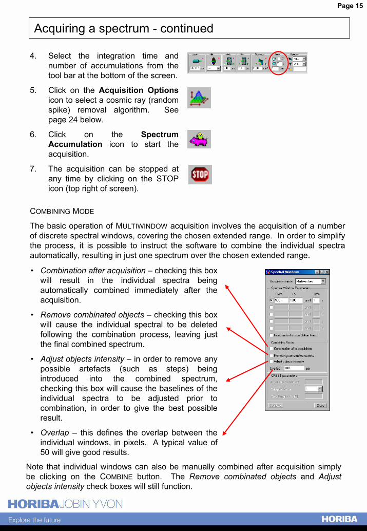
� Combination after acquisition � checking this box will result in the individual spectra being automatically combined immediately after the acquisition.

� Remove combinated objects � checking this box will cause the individual spectral to be deleted following the combination process, leaving just the final combined spectrum.

� Adjust objects intensity � in order to remove any possible artefacts (such as steps) being introduced into the combined spectrum, checking this box will cause the baselines of the individual spectra to be adjusted prior to combination, in order to give the best possible result.

� Overlap � this defines the overlap between the individual windows, in pixels. A typical value of 50 will give good results.

Note that individual windows can also be manually combined after acquisition simply be clicking on the COMBINE button. The Remove combinated objects and Adjust objects intensity check boxes will still function.

Page 16


CREST (extended range 1)

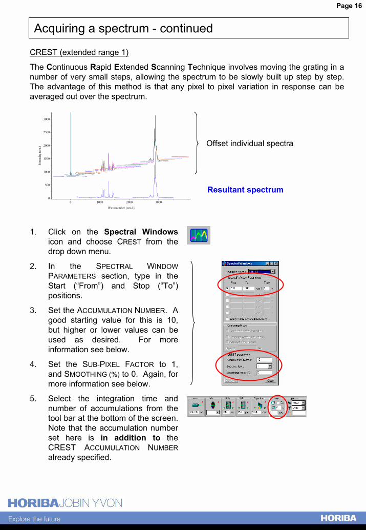
The Continuous Rapid Extended Scanning Technique involves moving the grating in a number of very small steps, allowing the spectrum to be slowly built up step by step. The advantage of this method is that any pixel to pixel variation in response can be averaged out over the spectrum.

3000

2500

2000

1500

1000

500

0

Inte

nsity

(a.u

.)

0 1000 2000 3000

Wavenumber (cm-1)

Offset individual spectra

Resultant spectrum

1. Click on the Spectral Windowsicon and choose CREST from the drop down menu.

2. In the SPECTRAL WINDOWPARAMETERS section, type in the Start (�From�) and Stop (�To�) positions.

3. Set the ACCUMULATION NUMBER. A good starting value for this is 10, but higher or lower values can be used as desired. For more information see below.

4. Set the SUB-PIXEL FACTOR to 1, and SMOOTHING (%) to 0. Again, for more information see below.

5. Select the integration time and number of accumulations from the tool bar at the bottom of the screen. Note that the accumulation number set here is in addition to the CREST ACCUMULATION NUMBERalready specified.

Page 17



7. Click on the Spectrum Accumulation icon to start the acquisition.


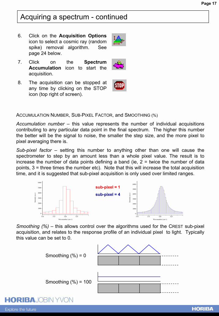
ACCUMULATION NUMBER, SUB-PIXEL FACTOR, and SMOOTHING (%)

Accumulation number � this value represents the number of individual acquisitions contributing to any particular data point in the final spectrum. The higher this number the better will be the signal to noise, the smaller the step size, and the more pixel to pixel averaging there is.

Sub-pixel factor � setting this number to anything other than one will cause the spectrometer to step by an amount less than a whole pixel value. The result is to increase the number of data points defining a band (ie, 2 = twice the number of data points, 3 = three times the number etc). Note that this will increase the total acquisition time, and it is suggested that sub-pixel acquisition is only used over limited ranges.

Smoothing (%) � this allows control over the algorithms used for the CREST sub-pixel acquisition, and relates to the response profile of an individual pixel to light. Typically this value can be set to 0.

Smoothing (%) = 0

Smoothing (%) = 100

6000

5000

4000

3000

2000

1000

0

Inte

nsity

(a.u

.)

510 515 520 525

Wavenumber (cm-1)

6000

5000

4000

3000

2000

1000

0

Inte

nsity

(a.u

.)

510 515 520 525

Wavenumber (cm-1)

sub-pixel = 1

sub-pixel = 4

Page 18


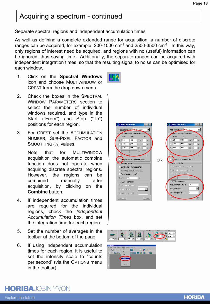
Separate spectral regions and independent accumulation times

As well as defining a complete extended range for acquisition, a number of discrete ranges can be acquired, for example, 200-1000 cm-1 and 2500-3500 cm-1. In this way, only regions of interest need be acquired, and regions with no (useful) information can be ignored, thus saving time. Additionally, the separate ranges can be acquired with independent integration times, so that the resulting signal to noise can be optimised for each window.

1. Click on the Spectral Windowsicon and choose MULTIWINDOW or CREST from the drop down menu.

2. Check the boxes in the SPECTRAL WINDOW PARAMETERS section to select the number of individual windows required, and type in the Start (�From�) and Stop (�To�) positions for each region.

3. For CREST set the ACCUMULATION NUMBER, SUB-PIXEL FACTOR and SMOOTHING (%) values.

Note that for MULTIWINDOWacquisition the automatic combine function does not operate when acquiring discrete spectral regions. However, the regions can be combined manually after acquisition, by clicking on the Combine button.

4. If independent accumulation times are required for the individual regions, check the Independent Accumulation Times box, and set the integration time for each region.

5. Set the number of averages in the toolbar at the bottom of the page.

6. If using independent accumulation times for each region, it is useful to set the intensity scale to �counts per second� (via the OPTIONS menu in the toolbar).

OR

Page 19



8. Click on the Spectral Accumulation icon to start the acquisition.


Note that the automatic combine function does not operate when acquiring discrete spectral regions by MULTIWINDOW, but the regions can be combined manually after acquisition.

For other acquisition functions which can be used in conjunction with those discussed here, please see the Other Acquisition Functions section on page 24.

Page 20

Acquiring Mapped Images and Profiles

Introduction

With suitable accessories on the LabRAM, it is possible to acquire XY mapped images, and line (X or Y), depth (Z), time and temperature profiles.

The principal of these measurements involves acquiring an array (2D or 1D) of spectra, with each spectrum acquired with a particular varied parameter (for example, position, or time).

Variation Description Hardware requirement

X and Y position map motorised XY stage

X or Y position line profile motorised XY stage

Z position depth or Z profile motorised Z stage/piezo

X, Y and Z position volume motorised XY and Z stage/piezo

Time time profile no accessory required

Temperature temperature profile heating/cooling sample stage

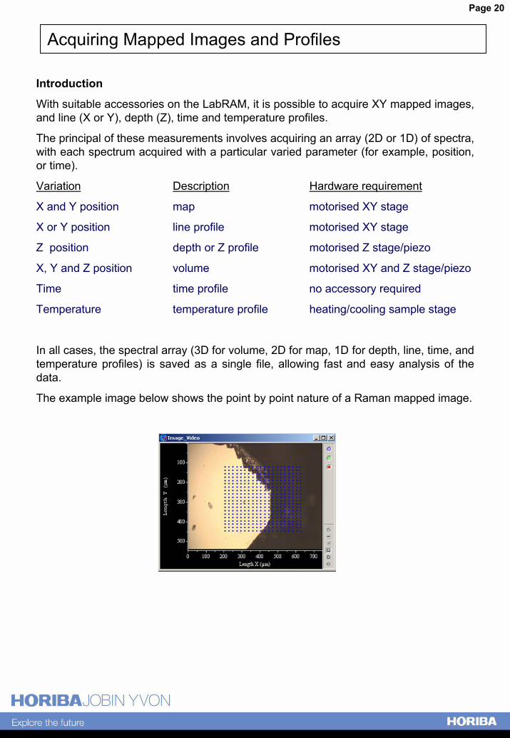
In all cases, the spectral array (3D for volume, 2D for map, 1D for depth, line, time, and temperature profiles) is saved as a single file, allowing fast and easy analysis of the data.

The example image below shows the point by point nature of a Raman mapped image.

Page 21

Acquiring Mapped Images and Profiles - continued

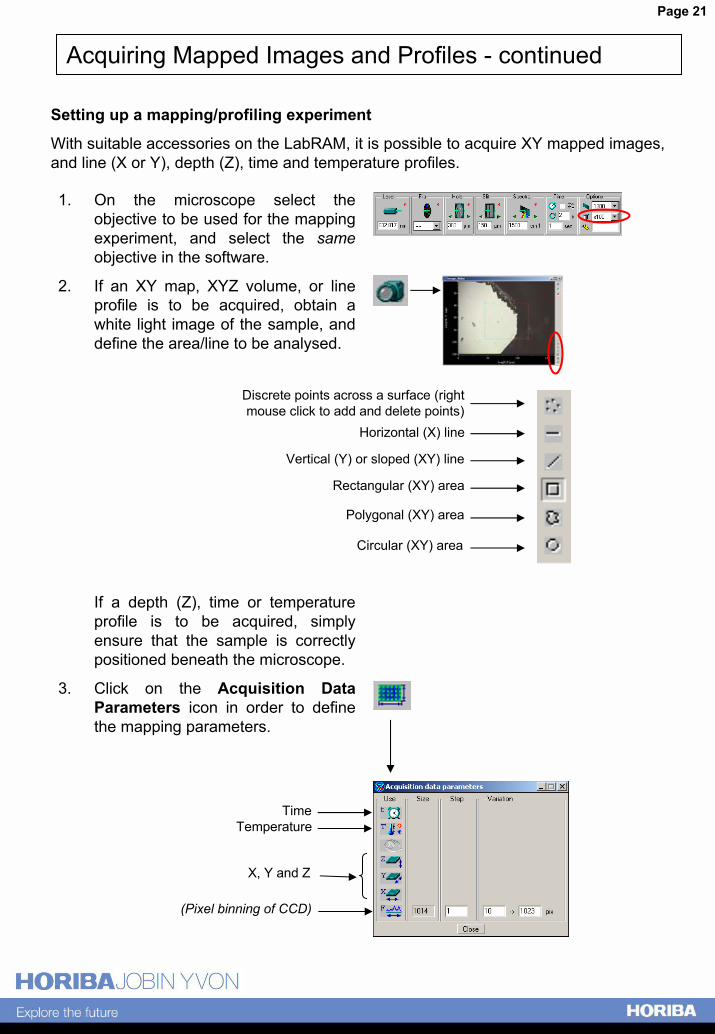
Setting up a mapping/profiling experiment

With suitable accessories on the LabRAM, it is possible to acquire XY mapped images, and line (X or Y), depth (Z), time and temperature profiles.

1. On the microscope select the objective to be used for the mapping experiment, and select the sameobjective in the software.

2. If an XY map, XYZ volume, or line profile is to be acquired, obtain a white light image of the sample, and define the area/line to be analysed.

If a depth (Z), time or temperature profile is to be acquired, simply ensure that the sample is correctly positioned beneath the microscope.

3. Click on the Acquisition Data Parameters icon in order to define the mapping parameters.

Discrete points across a surface (right mouse click to add and delete points)

Horizontal (X) line

Vertical (Y) or sloped (XY) line

Rectangular (XY) area

Polygonal (XY) area

Circular (XY) area

TimeTemperature

X, Y and Z

(Pixel binning of CCD)

Page 22


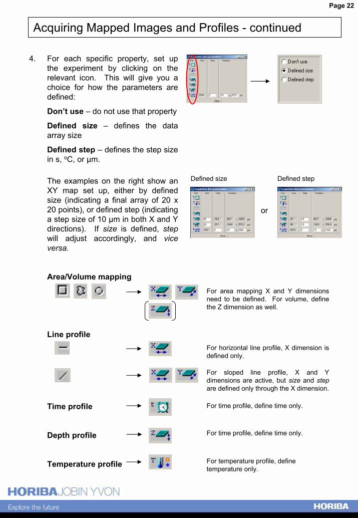
4. For each specific property, set up the experiment by clicking on the relevant icon. This will give you a choice for how the parameters are defined:

Don�t use � do not use that property

Defined size � defines the data array size

Defined step � defines the step size in s, oC, or µm.

The examples on the right show an XY map set up, either by defined size (indicating a final array of 20 x 20 points), or defined step (indicating a step size of 10 µm in both X and Y directions). If size is defined, stepwill adjust accordingly, and vice versa.

Area/Volume mapping

Line profile

Time profile

Depth profile

Temperature profile

Defined size Defined step

or

For area mapping X and Y dimensions need to be defined. For volume, define the Z dimension as well.

For horizontal line profile, X dimension is defined only.

For sloped line profile, X and Y dimensions are active, but size and stepare defined only through the X dimension.

For time profile, define time only.

For time profile, define time only.

For temperature profile, define temperature only.

Page 23


4. (continued)

Further specific details:

For time profiles, the step size is in seconds, and defines the time between the start of each acquisition. Note that the overall acquisition time per data point must be less than the step size.

For depth (Z) profiles, a negative number in the variation box implies moving the analysis point into the sample (ie, -20 ! 20 µm will move 20 µm below the start position, and step its way up to 20 µm above the start position). The start position is always defined as 0 µm.

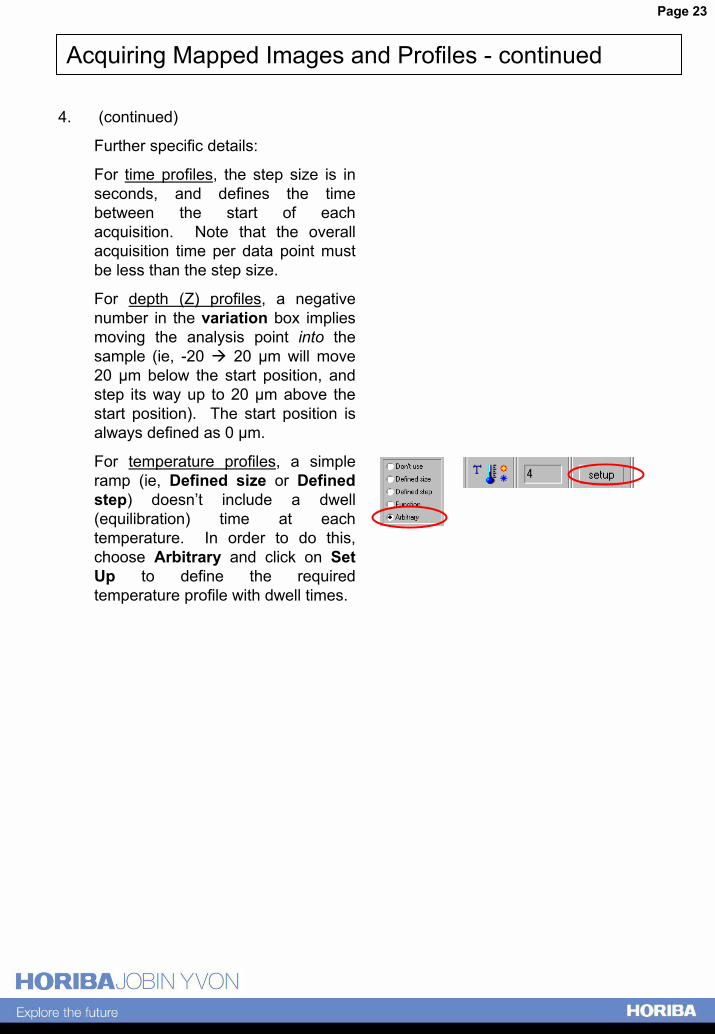
For temperature profiles, a simple ramp (ie, Defined size or Defined step) doesn�t include a dwell (equilibration) time at each temperature. In order to do this, choose Arbitrary and click on Set Up to define the required temperature profile with dwell times.

Page 24

Other Acquisition Functions

Cosmic Ray (Random Spike) Removal

The CCD detectors such as those used on the LabRAMs are sensitive to other forms of radiation, and in particular to random events known as �cosmic rays�. These can interfere with acquisition of spectra by registering as very sharp and strong bands in the spectrum.

Since the occurrence of a cosmic ray is random, it is extremely unlikely that a cosmic ray will occur in exactly the same part of the spectrum in two or more consecutive accumulations. Hence, it is possible to use a simple algorithm to detect random events in a spectrum (as opposed to constant features, such as a Raman peak).

In LabSpec there are two algorithms to choose from.

Multi accum This is the more robust algorithm, and works by comparing two (or more) accumulations within an acquisition. If a random cosmic ray spike is observed, the spike will be removed. For this algorithm to work, the accumulation number (averaging) must be set to greater than 2.

Single accum This algorithm attempts to locate a spike in a single accumulation acquisition (ie, accumulation number = 1), by analysing bands for sharpness (width) and intensity. This algorithm needs to be used with care, for very sharp Raman bands can easily be modified. However, the algorithm works very well when looking at broad features (such as Raman bands of amorphous materials, photoluminescence etc).

Note that both algorithms can be used for SIMPLE, MULTIWINDOW, and CREST, single point, mapping, profiling etc.

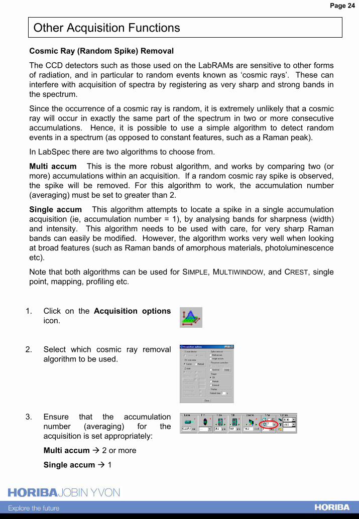
1. Click on the Acquisition optionsicon.

2. Select which cosmic ray removal algorithm to be used.

3. Ensure that the accumulation number (averaging) for the acquisition is set appropriately:

Multi accum ! 2 or more

Single accum ! 1

Page 25

Other Acquisition Functions - continued

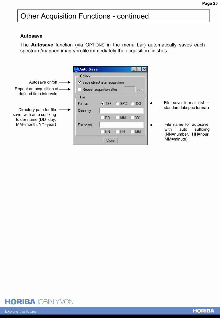
Autosave

The Autosave function (via OPTIONS in the menu bar) automatically saves each spectrum/mapped image/profile immediately the acquisition finishes.

Autosave on/offRepeat an acquisition at

defined time intervals.

File save format (tsf = standard labspec format)Directory path for file

save, with auto suffixing folder name (DD=day, MM=month, YY=year) File name for autosave,

with auto suffixing (NN=number, HH=hour, MM=minute).

Page 26


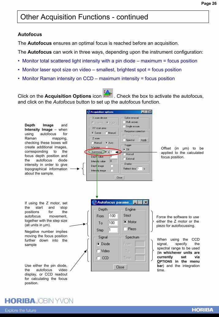
Autofocus

The Autofocus ensures an optimal focus is reached before an acquisition.

The Autofocus can work in three ways, depending upon the instrument configuration:

� Monitor total scattered light intensity with a pin diode � maximum = focus position

� Monitor laser spot size on video � smallest, brightest spot = focus position

� Monitor Raman intensity on CCD � maximum intensity = focus position

Click on the Acquisition Options icon . Check the box to activate the autofocus, and click on the Autofocus button to set up the autofocus function.

Depth Image and Intensity Image � when using autofocus for Raman mapping, checking these boxes will create additional images, corresponding to the focus depth position and the autofocus diode intensity in order to give topographical information about the sample.

Offset (in µm) to be applied to the calculated focus position.

Force the software to use either the Z motor or the piezo for autofocussing.

Use either the pin diode, the autofocus video display, or CCD readout for calculating the focus position.

If using the Z motor, set the start and stop positions for the autofocus movement, together with the step size (all units in µm).

Negative number implies moving the focus position further down into the sample

When using the CCD signal, specify the spectral range to be used (in whichever units are currently set via OPTIONS in the menu bar) and the integration time.

Page 27


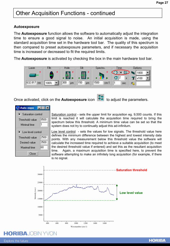
Autoexposure

The Autoexposure function allows the software to automatically adjust the integration time to ensure a good signal to noise. An initial acquisition is made, using the standard acquisition time set in the hardware tool bar. The quality of this spectrum is then compared to preset autoexposure parameters, and if necessary the acquisition time is increased or decreased to fit the required limits.

The Autoexposure is activated by checking the box in the main hardware tool bar.

Once activated, click on the Autoexposure icon to adjust the parameters.

Saturation control - sets the upper limit for acquisition eg. 9,500 counts. If this limit is reached it will calculate the acquisition time required to bring the spectrum below this threshold. A minimum time value can be set so that the system does not try to continually adjust this ad-infinitum.

Low level control - sets the values for low signals. The threshold value here defines the minimum difference between the highest and lowest intensity data points. With any measurement below this threshold value the software will calculate the increased time required to achieve a suitable acquisition (to meet the desired threshold value if entered) and set this as the resultant acquisition time. Again, a maximum acquisition time is specified here, to prevent the software attempting to make an infinitely long acquisition (for example, if there is no signal.

30000

25000

20000

15000

10000

5000

Inte

nsity

(a.u

.)

400 600 800 1000 1200 1400 1600

Wavenumber (cm-1)

Saturation threshold

Low level value

Page 28


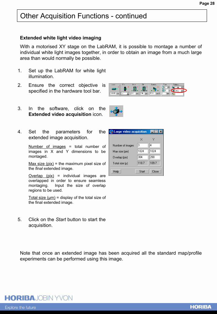
Extended white light video imaging

With a motorised XY stage on the LabRAM, it is possible to montage a number of individual white light images together, in order to obtain an image from a much large area than would normally be possible.

1. Set up the LabRAM for white light illumination.

2. Ensure the correct objective is specified in the hardware tool bar.

3. In the software, click on the Extended video acquisition icon.

4. Set the parameters for the extended image acquisition.

Number of images = total number of images in X and Y dimensions to be montaged.

Max size (pix) = the maximum pixel size of the final extended image.

Overlap (pix) = individual images are overlapped in order to ensure seamless montaging. Input the size of overlap regions to be used.

Total size (µm) = display of the total size of the final extended image.

5. Click on the Start button to start the acquisition.

Note that once an extended image has been acquired all the standard map/profile experiments can be performed using this image.

Page 29

Section 3The LabSpec Software for Data Analysis and Display

Page 30

Data Analysis Functions

The LabSpec software contains a wide range of data analysis functions, which are briefly described here.

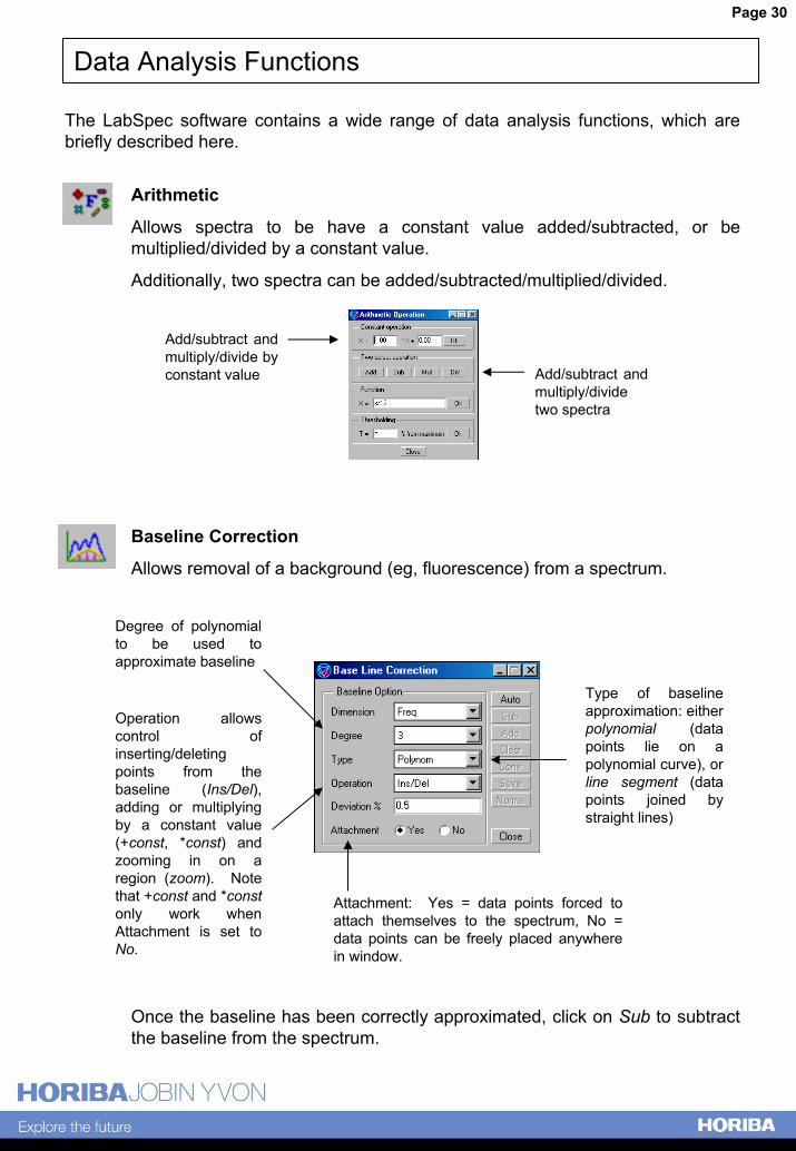
Arithmetic

Allows spectra to be have a constant value added/subtracted, or be multiplied/divided by a constant value.

Additionally, two spectra can be added/subtracted/multiplied/divided.

Baseline Correction

Allows removal of a background (eg, fluorescence) from a spectrum.

Once the baseline has been correctly approximated, click on Sub to subtract the baseline from the spectrum.

Add/subtract and multiply/divide by constant value Add/subtract and

multiply/divide two spectra

Degree of polynomial to be used to approximate baseline

Type of baseline approximation: either polynomial (data points lie on a polynomial curve), or line segment (data points joined by straight lines)

Attachment: Yes = data points forced to attach themselves to the spectrum, No = data points can be freely placed anywhere in window.

Operation allows control of inserting/deleting points from the baseline (Ins/Del), adding or multiplying by a constant value (+const, *const) and zooming in on a region (zoom). Note that +const and *constonly work when Attachment is set to No.

Page 31

Data Analysis Functions - continued

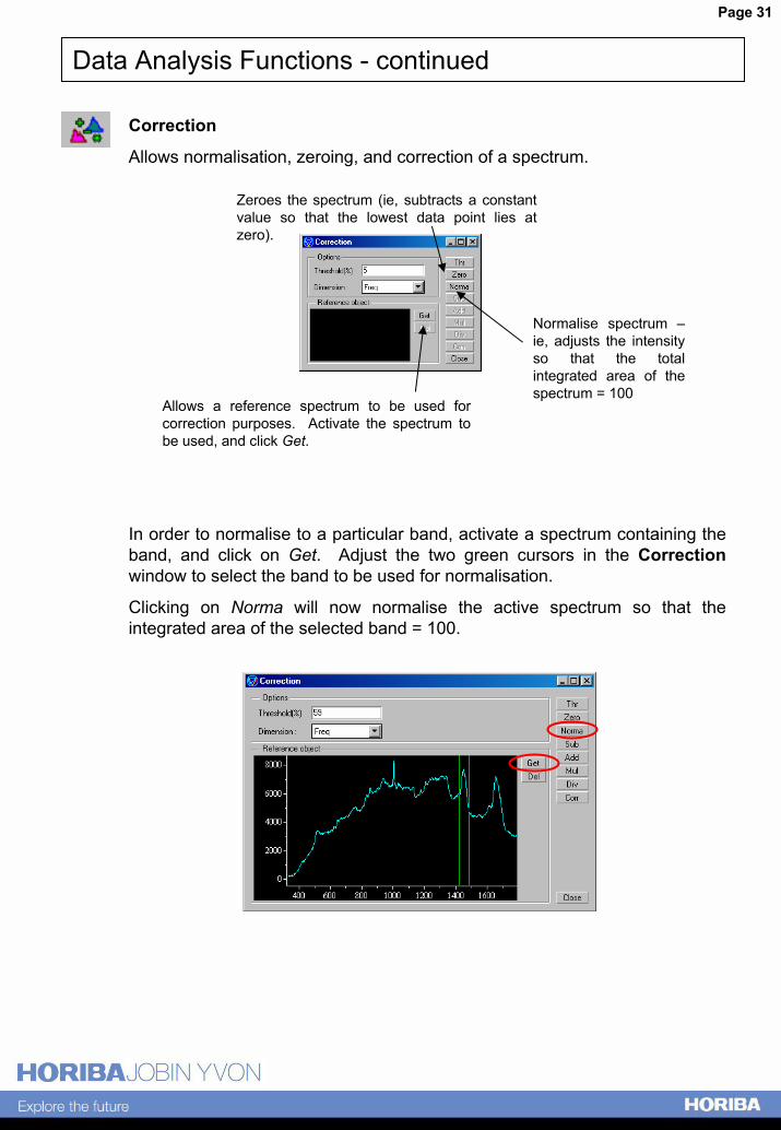
Zeroes the spectrum (ie, subtracts a constant value so that the lowest data point lies at zero).

Correction

Allows normalisation, zeroing, and correction of a spectrum.

In order to normalise to a particular band, activate a spectrum containing the band, and click on Get. Adjust the two green cursors in the Correctionwindow to select the band to be used for normalisation.

Clicking on Norma will now normalise the active spectrum so that the integrated area of the selected band = 100.

Normalise spectrum �ie, adjusts the intensity so that the total integrated area of the spectrum = 100

Allows a reference spectrum to be used for correction purposes. Activate the spectrum to be used, and click Get.

Page 32


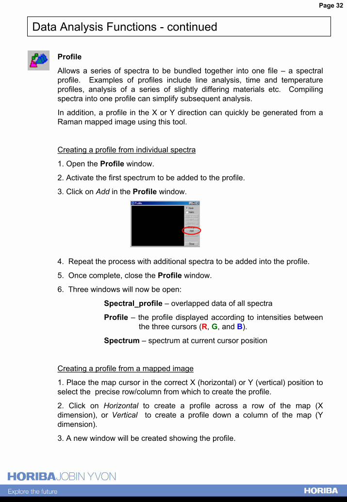
Profile

Allows a series of spectra to be bundled together into one file � a spectral profile. Examples of profiles include line analysis, time and temperature profiles, analysis of a series of slightly differing materials etc. Compiling spectra into one profile can simplify subsequent analysis.

In addition, a profile in the X or Y direction can quickly be generated from a Raman mapped image using this tool.

Creating a profile from individual spectra

1. Open the Profile window.

2. Activate the first spectrum to be added to the profile.

3. Click on Add in the Profile window.

4. Repeat the process with additional spectra to be added into the profile.

5. Once complete, close the Profile window.

6. Three windows will now be open:

Spectral_profile � overlapped data of all spectra

Profile � the profile displayed according to intensities between the three cursors (R, G, and B).

Spectrum � spectrum at current cursor position

Creating a profile from a mapped image

1. Place the map cursor in the correct X (horizontal) or Y (vertical) position to select the precise row/column from which to create the profile.

2. Click on Horizontal to create a profile across a row of the map (X dimension), or Vertical to create a profile down a column of the map (Y dimension).

3. A new window will be created showing the profile.

Page 33


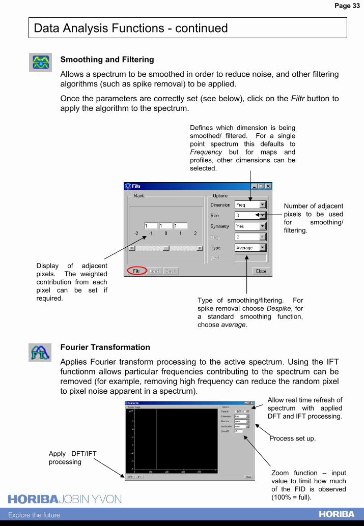
Smoothing and Filtering

Allows a spectrum to be smoothed in order to reduce noise, and other filtering algorithms (such as spike removal) to be applied.

Once the parameters are correctly set (see below), click on the Filtr button to apply the algorithm to the spectrum.

Defines which dimension is being smoothed/ filtered. For a single point spectrum this defaults to Frequency but for maps and profiles, other dimensions can be selected.

Number of adjacent pixels to be used for smoothing/ filtering.

Display of adjacent pixels. The weighted contribution from each pixel can be set if required. Type of smoothing/filtering. For

spike removal choose Despike, for a standard smoothing function, choose average.

Fourier Transformation

Applies Fourier transform processing to the active spectrum. Using the IFT functionm allows particular frequencies contributing to the spectrum can be removed (for example, removing high frequency can reduce the random pixel to pixel noise apparent in a spectrum).

Apply DFT/IFT processing

Process set up.

Allow real time refresh of spectrum with applied DFT and IFT processing.

Zoom function � input value to limit how much of the FID is observed (100% = full).

Page 34


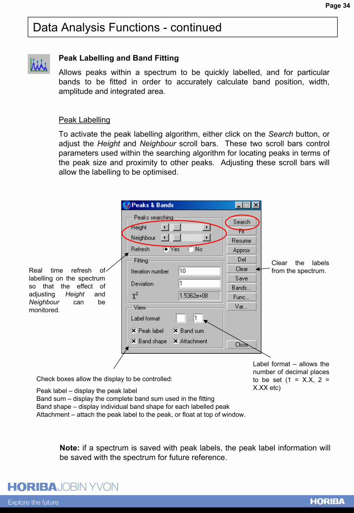
Peak Labelling and Band Fitting

Allows peaks within a spectrum to be quickly labelled, and for particular bands to be fitted in order to accurately calculate band position, width, amplitude and integrated area.

Peak Labelling

To activate the peak labelling algorithm, either click on the Search button, or adjust the Height and Neighbour scroll bars. These two scroll bars control parameters used within the searching algorithm for locating peaks in terms of the peak size and proximity to other peaks. Adjusting these scroll bars will allow the labelling to be optimised.

Real time refresh of labelling on the spectrum so that the effect of adjusting Height and Neighbour can be monitored.

Clear the labels from the spectrum.

Label format � allows the number of decimal places to be set (1 = X.X, 2 = X.XX etc)

Check boxes allow the display to be controlled:

Peak label � display the peak labelBand sum � display the complete band sum used in the fittingBand shape � display individual band shape for each labelled peakAttachment � attach the peak label to the peak, or float at top of window.

Note: if a spectrum is saved with peak labels, the peak label information will be saved with the spectrum for future reference.

Page 35


Peak Labelling and Band Fitting (continued)

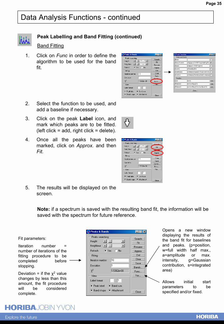
Band Fitting

1. Click on Func in order to define the algorithm to be used for the band fit.

2. Select the function to be used, and add a baseline if necessary.

3. Click on the peak Label icon, and mark which peaks are to be fitted. (left click = add, right click = delete).

4. Once all the peaks have been marked, click on Approx. and then Fit.

5. The results will be displayed on the screen.

Note: if a spectrum is saved with the resulting band fit, the information will be saved with the spectrum for future reference.

Opens a new window displaying the results of the band fit for baselines and peaks. (p=position, w=full width half max., a=amplitude or max. intensity, g=Gaussian contribution, s=integrated area)

Fit parameters:

Iteration number = number of iterations of the fitting procedure to be completed before stopping.

Deviation = if the χ2 value changes by less than this amount, the fit procedure will be considered complete.

Allows initial start parameters to be specified and/or fixed.

Page 36


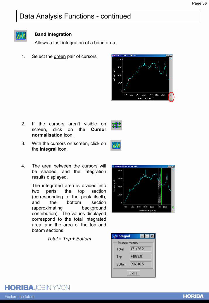
Band Integration

Allows a fast integration of a band area.

1. Select the green pair of cursors

2. If the cursors aren�t visible on screen, click on the Cursor normalisation icon.

3. With the cursors on screen, click on the Integral icon.

4. The area between the cursors will be shaded, and the integration results displayed.

The integrated area is divided into two parts; the top section (corresponding to the peak itself), and the bottom section (approximating background contribution). The values displayed correspond to the total integrated area, and the area of the top and botom sections:

Total = Top + Bottom

Page 37


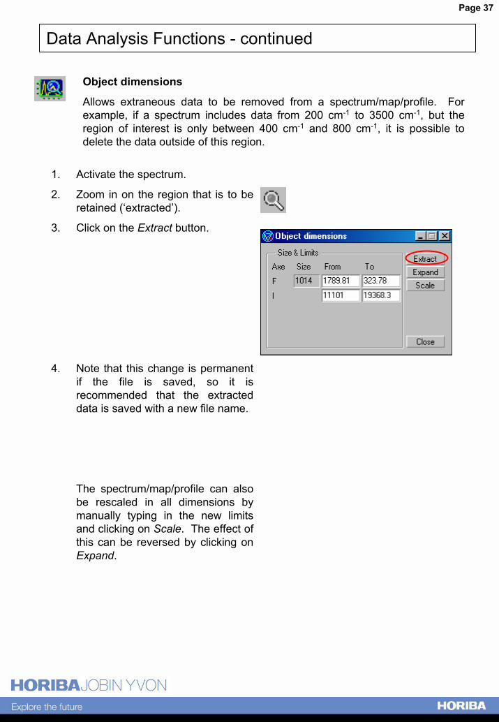
Object dimensions

Allows extraneous data to be removed from a spectrum/map/profile. For example, if a spectrum includes data from 200 cm-1 to 3500 cm-1, but the region of interest is only between 400 cm-1 and 800 cm-1, it is possible to delete the data outside of this region.

1. Activate the spectrum.

2. Zoom in on the region that is to be retained (�extracted�).

3. Click on the Extract button.

4. Note that this change is permanent if the file is saved, so it is recommended that the extracted data is saved with a new file name.

The spectrum/map/profile can also be rescaled in all dimensions by manually typing in the new limits and clicking on Scale. The effect of this can be reversed by clicking on Expand.

Page 38


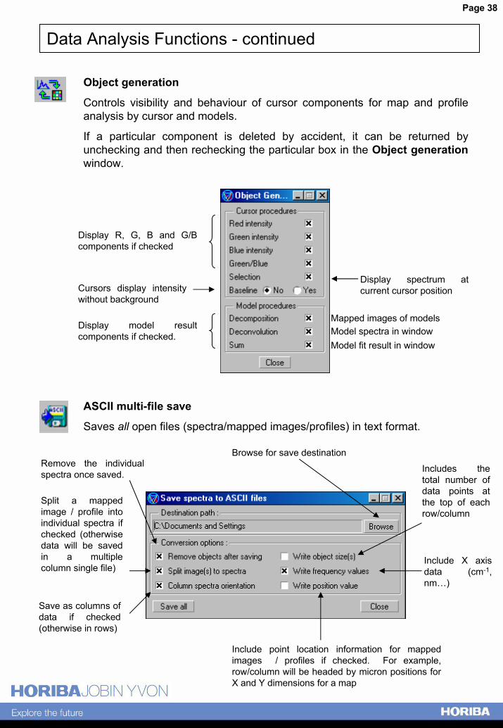
Object generation

Controls visibility and behaviour of cursor components for map and profile analysis by cursor and models.

If a particular component is deleted by accident, it can be returned by unchecking and then rechecking the particular box in the Object generationwindow.

Mapped images of models Model spectra in windowModel fit result in window

Display R, G, B and G/B components if checked

Display spectrum at current cursor positionCursors display intensity

without background

Display model result components if checked.

ASCII multi-file save

Saves all open files (spectra/mapped images/profiles) in text format.

Browse for save destinationRemove the individual spectra once saved. Includes the

total number of data points at the top of each row/column

Split a mapped image / profile into individual spectra if checked (otherwise data will be saved in a multiple column single file)

Include X axis data (cm-1, nm�)

Save as columns of data if checked (otherwise in rows)

Include point location information for mapped images / profiles if checked. For example, row/column will be headed by micron positions for X and Y dimensions for a map

Page 39


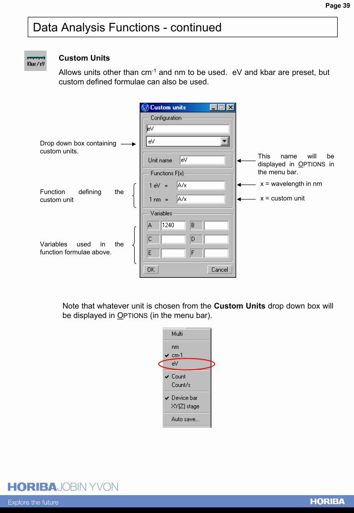
Custom Units

Allows units other than cm-1 and nm to be used. eV and kbar are preset, but custom defined formulae can also be used.

Drop down box containing custom units.

This name will be displayed in OPTIONS in the menu bar.

x = wavelength in nmFunction defining the custom unit x = custom unit

Variables used in the function formulae above.

Note that whatever unit is chosen from the Custom Units drop down box will be displayed in OPTIONS (in the menu bar).

Page 40

Analysing Mapped Images and Profiles

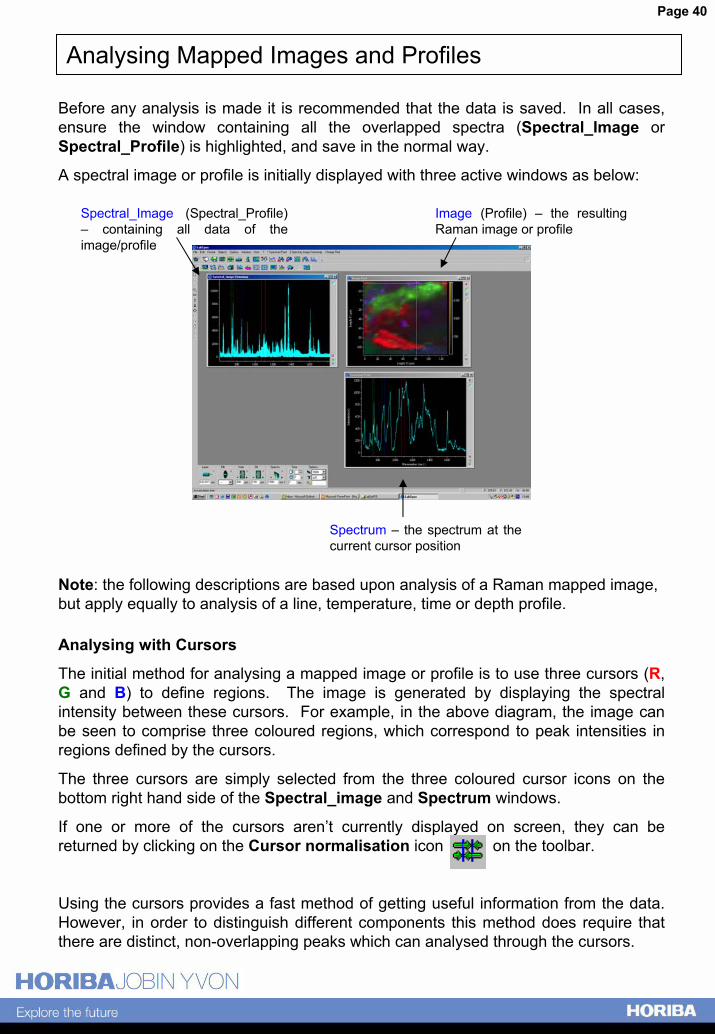
Before any analysis is made it is recommended that the data is saved. In all cases, ensure the window containing all the overlapped spectra (Spectral_Image or Spectral_Profile) is highlighted, and save in the normal way.

A spectral image or profile is initially displayed with three active windows as below:

Spectral_Image (Spectral_Profile) � containing all data of the image/profile

Spectrum � the spectrum at the current cursor position

Image (Profile) � the resulting Raman image or profile

Note: the following descriptions are based upon analysis of a Raman mapped image, but apply equally to analysis of a line, temperature, time or depth profile.

Analysing with Cursors

The initial method for analysing a mapped image or profile is to use three cursors (R, G and B) to define regions. The image is generated by displaying the spectral intensity between these cursors. For example, in the above diagram, the image can be seen to comprise three coloured regions, which correspond to peak intensities in regions defined by the cursors.

The three cursors are simply selected from the three coloured cursor icons on the bottom right hand side of the Spectral_image and Spectrum windows.

If one or more of the cursors aren�t currently displayed on screen, they can be returned by clicking on the Cursor normalisation icon on the toolbar.

Using the cursors provides a fast method of getting useful information from the data. However, in order to distinguish different components this method does require that there are distinct, non-overlapping peaks which can analysed through the cursors.

Page 41

Analysing Mapped Images and Profiles - continued

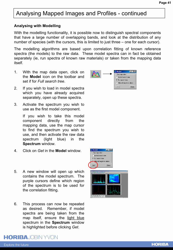
Analysing with Modelling

With the modelling functionality, it is possible now to distinguish spectral components that have a large number of overlapping bands, and look at the distribution of any number of species (with the cursors, this is limited to just three � one for each cursor).

The modelling algorithms are based upon correlation fitting of known reference spectra (the models) to the raw data. These model spectra can in fact be obtained separately (ie, run spectra of known raw materials) or taken from the mapping data itself.

1. With the map data open, click on the Model icon on the toolbar and set if for Full search tree.

2. If you wish to load in model spectra which you have already acquired separately, open up these spectra.

3. Activate the spectrum you wish to use as the first model component.

If you wish to take this model component directly from the mapping data, use the map cursor to find the spectrum you wish to use, and then activate the raw data spectrum (light blue) in the Spectrum window.

4. Click on Get in the Model window.

5. A new window will open up which contains the model spectrum. The purple cursors define which region of the spectrum is to be used for the correlation fitting.

6. This process can now be repeated as desired. Remember, if model spectra are being taken from the map itself, ensure the light bluespectrum in the Spectrum window is highlighted before clicking Get.

Page 42


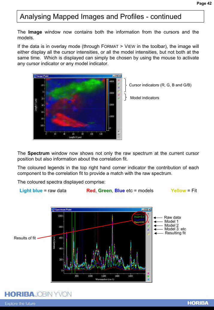
The Image window now contains both the information from the cursors and the models.

If the data is in overlay mode (through FORMAT > VIEW in the toolbar), the image will either display all the cursor intensities, or all the model intensities, but not both at the same time. Which is displayed can simply be chosen by using the mouse to activate any cursor indicator or any model indicator.

Cursor indicators (R, G, B and G/B)

Model indicators

The Spectrum window now shows not only the raw spectrum at the current cursor position but also information about the correlation fit.

The coloured legends in the top right hand corner indicator the contribution of each component to the correlation fit to provide a match with the raw spectrum.

The coloured spectra displayed comprise:

Light blue = raw data Red, Green, Blue etc = models Yellow = Fit

Raw dataModel 1Model 2Model 3 etcResulting fit

Results of fit

Page 43


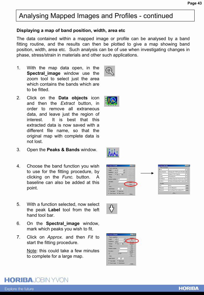
Displaying a map of band position, width, area etc

The data contained within a mapped image or profile can be analysed by a band fitting routine, and the results can then be plotted to give a map showing band position, width, area etc. Such analysis can be of use when investigating changes in phase, stress/strain in materials and other such applications.

1. With the map data open, in the Spectral_image window use the zoom tool to select just the area which contains the bands which are to be fitted.

2. Click on the Data objects icon and then the Extract button, in order to remove all extraneous data, and leave just the region of interest. It is best that this extracted data is now saved with a different file name, so that the original map with complete data is not lost.

3. Open the Peaks & Bands window.

4. Choose the band function you wish to use for the fitting procedure, by clicking on the Func. button. A baseline can also be added at this point.

5. With a function selected, now select the peak Label tool from the left hand tool bar.

6. On the Spectral_image window, mark which peaks you wish to fit.

7. Click on Approx. and then Fit to start the fitting procedure.

Note: this could take a few minutes to complete for a large map.

Page 44


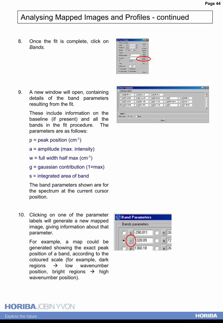
8. Once the fit is complete, click on Bands.

9. A new window will open, containing details of the band parameters resulting from the fit.

These include information on the baseline (if present) and all the bands in the fit procedure. The parameters are as follows:

p = peak position (cm-1)

a = amplitude (max. intensity)

w = full width half max (cm-1)

g = gaussian contribution (1=max)

s = integrated area of band

The band parameters shown are for the spectrum at the current cursor position.

10. Clicking on one of the parameter labels will generate a new mapped image, giving information about that parameter.

For example, a map could be generated showing the exact peak position of a band, according to the coloured scale (for example, dark regions ! low wavenumber position, bright regions ! high wavenumber position).

Page 45

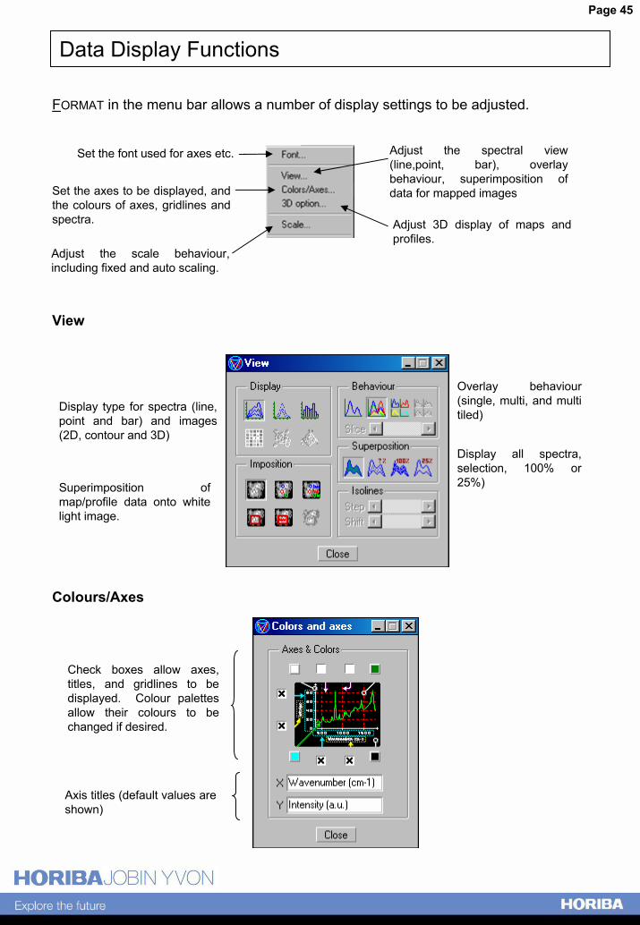
Data Display Functions

FORMAT in the menu bar allows a number of display settings to be adjusted.

Set the font used for axes etc. Adjust the spectral view (line,point, bar), overlay behaviour, superimposition of data for mapped imagesSet the axes to be displayed, and

the colours of axes, gridlines and spectra.

Adjust the scale behaviour, including fixed and auto scaling.

Adjust 3D display of maps and profiles.

View

Overlay behaviour (single, multi, and multi tiled)

Display type for spectra (line, point and bar) and images (2D, contour and 3D)

Display all spectra, selection, 100% or 25%)Superimposition of

map/profile data onto white light image.

Colours/Axes

Check boxes allow axes, titles, and gridlines to be displayed. Colour palettes allow their colours to be changed if desired.

Axis titles (default values are shown)

Page 46

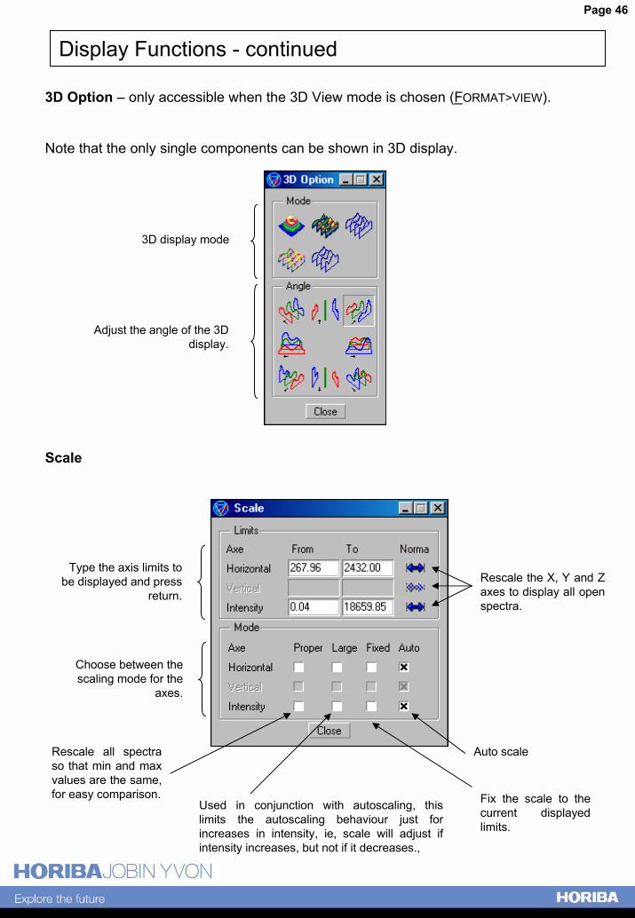
Display Functions - continued

3D Option � only accessible when the 3D View mode is chosen (FORMAT>VIEW).

Note that the only single components can be shown in 3D display.

3D display mode

Adjust the angle of the 3D display.

Scale

Auto scale

Type the axis limits to be displayed and press

return.Rescale the X, Y and Z axes to display all open spectra.

Choose between the scaling mode for the

axes.

Rescale all spectra so that min and max values are the same, for easy comparison. Fix the scale to the

current displayed limits.

Used in conjunction with autoscaling, this limits the autoscaling behaviour just for increases in intensity, ie, scale will adjust if intensity increases, but not if it decreases.,

Page 47

Other Functions

Multi

The Multi function (via OPTIONS in the menu bar) allows whatever process is performed on the active spectrum to be performed on all open spectrum.

For example, if a constant value is added to one spectrum, with Multi selected, all the open spectra will have that constant value added to them. This can be a useful way to save a number of files � with Multi selected, a save dialog window will appear for each open spectrum, in the order they are displayed in the Objects list.

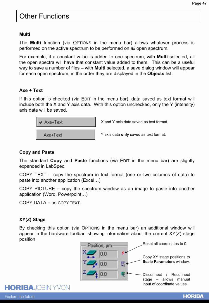
Axe + Text

If this option is checked (via EDIT in the menu bar), data saved as text format will include both the X and Y axis data. With this option unchecked, only the Y (intensity) axis data will be saved.

Copy and Paste

The standard Copy and Paste functions (via EDIT in the menu bar) are slightly expanded in LabSpec.

COPY TEXT = copy the spectrum in text format (one or two columns of data) to paste into another application (Excel�)

COPY PICTURE = copy the spectrum window as an image to paste into another application (Word, Powerpoint�)

COPY DATA = as COPY TEXT.

XY(Z) Stage

By checking this option (via OPTIONS in the menu bar) an additional window will appear in the hardware toolbar, showing information about the current XY(Z) stage position.

X and Y axis data saved as text format.

Y axis data only saved as text format.

Reset all coordinates to 0.

Disconnect / Reconnect stage � allows manual input of coordinate values.

Copy XY stage positions to Scale Parameters window.

Page 48

Other Functions - continued

Units

Units for the X axis can be specified as cm-1, nm and custom, and for the Y axis units can be specified as counts or counts/s. Via OPTIONS in the menu bar.

Custom units are defined and chosen using the Custom units icon in the toolbar � see page 39 for more details.

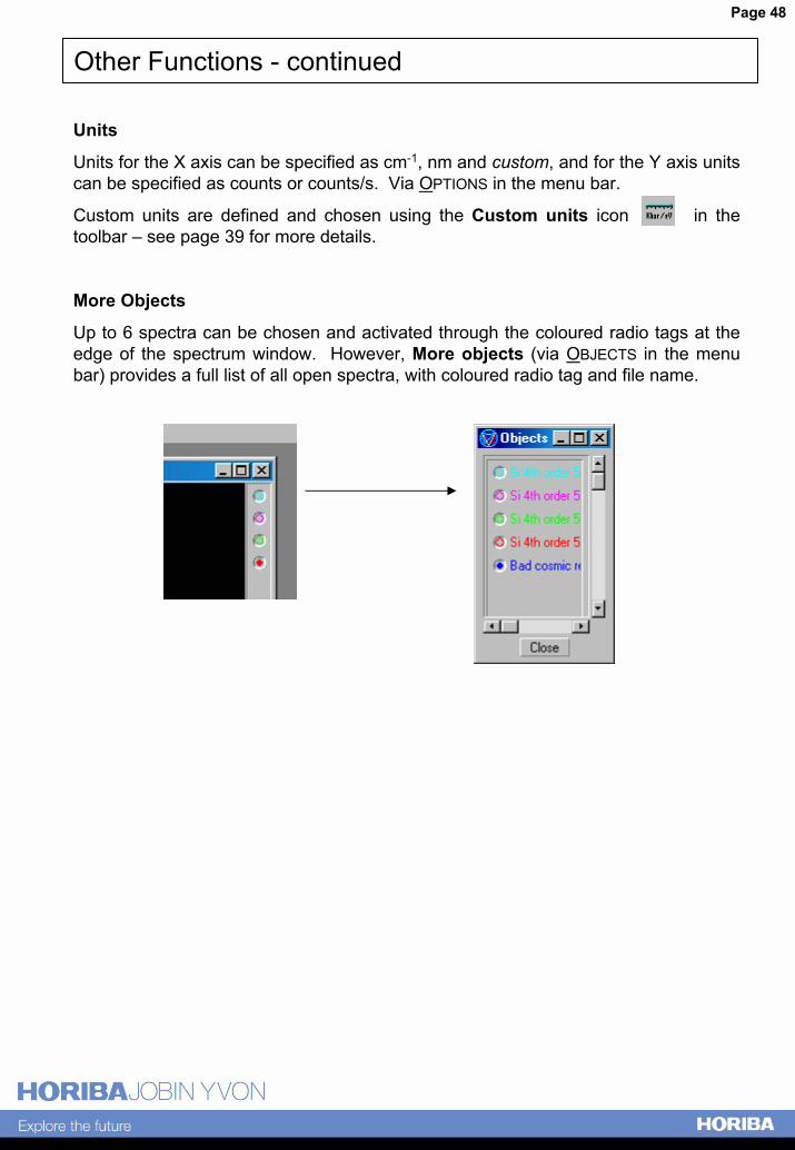
More Objects

Up to 6 spectra can be chosen and activated through the coloured radio tags at the edge of the spectrum window. However, More objects (via OBJECTS in the menu bar) provides a full list of all open spectra, with coloured radio tag and file name.

Page 49

Other Functions - continued

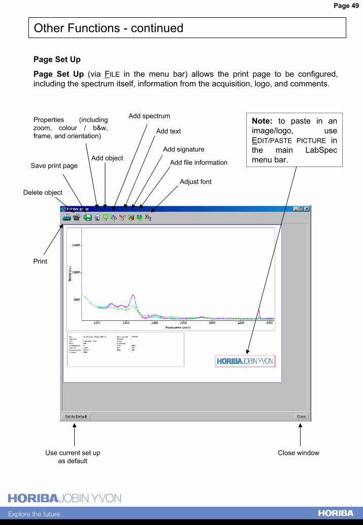
Page Set Up

Page Set Up (via FILE in the menu bar) allows the print page to be configured, including the spectrum itself, information from the acquisition, logo, and comments.

Delete object

Add object Add file information

Add spectrumProperties (including zoom, colour / b&w, frame, and orientation)

Note: to paste in an image/logo, use EDIT/PASTE PICTURE in the main LabSpec menu bar.

Add text

Add signature

Save print page

Adjust font

Print

Use current set up as default

Close window

Page 50

Section 4A Summary of Software Icons

Page 51

A Summary of Icons

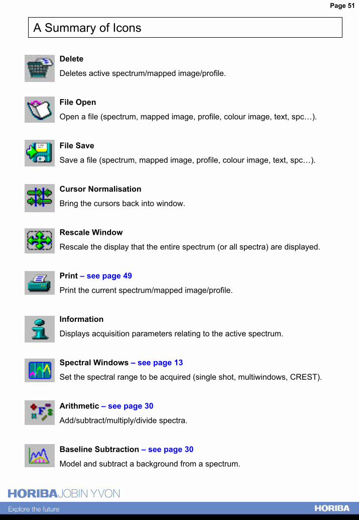
Delete

Deletes active spectrum/mapped image/profile.

File Open

Open a file (spectrum, mapped image, profile, colour image, text, spc�).

File Save

Save a file (spectrum, mapped image, profile, colour image, text, spc�).

Cursor Normalisation

Bring the cursors back into window.

Rescale Window

Rescale the display that the entire spectrum (or all spectra) are displayed.

Print � see page 49

Print the current spectrum/mapped image/profile.

Information

Displays acquisition parameters relating to the active spectrum.

Spectral Windows � see page 13

Set the spectral range to be acquired (single shot, multiwindows, CREST).

Arithmetic � see page 30

Add/subtract/multiply/divide spectra.

Baseline Subtraction � see page 30

Model and subtract a background from a spectrum.

Page 52

A Summary of Icons - continued

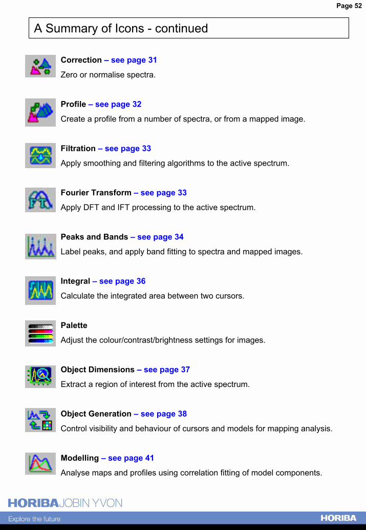
Correction � see page 31

Zero or normalise spectra.

Profile � see page 32

Create a profile from a number of spectra, or from a mapped image.

Filtration � see page 33

Apply smoothing and filtering algorithms to the active spectrum.

Fourier Transform � see page 33

Apply DFT and IFT processing to the active spectrum.

Peaks and Bands � see page 34

Label peaks, and apply band fitting to spectra and mapped images.

Integral � see page 36

Calculate the integrated area between two cursors.

Palette

Adjust the colour/contrast/brightness settings for images.

Object Dimensions � see page 37

Extract a region of interest from the active spectrum.

Object Generation � see page 38

Control visibility and behaviour of cursors and models for mapping analysis.

Modelling � see page 41

Analyse maps and profiles using correlation fitting of model components.

Page 53


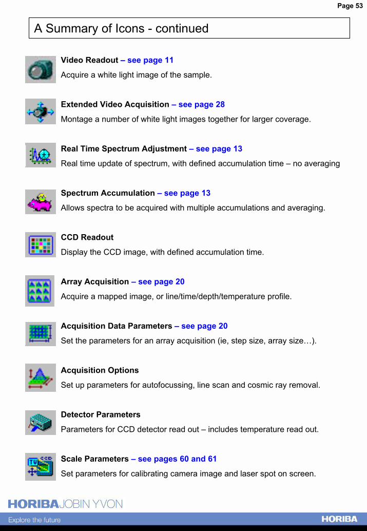
Video Readout � see page 11

Acquire a white light image of the sample.

Extended Video Acquisition � see page 28

Montage a number of white light images together for larger coverage.

Real Time Spectrum Adjustment � see page 13

Real time update of spectrum, with defined accumulation time � no averaging

Spectrum Accumulation � see page 13

Allows spectra to be acquired with multiple accumulations and averaging.

CCD Readout

Display the CCD image, with defined accumulation time.

Array Acquisition � see page 20

Acquire a mapped image, or line/time/depth/temperature profile.

Acquisition Data Parameters � see page 20

Set the parameters for an array acquisition (ie, step size, array size�).

Acquisition Options

Set up parameters for autofocussing, line scan and cosmic ray removal.

Detector Parameters

Parameters for CCD detector read out � includes temperature read out.

Scale Parameters � see pages 60 and 61

Set parameters for calibrating camera image and laser spot on screen.

Page 54


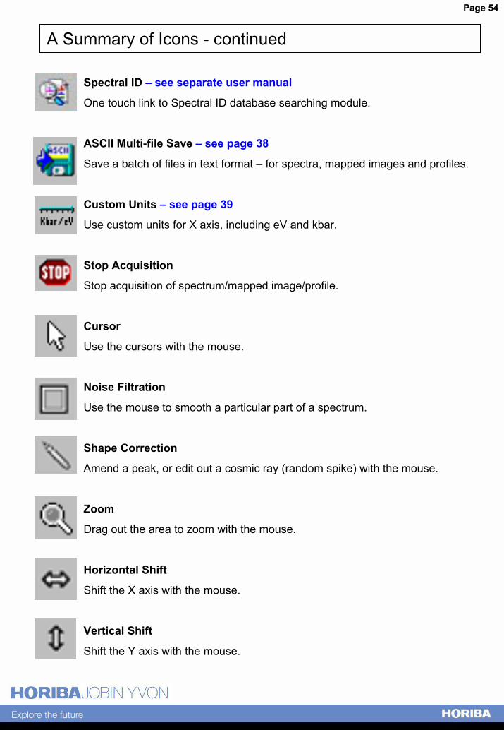
Spectral ID � see separate user manual

One touch link to Spectral ID database searching module.

ASCII Multi-file Save � see page 38

Save a batch of files in text format � for spectra, mapped images and profiles.

Custom Units � see page 39

Use custom units for X axis, including eV and kbar.

Stop Acquisition

Stop acquisition of spectrum/mapped image/profile.

Cursor

Use the cursors with the mouse.

Noise Filtration

Use the mouse to smooth a particular part of a spectrum.

Shape Correction

Amend a peak, or edit out a cosmic ray (random spike) with the mouse.

Zoom

Drag out the area to zoom with the mouse.

Horizontal Shift

Shift the X axis with the mouse.

Vertical Shift

Shift the Y axis with the mouse.

Page 55


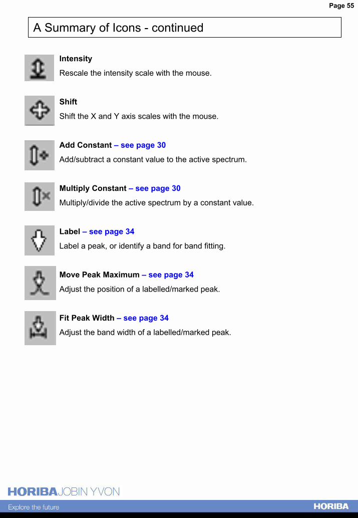
Intensity

Rescale the intensity scale with the mouse.

Shift

Shift the X and Y axis scales with the mouse.

Add Constant � see page 30

Add/subtract a constant value to the active spectrum.

Multiply Constant � see page 30

Multiply/divide the active spectrum by a constant value.

Label � see page 34

Label a peak, or identify a band for band fitting.

Move Peak Maximum � see page 34

Adjust the position of a labelled/marked peak.

Fit Peak Width � see page 34

Adjust the band width of a labelled/marked peak.

Page 56

Section 5Maintenance and Calibration Procedures

Page 57

Calibrating the LabRAM

Before acquiring a spectrum, the LabRAM needs to be calibrated. This is a simple procedure involving two software parameters

ZERO This is a number used to define the position of the zero order of the spectrograph and can be thought of as the number of motor steps to move away from a mechanical calibration sensor.

KOEFF This can be thought of as the number of nm moved per motor step.

Part 1 - Calibrating the Zero order position

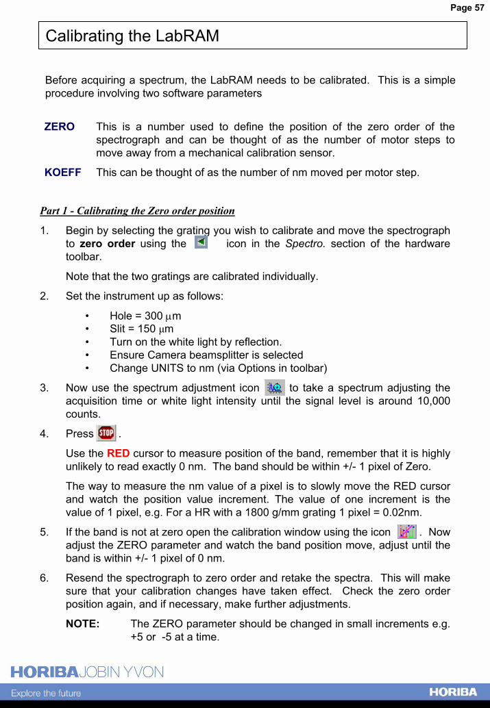
1. Begin by selecting the grating you wish to calibrate and move the spectrograph to zero order using the icon in the Spectro. section of the hardware toolbar.

Note that the two gratings are calibrated individually.

2. Set the instrument up as follows:

� Hole = 300 µm� Slit = 150 µm� Turn on the white light by reflection.� Ensure Camera beamsplitter is selected� Change UNITS to nm (via Options in toolbar)

3. Now use the spectrum adjustment icon to take a spectrum adjusting the acquisition time or white light intensity until the signal level is around 10,000 counts.

4. Press .

Use the RED cursor to measure position of the band, remember that it is highly unlikely to read exactly 0 nm. The band should be within +/- 1 pixel of Zero.

The way to measure the nm value of a pixel is to slowly move the RED cursor and watch the position value increment. The value of one increment is the value of 1 pixel, e.g. For a HR with a 1800 g/mm grating 1 pixel = 0.02nm.

5. If the band is not at zero open the calibration window using the icon . Now adjust the ZERO parameter and watch the band position move, adjust until the band is within +/- 1 pixel of 0 nm.

6. Resend the spectrograph to zero order and retake the spectra. This will make sure that your calibration changes have taken effect. Check the zero order position again, and if necessary, make further adjustments.

NOTE: The ZERO parameter should be changed in small increments e.g. +5 or -5 at a time.

Page 58

Calibrating the LabRAM - continued

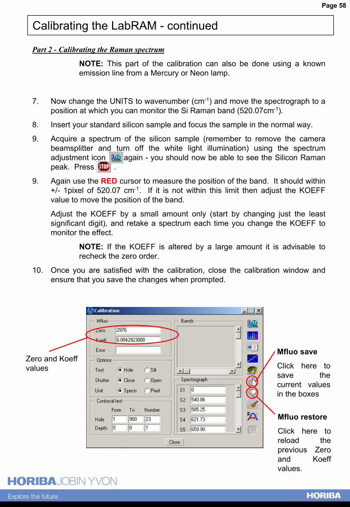
Part 2 - Calibrating the Raman spectrum

NOTE: This part of the calibration can also be done using a known emission line from a Mercury or Neon lamp.

7. Now change the UNITS to wavenumber (cm-1) and move the spectrograph to a position at which you can monitor the Si Raman band (520.07cm-1).

8. Insert your standard silicon sample and focus the sample in the normal way.

9. Acquire a spectrum of the silicon sample (remember to remove the camera beamsplitter and turn off the white light illumination) using the spectrum adjustment icon again - you should now be able to see the Silicon Raman peak. Press .

9. Again use the RED cursor to measure the position of the band. It should within +/- 1pixel of 520.07 cm-1. If it is not within this limit then adjust the KOEFF value to move the position of the band.

Adjust the KOEFF by a small amount only (start by changing just the least significant digit), and retake a spectrum each time you change the KOEFF to monitor the effect.

NOTE: If the KOEFF is altered by a large amount it is advisable to recheck the zero order.

10. Once you are satisfied with the calibration, close the calibration window and ensure that you save the changes when prompted.

Zero and Koeff values

Mfluo save

Click here to save the current values in the boxes

Mfluo restore

Click here to reload the previous Zero and Koeff values.

Page 59

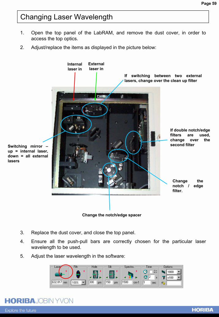
Changing Laser Wavelength

1. Open the top panel of the LabRAM, and remove the dust cover, in order to access the top optics.

2. Adjust/replace the items as displayed in the picture below:

3. Replace the dust cover, and close the top panel.

4. Ensure all the push-pull bars are correctly chosen for the particular laser wavelength to be used.

5. Adjust the laser wavelength in the software:

Internal laser in

External laser in

If switching between two external lasers, change over the clean up filter

Change the notch/edge spacer

If double notch/edge filters are used, change over the second filterSwitching mirror �

up = internal laser, down = all external lasers

Change the notch / edge filter.

Page 60

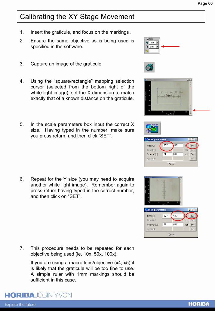
Calibrating the XY Stage Movement

1. Insert the graticule, and focus on the markings .

2. Ensure the same objective as is being used is specified in the software.

3. Capture an image of the graticule

4. Using the �square/rectangle� mapping selection cursor (selected from the bottom right of the white light image), set the X dimension to match exactly that of a known distance on the graticule.

5. In the scale parameters box input the correct X size. Having typed in the number, make sure you press return, and then click �SET�.

6. Repeat for the Y size (you may need to acquire another white light image). Remember again to press return having typed in the correct number, and then click on �SET�.

7. This procedure needs to be repeated for each objective being used (ie, 10x, 50x, 100x).

If you are using a macro lens/objective (x4, x5) it is likely that the graticule will be too fine to use. A simple ruler with 1mm markings should be sufficient in this case.

Page 61

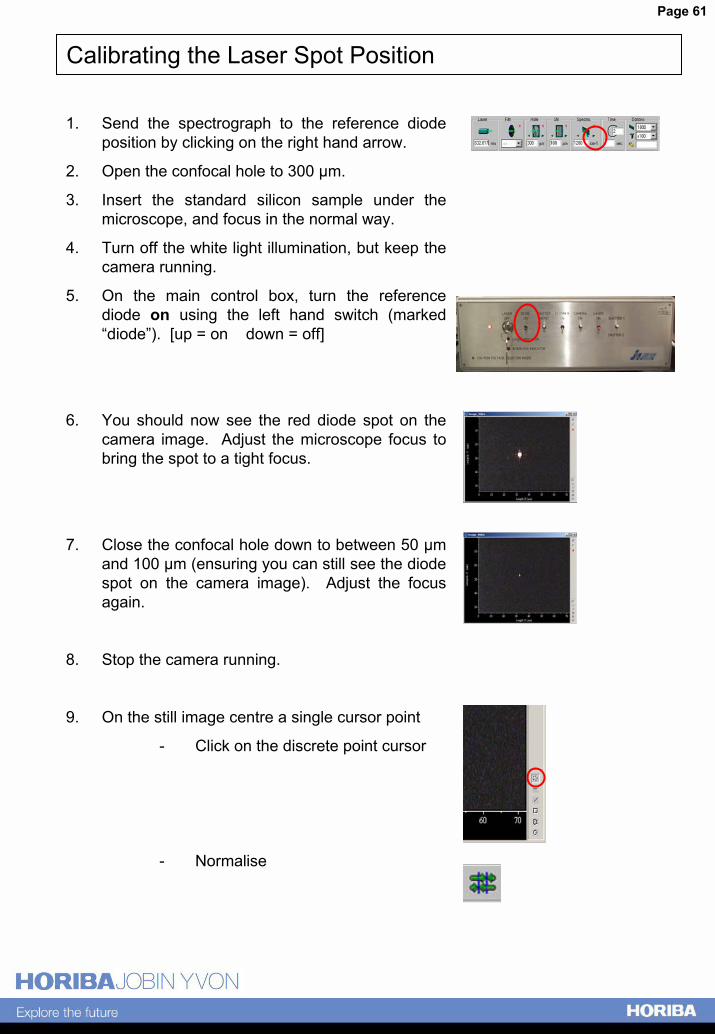
Calibrating the Laser Spot Position

1. Send the spectrograph to the reference diode position by clicking on the right hand arrow.

2. Open the confocal hole to 300 µm.

3. Insert the standard silicon sample under the microscope, and focus in the normal way.

4. Turn off the white light illumination, but keep the camera running.

5. On the main control box, turn the reference diode on using the left hand switch (marked �diode�). [up = on down = off]

6. You should now see the red diode spot on the camera image. Adjust the microscope focus to bring the spot to a tight focus.

7. Close the confocal hole down to between 50 µm and 100 µm (ensuring you can still see the diode spot on the camera image). Adjust the focus again.

8. Stop the camera running.

9. On the still image centre a single cursor point

- Click on the discrete point cursor

- Normalise

Page 62

Calibrating the Laser Spot Position - continued

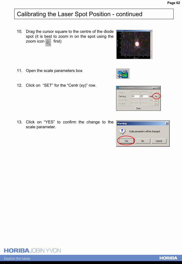
10. Drag the cursor square to the centre of the diode spot (it is best to zoom in on the spot using the zoom icon first)

11. Open the scale parameters box

12. Click on �SET� for the �Centr (xy)� row.

13. Click on �YES� to confirm the change to the scale parameter.

Page 63

Installing LabSpec Software for Data Analysis

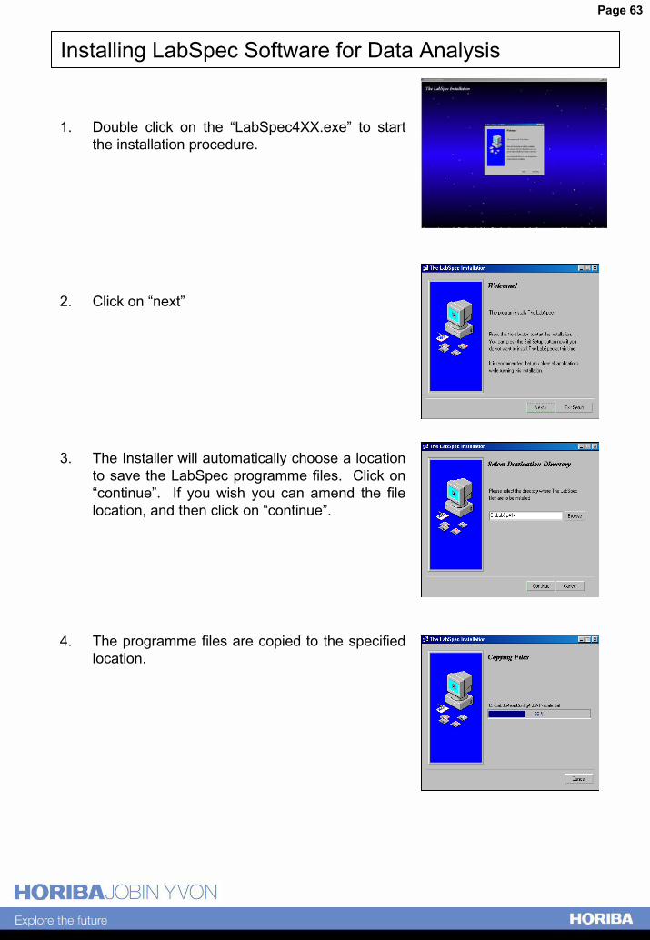
1. Double click on the �LabSpec4XX.exe� to start the installation procedure.

2. Click on �next�

3. The Installer will automatically choose a location to save the LabSpec programme files. Click on �continue�. If you wish you can amend the file location, and then click on �continue�.

4. The programme files are copied to the specified location.

Page 64

Installing LabSpec Software for Data Analysis - continued

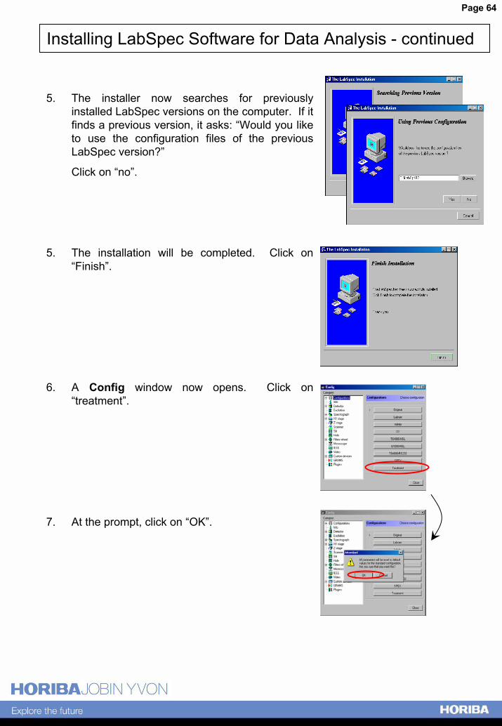
5. The installer now searches for previously installed LabSpec versions on the computer. If it finds a previous version, it asks: �Would you like to use the configuration files of the previous LabSpec version?�

Click on �no�.

5. The installation will be completed. Click on �Finish�.

6. A Config window now opens. Click on �treatment�.

7. At the prompt, click on �OK�.

Page 65

Installing LabSpec software for data treatment - continued

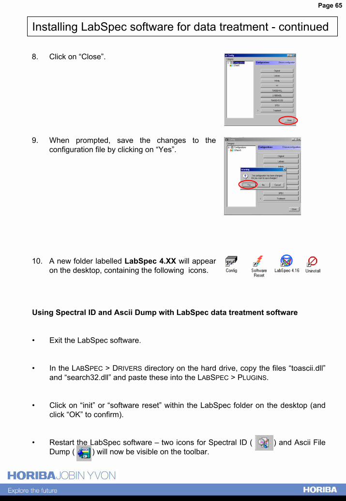
8. Click on �Close�.

9. When prompted, save the changes to the configuration file by clicking on �Yes�.

10. A new folder labelled LabSpec 4.XX will appear on the desktop, containing the following icons.

Using Spectral ID and Ascii Dump with LabSpec data treatment software

� Exit the LabSpec software.

� In the LABSPEC > DRIVERS directory on the hard drive, copy the files �toascii.dll�and �search32.dll� and paste these into the LABSPEC > PLUGINS.

� Click on �init� or �software reset� within the LabSpec folder on the desktop (and click �OK� to confirm).

� Restart the LabSpec software � two icons for Spectral ID ( ) and Ascii File Dump ( ) will now be visible on the toolbar.

Page 66

Section 6Contact Details

Page 67

Contact Details for Horiba Jobin Yvon

For further information in the UK please contact:

RAMAN SERVICE DEPARTMENT

For all enquiries concerning software, hardware, maintenance and service issues, including lasers, heating/cooling stages, and other accessories.

RAMAN SALES OFFICE

For all enquiries about software and applications, upgrades, new accessories and new instruments.

HORIBA Jobin Yvon Ltd.,

2, Dalston Gardens,

Stanmore,

Middlesex,

HA7 1BQ

Tel: 020 8204 8142

Fax: 020 8204 6142

http://www.jobinyvon.co.uk

http://www.jobinyvon.co.uk

Documents

LabRAM User Guide - Trinity College, Dublin · Simple 14 Multiwindow 14 ... The instrument can be considered in four parts: 1. Lasers Œthe HeNe ... functions, see next page. MICROSCOPE