LabVIEW Applications for Optical Amplifier Automated ... · LabVIEW Applications for Optical Amplifier Automated Measurements, Fiber-Optic Remote Test and Fiber Sensor Systems 203

10

LabVIEW Applications for Optical Amplifier Automated Measurements, Fiber-Optic Remote

Test and Fiber Sensor Systems

S. W. Harun, S. D. Emami, H. Arof, P. Hajireza and H. Ahmad University of Malaya

Malaysia

1. Introduction

For the past 20 years, intensive researches in the fields of optoelectronics and fiber optic communications have resulted in the invention of new devices that revolutionized our life. The optoelectronics devices such as compact disc players, laser printers, bar code scanners, and laser pointers are some of the examples [1]. In fiber optic communications, revolution in the telecommunications system has been initiated by the introduction of higher bandwidth, more reliable telecommunication links with lower bandwidth cost [2]. Recently, fiber optic sensor technology has gained interest from the research community. Optical fiber sensors offer a number of advantages over conventional electrical sensing technologies, which make them attractive for a wide range of application areas. These advantages include intrinsic safety in chemically hostile or explosive environments, low susceptibility to electromagnetic interference, electrically passive operation and high sensitivity, compatible with composites, light weight and geometrical versatility [3]. Improvement in fiber optic technology creates a necessity for a virtual instrumentation system. A virtual instrumentation system is software used for developing a computerized test system, a measurement system, a calibration system, a control system for an external measurement hardware device and a display system for test or measurement data [4]. The best virtual instrumentation system that has been developed so far is LabVIEW. LabVIEW is an application development program that was developed by National Instruments in 1986 to integrate science and engineering tasks by interfacing computers with instruments for collecting, storing, analyzing, and transmitting data while, at the same time, providing an effective user interface. Different from other development software such as C/C++, FORTRAN, Basic, etc., LabVIEW utilizes its own integrated programming language known as the Graphical Programming Language, which uses graphics as code sequences in the application being developed, making the software development process significantly easier [5]. LabVIEW is powerful programming software that can interface with over 7,000 instruments to provide data acquisition, industrial measurement, automated testing, and instrument control. Integrated through LabVIEW, instruments such as sensors, optical time domain reflectometer (OTDR), oscilloscopes, optical spectrum analyzer (OSA) and RF generators can work alongside the GPIB hardware application software that makes fiber optic communication system research activities significantly easier [6].

www.intechopen.com

Modelling, Programming and Simulations Using LabVIEW™ Software

202

In this chapter, applications of LabVIEW in automatic test measurement of fiber optic system are demonstrated. In the first section, the LabVIEW applications in fiber optic system and the basics of instrument connectivity are presented. Then, the aspects of hardware communication to external instruments through GPIB and serial interfaces are analyzed. Next, self-calibrating automated characterization system for depressed cladding applications is demonstrated utilizing the LabVIEW’s GPIB interface. The automation system consists of a tunable laser source (TLS), optical spectrum analyzer (OSA), attenuator, laser diode controller, and a personal computer all networked using GPIB cables. Results of the manual and automatic measurements and the analysis of the measurement trace obtained from the optical time domain reflectometer (OTDR) are shown. Subsequently, the communication methods between the OTDR device and personal computer along with the details of the automation program developed using LabVIEW are presented. In the end, two applications of LabVIEW in fiber optic sensor system are discussed.

2. LabVIEW for fiber optic applications

Fiber optic systems have become in high demand for use in telecommunication and sensor systems. The optical systems, whether transmitting data across continents or providing real time measurement consist of dozens of components. These components are made from many different types of exotic materials and the manufacturing technologies are so new. Traditional labor intensive techniques cannot keep up with market demands, which require a cheaper solution. This section explains the automatic test measurement, fiber sensor and remote testing, which can be used to solve many problems in fiber optic system.

2.1 Self-calibration automated measurement Automatic test measurement is a vital part of the telecommunication and fiber optic communication test scene today. Automatic test measurement enables self-calibrating test to be done very swiftly and accurately. The amount of time consumed in implementing a fiber optic sensor system forms the bulk of the development cost and thus it is necessary to reduce the troubleshooting time to the shortest possible. This can be achieved with the use of automatic test measurement techniques [6]. There are a variety of different approaches that can be used for automatic test measurement systems. Each type has its own advantages and disadvantages, and can be used to great effect in the right circumstances. Automatic test equipment and automatic test software are the two main types of test measurement systems. Equipments such as automatic optical inspection (AOI), automated X-Ray inspection (AXI) and In-Circuit Test (ICT) are common forms of automatic test equipment which are used today in optical and electrical science [4]. One the best solution in automatic test equipment is a board or unit that can be tested using a stack of remotely controlled test equipment. The most popular method of controlling the test equipment is the General Purpose Interface Bus (GPIB). There may also be an interface adapter necessary to control and interface with the item under test. While the GPIB is relatively slow and has been in existence for over 30 years it is still widely used as it provides a very flexible tool of test. This type of systems use test instruments on a board that can be slotted into a standard slot thus saving both space and cost when compared to the stand-alone. Laboratory test equipment can often be used as most items of lab test equipment have a GPIB port. The main drawback of GPIB is its speed and the cost of writing the programmes although packages like LabVIEW can be used to aid programme generation and execution in the test environment [5].

www.intechopen.com

LabVIEW Applications for Optical Amplifier Automated Measurements, Fiber-Optic Remote Test and Fiber Sensor Systems

203

2.2 Fiber optic sensor Fiber optic sensor is a device in which variations in the transmitted power or the rate of transmission of light in optical fiber are the means of measurement or control. The information could also be derived in terms of intensity, phase, frequency, polarization, spectral content, or other quantities. Physical parameters such as strain, temperature, pressure, velocity, and acceleration can be measured by fiber optic sensor. Immunity to electromagnetic interference (EMI) and radio frequency interference (RFI), elimination of conductive paths in high-voltage environments, inherent safety and suitability for extreme vibration and explosive environments, tolerant of high temperatures (>1450 C) and corrosive environments, light weight, and high sensitivity are the main advantages of fiber optic sensor over normal sensor [7]. Depending on the usage, fiber optic sensors can be divided into Extrinsic (or Hybrid) and Intrinsic (or All-Fiber) types. Figure 1 shows an extrinsic sensor which consists of an optical fiber that transmits modulated light from a conventional sensor. A major feature of extrinsic sensors, which makes them so useful in such a large number of applications, is their ability to reach places which are otherwise inaccessible. In an extrinsic sensor, sensing takes place in a region outside of the fiber [8]. An intrinsic sensor relies on the properties of the optical fiber itself to convert signals from the environmental into a modulation of the light beam passing through it. Intrinsic sensors can modulate the intensity, phase, polarization, wavelength or transit time of light. Sensors which modulate light intensity tend to use mainly multimode fibers, but only single mode cables are used to modulate other light parameters. A particularly useful feature of intrinsic fiber optic sensors is that they can, if required, provide distributed sensing over distances of up to 1 meter [7].

Fig. 1. Extrinsic sensor

Fig. 2. Intrinsic sensor

Input Fiber Output Fiber

Light Modulator

Environment Signal

Environment Signal

Fiber Optic

www.intechopen.com


204

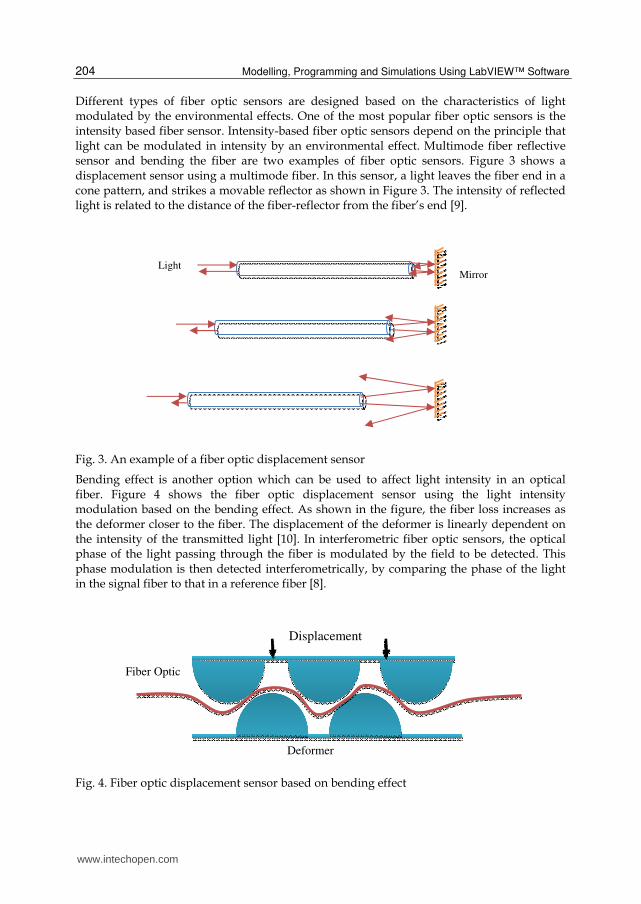
Different types of fiber optic sensors are designed based on the characteristics of light modulated by the environmental effects. One of the most popular fiber optic sensors is the intensity based fiber sensor. Intensity-based fiber optic sensors depend on the principle that light can be modulated in intensity by an environmental effect. Multimode fiber reflective sensor and bending the fiber are two examples of fiber optic sensors. Figure 3 shows a displacement sensor using a multimode fiber. In this sensor, a light leaves the fiber end in a cone pattern, and strikes a movable reflector as shown in Figure 3. The intensity of reflected light is related to the distance of the fiber-reflector from the fiber’s end [9].

Fig. 3. An example of a fiber optic displacement sensor

Bending effect is another option which can be used to affect light intensity in an optical fiber. Figure 4 shows the fiber optic displacement sensor using the light intensity modulation based on the bending effect. As shown in the figure, the fiber loss increases as the deformer closer to the fiber. The displacement of the deformer is linearly dependent on the intensity of the transmitted light [10]. In interferometric fiber optic sensors, the optical phase of the light passing through the fiber is modulated by the field to be detected. This phase modulation is then detected interferometrically, by comparing the phase of the light in the signal fiber to that in a reference fiber [8].

Fig. 4. Fiber optic displacement sensor based on bending effect

Light Mirror

Displacement

Fiber Optic

Deformer

www.intechopen.com


205

2.3 Remote fiber test system A Remote Fiber Test System (RFTS) is used mainly for error detection in optical networks that may arise due to mechanical faults or quality losses in the optical fibers and connectors that form the optical communication network [11]. Optical Time Domain Reflectometer (OTDR) is the main device for measurement and software control of the measurement process in RFTS. Figure 5 shows a simple RFTS measurement system. The control unit is a personal computer which is used for pre and post-measurement management. The OTDR functions as a measurement unit and the optical power splitter divides an input power equally into output ports. The optical power splitter can be replaced by an optical switch [12].

Fig. 5. RFTS measurement system.

The measurement process begins as the OTDR injects a short light pulse into the optical power splitter. In the splitter, the input power is divided into several output ports with power ratio specified by the splitter type. As the light pulse travels along the test fiber, a fraction of light is reflected back to the optical power splitter due to Rayleigh scattering and Fresnel reflection. All the scattered signals from the test fiber form a complex measurement trace as they reach the OTDR. Finally, the OTDR trace is saved in the computer memory and the analysis of the measurement result begins. In the standard RFTS, the error detection system is based on the measurement of the total loss in the optical link. Another approach that can be used is by comparing the reference and test measurement results. The reference measurement is collected just after the installation of the optical communication system [4]. As the test measurement is performed, the resulting test OTDR trace is compared with the reference trace. If the difference between the optical power level of the reference and the test measurement at certain measurement point exceeds the predefined threshold, the RFTS reports an error and stops the measurement. The time for the measurement to repeat is controlled by the user. The whole measurement process is software controlled and managed by LabVIEW [13].

3. Instrument communication methods

There are different types of communication methods available for controlling laboratory instruments as well as optical components. These methods are serial, parallel, GPIB, VXI,

www.intechopen.com


206

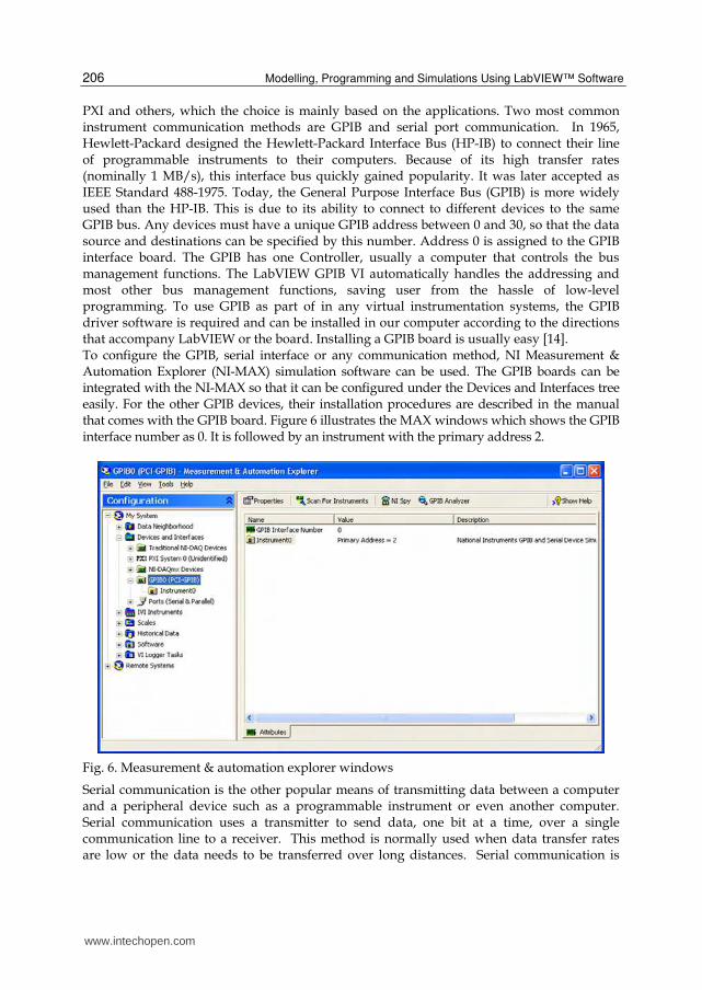
PXI and others, which the choice is mainly based on the applications. Two most common instrument communication methods are GPIB and serial port communication. In 1965, Hewlett-Packard designed the Hewlett-Packard Interface Bus (HP-IB) to connect their line of programmable instruments to their computers. Because of its high transfer rates (nominally 1 MB/s), this interface bus quickly gained popularity. It was later accepted as IEEE Standard 488-1975. Today, the General Purpose Interface Bus (GPIB) is more widely used than the HP-IB. This is due to its ability to connect to different devices to the same GPIB bus. Any devices must have a unique GPIB address between 0 and 30, so that the data source and destinations can be specified by this number. Address 0 is assigned to the GPIB interface board. The GPIB has one Controller, usually a computer that controls the bus management functions. The LabVIEW GPIB VI automatically handles the addressing and most other bus management functions, saving user from the hassle of low-level programming. To use GPIB as part of in any virtual instrumentation systems, the GPIB driver software is required and can be installed in our computer according to the directions that accompany LabVIEW or the board. Installing a GPIB board is usually easy [14]. To configure the GPIB, serial interface or any communication method, NI Measurement & Automation Explorer (NI-MAX) simulation software can be used. The GPIB boards can be integrated with the NI-MAX so that it can be configured under the Devices and Interfaces tree easily. For the other GPIB devices, their installation procedures are described in the manual that comes with the GPIB board. Figure 6 illustrates the MAX windows which shows the GPIB interface number as 0. It is followed by an instrument with the primary address 2.

Fig. 6. Measurement & automation explorer windows

Serial communication is the other popular means of transmitting data between a computer and a peripheral device such as a programmable instrument or even another computer. Serial communication uses a transmitter to send data, one bit at a time, over a single communication line to a receiver. This method is normally used when data transfer rates are low or the data needs to be transferred over long distances. Serial communication is

www.intechopen.com


207

popular because most industrial computers have at least one serial port available. However, for laptops and smaller desktops that do not have a built-in serial port, an inexpensive USB-to-RS-232 adaptor can also be used. Serial communication requires that you specify four parameters: the baud rate of the transmission, the number of data bits encoding a character, the sense of the optional parity bit, and the number of stop bits. The requirements for port setting features are shown in the Ports (serial and parallel) menu in Figure 7. For the port binding, it is used for specifying the port to be used for the serial/parallel device. An alternative port can be selected to link to the ASRL resource, this setting does not change the logical port number (COMx) of the physical serial port, it only changes which COM port this VISA resource is binding to. After that, click the “Validate” button to test whether NI-VISA can access the resource with the specified configuration. The result shown on Figure 8 should pop up.

Fig. 7. Serial port setting

Fig. 8. Validation of NI-MAX

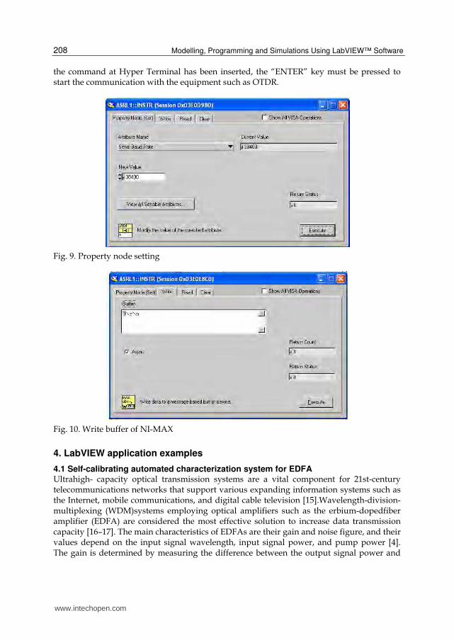
When a VISA session to “ASRL1::INSTR” is successfully opened, communication with the device can be started by going to the Property Node (Set) and modifying the value of the specified attribute as shown in Figure 9. The values for serial baud rate, serial data bits, serial stop bits, serial flow control and others are set to the same values as those chosen during Port Setting. Then click the execute button. Next, as shown in Figure 10, click the “Write” tab and fill up the blank box under the “Buffer” with a proper command ending with “\r\n” to initiate the communication with the serial device. The function of “\r\n” is just like the “ENTER” button on a personal computer keypad. Without “\r\n”, the command is incomplete, and hence, NI-MAX cannot recognize it. This is the same as when

www.intechopen.com


208

the command at Hyper Terminal has been inserted, the “ENTER” key must be pressed to start the communication with the equipment such as OTDR.

Fig. 9. Property node setting

Fig. 10. Write buffer of NI-MAX

4. LabVIEW application examples

4.1 Self-calibrating automated characterization system for EDFA Ultrahigh- capacity optical transmission systems are a vital component for 21st-century telecommunications networks that support various expanding information systems such as the Internet, mobile communications, and digital cable television [15].Wavelength-division-multiplexing (WDM)systems employing optical amplifiers such as the erbium-dopedfiber amplifier (EDFA) are considered the most effective solution to increase data transmission capacity [16–17]. The main characteristics of EDFAs are their gain and noise figure, and their values depend on the input signal wavelength, input signal power, and pump power [4]. The gain is determined by measuring the difference between the output signal power and

www.intechopen.com


209

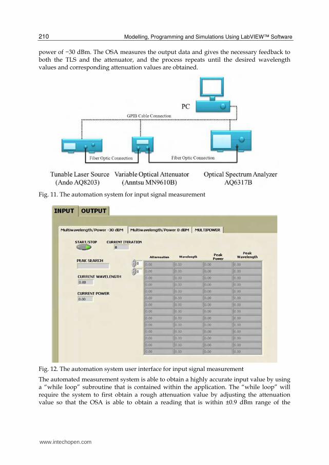
the input signal power, whereas the noise figure is calculated from the gain, amplified spontaneous emission (ASE), and resolution of the optical spectrum analyzer (OSA). The accurate ASE level is measured using the interpolation technique, and thus, even a slight error in the initial measurement of the input power level will cause a cascading effect that will render the final ASE measurement invalid. In addition, the accuracy of the gain value is also dependent on the accuracy of the input measurement [5]. This makes the current manual measurement techniques not suitable for gain value measurement as even the slightest deviation in the initial input measurement will result in inaccurate gain values. As such, using manual measurement techniques for EDFA experiments could lead to inaccurate results and long experiment times. EDFAs are typically characterized using OSAs, tunable laser sources (TLSs), optical attenuators, laser diode controllers, and optical power meters. From experience, EDFA research with manual control of these instruments will lead to delays and inaccuracies in research due to the large number of values that have to be taken and recalibrated for each parameter. To cope with this problem, a self-calibrating automated measurement system for EDFAs has been developed based on the LabVIEW program and GPIB hardware. The basic architecture of a standard EDFA is depicted in Figure 11. The setup consists of a piece of EDF, a wavelength division multiplexing (WDM) coupler, a pump laser and two isolators. In this work, a depressed cladding EDF (DC-EDF) with Erbium ion concentration of approximately 500 ppm is used as gain medium for amplification in S-band region. The EDF is pumped by a 980 nm laser diode to generate population inversion for amplification. A WDM coupler is used to combine the pump light with the input signal. Optical isolators are used to ensure unidirectional operation of the optical amplifier [15].

Fig. 11. Configuration of the EDFA

The automation system consists of a TLS, OSA, attenuator, laser diode controller, and a personal computer. All these instruments are networked using GPIB cables and are individually designated as Talkers, Listeners, and/or Controllers. By having these functions, all the involved instruments can automatically be controlled through a single computer for the input signal measurement; the experiment is setup as shown in Figure. 11, using only the TLS, attenuator, and OSA. Figure 12 shows the user interface of the automation system. The program has two main menus, i.e., the “input” menu and the “output” menu. Under the “input” menu, there are three submenus, i.e., “Multiwavelength/Power −30 dBm,” “Multiwavelength/Power 0 dBm,” and “Multipower.” The “Multiwavelength/Power −30 dBm” submenu measures data by fixing the input power at −30 dBm and varying the input signal wavelengths. This submenu automatically changes the TLS wavelength values and determines the most accurate corresponding attenuation value to obtain a constant input

www.intechopen.com


210

power of −30 dBm. The OSA measures the output data and gives the necessary feedback to both the TLS and the attenuator, and the process repeats until the desired wavelength values and corresponding attenuation values are obtained.

Fig. 11. The automation system for input signal measurement

Fig. 12. The automation system user interface for input signal measurement

The automated measurement system is able to obtain a highly accurate input value by using a “while loop” subroutine that is contained within the application. The “while loop” will require the system to first obtain a rough attenuation value by adjusting the attenuation value so that the OSA is able to obtain a reading that is within ±0.9 dBm range of the

www.intechopen.com


211

required −30dBm value, as per the requirement of the multiwavelength menus or as per the required power as determined by the user in the multipower menu. Once the rough attenuation of the value has been determined, the system will then adjust the attenuation value based on the OSA readings to obtain the exact attenuation value required for the subsequent experiment. The “while” loop is illustrated in Figure 13. The submenu “Multiwavelength/Power 0 dBm” gathers data at a constant 0 dBm input power at different wavelengths. With regard to wavelength, the software is programmed for the S-band wavelength region from 1480 to 1530 nm. The “Multipower” submenu obtains the input power for a constant center wavelength, but at different input powers, which has been programmed from −40 to 5 dBm. All submenu functions are automatic, and the software records all required data on either diskette or hard disk.

Fig. 13. “while loop” subroutine

TLS ON

ATTN 0dB

OSA Obtain Input Power Value

Attenuation =input signal Value- 40 dBm

OSA Attenuation Rough calibrations

39.1>M>40.9 No

OSA Attenuation Fine

Store Attn Value

Yes

ｨ=40 ｿBﾈ

www.intechopen.com


212

For EDFA gain and noise figure measurements, the apparatus is set up as shown in Figure 14. The EDFA is placed between TLS and OSA, with the laser diode controller pumping the EDF (the pump power value must first be determined). The EDFA software “Output” menu is designed to automate this setup, as shown in Figure 15. Under the “Output” menu, there are two submenus, i.e., “Multiwavelength” and “Multipower.” The “Multiwavelength” submenu obtains such output data as the gain, noise figure, ASE, peak power, and peak wavelength, and the obtained data are compared with the input data taken from the “Multiwavelength −30 dBm” or “Multiwavelength 0 dBm” submenu first. This comparison of input and output data is done to obtain the gain and noise figure values using interpolation techniques.

Fig. 14. The automation system for output gain and noise figure measurements

Fig. 15. The automation system user interface for gain and noise figure measurement

www.intechopen.com


213

The “Multipower” submenu obtains output data at a center wavelength of 1500 nm but at different input powers. As with the “Multiwavelength” submenu, all data obtained from the “output” menu “Multipower” submenu are compared with data obtained from the “input” menu “Multipower” submenu to obtain values such as gain, noise figures, etc. All the “output” submenus plot graphs after one experiment cycle is complete, as shown in Figure 16, saving time for data analysis. In addition, the obtained data can also be stored in Word, Powerpoint, Excel, and other formats for further analysis. Figure 17 shows the flowchart for the automation system. The basic software design methodology possesses the required characteristics of being time efficient and the ability to accurately and consistently gather data while simultaneously reducing the uncertainty value, as these characteristics are very important in ensuring that the software can be utilized to gather data. The EDFA automation system is tested based on the aforementioned characteristics. The software is proven to reduce the EDFA testing time by more than 80%, as compared to manual EDFA testing methods.

Fig. 16. S-band EDFA software “Output” menu

Accuracy is also increased, as at times, the experimentalist can make mistakes in acquiring and analyzing the data. By using the automation software, the human error factor can be eliminated, thus providing a higher degree of accuracy. The uncertainty value is also determined to be approximately ±0.012 dB, as compared to manual testing methods, as shown in Figures 18 and 19. However, each new experiment cycle will require the recalibration of equipment. This is due to changing environmental conditions such as temperature and experimental setup alignment, which have a significant effect on the measurements taken by the equipment. In addition, the optical connectors cannot be removed during the experiment cycle, and a recalibration must be performed by the automation software if the optical connectors are removed. For OSA calibration, standard lamps are frequently used to calibrate the OSA, whereas power measurements are made using a standard lamp and a power detector. In addition to increased accuracy and a reduction in the experiment time, the software also reduces the number of personnel needed for each experiment, thus allowing personnel to focus more on the interpretation of the acquired data. In addition, the software is designed to be user friendly and does not require specialist training to operate.

www.intechopen.com


214

Fig. 17. Flowchart for the automation system.

Fig. 18. Automate and manual EDFA’s gain versus input signal power

Start

Select

Menu

Select Sub

Menu

Input Output

Multiwavelengt

hwith -30dBm

Input Power

Multi Power Multiwaveleng

Multi Power

Start Automatic

Measurement

Data Display and

Save

Stop

Sﾀﾇﾀｾﾏ Sﾐｽ

ｨﾀﾉﾐ

ｨﾐﾇﾏﾄﾒｼﾑﾀﾇﾀﾉﾂﾏ

ﾃﾒﾄﾏﾃ 0ｿBﾈ

Iﾉﾋﾐﾏ Pﾊﾒﾀﾍ

www.intechopen.com


215

Fig. 19. Automate and manual EDFA’s gain versus input signal wavelength

4.2 Remote fiber test system using Optical Time Domain Reflectometer (OTDR) DWDM has increased fiber traffic capacity and thus it is important to proactively monitor

and maintain the fiber networks. Due to huge penalties specified in Service Level

Agreements (SLAs) and Quality of Service (QoS) commitments, carriers are keen to take

measures in maintaining their fiber network. Optical Time Domain Reflectometer is a well-

known optoelectronic instrument used for testing a fiber optic cable assembly in optical

network [18]. An OTDR emits a pulsed ray into the fiber under test and acquired reflected

ray. The strength of the return pulses is measured and integrated as a function of time, and

is plotted as a function of fiber length. The plot can be used to analyse the optical fiber and

detect the approximate location of the fault event that occurred. Different pulse widths in

OTDR will affect the distance resolution and dynamic range. A longer laser pulse width will

improve dynamic range and attenuation measurement resolution at the expense of distance

resolution. This is useful for getting the overall characterization of a link, but is weak when

trying to locate faults. A short pulse width will improve distance resolution of optical

events, but will also reduce measuring range and attenuation measurement resolution [19].

Theoretically, OTDR has good distance measuring accuracy since it is software based and

with its crystal clock possesses an inherent accuracy of better than 0.01%. Further calibration

process is not needed since the practical cable length measuring accuracy is typically limited

to about 1% [20].

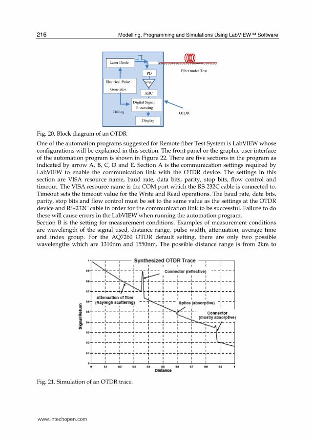
Figure 20 shows the block diagram of an OTDR where a laser diode is driven by an electrical

pulse generator that produces a train of short optical pulses. The backscattered optical

power from the fiber through a directional coupler is detected by photodiode (PD). The

detected waveform is amplified by an amplifier and converted to digital signal through the

analog to digital converter (ADC) and then processed by the digital signal processing (DSP)

unit. The timing of the DSP is synchronized with the source of the optical pulses so that

delay in the propagation of each scattered pulse can be precisely calculated. Figure 21 is a

typical commercial OTDR trace, showing among other things, the fiber attenuation. This

figure shows that different losses will have different shapes in the trace. Hence, the analysis

of the trace can be done to estimate the cause of a fault event [21].

www.intechopen.com


216

Fig. 20. Block diagram of an OTDR

One of the automation programs suggested for Remote fiber Test System is LabVIEW whose configurations will be explained in this section. The front panel or the graphic user interface of the automation program is shown in Figure 22. There are five sections in the program as indicated by arrow A, B, C, D and E. Section A is the communication settings required by LabVIEW to enable the communication link with the OTDR device. The settings in this section are VISA resource name, baud rate, data bits, parity, stop bits, flow control and timeout. The VISA resource name is the COM port which the RS-232C cable is connected to. Timeout sets the timeout value for the Write and Read operations. The baud rate, data bits, parity, stop bits and flow control must be set to the same value as the settings at the OTDR device and RS-232C cable in order for the communication link to be successful. Failure to do these will cause errors in the LabVIEW when running the automation program. Section B is the setting for measurement conditions. Examples of measurement conditions are wavelength of the signal used, distance range, pulse width, attenuation, average time and index group. For the AQ7260 OTDR default setting, there are only two possible wavelengths which are 1310nm and 1550nm. The possible distance range is from 2km to

Fig. 21. Simulation of an OTDR trace.

Laser Diode

Display

ADC

PD

Electrical Pulse

Generator

Digital Signal

Processing

OTDR Timing

Amp.

Fiber under Test

www.intechopen.com


217

Fig. 22. Front panel of the automation program

640km. The pulse width is from 0ns to 20us as provided by the manufacturer. The possible attenuation settings are from 0dB to 26.25dB according to the AQ7260 OTDR user manual. Finally, the group index with is varying from 1.00000 to 1.99999. Next is the measurement conditions output given in Section C. The blank space will display the output of the “fiber type with wavelength, distance range, pulse width, attenuation and resolution of the measurement”. The byte count1 value is set to more than the possible return count1 to prevent any loss of data. Users can enable or disable this function by clicking the “Save to USB” button. Finally, section E provides the measurement results. The measurement results in term of “event number, distance, splice loss, return loss, cumulative loss, dB/km, event type, and total span ORL” are shown in the blank area after the completed run of the program. For the event number, it will show “END” if the event is at end of the fiber, else it will show “1”, “2” and so on according to the number of the detected event. Some of the measurement results will be neglected if they are not detected by the OTDR measurement, and the only display values are for those detected by the OTDR. The whole program consists of 6 main stacked sequences and 20 sub stacked sequences. Figure 23 depicts the configuration for the distance range setting for the second main stacked sequence or the sub stacked sequence. VISA Write is used to write the data from write buffer to the device. The command for distance range is Rm\r\n, where “m” depends on the distance range chosen by the user. Figure 24 shows the configuration for pulse width programming. In the second sub stacked sequence, the command needed for the pulse width is PWm\r\n. The configuration for the programming of group index is shown in Figure 25. The command needed is IORm\r\n, in this case, the “m” is the range from 1.00000 to 1.99999 depending on the value needed for the user. The “concatenate strings” function will combine the two constants (IOR and \r\n) and the control (value of group index) in the arrangement from top to bottom to form IORm\r\n. Thereafter, the concatenate output string will pass to

C

A B D E

www.intechopen.com


218

Fig. 23. Programming for distance range

Fig. 24. Programming for pulse width

VISA Write to initialize the related operation. The next step is to initialize the OTDR device to start the measurement from the personal computer. The command needed to initialize the real time measurement is ST2\r\n. This command is sent to the VISA and the output is connected to the next sub stacked sequence. The duration needed for the OTDR measurement to be completed is approximately 15sec, so, a 20 second delay is applied to the next sub stacked sequence as shown in Figure 26 to ensure the measurement process is 100 percent complete. Then, to stop the measurement after 20 seconds, a stop measurement command is needed which is ST0\r\n, as shown in Figure 26. Without this stop command, the measurement will keep going without end.

VISA write

Concatenate strings

2nd Sub stacked sequence

2nd main stacked sequence Sub stacked sequence

Concatenate string

Number to decimal strings

Sequence local

www.intechopen.com


219

Fig. 25. Programming for group index

Fig. 26. Programming for stop measurement

For the automation program, the user has the option to choose whether they want to save a copy of the measurement trace and data or not. If the user does not wish to save the measurement trace, the program configuration at LabVIEW is as shown in Figure 27. The case structure is at the false condition (save function disable at the front panel). There is nothing to process or pass through during this sequence, hence, the program will continue to the next main sequence. If the user wishes to save a copy of the measurement results, the program configuration is shown in Figure 28. The case structure is at the true condition (save function enabled at the front panel). The configuration shown in Figure 28 is for the drive setting and file name to be saved for the measurement results. The command used is FDAmp\r\n (refer to Table 1), where “m” in this case is for drive setting and is equal to 5,

6th Sub stacked sequence

VISA write

Concatenate strings

VISA write

www.intechopen.com


220

which sets the drive used to save data to USB drive. While, “p” indicates any file name that the user wishes to save. The strings will be combined into a single output by the “concatenate strings” function and act as the input to the VISA Write. A delay is implemented to reduce the traffic to the OTDR to prevent the occurrence of a hang situation.

Fig. 27. Programming for false (save function disable)

Fig. 28. Programming for true (save enable) case, drive setting and file name to save

Figure 29 shows the configuration to set the file type of the measurement trace. Examples of the possible file types are BMP, SOR (Telcordia) and so on. The command used here is FF7\r\n, which will set the file type to be saved in the SOR format. This file format will assist the user when analyzing or modifying the measurement trace by using Yokogawa OTDR Viewer software. Again, a delay is applied to reduce the traffic to the OTDR to prevent hang up. Finally the “data save” command is used to save the data. Figure 30 shows that the command FST\r\n is sent to the input of the VISA Write. Then, the measurement trace or data will be completely saved into the device (pen drive or thumb drive) plugged into the USB port of the OTDR device. A delay of few seconds is needed for the measurement trace or data to be successfully saved into the pendrive or thumbdrive.

Case structure (for false case)

6th main stacked sequence

www.intechopen.com


221

Fig. 29. Programming for “file type save”

Fig. 30. Programming for data save.

The end of the program is as shown in Figure 31. This automation program ends with a

VISA Close. The VISA Close closes a device session or event object specified by the VISA

resource name. Finally, the simple error handling function indicates whether an error has

occurred. If an error occurs during the program execution, it will return a description of the

error and optionally displays it in a dialog box. In this section, the measurement data

obtained from the automation program are presented. These data will be used to compare

with the data obtained without using the automation program in the next section.

The results obtained from the automation program for 1310nm wavelength single mode

fiber at 100ns, 200ns and 500ns pulse width are printed on the screen and shown in Figures

32, 33 and 34. The data shown are the event number, distance, splice loss, return loss,

cumulative loss, dB/km, event type and the total return loss. The data are separated by

comma and is ignored if there is no such data for the certain event. The event number is in

accordance with the sequence of the events.

VISA write Wait (ms)

VISA write

www.intechopen.com


222

Fig. 31. Closes of the program

Fig. 32. 1310nm SMF at 100ns pulse width (automation program)



To verify the reliability of the automation program, a comparison between the results obtained from the automation program and the manually measured OTDR device is made. The data of Figures 35, 36 and 37 are obtained manually for 1310nm wavelength SMF at 100ns, 200ns and 500ns pulse width respectively. These results are compare with those obtained from the automation program. By comparing Figures 32, 33 and 34 with Figures 35, 36 and 37, it can be observed that the results are identical without any deviation. Hence,

VISA close

Simple error handler

www.intechopen.com


223

it is concluded that the automation program is very reliable and the results obtained from automation program are exactly the same as those obtained from the manually measured data from the OTDR device.

Fig. 35. 1310nm SMF at 100ns pulse width (manually measurement)



www.intechopen.com


224

4.3 Automated fiber optic multiphase dynamic fluid differentiation measurement Nowadays the main concern for many industries, especially those related to power production and more importantly the oil and gas industry is the discrimination of the immiscible phases of fluids in a flow system. The phase differentiation method is one of the effective, low-cost and highly accurate methods to discriminate phases in a flow system [22]. This ability to discern between the various phases of a flow system is important as this will ultimately affect the production outcome of the system. Oblique tips is one of the effective ways to achieve phase discrimination in fiber optic sensor. However, a proper automation and analysis software is necessary for the interpretation of the data from the optical probes [23], [24]. The LabVIEW software is a smart analysis program which is able to discriminate the individual phases of a multiphase system using Boolean logic and it presents the data in a real-time manner. Discrimination of the immiscible phases of fluids in a flow system using the phase differentiation measurement method is demonstrated by Kavintheran in 2007 [25]. The software was designed to monitor up to 8 individual sensor probes and it can also be configured to monitor two-phase or even three-phase flows. The automated measurement of the phase differentiation measurement system is demonstrated in Figure 38. The system consists of four optic sensor heads, four laser diodes, four optical circulators, an optical coupler and an OSA. The laser diodes work as signal sources which send signal through the circulator to the optic sensors. The sensor head assembly is designed such that the sensor probes are arranged 90 degrees apart at 0, 90, 270 and 360 respectively. The reflected signal from the optic sensor head goes back to the circulator and is redirected to combine with reflections from the other laser sources through the OSA. The OSA is connected via GPIB hardware to a computer equipped with the LabVIEW software and a phase discrimination program that uses Boolean logic to accurately determine the various phase fractions of the multiphase system in real-time.

Fig. 38. Sensor probe location in sensor head assembly

The system is designed so that the output for each probe that computes a reflectivity between 0.015 and 0.040 generates a digital “1” which indicate water, and a digital “0” for each probe that computes a reflectivity of less than 0.015 to indicate air. The system

www.intechopen.com


225

incorporates a Boolean logic function that allows the phase level measurement to be determined accurately and also without any overlay in data. Figure 39 shows the flowchart for the operation of the program, while Figure 40 below shows the Boolean logic circuit. To detect three possible indications of the phase level, the Boolean logic function is designed to accommodate up to eight sensor probes. The three possible results are one-quarter water three-quarters air, three-quarters water one-quarter air and full water. Visual representation of the phase level is the result of the outputs of the logic circuit which is connected to the indicators. Each sensor probe is connected to an OR gate. In order to allow the logic functions to operate with only one input, OR gates are used. The OR gate allows the deployment of either four sensor probes or eight sensor probes. The program will refresh the phase fraction levels every 1 second, which is the scan time of the OSA [25].

Fig. 39. Phase discrimination program flowchart

Fig. 40. Boolean logic function for phase discrimination

Read Probe 1

0.015 <

R< 0.040

Indicate=1 Iﾉｿﾄｾｼﾏﾀ=0

Yes

No

Read Probe 1

0.015 <

R< 0.040


Yes No

Read Probe 1

0.015 <

R< 0.040


Yes No

Read Probe 1

0.015 <

R< 0.040


Yes No

Sﾏｼﾍﾏ

Iﾉｿﾄｾｼﾏﾀ Pﾃｼﾎﾀｧﾀﾑﾀﾇ

Bﾊﾊﾇﾀｼﾉｧﾊﾂﾄｾ Fﾐﾉｾﾏﾄﾊﾉ

www.intechopen.com


226

The reflectivity of the probes as a function of time when the water level in the flow system is at one-quarter is shown in Figure 41. As depicted, the reflectivity of probe 3 in water is shown to be 0.032 by the software, while the reflectivity’s of probes 1, 2 and 4 is shown to be 0.002. To determine the phase level of the system, the Boolean logic function is done automatically and immediately. When digital “1” signal is generated by probe 3, it immediately passes through the respective logic gates to determine the phase level. Once this has been done, the system will represent the phase level using a diagram as shown in Figure 42. When the flow system is half-full, the reflectivity of probes 2, 3 and 4 is 0.0316, while the reflectivity of probe 1 remains at 0.002. Figure 43 shows the reflectivity of the four probes against time.

Fig. 41. Reflected power (dBm) of sensor probe vs. time for one-quarter full flow system

Fig. 42. LabVIEW phase level representation for one-quarter full flow system

Similarly, the Boolean logic gate function will determine the phase level of the system as shown in Figure 44. When all four probes detect water, the reflectivity of all four probes is 0.002, as shown in Figure 45. The Boolean logic system will then determine the phase level of the system to be fully water, and will indicate the condition of the system as shown in Figure 46.

www.intechopen.com


227

Fig. 43. Sensor probe reflectivity of vs. time for half-full flow system

Fig. 44. LabVIEW phase level representation for half-quarter full flow system.

Fig. 45. Sensor probe reflectivity of vs. time for full flow system

www.intechopen.com


228

Fig. 46. LabVIEW phase level representation for full flow system

4.4 Polarimetric fiber-optic pressure sensor Due to the possibility of it being used to distribute high sensitivity sensors and of it being

configurable in many different shapes, the polarization–based FOS is widely used. Recently

different types of polarimetric sensors have been investigated for the measurement of

various physical parameters such as: pressure, strain, stress and temperature. Polarimetric

fiber optical sensors are sensitive to the variations in the polarization state of light

transmitted by a single mode optical fiber. The state of polarization may vary according to

physical factors such as stress, pressure, temperature, etc [26]. So far, the polarimetric fiber

sensors demonstrated in the literature are based on interferometric schemes. In

interferometric schemes high-birefringent (HB) polarization maintaining (PM) fibers are

used. The proposed fibers have strong asymmetries so the quasi-degeneracy of the two

orthogonally polarized modes can be avoided and thus forcing a single polarization mode

under normal operations.

A low-cost distributed deformation sensor based on the change of polarization in a standard

single-mode fiber of which data is obtained by the help of LabVIEW has been successfully

developed by G. C. Contantin [27]. The schematics of the sensor is shown in Figure 47 which

consists of a laser source, a mechanical polarization controller, a fiber polarizer and an

optical receiver that is connected to a PC via a digital acquisition card (DAQ). The Power

source consists of a laser diode and the biasing circuit. The laser source which is used is a

telecommunications laser diode mounted inside a butterfly package. To acquire the diode

temperature and monitor its temporal evolution, a laser diode is connected to a PC via a

digital acquisition card. The light emitted by the laser source feeds the pressure transducer

via the mechanical polarization controller that is used to align the incident polarization

orthogonal to the transmission axis of the polarizer in the absence of the applied pressure

stimulus. In this situation, the receiver reads a “0” voltage in the absence of any

perturbations. It is also possible to align the light polarization in order to maximize the

receiver reading in the idle state. As shown in Figure 47, the pressure sensor is made of a

fiber sandwiched between two plexiglass plates [27]. Under pressure, the polarization state

of the single-mode fiber changes and the value of the power transmitted from the fiber

polarizer is affected. Therefore, if an optical power of zero is registered in the absence of

www.intechopen.com


229

perturbation, once pressure is applied to the transducer an optical power other than zero is

obtained at the receiver [27].

Fig. 47. Distributed deformation sensor schematic

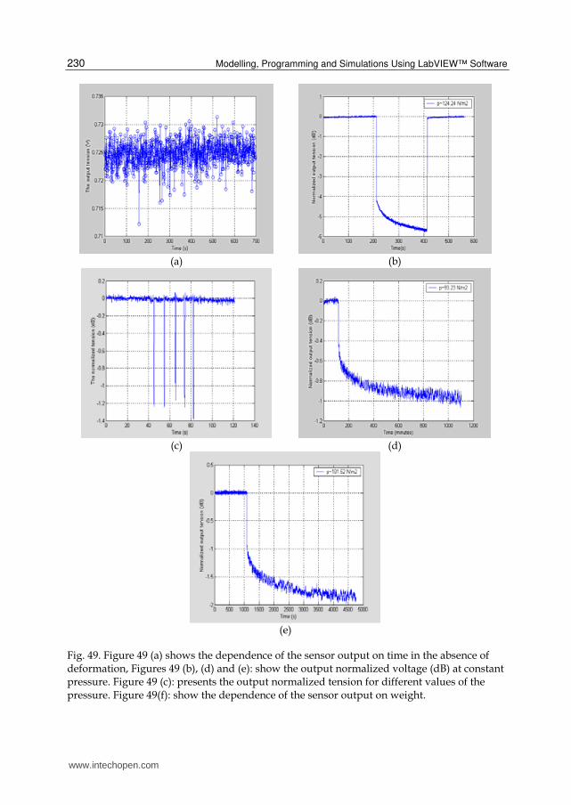
Figure 48 shows the data acquisition program which has been developed with LabVIEW

software. The main results obtained using the polarimetric fiber-optic pressure sensor is

shown in Figure 49. In these figures, the dependency of the sensor output on time is shown.

Figure 49(a) shows the output voltage (V) versus time in the absence of deformation. Figure

49 (c) presents the output normalized tension for different values of the pressure. The

Fig. 48. Data acquisition program

Receiver

Mechanical Polarization Controller

In-line Polarizer

Laser Diode

Optical Coiled Fiber

Pressure

Plexiglass

www.intechopen.com


230

(a)

(b)

(c)

(d)

(e)

Fig. 49. Figure 49 (a) shows the dependence of the sensor output on time in the absence of deformation, Figures 49 (b), (d) and (e): show the output normalized voltage (dB) at constant pressure. Figure 49 (c): presents the output normalized tension for different values of the pressure. Figure 49(f): show the dependence of the sensor output on weight.

www.intechopen.com


231

output normalized voltage (dB) at constant pressure is shown in Figures. 5 (b), (d) and (e).

The normalized value is calculated by [27]

(0)

out infnorm

out inf

V VV

V V

−= −

Where Vnorm represents the output normalized voltage, Vout is the value of the acquired

voltage, Vinf =− 0.5V is the lower limit of the output voltage and out (0) V is the output

voltage in the absence of deformation.

4.5 Fiber Bragg Grating (FBG) sensor interrogation system Recently in the field of architecture and civil, infrastructures such as long-span bridges,

high-rise buildings, large dams, nuclear power stations, off shore platforms and others,

there is a great demand for high performance sensors for structural health monitoring

(SHM) systems to guarantee the efficiency/safety of the structures. Optical Fiber sensors

such as the Fiber Bragg Grating (FBG) shows distinguishing advantages: immunity to

electromagnetic interference and power fluctuation along the optical path and high

precision. An FBG is a type of Bragg reflector constructed in a short part of optical fiber that

reflects particular wavelengths of light and transmits all others. A key research area in FBG

sensors is FBG fabrication, FBG demodulation and FBG encapsulation. In order to push

forward the applications of the FBG sensors, reliability and accuracy of the FBG sensors

must be ascertained. To achieve accuracy in the interrogation system, there is a great need in

a monitoring program that could process the data and display the data collected for each

sensor in graphical forms [28]. The optics, hardware and software architecture of such

system was developed in year 2005 by Toh Yue Khing [29]. In this FBG fabrication system,

digital filtering, peak detection and the ability to lock onto the reference wavelength are

implemented by the LabVIEW program. In this research work, FBG is fabricated by using

photosensitized optical fibers where the fiber reflective index is imprinted within the fiber

core. The FBG sensor is fiber with different reflective indices which are connected in series

to increase the number of sensors in a single fiber optic channel. Under tension or

compression, changes in the reflective indices in the fiber will cause a shift in the reflected

wavelength. By measuring the change in wavelength of the reflected light, the FBG

interrogation system will be able to measure temperature, pressure or strain changes,

depending on the types of material embedded in the FBG [29].

Figure 50 shows the interrogation System designed for the FBG fabrication system. As

shown, a PCI-7831R FPGA Module, Fiber Fabry Perot Tunable Filter (FFP-TF), 8

photodiodes, 8 Pre-amps and an 8-Channel Fiber Optic Configuration are used in the

system. Fiber Fabry Perot is a tunable filter which allows a narrow band of wavelength to

pass through the fiber and filters the broad band laser. The Fabry Perot Tunable Filter is

very sensitive to voltage change and serious noise disturbance produced by the electronic

circuitry can also affect the accuracy of the result. Therefore, a high precision and low noise

DAC voltage set is required. The PCI-7831R is a national instrument multifunction board

featuring a user-programmable FPGA chip for onboard processing and flexible I/O

operation. All analog and digital functionality is configured using the NI LabVIEW

graphical block diagrams and the LabVIEW FPGA Module. When the PCI-7831R receives

www.intechopen.com


232

instructions from LabVIEW to perform a scan, it will instruct the DAC to send out a whole

range of voltage from 0 to 10V. At each change of DAC output, the FPGA will read from the

8 ADCs simultaneously and store the raw data onto the onboard memory. Once completed,

data in the memory will be digitally filtered using the LabVIEW program.

The main software filters the noise from the data that is caused by both optical and electrical

disturbance. Since the tunable filter is sensitive to temperature, the characteristic of the filter

tends to drift over time. This drift will cause an error in the measurement. Thus, the

software will automatically lock onto a reference FBG to obtain an accurate reading. The

software front panel consists of two tabs. Figure 51 shows the sensor view tab. As shown in

Figure 50, every peak in the FBG sensors is represented by the strain, pressure or

temperature gauge. Any shift in wavelength of the FBG sensors will cause the measurement

gauge to respond.

Fig. 50. Interrogation System design using FBGs

The scope view tab of the waveform acquired from the interrogation system developed for

one of the channels is shown in Figure 52. These tabs consist of two scope displays. The top

display shows the filtered data, while the bottom display shows the raw data from the

Interrogation System. The first peak is the reference FBG and the rest of the 10 peaks are

from 10 different types of FBG sensors. The shifting of peak 9 is caused by a change in

pressure applied to the FBG sensor.

Onboard

Memory

0-10V

User Configurable

FPGA

AD

C

DA

C

AD

C

PD

PD

x8

8 Channels

Fiber Optic

Configuration

Tunable

filter

x8

FBG

Sensor

FBG

Sensor

FBG

Sensor

PCI-7831R FPGA Module

www.intechopen.com


233

Fig. 51. Software front panel, sensor view tab

Fig. 52. Software front panel, scope view tab

www.intechopen.com


234

5. Conclusion

The techniques and capabilities of LabVIEW development applied in fiber optic science are

demonstrated. The application of LabVIEW in self-calibration and automatic measurement

system, fiber remote test system and optical sensor are explained. The self-calibrating

automated EDFA characterization system using the LabVIEW software and GPIB hardware

is a more effective solution to testing. The overall experiment time is reduced by more than

80%, whereas data acquisition is more accurate and consistent with a low uncertainty value

of ±0.012 dB. The automation program for remote fiber test systems using the optical time

domain reflectometer (OTDR) is also presented. Polarimetric fiber-optic pressure sensor and

multiphase dynamic fluid differentiation measurement are two examples of fiber optic

sensors which are discussed. A low cost multi-channel interrogating system is developed

with the NI PCI-7831R Module. This minimizes the electronic hardware configuration,

simplifies and reduces the time required in the development process. The use of virtual

instrumentation has not only provided a modern and interesting way for users to perform

experiments but also reduced the amount of time necessary to make connections. The real-

time display of quantities, such as gain, spectrum, temperature, strain power, and so on has

made a great improvement in the users’ ability to visualize these quantities and understand

their relation to one another.

6. References

[1] B.E.A. Saleh and M.C. Teich, "Fundamentals of Photonics", Wiley, 1991

[2] Gred, Keiser "Optical Fiber Communications" Singapore: McGraw-HILL, 2000

[3] J. Chen, W. J. Bock, "A Novel Fiber-Optic Pressure Sensor Operated at 1300-nm

Wavelength" IEEE Transactions on Instrumentation and Measurement 53(1), 10

[4] D. Derickson, "Fiber Optic Test and Measurement. Upper Saddle River," NJ: Prentice-

Hall, 1998.

[5] R. A. Sherry and S. M. Lord, "LabVIEW as an Effective Enhancement to an

Optoelectronic Laboratory Experiment", In Process Frontier Conference, pp. 897–

900. 1997

[6] M.Z. Zulkifli, S.W. Harun, K. Thambiratnam and H. Ahmad, "Self-Calibrating

Automated Characterization System for Depressed Cladding EDFA Applications

using LabVIEW Software with GPIB", IEEE Transaction on Instrumentation and

Measurement, vol. 57, no. 11, November 2008.

[7] A. W. Domanski, A. Gorecki and M. Swillo, "Dynamic Strain Measurements by Use of

the Polarimetric Fiber Optic Sensors", IEEE Journal of Quantum Electronics, 31(8),

816 (1995).

[8] D. A. Krohn, "Fiber Optic Sensors: Fundamental and Applications", Instrument Society of

America, Research Triangle Park, North Carolina, 1988.

[9] N. Lagokos, L. Litovitz, P. Macedo, and R. Mohr, "Multimode Optical Fiber Displacement

Sensor", Applied Optic, Vol. 20, p. 167, 1981

[10] S. K. Yao and C. K. Asawa, "Fiber Optical Intensity Sensors", IEEE Journal of Selective

Areas in Communication, SAC-1(3), 1983.

www.intechopen.com


235

[11] Kreso Zmak, Zvonimir Sipus and Petar Basic, "A New Approach to Remote Fiber

Testing in Optical Networks", 17th International Conference on Applied

Electromagnettics and Communications, Croatia, 2003.

[12] U. Hilbk, M.Burmeister, B.Hoen, T.Hermes, and J.Saniter, " Selective OTDR

Measurements at The Central Office of Individual Fiber Links in A PON", in Proc.

Optical Fiber Communication Conference, Dallas, TX, Feb 1997, pp. 54-55, Paper

TuK3.

[13] F.A Maier, H.Seeger, "Automation of Optical Time Domain Reflectometry

Measurements", Hewlett Packard Journal, 46(1), pp 57-62, 1995.

[14] "GPIB Instrument Control Tutorial". National Instruments. August 2009.

[15] S. W. Harun, K. Dimyati, K. K. Jayapalan, and H. Ahmad, "An Overview on S-band

Erbium-Doped Fiber Amplifiers," Laser Physics Letter, vol. 4, no. 1, pp. 10–15, 2007.

[16] S. W. Harun, F. Abd Rahman, K. Dimyati, and H. Ahmad, "An efficient gain-flattened

C-band erbium-doped fiber amplifier," Laser Physics Letter, vol. 3, no. 11, pp. 536–

538, 2006.

[17] N.M. Samsuri, S.W. Harun, and H. Ahmad, "Comparison of Performances between

Partial double-Pass and Full Double-Pass Systems in Two-Stage L-Band EDFA,"

Laser Physics Letter, vol. 1, no. 12, pp. 610–612, 2004.

[18] Ozawa, K; Hishikawa,Y; Watanabe,K and Maki,H, "Remote Fiber Test System with

Network Element Database and Geographic Information System", IEEE

communication, vol. 2, page 1204-1207, 1999.

[19] R. Ramaswami, K.N.Sivarajan, "Optical Networks: A Practical Perspective" Morgan

Kauffman Publishers, Los Altos, CA 1998.

[20] I. Yamashita, "The Latest FTTH Technologies for Full Service Access Networks",

Proceedings of the IEEE, November 1996 Korea.

[21] D. N. Harres, B. Company, St.Louis, "Built-In Test for Fiber Optic Networks Enabled by

OTDR”, IEEE communication, 2006.

[22] C.P. Lenn, F.J. Kuchuk, J.Rounce and P. Hook, "Horizontal Well Performance

Evaluation and Fluid Entry Mechanisms", Process of Social Petrol Engineering.

Conferance and Exhibition, New Orleans, LA, SPE preprint 49089,. 1998.

[23] R.T. Tamos and E.J. Fordham, "Oblique-Tip Fiber-Optic Sensors for Multiphase Fluid

Discrimination", Journal of Lightwave Technology, Vol. 17, No. 8, August 1999.

[24] R.T. Ramos, A. Holmes, X. Wu and E. Dussan, "A Local Optical Probe using

Fluorescence and Reflectance for Measurement of Volume Fractions in Multi-Phase

Flows", Meas. Sci. Technol., 12 (2001) 871-876.

[25] Kavintheran, Thambiratnam "Automated Fiber Optic Multiphase Dynamic Fluid

Differentiation Measurement using LabVIEW Software with a Boolean Logic

Function", ASEAN Virtual Instrumentation Applications Contest Submission, 2007.

[26] A. W. Domanski, A. Gorecki and M. Swillo. "Dynamic strain measurements by use of

the polarimetric fiber optic sensors", IEEE Journal of Quantum Electronics QE-31(8),

816 (1995).

[27] G. C. Contantin, G. Perrone, S. Abrate, N. N. Puscaz "Fabrication and Characterization

of Low-cost Polarimetric Fiber-Optic Pressure Sensor" Journal of Optoelectronics

and Materials Vol. 8, No. 4, August 2006.

www.intechopen.com


236

[28] Z. Zhou, T.W. Graver, L. Hsu, J. Ou, "Techniques of Advanced FBG Sensors:

Fabrication, Demodulation, Encapsulation and Their Application in the Structural

Health Monitoring of Bridges" Pacific Science Review, vol. 5, 2003

[29] Khing, T. Y.; Teck, P. K.; Voon L. K., Ee; L. T. & Wan, L. Y. (2005). Development of a

Low Cost Fiber Bragg Grating (FBG) Sensor Interrogation System, ASEAN Virtual

Instrumentation Applications Contest Submission.

www.intechopen.com

Modeling, Programming and Simulations Using LabVIEW™SoftwareEdited by Dr Riccardo De Asmundis

ISBN 978-953-307-521-1Hard cover, 306 pagesPublisher InTechPublished online 21, January, 2011Published in print edition January, 2011

InTech EuropeUniversity Campus STeP Ri Slavka Krautzeka 83/A

InTech ChinaUnit 405, Office Block, Hotel Equatorial Shanghai No.65, Yan An Road (West), Shanghai, 200040, China

Born originally as a software for instrumentation control, LabVIEW became quickly a very powerfulprogramming language, having some characteristics which made it unique: simplicity in creating very effectiveUser Interfaces and the G programming mode. While the former allows for the design of very professionalcontrol panels and whole applications, complete with features for distributing and installing them, the latterrepresents an innovative way of programming: the graphical representation of the code. The surprising aspectis that such a way of conceiving algorithms is extremely similar to the SADT method (Structured Analysis andDesign Technique) introduced by Douglas T. Ross and SofTech, Inc. (USA) in 1969 from an original idea byMIT, and extensively used by the US Air Force for their projects. LabVIEW enables programming byimplementing directly the equivalent of an SADT "actigram". Apart from this academic aspect, LabVIEW can beused in a variety of forms, creating projects that can spread over an enormous field of applications: fromcontrol and monitoring software to data treatment and archiving; from modeling to instrument control; from realtime programming to advanced analysis tools with very powerful mathematical algorithms ready to use; fromfull integration with native hardware (by National Instruments) to an easy implementation of drivers for thirdparty hardware. In this book a collection of applications covering a wide range of possibilities is presented. Wego from simple or distributed control software to modeling done in LabVIEW; from very specific applications tousage in the educational environment.

How to referenceIn order to correctly reference this scholarly work, feel free to copy and paste the following:

S. W. Harun, S. D. Emami, H. Arof, P. Hajireza and H. Ahmad (2011). LabVIEW Applications for OpticalAmplifier Automated Measurements, Fiber-Optic Remote Test and Fiber Sensor Systems, Modeling,Programming and Simulations Using LabVIEW™ Software, Dr Riccardo De Asmundis (Ed.), ISBN: 978-953-307-521-1, InTech, Available from: http://www.intechopen.com/books/modeling-programming-and-simulations-using-labview-software/labview-applications-for-optical-amplifier-automated-measurements-fiber-optic-remote-test-and-fiber-

www.intechopen.com

51000 Rijeka, Croatia Phone: +385 (51) 770 447 Fax: +385 (51) 686 166www.intechopen.com

Phone: +86-21-62489820 Fax: +86-21-62489821

© 2011 The Author(s). Licensee IntechOpen. This chapter is distributedunder the terms of the Creative Commons Attribution-NonCommercial-ShareAlike-3.0 License, which permits use, distribution and reproduction fornon-commercial purposes, provided the original is properly cited andderivative works building on this content are distributed under the samelicense.

https://creativecommons.org/licenses/by-nc-sa/3.0/

Documents

LabVIEW Applications for Optical Amplifier Automated ... · LabVIEW Applications for Optical Amplifier Automated Measurements, Fiber-Optic Remote Test and Fiber Sensor Systems 203