Lagrangian Coherent Structures deduced from HF

radar measurements

Francesco Enrile∗, Giovanni Besio∗, Marcello G. Magaldi†, Carlo Mantovani† , Simone Cosoli‡,

Riccardo Gerin‡, Pierre Marie Poulain‡

∗Universita degli studi di Genova,

DICCA-Dipartimento di Ingegneria Civile, Chimica e Ambientale

Via Montallegro 1, 16145 Genova, Italy

e-mail: francesco.enrile@edu.unige.it†ISMAR - Istituto di Scienze Marine

Forte Santa Teresa, 19032 Pozzuolo di Lerici (SP), Italy‡OGS - Istituto Nazionale di Oceanografia e Geofisica Sperimentale,

Borgo Grotta Gigante 42/C, 34010 Sgonico (TS), Italy

Abstract—In the present paper Lagrangian Coherent Struc-

tures are detected in the Gulf of Trieste, i.e., a Gulf locatedin the north-eastern part of the Adriatic Sea. LagrangianCoherent Structures are usually detected through Lyapunov

exponent diagnostic tools. However, such diagnostics lack of arigorous mathematical background and try to associate well-known classical dynamical system structures of autonomous

dynamical systems to the features of fluid flows. Such flowsare studied under the perspective of non-autonomous dynamical

systems, neglecting diffusion. In this work we try to detectLagrangian Coherent Structures, i.e., the key material linesthat shape trajectory patterns, with both the established Finite-

Time Lyapunov Exponents and the recently introduced rigorousmathematical definitions implemented in the publicly availableMATLAB LCS Tool. A comparison between real and simulated

drifter trajectories is considered, too.

I. INTRODUCTION

Transport and mixing problems are of fundamental impor-tance in several disciplines. In water bodies such phenomenahave strong effects on the quality of water due to transportof pollutants. Two distinct processes govern the physics onhand: advection and diffusion. Diffusion usually develops overa time scale longer than the advection. Thanks to this reason,in the initial stages of mixing processes, it is possible toneglect diffusion and study transport phenomena on the basisof advection alone. Therefore, fluid particle trajectories aresolution of ordinary differential equations:

x = v (x, t) (1)

where the left hand side is the derivative with respect to timeand the right hand side is the velocity of the fluid.

The resulting pattern of advection can be studied throughthe analysis of the corresponding non-autonomous dynamicalsystem (i.e., time-dependent) described by equation (1). Clas-sic dynamical system theory of autonomous systems (i.e., time-independent) reveals a wealth of structures influencing tracertrajectories. In autonomous dynamical systems fixed pointsand stable and unstable manifolds gain a decisive role in thedevelopment of fluid-particle trajectories [1].

In case of real fluid flows described by non-autonomousdynamical systems one must take into account not only the

explicit dependence from time but also the finite nature ofthe phenomena. Such considerations led to the search for theanalogous of stable and unstable manifolds that behave astransport barriers [2]. From this perspective the concept ofLagrangian Coherent Structures aroused as the most influentialmaterial line that shape trajectory patterns [3][4].

Heuristic indicators have been extensively used in order todetect these structures. Their identification relies mainly on theuse of Lyapunov-exponent-based diagnostic tools, namely bylocating ridges (i.e., local maxima), in Finite-Time LyapunovExponent (FTLE) scalar fields. FTLE applications are largelydiffused, despite the fact that the current techniques employedin the literature can identify unequivocally actual LCSs onlyunder more restrictive conditions [5][6]. The continuous recentuse of the current techniques is supported by the fact thatLyapunov Exponents still represent a relatively simple andpowerful mean to mark transport barriers and detect thedirections along which transport is likely to develop [7]–[12].

A rigorous mathematical approach to this subject hasbeen recently developed by [5][6], providing a theoreticalbackground that could be able to overcome the present in-consistencies of the heuristic approach. Such material linesshould distinguish themselves by attracting or repelling nearbytrajectories at the highest rate in the flow.

The present work examines the differences between Finite-Time Lyapunov Exponent scalar fields and Lagrangian Coher-ent Structures detected according to [5][6][13] in the Gulf ofTrieste (GoT), located in the north-eastern Adriatic Sea, seeFigure 1. The identified structures will be compared with realdrifter trajectories deployed during the TOSCA (Tracking OilSpills & Coastal Awareness network) project field campaign.

II. TOSCA PROJECT

TOSCA (Tracking Oil Spills & Coastal Awareness net-work) project aims at improving the quality and effectivenessof decision-making in case of marine accidents concerningoil spills and search and rescue operations (SAR) in theMediterranean Sea. The project aims at providing real-timeobservations and forecasts of marine environmental conditions

978-1-4799-8736-8/15/$31.00 ©2015 IEEE This is a DRAFT. As such it may not be cited in other works. The citable Proceedings of the Conference will be published in

IEEE Xplore shortly after the conclusion of the conference.

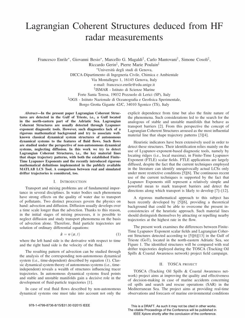
in the Western and Eastern part of the Mediterranean Sea.Gathered data are combined in a useful decision support toolfor authorities in charge of marine emergency response. Inparticular, in the GoT, which could be defined as the regionof the Adriatic Sea north-east of the ideal line connectingSavudrija and Grado, a network of three CODAR (COastalraDAR) was installed in order to measure surface velocityfields. The three radars are located in Aurisina, Barcola andPirano spots (see Figure 1). The velocity data were collectedbetween the 23rd and 30th of April 2012 with a spatialresolution of 1.5 km and a time resolution of 1 hour. In thefield campaign drifters were deployed, too. The trajectoriesof the drifters deployed in the sea were recorded thanks toGPS devices. Their positions were subsampled via kriging-interpolation methods to work with the same time resolutionof the velocity fields.

Aurisina

Barcola

Pirano

Trieste

18’

24’

13

oE

3

0.0

0’

36’

42’

48’

25’

30’

45oN

35.00’

40’

45’

Monfalcone

Fig. 1. Radar network locations in the Gulf of Trieste.

III. FINITE-TIME LYAPUNOV EXPONENTS

The detection of LCSs by FTLEs is pursued accordingto [4]. In this context FTLEs can be considered a finite-time average of the maximum expansion rate that a coupleof particles advected by the flow can experience in a finite-time interval T , called integration time. The definition of theFTLE reads

σt0+T

t0(x) =

1

|T |log

√

(λmax) (2)

where λmax is the maximum eigenvalue of the Cauchy-Greentensor, t0 is the initial time and T is the integration time,i.e., the finite-time interval over which the FTLE is calculated.Defining the deformation gradient as

F =dx(t0 + T )

dx(t0)(3)

the Cauchy-Green Tensor is evaluated as

CG = F TF . (4)

The Cauchy-Green tensor is a linear operator representedby a symmetric and positive definite matrix that expresses

a rotation-independent measure of deformation, since a purerotation does not produce any strain [14]. The FTLE valuesare computed through a finite-difference scheme [15] over aregular grid. The values associated with the nodes of the gridform a scalar field. In [4], Lagrangian Coherent Structures aredefined as the ridges of Finite-Time Lyapunov Exponent fields.

Despite several recent issues aroused around the evaluationof the flux across the ridges of FTLE fields [1] [5], a propertyhas generally been associated to these structures: the fluxacross them is very small and if they are actual LagrangianCoherent Structures the flux is null.

It is worthwhile to note that FTLEs operate with a fixedtime-scale T and detect a separation rate that changes frompoint to point. Detection of Lagrangian barriers leads to thedetection of two different types of structures that behave in op-posite ways: repelling and attractive structures are commonlypresented in literature [4][16][7]. These features are calculatedwith forward and backward particle trajectory integration intime, respectively.

IV. HYPERBOLIC LAGRANGIAN COHERENT STRUCTURES

Recent works seek Lagrangian Coherent Structures on thebasis of a rigorous mathematical formulation [1] [5] [17] [6].Over the time interval of interest the Authors define LagrangianCoherent Structures as the prevailing attracting or repellingmaterial lines. Considering a material line at the initial time,a unit normal vector n0(x0) to this line in the point x0

will change orientation over the time interval of interest andgenerally will not remain normal to the material line. Recallingthat a generic vector ξ at the initial time evolves, under thelinearized flow, into Fξ and by defining the repulsion rateρ(x0,n0) = 〈nt,Fn0〉 as the scalar product between theevolved initial unit vector Fn0 and a new unit vector nt

normal to the advected material line, it is possible to evaluatethe behaviour of the material line over the time interval ofinterest. If the repulsion rate ρ is greater than 1, the materialline will exert net normal repulsion on nearby fluid elements.On the contrary, it will exert along its normal directionattraction over the nearby fluid elements. [17] find that theinitial positions of Hyperbolic LCSs must be orthogonal to aspecific vector field. For two dimensional flows repelling LCSsmust be trajectories of the differential equation

r′ = ξ1(r) (5)

and attracting LCSs must be trajectories of the differentialequation

r′ = ξ2(r) (6)

where ξ1 and ξ2 are the eigenvectors of the Cauchy-Green ten-sor associated with the minor and the maximum eigenvalues,respectively. The numerical detection of these LCSs is carriedout by the publicly available software LCS Tool [13].

V. LAGRANGIAN COHERENT STRUCTURES IN THE GULF

OF TRIESTE

Thanks to the available velocity fields of the sea surfaceof the Gulf of Trieste, a comparison between Finite-TimeLyapunov Exponents fields and Lagrangian Coherent Struc-tures detected by LCS Tool [13] is carried out. A furtherinvestigation is developed since real drifter trajectories are

available and a direct comparison between drifters data andLCS is possible.

A. FTLE fields and Lagrangian Coherent Structures

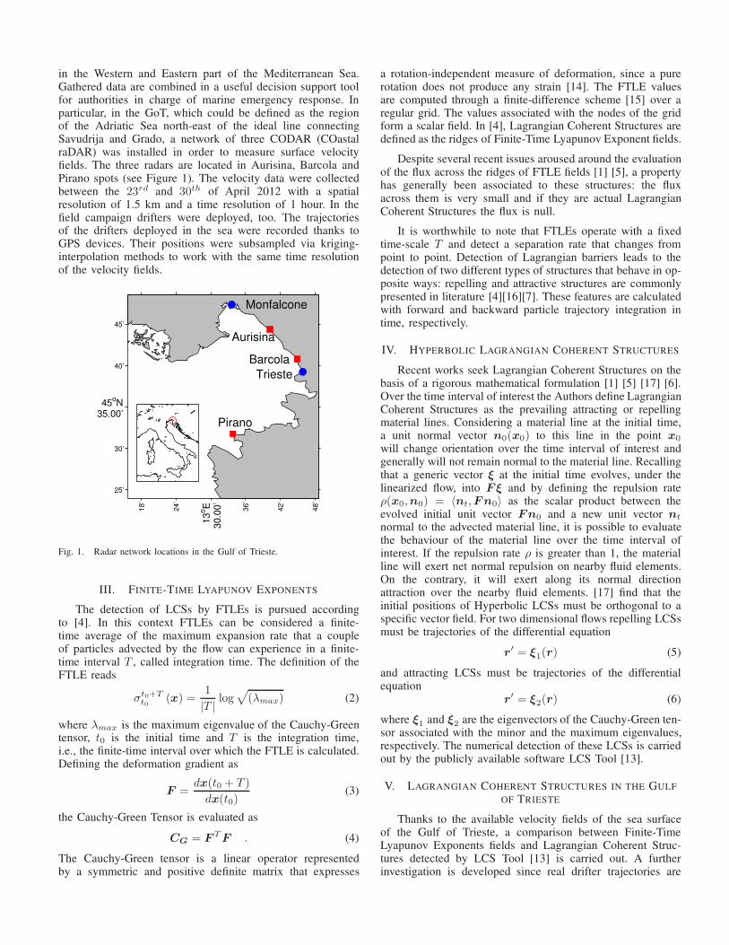
[4] associate ridges of Finite-Time Lyapunov Exponentsfields carried out with a forward integration with repellingstructures. In Figure 2 the underlying field is the FTLE forwardevaluated with an integration time T of 25 hours. The thin bluelines represent the hyperbolic repelling LCSs computed overthe same time interval calculated via the LCS Tool [13]. It ispossible to see that the ridges of the FTLE field and the LCSsdo not perfectly superimpose. A good agreement between theFTLE pattern and LCSs is present especially comparing thestructure located north-west of the GoT that closes the Gulfof Monfalcone, i.e., an internal Gulf of the GoT.

σ [

1/d

ays]

18

’

24

’

13

oE

3

0.0

0’

36

’

42

’

48

’

32’

45oN

36.00’

40’

44’

−2

−1

0

1

2

Fig. 2. Forward Finite-Time Lyapunov Exponent field for 00 UTC of the23rd of April 2012, and repelling LCSs (thin blue lines).

[18] show that ridges of FTLE coincide in many caseswell with material structures. However, in general, they arenot exact material structures, no matter which ridge definitionof a scalar field is adopted. Unless very long integration timesare used, FTLE ridges can deviate considerably from materialstructures.

Comparisons like those presented in Figure 2 could befurther investigated numerically, evaluating the flux acrossthe ridges of the scalar field and the flux across the LCSs.However, such evaluations are carried out on the basis ofvelocity fields whose reliability is taken for granted. Whetheror not ridges of FTLE fields and LCSs represent with goodapproximations material boundaries, the most important basicquestion remains: how reliable are the measured velocityfields? To address this question, in the following we comparetrajectories obtained by integrating the measured velocity fieldsand the Lagrangian real observed trajectories.

B. Drifters in the Gulf of Trieste

During the TOSCA project drifters were deployed in theGoT making possible the comparison among drifter trajectoriesand Lagrangian structures. Taking into account the trajectoryof a real drifter known with an hourly time step, it is possible tocompare such drifter trajectory and the LCS obtained with theapproaches described in Section V-A. Two types of simulations

25’

30’

13

oE

3

5.0

0’

40’

45’

32’

45oN

36.00’

40’

44’

1

10

1928

3746 55

64

Drifter 41actual drifter

simulated drifter

reseeded drifter

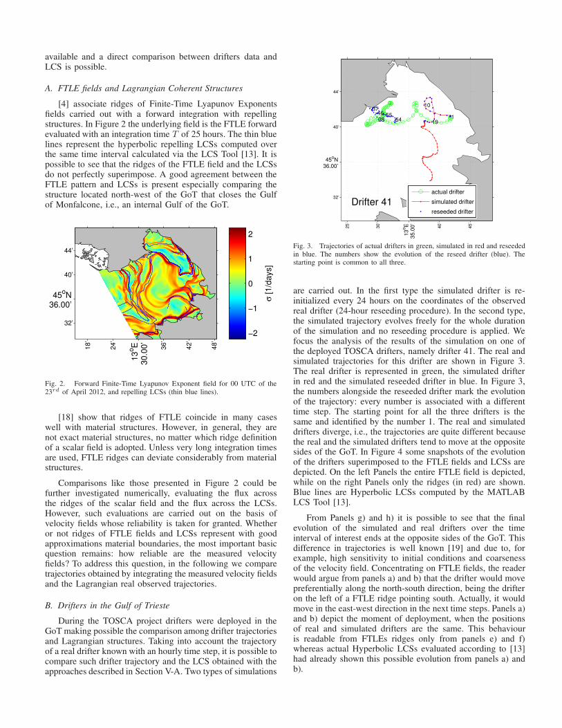
Fig. 3. Trajectories of actual drifters in green, simulated in red and reseededin blue. The numbers show the evolution of the reseed drifter (blue). Thestarting point is common to all three.

are carried out. In the first type the simulated drifter is re-initialized every 24 hours on the coordinates of the observedreal drifter (24-hour reseeding procedure). In the second type,the simulated trajectory evolves freely for the whole durationof the simulation and no reseeding procedure is applied. Wefocus the analysis of the results of the simulation on one ofthe deployed TOSCA drifters, namely drifter 41. The real andsimulated trajectories for this drifter are shown in Figure 3.The real drifter is represented in green, the simulated drifterin red and the simulated reseeded drifter in blue. In Figure 3,the numbers alongside the reseeded drifter mark the evolutionof the trajectory: every number is associated with a differenttime step. The starting point for all the three drifters is thesame and identified by the number 1. The real and simulateddrifters diverge, i.e., the trajectories are quite different becausethe real and the simulated drifters tend to move at the oppositesides of the GoT. In Figure 4 some snapshots of the evolutionof the drifters superimposed to the FTLE fields and LCSs aredepicted. On the left Panels the entire FTLE field is depicted,while on the right Panels only the ridges (in red) are shown.Blue lines are Hyperbolic LCSs computed by the MATLABLCS Tool [13].

From Panels g) and h) it is possible to see that the finalevolution of the simulated and real drifters over the timeinterval of interest ends at the opposite sides of the GoT. Thisdifference in trajectories is well known [19] and due to, forexample, high sensitivity to initial conditions and coarsenessof the velocity field. Concentrating on FTLE fields, the readerwould argue from panels a) and b) that the drifter would movepreferentially along the north-south direction, being the drifteron the left of a FTLE ridge pointing south. Actually, it wouldmove in the east-west direction in the next time steps. Panels a)and b) depict the moment of deployment, when the positionsof real and simulated drifters are the same. This behaviouris readable from FTLEs ridges only from panels e) and f)whereas actual Hyperbolic LCSs evaluated according to [13]had already shown this possible evolution from panels a) andb).

18’

24’

E

30.0

0’

36’

42’

48’

32’

45oN

36.00’

40’

44’

a)

−2

−1

0

1

2

18’

24’

E

30.0

0’

36’

42’

48’

32’

N 36.00’

40’

44’

b)

18’

24’

E

30

.00

’

36’

42’

48’

32’

45oN

36.00’

40’

44’

c)

−2

−1

0

1

2

18’

24’

E

30

.00

’

36’

42’

48’

32’

N 36.00’

40’

44’

d)

18’

24’

E

30

.00

’

36’

42’

48’

32’

45oN

36.00’

40’

44’

e)

−2

−1

0

1

2

18’

24’

E

30

.00

’

36’

42’

48’

32’

N 36.00’

40’

44’

f)

18’

24’

13

oE

3

0.0

0’

36’

42’

48’

32’

45oN

36.00’

40’

44’

g)

−2

−1

0

1

2

18’

24’

13

oE

3

0.0

0’

36’

42’

48’

32’

N 36.00’

40’

44’

h)

Fig. 4. Backward Finite-Time Lyapunov Exponent fields and attractive LCSs in blue. Real drifter in green, simulated drifter in red and simulated reseededdrifter in blue. Left Panels show the whole FTLE field and hyperpolic LCSs (thin blue lines). Right Panels show only FTLE ridges (in red) and hyperpolicLCSs (thin blue lines).

These findings suggest then that FTLE ridges can givereasonable information about the most probable direction ofspreading of passive tracers even if they are not able toreproduce accurately the information provided by LCS Tool.

VI. CONCLUSION

In this work we detected Lagrangian Coherent Structuresfrom a heuristic indicator such as Finite-Time Lyapunov Expo-nents and from a rigorous mathematical definition in the Gulfof Trieste. The input velocity fields are those measured by thenetwork of coastal radars of the TOSCA project. Lagrangianstructures are subsequently compared with field measurementsof drifter motion. A particularly interesting drifter is takeninto consideration and two different kinematic simulations arecarried out: one with a daily reseeding of the simulated drifteron the coordinates of the real one and another without reseed-ing. The trajectories are analysed at the light of the identifiedLagrangian Coherent Structures. Such an analysis shows howuseful Lagrangian structures are in studying drifter motion andunderlines that the new definitions of LCSs introduced by [5][6] could be important in finding true material lines that shapetrajectory patterns of passive tracers. However, further analysisbased on field data are to be carried out in order to assessthe reliability of LCSs to provide correct information aboutthe transport of mass in geophysical flows. Besides, furtherinvestigations are needed to assess reliability of the measuredvelocity fields.

ACKNOWLEDGMENT

The present research has been funded by Progetto diRicerca di Ateneo 2010, Universita degli Studi di Genova.Francesco Enrile has been founded by PADI Foundation grant2015. The authors gratefully acknowledge support from theMED TOSCA project, co-financed by the European RegionalDevelopment Fund. Support from the Italian Flagship ProjectRITMARE is also acknowledged.

REFERENCES

[1] G. Haller, “Lagrangian coherent structures,” Annual Review of Fluid

Mechanics, 2014.

[2] G. Boffetta, G. Lacorata, G. Redaelli, and A. Vulpiani, “Detectingbarriers to transport: a review of different techniques,” Physica D, vol.159, pp. 58–70, 2001.

[3] G. Haller, “Lagrangian structures and the rate of strain in a partitionof two-dimensional turbulence,” Physics of Fluids, vol. 13, no. 11, pp.3365–3385, 2001.

[4] S. C. Shadden, F. Lekien, and J. E. Marsden, “Definition and propertiesof lagrangian coherent structures from finite-time lyapunov exponentsin two-dimensional aperiodic flows,” Physica D, vol. 212, pp. 271–304,2005.

[5] G. Haller, “A variational theory of hyperbolic lagrangian coherentstructures,” Physica D, vol. 240, pp. 574–598, 2011.

[6] G. Haller and F. Beron-Vera, “Geodesic theory of transport barriers intwo-dimensional flows,” Physica D, vol. 240, no. 7, 2012.

[7] F. Huhn, A. von Kameke, S. Allen-Perkins, P. Montero, A. Venancio,and V. Prez-Munuzuri, “Horizontal lagrangian transport in a tidal-drivenestuary-transport barriers attached to prominent coastal boundaries,”Continental Shelf Research, vol. 39-40, pp. 1–13, 2012.

[8] M. Cencini and A. Vulpiani, “Finite size lyapunov exponent: reviewon applications,” Journal of Physics A: Mathematical and Theoretical,vol. 46, no. 4, p. 26, 2013.

[9] M. Berta, L. Ursella, F. Nencioli, A. Doglioli, A. Petrenko, andS. Cosoli, “Surface transport in the Northeastern Adriatic Sea fromFSLE analysis of HF-radar measurements,” Continental Shelf Research,vol. 77, pp. 14–23, 2014.

[10] M. Grifoll, G. Jorda, and M. Espino, “Surface water renewal and mixingmechanisms in a semi-enclosed microtidal domain. the Barcelonaharbour case,” Journal of Sea Research, vol. 90, pp. 54–63, 2014.

[11] I. Hernandez-Carrasco, V. Rossi, E. Hernandez-Garcıa, V. Garcon, andC. Lopez, “The reduction of plankton biomass induced by mesoscalestirring: A modeling study in the Benguela upwelling,” Deep Sea

Research Part I: Oceanographic Research Papers, vol. 83, pp. 65–80,2014.

[12] S. St-Onge-Drouin, G. Winkler, J.-F. Dumais, and S. Senneville, “Hy-drodynamics and spatial separation between two clades of a copepodspecies complex,” Journal of Marine Systems, vol. 129, pp. 334–342,2014.

[13] K. Onu, F. Huhn, and G. Haller, “Lcs tool: a computational platformfor lagrangian coherent structures,” arXiv:1406.3527, 2014.

[14] C. Truesdell and W. Noll, The Non-Linear Field Theories of Mechanics.Springer, 2004.

[15] S. Shadden, Lagrangian Coherent Structures. In: Roman Grigoriev,Transport and Mixing in Laminar Flows: From Microfluidics to OceanicCurrents. Wiley-VCH, 2011, pp. 59–89.

[16] I. Hernandez-Carrasco, C. Lopez, E. Hernandez-Garcıa, and A. Turiel,“How reliable are finite-size Lyapunov exponents for the assessment ofocean dynamics?” Ocean Modelling, vol. 36, no. 3, pp. 208–218, 2011.

[17] M. Farazmand and G. Haller, “Computing lagrangian coherent struc-tures from their variational theory,” Chaos, vol. 22, no. 1, 2012.

[18] T. Germer, M. Otto, R. Peikert, and H. Theisel, “Lagrangian coherentstructures with guaranteed material separation,” Eurographics / IEEE

Symposium on Visualization, vol. 30, no. 3, 2011.

[19] P. Falco, A. Griffa, P. Poulain, and E. Zambianchi, “Transport propertiesin the adriatic sea as deduced for drifter data,” Journal of Physical

Oceanography, vol. 30, pp. 2055–2017, 2000.