UNIVERSITI TEKNOLOGI MALAYSIA

UTM/RMC/F/0024 (1998)

BORANG PENGESAHAN

LAPORAN AKHIR PENYELIDIKAN

TAJUK PROJEK : DYNAMIC SCHEDULING IN A MULTI-PRODUCT MANUFACTURING SYSTEM

Saya: ASSOC. PROF. DR. ADNAN HASSAN

Mengaku membenarkan Laporan Akhir Penyelidikan ini disimpan di Perpustakaan Universiti Teknologi Malaysia dengan syarat-syarat kegunaan seperti berikut :

1. Laporan Akhir Penyelidikan ini adalah hakmilik Universiti Teknologi Malaysia.

2. Perpustakaan Universiti Teknologi Malaysia dibenarkan membuat salinan untuk tujuan rujukan sahaja.

3. Perpustakaan dibenarkan membuat penjualan salinan Laporan Akhir

Penyelidikan ini bagi kategori TIDAK TERHAD.

4. * Sila tandakan ( / )

SULIT (Mengandungi maklumat yang berdarjah keselamatan atau Kepentingan Malaysia seperti yang termaktub di dalam AKTA RAHSIA RASMI 1972). TERHAD (Mengandungi maklumat TERHAD yang telah ditentukan oleh Organisasi/badan di mana penyelidikan dijalankan). TIDAK TERHAD TANDATANGAN KETUA PENYELIDIK

Assoc. Prof. Dr. Adnan Hassan Nama & Cop Ketua Penyelidik Tarikh : _________________

CATATAN : * Jika Laporan Akhir Penyelidikan ini SULIT atau TERHAD, sila lampirkan surat daripada pihak berkuasa/organisasi berkenaan dengan menyatakan sekali sebab dan tempoh laporan ini perlu dikelaskan sebagai SULIT dan TERHAD.

Lampiran 20

VOT. 75062

DYNAMIC SCHEDULING IN A MULTI-PRODUCT MANUFACTURING SYSTEM

ASSOC. PROF. DR ADNAN HASSAN

PROF. DR. AWALUDDIN MOHD SHAHAROUN MUCHAMAD OKTAVIANDRI

RESEARCH VOT NO. 75062

Dept. of Manufacturing and Industrial Engineering Faculty of Mechanical Engineering

Universiti Teknologi Malaysia

2007 20

07

Facu

lty o

f Mec

hani

cal E

ngin

eerin

g D

ept.

of M

anuf

actu

ring

and

Indu

stria

l Eng

inee

ring

Ass

oc. P

rof.

Dr.

Adn

an H

assa

n Pr

of. D

r. A

wal

uddi

n M

ohd

Shah

arou

n M

ucha

mad

Okt

avia

ndri

Dyn

amic

Sch

edul

ing

in a

Mul

ti-Pr

oduc

t Man

ufac

turin

g Sy

stem

VO

T 7

5062

VOT. 75062

DYNAMIC SCHEDULING IN A MULTI-PRODUCT MANUFACTURING SYSTEM

ASSOC. PROF. DR ADNAN HASSAN

PROF. DR. AWALUDDIN MOHD SHAHAROUN MUCHAMAD OKTAVIANDRI

RESEARCH VOT NO. 75062

Dept. of Manufacturing and Industrial Engineering Faculty of Mechanical Engineering

Universiti Teknologi Malaysia

2007

Ass

oc. P

rof.

Dr.

Adn

an H

assa

n Pr

of. D

r. A

wal

uddi

n M

ohd

Shah

arou

n M

ucha

mad

Okt

avia

ndri

Dyn

amic

Sch

edul

ing

in a

Mul

ti-Pr

oduc

t Man

ufac

turin

g Sy

stem

Fa

culty

of M

echa

nica

l Eng

inee

ring

Dep

t. of

Man

ufac

turin

g an

d In

dust

rial E

ngin

eerin

g 20

07

DYNAMIC SCHEDULING IN A MULTI-PRODUCT MANUFACTURING SYSTEM

(Keywords: dynamic scheduling, job shop, ANN model, simulation scheduling)

To remain competitive in global marketplace, manufacturing companies need to improve their operational practices. One of the methods to increase competitiveness in manufacturing is by implementing proper scheduling system. This is important to enable job orders to be completed on time, minimize waiting time and maximize utilization of equipment and machineries. The dynamics of real manufacturing system are very complex in nature. Schedules developed based on deterministic algorithms are unable to effectively deal with uncertainties in demand and capacity. Significant differences can be found between planned schedules and actual schedule implementation. This study attempted to develop a scheduling system that is able to react quickly and reliably for accommodating changes in product demand and manufacturing capacity. A case study, 6 by 6 job shop scheduling problem was adapted with uncertainty elements added to the data sets. A simulation model was designed and implemented using ARENA simulation package to generate various job shop scheduling scenarios. Their performances were evaluated using scheduling rules, namely, first-in-first-out (FIFO), earliest due date (EDD), and shortest processing time (SPT). An artificial neural network (ANN) model was developed and trained using various scheduling scenarios generated by ARENA simulation. The experimental results suggest that the ANN scheduling model can provided moderately reliable prediction results for limited scenarios when predicting the number completed jobs, maximum flowtime, average machine utilization, and average length of queue. This study has provided better understanding on the effects of changes in demand and capacity on the job shop schedules. Areas for further study includes: (i) Fine tune the proposed ANN scheduling model (ii) Consider more variety of job shop environment (iii) Incorporate an expert system for interpretation of results. The theoretical framework proposed in this study can be used as a basis for further investigation.

Key Researchers:

Assoc. Prof. Dr. Adnan Hassan

Prof. Dr. Awaluddin Mohd Shaharoun Muchamad Oktaviandri

E-mail : Adnan@fkm.utm.my Tel. No. : 07-5534850 Vote No.: 75062

TABLE OF CONTENTS

CHAPTER TITLE

ABSTRACT ii

TABLE OF CONTENTS iii

LIST OF TABLES vi

LIST OF FIGURES viii

LIST OF APPENDICES ix

CHAPTER 1 INTRODUCTION

1.1 Background of the Problem 1

1.2 Statement of the Problem 3

1.3 Objectives of the Study 4

1.4 Scope of the Study 4

1.5 Importance of the Study 4

1.6 Organization of the Report 5

CHAPTER 2 LITERATURE REVIEW

2.1 Scheduling 6

2.1.1. Introduction 6

2.1.2. Notation for Scheduling 9

2.1.3. Scheduling Classification 11

2.1.4. Scheduling Complexity 16

2.1.5 Scheduling Rules 19

2.1.6 Performance Measures 20

2.2. Job Shop Scheduling 22

2.3. Dynamic Scheduling 24

iv

2.3.1. The Dynamic Job shop Scheduling Characteristics 25

2.3.2 Previous Research on Dynamic Scheduling 26

2.3.3 Dynamic Scheduling Approaches 29

2.4 Simulation In Scheduling 31

2.4.1 Motivation for Simulation 33

2.4.2 The Steps of Simulation 34

2.4.3 Scheduling Through Simulation 37

2.5 Design of Simulation Experimentation 37

2.5.1 Order Arrivals 38

2.5.2 Processing and Setup Times 40

2.5.3 Number of Machines 41

2.5.4 Job Routing 42

2.5.5 Machine and Shop Utilization 43

2.5.6 Due Date 43

2.5.7 Priority Rules 44

2.6 Simulation and Its Application on Scheduling 46

2.5 ANN for Solving Scheduling Problems 48

2.5 Summary of Chapter 2 50

CHAPTER 3 RESEARCH METHODOLOGY

3.1 Traditional and Proposed Framework 52

3.2 Operational Framework 54

3.3 Research Questions 55

3.4 Development Phases 56

CHAPTER 4 MODEL DEVELOPMENT

4.1 Problem Definition and Training Samples Generation 57

4-2 Simulation Model 59

4.2.1 Steady-state Condition of the Shop (Warm up period) 594.2.2 Run Length and Number of Replications 60

4.3 ANN Model 604.4 Sequences Codification Scheme 62

v

CHAPTER 5 RESULTS AND DISCUSSION 5.1 Simulation Results 635.2 ANN Training Results 63

5.2.1 Parameter Used in the BP-MLP 5.2.2 The Training Convergent Curve

5-3 Comparison Between Simulation Results and Predict Results 735.4 Discussions 78 CHAPTER 6 CONCLUSSIONS 83 REFFERENCES 84 APPENDICES

vi

LIST OF TABLES

Table 2.1 Description of Topics Covered by Reviews Articles in

Scheduling.

7

Table 2.2 Classifies the Articles by Topics. 8

Table 2-3 Advantages and Disadvantages of Simulation 32

Table 2-4 Capabilities and Limitations of Simulation 32

Table 4-1 Original data of 6 X 6 job shop scheduling problem from

Fisher and Thompson (1963).

57

Table 5-1 Result from Simulation, Scheduling Rule = FIFO, Job Arrival

= “Low”

64

Table 5-2 Result from Simulation, Scheduling Rule = EDD, Job Arrival

= “Low”

65

Table 5-3 Result from Simulation, Scheduling Rule = SPT, Job Arrival

= “Low”

66

Table 5-4 Result from Simulation, Scheduling Rule = FIFO, Job Arrival

= “Medium”

67

Table 5-5 Result from Simulation, Scheduling Rule = EDD, Job Arrival

= “Medium”

68

Table 5-6 Result from Simulation, Scheduling Rule = SPT, Job Arrival

= “Medium”

69

Table 5-7 Result from Simulation, Scheduling Rule = FIFO, Job Arrival

= “High”

70

Table 5-8 Result from Simulation, Scheduling Rule = EDD, Job Arrival

= “High”

71

Table 5-9 Result from Simulation, Scheduling Rule = SPT, Job Arrival

= “High”

72

Table 5-10 Training Parameters . 73

vii

Table 5-10 Training Parameters . 73

Table 5.11 Comparison of Number Completed Jobs. 74

Table 5.12 Comparison of Maximum Flowtime Job 75

Table 5.13 Comparison of Average Machine Utilization 76

Table 5.14 Comparison of Average Job Q Length for the Machine 77

viii

LIST OF FIGURES

Figure 1-1: Summary Background of the problems. 2

Figure 2-1, Models of Machine Configuration 13

Figure 2.3, Flow Shops, Open Shops, and Job Shops. 15

Figure 2-4, Simulation Modeling Processes 34

Figure 3-1: Traditional Theoretical Framework 53

Figure 3-2: Proposed Theoretical Framework 54

Figure 3-3: Operational Framework 55

Figure 3-4: Development Phases 56

Figure 4-1: Physical configuration of a six-machine dynamic job shop. 58

Figure 4-2, ANN Schedule Model 61

Figure 4-3, Error Adjusted for ANN model. 61

Figure 5-1: Mean Absolute Error Convergent curve of Training 73

Figure 5.2 Comparison of Number Completed Jobs. 79

Figure 5.3 Comparison of Maximum Flowtime Job 80

Figure 5.4 Comparison of Average Machine Utilization 81

Figure 5.5 Comparison of Average Job Q Length for the Machine 82

ix

LIST OF APPENDICES

APPENDIX A: Most Common Scheduling Rules 93

APPENDIX B: FIFO, SPT and EDD Algorithm 94

Appendix C: Most Common Performance Measure 97

APPENDIX D: Summary for Result from Simulation where Scheduling Rule

= FIFO, Job Arrival = “Low”

98

APPENDIX E: Sequences Codification Scheme 108

CHAPTER 1

INTRODUCTION

1.1 Background of the problem

The effect of globalization in every sector of the country, such as economic,

information technology, communication, transportation, etc. has directly heightened

customer expectation. Today’s customers expect to be delighted with customized

quality, lower price, time delivery, and service satisfaction. These situations have

forced manufacturers to adapt changes in technology, among others, automated,

flexibility and integrated system, rapid and short run manufacturing have been

improved to respond customer expectation (Hassan, 2002). Figure 1.1 summarizes

the background of the problems. Frequent changes due to the above mentioned

factors have meant frequent rescheduling of production operation. Flexibility in

reacting to changes in production scheduling has become an important attribute of

modern manufacturing system.

One method of increasing the productivity of a manufacturing is by proper

production scheduling of the jobs on the available machines/resources so that a high

percentage of orders can be completed on time, average waiting time of orders

minimized and utilization of the equipment maximized. The production schedulers

(people who make scheduling) have to make a production schedule to meet shorten

production lead time, to reduce work-in-process (WIP) inventory and to improve

machine utilization. Even if he/she has special knowledge and experience for shop

floor control, the scheduling job is much too complicated and time-consuming. To

2

solve these problems, schedulers have to use more effective and interactive

production schedules.

Figure 1.1: Background of the problems.

There is always some degree of uncertainty present in the real manufacturing

environment that can affect the reliability of any production schedule. When these

dynamic events occur, the current schedule that uses some static assumption will no

longer be considered optimal. Therefore, robust scheduling systems are desirable to

be used in the manufacturing process.

The dynamics of real manufacturing system are very complex in nature.

Schedule based on deterministic algorithms fail to deal with any disturbances, such

Globalization Economic, Information

Technology, Communication, Transportation, etc

Challenge in manufacturing system Order that are released in a manufacturing setting have to be translated into jobs with

associated due dates. These jobs often have to be processed on the machines in a workcenter

in a given order or sequence

The Problem Production Scheduling need to address dynamic changes in production capacity and changes in customer demand..

Improvement

Changes in manufacturing

Automated, Flexible and Integrated, Rapid and short run manufacturing

Trend in customer demand Customized quality, lowest

price, timely delivery and delightful service.

Dynamic and unexpected demand

Pressures

Response

Requires

“Uncertainty”

3

uncertainties as changes in demand and capacity. Significant differences can be

found between planned schedules and actual process in progress. Based on this

background, this study attempted to develop a production scheduling system that is

able to react quickly, reliably, and can accommodate changes in demand and

capacity.

1.2 Statement of the problem

Although most manufacturing scheduling problems are dynamic and

stochastic in nature, the majority of available scheduling techniques are based on

static and deterministic conditions. This is partly due to the difficulty in formulating

and solving dynamic problems analytically. As a consequence, the solutions obtained

from the traditional scheduling technique fail wherever changes occur to the system

(Vieira, 2000).

Changes in manufacturing system can be defined as deviations which occur

during production that cause such systems to behave differently from what is

expected (Pendharkar, 1999). Changes can cause the scheduling system to perform

its function either incorrectly or inefficiently. As a result, the changes can eventually

prevent the system from accomplishing its objective or delivering products to

customer on time. Changes in manufacturing can be classified into two broad

categories (Vieira, 2000); (i) changes in demand, such as rush job, job cancellation

by customer and changes in master production schedule, (ii) changes in capacity,

such as unplanned machine breakdowns, illness of manpower and maintenance.

Managing such changes is becoming critical in the era of time-based competition.

For example, if a schedule is generated without considering possible orders in the

future, new orders of significant urgency may interrupt those already scheduled,

causing serious violation of their promised delivery dates. When this dynamic event

occurs, the current schedule that uses some static assumption is no longer optimal.

4

1.3 Objectives of the Study

The research objectives are listed as below:

(i) To compare effectiveness of various scheduling rules in dynamic job shop

scheduling.

(ii) To develop a decision support model for enabling analysis of dynamic

scheduling of job shops under conditions of changing demand and/or

capacity.

1.4 Scope of the study

The scope of research is limited to job shops, when jobs arrive in the shop in

a dynamic and random manner to the scheduler.

• The study is limited to discrete products.

• Focusing on small and medium industries (SMI).

• The performance measures are limited to three: (i) minimization of

the makespan, (ii) minimization of average tardiness and (iii)

minimization of percentage number of tardy jobs

1.5 Importance of the study

The study is important and significant both from the theoretical and practical

view point. The rationale and motivation for this study are:

(i). Traditionally, majority of current scheduling research assume static

and deterministic condition, whereas, real manufacturing system are

dynamic and stochastic in nature.

(ii). This study addresses small and medium sized industries, and aimed at

non-specialist scheduler. Such people normally built a schedule from

scratch to address a particular job, and then it is often discarded/

5

forgotten. This approach is very expensive, time consuming, and

wasteful. There is a need for a schedule system that retains and builds

on existing knowledge and be used as a predictive tool when

unforeseen and dynamic changes occur to the manufacturing system

1.6 Organization of the Report

This report is organized into 6 chapters. Chapter 1 serve as an essential

introduction to the research. Chapter 1 provides background information and a

review of related literature that leads to the formulation of this report. Chapter 1

describes the research methodology and its rationale. Chapter 4 describes models

development. Chapter 5 presents the data result and discussion. Chapter 5 provides

an overall conclusion and suggestions for future research.

CHAPTER 2

LITERATURE REVIEW

2.1 Scheduling

2.1.1. Introduction

Scheduling deals with the allocation of scarce resources to task over time. It

is a decision-making process with the goal of optimizing one or more objectives

(Pinedo, 2002). Scheduling is important issue in management of organizations

because it determines the cost and services reputation of the company with respect to

the competition. The need to respond to market demand quickly and run plants

efficiently raises complex scheduling problems in almost all but the simplest

production environments.

The theory of scheduling has received significant attention since its beginning

in the early 1950. A representative, although not complete, list of the most important

survey on the field are: (Graves, 1981), ( Sen and Gupta, 1984) (Ramashes, 1990),

(Sevastjanov, 1994), (Nagar, 1995), (Blazewick et al., 1996) (Hall, 1996), (Drexl,

1997), (Mokotoff, 2001) and (Raheja and Subramaniam, 2002), (Lee et. al, 1997) .

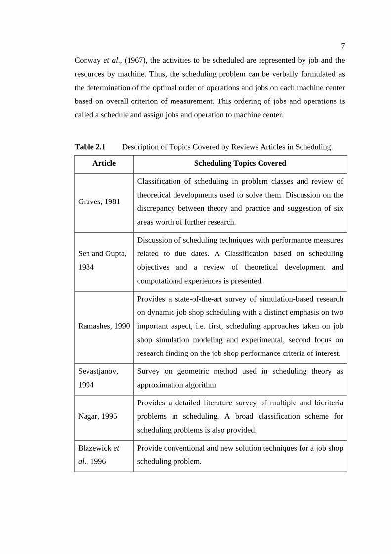
Table 2.1 provides a brief summary of the topics covered by each article, while Table

2.2 classifies the articles by topics.

In additional, (Conway, et al., 1967), (Baker, 1974) ), (Rinooy Kan, 1979),

(Gupta, 1981), (French, 1982), (Blazewicz, et al, 1993), (Brucker, 1995), (Jordan,

1996), ( Kimms, 1997), (Pinedo, 2002), and (Cottet, 2002) are book containing most

of the basic theoretical knowledge accumulated to date. Partly under the influence of

7

Conway et al., (1967), the activities to be scheduled are represented by job and the

resources by machine. Thus, the scheduling problem can be verbally formulated as

the determination of the optimal order of operations and jobs on each machine center

based on overall criterion of measurement. This ordering of jobs and operations is

called a schedule and assign jobs and operation to machine center.

Table 2.1 Description of Topics Covered by Reviews Articles in Scheduling.

Article Scheduling Topics Covered

Graves, 1981

Classification of scheduling in problem classes and review of

theoretical developments used to solve them. Discussion on the

discrepancy between theory and practice and suggestion of six

areas worth of further research.

Sen and Gupta,

1984

Discussion of scheduling techniques with performance measures

related to due dates. A Classification based on scheduling

objectives and a review of theoretical development and

computational experiences is presented.

Ramashes, 1990

Provides a state-of-the-art survey of simulation-based research

on dynamic job shop scheduling with a distinct emphasis on two

important aspect, i.e. first, scheduling approaches taken on job

shop simulation modeling and experimental, second focus on

research finding on the job shop performance criteria of interest.

Sevastjanov,

1994

Survey on geometric method used in scheduling theory as

approximation algorithm.

Nagar, 1995

Provides a detailed literature survey of multiple and bicriteria

problems in scheduling. A broad classification scheme for

scheduling problems is also provided.

Blazewick et

al., 1996

Provide conventional and new solution techniques for a job shop

scheduling problem.

8

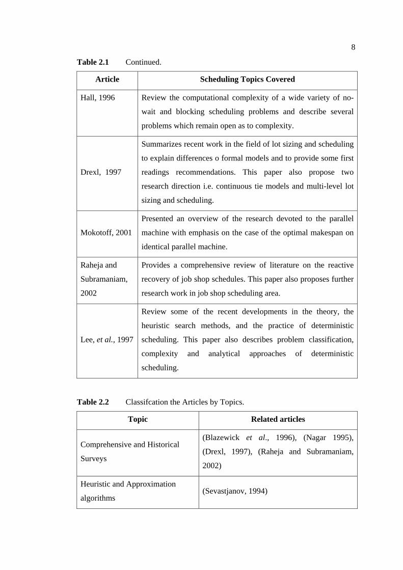
Table 2.1 Continued.

Article Scheduling Topics Covered

Hall, 1996 Review the computational complexity of a wide variety of no-

wait and blocking scheduling problems and describe several

problems which remain open as to complexity.

Drexl, 1997

Summarizes recent work in the field of lot sizing and scheduling

to explain differences o formal models and to provide some first

readings recommendations. This paper also propose two

research direction i.e. continuous tie models and multi-level lot

sizing and scheduling.

Mokotoff, 2001

Presented an overview of the research devoted to the parallel

machine with emphasis on the case of the optimal makespan on

identical parallel machine.

Raheja and

Subramaniam,

2002

Provides a comprehensive review of literature on the reactive

recovery of job shop schedules. This paper also proposes further

research work in job shop scheduling area.

Lee, et al., 1997

Review some of the recent developments in the theory, the

heuristic search methods, and the practice of deterministic

scheduling. This paper also describes problem classification,

complexity and analytical approaches of deterministic

scheduling.

Table 2.2 Classifcation the Articles by Topics.

Topic Related articles

Comprehensive and Historical

Surveys

(Blazewick et al., 1996), (Nagar 1995),

(Drexl, 1997), (Raheja and Subramaniam,

2002)

Heuristic and Approximation

algorithms (Sevastjanov, 1994)

9

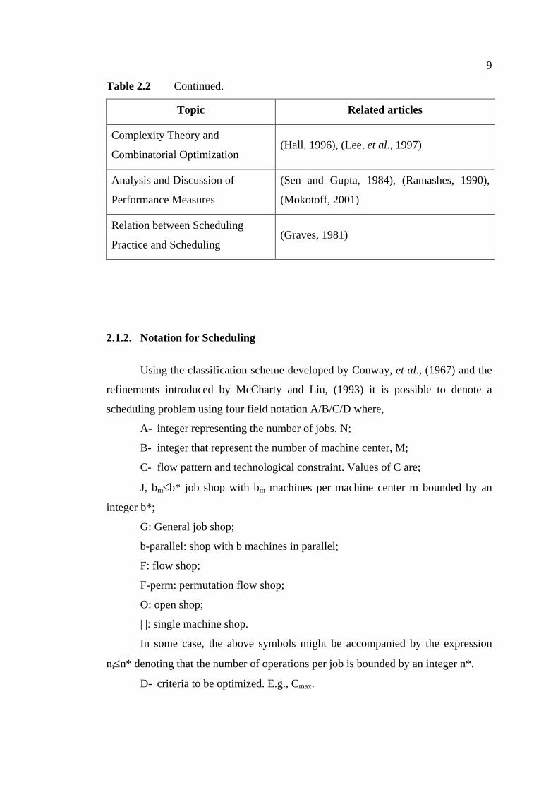
Table 2.2 Continued.

Topic Related articles

Complexity Theory and

Combinatorial Optimization (Hall, 1996), (Lee, et al., 1997)

Analysis and Discussion of

Performance Measures

(Sen and Gupta, 1984), (Ramashes, 1990),

(Mokotoff, 2001)

Relation between Scheduling

Practice and Scheduling (Graves, 1981)

2.1.2. Notation for Scheduling

Using the classification scheme developed by Conway, et al., (1967) and the

refinements introduced by McCharty and Liu, (1993) it is possible to denote a

scheduling problem using four field notation A/B/C/D where,

A- integer representing the number of jobs, N;

B- integer that represent the number of machine center, M;

C- flow pattern and technological constraint. Values of C are;

J, bm≤b* job shop with bm machines per machine center m bounded by an

integer b*;

G: General job shop;

b-parallel: shop with b machines in parallel;

F: flow shop;

F-perm: permutation flow shop;

O: open shop;

| |: single machine shop.

In some case, the above symbols might be accompanied by the expression

ni≤n* denoting that the number of operations per job is bounded by an integer n*.

D- criteria to be optimized. E.g., Cmax.

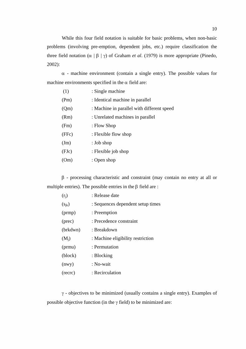
10

While this four field notation is suitable for basic problems, when non-basic

problems (involving pre-emption, dependent jobs, etc.) require classification the

three field notation (α | β | γ) of Graham et al. (1979) is more appropriate (Pinedo,

2002):

α - machine environment (contain a single entry). The possible values for

machine environments specified in the α field are:

(1) : Single machine

(Pm) : Identical machine in parallel

(Qm) : Machine in parallel with different speed

(Rm) : Unrelated machines in parallel

(Fm) : Flow Shop

(FFc) : Flexible flow shop

(Jm) : Job shop

(FJc) : Flexible job shop

(Om) : Open shop

β - processing characteristic and constraint (may contain no entry at all or

multiple entries). The possible entries in the β field are :

(rj) : Release date

(sjk) : Sequences dependent setup times

(prmp) : Preemption

(prec) : Precedence constraint

(brkdwn) : Breakdown

(Mj) : Machine eligibility restriction

(prmu) : Permutation

(block) : Blocking

(nwy) : No-wait

(recrc) : Recirculation

γ - objectives to be minimized (usually contains a single entry). Examples of

possible objective function (in the γ field) to be minimized are:

11

• Makespan (Cmax)

• Maximum Lateness (Lmax)

• Total weighted completion time (∑ )( jj Cw )

• Discounted total weighted completion times ( )1( rCjj ew −−∑ )

• Total weighted tardiness ( jjTw∑ )

• Weighted number of tardy jobs ( jjUw∑ )

MacCarthy and Liu (1993) indicate that the four field technique has been

widely used and is familiar to most schedule researches. Consequently they propose

a combination of the two methods where the C field is modified to take into account

non-basic models.

2.1.3. Scheduling Classification

Scheduling problems can be classified in many ways, such as base on job

arrival, information flow to the scheduler, production stages, resources configuration

and flexibility of resources (Bongaerts, 1998, French, 1982).

a. Based on Job Arrival

According to availability of jobs prior to the creation of the schedule,

scheduling system can be classified as static and dynamic. In static scheduling all

jobs are identified when creating the scheduling, and once the production sequences

are defined, they are assumed not to be changes during processing. In dynamic

scheduling, jobs arrive dynamically over time and are scheduled after arrival.

12

b. Based on Information to the Scheduler

Base on information to the scheduler, scheduling system can be classified as

Deterministic or stochastic. When processing times and all other parameter are

known and fixed, we call our problems deterministic. Problems, which the

processing times, etc. is uncertain, are called stochastic.

c. Processing Complexity

Processing complexity refers to the number of processing steps and

workstation associated with the production process. This dimension can be

decomposed further as follows:

1. One stage, one machine,

2. One stages, multiple machine,

3. Multistage, flow shop,

4. Multistage, job shop.

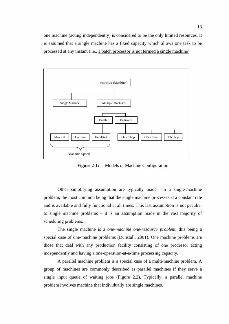
d. Based on Resources Configuration

Base on models of Machine arrangement, the following scheduling problems

can be defined (Blazewick et al., 1994) as shown as Figure 2.1. Base on

layout/configuration of the machines (Figure 2.1), the following scheduling problems

can be defined:

Single machine model (French, 1982) has the simplest layout. It consists of a

single machine that performs all operations. For models of machine in scheduling,

the single machine model represents the simplest case. In a single machine problem,

13

one machine (acting independently) is considered to be the only limited resources. It

is assumed that a single machine has a fixed capacity which allows one task to be

processed at any instant (i.e., a batch processor is not termed a single machine)

Figure 2-1: Models of Machine Configuration

Other simplifying assumption are typically made in a single-machine

problem, the most common being that the single machine processes at a constant rate

and is available and fully functional at all times. This last assumption is not peculiar

to single machine problems – it is an assumption made in the vast majority of

scheduling problems.

The single machine is a one-machine one-resource problem, this being a

special case of one-machine problems (Dunstall, 2001). One machine problems are

those that deal with any production facility consisting of one processor acting

independently and having a one-operation-at-a-time processing capacity.

A parallel machine problem is a special case of a multi-machine problem. A

group of machines are commonly described as parallel machines if they serve a

single input queue of waiting jobs (Figure 2.2). Typically, a parallel machine

problem involves machine that individually are single machines.

Processor (Machine)

Parallel

Flow Shop

Dedicated

Identical Job Shop Open Shop Uniform Unrelated

Multiple Machines Single Machine

Machine Speed

14

There are three basic types of parallel machines modeled in scheduling

problems: identical parallel machines, uniform or proportional parallel machines, and

unrelated parallel machines. In a problem with identical parallel machines, all

machine operate at the same speed (processing rate) and have the same processing

capabilities. Uniform machines have the same processing capabilities but each has a

different processing rate.ρm (ρm > 0, 1 ≤ m ≤ M), with the processing time of job j on

machine m given by processing rate Ρmj = Ρj/ρm for a given processing requirement

for Ρj job aj.

Unrelated parallel machine represent the most complex of the three standards

parallel machine type; such machine do not necessarily have identical processing

capabilities, and the processing time of each job on machine m need not be related to

either the processing times of other jobs on the same machine or to the processing

time required on other machines. For each job j and machine m, a “job-dependent

speed” Ρmj is specified and used to provide processing time Ρmj = Ρj/ρmj. If a job

cannot be processed on a certain machine, the use of value of ρmj “near to zero” can

Figure 2.2: A Representation of Parallel Machine and a Single Input Queue.

Queue of Waiting Jobs

Machine 1

Machine 2

Machine M

A Group of Machines

15

prohibit the job from being scheduled on that machine, due to the extraordinarily

large processing time assigned to it.

An interesting extension to the “standard” parallel machine model is the

parallel multi-purpose machine models. Each job or operation of a job can be

processed on a particular subset of the parallel machines, and the parallel machines

are otherwise either identical or uniform. Only a small amount of scheduling research

has been directed toward multi-purpose machine models, although interested readers

are referred to (Brucker, 1995), for example.

Single and parallel machines can be seen as representing individual

processing units, or workcenters, in a plant. Where the execution of entire

workorders (i.e., all operation of a job) can be carried out on one workcenter, these

machine models can incorporate almost all of the relevant machine characteristics.

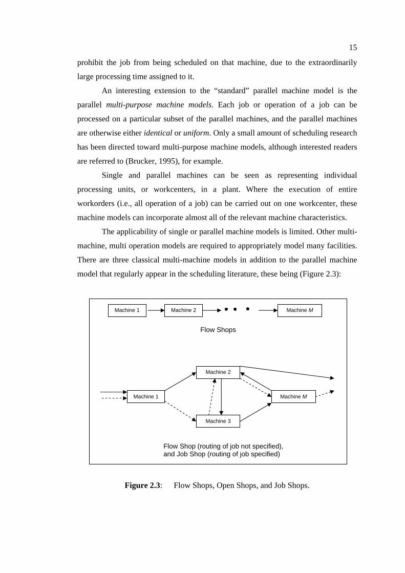
The applicability of single or parallel machine models is limited. Other multi-

machine, multi operation models are required to appropriately model many facilities.

There are three classical multi-machine models in addition to the parallel machine

model that regularly appear in the scheduling literature, these being (Figure 2.3):

Figure 2.3: Flow Shops, Open Shops, and Job Shops.

Flow Shop (routing of job not specified), and Job Shop (routing of job specified)

Flow Shops

Machine 1 Machine 2 Machine M

Machine 2

Machine 1

Machine 3

Machine M

16

• Flow shop, where all work flows from one machine (workcenter) to

the next; that is job share a common operation (processing) order and hence a

common routing through the shop. A flow shop model implies that chain precedence

holds between the operations of each job. In simple word, flow shop is a model,

where every job visits several machines, but all job have same sequence

• Job shop, where operations of a job must be carried out in

prespecified order (chain precedence) and on a prespecified machine (or parallel

machines), so that individual job routings are fixed, but can vary between jobs. In

simple word job shop is a model, where every job visits several machines, but with

dependent sequence and routing specified;

• Open Shops, Where restrictions are not placed on the operation order

(no precedence). Job routings are part of the decision process, but operation-machine

assignments are predetermined. In simple word, open shop is a model, where every

job visits several machines, but with dependent sequence and routing not specified;

Some multi-machine environments will be inadequately represented within

the classical classification scheme of flow shop, open shops, and job shops. For the

purpose of this chapter, however, there is no need to extend the classification.

2.1.4. Scheduling Complexity

The theory of computational complexity can be traced back to the works of

and (Karp, 1972) who first studied the relation between the classes P and NP of

language recognition problems solvable by deterministic and non deterministic

Turing machine respectively. This language recognition problem can be solved in a

number of steps bounded by a polynomial function in the length of the input. With

respect to combinatorial optimization, where deterministic scheduling problems

belong, a rigorous mathematical definition of concepts is not needed (Lenstra, et. al.

1977), and it is sufficient to identify with P the class problems for which a

polynomial-bounded, good or efficient algorithm exist (Edmon, 1965). On the other

hand, all problems in NP can be solved by polynomial-depth backtrack search.

17

In the original context of complexity theory, all problems are stated in term of

recognition problems which require a yes/no answer. To deal with the complexity of

a combinatorial minimization problem, a transformation into the problem of

determining the existence of a solution with value at most equal to z, for some

threshold value z, is needed.

Problems in NP are not all equal in term of computational difficulty. It is

clear that P⊂NP, but the proper inclusion is not yet known to be true or false. In fact

one of the most intriguing open question is whether or not P=NP.

There are some problems of the NP class, however, that are considering the

most difficult ones.

This is the NP-complete class. To clearly define this class, one must first

define a problem P’ as being reducible to a problem P. denoted P’∝P, if for any

instance of P’ an instance of P can be constructed in polynomial-bounded time such

that solving the instance of P will solve the instance of P’ instance. P is called NP-

hard if P’∝P ∀P’∝NP, and P is NP-complete if P is NP-hard and P ∉NP (Lenstra

and Rinnooy Kan 1979). The theory of NP-completeness provides many

straightforward techniques for proving that a given problem is “just as hard” as a

large number of other “very difficult” problems. Thus, the theory of NP-

completeness assists designers of algorithms in directing their problem solving

efforts toward those approaches that have the greatest likelihood of leading to useful

algorithms (Garey and Johnson, 1979).

Establishing NP-completeness for a scheduling problem is a strong

justification for the use of enumerative methods, since no better optimal algorithm is

likely to exist. (Graham, et. al., 1979) have catalogued approximately 9.000

scheduling problems according to their computational complexity. Roughly 9% of

these are P, 77% are NP-hard, and the remaining 14% are open. (Legeweg, et. al.,

1981) describe a computer program that maintains a record of the known complexity

results for a structured class of combinatorial problems. Given listing of well-solved

and NP-hard problems, the program employs a reducibility relation defined on the

class to classify each problems s easy, hard or open and to open one, the hardest open

ones and the easiest hard ones. The program was applied to class of 4536 machine

18

problems. The result indicates that 416 (9%) are P, 3730 (82%) are NP-hard, and the

remaining 390 (8%) are still open (Lenstra and Rinnoy Kan 1984, 1985).

From a practical point of view, in order to solve NP-hard and NP-complete

problems there is a need to:

(1) relax some of the constraints;

(2) use approximation algorithms and/or heuristics, and;

(3) use exact exponential algorithms.

Relaxation for scheduling problems is concerned with task preemptions, unit

processing times, weaker precedence constraints, etc. The use of approximation

algorithm requires an analysis of the quality of the solutions, where the distance to

the optimum may be evaluated either in the worst case or on the average (Feisher,

1980). In the case of heuristic, a benchmark of problems might be used to suggest

performance on practice with respect to parameters describing specific instances of

the heuristic. Exact exponential algorithm are used mainly for small instances of the

problem or for solving problems of special structure (blazewicz, et. al., 1988).

To further limit the complexity of the problem, the following assumptions are

made for the models development below:

1. Each job, denoted by a work order, is an entity;

2. No pre-emption;

3. Each job has m distinct operations, one on each machine;

4. No cancellation;

5. The processing times are independent of the schedule;

6. In-process inventory is allowed;

7. There is only one of each type of machine;

8. Machine may be idle;

9. No machine may process more than one operation at time;

10. Machines never break down, and are available throughout the

scheduling period;

11. The technological constraint are known in advance and are

immutable;

12. There is no randomness, in particular:

The number of jobs is known and fixed,

19

The number of machines is known and fixed,

The processing times are known and fixed,

The ready times are known and fixed,

All other quantities needed to define a particular problem are

known and fixed.

There are standard assumption in job shop research ((Baker, 1974), (Conway,

et. al., 1967), (Blazewicz, et. al. 1993)), and obey to historical reasons based on the

need for simple models that can capture the essence of a scheduling problems very

difficult to solve if all possible variables that influence it are considered ((Sisson,

1959), (Mellor, 1966), and (Gere 1966)). Even though these assumption have been

challenged on the basis of generalization an lack of applicability to real scheduling

problems, it is also true that for most practical problems it is sufficient to get good

suboptimal solution and, therefore, theoretical work and development of heuristic on

simple models is still needed (Kan, 1979)

2.1.5 Scheduling Rules

A scheduling rule is used to select a job to be processed from a set of jobs

waiting for services (these rules can also be used to introduce workpieces into the

system, to route the parts in the system and also to assign parts to facilities).

Scheduling rules may be static or dynamic. Because of the large number of

scheduling rules, it is not obvious which scheduling rule to select in a given

environment. However, have shown that the selection of the scheduling rules can

have a significant impact on system performance. Hence, in recent years, substantial

research and study has been carried out in analyzing these scheduling rules (Table 3).

20

2.1.6 Performance Measures

A variety of performance measures guide rescheduling. These measures can be

separated into three groups (Jain and Elmaraghy, 1997; Shafaei, and Brunn, 1999;

Wu, Storer, and Chang, 1993): measures of schedule efficiency, measures of

schedule stability, and cost.

Measures of schedule efficiency are often used when generating a production

schedule. They are generally time-based measures (Shafaei and Brunn, 1999):

makespan (Yamamoto, and Nof, 1985; Sabuncuoglu, and Karabuk, 1999; Fang, and

Xi, 1997; Wu, Storer,and Chang, 1993), mean tardiness (Jain and Elmaraghy, 1997

Sabuncuoglu and Karabuk, 1999), mean flow-time (Jain and Elmaraghy, 1997),

average resource utilization (Jain and Elmaraghy, 1997), and maximum lateness

(Church and Uzsoy, 1992).

Schedule stability is not an issue in static, deterministic rescheduling

environments since the schedule does not need updating. However, in other

rescheduling environments, stability, nervousness, and robustness are important

measures. Wu, Storer and Chang (1993), for instance, have said that the impact of

schedule change is a non-regular performance measure defined in two ways: (1) the

starting time deviations between the new schedule and the original schedule, and (2)

a measure of the sequence difference between the two schedules. Abumaizar and

Svestka (1997) proposed similar ideas saying that measures of stability deal with

deviation from the initial schedule. Watatani and Fujii (1992) and Dhingra, Musser

and Blankenship (1992) also considered the deviation between the revised and initial

schedules as performance measures, even though they did not call it schedule

stability.

The impact of machine failure seems to be the major concern when searching

for more stable (less nervous) and robust schedules. Shafaei and Brunn (1999) have

addressed the robustness of scheduling rules in a dynamic and stochastic

environment. They concluded that as the level of uncertainty increases, frequent

rescheduling becomes more effective in improving the robustness of the schedules.

Wu, Storer, and Chang (1993) have studied rescheduling heuristics using schedule

21

efficiency (makespan) and schedule stability as performance measure criteria. For the

single-machine system they have considered, the heuristic used generated stable

schedules while retaining near-optimal makespans.

Time-based performance measures (measures to reach schedule efficiency)

do not completely reflect the economic performance of the manufacturing system.

So, due to the lack of an overall, efficient, time-based performance measure,

researchers have recognized that the scheduling decisions should also be evaluated

by using an economic performance measure. The objective then is to minimize the

cost of starting jobs too early, work-in-process inventory, and tardiness. Issues such

as job profitability, total cost minimization, reduction in WIP, and the cost of missed

due dates are more important for managers than the time-based measures mentioned

above (Shafaei and Brunn, 1999). Shafaei and Brunn (1999) have proposed the use

of a total cost function in terms of job due date, completion time, number of jobs,

number of operations, operation processing time, job raw material cost, processing

cost of operations, job revenue, processing start times, job release time, job tardiness,

holding cost rate, and tardiness cost rate.

In general, rescheduling costs occur in three categories: computational costs,

setup costs, and transportation costs. Computational costs include the computational

burden on the computer running the scheduling system (Sabuncuoglu and Karabuk,

1999; Church, and Uzsoy, 1992), the non-recurring costs of investments in the

necessary information systems (sensors, displays, communication networks,

hardware, and software), and the recurring costs of administration, maintenance, and

upgrades. If rescheduling is done manually, then the computational cost includes the

time that the planners, managers, and supervisors spend generating and updating

schedules. Setup costs occur when tooling and fixtures are created or allocated in

advance according to the schedule. Thus a change in the schedule will incur costs to

reallocate pallets and replan the tools (Olumolade, and Norrie, 1996). Transportation

costs (also called material handling costs) are related to delivering materials earlier

than required or additional material handling work to transport jobs from one

scheduled machine to other points in the shop (Olumolade and Norrie, 1996). For

instance, Bean et al. (Bean et. al., (1991)) use the number of jobs reassigned as a

measure of solution cost that must be balanced against tardiness costs and

22

computational effort. In dynamic rescheduling environments, the relative values of

the rescheduling period and the mean total processing time requirements of a job will

affect the performance measures used in predictive-reactive rescheduling. When the

rescheduling period is relatively large, jobs can be started and completed between

rescheduling events. Scheduling objectives will typically focus on completing the

available jobs within that time period. When the rescheduling period is relatively

small, the system will have, at each rescheduling point, some jobs that are available

and waiting to start and many others that started during a previous period but still

require more processing. In a job shop environment, scheduling objectives are much

more complex, since there is a need to balance available capacity among jobs at

different stages in their processing. This is especially true in shops with re-entrant

flow, like those found in semiconductor wafer fabrication plants (Kumar, 1994;

Kempf, 1994).

2.2. Job Shop Scheduling

A job shop is a process-based manufacturing system in which jobs for

different orders follow different routing or sequences through processes and machine

(Black, 1983). The major characteristic of this system are flexibility, variety, highly

skilled workers, much direct labor and great deal of manual material handling.

A schedule for job shop is an allocation of one or more time interval on one

or more machine to each job. Job shop is one of the scheduling problems that have

been study extensively because of its similarities to real production system. In a job

shop, a job may require several different operations performed by different machines,

and it may have to wait in several different queues. If jobs arrive at the shop

randomly over time, the job shop is called a dynamic job shop (Jackson, 1963).

The objective of job shop scheduling problem usually is to find a processing

order or a scheduling rule on each machine for which a chosen measure of

performance is optimized. Job shop scheduling problems are very difficult to solve.

23

The analytical approach has been proved to be extremely difficult to solve, even with

several limiting assumption (Jackson, 1963)

Therefore, research on scheduling a job shop has focused primarily on

identifying dispatching rules that perform well under a variety of shop condition or a

variety of shop criteria (Philipoom, 1990). In job shop scheduling, a dispatching rules

is a priority assignment algorithm that is used to assign priority to the jobs in queue

and then decide which task from a set awaiting processing is to be perform next (Fry

et al., 1988).

The great variation of dispatching rules reflects the amount of work in this

area. In 1977, Panwalker and Iskander published a paper that categorized and listed

113 scheduling dispatching rules. In 1984, Sen and Gupta reviewed the static

scheduling problem whose performance measures are related in some ways to job

due dates. In 1990, Ramashes published survey paper on simulation-based research

of job shop scheduling.

However, although a large number of dispatching rules have been studied,

none of the claim to be the one that can operates effectively in all shop condition. In

1976, Weeks and Fryer found that the performance of some dispatching rules was

influenced by the due date assignment method. In 1983, Elvers and Taube

investigated the performance of five scheduling rules at six different shop-utilization

levels and concluded that the relative performance of the rules was dependent on the

shop-load level. In 1984, Baker verified the existence of crossover points, with some

rules performing better for thigh due dates and other for loose ones. Also, in 1984.

Kiran and Smith concluded that SPT is likely to perform better than slack per

operation (S/OPN) in a shop that has high utilization and tight processing time

independent due dates. There is no dispatching rule that has been shown to

consistently produce better result than all other rules under a variety of shop-

configuration and operating condition.

24

2.3. Dynamic Scheduling

Scheduling algorithm themselves can be characterized as being either static

or dynamic (Cheng et al., 1988). A static approach determines schedules of process

in advance; it requires prior knowledge of a process’s characteristics but requires

little runtime overhead since a completed schedule is known before the operation is

started. By comparison, a dynamic method determines schedules at runtime, thereby

furnishing a more flexible system that can react to changes in activities beyond those

that were anticipated.

In a manufacturing environment, change is an inevitable element of daily life;

hence, frequent scheduling changes are necessary (Hoitomt and Luh, 1993). An

important factor that affects the scheduling of jobs is the dynamic variation of factory

status (Sarin and salgame, 1990), (Buxey, 1989) suggest a list of factors that usually

occur in the production and may influence the value of any production schedule.

These factors are:

a. An unpredictable level of absenteeism.

b. Equipment under breakdown/repair.

c. The volume of information to be handled allows requirements to be

calculated at an aggregate level only.

d. Time spent queuing at process stages, and for transport between them, is

highly variable.

e. Operation times used for planning purpose are rough estimates.

f. Customer (or the marketing department) may cancel orders on short

notice or alter design specification, order quantity, delivery date, etc.,

even after work has commenced.

g. Following quality inspection, items may be scrapped, downgraded, or

scheduled for reworking.

Thus far, it can see there is always some degree of uncertainty present in the

factory environment that can destroy the credibility of any production schedule that

is over-ambitious in its specification. When these dynamic events, the current

schedule that uses some static assumption is no longer optimal (Yamamoto and Nof,

25

1985). Therefore, the desire for a flexible, integrative, and robust schedule system to

be used in the manufacturing process is understandable.

2.3.1. The Dynamic Job Shop Scheduling Characteristics

The static job shop scheduling problem can be described as follows (Kuroda

and Wang, 1996): Given M machines and J jobs, the J jobs are to be processed on the

M machines. Each job consists of P operations processed on the M machines. A

schedule is feasible if each job can only be processed on one machine and each

machine can only process one job at a time. Some jobs have prescribed routing

through the m machines, but the routing for each of these jobs may be different. The

objective function is generally to minimize the maximum completion time

(makespan), which is equivalent to minimizing cycle time.

Based on the definition of the Static Job Shop Scheduling problem, the

dynamic job shop scheduling problem may be characterized as follows: in a

manufacturing system which comprises M machines (work stations) the jobs arrive

continuously in time. Each job consists of a specified set of operations, which have

to be performed in a specified sequence (routing) on the machines. Schedules for

processing the jobs on each of the M machines have to be found which are best

solutions with respect to given objective(s) function or performance measure(s) .

Because of the constrained information horizon (the arrival times, routings and

processing times of the jobs arriving in future are not known in advance) only for

those jobs currently in the shop processing sequences on the various machines can be

determined. The decision as to which job is to be loaded on a machine, when the

machine becomes free, is normally made with the help of a dispatching (scheduling)

rule.

26

2.3.2 Previous Research on Dynamic Scheduling

Dynamic scheduling is closely related to real-time control, since decisions are

made based on the current state of the manufacturing system. Dynamic scheduling

does not create production schedules. Instead, decentralized production control

methods dispatch jobs when necessary and use information available at the moment

of dispatching. Such schemes use dispatching rules or other heuristics to prioritize

jobs waiting for processing at a resource. Some authors refer to dynamic scheduling

schemes as on-line scheduling or reactive scheduling. In the following, the author

reviews some research works that are related to dynamic scheduling.

The first study in this area was initialized in 1974 by Holloway and Nelson

who implemented a multi-pass procedure in a job-shop by generating schedules

periodically. They concluded that a periodic policy (scheduling/rescheduling

periodically) is effective in dynamic job-shop environments. In 1982, Muhleman et

al, analyzed the periodic scheduling policy in a dynamic and stochastic job-shop

system. Their experiments indicate that more frequent revision is needed to obtain

better scheduling performance. Yamamoto and Nof (1985) used a regeneration

method in developing their scheduling systems in a job shop situation. The method

rescheduling the entire set of operation (or jobs) including those unaffected by the

change in condition, demand and/or constraints. They compared three scheduling

procedures to deal with machine breakdowns. However, they did not address the

problems of another uncertainties such as rush order, increased priority and order

cancellation.

In 1992, Church and Uzsoy considered periodic and event-driven

rescheduling approaches in a single machine production system with dynamic job

arrivals. Their results indicate that the performance of periodic scheduling

deteriorates as the length of rescheduling period increases and event-driven methods

achieve a reasonably good performance.

Li et al. (1993) considered the problem of dynamic scheduling in response to

changes that take place on a factory shop-floor. They proposed a heuristic

rescheduling algorithm that revises schedules by rescheduling only those operations

27

that need to be revised. One limitation of the algorithm is that it can only deal with

rescheduling when there is no change in existing operation sequence for each

machine. They did not consider the alternate operation sequence for rescheduling.

They stated that typical event to trigger the rescheduling include machine

breakdown, job arrival or cancellation, job priority (or due date) changes, quality

problems, over- or underestimate of processing times, shortage material, and being

behind or beyond the schedule of transportation, tools or personnel delays. A

rescheduling system creates a new schedule by altering the schedule being used and

adapting it to the new shop status and production requirements.

In 1999, Sabuncuoglu and Karabuk proposed several reactive scheduling

policies to cope with machine breakdowns and processing time variations. Their

results indicate that it is not always beneficial to reschedule the operations in

response to every unexpected event and the periodic response with an appropriate

length can be quite effective in dealing with the interruptions. In 2000, Subramaniam

et. al. demonstrated that significant improvements to the performance of dispatching

in a dynamic job-shop could be achieved easily through the use of simple machine

selection rules. In addition, the reactive scheduling problems have also been studied

by implementing knowledge-based methodology, finite state machine, and other

artificial intelligence

Vieira, et. al. (2000) described analytical model that predict the performance

(such as average flow time and machine utilization) of a single machine system

under periodic and event-driven rescheduling strategies in an environment where

different job types arrive dynamically and set-ups incurred when production changes

from one production to another. A first-in-first-out rule based algorithm was used to

reschedule the new jobs up to the rescheduling moment, along with those jobs from

the last schedule that did not begin processing.

Sun and Xue, 2001, develop a reactive scheduling method to minimize the

scheduling changes for improving the efficiency of reactive scheduling, while

maintaining the quality of the overall scheduling. Their main objective of their study

is to integrate production scheduling with product design, when design parameter are

changed, the manufacturing requirement are then update automatically, when these

28

manufacturing requirement cannot be satisfied by the current created schedule,

change of the production schedule can be conducted simply by canceling the original

order and inserting the modified order. They called a match-up reactive scheduling

for their approach. In order to responds changes in product orders and manufacturing

resources, they also employed the match-up rescheduling approaches. They used

some rules to match-up the schedule. Unfortunately, they did not report the

effectiveness of their study. Furthermore, the system studied is not clearly desirables.

Diaz et. al. (2003), analyze performance properties of list scheduling

algorithms under various dynamic assumptions and different levels of knowledge

available for scheduling, considering the case of unit execution time tasks. They

focus on bounds for the ISF (immediate successors first) and MISF (maximum

number of immediate successors first) scheduling strategies and show the difference

from other bounds obtained for the same problem. They also present case studies and

experimental results to assess the average behavior.

Liu et al. (2005) analyze the characteristics of the dynamic shop scheduling

problem when machine breakdown and new job arrivals occur, and present a

framework to model the dynamic shop scheduling problem as a static group-shop-

type scheduling problem. Using the proposed framework, they apply a metaheuristic

proposed for solving the static shop scheduling problem to a number of dynamic

shop scheduling benchmark problems. The authors only implemented tabu Search

algorithm for the DMSS problem because the authors believes that many

computational experiments have shown that tabu search can compete with all other

known metaheuristics by its flexibility and efficiency. The authors conclude that the

metaheuristic methodology which has been successfully applied to the static shop

scheduling problems can also be applied to solve the dynamic shop scheduling

problem efficiently. Unfortunately, the results reveal that the more frequent the

dynamic events happen, the more difficult to find the solution equal to the lower

bound (LB).

29

2.3.3 Dynamic Scheduling Approaches

Various approaches have been applied to job shop scheduling, including the

following: dispatching rules (Panwalkar, 1977), mathematical programming (French,

1982), heuristics (Kusiak, 1990), simulation- based methods (Ramashesh, 1990), and

artificial intelligence (AI)-based methods (Geyik, 1997).

It has been recognized that scheduling optimization using mathematical

programming is very difficult, because of lengthy computational time. It becomes

more difficult to achieve an optimal result when the variety of parameters and

constraints is incremented (Maturana, et. al., 1997). Furthermore, job shop

scheduling is among the hardest combinatorial optimization problems and is NP-

complete (Garey and Johnson, 1979). After some early successes in the 1950’s and

60’s, such as Johnson’s algorithm for sequencing n jobs on two machines, it was

found that even the simplest idealized problems, at the same time as they may be

able to be formulated sophisticatedly using integer or dynamic programming require

an excessive amount of computation time to solve exactly (Higins and Wirth, 1995).

That is, for these problems the fastest currently available algorithms (exact solution

methods) are exponential time. In other words, the number of computations required

to solve the model exactly grows exponentially with the problem size. So the

problem of dimensionality remains and forces to search for heuristics, that is fast

(polynomial time) procedures which are near optimal in some sense.

A heuristic has been defined as a method which on the basis of experience or

judgment seems likely to yield a good solution to a problem, but which cannot be

guaranteed to produce an optimum (Foulds, 1984). The difficulty with applying

heuristics to scheduling problems is that it is very difficult to decide which

information to ignore. The loss of information takes place in two stages. Firstly in

order to build an operations research mode, it needs to ignore some aspects of the

real problem. For example, it may assume that set-up times are predictable or that the

goal is simple profit maximization and is not affected by any hidden agendas.

Secondly, once the model has been formulated, it removes it even further from

reality by using a heuristic which may ignore further information (Maturana, et. al.

1997).

30

Simulation-based methods have also been receiving attention, because of

their flexibility and potential to evaluate manufacturing configurations. By applying

different dispatching rules, such as earliest due date (EDD), first in, first out (FIFO)

or shortest processing time (SPT), the shop-floor performance can be measured. The

dispatching rule that attains the highest level of performance (through a simulated

model of the shop-floor operations) is favored to drive the production activity.

Moreover, these scheduling strategies provide different results that can be compared

against each other to select the most suitable policy to achieve a given production

requirement, while satisfying the system constraints. As a compromise, AI methods

have gained popularity recently for achieving accurate, timely scheduling results

(Geyik, 1997).

Artificial intelligence (AI) is the generic name given to the field of computer

science dedicated to the development of programs that attempt to replicate human

intelligence. Artificial intelligence (AI), the technology that attempts to preserve

domain intelligence (knowledge base) in order to use the same for decision making

in the future, has matured enough to redirect the research in scheduling. There are

several capabilities of AI that make this technology particularly suitable for

scheduling; these include the (Liu, et al, 2005):

• richer, more structured, knowledge representation schemes capable of

fully incorporating manufacturing knowledge, constraints, state

information, and heuristics;

• reasoning ability enabling the scheduling systems to perform more

reactive scheduling in addition to predictive scheduling;

• ease of integrating an AI-based scheduler with other decision support

systems in the manufacturing environment, such as diagnostic systems,

process controllers, sensor monitors, and process-planning systems; and

• ability to incorporate descriptive, organizationally specific scheduling

knowledge usually possessed only by human expert schedulers.

31

2.4 Simulation In Scheduling

Simulation is defined as the imitation of the operation of a real world process

or system over time (Banks, 1998). Simulation is a necessary problem solving

methodology for the solution of many real world problems. Simulation is used to

describe and analyze the behavior of a system, as what-if question about the real

system, and aid in the design of real systems. Existing system and conceptual system

can be modeled with simulation. In other word (Shannon, 1975): simulation is an

experimental techniques and applied methodology which seeks (i) to describe the

behavior of system, (ii) To construct theories or hypotheses that account for the

observed behavior, and (iii) To use these theories to predict future behavior or the

effect produced by changes in the operational input set.

Simulation modeling is a highly flexible technique because its models do not

require the many simplifying assumption needed by most analytical techniques.

Furthermore, simulation tends to be easier to apply than analytic methods. In

addition, simulation data is usually less costly than data collected using a real system.

However, constructing simulation models may be costly, particularly because they

need to be thoroughly verified and validated. Additionally, the cost of the experiment

may be increase nature of simulation requires time increases. The statistical nature of

simulation requires that many runs of the same model be done to achieve reliable and

accurate results. Although its flexibility, simulation modeling traditionally is not an

optimization techniques

Simulation can be used to investigate the effect of scheduling rules on the system

performance. These models have been developed using:

1. general purpose programming languages (C, FORTRAN, VISUAL BASIC,

PASCAL, etc,);

2. general simulation languages (GPSS, SLAM, SIMSCRIPT, etc.);

3. special purpose simulation packages (WITNESS, SIMFACTORY, ARENA,

etc.).

Generally, different authors give different statements of the functions of a simulation

packages tool, depending mainly on how detailed this statement is. In summary, the

32

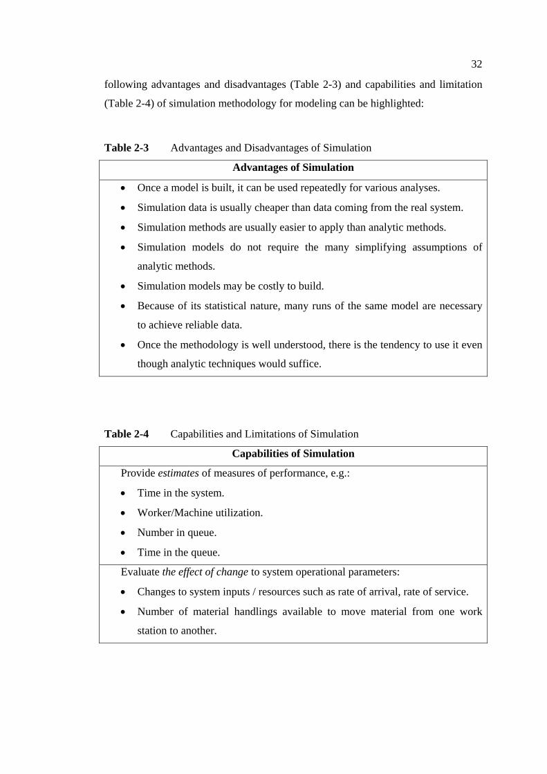
following advantages and disadvantages (Table 2-3) and capabilities and limitation

(Table 2-4) of simulation methodology for modeling can be highlighted:

Table 2-3 Advantages and Disadvantages of Simulation

Advantages of Simulation

• Once a model is built, it can be used repeatedly for various analyses.

• Simulation data is usually cheaper than data coming from the real system.

• Simulation methods are usually easier to apply than analytic methods.

• Simulation models do not require the many simplifying assumptions of

analytic methods.

• Simulation models may be costly to build.

• Because of its statistical nature, many runs of the same model are necessary

to achieve reliable data.

• Once the methodology is well understood, there is the tendency to use it even

though analytic techniques would suffice.

Table 2-4 Capabilities and Limitations of Simulation

Capabilities of Simulation

Provide estimates of measures of performance, e.g.:

• Time in the system.

• Worker/Machine utilization.

• Number in queue.

• Time in the queue.

Evaluate the effect of change to system operational parameters:

• Changes to system inputs / resources such as rate of arrival, rate of service.

• Number of material handlings available to move material from one work

station to another.

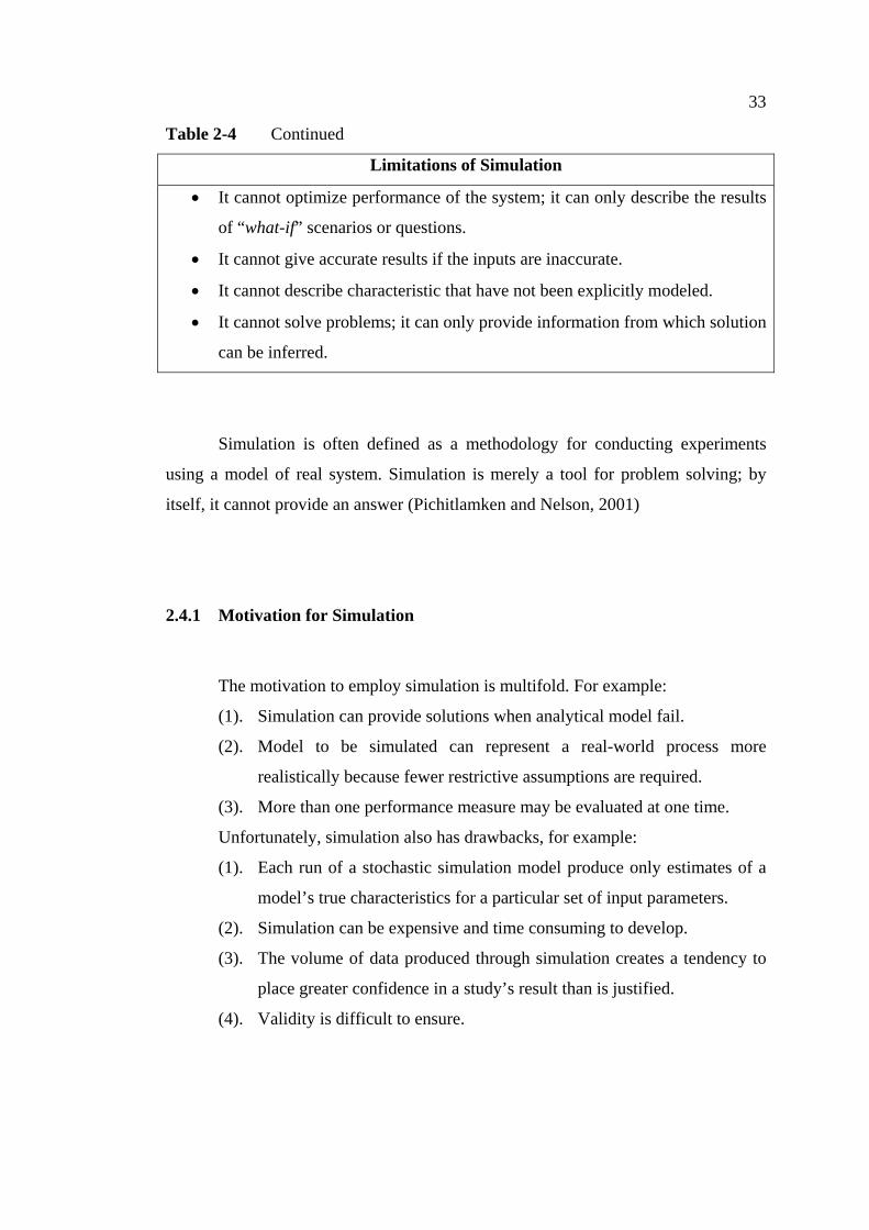
33

Table 2-4 Continued

Limitations of Simulation

• It cannot optimize performance of the system; it can only describe the results

of “what-if” scenarios or questions.

• It cannot give accurate results if the inputs are inaccurate.

• It cannot describe characteristic that have not been explicitly modeled.

• It cannot solve problems; it can only provide information from which solution

can be inferred.

Simulation is often defined as a methodology for conducting experiments

using a model of real system. Simulation is merely a tool for problem solving; by

itself, it cannot provide an answer (Pichitlamken and Nelson, 2001)

2.4.1 Motivation for Simulation

The motivation to employ simulation is multifold. For example:

(1). Simulation can provide solutions when analytical model fail.

(2). Model to be simulated can represent a real-world process more

realistically because fewer restrictive assumptions are required.

(3). More than one performance measure may be evaluated at one time.

Unfortunately, simulation also has drawbacks, for example:

(1). Each run of a stochastic simulation model produce only estimates of a

model’s true characteristics for a particular set of input parameters.

(2). Simulation can be expensive and time consuming to develop.

(3). The volume of data produced through simulation creates a tendency to

place greater confidence in a study’s result than is justified.

(4). Validity is difficult to ensure.

34

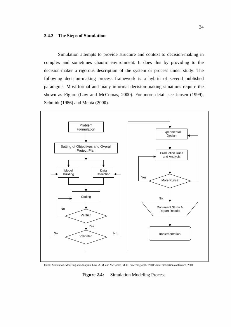
2.4.2 The Steps of Simulation

Simulation attempts to provide structure and context to decision-making in

complex and sometimes chaotic environment. It does this by providing to the

decision-maker a rigorous description of the system or process under study. The

following decision-making process framework is a hybrid of several published

paradigms. Most formal and many informal decision-making situations require the

shown as Figure (Law and McComas, 2000). For more detail see Jensen (1999),

Schmidt (1986) and Mehta (2000).

Form: Simulation, Modeling and Analysis, Law, A. M. and McComas, M. G. Proceding of the 2000 winter simulation conference, 2000.

Figure 2.4: Simulation Modeling Process

Problem Formulation

Setting of Objectives and Overall Project Plan

Model Building

Data Collection

Coding

Experimental Design

Production Runs and Analysis

Verified

Document Study & Report Results

Implementation

Validated

More Runs?

No

No No

No

Yes

Yes

35

1. Need Recognition.

First, one observes a phenomenon to investigate or question to research. At

this stage, questions are often ill-defined and may exist as little more than a hunch

that something is wrong or needs adjustment.

2. Problem Formulation

After a bit of though and some preliminary investigation a specific question

or set of question emerge. This step often includes the identification of alternatives

and the choice of a criterion by which to make a decision.

3. Model Construction

Third, one decides on a context in which to ask formulated question. This

may include constructing a mental model, building a physical model, conceptualizing

an analog, or developing a mathematical representation of the problem. In this class

we shall spend a great deal of time constructing mathematical models but it is vital to

note that this activity is but one in the framework. Here, we shall concentrate on

computer simulation.

4. Data Collection

Data collection describes the mean to generate data input for modeling. There

are at least as many ways to generate data as there are modeling techniques. A

difficult question that must be answered pertains to the amount of data to be

36

collected and the level of data aggregation required. Sets of simplifying assumptions

are usually required.

5. Model Solution

A significant advantage of mathematical models is that once they constructed

(and the required data is generated) solution is trivial. In most solution, solution

procedures can be routinized and then automated. This is often not the case of mental

and physical models.

6. Model Reliability and Validity

Once a model is built, a check for reliability is made to insure that multiple

solution of the same model yield the same result. After reliability is assured, one may

compare the solution with an expectation of reality. If the model behaves as expected

then one has some level of confirmation that the model is ‘valid”. If not, then a return

to model construction may be warranted. In same case, model building leads one to

ensure their view of reality.

7. Interpretation of Result, Implications and Sensitivity Analysis.

A reliable and valid model is useless unless one can interpret its solution and

apply that solution to a given situation. Additionally, one may wish to describe the

consequence of slight departures from assumption or model parameters. Any

“sensitive” aspect of our model will cause significant differences in solution. These

aspects must be closely monitored and controlled.

37

2.4.3 Scheduling Through Simulation

Each job may have one or more operations remaining before the completion

of the order. The sequence of work centers ("machines") through which a job flows

constitutes the job's routing. The routings for various jobs will, in general, vary

widely. For example, one job may go first to a lathe, then a milling machine, and

finally a drill press, while another job may go to a bender and then to a punch press.

The operation required at each machine normally includes a machine setup and

actual run time. A given job may involve work on a single piece or on multiple

pieces that are processed in a single batch. The shop can be scheduled by means of a

simulator. Beginning with the existing state of the shop, the flow of work through the

shop can be simulated. Upon completion of all jobs in simulated time, the simulated

results can be analyzed. Results may be measured in such terms as the total hours of

job tardiness and the total time jobs are in the shop (flow time). If the results appear

satisfactory, the sequence of events in simulated time can be taken as the scheduled

events. If results are not satisfactory, the shop can be simulated again using different

machine capacities or different decision rules. This can continue until a satisfactory

schedule is found, or until it is concluded that further search is unwarranted.

The basic simulation cycle is triggered with the completion of an operation. It

consists of the following steps:

(1). Determine which machine next finishes an operation.

(2). Assign to the now free machine the highest priority job in the queue.

(3). Move the job that just completed an operation to its next machine, or, if

all operations have been completed, remove the job from the shop.

2.5 Design of Simulation Experimentation

Simulation-based approaches are derivatives of dispatching rule-based

approaches. In a simulation-based scenario, one or more dispatching rules may be

used to make a decision when a resources becomes available. Simulation-based

38

approaches are restricted mostly to a forward scheduling capability (i.e., where a

schedule is constructed by starting from a reference time and then advances the

simulation clock as jobs are scheduled on resources). Simulation models are able to

represent the detail of scheduling situations, and simulation-based approaches are

useful in communicating the specific detail to various levels of personnel because of

visual aids (e.g., animation) offered by simulation.

From the simulation view point, a job is considered as a queuing network

where an order may require several different operations by different machines and

may have to wait in several different queues. If job arrive at the shop randomly over

time, the job shop is referred to as a dynamic job shop. This chapter present a review

of basic factors incorporated into simulation models of dynamic job shops and

therefore provide a basic understanding of a job shop simulation model for

scheduling analysis. The second goal of this chapter is to provide a basic

understanding of scheduling rules and their performance in simulated job shop.

The most likely components of job shop simulation model are as follows:

1. Order arrivals

2. Processing and setup times

3. Machines

4. Job routings

5. Shop load factor

6. Due dates

7. Priority rules

2.5.1 Order Arrivals

The arrival of orders is modeled in one of the following ways:

1. Instantaneous release of order into the shop. In this approaches the next order

arrival times is defined at the time of each order arrival. The time between

these arrivals is defined as a randomly generated variable.

2. Periodical release of all available orders at the beginning of the schedule

period (day, week, etc.). This can be modeled in two ways:

39

a. All the arriving orders as defined above accumulate at an order

entry point. All of these orders are released into the shop at

predefined points in time.

b. At each order release time, a number defined as random

variable of orders is generated.

3. Order pooling. This is similar to the above, except that a subset of the

available orders is released into the shop at the beginning of each scheduling

period. The selection of orders to be released into the shop may be based on

the shop load and order characteristics.

The first approach is used in most models. The most popular arrival pattern is

that of the Poisson process (i.e., the Poisson arrival rate or exponentially distributed

inter-arrival times). If the time between arrivals is exponentially distributed, the rate

(i.e., the number of arrivals per unit time) has a Poisson distribution. Therefore the

Poisson-distributed arrival rate (in orders per unit time) is translated into interarrival

time of the corresponding exponential distribution. However, when periodic release

or order pooling is utilized, the Poisson may directly represent the number of orders

arriving in an hour, day, and so on. The Erlang distribution is the sum of exponential

distributions and is also used to model order arrivals. Other distributions for the

interarrival time or arrival rates are uniform, geometric, binomial, and empirical

(actual shop data) distributions. Constant interarrival times also used in investigating

shop performance or the sensitivity of shop performance and the priority rules to

some order and shop parameter.

The prevalence of the Poisson process is probably a result of its widespread use

in queuing theory and its observed validity in some practical situations (e.g., number

of calls arriving at a switchboard). The observed distribution of arrivals in actual

shops, however, shows a wide variety in the arrival rate, and the Poisson distribution

is not sufficient to explain or fit all the distributions observed. If the number of

sources generating orders decreases, applicability of the Poisson assumption

diminishes. For example, if orders to the shop are generated by distribution center

based on minimum order levels, the consolidated order patterns may be erratic, even

if the customer order pattern may be a Poisson process.

40

Several different studies report that the arrival pattern is not important in

evaluating the relative effectiveness of priority rules, although shop performance can

be affected by the arrival pattern. Studies investigating periodic release and order

pooling indicate similar result. In general, shop performance decrease with the

increasing variance of the interarrival time distribution. Under periodic release, the

following conclusion where obtained in various simulation studies:

1. The mean and variance of the inventory level are higher with an increase

in the release period ( Panwalkar, et. al. 1976).

2. Utilization is higher than average at the beginning of a scheduling period

but is lower at the end ( Panwalkar, et. al. 1976).

3. Fewer jobs are tardy for periodic release; however, the job that are tardy

have longer periods of tardiness (Ulgen, O., 1979).

4. Due date performance is improved when period release is combined with a

scheduling rule (Holloway and Nelson, 1974).

5. Job pooling (i.e., releasing a subset of orders at predefined intervals) is

more restrictive and usually causes a decrease in shop performance (Ulgen,

1979) However, if the subset is selected to be balance the machine

workloads, job pooling has a positive effect on shop and workload balance

measures but has no significant effect or worse results on variance of

lateness distribution and average tardiness (Irastorza and Deane, 1974).

2.5.2 Processing and Setup Times

In most job shop simulation models, the processing times are determined

when an order arrives at the shop. Two approaches at this point:

1. Generate the actual processing times from a specified distribution; the

processing times are random variables from a distribution such as the

exponential distribution.

2. Generate the estimate processing times; the estimated times are the

information available for scheduling purposes. When an order is placed

on a machine, a random variable called a work rate factor is generated

and is multiplied by the estimated time to give the actual time required.

41

The most common distributions are exponential and uniform for the

estimated times and triangular, normal, or uniform for the work rate

factor. This approach simulates the fact that in most cases the scheduler’s

knowledge or the processing times is not accurate and the process times

fluctuate during day-of-day operations due to uncontrollable factors.

The specified families of processing time distributions are associated

parameter affect shop performance. More important, some priority rules, such as

SPT, are more sensitive to processing time distributions than are others. In general,

as the variability of the order processing time decrease, performance of the non-due-

date scheduling rule improves.

The setup times are included in the processing times in most models. In some

models dependent setup times are used, the distribution of these times must be

selected along with the parameter values. As the variance increases, the desirability

for minimizing the setup times increases. The relative values of mean setup time and

the mean processing time are also important considerations. When the mean setup

time is large with respect to the mean processing time, there are more benefits

obtainable from the scheduling rules that minimize the setup times.

In recent models, due to the increased capability and easy of modeling, a

sequence-dependent setup time has been used. The presence of sequence-dependent

setups changes both shop performance and the performance of the priority rules.

Priority rules, which take setup times into consideration, are more successful than the

others when the setup times are strongly sequence dependent (e.g., changing from J1

to J2 takes 10 minutes but changing from J3 to J2 takes 120 minutes).

2.5.3 Number of Machines

The number of machines used in simulation models varies greatly. In

hypothetical models designed to evaluate the performance of scheduling rules, the

number of machines range from 4 to 15. There seem to be a consensus that a four-

machines shop model is large enough so that the result can be extrapolated to the

42

more complex shops. Some comparative studies have investigated the effect of shop

size on the relative effectiveness of the priority rules and conclude with similar

result: that neither the size nor the configuration of the shop changes the relative

effectiveness of the priority rules.

2.5.4 Job Routing

Job routing determines the required sequence of operation so as to predict the

traveling pattern of orders among the machines. Diversity of order types is imported

to the models via a routing matrix, which defines the transition probabilities of orders

from one machine to next. The extreme case are the pure flow shop, where there is

only one routing, and the pure job shop, where the transient probabilities between the

machines are equal for subsequent operations. Pure job shop models are the most

common types of models in simulation studies. This is partly because of the easier

load control over the shop in pure job shop models.

Often in real system, some or all orders may have alternative routings such

that an operation may be performed on any one of number of machines. Two

approaches are possible when alternative routing exist:

1. Place the order in all feasible operation queues. Perform the

operation on the first available machine; remove the order from the

other queues when the order is assigned to a machine.

2. Assign the order to an idle machine that is capable of performing a

feasible operation; if there is no such idle machine, place the order

in a queue according to some queue selection rule (e.g., shortest

queue length, least work in queue, etc.).

Alternative routing has a significant impact on shop performance and on the

relative effectiveness of the priority rules; It provides better performance and reduces

the difference between the priority rules.

43

2.5.5 Machine and Shop Utilization

The combined effect of order arrival distribution, job routing, and processing

times determine machine utilization. From the standpoint of job shop simulation,

machine utilization is important because it affect queue lengths. If the average queue

length is too small, the scheduling rules used in the model may not be forced to make

discriminating order selections. When this situation occurs, it is difficult or

impossible to evaluate the effectiveness of the scheduling rule. Adverse effects also

result from machine utilization that is too high. If utilization is near 1.00, transient

conditions may extend over long periods and require excessive CPU time in order to

obtain a steady state that permits data to be collected for comparison purposes.

Machine utilization commonly found in the literature ranges from 0.85 to 0.95.

Utilizations in this range usually cause queues to reach a length that permits

scheduling rules to select an order from several in the queue but does not lead to very

long queues.

Sequence-dependent setup times may require careful consideration due to

their effect on machine utilization and hence queue lengths. When some scheduling

rules yield significantly different average setup times than some other rules, the

model results may produce small queues. On the other hand, if another scheduling

rule does not consider setup times, the combined setup plus the processing times may

cause a saturation of the shop and thus produce an undesirable effect.

2.5.6 Due Date

Several different studies indicates that shop performance and the relative

effectiveness of priority rules are affected by due date assignment methods as well by

the tightness of due dates. The following considerations related to due date

assignment:

1. Through policy (fixed) parameters, each order is assigned a due

date when it arrives at the shop. The due date assignment method

may or may not use current shop information:

44

a. Static due date assignment rules consider only order data such

as the arrival time, routing, and operation processing times of

an order. Hence the order allowance time is a fixed amount for

a given order of data and does not depend on the shop status

when the order arrives.

b. Dynamic due date assignment methods employ order and shop

data. In addition to the arrival times, operation times, and

routing, other factors in due date determination may include

the current shop load and the average waiting time of the

orders.

2. Due date assignment and order sequencing decision may be

considered together and simultaneously as two dependent factors in

the planning process. This leads to a new problem that requires

determination of both the optimal set of due date and schedule for a

given situation involving the shop status and order parameters.

2.5.7 Priority Rules

In the scheduling literature, a variety of terms, such as scheduling rule,

priority rule, dispatching rule, or heuristic, refer to the rule that select an order from

the order waiting in a queue to be processed next by the machine. However, a

distinction is possible for clarification purpose: Usually, a priority rule is defined as a

method of assigning a scalar value to each order in a queue fro scheduling purpose.

A dispatching rule is defined similarly but implies that after the priorities are

assigned, the job with the most priority will be dispatched to an available machine. A

heuristic implies that more complex mathematical rules are used in determining the

priorities. Finally, a scheduling rule may employ one or more priority rules and/or

more complex mathematical or heuristic concepts in determining the next order to be

45

processed. In practice, the basic term priority or dispatching rule is used for all of the

above.

Priority rules may be classified according to their time dependency (static

versus dynamic rules), the type of data they use (local versus global rules), or both. A

static rule determines only one priority value for each operation of an order during its

existence in the shop. A dynamic priority value, in contrast, change over time, to

assign the right order (i.e., the order that has the highest actual priority) to an

available machine. The priority values of order must be updated before each decision

is made. Hence more calculation is involved in dynamic rules. Adam and Surkis

(1980). Priority update interval and anomalies in dynamic ratio type job shop

scheduling rules, investigated the effect of updating policy and of updating the

intervals on computational requirements and the effectiveness of priority rules. They

concluded that due date performance is sensitive to the updating policy and to the

updating intervals especially at high utilization (i.e., 92 to 96%).

Panwalkar and Iskander (2001) describe and categorized 113 priority rules.

The functional categorization is given below.

1. (a). Simple priority rules are based on order and/or shop data such as

processing times, due date number of operations, cost(values),

setup times, arrival times, and slack.

(b). The combinations of simple priority rules are the applications of

two or more priority rules with the selection of which rule to use

at a specific time being a function of the queue and order

characteristics.

(c). Weighted priority rules involve the application of rules in 1(a)

and/or 1(b) combined with different weights.

2. Heuristic involve more complex considerations, such as the solving of

static problem at the beginning of each scheduling period, look-ahead,

and so on.

3. Other rules.

The body of job shop simulation research established the validity of the basic

assumption that given all the other shop parameters are the same, shop performance

46

is strongly affected by the priority rules being used. However, there is no clear

winner claimed for all the performance measures.

2.6 Simulation and Its Application on Scheduling

Mathematical models are a formalism whereby we can summarize our

understanding of the physical world and utilize this knowledge in calculations of

engineering interest. An important feature of any model is that it accurately reflects

only those phenomena relevant to the current activity. On the one hand, accuracy is

crucial to the utility of the results, and, on the other, relevance avoids unnecessary

computation in achieving results and avoids obscuring important conclusions in the

details.

Simulation is defined as the imitation of the operation of a real world process

or system over time (Banks, 1998). Simulation is a necessary problem solving

methodology for the solution of many real world problems. Simulation is used to

describe and analyze the behavior of a system, as what-if question about the real

system, and aid in the design of real systems. Existing system and conceptual system

can be modeled with simulation. In other word (Shannon, 1975): simulation is an

experimental techniques and applied methodology which seeks (i) to describe the

behavior of system, (ii) To construct theories or hypotheses that account for the

observed behavior, and (iii) To use these theories to predict future behavior or the

effect produced by changes in the operational input set.

Many researches has used simulation methodology to solved scheduling

problems (Yang and Wang, 2001, Cheng, Gen, and Tsujimura, 1996, Fonseca and

Navaresse, 2002, Maturana, et. al. , 1997, Kacem, Hammadi, and Borne, 2002, Ying,

1996, and Sadeh and Fox, 1996.) Karatza, 2000, Chong and Sivakumar, 2003. In

Term of Dynamic Simulation (Maturana, et al., 1997, Kacem, Hammadi and Borne,

2002, Ying, 1996, and Sadeh and Fox, 1996.). or Stochastic Simulation Yang and

Wang, 2001, Fonseca and Navaresse, 2002.

47

Simulation modeling is a highly flexible technique because its models do not

require the many simplifying assumption needed by most analytical techniques.

Furthermore, simulation tends to be easier to apply than analytic methods. In

addition, simulation data is usually less costly than data collected using a real system.

However, constructing simulation models may be costly, particularly because they

need to be thoroughly verified and validated. Additionally, the cost of the experiment

may be increase nature of simulation requires time increases. The statistical nature of

simulation requires that many runs of the same model be done to achieve reliable and

accurate results. Although its flexibility, simulation modeling traditionally is not an

optimization techniques

Simulation system has become a powerful decision making instrument for

scheduling. It requires a few simplifying assumptions, captures many of the true

characteristics of the real model, and provides good insights about the interactions

and relationships between qualitative and quantitative variables. This section

describe recent research on simulation in scheduling by many authors.

Chong and Sivakumar, (2003) presented A simulation-based real-time

scheduling mechanism for dynamic discrete manufacturing. The authors use mean

flow time performance for different scheduling approaches, subjects to disturbances

such as machine breakdowns. Discrete event simulation is used on-line to evaluate

the selected approaches and the corresponding schedules to determine the best

solution. The authors conclude that discrete event simulation has been an essential

tool for detailed scheduling under a highly dynamic and unpredictable manufacturing

system.

Cave, Nahavandi, and Kouzani (2002) introduce simulated annealing for

simulation optimization of a real scheduling problem in industry. The authors

showed that when using this method, high quality schedules can be produced within

reasonable time constraints, but still not less computational yet.

Karatza (2000) Studied scheduling simulation model to address performance

issues associated with scheduling. Three policies which combine processor and I/O

scheduling are used to schedule parallel jobs for a variety of workloads. Simulated

results reveal that all scheduling methods have merit, but one method significantly

48

improves the overall performance and also provides a guarantee for fairness in

individual job execution.

2.5 ANN for Solving Scheduling Problems

An artificial neural network (ANNs) is one of the AI techniques that have

gained an important role in solving problems with extreme difficult or unknown

analytical solutions (Lawrence, 1994). An ANN consists of an interconnected web of

special units, called neurons, with associated connection weights that, after receiving

a proper training, are capable of achieving a desired response to new inputs. Its

ability of learning from examples makes ANN an extremely powerful programming

tool when domain rules are not completely certain or when some amount of

inaccuracy or conflicting data exist (Medsker, 1994). An ANN is used to learn a

functional relationship between a set of jobs and the corresponding to the set of

machine in the shop that optimize the stated performance criterion. The ‘trained’

neural network is then able to apply the learnt relationship to new problems.

There are some approaches developed based on artificial intelligence

techniques such as neural networks, expert systems, fuzzy logic and genetic

algorithms. There are some approaches developed based on artificial intelligence

techniques such as neural networks, expert systems, fuzzy logic and genetic

algorithms. Among them, Bilkay et al. (2004) proposed algorithm for flexible

manufacturing system by using fuzzy logic. Yu and Ling (2001) involved neural

network and genetic algorithm to solve the expanded job-shop scheduling problem.

Genetic algorithms (GAs) are also used independently for JSS by some researches,

among them Brizuela and Sannomiya (1999), Madureira and Ramos, (2001), Zhou

et al. (2001). Watanabe, 2003 using ANN for solves Job shop scheduling.

Sabuncuoglu and Gurgun (1996) propose a new neural network approach to

solve the single machine mean tardiness scheduling problem and the minimum

makespan job shop scheduling problem. The proposed network combines the

characteristics of neural networks and algorithmic approaches. The performance of

49

the network is compared with the existing scheduling algorithms under various

experimental conditions. A comprehensive bibliography is also provided in the

paper.

El-Bouri et al. (2000) presented an approach for single machine job

sequencing problems that is based on artificial neural networks. A problem is

classified first by one type of neural network into one of a number of categories. The

categorization is based on the problems characteristics. Then another neural network,

which is specialized for a particular category, applies a previously learning

relationship to produce a job sequence that aims to better satisfy the given objective.

The learning is acquired in these networks after a training process in which the

network is exposed repeatedly to a set of example problems and their solutions. The

trained network thereby learns predominant relationships between given problems,

and the output sequences that optimally meet the desired objective. The advantage of

such an approach is that it allows what amounts to a “customized” heuristic to be

established for problem subsets and various objectives without having to deduce an

algorithm in advance. The methodology and its implementation is described for

several of the more common sequencing objectives, as well as for a hypothetical

objective that minimizes a cost function exhibiting a limited exponential behavior.

Lee and Shaw (2000) consider the classic problem of sequencing a set of jobs

that arrive in different combinations over time in a manufacturing flow-shop. They

focus on the development of a two-level neural network that incrementally learns

sequencing knowledge. Based on the knowledge gained from learning using a set of

training exemplars, the neural network makes real time sequencing decisions for a set

of jobs that arrive in different job combinations. In addition to explain the details

regarding the workings of the neural network, they also evaluate its performance for

flow-shop sequencing problems. The practical benefit of the neural-net approach is

that the neural network incrementally learns the sequencing knowledge and can

apply the knowledge for sequencing a set of jobs on a real time basis. They also

show that the neural network can be used to develop hybrid genetic algorithms. The

experimental results demonstrate that (1) the neural-net approach produces

consistently superior solution quality (i.e., makespan) with significantly less

computational time than the traditional heuristic approaches; (2) when compared to

50

genetic algorithms the neural-net approach's performances are within 3.4% of those

of genetic algorithms, but using only less than 0.2% of the computational time

needed by genetic algorithms; and (3) the neural-net approach further improves

solution quality and computational time by combining it with genetic algorithms.

Yang and Wang (2001), presented a new adaptive neural network and

heuristics hybrid approach for job-shop scheduling is presented. The neural network

has the property of adapting its connection weights and biases of neural units while

solving the feasible solution. Two heuristics are presented, which can be combined

with the neural network. One heuristic is used to accelerate the solving process of the

neural network and guarantee its convergence; the other heuristic is used to obtain

non-delay schedules from the feasible solutions gained by the neural network.

Computer simulations have shown that the proposed hybrid approach is of high

speed and efficiency. The strategy for solving practical job-shop scheduling

problems is provided.

Yu and Liang (2001), presented a hybrid approach involving neural network

and genetic algorithm (GA) to solve the expanded job-shop scheduling problem

(EJSSP). The GA is used for optimization of sequence and a neural network (NN) is

used for optimizing of operation start times with a fixed sequence. The authors

reported that the approach has been shown powerful for competes expanded job-shop

scheduling problem.

2.5 Summary of Chapter 2

This chapter has provided a broad and specific review on issues related to

scheduling. In particular, scheduling classification and scheduling rules were

reviewed to provide general background information on the field of study. It also

provides specific reviews on job shop scheduling and dynamic scheduling since these

are the focus problem in this study. This reviews also covered previous studies

conducted by various researchers on dynamic scheduling. Background on the

simulation techniques and its application in scheduling studies were also reviewed.

51

In addressing the dynamic job shop scheduling problem, close-form mathematical

and optimization procedures would have difficulty in capturing the complexities and

not capable to provide solution in a reasonable amount of time. Artificial neural

network has been identified as a promising information processing tools in many

fields of studies. Its applications in solving scheduling problems were also reviewed

in this report.

CHAPTER 3

RESEARCH METHODOLOGY

This chapter describes the methodology adopted in this research. It begins

with description of the traditional and proposed frameworks for producing

production schedules. Then it describes the operational framework, research

questions and development phases.

3.1 Traditional and Proposed Framework

Since the job shop scheduling problem is a well-known NP hard problem, a

realistic size of the problem can not be solved by searching and evaluating all the

alternative solutions. Generally, there are no optimization algorithms which can

solve a NP hard problem in a polynomial time. However, such problem may be

solved using heuristics algorithms with approximated optimal solution. There are

many literatures which report various heuristic methods to solve such problems. One

alternative technique is through simulation. This approach has been extensively

applied in many application areas including the job shop-scheduling problem. The

main problem in applying this approach is that the user needs to re-run the simulation

whenever there are changes in the system. This traditional approach is time

consuming and not practical for a dynamically changing manufacturing environment.

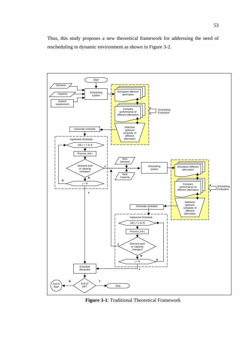
53

Thus, this study proposes a new theoretical framework for addressing the need of

rescheduling in dynamic environment as shown in Figure 3-2.

Figure 3-1: Traditional Theoretical Framework

Y

New Demand

New Capacity

Generate schedule

Implement Schedule

Job j = 1 to N

Process Job j

Demand and/ or capacity changes?

j = N

N N

Schedule discarded

Y

Stop Got to Start

N Y End of job?

Scheduling system

Generate schedule

Start

Scheduling system

Demand

Capacity

System requirement

Implement Schedule

Job j = 1 to N

Process Job j

Demand and/ or capacity changes?

j = N

N N

SchedulingEvaluation

Simulation different alternation

Compare performance of

different alternation

Selectionoptimum

schedule of different

alternation

SchedulingEvaluation

Simulation different alternation

Compare performance of

different alternation

Selection optimum

schedule of different

alternation

Y

Y

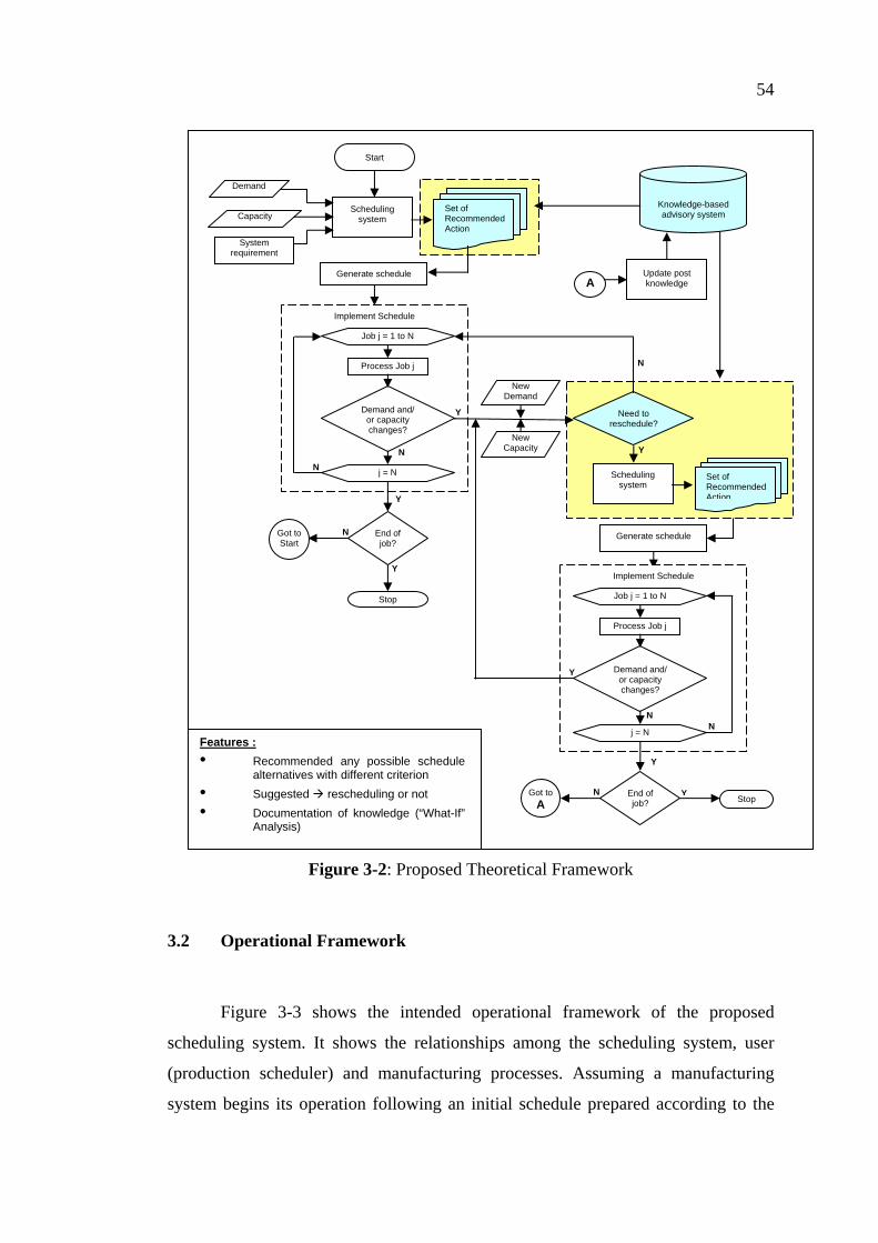
54

Figure 3-2: Proposed Theoretical Framework

3.2 Operational Framework

Figure 3-3 shows the intended operational framework of the proposed

scheduling system. It shows the relationships among the scheduling system, user

(production scheduler) and manufacturing processes. Assuming a manufacturing

system begins its operation following an initial schedule prepared according to the

Features : • Recommended any possible schedule

alternatives with different criterion • Suggested rescheduling or not • Documentation of knowledge (“What-If”

Analysis)

New Demand

New Capacity

Generate schedule

Need to

reschedule?

Scheduling system

Set of Recommended Action

Y

N

Stop

Got to Start

N

Y

End of job?

Y Stop Got to

A N

Y

End of job?

Implement Schedule

Job j = 1 to N

Process Job j

Demand and/ or capacity changes?

j = N

N

Y

Y

Implement Schedule

Job j = 1 to N

Process Job j

Demand and/ or capacity changes?

j = N

N N

Generate schedule

Start

Scheduling

system Set of Recommended Action

Demand

Capacity

System requirement

Y

N

Update post knowledge

Knowledge-based advisory system

A

55

present job shop condition. However, when changes emerge in demand or capacity,

the production scheduler has to immediately update the system with new

information. Then, the scheduling system would instantaneously generate the revised

schedules without a need to evaluate or simulate the new manufacturing scenarios.

Figure 3-3: Operational Framework

3.3 Research Questions

The literature reviews as discussed in Chapter 2 reveal some research

questions regarding potential and applicability of neural network technique in

development of a scheduling system for a dynamic job shop. Among the unanswered

question are:

• Job details • Process detail • Scheduling

strategies • etc.

Manufacturing Process

Demand Status

Capacity Status

Sets of recommended action

• Performance measures

• Machine utilization• etc.

Selected Schedule

Production Scheduler

System Requirement

Scheduling System

56

- Can ANN supplement or replace the existing method in the process of

generating schedules?

- Can ANN supplement or replace the existing method for selecting the best

schedule/decision for a given set of conditions for dynamic job shop

scheduling?

This research also seeks to address the above questions.

3.4 Development Phases

The development phases used in this study comprises two phases as shown in

Figure 3-4:

Phase 1: Simulation studies of various scheduling scenarios.

Phase 2: Design and development of a dynamic scheduling system by using

artificial neural network (ANN).

Figure 3-4: Development Phases

Data collection

Simulation

Design and Development of ANN-based Scheduling

System

Training of ANN

Schedule Perf.

Trained schedule scenarios

Implementation

Phase 1. Data collection and data generated

Phase 2. Model Design and development

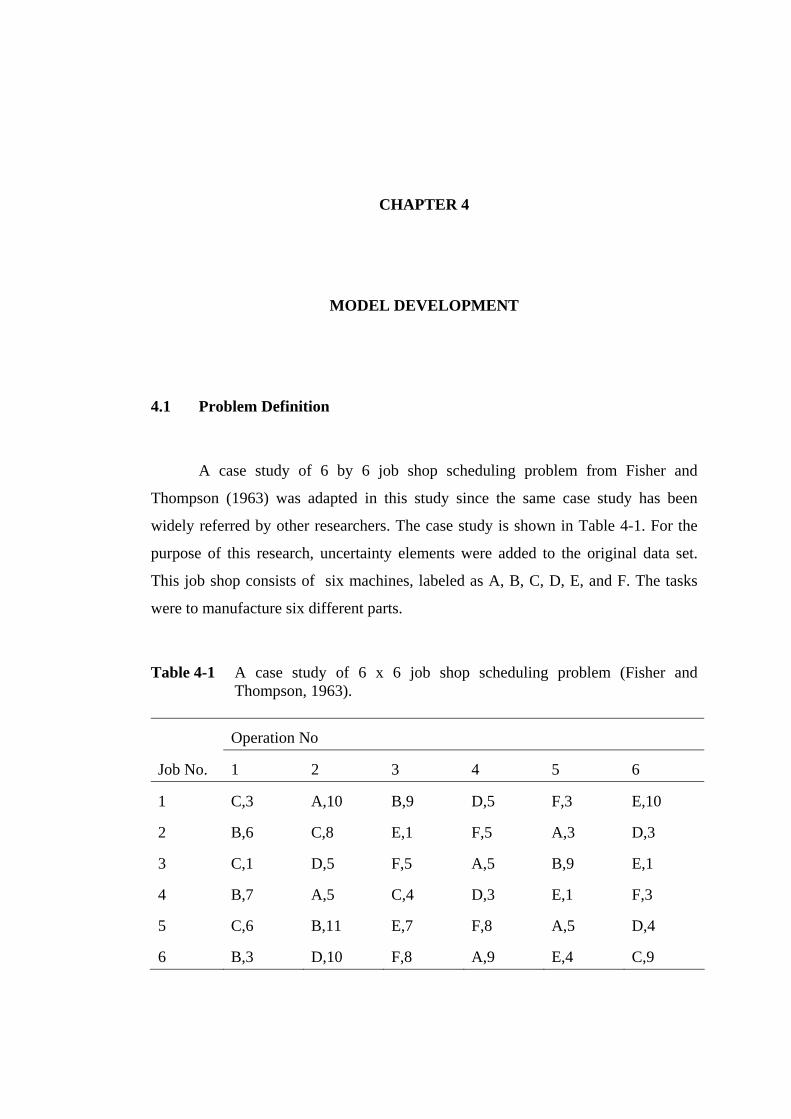
CHAPTER 4

MODEL DEVELOPMENT

4.1 Problem Definition

A case study of 6 by 6 job shop scheduling problem from Fisher and

Thompson (1963) was adapted in this study since the same case study has been

widely referred by other researchers. The case study is shown in Table 4-1. For the

purpose of this research, uncertainty elements were added to the original data set.

This job shop consists of six machines, labeled as A, B, C, D, E, and F. The tasks

were to manufacture six different parts.

Table 4-1 A case study of 6 x 6 job shop scheduling problem (Fisher and Thompson, 1963).

Operation No

Job No. 1 2 3 4 5 6

1 C,3 A,10 B,9 D,5 F,3 E,10

2 B,6 C,8 E,1 F,5 A,3 D,3

3 C,1 D,5 F,5 A,5 B,9 E,1

4 B,7 A,5 C,4 D,3 E,1 F,3

5 C,6 B,11 E,7 F,8 A,5 D,4

6 B,3 D,10 F,8 A,9 E,4 C,9

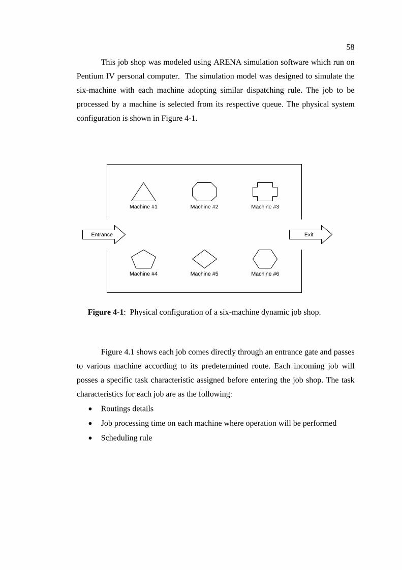
58

This job shop was modeled using ARENA simulation software which run on

Pentium IV personal computer. The simulation model was designed to simulate the

six-machine with each machine adopting similar dispatching rule. The job to be

processed by a machine is selected from its respective queue. The physical system

configuration is shown in Figure 4-1.

Figure 4.1 shows each job comes directly through an entrance gate and passes

to various machine according to its predetermined route. Each incoming job will

posses a specific task characteristic assigned before entering the job shop. The task

characteristics for each job are as the following:

• Routings details

• Job processing time on each machine where operation will be performed

• Scheduling rule

Machine #1 Machine #2 Machine #3

Machine #4 Machine #5 Machine #6

Entrance Exit

Figure 4-1: Physical configuration of a six-machine dynamic job shop.

59

4-2 Simulation Model

As noted earlier, a computer simulation model to represent the job shop

system was designed using ARENA. The performances of various job shop

conditions when using scheduling rules, namely, first-in-first-out (FIFO), earliest-

due-date (EDD), and shortest processing time (SPT) were evaluated.

The job shop used in this study consists of 6 unique work centers. The jobs

were planned to arrive continuously with inter-arrival times generated from an

empirical discrete distribution. The mean value chosen was chosen to create a certain

expected shop utilization rate. Each job underwent 6 operations which were drawn

from a normal distribution with means extracted from the original data (Fisher and

Thompson,1963). The schedule adopted a pure job shop routing whereby when a job

left a work center, it was equally likely to go to each of the other work centers. Work

center processing times were drawn from a normal distribution with means extracted

from Fisher and Thompson (1963). Other assumptions adopted in the development of

the model are :

• the resources were available continuously

• preemption of a job was not allowed

• set-up times were included in the processing times

• transportation times were excluded, and

• processing times of the jobs were known after their arrivals at the shop.

4.2.1 Steady-state Condition of the Shop (Warm up period)

In order to ascertain when the system has achieved a steady state, the shop

parameters, such as the machine utilization level and mean flow-time of jobs need to

be observed. It was found that the simulated system reached a steady state after the

arrival of about 500 time units.

60

4.2.2 Run Length and Number of Replications

Job arrivals were generated using an exponential distribution. Three machine

utilization levels, namely, “low”, “medium”, and “high” were studied. Thus, in all,

for one type of process time distribution, one due date setting and three different

utilization levels would resulted in a total of three experimental sets for every

dispatching rule. Hence, for the three scheduling rules (FCFS, EDD and SPT), a total

of nine simulation experiments were conducted. Each simulation experiment was

replicated in twenty different runs. In each run, the job shop was continuously loaded

with job orders that were numbered on arrival.

4.3 Artificial Neural Network Model

The construction of the artificial neural network (ANN) model involves a

learning process. Figure 4-2 illustrates the neural network model developed for this

research. The network was developed using a multilayer perceptron (MLP)

architecture and the learning process was based on back-propagation algorithm. The

datasets for training and testing were stored in a text file. The ANN learning involves

computation of the predicted output against the target output. Adjustment of the

weight was made to minimize the mean absolute error (MAE) as shown in Figure 4-

3.

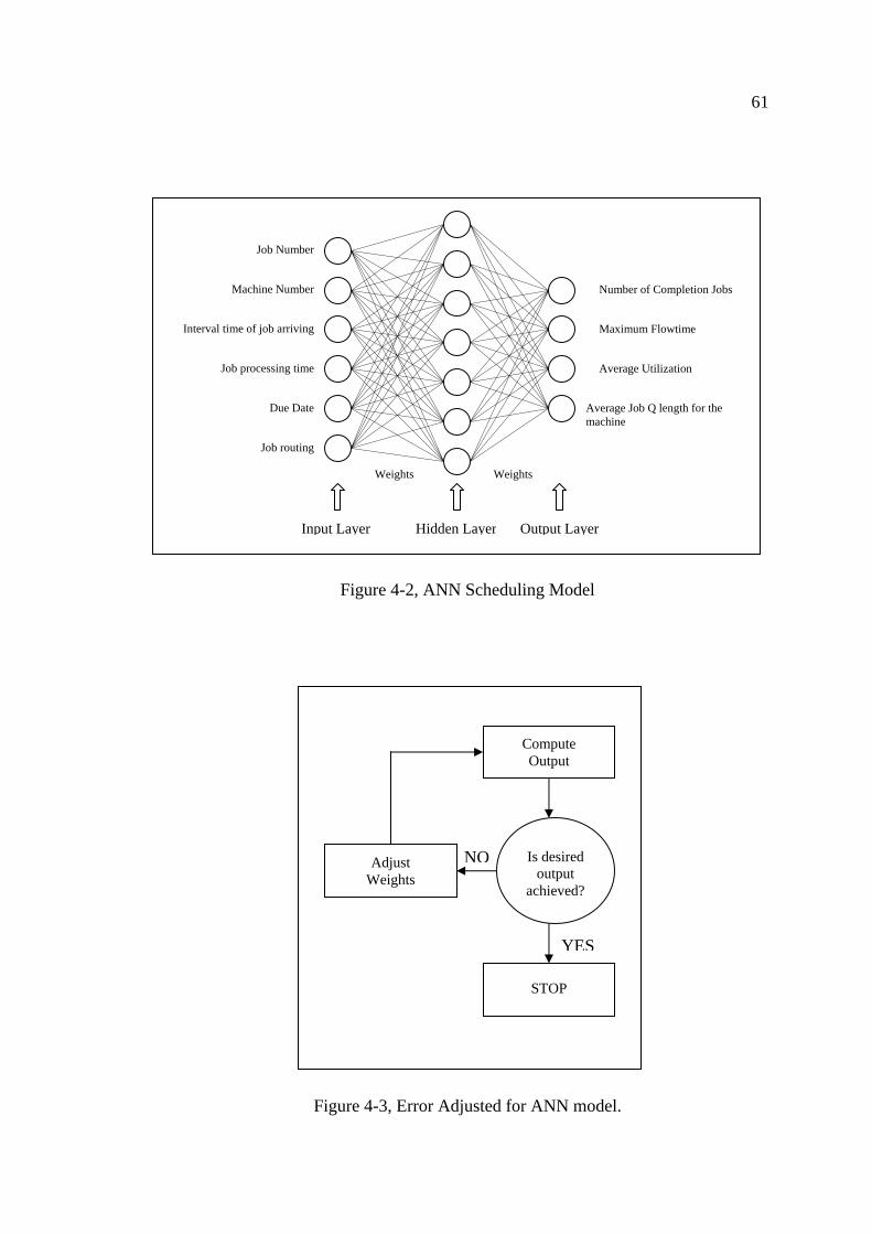
61

Figure 4-2, ANN Scheduling Model

Figure 4-3, Error Adjusted for ANN model.

Compute Output

Adjust Weights

STOP

Is desired output

achieved?

NO

YES

Number of Completion Jobs

Average Job Q length for the machine

Maximum Flowtime

Average Utilization

Job Number

Machine Number

Interval time of job arriving

Job processing time

Due Date

Job routing

Input Layer Hidden Layer Output Layer

Weights Weights

62

4.4 Sequence Codification Scheme (SCS)

The ANN structure with one input layer, one hidden layer, and one output

layer as shown in Figure 4-2 was used in this study. Data representation is an

important issue that directly influences the decision on the ANN architecture,

specifically, the number of input neurons. The number of input neurons required to

represent any given job sequence depends on the definition of these sequence

codification scheme (SCS). The codification rules adopted in this research was based

on the guidelines proposed by Lawrence (1994). A brief description of the SCS is

provided in the Appendix E.

CHAPTER 5

RESULTS AND DISCUSSION

5.1 Simulation Results

This chapter provides training results for the ANN scheduling model. Tables 5.1 to

5.9 present the results for FIFO, EDD, and SPT scheduling rules with the respective

“Low”, “Medium”, and “High” job arrivals. Appendix B provides the flowcharts for FIFO,

SPT, and EDD algorithm.

5.2 ANN Training Results

The scheduling scenarios evaluated through ARENA simulation provided valuable

input data sets and they were used for training the ANN scheduling model. Detailed results

from ARENA simulation are provided in Appendix D.

The training parameters used for the ANN model is shown in Table 5-10. A total of

180 training samples were used with a learning rate = 0.1.

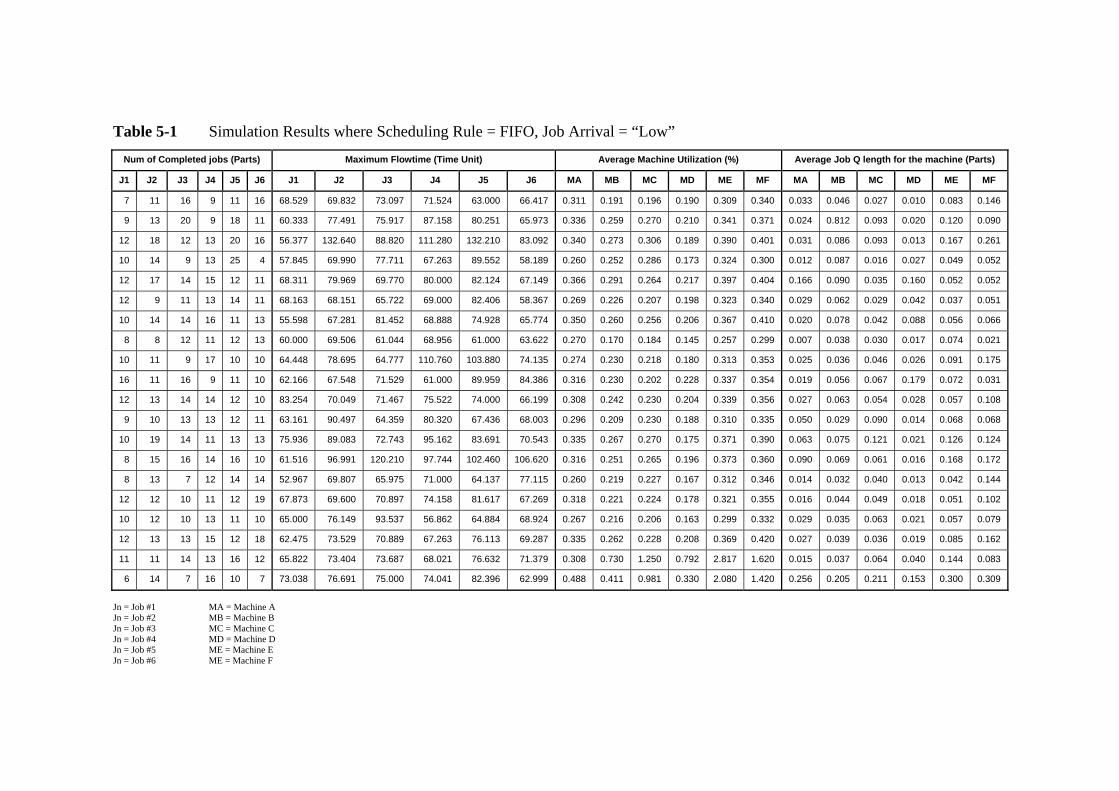
Table 5-1 Simulation Results where Scheduling Rule = FIFO, Job Arrival = “Low” Num of Completed jobs (Parts) Maximum Flowtime (Time Unit) Average Machine Utilization (%) Average Job Q length for the machine (Parts)

J1 J2 J3 J4 J5 J6 J1 J2 J3 J4 J5 J6 MA MB MC MD ME MF MA MB MC MD ME MF

7 11 16 9 11 16 68.529 69.832 73.097 71.524 63.000 66.417 0.311 0.191 0.196 0.190 0.309 0.340 0.033 0.046 0.027 0.010 0.083 0.146

9 13 20 9 18 11 60.333 77.491 75.917 87.158 80.251 65.973 0.336 0.259 0.270 0.210 0.341 0.371 0.024 0.812 0.093 0.020 0.120 0.090

12 18 12 13 20 16 56.377 132.640 88.820 111.280 132.210 83.092 0.340 0.273 0.306 0.189 0.390 0.401 0.031 0.086 0.093 0.013 0.167 0.261

10 14 9 13 25 4 57.845 69.990 77.711 67.263 89.552 58.189 0.260 0.252 0.286 0.173 0.324 0.300 0.012 0.087 0.016 0.027 0.049 0.052

12 17 14 15 12 11 68.311 79.969 69.770 80.000 82.124 67.149 0.366 0.291 0.264 0.217 0.397 0.404 0.166 0.090 0.035 0.160 0.052 0.052

12 9 11 13 14 11 68.163 68.151 65.722 69.000 82.406 58.367 0.269 0.226 0.207 0.198 0.323 0.340 0.029 0.062 0.029 0.042 0.037 0.051

10 14 14 16 11 13 55.598 67.281 81.452 68.888 74.928 65.774 0.350 0.260 0.256 0.206 0.367 0.410 0.020 0.078 0.042 0.088 0.056 0.066

8 8 12 11 12 13 60.000 69.506 61.044 68.956 61.000 63.622 0.270 0.170 0.184 0.145 0.257 0.299 0.007 0.038 0.030 0.017 0.074 0.021

10 11 9 17 10 10 64.448 78.695 64.777 110.760 103.880 74.135 0.274 0.230 0.218 0.180 0.313 0.353 0.025 0.036 0.046 0.026 0.091 0.175

16 11 16 9 11 10 62.166 67.548 71.529 61.000 89.959 84.386 0.316 0.230 0.202 0.228 0.337 0.354 0.019 0.056 0.067 0.179 0.072 0.031

12 13 14 14 12 10 83.254 70.049 71.467 75.522 74.000 66.199 0.308 0.242 0.230 0.204 0.339 0.356 0.027 0.063 0.054 0.028 0.057 0.108

9 10 13 13 12 11 63.161 90.497 64.359 80.320 67.436 68.003 0.296 0.209 0.230 0.188 0.310 0.335 0.050 0.029 0.090 0.014 0.068 0.068

10 19 14 11 13 13 75.936 89.083 72.743 95.162 83.691 70.543 0.335 0.267 0.270 0.175 0.371 0.390 0.063 0.075 0.121 0.021 0.126 0.124

8 15 16 14 16 10 61.516 96.991 120.210 97.744 102.460 106.620 0.316 0.251 0.265 0.196 0.373 0.360 0.090 0.069 0.061 0.016 0.168 0.172

8 13 7 12 14 14 52.967 69.807 65.975 71.000 64.137 77.115 0.260 0.219 0.227 0.167 0.312 0.346 0.014 0.032 0.040 0.013 0.042 0.144

12 12 10 11 12 19 67.873 69.600 70.897 74.158 81.617 67.269 0.318 0.221 0.224 0.178 0.321 0.355 0.016 0.044 0.049 0.018 0.051 0.102

10 12 10 13 11 10 65.000 76.149 93.537 56.862 64.884 68.924 0.267 0.216 0.206 0.163 0.299 0.332 0.029 0.035 0.063 0.021 0.057 0.079

12 13 13 15 12 18 62.475 73.529 70.889 67.263 76.113 69.287 0.335 0.262 0.228 0.208 0.369 0.420 0.027 0.039 0.036 0.019 0.085 0.162

11 11 14 13 16 12 65.822 73.404 73.687 68.021 76.632 71.379 0.308 0.730 1.250 0.792 2.817 1.620 0.015 0.037 0.064 0.040 0.144 0.083

6 14 7 16 10 7 73.038 76.691 75.000 74.041 82.396 62.999 0.488 0.411 0.981 0.330 2.080 1.420 0.256 0.205 0.211 0.153 0.300 0.309

Jn = Job #1 MA = Machine A Jn = Job #2 MB = Machine B Jn = Job #3 MC = Machine C Jn = Job #4 MD = Machine D Jn = Job #5 ME = Machine E Jn = Job #6 ME = Machine F

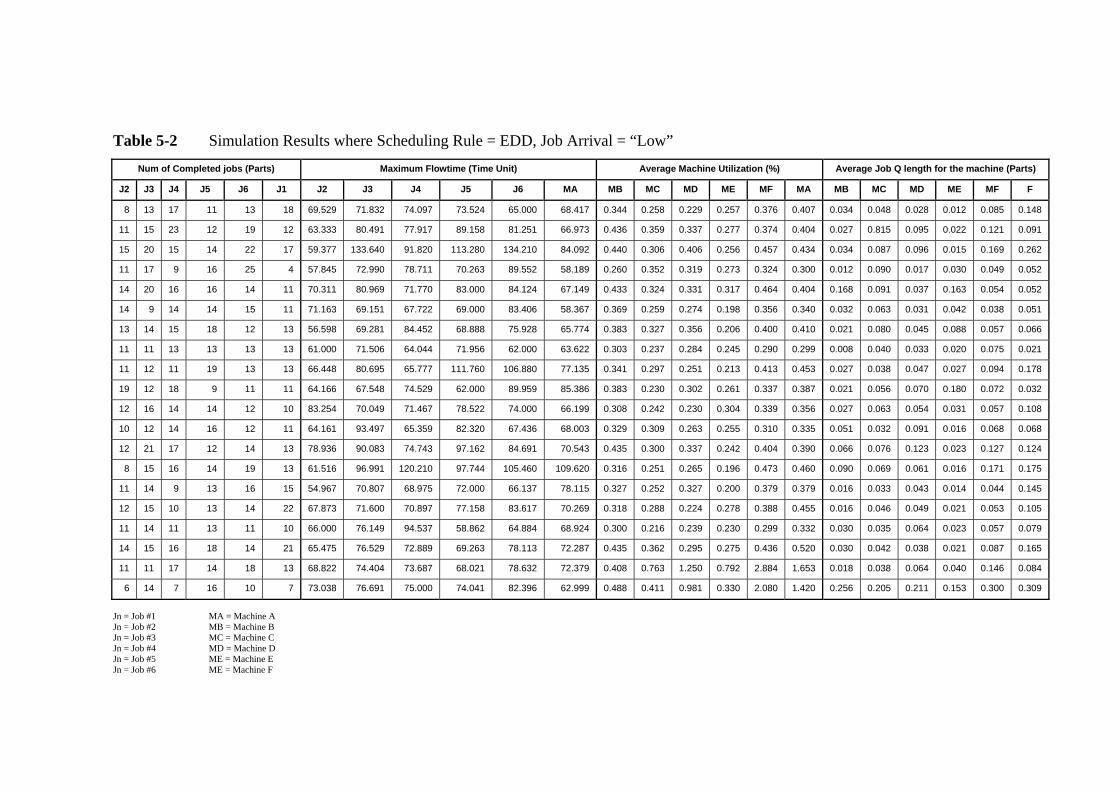
Table 5-2 Simulation Results where Scheduling Rule = EDD, Job Arrival = “Low”

Num of Completed jobs (Parts) Maximum Flowtime (Time Unit) Average Machine Utilization (%) Average Job Q length for the machine (Parts)

J2 J3 J4 J5 J6 J1 J2 J3 J4 J5 J6 MA MB MC MD ME MF MA MB MC MD ME MF F

8 13 17 11 13 18 69.529 71.832 74.097 73.524 65.000 68.417 0.344 0.258 0.229 0.257 0.376 0.407 0.034 0.048 0.028 0.012 0.085 0.148

11 15 23 12 19 12 63.333 80.491 77.917 89.158 81.251 66.973 0.436 0.359 0.337 0.277 0.374 0.404 0.027 0.815 0.095 0.022 0.121 0.091

15 20 15 14 22 17 59.377 133.640 91.820 113.280 134.210 84.092 0.440 0.306 0.406 0.256 0.457 0.434 0.034 0.087 0.096 0.015 0.169 0.262

11 17 9 16 25 4 57.845 72.990 78.711 70.263 89.552 58.189 0.260 0.352 0.319 0.273 0.324 0.300 0.012 0.090 0.017 0.030 0.049 0.052

14 20 16 16 14 11 70.311 80.969 71.770 83.000 84.124 67.149 0.433 0.324 0.331 0.317 0.464 0.404 0.168 0.091 0.037 0.163 0.054 0.052

14 9 14 14 15 11 71.163 69.151 67.722 69.000 83.406 58.367 0.369 0.259 0.274 0.198 0.356 0.340 0.032 0.063 0.031 0.042 0.038 0.051

13 14 15 18 12 13 56.598 69.281 84.452 68.888 75.928 65.774 0.383 0.327 0.356 0.206 0.400 0.410 0.021 0.080 0.045 0.088 0.057 0.066

11 11 13 13 13 13 61.000 71.506 64.044 71.956 62.000 63.622 0.303 0.237 0.284 0.245 0.290 0.299 0.008 0.040 0.033 0.020 0.075 0.021

11 12 11 19 13 13 66.448 80.695 65.777 111.760 106.880 77.135 0.341 0.297 0.251 0.213 0.413 0.453 0.027 0.038 0.047 0.027 0.094 0.178

19 12 18 9 11 11 64.166 67.548 74.529 62.000 89.959 85.386 0.383 0.230 0.302 0.261 0.337 0.387 0.021 0.056 0.070 0.180 0.072 0.032

12 16 14 14 12 10 83.254 70.049 71.467 78.522 74.000 66.199 0.308 0.242 0.230 0.304 0.339 0.356 0.027 0.063 0.054 0.031 0.057 0.108

10 12 14 16 12 11 64.161 93.497 65.359 82.320 67.436 68.003 0.329 0.309 0.263 0.255 0.310 0.335 0.051 0.032 0.091 0.016 0.068 0.068

12 21 17 12 14 13 78.936 90.083 74.743 97.162 84.691 70.543 0.435 0.300 0.337 0.242 0.404 0.390 0.066 0.076 0.123 0.023 0.127 0.124

8 15 16 14 19 13 61.516 96.991 120.210 97.744 105.460 109.620 0.316 0.251 0.265 0.196 0.473 0.460 0.090 0.069 0.061 0.016 0.171 0.175

11 14 9 13 16 15 54.967 70.807 68.975 72.000 66.137 78.115 0.327 0.252 0.327 0.200 0.379 0.379 0.016 0.033 0.043 0.014 0.044 0.145

12 15 10 13 14 22 67.873 71.600 70.897 77.158 83.617 70.269 0.318 0.288 0.224 0.278 0.388 0.455 0.016 0.046 0.049 0.021 0.053 0.105

11 14 11 13 11 10 66.000 76.149 94.537 58.862 64.884 68.924 0.300 0.216 0.239 0.230 0.299 0.332 0.030 0.035 0.064 0.023 0.057 0.079

14 15 16 18 14 21 65.475 76.529 72.889 69.263 78.113 72.287 0.435 0.362 0.295 0.275 0.436 0.520 0.030 0.042 0.038 0.021 0.087 0.165

11 11 17 14 18 13 68.822 74.404 73.687 68.021 78.632 72.379 0.408 0.763 1.250 0.792 2.884 1.653 0.018 0.038 0.064 0.040 0.146 0.084

6 14 7 16 10 7 73.038 76.691 75.000 74.041 82.396 62.999 0.488 0.411 0.981 0.330 2.080 1.420 0.256 0.205 0.211 0.153 0.300 0.309

Jn = Job #1 MA = Machine A Jn = Job #2 MB = Machine B Jn = Job #3 MC = Machine C Jn = Job #4 MD = Machine D Jn = Job #5 ME = Machine E Jn = Job #6 ME = Machine F

Table 5-3 Simulation Results where Scheduling Rule = SPT, Job Arrival = “Low” Num of Completed jobs (Parts) Maximum Flowtime (Time Unit) Average Machine Utilization (%) Average Job Q length for the machine (Parts)

J1 J2 J3 J4 J5 J6 J1 J2 J3 J4 J5 J6 MA MB MC MD ME MF MA MB MC MD ME MF

6 9 15 7 9 14 67.529 67.832 72.097 69.524 61.000 64.417 0.278 0.124 0.163 0.123 0.242 0.273 0.032 0.043 0.026 0.008 0.081 0.144

7 11 17 6 17 10 57.333 74.491 73.917 85.158 79.251 64.973 0.236 0.159 0.203 0.143 0.308 0.338 0.021 0.809 0.091 0.018 0.119 0.089

9 16 9 12 18 15 53.377 131.640 85.820 109.280 130.210 82.092 0.240 0.240 0.206 0.122 0.323 0.368 0.028 0.085 0.090 0.011 0.165 0.260

9 11 9 10 25 4 57.845 66.990 76.711 64.263 89.552 58.189 0.260 0.152 0.253 0.073 0.324 0.300 0.012 0.084 0.015 0.024 0.049 0.052

10 14 12 14 10 11 66.311 78.969 67.770 77.000 80.124 67.149 0.299 0.258 0.197 0.117 0.330 0.404 0.164 0.089 0.033 0.157 0.050 0.052

10 9 8 12 13 11 65.163 67.151 63.722 69.000 81.406 58.367 0.169 0.193 0.140 0.198 0.290 0.340 0.026 0.061 0.027 0.042 0.036 0.051

7 14 13 14 10 13 54.598 65.281 78.452 68.888 73.928 65.774 0.317 0.193 0.156 0.206 0.334 0.410 0.019 0.076 0.039 0.088 0.055 0.066

5 5 11 9 11 13 59.000 67.506 58.044 65.956 60.000 63.622 0.237 0.103 0.084 0.045 0.224 0.299 0.006 0.036 0.027 0.014 0.073 0.021

9 10 7 15 7 7 62.448 76.695 63.777 109.760 100.880 71.135 0.207 0.163 0.185 0.147 0.213 0.253 0.023 0.034 0.045 0.025 0.088 0.172

13 10 14 9 11 9 60.166 67.548 68.529 60.000 89.959 83.386 0.249 0.230 0.102 0.195 0.337 0.321 0.017 0.056 0.064 0.178 0.072 0.030

12 10 14 14 12 10 83.254 70.049 71.467 72.522 74.000 66.199 0.308 0.242 0.230 0.104 0.339 0.356 0.027 0.063 0.054 0.025 0.057 0.108

8 8 12 10 12 11 62.161 87.497 63.359 78.320 67.436 68.003 0.263 0.109 0.197 0.121 0.310 0.335 0.049 0.026 0.089 0.012 0.068 0.068

8 17 11 10 12 13 72.936 88.083 70.743 93.162 82.691 70.543 0.235 0.234 0.203 0.108 0.338 0.390 0.060 0.074 0.119 0.019 0.125 0.124

8 15 16 14 13 7 61.516 96.991 120.210 97.744 99.460 103.620 0.316 0.251 0.265 0.196 0.273 0.260 0.090 0.069 0.061 0.016 0.165 0.169

5 12 5 11 12 13 50.967 68.807 62.975 70.000 62.137 76.115 0.193 0.186 0.127 0.134 0.245 0.313 0.012 0.031 0.037 0.012 0.040 0.143

12 9 10 9 10 16 67.873 67.600 70.897 71.158 79.617 64.269 0.318 0.154 0.224 0.078 0.254 0.255 0.016 0.042 0.049 0.015 0.049 0.099

9 10 9 13 11 10 64.000 76.149 92.537 54.862 64.884 68.924 0.234 0.216 0.173 0.096 0.299 0.332 0.028 0.035 0.062 0.019 0.057 0.079

10 11 10 12 10 15 59.475 70.529 68.889 65.263 74.113 66.287 0.235 0.162 0.161 0.141 0.302 0.320 0.024 0.036 0.034 0.017 0.083 0.159

11 11 11 12 14 11 62.822 72.404 73.687 68.021 74.632 70.379 0.208 0.697 1.250 0.792 2.750 1.587 0.012 0.036 0.064 0.040 0.142 0.082

6 14 7 16 10 7 73.038 76.691 75.000 74.041 82.396 62.999 0.488 0.411 0.981 0.330 2.080 1.420 0.256 0.205 0.211 0.153 0.300 0.309

Jn = Job #1 MA = Machine A Jn = Job #2 MB = Machine B Jn = Job #3 MC = Machine C Jn = Job #4 MD = Machine D Jn = Job #5 ME = Machine E Jn = Job #6 ME = Machine F

Table 5-4 Simulation Results where Scheduling Rule = FIFO, Job Arrival = “Medium” Num of Completed jobs (Parts) Maximum Flowtime (Time Unit) Average Machine Utilization (%) Average Job Q length for the machine (Parts)

J1 J2 J3 J4 J5 J6 J1 J2 J3 J4 J5 J6 MA MB MC MD ME MF MA MB MC MD ME MF

21 23 22 30 26 27 73.162 77.137 75.349 68.000 123.190 88.243 0.548 0.471 0.434 0.370 0.633 0.696 0.975 0.127 0.109 0.086 0.296 0.497

19 25 32 20 30 22 69.117 80.157 77.291 75.420 78.520 100.130 0.563 0.458 0.476 0.346 0.652 0.676 0.129 0.137 0.182 0.050 0.334 0.382

26 28 17 27 29 21 63.528 70.138 64.570 69.590 127.100 129.980 0.522 0.497 0.413 0.375 0.634 0.667 0.107 0.168 0.118 0.067 0.341 0.520

18 32 16 39 38 9 93.196 72.873 75.171 76.371 131.380 130.600 0.510 0.529 0.514 0.339 0.716 0.660 0.092 0.182 0.205 0.085 0.402 0.295

23 28 27 29 26 17 83.249 80.503 93.652 79.158 135.240 117.360 0.599 0.496 0.458 0.385 0.687 0.667 0.216 0.193 0.191 0.076 0.416 0.423

28 31 16 31 29 20 75.681 82.620 78.238 75.822 102.480 165.400 0.550 0.525 0.455 0.383 0.693 0.662 0.128 0.188 0.173 0.073 0.457 0.450

21 19 23 31 30 26 83.000 71.887 77.010 78.021 97.461 92.361 0.516 0.470 0.488 0.327 0.648 0.661 0.096 0.125 0.231 0.043 0.281 0.436

19 19 22 31 36 27 65.218 69.837 81.248 68.004 92.979 101.470 0.536 0.468 0.500 0.351 0.656 0.675 0.090 0.118 0.200 0.072 0.374 0.414

16 31 24 28 29 25 84.098 81.137 83.476 72.620 81.102 110.440 0.552 0.486 0.480 0.334 0.664 0.692 0.097 0.146 0.198 0.065 0.288 0.399

27 23 23 29 25 24 68.965 73.749 80.684 65.395 84.173 82.746 0.516 0.472 0.423 0.379 0.650 0.633 0.102 0.154 0.146 0.062 0.244 0.402

22 27 25 28 19 28 77.584 75.171 76.497 72.127 78.887 90.236 0.582 0.466 0.394 0.384 0.652 0.727 0.088 0.110 0.126 0.075 0.318 0.526

22 25 28 23 33 24 85.087 82.318 80.709 80.915 109.850 120.860 0.578 0.483 0.492 0.353 0.662 0.693 0.191 0.151 0.243 0.063 0.447 0.503

23 31 25 22 29 23 84.062 80.855 71.356 82.649 157.230 116.540 0.574 0.485 0.486 0.358 0.673 0.692 0.109 0.122 0.213 0.048 0.299 0.565

18 26 34 26 31 20 90.444 86.984 92.983 70.783 98.421 127.420 0.539 0.437 0.484 0.359 0.662 0.670 0.087 0.149 0.169 0.072 0.386 0.427

16 42 18 21 25 23 102.860 78.607 86.486 74.865 75.786 121.730 0.562 0.531 0.452 0.339 0.671 0.694 0.148 0.207 0.231 0.074 0.422 0.486

20 15 29 32 26 29 90.941 81.708 88.445 65.858 88.710 97.379 0.558 0.425 0.448 0.341 0.620 0.677 0.118 0.122 0.186 0.055 0.285 0.473

15 22 30 31 31 27 74.573 77.856 80.151 73.534 110.020 109.190 0.579 0.463 0.501 0.338 0.654 0.705 0.162 0.208 0.197 0.038 0.299 0.529

27 27 29 23 26 22 77.286 95.107 80.134 68.390 98.357 99.360 0.552 0.486 0.424 0.392 0.635 0.677 0.137 0.105 0.148 0.120 0.302 0.475

22 24 28 23 27 23 96.983 87.132 71.989 69.649 110.110 116.030 0.552 0.447 0.442 0.364 0.616 0.670 0.068 0.140 0.138 0.057 0.276 0.432

23 22 16 33 33 26 67.204 74.426 82.529 69.696 91.024 106.640 0.554 0.485 0.482 0.328 0.677 0.637 0.099 0.112 0.260 0.046 0.252 0.350

Jn = Job #1 MA = Machine A Jn = Job #2 MB = Machine B Jn = Job #3 MC = Machine C Jn = Job #4 MD = Machine D Jn = Job #5 ME = Machine E Jn = Job #6 ME = Machine F

Table 5-5 Simulation Results where Scheduling Rule = EDD, Job Arrival = “Medium” Num of Completed jobs (Parts) Maximum Flowtime (Time Unit) Average Machine Utilization (%) Average Job Q length for the machine (Parts)

J1 J2 J3 J4 J5 J6 J1 J2 J3 J4 J5 J6 MA MB MC MD ME MF MA MB MC MD ME MF

22 25 23 32 28 29 74.162 79.137 76.349 70.000 125.190 90.243 0.648 0.671 0.534 0.570 0.833 0.896 0.985 0.147 0.119 0.106 0.316 0.517

21 27 35 23 31 23 72.117 83.157 79.291 77.420 79.520 101.130 0.863 0.758 0.676 0.546 0.752 0.776 0.159 0.167 0.202 0.070 0.344 0.392

29 30 20 28 31 22 66.528 71.138 67.570 71.590 129.100 130.980 0.822 0.597 0.713 0.575 0.834 0.767 0.137 0.178 0.148 0.087 0.361 0.530

19 35 16 42 38 9 93.196 75.873 76.171 79.371 131.380 130.600 0.510 0.829 0.614 0.639 0.716 0.660 0.092 0.212 0.215 0.115 0.402 0.295

25 31 29 30 28 17 85.249 81.503 95.652 82.158 137.240 117.360 0.799 0.596 0.658 0.685 0.887 0.667 0.236 0.203 0.211 0.106 0.436 0.423

30 31 19 32 30 20 78.681 83.620 80.238 75.822 103.480 165.400 0.850 0.625 0.655 0.383 0.793 0.662 0.158 0.198 0.193 0.073 0.467 0.450

24 19 24 33 31 26 84.000 73.887 80.010 78.021 98.461 92.361 0.616 0.670 0.788 0.327 0.748 0.661 0.106 0.145 0.261 0.043 0.291 0.436

22 22 23 33 37 27 66.218 71.837 84.248 71.004 93.979 101.470 0.636 0.668 0.800 0.651 0.756 0.675 0.100 0.138 0.230 0.102 0.384 0.414

17 32 26 30 32 28 86.098 83.137 84.476 73.620 84.102 113.440 0.752 0.686 0.580 0.434 0.964 0.992 0.117 0.166 0.208 0.075 0.318 0.429

30 24 25 29 25 25 70.965 73.749 83.684 66.395 84.173 83.746 0.716 0.472 0.723 0.479 0.650 0.733 0.122 0.154 0.176 0.072 0.244 0.412

22 30 25 28 19 28 77.584 75.171 76.497 75.127 78.887 90.236 0.582 0.466 0.394 0.684 0.652 0.727 0.088 0.110 0.126 0.105 0.318 0.526

23 27 29 26 33 24 86.087 85.318 81.709 82.915 109.850 120.860 0.678 0.783 0.592 0.553 0.662 0.693 0.201 0.181 0.253 0.083 0.447 0.503

25 33 28 23 30 23 87.062 81.855 73.356 84.649 158.230 116.540 0.874 0.585 0.686 0.558 0.773 0.692 0.139 0.132 0.233 0.068 0.309 0.565

18 26 34 26 34 23 90.444 86.984 92.983 70.783 101.421 130.420 0.539 0.437 0.484 0.359 0.962 0.970 0.087 0.149 0.169 0.072 0.416 0.457

19 43 20 22 27 24 104.860 79.607 89.486 75.865 77.786 122.730 0.762 0.631 0.752 0.439 0.871 0.794 0.168 0.217 0.261 0.084 0.442 0.496

20 18 29 34 28 32 90.941 83.708 88.445 68.858 90.710 100.379 0.558 0.625 0.448 0.641 0.820 0.977 0.118 0.142 0.186 0.085 0.305 0.503

16 24 31 31 31 27 75.573 77.856 81.151 75.534 110.020 109.190 0.679 0.463 0.601 0.538 0.654 0.705 0.172 0.208 0.207 0.058 0.299 0.529

29 29 32 26 28 25 80.286 98.107 82.134 70.390 100.357 102.360 0.852 0.786 0.624 0.592 0.835 0.977 0.167 0.135 0.168 0.140 0.322 0.505

22 24 31 24 29 24 99.983 88.132 71.989 69.649 112.110 117.030 0.852 0.547 0.442 0.364 0.816 0.770 0.098 0.150 0.138 0.057 0.296 0.442

23 22 16 33 33 26 67.204 74.426 82.529 69.696 91.024 106.640 0.554 0.485 0.482 0.328 0.677 0.637 0.099 0.112 0.260 0.046 0.252 0.350

Jn = Job #1 MA = Machine A Jn = Job #2 MB = Machine B Jn = Job #3 MC = Machine C Jn = Job #4 MD = Machine D Jn = Job #5 ME = Machine E Jn = Job #6 ME = Machine F

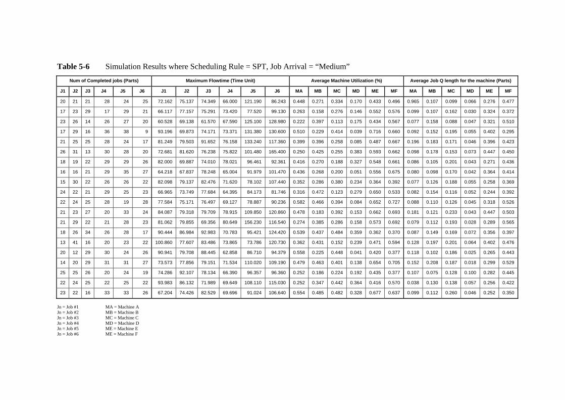
Table 5-6 Simulation Results where Scheduling Rule = SPT, Job Arrival = “Medium” Num of Completed jobs (Parts) Maximum Flowtime (Time Unit) Average Machine Utilization (%) Average Job Q length for the machine (Parts)

J1 J2 J3 J4 J5 J6 J1 J2 J3 J4 J5 J6 MA MB MC MD ME MF MA MB MC MD ME MF

20 21 21 28 24 25 72.162 75.137 74.349 66.000 121.190 86.243 0.448 0.271 0.334 0.170 0.433 0.496 0.965 0.107 0.099 0.066 0.276 0.477

17 23 29 17 29 21 66.117 77.157 75.291 73.420 77.520 99.130 0.263 0.158 0.276 0.146 0.552 0.576 0.099 0.107 0.162 0.030 0.324 0.372

23 26 14 26 27 20 60.528 69.138 61.570 67.590 125.100 128.980 0.222 0.397 0.113 0.175 0.434 0.567 0.077 0.158 0.088 0.047 0.321 0.510

17 29 16 36 38 9 93.196 69.873 74.171 73.371 131.380 130.600 0.510 0.229 0.414 0.039 0.716 0.660 0.092 0.152 0.195 0.055 0.402 0.295

21 25 25 28 24 17 81.249 79.503 91.652 76.158 133.240 117.360 0.399 0.396 0.258 0.085 0.487 0.667 0.196 0.183 0.171 0.046 0.396 0.423

26 31 13 30 28 20 72.681 81.620 76.238 75.822 101.480 165.400 0.250 0.425 0.255 0.383 0.593 0.662 0.098 0.178 0.153 0.073 0.447 0.450

18 19 22 29 29 26 82.000 69.887 74.010 78.021 96.461 92.361 0.416 0.270 0.188 0.327 0.548 0.661 0.086 0.105 0.201 0.043 0.271 0.436

16 16 21 29 35 27 64.218 67.837 78.248 65.004 91.979 101.470 0.436 0.268 0.200 0.051 0.556 0.675 0.080 0.098 0.170 0.042 0.364 0.414

15 30 22 26 26 22 82.098 79.137 82.476 71.620 78.102 107.440 0.352 0.286 0.380 0.234 0.364 0.392 0.077 0.126 0.188 0.055 0.258 0.369

24 22 21 29 25 23 66.965 73.749 77.684 64.395 84.173 81.746 0.316 0.472 0.123 0.279 0.650 0.533 0.082 0.154 0.116 0.052 0.244 0.392

22 24 25 28 19 28 77.584 75.171 76.497 69.127 78.887 90.236 0.582 0.466 0.394 0.084 0.652 0.727 0.088 0.110 0.126 0.045 0.318 0.526

21 23 27 20 33 24 84.087 79.318 79.709 78.915 109.850 120.860 0.478 0.183 0.392 0.153 0.662 0.693 0.181 0.121 0.233 0.043 0.447 0.503

21 29 22 21 28 23 81.062 79.855 69.356 80.649 156.230 116.540 0.274 0.385 0.286 0.158 0.573 0.692 0.079 0.112 0.193 0.028 0.289 0.565

18 26 34 26 28 17 90.444 86.984 92.983 70.783 95.421 124.420 0.539 0.437 0.484 0.359 0.362 0.370 0.087 0.149 0.169 0.072 0.356 0.397

13 41 16 20 23 22 100.860 77.607 83.486 73.865 73.786 120.730 0.362 0.431 0.152 0.239 0.471 0.594 0.128 0.197 0.201 0.064 0.402 0.476

20 12 29 30 24 26 90.941 79.708 88.445 62.858 86.710 94.379 0.558 0.225 0.448 0.041 0.420 0.377 0.118 0.102 0.186 0.025 0.265 0.443

14 20 29 31 31 27 73.573 77.856 79.151 71.534 110.020 109.190 0.479 0.463 0.401 0.138 0.654 0.705 0.152 0.208 0.187 0.018 0.299 0.529

25 25 26 20 24 19 74.286 92.107 78.134 66.390 96.357 96.360 0.252 0.186 0.224 0.192 0.435 0.377 0.107 0.075 0.128 0.100 0.282 0.445

22 24 25 22 25 22 93.983 86.132 71.989 69.649 108.110 115.030 0.252 0.347 0.442 0.364 0.416 0.570 0.038 0.130 0.138 0.057 0.256 0.422

23 22 16 33 33 26 67.204 74.426 82.529 69.696 91.024 106.640 0.554 0.485 0.482 0.328 0.677 0.637 0.099 0.112 0.260 0.046 0.252 0.350

Jn = Job #1 MA = Machine A Jn = Job #2 MB = Machine B Jn = Job #3 MC = Machine C Jn = Job #4 MD = Machine D Jn = Job #5 ME = Machine E Jn = Job #6 ME = Machine F

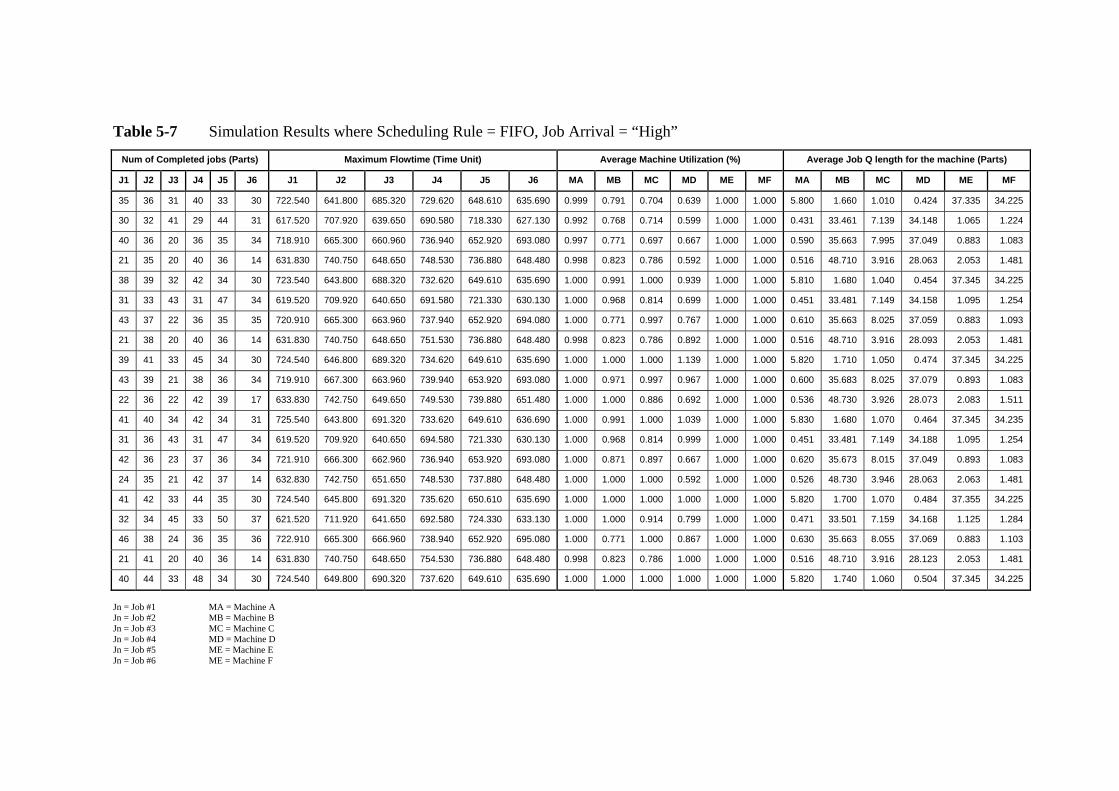
Table 5-7 Simulation Results where Scheduling Rule = FIFO, Job Arrival = “High” Num of Completed jobs (Parts) Maximum Flowtime (Time Unit) Average Machine Utilization (%) Average Job Q length for the machine (Parts)

J1 J2 J3 J4 J5 J6 J1 J2 J3 J4 J5 J6 MA MB MC MD ME MF MA MB MC MD ME MF

35 36 31 40 33 30 722.540 641.800 685.320 729.620 648.610 635.690 0.999 0.791 0.704 0.639 1.000 1.000 5.800 1.660 1.010 0.424 37.335 34.225

30 32 41 29 44 31 617.520 707.920 639.650 690.580 718.330 627.130 0.992 0.768 0.714 0.599 1.000 1.000 0.431 33.461 7.139 34.148 1.065 1.224

40 36 20 36 35 34 718.910 665.300 660.960 736.940 652.920 693.080 0.997 0.771 0.697 0.667 1.000 1.000 0.590 35.663 7.995 37.049 0.883 1.083

21 35 20 40 36 14 631.830 740.750 648.650 748.530 736.880 648.480 0.998 0.823 0.786 0.592 1.000 1.000 0.516 48.710 3.916 28.063 2.053 1.481

38 39 32 42 34 30 723.540 643.800 688.320 732.620 649.610 635.690 1.000 0.991 1.000 0.939 1.000 1.000 5.810 1.680 1.040 0.454 37.345 34.225

31 33 43 31 47 34 619.520 709.920 640.650 691.580 721.330 630.130 1.000 0.968 0.814 0.699 1.000 1.000 0.451 33.481 7.149 34.158 1.095 1.254

43 37 22 36 35 35 720.910 665.300 663.960 737.940 652.920 694.080 1.000 0.771 0.997 0.767 1.000 1.000 0.610 35.663 8.025 37.059 0.883 1.093

21 38 20 40 36 14 631.830 740.750 648.650 751.530 736.880 648.480 0.998 0.823 0.786 0.892 1.000 1.000 0.516 48.710 3.916 28.093 2.053 1.481

39 41 33 45 34 30 724.540 646.800 689.320 734.620 649.610 635.690 1.000 1.000 1.000 1.139 1.000 1.000 5.820 1.710 1.050 0.474 37.345 34.225

43 39 21 38 36 34 719.910 667.300 663.960 739.940 653.920 693.080 1.000 0.971 0.997 0.967 1.000 1.000 0.600 35.683 8.025 37.079 0.893 1.083

22 36 22 42 39 17 633.830 742.750 649.650 749.530 739.880 651.480 1.000 1.000 0.886 0.692 1.000 1.000 0.536 48.730 3.926 28.073 2.083 1.511

41 40 34 42 34 31 725.540 643.800 691.320 733.620 649.610 636.690 1.000 0.991 1.000 1.039 1.000 1.000 5.830 1.680 1.070 0.464 37.345 34.235

31 36 43 31 47 34 619.520 709.920 640.650 694.580 721.330 630.130 1.000 0.968 0.814 0.999 1.000 1.000 0.451 33.481 7.149 34.188 1.095 1.254

42 36 23 37 36 34 721.910 666.300 662.960 736.940 653.920 693.080 1.000 0.871 0.897 0.667 1.000 1.000 0.620 35.673 8.015 37.049 0.893 1.083

24 35 21 42 37 14 632.830 742.750 651.650 748.530 737.880 648.480 1.000 1.000 1.000 0.592 1.000 1.000 0.526 48.730 3.946 28.063 2.063 1.481

41 42 33 44 35 30 724.540 645.800 691.320 735.620 650.610 635.690 1.000 1.000 1.000 1.000 1.000 1.000 5.820 1.700 1.070 0.484 37.355 34.225

32 34 45 33 50 37 621.520 711.920 641.650 692.580 724.330 633.130 1.000 1.000 0.914 0.799 1.000 1.000 0.471 33.501 7.159 34.168 1.125 1.284

46 38 24 36 35 36 722.910 665.300 666.960 738.940 652.920 695.080 1.000 0.771 1.000 0.867 1.000 1.000 0.630 35.663 8.055 37.069 0.883 1.103

21 41 20 40 36 14 631.830 740.750 648.650 754.530 736.880 648.480 0.998 0.823 0.786 1.000 1.000 1.000 0.516 48.710 3.916 28.123 2.053 1.481

40 44 33 48 34 30 724.540 649.800 690.320 737.620 649.610 635.690 1.000 1.000 1.000 1.000 1.000 1.000 5.820 1.740 1.060 0.504 37.345 34.225

Jn = Job #1 MA = Machine A Jn = Job #2 MB = Machine B Jn = Job #3 MC = Machine C Jn = Job #4 MD = Machine D Jn = Job #5 ME = Machine E Jn = Job #6 ME = Machine F

Table 5-8 Simulation Results where Scheduling Rule = EDD, Job Arrival = “High” Num of Completed jobs (Parts) Maximum Flowtime (Time Unit) Average Machine Utilization (%) Average Job Q length for the machine (Parts)

J1 J2 J3 J4 J5 J6 J1 J2 J3 J4 J5 J6 MA MB MC MD ME MF MA MB MC MD ME MF

36 39 31 43 33 30 722.540 644.800 686.320 732.620 648.610 635.690 0.999 1.000 0.804 0.939 1.000 1.000 5.800 1.690 1.020 0.454 37.335 34.225

32 35 43 30 46 31 619.520 708.920 641.650 693.580 720.330 627.130 1.000 0.868 0.914 0.899 1.000 1.000 0.451 33.471 7.159 34.178 1.085 1.224

42 36 23 37 36 34 721.910 666.300 662.960 736.940 653.920 693.080 1.000 0.871 0.897 0.667 1.000 1.000 0.620 35.673 8.015 37.049 0.893 1.083

24 35 21 42 37 14 632.830 742.750 651.650 748.530 737.880 648.480 1.000 1.000 1.000 0.592 1.000 1.000 0.526 48.730 3.946 28.063 2.063 1.481

41 42 33 44 35 30 724.540 645.800 691.320 735.620 650.610 635.690 1.000 1.000 1.000 1.000 1.000 1.000 5.820 1.700 1.070 0.484 37.355 34.225

32 34 45 33 50 37 621.520 711.920 641.650 692.580 724.330 633.130 1.000 1.000 0.914 0.799 1.000 1.000 0.471 33.501 7.159 34.168 1.125 1.284

46 38 24 36 35 36 722.910 665.300 666.960 738.940 652.920 695.080 1.000 0.771 1.000 0.867 1.000 1.000 0.630 35.663 8.055 37.069 0.883 1.103

21 41 20 40 36 14 631.830 740.750 648.650 754.530 736.880 648.480 0.998 0.823 0.786 1.000 1.000 1.000 0.516 48.710 3.916 28.123 2.053 1.481

40 44 33 48 34 30 724.540 649.800 690.320 737.620 649.610 635.690 1.000 1.000 1.000 1.000 1.000 1.000 5.820 1.740 1.060 0.504 37.345 34.225

45 42 23 39 38 34 721.910 668.300 665.960 742.940 655.920 693.080 1.000 1.000 1.000 1.000 1.000 1.000 0.620 35.693 8.045 37.109 0.913 1.083

24 36 25 43 40 17 636.830 743.750 651.650 749.530 740.880 651.480 1.000 1.000 1.000 0.692 1.000 1.000 0.566 48.740 3.946 28.073 2.093 1.511

44 40 35 44 35 31 726.540 645.800 694.320 733.620 650.610 636.690 1.000 1.000 1.000 1.000 1.000 1.000 5.840 1.700 1.100 0.464 37.355 34.235

34 39 44 33 48 34 620.520 711.920 643.650 697.580 722.330 630.130 1.000 1.000 1.000 1.000 1.000 1.000 0.461 33.501 7.179 34.218 1.105 1.254

43 37 25 39 39 37 723.910 668.300 663.960 737.940 656.920 696.080 1.000 1.000 0.997 0.767 1.000 1.000 0.640 35.693 8.025 37.059 0.923 1.113

27 36 23 42 37 15 634.830 742.750 654.650 749.530 737.880 649.480 1.000 1.000 1.000 0.692 1.000 1.000 0.546 48.730 3.976 28.073 2.063 1.491

41 45 33 44 35 30 724.540 645.800 691.320 738.620 650.610 635.690 1.000 1.000 1.000 1.000 1.000 1.000 5.820 1.700 1.070 0.514 37.355 34.225

33 36 46 36 50 37 622.520 714.920 642.650 694.580 724.330 633.130 1.000 1.000 1.000 0.999 1.000 1.000 0.481 33.531 7.169 34.188 1.125 1.284

48 40 27 37 36 36 725.910 666.300 668.960 740.940 653.920 695.080 1.000 0.871 1.000 1.000 1.000 1.000 0.660 35.673 8.075 37.089 0.893 1.103

22 43 21 43 36 14 632.830 743.750 649.650 756.530 736.880 648.480 1.000 1.000 0.886 1.000 1.000 1.000 0.526 48.740 3.926 28.143 2.053 1.481

42 46 36 49 35 30 727.540 650.800 692.320 739.620 650.610 635.690 1.000 1.000 1.000 1.000 1.000 1.000 5.850 1.750 1.080 0.524 37.355 34.225

Jn = Job #1 MA = Machine A Jn = Job #2 MB = Machine B Jn = Job #3 MC = Machine C Jn = Job #4 MD = Machine D Jn = Job #5 ME = Machine E Jn = Job #6 ME = Machine F

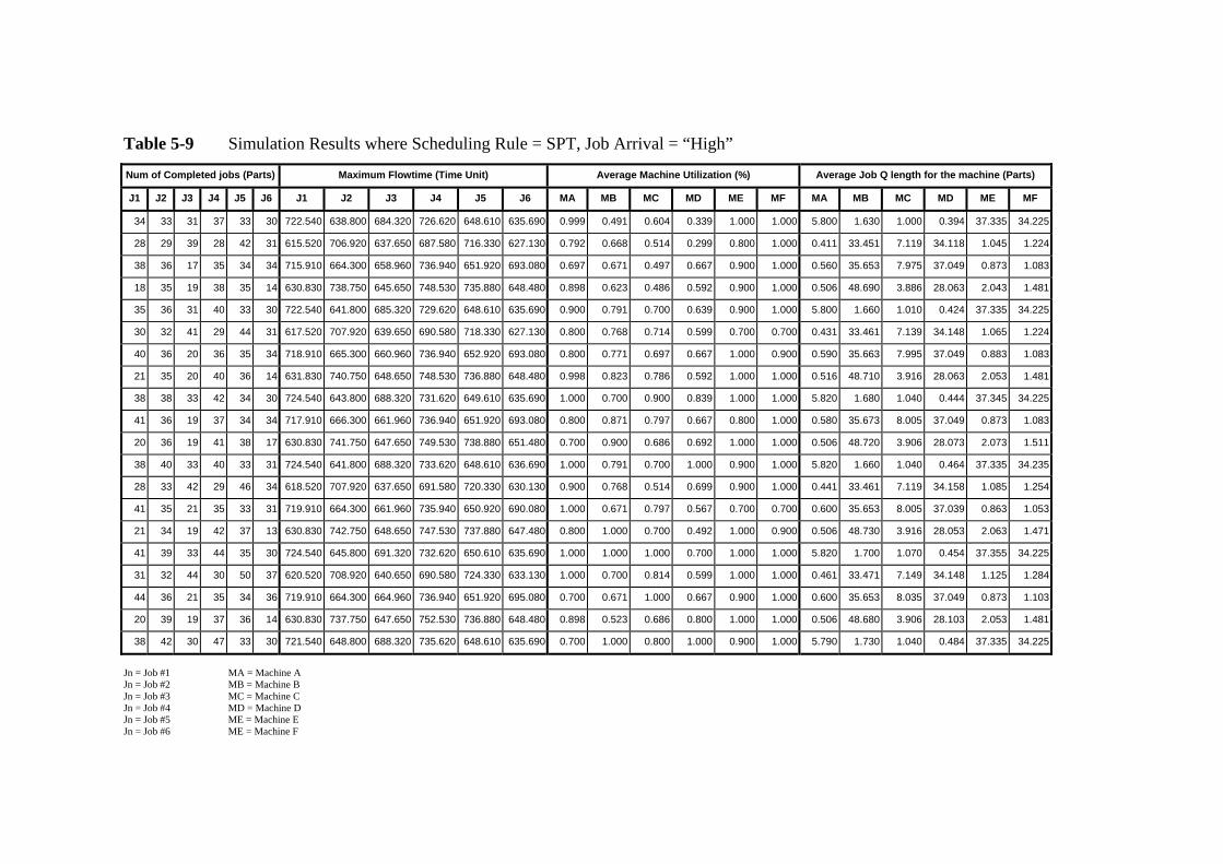
Table 5-9 Simulation Results where Scheduling Rule = SPT, Job Arrival = “High”

Num of Completed jobs (Parts) Maximum Flowtime (Time Unit) Average Machine Utilization (%) Average Job Q length for the machine (Parts)

J1 J2 J3 J4 J5 J6 J1 J2 J3 J4 J5 J6 MA MB MC MD ME MF MA MB MC MD ME MF

34 33 31 37 33 30 722.540 638.800 684.320 726.620 648.610 635.690 0.999 0.491 0.604 0.339 1.000 1.000 5.800 1.630 1.000 0.394 37.335 34.225

28 29 39 28 42 31 615.520 706.920 637.650 687.580 716.330 627.130 0.792 0.668 0.514 0.299 0.800 1.000 0.411 33.451 7.119 34.118 1.045 1.224

38 36 17 35 34 34 715.910 664.300 658.960 736.940 651.920 693.080 0.697 0.671 0.497 0.667 0.900 1.000 0.560 35.653 7.975 37.049 0.873 1.083

18 35 19 38 35 14 630.830 738.750 645.650 748.530 735.880 648.480 0.898 0.623 0.486 0.592 0.900 1.000 0.506 48.690 3.886 28.063 2.043 1.481

35 36 31 40 33 30 722.540 641.800 685.320 729.620 648.610 635.690 0.900 0.791 0.700 0.639 0.900 1.000 5.800 1.660 1.010 0.424 37.335 34.225

30 32 41 29 44 31 617.520 707.920 639.650 690.580 718.330 627.130 0.800 0.768 0.714 0.599 0.700 0.700 0.431 33.461 7.139 34.148 1.065 1.224

40 36 20 36 35 34 718.910 665.300 660.960 736.940 652.920 693.080 0.800 0.771 0.697 0.667 1.000 0.900 0.590 35.663 7.995 37.049 0.883 1.083

21 35 20 40 36 14 631.830 740.750 648.650 748.530 736.880 648.480 0.998 0.823 0.786 0.592 1.000 1.000 0.516 48.710 3.916 28.063 2.053 1.481

38 38 33 42 34 30 724.540 643.800 688.320 731.620 649.610 635.690 1.000 0.700 0.900 0.839 1.000 1.000 5.820 1.680 1.040 0.444 37.345 34.225

41 36 19 37 34 34 717.910 666.300 661.960 736.940 651.920 693.080 0.800 0.871 0.797 0.667 0.800 1.000 0.580 35.673 8.005 37.049 0.873 1.083

20 36 19 41 38 17 630.830 741.750 647.650 749.530 738.880 651.480 0.700 0.900 0.686 0.692 1.000 1.000 0.506 48.720 3.906 28.073 2.073 1.511

38 40 33 40 33 31 724.540 641.800 688.320 733.620 648.610 636.690 1.000 0.791 0.700 1.000 0.900 1.000 5.820 1.660 1.040 0.464 37.335 34.235

28 33 42 29 46 34 618.520 707.920 637.650 691.580 720.330 630.130 0.900 0.768 0.514 0.699 0.900 1.000 0.441 33.461 7.119 34.158 1.085 1.254

41 35 21 35 33 31 719.910 664.300 661.960 735.940 650.920 690.080 1.000 0.671 0.797 0.567 0.700 0.700 0.600 35.653 8.005 37.039 0.863 1.053

21 34 19 42 37 13 630.830 742.750 648.650 747.530 737.880 647.480 0.800 1.000 0.700 0.492 1.000 0.900 0.506 48.730 3.916 28.053 2.063 1.471

41 39 33 44 35 30 724.540 645.800 691.320 732.620 650.610 635.690 1.000 1.000 1.000 0.700 1.000 1.000 5.820 1.700 1.070 0.454 37.355 34.225

31 32 44 30 50 37 620.520 708.920 640.650 690.580 724.330 633.130 1.000 0.700 0.814 0.599 1.000 1.000 0.461 33.471 7.149 34.148 1.125 1.284

44 36 21 35 34 36 719.910 664.300 664.960 736.940 651.920 695.080 0.700 0.671 1.000 0.667 0.900 1.000 0.600 35.653 8.035 37.049 0.873 1.103

20 39 19 37 36 14 630.830 737.750 647.650 752.530 736.880 648.480 0.898 0.523 0.686 0.800 1.000 1.000 0.506 48.680 3.906 28.103 2.053 1.481

38 42 30 47 33 30 721.540 648.800 688.320 735.620 648.610 635.690 0.700 1.000 0.800 1.000 0.900 1.000 5.790 1.730 1.040 0.484 37.335 34.225

Jn = Job #1 MA = Machine A Jn = Job #2 MB = Machine B Jn = Job #3 MC = Machine C Jn = Job #4 MD = Machine D Jn = Job #5 ME = Machine E Jn = Job #6 ME = Machine F

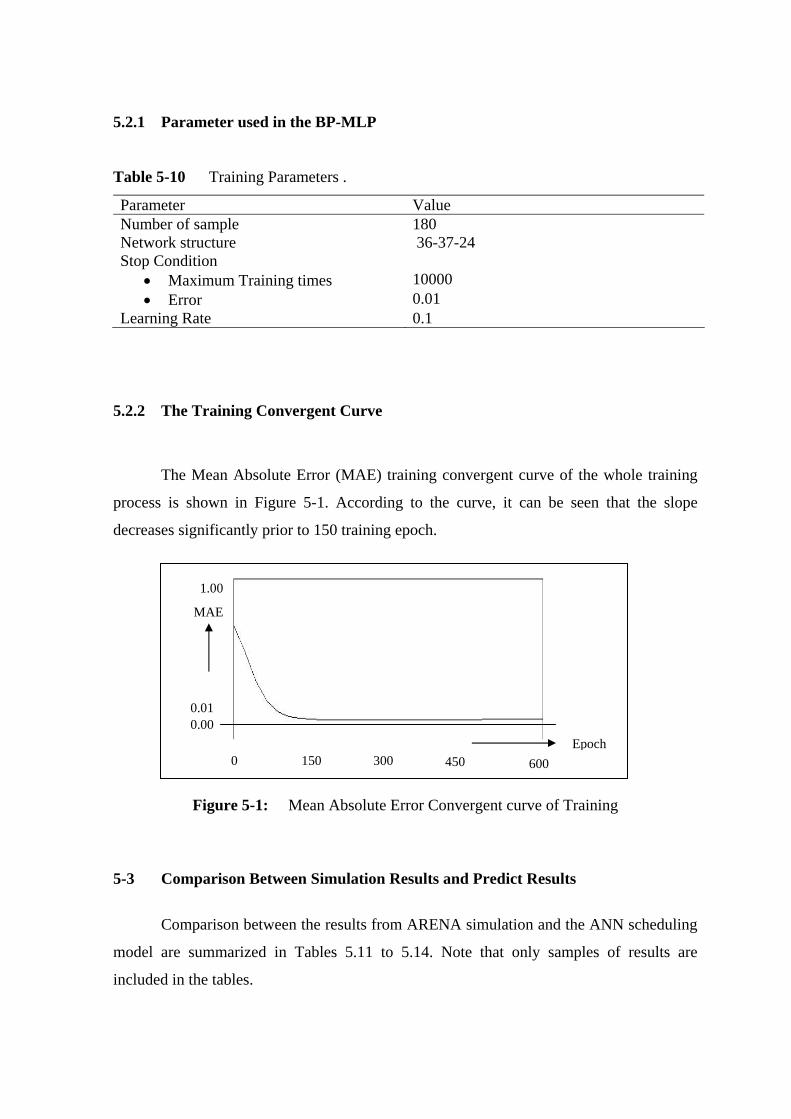
5.2.1 Parameter used in the BP-MLP

Table 5-10 Training Parameters .

Parameter Value Number of sample 180 Network structure 36-37-24 Stop Condition

• Maximum Training times 10000 • Error 0.01

Learning Rate 0.1

5.2.2 The Training Convergent Curve

The Mean Absolute Error (MAE) training convergent curve of the whole training

process is shown in Figure 5-1. According to the curve, it can be seen that the slope

decreases significantly prior to 150 training epoch.

Figure 5-1: Mean Absolute Error Convergent curve of Training

5-3 Comparison Between Simulation Results and Predict Results

Comparison between the results from ARENA simulation and the ANN scheduling

model are summarized in Tables 5.11 to 5.14. Note that only samples of results are

included in the tables.

1.00

0.01 0.00

0 300150 450 600Epoch

MAE

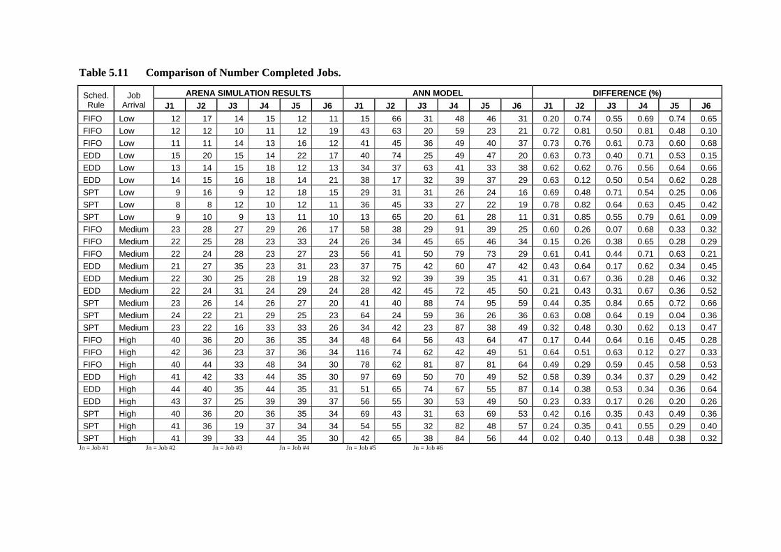
Table 5.11 Comparison of Number Completed Jobs.

ARENA SIMULATION RESULTS ANN MODEL DIFFERENCE (%) Sched. Rule

Job Arrival J1 J2 J3 J4 J5 J6 J1 J2 J3 J4 J5 J6 J1 J2 J3 J4 J5 J6

FIFO Low 12 17 14 15 12 11 15 66 31 48 46 31 0.20 0.74 0.55 0.69 0.74 0.65 FIFO Low 12 12 10 11 12 19 43 63 20 59 23 21 0.72 0.81 0.50 0.81 0.48 0.10 FIFO Low 11 11 14 13 16 12 41 45 36 49 40 37 0.73 0.76 0.61 0.73 0.60 0.68 EDD Low 15 20 15 14 22 17 40 74 25 49 47 20 0.63 0.73 0.40 0.71 0.53 0.15 EDD Low 13 14 15 18 12 13 34 37 63 41 33 38 0.62 0.62 0.76 0.56 0.64 0.66 EDD Low 14 15 16 18 14 21 38 17 32 39 37 29 0.63 0.12 0.50 0.54 0.62 0.28 SPT Low 9 16 9 12 18 15 29 31 31 26 24 16 0.69 0.48 0.71 0.54 0.25 0.06 SPT Low 8 8 12 10 12 11 36 45 33 27 22 19 0.78 0.82 0.64 0.63 0.45 0.42 SPT Low 9 10 9 13 11 10 13 65 20 61 28 11 0.31 0.85 0.55 0.79 0.61 0.09 FIFO Medium 23 28 27 29 26 17 58 38 29 91 39 25 0.60 0.26 0.07 0.68 0.33 0.32 FIFO Medium 22 25 28 23 33 24 26 34 45 65 46 34 0.15 0.26 0.38 0.65 0.28 0.29 FIFO Medium 22 24 28 23 27 23 56 41 50 79 73 29 0.61 0.41 0.44 0.71 0.63 0.21 EDD Medium 21 27 35 23 31 23 37 75 42 60 47 42 0.43 0.64 0.17 0.62 0.34 0.45 EDD Medium 22 30 25 28 19 28 32 92 39 39 35 41 0.31 0.67 0.36 0.28 0.46 0.32 EDD Medium 22 24 31 24 29 24 28 42 45 72 45 50 0.21 0.43 0.31 0.67 0.36 0.52 SPT Medium 23 26 14 26 27 20 41 40 88 74 95 59 0.44 0.35 0.84 0.65 0.72 0.66 SPT Medium 24 22 21 29 25 23 64 24 59 36 26 36 0.63 0.08 0.64 0.19 0.04 0.36 SPT Medium 23 22 16 33 33 26 34 42 23 87 38 49 0.32 0.48 0.30 0.62 0.13 0.47 FIFO High 40 36 20 36 35 34 48 64 56 43 64 47 0.17 0.44 0.64 0.16 0.45 0.28 FIFO High 42 36 23 37 36 34 116 74 62 42 49 51 0.64 0.51 0.63 0.12 0.27 0.33 FIFO High 40 44 33 48 34 30 78 62 81 87 81 64 0.49 0.29 0.59 0.45 0.58 0.53 EDD High 41 42 33 44 35 30 97 69 50 70 49 52 0.58 0.39 0.34 0.37 0.29 0.42 EDD High 44 40 35 44 35 31 51 65 74 67 55 87 0.14 0.38 0.53 0.34 0.36 0.64 EDD High 43 37 25 39 39 37 56 55 30 53 49 50 0.23 0.33 0.17 0.26 0.20 0.26 SPT High 40 36 20 36 35 34 69 43 31 63 69 53 0.42 0.16 0.35 0.43 0.49 0.36 SPT High 41 36 19 37 34 34 54 55 32 82 48 57 0.24 0.35 0.41 0.55 0.29 0.40 SPT High 41 39 33 44 35 30 42 65 38 84 56 44 0.02 0.40 0.13 0.48 0.38 0.32

Jn = Job #1 Jn = Job #2 Jn = Job #3 Jn = Job #4 Jn = Job #5 Jn = Job #6

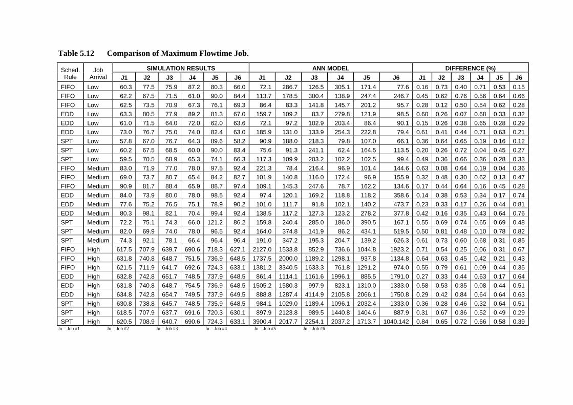
Table 5.12 Comparison of Maximum Flowtime Job.

SIMULATION RESULTS ANN MODEL DIFFERENCE (%) Sched. Rule

Job Arrival J1 J2 J3 J4 J5 J6 J1 J2 J3 J4 J5 J6 J1 J2 J3 J4 J5 J6

FIFO Low 60.3 77.5 75.9 87.2 80.3 66.0 72.1 286.7 126.5 305.1 171.4 77.6 0.16 0.73 0.40 0.71 0.53 0.15 FIFO Low 62.2 67.5 71.5 61.0 90.0 84.4 113.7 178.5 300.4 138.9 247.4 246.7 0.45 0.62 0.76 0.56 0.64 0.66 FIFO Low 62.5 73.5 70.9 67.3 76.1 69.3 86.4 83.3 141.8 145.7 201.2 95.7 0.28 0.12 0.50 0.54 0.62 0.28 EDD Low 63.3 80.5 77.9 89.2 81.3 67.0 159.7 109.2 83.7 279.8 121.9 98.5 0.60 0.26 0.07 0.68 0.33 0.32 EDD Low 61.0 71.5 64.0 72.0 62.0 63.6 72.1 97.2 102.9 203.4 86.4 90.1 0.15 0.26 0.38 0.65 0.28 0.29 EDD Low 73.0 76.7 75.0 74.0 82.4 63.0 185.9 131.0 133.9 254.3 222.8 79.4 0.61 0.41 0.44 0.71 0.63 0.21 SPT Low 57.8 67.0 76.7 64.3 89.6 58.2 90.9 188.0 218.3 79.8 107.0 66.1 0.36 0.64 0.65 0.19 0.16 0.12 SPT Low 60.2 67.5 68.5 60.0 90.0 83.4 75.6 91.3 241.1 62.4 164.5 113.5 0.20 0.26 0.72 0.04 0.45 0.27 SPT Low 59.5 70.5 68.9 65.3 74.1 66.3 117.3 109.9 203.2 102.2 102.5 99.4 0.49 0.36 0.66 0.36 0.28 0.33 FIFO Medium 83.0 71.9 77.0 78.0 97.5 92.4 221.3 78.4 216.4 96.9 101.4 144.6 0.63 0.08 0.64 0.19 0.04 0.36 FIFO Medium 69.0 73.7 80.7 65.4 84.2 82.7 101.9 140.8 116.0 172.4 96.9 155.9 0.32 0.48 0.30 0.62 0.13 0.47 FIFO Medium 90.9 81.7 88.4 65.9 88.7 97.4 109.1 145.3 247.6 78.7 162.2 134.6 0.17 0.44 0.64 0.16 0.45 0.28 EDD Medium 84.0 73.9 80.0 78.0 98.5 92.4 97.4 120.1 169.2 118.8 118.2 358.6 0.14 0.38 0.53 0.34 0.17 0.74 EDD Medium 77.6 75.2 76.5 75.1 78.9 90.2 101.0 111.7 91.8 102.1 140.2 473.7 0.23 0.33 0.17 0.26 0.44 0.81 EDD Medium 80.3 98.1 82.1 70.4 99.4 92.4 138.5 117.2 127.3 123.2 278.2 377.8 0.42 0.16 0.35 0.43 0.64 0.76 SPT Medium 72.2 75.1 74.3 66.0 121.2 86.2 159.8 240.4 285.0 186.0 390.5 167.1 0.55 0.69 0.74 0.65 0.69 0.48 SPT Medium 82.0 69.9 74.0 78.0 96.5 92.4 164.0 374.8 141.9 86.2 434.1 519.5 0.50 0.81 0.48 0.10 0.78 0.82 SPT Medium 74.3 92.1 78.1 66.4 96.4 96.4 191.0 347.2 195.3 204.7 139.2 626.3 0.61 0.73 0.60 0.68 0.31 0.85 FIFO High 617.5 707.9 639.7 690.6 718.3 627.1 2127.0 1533.8 852.9 736.6 1044.8 1923.2 0.71 0.54 0.25 0.06 0.31 0.67 FIFO High 631.8 740.8 648.7 751.5 736.9 648.5 1737.5 2000.0 1189.2 1298.1 937.8 1134.8 0.64 0.63 0.45 0.42 0.21 0.43 FIFO High 621.5 711.9 641.7 692.6 724.3 633.1 1381.2 3340.5 1633.3 761.8 1291.2 974.0 0.55 0.79 0.61 0.09 0.44 0.35 EDD High 632.8 742.8 651.7 748.5 737.9 648.5 861.4 1114.1 1161.6 1996.1 885.5 1791.0 0.27 0.33 0.44 0.63 0.17 0.64 EDD High 631.8 740.8 648.7 754.5 736.9 648.5 1505.2 1580.3 997.9 823.1 1310.0 1333.0 0.58 0.53 0.35 0.08 0.44 0.51 EDD High 634.8 742.8 654.7 749.5 737.9 649.5 888.8 1287.4 4114.9 2105.8 2066.1 1750.8 0.29 0.42 0.84 0.64 0.64 0.63 SPT High 630.8 738.8 645.7 748.5 735.9 648.5 984.1 1029.0 1189.4 1096.1 2032.4 1333.0 0.36 0.28 0.46 0.32 0.64 0.51 SPT High 618.5 707.9 637.7 691.6 720.3 630.1 897.9 2123.8 989.5 1440.8 1404.6 887.9 0.31 0.67 0.36 0.52 0.49 0.29 SPT High 620.5 708.9 640.7 690.6 724.3 633.1 3900.4 2017.7 2254.1 2037.2 1713.7 1040.142 0.84 0.65 0.72 0.66 0.58 0.39

Jn = Job #1 Jn = Job #2 Jn = Job #3 Jn = Job #4 Jn = Job #5 Jn = Job #6

Table 5.13 Comparison of Average Machine Utilization.

SIMULATION RESULTS ANN MODEL DIFFERENCE (%) Sched. Rule

Job Arrival MA MB MC MD ME MF MA MB MC MD ME MF MA MB MC MD ME MF

FIFO Low 0.336 0.259 0.270 0.210 0.341 0.371 0.358 0.447 0.297 0.309 0.483 0.468 0.06 0.42 0.09 0.32 0.29 0.21 FIFO Low 0.350 0.260 0.256 0.206 0.367 0.410 1.254 1.365 0.512 1.105 0.703 0.453 0.72 0.81 0.50 0.81 0.48 0.10 FIFO Low 0.318 0.221 0.224 0.178 0.321 0.355 1.185 0.904 0.576 0.671 0.803 1.095 0.73 0.76 0.61 0.73 0.60 0.68 EDD Low 0.344 0.258 0.229 0.257 0.376 0.407 0.918 0.953 0.382 0.898 0.803 0.478 0.63 0.73 0.40 0.71 0.53 0.15 EDD Low 0.329 0.309 0.263 0.255 0.310 0.335 0.861 0.817 1.106 0.580 0.853 0.979 0.62 0.62 0.76 0.56 0.64 0.66 EDD Low 0.318 0.288 0.224 0.278 0.388 0.455 0.863 0.326 0.448 0.602 1.025 0.628 0.63 0.12 0.50 0.54 0.62 0.28 SPT Low 0.299 0.258 0.197 0.117 0.330 0.404 0.965 0.499 0.680 0.254 0.440 0.431 0.69 0.48 0.71 0.54 0.25 0.06 SPT Low 0.308 0.242 0.230 0.104 0.339 0.356 1.386 1.361 0.633 0.281 0.622 0.615 0.78 0.82 0.64 0.63 0.45 0.42 SPT Low 0.318 0.154 0.224 0.078 0.254 0.255 0.459 1.003 0.498 0.366 0.647 0.281 0.31 0.85 0.55 0.79 0.61 0.09 FIFO Medium 0.563 0.458 0.476 0.346 0.652 0.676 1.420 0.622 0.511 1.086 0.978 0.994 0.60 0.26 0.07 0.68 0.33 0.32 FIFO Medium 0.552 0.486 0.480 0.334 0.664 0.692 0.652 0.661 0.771 0.944 0.926 0.980 0.15 0.26 0.38 0.65 0.28 0.29 FIFO Medium 0.579 0.463 0.501 0.338 0.654 0.705 1.474 0.791 0.895 1.161 1.768 0.889 0.61 0.41 0.44 0.71 0.63 0.21 EDD Medium 0.648 0.671 0.534 0.570 0.833 0.896 1.142 1.863 0.641 1.487 1.263 1.636 0.43 0.64 0.17 0.62 0.34 0.45 EDD Medium 0.582 0.466 0.394 0.684 0.652 0.727 0.847 1.429 0.615 0.953 1.201 1.065 0.31 0.67 0.36 0.28 0.46 0.32 EDD Medium 0.679 0.463 0.601 0.538 0.654 0.705 0.864 0.810 0.872 1.614 1.015 1.469 0.21 0.43 0.31 0.67 0.36 0.52 SPT Medium 0.510 0.229 0.414 0.039 0.716 0.660 0.909 0.352 2.602 0.111 2.519 1.947 0.44 0.35 0.84 0.65 0.72 0.66 SPT Medium 0.582 0.466 0.394 0.084 0.652 0.727 1.552 0.508 1.107 0.104 0.678 1.138 0.63 0.08 0.64 0.19 0.04 0.36 SPT Medium 0.554 0.485 0.482 0.328 0.677 0.637 0.819 0.926 0.693 0.865 0.780 1.201 0.32 0.48 0.30 0.62 0.13 0.47 FIFO High 0.999 0.791 0.704 0.639 1.000 1.000 1.199 1.406 1.971 0.763 1.829 1.382 0.17 0.44 0.64 0.16 0.45 0.28 FIFO High 0.998 0.823 0.786 0.892 1.000 1.000 2.756 1.692 2.119 1.013 1.361 1.500 0.64 0.51 0.63 0.12 0.27 0.33 FIFO High 0.998 0.823 0.786 1.000 1.000 1.000 1.946 1.160 1.929 1.813 2.382 2.133 0.49 0.29 0.59 0.45 0.58 0.53 EDD High 0.999 1.000 0.804 0.939 1.000 1.000 2.363 1.643 1.218 1.494 1.400 1.733 0.58 0.39 0.34 0.37 0.29 0.42 EDD High 0.998 0.823 0.786 1.000 1.000 1.000 1.157 1.337 1.662 1.523 1.571 2.806 0.14 0.38 0.53 0.34 0.36 0.64 EDD High 1.000 1.000 0.997 0.767 1.000 1.000 1.302 1.486 1.196 1.042 1.256 1.351 0.23 0.33 0.17 0.26 0.20 0.26 SPT High 0.792 0.668 0.514 0.299 0.800 1.000 1.366 0.798 0.797 0.523 1.577 1.559 0.42 0.16 0.35 0.43 0.49 0.36 SPT High 0.800 0.871 0.797 0.667 0.800 1.000 1.054 1.331 1.342 1.478 1.129 1.676 0.24 0.35 0.41 0.55 0.29 0.40 SPT High 0.898 0.523 0.686 0.800 1.000 1.000 0.920 0.872 0.790 1.527 1.600 1.467 0.02 0.40 0.13 0.48 0.38 0.32

MA = Machine A MB = Machine B MC = Machine C MD = Machine D ME = Machine E ME = Machine F

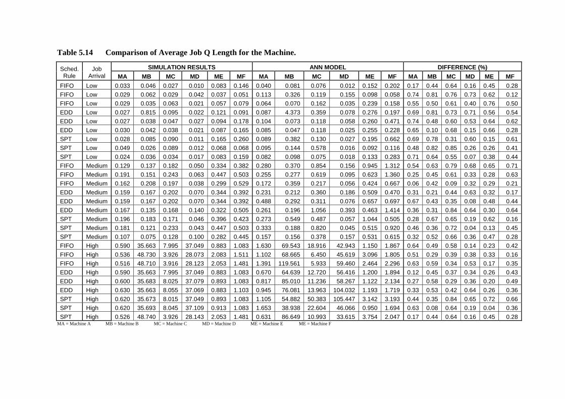
Table 5.14 Comparison of Average Job Q Length for the Machine.

SIMULATION RESULTS ANN MODEL DIFFERENCE (%) Sched. Rule

Job Arrival MA MB MC MD ME MF MA MB MC MD ME MF MA MB MC MD ME MF

FIFO Low 0.033 0.046 0.027 0.010 0.083 0.146 0.040 0.081 0.076 0.012 0.152 0.202 0.17 0.44 0.64 0.16 0.45 0.28 FIFO Low 0.029 0.062 0.029 0.042 0.037 0.051 0.113 0.326 0.119 0.155 0.098 0.058 0.74 0.81 0.76 0.73 0.62 0.12 FIFO Low 0.029 0.035 0.063 0.021 0.057 0.079 0.064 0.070 0.162 0.035 0.239 0.158 0.55 0.50 0.61 0.40 0.76 0.50 EDD Low 0.027 0.815 0.095 0.022 0.121 0.091 0.087 4.373 0.359 0.078 0.276 0.197 0.69 0.81 0.73 0.71 0.56 0.54 EDD Low 0.027 0.038 0.047 0.027 0.094 0.178 0.104 0.073 0.118 0.058 0.260 0.471 0.74 0.48 0.60 0.53 0.64 0.62 EDD Low 0.030 0.042 0.038 0.021 0.087 0.165 0.085 0.047 0.118 0.025 0.255 0.228 0.65 0.10 0.68 0.15 0.66 0.28 SPT Low 0.028 0.085 0.090 0.011 0.165 0.260 0.089 0.382 0.130 0.027 0.195 0.662 0.69 0.78 0.31 0.60 0.15 0.61 SPT Low 0.049 0.026 0.089 0.012 0.068 0.068 0.095 0.144 0.578 0.016 0.092 0.116 0.48 0.82 0.85 0.26 0.26 0.41 SPT Low 0.024 0.036 0.034 0.017 0.083 0.159 0.082 0.098 0.075 0.018 0.133 0.283 0.71 0.64 0.55 0.07 0.38 0.44 FIFO Medium 0.129 0.137 0.182 0.050 0.334 0.382 0.280 0.370 0.854 0.156 0.945 1.312 0.54 0.63 0.79 0.68 0.65 0.71 FIFO Medium 0.191 0.151 0.243 0.063 0.447 0.503 0.255 0.277 0.619 0.095 0.623 1.360 0.25 0.45 0.61 0.33 0.28 0.63 FIFO Medium 0.162 0.208 0.197 0.038 0.299 0.529 0.172 0.359 0.217 0.056 0.424 0.667 0.06 0.42 0.09 0.32 0.29 0.21 EDD Medium 0.159 0.167 0.202 0.070 0.344 0.392 0.231 0.212 0.360 0.186 0.509 0.470 0.31 0.21 0.44 0.63 0.32 0.17 EDD Medium 0.159 0.167 0.202 0.070 0.344 0.392 0.488 0.292 0.311 0.076 0.657 0.697 0.67 0.43 0.35 0.08 0.48 0.44 EDD Medium 0.167 0.135 0.168 0.140 0.322 0.505 0.261 0.196 1.056 0.393 0.463 1.414 0.36 0.31 0.84 0.64 0.30 0.64 SPT Medium 0.196 0.183 0.171 0.046 0.396 0.423 0.273 0.549 0.487 0.057 1.044 0.505 0.28 0.67 0.65 0.19 0.62 0.16 SPT Medium 0.181 0.121 0.233 0.043 0.447 0.503 0.333 0.188 0.820 0.045 0.515 0.920 0.46 0.36 0.72 0.04 0.13 0.45 SPT Medium 0.107 0.075 0.128 0.100 0.282 0.445 0.157 0.156 0.378 0.157 0.531 0.615 0.32 0.52 0.66 0.36 0.47 0.28 FIFO High 0.590 35.663 7.995 37.049 0.883 1.083 1.630 69.543 18.916 42.943 1.150 1.867 0.64 0.49 0.58 0.14 0.23 0.42 FIFO High 0.536 48.730 3.926 28.073 2.083 1.511 1.102 68.665 6.450 45.619 3.096 1.805 0.51 0.29 0.39 0.38 0.33 0.16 FIFO High 0.516 48.710 3.916 28.123 2.053 1.481 1.391 119.561 5.933 59.460 2.464 2.296 0.63 0.59 0.34 0.53 0.17 0.35 EDD High 0.590 35.663 7.995 37.049 0.883 1.083 0.670 64.639 12.720 56.416 1.200 1.894 0.12 0.45 0.37 0.34 0.26 0.43 EDD High 0.600 35.683 8.025 37.079 0.893 1.083 0.817 85.010 11.236 58.267 1.122 2.134 0.27 0.58 0.29 0.36 0.20 0.49 EDD High 0.630 35.663 8.055 37.069 0.883 1.103 0.945 76.081 13.963 104.032 1.193 1.719 0.33 0.53 0.42 0.64 0.26 0.36 SPT High 0.620 35.673 8.015 37.049 0.893 1.083 1.105 54.882 50.383 105.447 3.142 3.193 0.44 0.35 0.84 0.65 0.72 0.66 SPT High 0.620 35.693 8.045 37.109 0.913 1.083 1.653 38.938 22.604 46.066 0.950 1.694 0.63 0.08 0.64 0.19 0.04 0.36 SPT High 0.526 48.740 3.926 28.143 2.053 1.481 0.631 86.649 10.993 33.615 3.754 2.047 0.17 0.44 0.64 0.16 0.45 0.28

MA = Machine A MB = Machine B MC = Machine C MD = Machine D ME = Machine E ME = Machine F

5.4 Discussion

Samples of the results are compared graphically between the results from ARENA

simulation and the ANN scheduling model as shown in Figures 5.2 to 5.5. Overall, ANN

model resulted in moderately reliable prediction for the following:

(i) Prediction for the number completed jobs for EDD with high job arrival

(Figure 5.2 (h), SPT with medium and high job arrival (Fig. 5.2(f and i)

(ii) Prediction for maximum flowtime for SPT with low, and SPT with medium job

arrival (Fig. 5.3 (c) and (f))

(iii) Prediction for average machine utilization for SPT with medium job arrival

(Figure 5.4 f)

(iv) Prediction on average length of queue. The graphs in Figure 5.5 suggest that

both techniques gave almost similar patterns.

In general, the above results suggest that the ANN schedule model needs further

improvement to provide more consistent results for other scheduling scenarios. High

variability in the dynamic job shop environment may have contributed to the difficulty

in getting better results. The proposed theoretical framework as shown in Figure 3-2

can be used as a basis for further investigation.

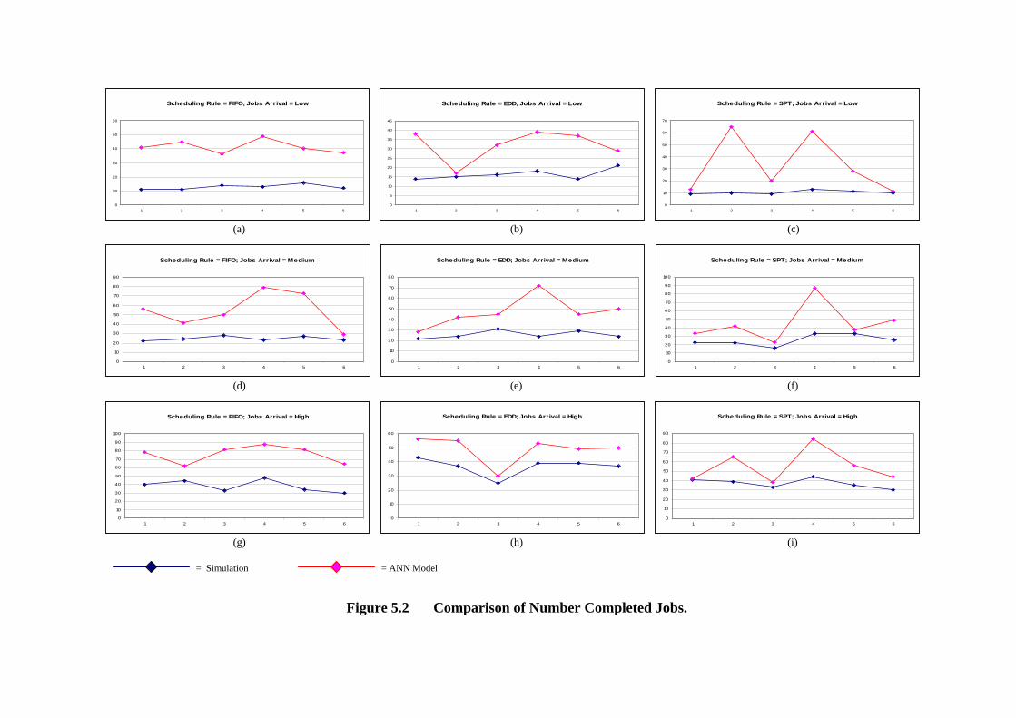
Scheduling Rule = FIFO; Jobs Arrival = Low

0

10

20

30

40

50

60

1 2 3 4 5 6

Scheduling Rule = EDD; Jobs Arrival = Low

0

5

10

15

20

25

30

35

40

45

1 2 3 4 5 6

Scheduling Rule = SPT; Jobs Arrival = Low

0

10

20

30

40

50

60

70

1 2 3 4 5 6 (a) (b) (c)

Scheduling Rule = FIFO; Jobs Arrival = Medium

0

10

20

30

40

50

60

70

80

90

1 2 3 4 5 6

Scheduling Rule = EDD; Jobs Arrival = Medium

0

10

20

30

40

50

60

70

80

1 2 3 4 5 6

Scheduling Rule = SPT; Jobs Arrival = Medium

0

10

20

30

40

50

60

70

80

90

100

1 2 3 4 5 6 (d) (e) (f)

Scheduling Rule = FIFO; Jobs Arrival = High

0

10

20

30

40

50

60

70

80

90

100

1 2 3 4 5 6

Scheduling Rule = EDD; Jobs Arrival = High

0

10

20

30

40

50

60

1 2 3 4 5 6

Scheduling Rule = SPT; Jobs Arrival = High

0

10

20

30

40

50

60

70

80

90

1 2 3 4 5 6 (g) (h) (i)

Figure 5.2 Comparison of Number Completed Jobs.

= Simulation = ANN Model

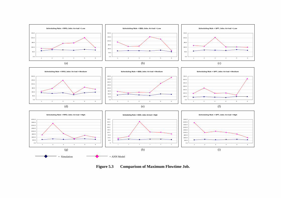
Scheduling Rule = FIFO; Jobs Arrival = Low

0.0

50.0

100.0

150.0

200.0

250.0

1 2 3 4 5 6

Scheduling Rule = EDD; Jobs Arrival = Low

0.0

50.0

100.0

150.0

200.0

250.0

300.0

1 2 3 4 5 6

Scheduling Rule = SPT; Jobs Arrival = Low

0.0

50.0

100.0

150.0

200.0

250.0

1 2 3 4 5 6 (a) (b) (c)

Scheduling Rule = FIFO; Jobs Arrival = Medium

0.0

50.0

100.0

150.0

200.0

250.0

300.0

1 2 3 4 5 6

Scheduling Rule = EDD; Jobs Arrival = Medium

0.0

50.0

100.0

150.0

200.0

250.0

300.0

350.0

400.0

1 2 3 4 5 6

Scheduling Rule = SPT; Jobs Arrival = Medium

0.0

100.0

200.0

300.0

400.0

500.0

600.0

700.0

1 2 3 4 5 6 (d) (e) (f)

Scheduling Rule = FIFO; Jobs Arrival = High

0.0

500.0

1000.0

1500.0

2000.0

2500.0

3000.0

3500.0

4000.0

1 2 3 4 5 6

Scheduling Rule = SPT; Jobs Arrival = High

0.0

500.0

1000.0

1500.0

2000.0

2500.0

3000.0

3500.0

4000.0

4500.0

1 2 3 4 5 6

(g) (h) (i)

Figure 5.3 Comparison of Maximum Flowtime Job.

Scheduling Rule = EDD; Jobs Arrival = High

0.0

500.0

1000.0

1500.0

2000.0

2500.0

3000.0

3500.0

4000.0

4500.0

1 2 3 4 5 6

= Simulation = ANN Model

Scheduling Rule = FIFO; Jobs Arrival = Low

0.000

0.200

0.400

0.600

0.800

1.000

1.200

1.400

1 2 3 4 5 6

Scheduling Rule = EDD; Jobs Arrival = Low

0.000

0.200

0.400

0.600

0.800

1.000

1.200

1 2 3 4 5 6

Scheduling Rule = SPT; Jobs Arrival = Low

0.000

0.200

0.400

0.600

0.800

1.000

1.200

1 2 3 4 5 6 (a) (b) (c)

Scheduling Rule = FIFO; Jobs Arrival = Medium

0.000

0.200

0.400

0.600

0.800

1.000

1.200

1.400

1.600

1.800

2.000

1 2 3 4 5 6

Scheduling Rule = EDD; Jobs Arrival = Medium

0.000

0.200

0.400

0.600

0.800

1.000

1.200

1.400

1.600

1.800

1 2 3 4 5 6

Scheduling Rule = SPT; Jobs Arrival = Medium

0.000

0.200

0.400

0.600

0.800

1.000

1.200

1.400

1 2 3 4 5 6 (d) (e) (f)

Scheduling Rule = FIFO; Jobs Arrival = High

0.000

0.500

1.000

1.500

2.000

2.500

3.000

1 2 3 4 5 6

Scheduling Rule = EDD; Jobs Arrival = High

0.000

0.200

0.400

0.600

0.800

1.000

1.200

1.400

1.600

1 2 3 4 5 6

Scheduling Rule = SPT; Jobs Arrival = High

0.000

0.200

0.400

0.600

0.800

1.000

1.200

1.400

1.600

1.800

1 2 3 4 5 6

(g) (h) (i)

Figure 5.4 Comparison of Average Machine Utilization.

= Simulation = ANN Model

Scheduling Rule = FIFO; Jobs Arrival = Low

0.000

0.050

0.100

0.150

0.200

0.250

0.300

1 2 3 4 5 6

Scheduling Rule = SPT; Jobs Arrival = Low

0.000

0.050

0.100

0.150

0.200

0.250

0.300

1 2 3 4 5 6

Scheduling Rule = EDD; Jobs Arrival = Low

0.000

0.050

0.100

0.150

0.200

0.250

0.300

1 2 3 4 5 6 (a) (b) (c)

Scheduling Rule = FIFO; Jobs Arrival = Medium

0.000

0.100

0.200

0.300

0.400

0.500

0.600

0.700

0.800

1 2 3 4 5 6

Scheduling Rule = EDD; Jobs Arrival = Medium

0.000

0.200

0.400

0.600

0.800

1.000

1.200

1.400

1.600

1 2 3 4 5 6

Scheduling Rule = SPT; Jobs Arrival = Medium

0.000

0.100

0.200

0.300

0.400

0.500

0.600

0.700

1 2 3 4 5 6 (d) (e) (f)

Scheduling Rule = FIFO; Jobs Arrival = High

0.000

20.000

40.000

60.000

80.000

100.000

120.000

140.000

1 2 3 4 5 6

Scheduling Rule = EDD; Jobs Arrival = High

0.000

20.000

40.000

60.000

80.000

100.000

120.000

1 2 3 4 5 6

Scheduling Rule = SPT; Jobs Arrival = High

0.000

10.000

20.000

30.000

40.000

50.000

60.000

70.000

80.000

90.000

100.000

1 2 3 4 5 6

(g) (h) (i)

Figure 5.5 Comparison of Average Job Q Length for the Machine.

= Simulation = ANN Model

64

65

66

67

68

69

70

71

72

73

74

75

76

77

78

79

80

81

82

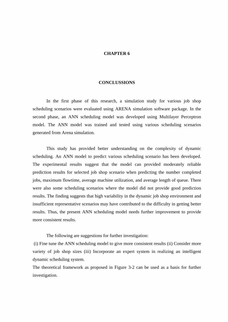
CHAPTER 6

CONCLUSSIONS

In the first phase of this research, a simulation study for various job shop

scheduling scenarios were evaluated using ARENA simulation software package. In the

second phase, an ANN scheduling model was developed using Multilayer Perceptron

model. The ANN model was trained and tested using various scheduling scenarios

generated from Arena simulation.

This study has provided better understanding on the complexity of dynamic

scheduling. An ANN model to predict various scheduling scenario has been developed.

The experimental results suggest that the model can provided moderately reliable

prediction results for selected job shop scenario when predicting the number completed

jobs, maximum flowtime, average machine utilization, and average length of queue. There

were also some scheduling scenarios where the model did not provide good prediction

results. The finding suggests that high variability in the dynamic job shop environment and

insufficient representative scenarios may have contributed to the difficulty in getting better

results. Thus, the present ANN scheduling model needs further improvement to provide

more consistent results.

The following are suggestions for further investigation:

(i) Fine tune the ANN scheduling model to give more consistent results (ii) Consider more

variety of job shop sizes (iii) Incorporate an expert system in realizing an intelligent

dynamic scheduling system.

The theoretical framework as proposed in Figure 3-2 can be used as a basis for further

investigation.

LIST OF REFERENCES

Abumaizar, R. J., and Svestka, J. A., 1997. Rescheduling job shops under disruptions. International Journal of Production Research, 35, 2065-2082.

Azizoğlu M. and Alagoz, O, (2003), Rescheduling of identical parallel machines under machine eligibility constraints, European Journal of Operational Research, Vol. 149, pp. 523–532

Azizoğlu M. and Alagoz, O, (2002), Parallel machine rescheduling with machine disruptions, Middle East Technical University, Department of Industrial Engineering, Turkey, pp. 1-20

Baker, K. R. (1984), Sequencing rules and due-dates assignment in a job-shop, Management Science, Vol. 30: pp. 1093-1104.

Baker K. R. (1974), Introduction to Sequencing and Scheduling. New York: John Willey & Sons.

Balasubramanian, J., and Grossmann, I. E. (2002), A novel branch and bound algorithm for scheduling flowshop plants with uncertain processing times, Computers and Chemical Engineering. Vol. 26: pp. 41–57.

Banks, J. (1998), Handbook of Simulation, New York: John Willey and Sons, Inc..

Bean, James C., John R. Birge, John Mittenthal, and Charles E. Noon, “Matchup scheduling with multiple resources, release dates, and disruptions,” Operations Research, Volume 39, Number 3, pages 470-483, 1991.

Belz, R., and Martens, P., (1996), Combining knowledge-based system and simulation to solve resceduling problems, Decision Support Systems, Vol. 17: pp. 141-157

Benjaafar, S. and Sheikhzadeh, M. (1997), Scheduling policies, batch sizes, and manufacturing lead times. IEE Transaction, Vol. 29: pp. 159-166

Bilkay O. Anlagan, O., and Kilic, S. E., (2004), Job shop scheduling using fuzzy logic, Int J Adv Manuf Technol. Vol. 23, pp. 606–619

85

Black, J.T., (1983), Manufacturing systems, Kluwer, Norwell, Massachusetts.

Blazewicz, J., Domschke, W., and Pesch, E. (1996), The Job Shop Scheduling Problem: Conventional and New Techniques, European Journal of Operation Research. Vol. 93: pp. 1-33.

Blazewicz, J. et al. (1993), Scheduling in Computer and Manufacturing Systems, Springer-Verlag,

Brizuela, C.A., and Sannomiya, N., (1999), From the classical Job Shop to a real Problem: A Genetic Algorithm Approach. Kyoto Institute of technology, Japan.

Brucker, P. (1995), Scheduling Algorithm, New York: Springer Verlag.

Buxey, G. (1989), Production Scheduling: Practice and theory, European Journal of Operation Research, Vol. 39: pp. 17-31.

Cave, A., Nahavandi, S., and Kouzani, A., (2002), Simulation Optimization for Process Scheduling Trough Simulated Annealing, Proceedings of the 2002 Winter Simulation Conference

Chang, F. C. R. (1996), A study of due-date assignment rules with constrained tightness in a dynamic job shop, Discrete Applied Mathematics, Vol. 77: pp. 185-200.

Cheng, R., et al. (1996), A bi-criteria optimization - minimizing the integral value and spread of the fuzzy makespan of job shop scheduling problems, Computers ind. Engng, Vol. 30(4): pp. 983-997.

Cheng, T. C. E. and Kovalov, M. Y. (2001), Single Machine batch Scheduling with Sequential Job Processing. IEE Transaction, Vol. 33: pp. 413-420.

Cheng, T. C. E., Liu Z., and Wenci, (2001), Scheduling jobs with release dates and deadlines on batch processing machine, IEE Transaction. Vol. 33: pp. 685-690.

Chong, C. S., Sivakumar, A. I. and Gay, R. (2003) Simulation Based Scheduling for Dynamic Discrete Manufacturing, Proceeding of the 2003 Winter Simulation Conference, pp. 1465-1473

Church, L.K., Uzsoy, R., (1992). Analysis of periodic and event driven rescheduling policies in dynamic shops. International Journal of Computer Integrated Manufacturing Vol. 5 (3), pp. 153-163.

86

Chryssolouris G. (1992), Manufacturing Systems. Theory and Practice, New York: Springer-Verlag.

Conway, R., Maxwell, W., and Miller, L. (1967), Theory of Scheduling, Addison-Wesley, Publishing Company.

Cottet, F., Kaiser, J. D. C., and Mammeri, Z., (2002), Scheduling in Real-Time System, Chichester, England: John Wiley & Son, Ltd.

Chun, H. W. and Wong, R. Y. M., 2003, an agent-based negotiation algorithm for dynamic scheduling and rescheduling, Advanced Engineering Informatics, Vol. 17, pp. 1-22

Dhingra, J. S., Musser, K. L., and Blankenship, G. L., 1992. Real-time operations scheduling for flexible manufacturing systems. Proceeding of the 1992 Winter Simulation Conference, 849-855.

Diaz, A. R., Tchernykh,A., and Ecker,K. H., 2003, Algorithms for dynamic scheduling of unit execution time tasks, European Journal of Operational Research 146, pp. 403–416

Dominic, P. D. D., and Kaliyamoorty, S. (2004), Efficient Dispatching Rules for Dynamic Job Shop Scheduling, Journal of Manufacturing Technology. Vol. 24: pp. 70-75.

Drexl, A. (1997), Lot Sizing and Scheduling, - Survey and Extension, European Journal of Operation Research, Vol. 99, 1997, pp. 271-235.

Dunstall, S. and Wirth, A. (2001), Models and Algorithms for Machine Scheduling with setup Times. Elvers, D. A., and Taube (1988), L. R., Time completion of various dispatching rules in job shop, OMEGA. Vol. 11: pp. 81-89.

Elvers, D.A. and Taube, L.R., (1983), Time completion for various dispatching rules in job shops, Omega, Vol. II (1), pp. 81-9.

El-Bouri, A., Balakrishnan, S., , and Popplewell, N., (2000), Sequencing jobs on a single machine: A neural network approach, European Journal of Operational Research, Vol. 126, pp. 474-490.

Emery, J. C. (1969), Job Shop Scheduling by Mean Simulation and an Optimum-Seeking Search, University of Pennsylvania, Philadelphia, Pennsylvania: pp. 363-372.

Fang, J., and Xi, Y., 1997. A rolling horizon job shop rescheduling strategy in the dynamic environment. The International Journal of Advanced Manufacturing Technology, 13, 227-232

87

Fonseca, D. J., and Navaresse, D. (2002), Artificial neural networks for job shop simulation, Engineering Informatics, Vol. 16: pp. 241-246.

French, S., (1982), Scheduling and Sequencing, Chicherster, London: John Willey & Sons (Ellis Horwood Ltd),

Fry, D., Phillipoom, P.R., and Blackstone, J. H. (1988), A simulation study of processing time dispatching rules, Journal of Operation Management. Vol. 7: pp. 77-92.

Graves S. C. (1981), A Review of Production Scheduling, Operation Research, Vol. 29: pp. 647-675.

Guh, R-S., 2004, Optimizing Feed forward Neural Network for Control Chart Pattern Recognition Through Genetic Algorithms, International Journal of Pattern Recognition and Artificial Intelligent. Vol. 18(2), pp. 75-99.

Gupta, S. K. (1981), Production Scheduling Techniques. K. P. Bagchi & Company

Hassan, A, (2002), On-line recognition of developing control chart pattern, PhD dissertation, University Teknologi Malaysia.

Hall, N. G. (1996), A Survey of Machine Scheduling Problems with Blocking and No-wait in Process. Operation Research, Vol. 44: pp. 510-525.

Heywood, M. I., Chan, M.C., and Chatwin C. R., (1997), Aplication of stochastic real valued reinforcement neural network to batch production rescheduling, Proceedings of the Institution of Mechanical Engineers, , 211, , 591-603

Hoitomt, D. J., and Luh, P. B. (1993), Scheduling the Dynamic Job Shop. IEEE. pp. 71-76.

Holloway, C.A., and Nelson, R.T., (1974). Job shop scheduling with due dates and variable processing times. Management Science, Vol. 20 (9), pp. 65-75.

Holthaus, O. (1999), Scheduling in job shops with machine breakdowns - an experimental study, Computers & Industrial Engineering. Vol. 36: pp. 137-162.

Jackson J. R. (1963), Jobshop-like queueing system, Managemnet science, Vol. 10: pp. 518-521.

Jain, A. K., and Elmaraghy, H. A., 1997. Production scheduling/rescheduling in flexible manufacturing. International Journal of Production Research, 35, 281-309.

88

Jang, W., (2002), Dynamic scheduling of stochastic jobs on a single machine, European Journal of Operational Research, Vol. 138: pp. 518–530.

Jensen, M. T. (2001), Improving robustness and flexibility of tardiness and total flow-time job shops using robustness measures, Applied Soft Computing, Vol. 1: pp. 35–52.

Jensen, J. (1999) Introduction to Computer Simulation and the Simulation Process, A Guide to Business Decision-Making Using Visual SLAM II and AweSim

Jordan, C. (1996), Batching and Scheduling, Springer.

Kacem, I.., Hammadi, S., and Borne P. (2002), Pareto-optimality approaches for flexible job-shop scheduling problems - hybridization of evolutionary algorithms and fuzzy logic. Mathematics and Computers in Simulation, Vol. 60: pp. 245-276.

Kamaruddin, S. and Duffill, A. W. (2001), Dynamic Scheduling - a knowledge-based system (KBS) approach, Proceeding of the Seventeenth National Confrence on Manufacturing Research, pp 287-292

Karatza, Helen D. (2000), A Comparative of Scheduling Policies in a Distributed system Using Simulation, International Journal of Simulation, Vol. 1(1-2): pp. 12-20.

Kempf, Karl G., “Intelligently scheduling semiconductor wafer fabrication,” in Intelligent Scheduling, M. Zweben and M.S. Fox, eds., Morgan Kaufmann Publishers, San Francisco, 1994.

Kim and Kim, 1994, Simulation based real time scheduling in a flexible manufacturing system, Journal of Manufacturing System, Vol. 13(2), pp. 85-93.

Kimms, A. (1997), Multi-level Lot Sizing and Scheduling, ,Physica-Verlag.

Kiran, A. S., and Smith, M. L. (1984), Simulation studies in Job Shop Scheduling – I A Survey. Computing & Industrial Engineering, Vol. 8: pp. 87-93.

Kiran, A. S., and Smith, M. L. (1984), Simulation studies in Job Shop Scheduling – II Performance of priority rules. Computing & Industrial Engineering, Vol. 8: pp. 95-105.

Kumar, P.R., “Scheduling manufacturing systems of re-entrant lines,” in Stochastic Modeling and Analysis of Manufacturing Systems, David D. Yao, ed., pages 325-360, Springer-Verlag, New York, 1994

89

Kuroda, M. and Wang Z. (1996), Fuzzy job shop scheduling. Int. J. Production Economics, Vol. 44: pp. 45-51.

Lee, C. Y., Lei, L. and Pinedo, M. (1997), Current trends in deterministic scheduling, Annals of Operations Research, Vol. 70: pp. 1– 41.

Lee, I., and Shaw, M. J. (2000), A neural-net approach to real time flow-shop sequencing, Computers & Industrial Engineering, Vol. 38: pp. 125-147.

Lengyel, A., Hatono, I., and Ueda K., (2003), Scheduling for on-time completion in job shops using feasibility function, Computers & Industrial Engineering, Vol. 45: pp. 215-229.

Li, et. al. (2000), A production rescheduling expert simulation system. European Journal of Operational Research, Vol. 124: pp. 283-293.

Li, Y. C. E., Shaw, Jr. and Martin-Vega, L-A., (1996), Flow-time Performance of Modified Scheduling Heuristics in a Dynamic Rescheduling Environment, Computers ind. Engng, Vol. 31(1/2), 213-216

Li, Y. C. E. and Wade H. Shaw, (1998), Simulation modeling of a dynamic job shop rescheduling with machine availability constraints, Computers ind. Engng, Vol., 35(1-2), . pp. 117-120.

Liu, S.Q. , Ong, H.L. and Ng, H.L. (2005), Metaheuristics for minimizing the makespan of the dynamic shop scheduling problem, Advances in Engineering Software, Vol. 36, pp. 199–205

Luh, Peter B., Chen, Dong, and Thakur, Lakshman S. (1999), An Effective Approach for Job-Shop Scheduling with Uncertain Processing Requirements, IEEE Transactions on Robotics and Automation, Vol.15(2): pp. 328-339.

Madureira, A. and Ramos, C., (2001), A New Framework for Deterministic Job-shop Scheduling problems Using Genetic Algorithms, Dept. de Engenharia Informatica, Instituto Superior de Engenharia do Porto, Protugal.

Maturana, F. et al. (1997), Object-oriented job-shop scheduling using genetic algorithms, Computers in Industry, Vol. 32: pp. 281-294.

Mehta, A. (2000) Smart Modeling-Basic Methodology and Advanced Tools, Proceeding of the 2000 Winter Simulation Conference: pp. 241-245.

Mokotoff, E. (2001), Parallel Machine Scheduling Problems: A Survey, Asia-Pacific Journal of Operation Research, Vol. 18: pp. 193-242.

90

Muhleman, A.P., Lockett, A.G., Farn, C.K., (1982). Job shopscheduling heuristics and frequency of scheduling. International Journal of Production Research. Vol. 20 (2), pp. 227-241.

Nagar, A., Haddock, J. and Heragu, S. (1995), Multiple and Bicriteria Scheduling: A Literature Survey, European Journal of Operation Research, Vol. 81: pp. 88-104.

Olumolade, M. O., and Norrie, D. H., 1996. Reactive scheduling system for cellular manufacturing with failure-prone machines. International Journal of Computer Integrated Manufacturing., 9, 2, 131-144.

Panwalker, S.S., (1977). A survey of scheduling rules. Operations Research 25, 45–61.

Pendharkar, P.C., (1999), A computational study on design and performance issues of multi-agent intelligent systems for dynamic scheduling environments, Expert Systems with Applications, Vol. 16. pp. 121–133.

Parka, Y., Kima, S., and Lee, Y-H. (2000), Jobs on parallel machines applying neural network and heuristic rules, Computers & Industrial Engineering, Vol. 38: pp. 189-202.

Pichitlamken, J., and Nelson, B. L. (2001), Selection-of-the-Best Procedures for Optimization via Simulation, Proceeding of the 2001 Winter Simulation Conference: pp. 401-407.

Pinedo, M. (2002), Scheduling: Theory, Algorithm, and System, 2nd. Ed. Englewood Cliffs, New Jersey. Prentice Hall,

Raheja, A. S., and Subramaniam, V. (2002), Reactive Recovery of Job Shop Schedules – A Survey. The International Journal of Advanced Manufacturing Technology, Vol. 19: pp. 756-763.

Ramashes, R. (1990) Dynamic Job Shop Scheduling: A Survey of Simulation Research. OMEGA, Vol. 18: pp. 43-57.

Rangsaritratsameea,R., Ferrell, W. G.Jr., and Kurz, M. B., 2004, Dynamic rescheduling that simultaneously considers efficiency and stability, Computers & Industrial Engineering, Vol. 46, pp. 1-15

Rardin, R. E., (1998), Optimization in Operation Research, New Jersey: Prentice Hall,

Rinooy Kan, A. H. G. (1979), Machine Scheduling Problems: Classification, Complexity and Computation. Martinus Nijhoff, The Hague.

91

Sabuncuoglu, I. and Karabuk,S., (1999), Rescheduling Frequency in an FMS with Uncertain Processing Times and Unreliable Machines, Journal of Mfg. Systems, Vol . 18(4), pp. 268-283.

Sabuncuoglu, I., and Gurgun, B., (1996), A neural network model for scheduling problems, European Journal of Operational Research, Vol. 93 , pp. 288-299.

Sabuncuoglu, I. and Bayõz,M. (2000), Analysis of reactive scheduling problems in a job shop environment. European Journal of Operational Research, Vol. 126: pp. 567-586.

Sadeh, N., and Fox, M. S. (1996), Variable and value ordering heuristics for the job shop scheduling constraint satisfaction problem. Artificial Intelligence, pp. 86

Sen, T., and Gupta, S. K. (1984), A state-of-the-art survey of static scheduling research involving due dates, OMEGA, Vol. 12: pp 63-76.

Schmidt, J. W. (1986), Introduction to System Analysis, Modeling and Simulation, Proceedings of the 1986 Winter Simulation Conference: pp. 5-16.Sevastjanov, S. V. (1994), On Some Geometric Method in Scheduling Theory: A Survey. Discrete Applied Mathematics, Vol. 55: pp. 59-82.

Shafaei, R., and Brunn, P., 1999. Workshop scheduling using practical (inaccurate) data - Part 1: The performance of heuristic scheduling rules in a dynamic job shop environment using a rolling time horizon approach. International Journal of Production Research, 37, 17, 3913-3925.

Sivazlian, B. D. (1975), Optimization Techniques in Operation Research. Englewood Cliff, New Jersey: Prentice Hall, Inc.

Song, D. P., Hicks, C. and Earl, C. F., 2001, Dynamic production scheduling and rescheduling for complex assemblies, Dept. of Earth science and engineering, royal school of mines, UK, pp. 1-16

Sursesh, V., and Chauduri, D. (1993), Dynamic Scheduling – A survey of research, International Journal of Production Economics, Vol. 32: pp. 53-66.

Sun, J., and Xue, D., 2001, A dynamic reactive scheduling mechanism for responding to changes of poduction orders and manufacturing resources, Computers in Industry, Vol. 46, pp. 189-207

V. Subramaniam, T. Ramesh, G. K. Lee, Y. S. Wong and G. S. Hong, (2000) Job Shop Scheduling with Dynamic Fuzzy Selection of Dispatching Rules, In.t J Adv Manufacturing Technology. Vol. 16, pp.759–764.

92

Vieira G. E., Herrmann, J. W., and Lin, E., (2000), Predicting the Performance of Rescheduling Strategies for Parallel Machine Systems, Journal of Manufacturing Systems, Vol. 19(4),pp. 256-266.

Vieira G. E., Herrmann, J. W., and Lin, E., (2001), Rescheduling manufacturing systems: a framework of strategies, policies, and methods, Department of Mechanical Engineering University of Maryland, pp. 1-39

Watanabe, T., Tokumaru, H., and Hashimoto, Y., (2003), Job-shop scheduling using neural networks, Department of Computer Science and Systems Engineering, Ritsumeikan University, Kyoto 603-77, Japan

Watatani, Y., and Fujii, S., 1992. A study on rescheduling policy in production system. JAPAN/USA Symposium on Flexible Automation, Vol.2, ASME.

Weeks, J. K., and Fryer, J. S. (1976), A simulation study of operating policies in a hypothetical dual-constrained job shop. Management Science, Vol. 22: pp. 1362-1370.

Wu, S. D., Storer, R. H., and Chang, P. -C., 1993. One-machine rescheduling heuristics with efficiency and stability as criteria. Computers & Operations Research, 20, 1-14.

Yamamoto, M., Nof, S.Y., 1985. Scheduling in the manufacturing operating system environment. International Journal of Production Research, Vol. 23 (4), pp. 705-722.

Yang, S. and Wang D. (2001), A new adaptive neural network and heuristics hybrid approach for job-shop scheduling, Computers & Operations Research, Vol. 28: pp. 955-971.

Ying, C. C. (1996), Specification of a job shop scheduling simulation model and some properties of its internal transition function, Computers & Industrial Engineering, Vol. 31(1-2): pp. 201-204.

Yu, H., and Liang, W., (2001), Neural Network and Genetic Algorithm-based hybrid approach to expanded job-shop scheduling, Computer & industrial Engineering, Vol. 39, pp. 337-356

APPENDIX A Most Common Scheduling Rules

1. Job Scheduling Rules EDD Earliest Due Dates EDF Earliest Deadline First FASFO First At Shop First Out FCFS First Come First Served FIFO First In First Out FRO Fewest number of Remaining Opertion LDT Longest SIO/TP ratio LIO Longest Imminent Operation time LLF Least Laxity First (Laxity =kelemahan) LMT Longest SIO.TP Multiplication Time LPT Longest Processing Time LRPT Longest Remaining Processing Time MRO Largest number of Remaining Opertion SDT Shortest SIO/TP ratio SIO Shortest Imminent Operation time (Imminent = hampir sampai

gilirannya) SMT Shortes SIO.TP Multiplication Time SPT Shortest Processing Time SRPT Shortest Remaining Processing Time

2. Machine Scheduling Rules FAFS First Arrived First Served FCFS First Come First Served FOPNR Fewest number of operation remaining LPT. TOT Largest value of operation time multiplied by total operation time LPT/TOT Largest value of operation time divided by total operation time LWKR Least work remaining MOPNR Most number of operation remaining MWKR Most work remaining RANDOM Job priority is random SPT Shortest Processing Time SPT. TOT Smallest value of operation time multiplied by total operation

time SPT/TOT Smallest value of operation time divided by total operation time

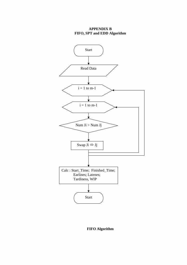
APPENDIX B FIFO, SPT and EDD Algorithm

FIFO Algorithm

Read Data

Num Ji > Num Jj

Swap Ji Jj

Start

i = 1 to m-1

i = 1 to m-1

Calc : Start_Time; Finished_Time; Earlines; Latenes; Tardiness, WIP

Start

95

SPT Algorithm

Read Data

Pt Ji > Due date Pt Jj

Swap Ji Jj

Start

i = 1 to m-1

i = 1 to m-1

Calc : Start_Time; Finished_Time; Earlines; Latenes; Tardiness, WIP

Start

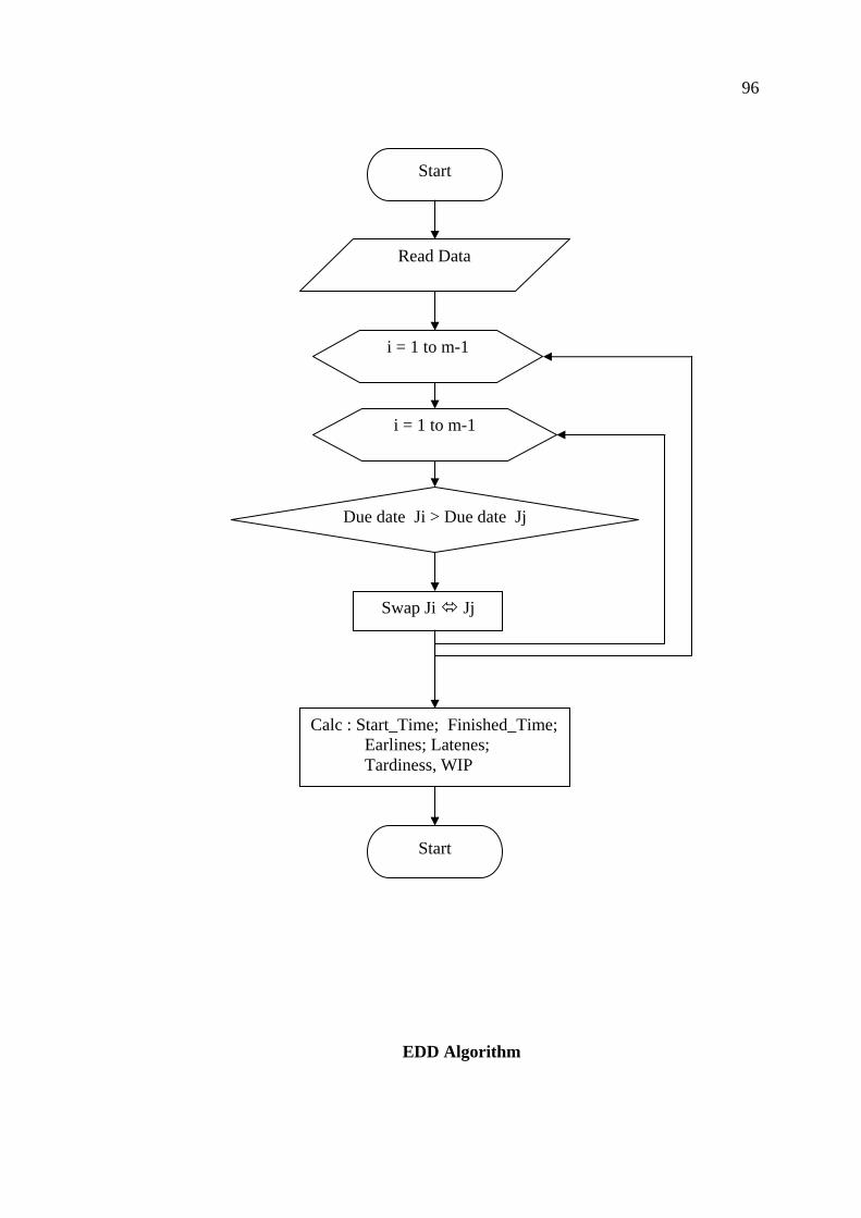
96

EDD Algorithm

Read Data

Due date Ji > Due date Jj

Swap Ji Jj

Start

i = 1 to m-1

i = 1 to m-1

Calc : Start_Time; Finished_Time; Earlines; Latenes; Tardiness, WIP

Start

Appendix C

Most Common Performance Measure

1. Time-based measure

Mean and variance of flow time per job

Mean and variance of flow time per operation

Mean waiting time

Mean idle time 2. WIP Measure

Average number of job in queue

Average number of operation in queue

Value of work-in-process 3. Due-date related measure

Mean tardiness

Conditional mean tardiness

Proportional of job tardy

Mean lateness

Number of job tardy

Maximum lateness 4. Cost-based Measure

Cost of idle machines

Cost of long promises

Cost of carrying work-in-process

Total cost per job

Average value added in queue

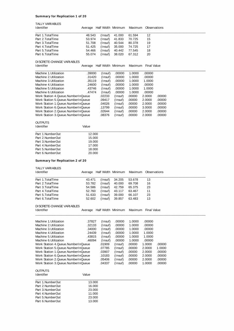
Summary for Replication 1 of 20 TALLY VARIABLES Identifier Average Half Width Minimum Maximum Observations ___________________________________________________________________________________________________ Part 1.TotalTime 48.543 (Insuf) 41.000 61.594 12 Part 2.TotalTime 53.974 (Insuf) 41.833 70.725 15 Part 3.TotalTime 51.708 (Insuf) 40.544 80.378 19 Part 4.TotalTime 51.425 (Insuf) 35.000 74.725 17 Part 5.TotalTime 54.466 (Insuf) 40.442 77.545 18 Part 6.TotalTime 55.074 (Insuf) 38.020 67.312 20 DISCRETE-CHANGE VARIABLES Identifier Average Half Width Minimum Maximum Final Value ___________________________________________________________________________________________________ Machine 1.Utilization .39000 (Insuf) .00000 1.0000 .00000 Machine 2.Utilization .31420 (Insuf) .00000 1.0000 .00000 Machine 3.Utilization .35119 (Insuf) .00000 1.0000 1.0000 Machine 4.Utilization .24600 (Insuf) .00000 1.0000 .00000 Machine 5.Utilization .43746 (Insuf) .00000 1.0000 1.0000 Machine 6.Utilization .47474 (Insuf) .00000 1.0000 .00000 Work Station 4.Queue.NumberInQueue .02233 (Insuf) .00000 2.0000 .00000 Work Station 5.Queue.NumberInQueue .09417 (Insuf) .00000 2.0000 .00000 Work Station 1.Queue.NumberInQueue .04026 (Insuf) .00000 2.0000 .00000 Work Station 6.Queue.NumberInQueue .13799 (Insuf) .00000 3.0000 .00000 Work Station 2.Queue.NumberInQueue .02644 (Insuf) .00000 2.0000 .00000 Work Station 3.Queue.NumberInQueue .08376 (Insuf) .00000 2.0000 .00000 OUTPUTS Identifier Value _____________________________________________________________ Part 1.NumberOut 12.000 Part 2.NumberOut 15.000 Part 3.NumberOut 19.000 Part 4.NumberOut 17.000 Part 5.NumberOut 18.000 Part 6.NumberOut 20.000 Summary for Replication 2 of 20 TALLY VARIABLES Identifier Average Half Width Minimum Maximum Observations ___________________________________________________________________________________________________ Part 1.TotalTime 43.471 (Insuf) 34.205 53.678 13 Part 2.TotalTime 53.782 (Insuf) 40.000 69.708 16 Part 3.TotalTime 54.586 (Insuf) 42.759 65.375 23 Part 4.TotalTime 52.760 (Insuf) 43.117 63.467 11 Part 5.TotalTime 51.633 (Insuf) 39.000 66.107 23 Part 6.TotalTime 52.602 (Insuf) 39.857 63.483 13 DISCRETE-CHANGE VARIABLES Identifier Average Half Width Minimum Maximum Final Value ___________________________________________________________________________________________________ Machine 1.Utilization .37827 (Insuf) .00000 1.0000 .00000 Machine 2.Utilization .32133 (Insuf) .00000 1.0000 .00000 Machine 3.Utilization .34000 (Insuf) .00000 1.0000 .00000 Machine 4.Utilization .24439 (Insuf) .00000 1.0000 1.0000 Machine 5.Utilization .43815 (Insuf) .00000 1.0000 1.0000 Machine 6.Utilization .46094 (Insuf) .00000 1.0000 .00000 Work Station 4.Queue.NumberInQueue .01909 (Insuf) .00000 1.0000 .00000 Work Station 5.Queue.NumberInQueue .07785 (Insuf) .00000 2.0000 1.0000 Work Station 1.Queue.NumberInQueue .03907 (Insuf) .00000 2.0000 .00000 Work Station 6.Queue.NumberInQueue .10183 (Insuf) .00000 2.0000 .00000 Work Station 2.Queue.NumberInQueue .05406 (Insuf) .00000 2.0000 .00000 Work Station 3.Queue.NumberInQueue .04337 (Insuf) .00000 1.0000 .00000 OUTPUTS Identifier Value _____________________________________________________________ Part 1.NumberOut 13.000 Part 2.NumberOut 16.000 Part 3.NumberOut 23.000 Part 4.NumberOut 11.000 Part 5.NumberOut 23.000 Part 6.NumberOut 13.000

99Summary for Replication 3 of 20 TALLY VARIABLES Identifier Average Half Width Minimum Maximum Observations ___________________________________________________________________________________________________ Part 1.TotalTime 42.292 (Insuf) 35.602 51.704 13 Part 2.TotalTime 54.754 (Insuf) 41.869 73.876 19 Part 3.TotalTime 54.178 (Insuf) 42.000 70.109 12 Part 4.TotalTime 55.466 (Insuf) 38.000 71.103 15 Part 5.TotalTime 54.972 (Insuf) 41.724 76.140 23 Part 6.TotalTime 56.155 (Insuf) 45.179 70.805 18 DISCRETE-CHANGE VARIABLES Identifier Average Half Width Minimum Maximum Final Value ___________________________________________________________________________________________________ Machine 1.Utilization .40533 (Insuf) .00000 1.0000 .00000 Machine 2.Utilization .34263 (Insuf) .00000 1.0000 1.0000 Machine 3.Utilization .35032 (Insuf) .00000 1.0000 .00000 Machine 4.Utilization .22667 (Insuf) .00000 1.0000 .00000 Machine 5.Utilization .43733 (Insuf) .00000 1.0000 .00000 Machine 6.Utilization .49555 (Insuf) .00000 1.0000 .00000 Work Station 4.Queue.NumberInQueue .01163 (Insuf) .00000 1.0000 .00000 Work Station 5.Queue.NumberInQueue .08179 (Insuf) .00000 2.0000 .00000 Work Station 1.Queue.NumberInQueue .03500 (Insuf) .00000 2.0000 .00000 Work Station 6.Queue.NumberInQueue .14589 (Insuf) .00000 3.0000 .00000 Work Station 2.Queue.NumberInQueue .03024 (Insuf) .00000 1.0000 .00000 Work Station 3.Queue.NumberInQueue .08460 (Insuf) .00000 2.0000 .00000 OUTPUTS Identifier Value _____________________________________________________________ Part 1.NumberOut 13.000 Part 2.NumberOut 19.000 Part 3.NumberOut 12.000 Part 4.NumberOut 15.000 Part 5.NumberOut 23.000 Part 6.NumberOut 18.000 Summary for Replication 4 of 20 TALLY VARIABLES Identifier Average Half Width Minimum Maximum Observations ___________________________________________________________________________________________________ Part 1.TotalTime 42.149 (Insuf) 35.721 59.240 12 Part 2.TotalTime 56.313 (Insuf) 44.000 69.257 17 Part 3.TotalTime 54.428 (Insuf) 44.591 78.107 11 Part 4.TotalTime 49.989 (Insuf) 38.000 79.014 21 Part 5.TotalTime 52.022 (Insuf) 43.000 62.000 31 Part 6.TotalTime 47.344 (Insuf) 43.574 52.399 6 DISCRETE-CHANGE VARIABLES Identifier Average Half Width Minimum Maximum Final Value ___________________________________________________________________________________________________ Machine 1.Utilization .34354 (Insuf) .00000 1.0000 1.0000 Machine 2.Utilization .33200 (Insuf) .00000 1.0000 .00000 Machine 3.Utilization .38828 (Insuf) .00000 1.0000 .00000 Machine 4.Utilization .21989 (Insuf) .00000 1.0000 1.0000 Machine 5.Utilization .45486 (Insuf) .00000 1.0000 .00000 Machine 6.Utilization .43267 (Insuf) .00000 1.0000 .00000 Work Station 1.Queue.NumberInQueue .03092 (Insuf) .00000 2.0000 .00000 Work Station 2.Queue.NumberInQueue .03590 (Insuf) .00000 2.0000 .00000 Work Station 3.Queue.NumberInQueue .04288 (Insuf) .00000 1.0000 .00000 Work Station 4.Queue.NumberInQueue .01646 (Insuf) .00000 1.0000 1.0000 Work Station 5.Queue.NumberInQueue .08696 (Insuf) .00000 2.0000 .00000 Work Station 6.Queue.NumberInQueue .06718 (Insuf) .00000 2.0000 .00000 OUTPUTS Identifier Value _____________________________________________________________ Part 1.NumberOut 12.000 Part 2.NumberOut 17.000 Part 3.NumberOut 11.000 Part 4.NumberOut 21.000 Part 5.NumberOut 31.000 Part 6.NumberOut 6.0000

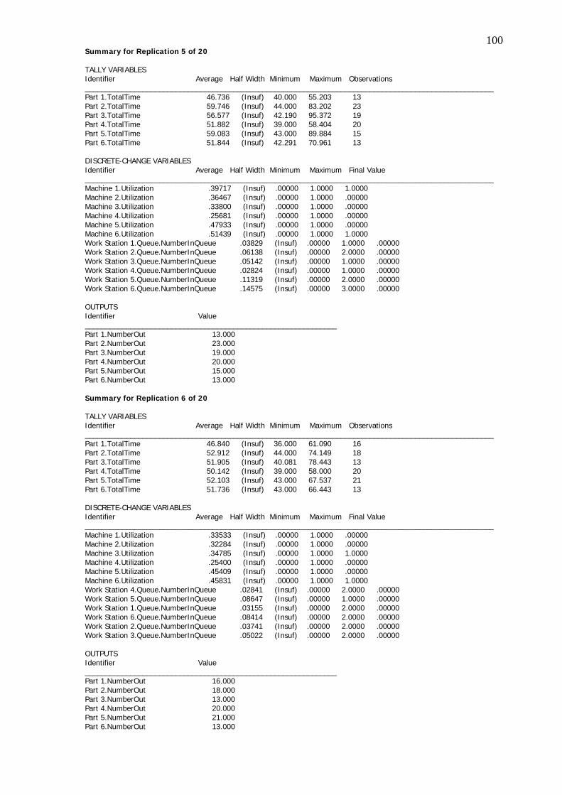
100Summary for Replication 5 of 20 TALLY VARIABLES Identifier Average Half Width Minimum Maximum Observations ___________________________________________________________________________________________________ Part 1.TotalTime 46.736 (Insuf) 40.000 55.203 13 Part 2.TotalTime 59.746 (Insuf) 44.000 83.202 23 Part 3.TotalTime 56.577 (Insuf) 42.190 95.372 19 Part 4.TotalTime 51.882 (Insuf) 39.000 58.404 20 Part 5.TotalTime 59.083 (Insuf) 43.000 89.884 15 Part 6.TotalTime 51.844 (Insuf) 42.291 70.961 13 DISCRETE-CHANGE VARIABLES Identifier Average Half Width Minimum Maximum Final Value ___________________________________________________________________________________________________ Machine 1.Utilization .39717 (Insuf) .00000 1.0000 1.0000 Machine 2.Utilization .36467 (Insuf) .00000 1.0000 .00000 Machine 3.Utilization .33800 (Insuf) .00000 1.0000 .00000 Machine 4.Utilization .25681 (Insuf) .00000 1.0000 .00000 Machine 5.Utilization .47933 (Insuf) .00000 1.0000 .00000 Machine 6.Utilization .51439 (Insuf) .00000 1.0000 1.0000 Work Station 1.Queue.NumberInQueue .03829 (Insuf) .00000 1.0000 .00000 Work Station 2.Queue.NumberInQueue .06138 (Insuf) .00000 2.0000 .00000 Work Station 3.Queue.NumberInQueue .05142 (Insuf) .00000 1.0000 .00000 Work Station 4.Queue.NumberInQueue .02824 (Insuf) .00000 1.0000 .00000 Work Station 5.Queue.NumberInQueue .11319 (Insuf) .00000 2.0000 .00000 Work Station 6.Queue.NumberInQueue .14575 (Insuf) .00000 3.0000 .00000 OUTPUTS Identifier Value _____________________________________________________________ Part 1.NumberOut 13.000 Part 2.NumberOut 23.000 Part 3.NumberOut 19.000 Part 4.NumberOut 20.000 Part 5.NumberOut 15.000 Part 6.NumberOut 13.000 Summary for Replication 6 of 20 TALLY VARIABLES Identifier Average Half Width Minimum Maximum Observations ___________________________________________________________________________________________________ Part 1.TotalTime 46.840 (Insuf) 36.000 61.090 16 Part 2.TotalTime 52.912 (Insuf) 44.000 74.149 18 Part 3.TotalTime 51.905 (Insuf) 40.081 78.443 13 Part 4.TotalTime 50.142 (Insuf) 39.000 58.000 20 Part 5.TotalTime 52.103 (Insuf) 43.000 67.537 21 Part 6.TotalTime 51.736 (Insuf) 43.000 66.443 13 DISCRETE-CHANGE VARIABLES Identifier Average Half Width Minimum Maximum Final Value ___________________________________________________________________________________________________ Machine 1.Utilization .33533 (Insuf) .00000 1.0000 .00000 Machine 2.Utilization .32284 (Insuf) .00000 1.0000 .00000 Machine 3.Utilization .34785 (Insuf) .00000 1.0000 1.0000 Machine 4.Utilization .25400 (Insuf) .00000 1.0000 .00000 Machine 5.Utilization .45409 (Insuf) .00000 1.0000 .00000 Machine 6.Utilization .45831 (Insuf) .00000 1.0000 1.0000 Work Station 4.Queue.NumberInQueue .02841 (Insuf) .00000 2.0000 .00000 Work Station 5.Queue.NumberInQueue .08647 (Insuf) .00000 1.0000 .00000 Work Station 1.Queue.NumberInQueue .03155 (Insuf) .00000 2.0000 .00000 Work Station 6.Queue.NumberInQueue .08414 (Insuf) .00000 2.0000 .00000 Work Station 2.Queue.NumberInQueue .03741 (Insuf) .00000 2.0000 .00000 Work Station 3.Queue.NumberInQueue .05022 (Insuf) .00000 2.0000 .00000 OUTPUTS Identifier Value _____________________________________________________________ Part 1.NumberOut 16.000 Part 2.NumberOut 18.000 Part 3.NumberOut 13.000 Part 4.NumberOut 20.000 Part 5.NumberOut 21.000 Part 6.NumberOut 13.000

101Summary for Replication 7 of 20 TALLY VARIABLES Identifier Average Half Width Minimum Maximum Observations ___________________________________________________________________________________________________ Part 1.TotalTime 43.443 (Insuf) 35.887 52.523 14 Part 2.TotalTime 57.134 (Insuf) 42.000 68.931 16 Part 3.TotalTime 55.495 (Insuf) 44.653 70.907 17 Part 4.TotalTime 48.484 (Insuf) 39.000 64.679 19 Part 5.TotalTime 52.439 (Insuf) 39.000 69.104 20 Part 6.TotalTime 52.414 (Insuf) 43.177 74.032 16 DISCRETE-CHANGE VARIABLES Identifier Average Half Width Minimum Maximum Final Value ___________________________________________________________________________________________________ Machine 1.Utilization .38000 (Insuf) .00000 1.0000 .00000 Machine 2.Utilization .30924 (Insuf) .00000 1.0000 1.0000 Machine 3.Utilization .34103 (Insuf) .00000 1.0000 .00000 Machine 4.Utilization .25267 (Insuf) .00000 1.0000 .00000 Machine 5.Utilization .44504 (Insuf) .00000 1.0000 .00000 Machine 6.Utilization .46467 (Insuf) .00000 1.0000 .00000 Work Station 4.Queue.NumberInQueue .02548 (Insuf) .00000 1.0000 .00000 Work Station 5.Queue.NumberInQueue .06961 (Insuf) .00000 2.0000 .00000 Work Station 1.Queue.NumberInQueue .04185 (Insuf) .00000 2.0000 .00000 Work Station 6.Queue.NumberInQueue .09441 (Insuf) .00000 2.0000 .00000 Work Station 2.Queue.NumberInQueue .02537 (Insuf) .00000 1.0000 1.0000 Work Station 3.Queue.NumberInQueue .04820 (Insuf) .00000 1.0000 .00000 OUTPUTS Identifier Value _____________________________________________________________ Part 1.NumberOut 14.000 Part 2.NumberOut 16.000 Part 3.NumberOut 17.000 Part 4.NumberOut 19.000 Part 5.NumberOut 20.000 Part 6.NumberOut 16.000 Summary for Replication 8 of 20 TALLY VARIABLES Identifier Average Half Width Minimum Maximum Observations ___________________________________________________________________________________________________ Part 1.TotalTime 44.065 (Insuf) 38.724 50.990 14 Part 2.TotalTime 56.065 (Insuf) 40.000 71.863 13 Part 3.TotalTime 52.623 (Insuf) 42.323 65.143 17 Part 4.TotalTime 51.093 (Insuf) 41.000 67.853 19 Part 5.TotalTime 51.676 (Insuf) 39.000 64.773 17 Part 6.TotalTime 52.471 (Insuf) 38.000 71.564 20 DISCRETE-CHANGE VARIABLES Identifier Average Half Width Minimum Maximum Final Value ___________________________________________________________________________________________________ Machine 1.Utilization .37600 (Insuf) .00000 1.0000 .00000 Machine 2.Utilization .30728 (Insuf) .00000 1.0000 .00000 Machine 3.Utilization .30369 (Insuf) .00000 1.0000 1.0000 Machine 4.Utilization .25891 (Insuf) .00000 1.0000 .00000 Machine 5.Utilization .41887 (Insuf) .00000 1.0000 1.0000 Machine 6.Utilization .50851 (Insuf) .00000 1.0000 1.0000 Work Station 4.Queue.NumberInQueue .02703 (Insuf) .00000 2.0000 .00000 Work Station 5.Queue.NumberInQueue .05953 (Insuf) .00000 1.0000 .00000 Work Station 1.Queue.NumberInQueue .03808 (Insuf) .00000 2.0000 .00000 Work Station 6.Queue.NumberInQueue .12609 (Insuf) .00000 2.0000 .00000 Work Station 2.Queue.NumberInQueue .02076 (Insuf) .00000 1.0000 .00000 Work Station 3.Queue.NumberInQueue .05978 (Insuf) .00000 2.0000 .00000 OUTPUTS Identifier Value _____________________________________________________________ Part 1.NumberOut 14.000 Part 2.NumberOut 13.000 Part 3.NumberOut 17.000 Part 4.NumberOut 19.000 Part 5.NumberOut 17.000 Part 6.NumberOut 20.000

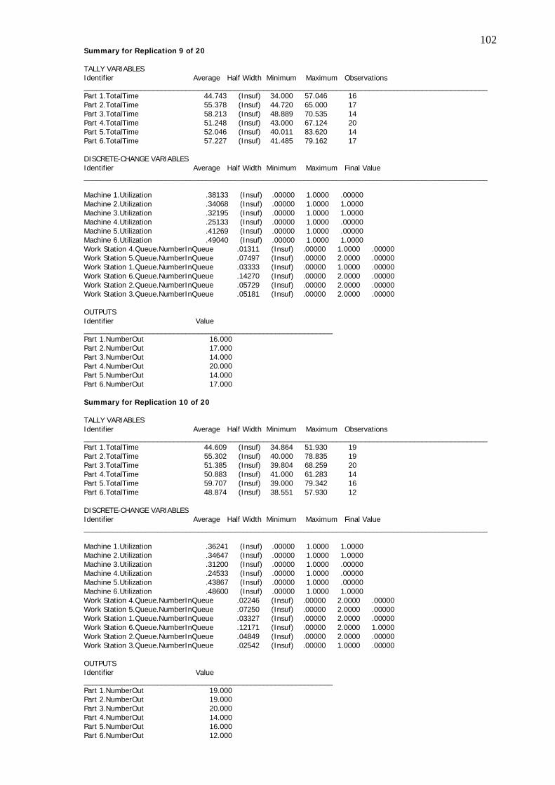
102Summary for Replication 9 of 20 TALLY VARIABLES Identifier Average Half Width Minimum Maximum Observations ___________________________________________________________________________________________________ Part 1.TotalTime 44.743 (Insuf) 34.000 57.046 16 Part 2.TotalTime 55.378 (Insuf) 44.720 65.000 17 Part 3.TotalTime 58.213 (Insuf) 48.889 70.535 14 Part 4.TotalTime 51.248 (Insuf) 43.000 67.124 20 Part 5.TotalTime 52.046 (Insuf) 40.011 83.620 14 Part 6.TotalTime 57.227 (Insuf) 41.485 79.162 17 DISCRETE-CHANGE VARIABLES Identifier Average Half Width Minimum Maximum Final Value ___________________________________________________________________________________________________ Machine 1.Utilization .38133 (Insuf) .00000 1.0000 .00000 Machine 2.Utilization .34068 (Insuf) .00000 1.0000 1.0000 Machine 3.Utilization .32195 (Insuf) .00000 1.0000 1.0000 Machine 4.Utilization .25133 (Insuf) .00000 1.0000 .00000 Machine 5.Utilization .41269 (Insuf) .00000 1.0000 .00000 Machine 6.Utilization .49040 (Insuf) .00000 1.0000 1.0000 Work Station 4.Queue.NumberInQueue .01311 (Insuf) .00000 1.0000 .00000 Work Station 5.Queue.NumberInQueue .07497 (Insuf) .00000 2.0000 .00000 Work Station 1.Queue.NumberInQueue .03333 (Insuf) .00000 1.0000 .00000 Work Station 6.Queue.NumberInQueue .14270 (Insuf) .00000 2.0000 .00000 Work Station 2.Queue.NumberInQueue .05729 (Insuf) .00000 2.0000 .00000 Work Station 3.Queue.NumberInQueue .05181 (Insuf) .00000 2.0000 .00000 OUTPUTS Identifier Value _____________________________________________________________ Part 1.NumberOut 16.000 Part 2.NumberOut 17.000 Part 3.NumberOut 14.000 Part 4.NumberOut 20.000 Part 5.NumberOut 14.000 Part 6.NumberOut 17.000 Summary for Replication 10 of 20 TALLY VARIABLES Identifier Average Half Width Minimum Maximum Observations ___________________________________________________________________________________________________ Part 1.TotalTime 44.609 (Insuf) 34.864 51.930 19 Part 2.TotalTime 55.302 (Insuf) 40.000 78.835 19 Part 3.TotalTime 51.385 (Insuf) 39.804 68.259 20 Part 4.TotalTime 50.883 (Insuf) 41.000 61.283 14 Part 5.TotalTime 59.707 (Insuf) 39.000 79.342 16 Part 6.TotalTime 48.874 (Insuf) 38.551 57.930 12 DISCRETE-CHANGE VARIABLES Identifier Average Half Width Minimum Maximum Final Value ___________________________________________________________________________________________________ Machine 1.Utilization .36241 (Insuf) .00000 1.0000 1.0000 Machine 2.Utilization .34647 (Insuf) .00000 1.0000 1.0000 Machine 3.Utilization .31200 (Insuf) .00000 1.0000 .00000 Machine 4.Utilization .24533 (Insuf) .00000 1.0000 .00000 Machine 5.Utilization .43867 (Insuf) .00000 1.0000 .00000 Machine 6.Utilization .48600 (Insuf) .00000 1.0000 1.0000 Work Station 4.Queue.NumberInQueue .02246 (Insuf) .00000 2.0000 .00000 Work Station 5.Queue.NumberInQueue .07250 (Insuf) .00000 2.0000 .00000 Work Station 1.Queue.NumberInQueue .03327 (Insuf) .00000 2.0000 .00000 Work Station 6.Queue.NumberInQueue .12171 (Insuf) .00000 2.0000 1.0000 Work Station 2.Queue.NumberInQueue .04849 (Insuf) .00000 2.0000 .00000 Work Station 3.Queue.NumberInQueue .02542 (Insuf) .00000 1.0000 .00000 OUTPUTS Identifier Value _____________________________________________________________ Part 1.NumberOut 19.000 Part 2.NumberOut 19.000 Part 3.NumberOut 20.000 Part 4.NumberOut 14.000 Part 5.NumberOut 16.000 Part 6.NumberOut 12.000

103Summary for Replication 11 of 20 TALLY VARIABLES Identifier Average Half Width Minimum Maximum Observations ___________________________________________________________________________________________________ Part 1.TotalTime 45.870 (Insuf) 40.000 52.495 16 Part 2.TotalTime 55.255 (Insuf) 41.869 65.972 17 Part 3.TotalTime 53.547 (Insuf) 38.000 75.815 18 Part 4.TotalTime 52.500 (Insuf) 37.000 66.410 21 Part 5.TotalTime 51.124 (Insuf) 42.808 57.106 13 Part 6.TotalTime 53.724 (Insuf) 37.201 72.349 17 DISCRETE-CHANGE VARIABLES Identifier Average Half Width Minimum Maximum Final Value ___________________________________________________________________________________________________ Machine 1.Utilization .35933 (Insuf) .00000 1.0000 .00000 Machine 2.Utilization .32660 (Insuf) .00000 1.0000 1.0000 Machine 3.Utilization .31281 (Insuf) .00000 1.0000 .00000 Machine 4.Utilization .25733 (Insuf) .00000 1.0000 .00000 Machine 5.Utilization .43614 (Insuf) .00000 1.0000 .00000 Machine 6.Utilization .46943 (Insuf) .00000 1.0000 1.0000 Work Station 4.Queue.NumberInQueue .02103 (Insuf) .00000 1.0000 .00000 Work Station 5.Queue.NumberInQueue .07837 (Insuf) .00000 2.0000 .00000 Work Station 1.Queue.NumberInQueue .04542 (Insuf) .00000 2.0000 .00000 Work Station 6.Queue.NumberInQueue .13448 (Insuf) .00000 2.0000 .00000 Work Station 2.Queue.NumberInQueue .03194 (Insuf) .00000 1.0000 .00000 Work Station 3.Queue.NumberInQueue .03726 (Insuf) .00000 1.0000 .00000 OUTPUTS Identifier Value _____________________________________________________________ Part 1.NumberOut 16.000 Part 2.NumberOut 17.000 Part 3.NumberOut 18.000 Part 4.NumberOut 21.000 Part 5.NumberOut 13.000 Part 6.NumberOut 17.000 Summary for Replication 12 of 20 TALLY VARIABLES Identifier Average Half Width Minimum Maximum Observations ___________________________________________________________________________________________________ Part 1.TotalTime 45.093 (Insuf) 34.000 54.176 11 Part 2.TotalTime 55.347 (Insuf) 44.000 66.726 19 Part 3.TotalTime 53.394 (Insuf) 41.819 69.420 19 Part 4.TotalTime 51.236 (Insuf) 43.000 63.858 14 Part 5.TotalTime 52.649 (Insuf) 39.000 64.106 21 Part 6.TotalTime 55.998 (Insuf) 46.729 63.776 18 DISCRETE-CHANGE VARIABLES Identifier Average Half Width Minimum Maximum Final Value ___________________________________________________________________________________________________ Machine 1.Utilization .41006 (Insuf) .00000 1.0000 1.0000 Machine 2.Utilization .33133 (Insuf) .00000 1.0000 .00000 Machine 3.Utilization .37200 (Insuf) .00000 1.0000 .00000 Machine 4.Utilization .23999 (Insuf) .00000 1.0000 1.0000 Machine 5.Utilization .45134 (Insuf) .00000 1.0000 1.0000 Machine 6.Utilization .48873 (Insuf) .00000 1.0000 1.0000 Work Station 4.Queue.NumberInQueue .01801 (Insuf) .00000 1.0000 .00000 Work Station 5.Queue.NumberInQueue .08041 (Insuf) .00000 2.0000 .00000 Work Station 1.Queue.NumberInQueue .02638 (Insuf) .00000 2.0000 .00000 Work Station 6.Queue.NumberInQueue .12074 (Insuf) .00000 2.0000 .00000 Work Station 2.Queue.NumberInQueue .03427 (Insuf) .00000 2.0000 .00000 Work Station 3.Queue.NumberInQueue .06846 (Insuf) .00000 2.0000 .00000 OUTPUTS Identifier Value _____________________________________________________________ Part 1.NumberOut 11.000 Part 2.NumberOut 19.000 Part 3.NumberOut 19.000 Part 4.NumberOut 14.000 Part 5.NumberOut 21.000 Part 6.NumberOut 18.000

104Summary for Replication 13 of 20 TALLY VARIABLES Identifier Average Half Width Minimum Maximum Observations ___________________________________________________________________________________________________ Part 1.TotalTime 45.816 (Insuf) 34.000 57.480 14 Part 2.TotalTime 56.326 (Insuf) 40.000 76.677 24 Part 3.TotalTime 54.848 (Insuf) 42.234 72.402 17 Part 4.TotalTime 52.772 (Insuf) 46.000 66.438 17 Part 5.TotalTime 53.018 (Insuf) 43.000 72.502 16 Part 6.TotalTime 56.647 (Insuf) 45.809 73.649 13 DISCRETE-CHANGE VARIABLES Identifier Average Half Width Minimum Maximum Final Value ___________________________________________________________________________________________________ Machine 1.Utilization .38480 (Insuf) .00000 1.0000 .00000 Machine 2.Utilization .34340 (Insuf) .00000 1.0000 1.0000 Machine 3.Utilization .32715 (Insuf) .00000 1.0000 1.0000 Machine 4.Utilization .26467 (Insuf) .00000 1.0000 .00000 Machine 5.Utilization .44133 (Insuf) .00000 1.0000 .00000 Machine 6.Utilization .49978 (Insuf) .00000 1.0000 1.0000 Work Station 4.Queue.NumberInQueue .02417 (Insuf) .00000 2.0000 .00000 Work Station 5.Queue.NumberInQueue .09296 (Insuf) .00000 2.0000 .00000 Work Station 1.Queue.NumberInQueue .03393 (Insuf) .00000 2.0000 .00000 Work Station 6.Queue.NumberInQueue .11763 (Insuf) .00000 2.0000 .00000 Work Station 2.Queue.NumberInQueue .02511 (Insuf) .00000 1.0000 .00000 Work Station 3.Queue.NumberInQueue .08304 (Insuf) .00000 3.0000 .00000 OUTPUTS Identifier Value _____________________________________________________________ Part 1.NumberOut 14.000 Part 2.NumberOut 24.000 Part 3.NumberOut 17.000 Part 4.NumberOut 17.000 Part 5.NumberOut 16.000 Part 6.NumberOut 13.000 Summary for Replication 14 of 20 TALLY VARIABLES Identifier Average Half Width Minimum Maximum Observations ___________________________________________________________________________________________________ Part 1.TotalTime 43.020 (Insuf) 35.214 50.325 10 Part 2.TotalTime 56.413 (Insuf) 40.000 71.468 19 Part 3.TotalTime 55.854 (Insuf) 43.021 78.827 22 Part 4.TotalTime 52.771 (Insuf) 43.000 66.191 17 Part 5.TotalTime 53.366 (Insuf) 39.000 66.988 21 Part 6.TotalTime 52.771 (Insuf) 38.159 63.565 13 DISCRETE-CHANGE VARIABLES Identifier Average Half Width Minimum Maximum Final Value ___________________________________________________________________________________________________ Machine 1.Utilization .37467 (Insuf) .00000 1.0000 .00000 Machine 2.Utilization .33000 (Insuf) .00000 1.0000 .00000 Machine 3.Utilization .37261 (Insuf) .00000 1.0000 1.0000 Machine 4.Utilization .23200 (Insuf) .00000 1.0000 .00000 Machine 5.Utilization .45184 (Insuf) .00000 1.0000 .00000 Machine 6.Utilization .51333 (Insuf) .00000 1.0000 .00000 Work Station 1.Queue.NumberInQueue .03259 (Insuf) .00000 2.0000 .00000 Work Station 2.Queue.NumberInQueue .03889 (Insuf) .00000 2.0000 .00000 Work Station 3.Queue.NumberInQueue .06971 (Insuf) .00000 2.0000 .00000 Work Station 4.Queue.NumberInQueue .02176 (Insuf) .00000 2.0000 .00000 Work Station 5.Queue.NumberInQueue .09070 (Insuf) .00000 2.0000 .00000 Work Station 6.Queue.NumberInQueue .12943 (Insuf) .00000 2.0000 .00000 OUTPUTS Identifier Value _____________________________________________________________ Part 1.NumberOut 10.000 Part 2.NumberOut 19.000 Part 3.NumberOut 22.000 Part 4.NumberOut 17.000 Part 5.NumberOut 21.000 Part 6.NumberOut 13.000

105Summary for Replication 15 of 20 TALLY VARIABLES Identifier Average Half Width Minimum Maximum Observations ___________________________________________________________________________________________________ Part 1.TotalTime 44.941 (Insuf) 36.000 51.215 12 Part 2.TotalTime 57.493 (Insuf) 42.000 74.713 27 Part 3.TotalTime 54.500 (Insuf) 44.059 62.346 9 Part 4.TotalTime 51.165 (Insuf) 39.000 64.912 18 Part 5.TotalTime 58.901 (Insuf) 42.000 75.720 15 Part 6.TotalTime 57.448 (Insuf) 41.367 70.292 19 DISCRETE-CHANGE VARIABLES Identifier Average Half Width Minimum Maximum Final Value ___________________________________________________________________________________________________ Machine 1.Utilization .39930 (Insuf) .00000 1.0000 .00000 Machine 2.Utilization .33772 (Insuf) .00000 1.0000 .00000 Machine 3.Utilization .31467 (Insuf) .00000 1.0000 .00000 Machine 4.Utilization .25733 (Insuf) .00000 1.0000 .00000 Machine 5.Utilization .46263 (Insuf) .00000 1.0000 .00000 Machine 6.Utilization .50702 (Insuf) .00000 1.0000 1.0000 Work Station 4.Queue.NumberInQueue .02292 (Insuf) .00000 1.0000 .00000 Work Station 5.Queue.NumberInQueue .11213 (Insuf) .00000 2.0000 .00000 Work Station 1.Queue.NumberInQueue .03578 (Insuf) .00000 2.0000 .00000 Work Station 6.Queue.NumberInQueue .15658 (Insuf) .00000 2.0000 .00000 Work Station 2.Queue.NumberInQueue .01613 (Insuf) .00000 1.0000 .00000 Work Station 3.Queue.NumberInQueue .06775 (Insuf) .00000 2.0000 .00000 OUTPUTS Identifier Value _____________________________________________________________ Part 1.NumberOut 12.000 Part 2.NumberOut 27.000 Part 3.NumberOut 9.0000 Part 4.NumberOut 18.000 Part 5.NumberOut 15.000 Part 6.NumberOut 19.000 Summary for Replication 16 of 20 TALLY VARIABLES Identifier Average Half Width Minimum Maximum Observations ___________________________________________________________________________________________________ Part 1.TotalTime 41.992 (Insuf) 34.000 52.852 16 Part 2.TotalTime 55.347 (Insuf) 44.557 78.018 14 Part 3.TotalTime 51.950 (Insuf) 41.181 76.276 15 Part 4.TotalTime 52.089 (Insuf) 45.861 66.479 16 Part 5.TotalTime 53.664 (Insuf) 44.000 75.000 19 Part 6.TotalTime 53.779 (Insuf) 40.313 67.051 20 DISCRETE-CHANGE VARIABLES Identifier Average Half Width Minimum Maximum Final Value ___________________________________________________________________________________________________ Machine 1.Utilization .36038 (Insuf) .00000 1.0000 1.0000 Machine 2.Utilization .31867 (Insuf) .00000 1.0000 .00000 Machine 3.Utilization .32117 (Insuf) .00000 1.0000 1.0000 Machine 4.Utilization .23800 (Insuf) .00000 1.0000 .00000 Machine 5.Utilization .42657 (Insuf) .00000 1.0000 1.0000 Machine 6.Utilization .47133 (Insuf) .00000 1.0000 .00000 Work Station 4.Queue.NumberInQueue .01166 (Insuf) .00000 1.0000 .00000 Work Station 5.Queue.NumberInQueue .06206 (Insuf) .00000 1.0000 .00000 Work Station 1.Queue.NumberInQueue .04238 (Insuf) .00000 2.0000 .00000 Work Station 6.Queue.NumberInQueue .15366 (Insuf) .00000 2.0000 .00000 Work Station 2.Queue.NumberInQueue .04427 (Insuf) .00000 2.0000 .00000 Work Station 3.Queue.NumberInQueue .06129 (Insuf) .00000 2.0000 .00000 OUTPUTS Identifier Value _____________________________________________________________ Part 1.NumberOut 16.000 Part 2.NumberOut 14.000 Part 3.NumberOut 15.000 Part 4.NumberOut 16.000 Part 5.NumberOut 19.000 Part 6.NumberOut 20.000

106Summary for Replication 17 of 20 TALLY VARIABLES Identifier Average Half Width Minimum Maximum Observations ___________________________________________________________________________________________________ Part 1.TotalTime 47.011 (Insuf) 34.234 63.573 9 Part 2.TotalTime 53.503 (Insuf) 39.562 65.965 14 Part 3.TotalTime 50.816 (Insuf) 39.000 71.377 18 Part 4.TotalTime 51.273 (Insuf) 39.296 61.607 22 Part 5.TotalTime 54.766 (Insuf) 43.126 64.214 21 Part 6.TotalTime 53.550 (Insuf) 42.561 68.697 17 DISCRETE-CHANGE VARIABLES Identifier Average Half Width Minimum Maximum Final Value ___________________________________________________________________________________________________ Machine 1.Utilization .39917 (Insuf) .00000 1.0000 1.0000 Machine 2.Utilization .31915 (Insuf) .00000 1.0000 .00000 Machine 3.Utilization .35318 (Insuf) .00000 1.0000 1.0000 Machine 4.Utilization .22867 (Insuf) .00000 1.0000 .00000 Machine 5.Utilization .43954 (Insuf) .00000 1.0000 1.0000 Machine 6.Utilization .50724 (Insuf) .00000 1.0000 1.0000 Work Station 4.Queue.NumberInQueue .01429 (Insuf) .00000 1.0000 .00000 Work Station 5.Queue.NumberInQueue .07393 (Insuf) .00000 2.0000 .00000 Work Station 1.Queue.NumberInQueue .02814 (Insuf) .00000 2.0000 .00000 Work Station 6.Queue.NumberInQueue .11765 (Insuf) .00000 2.0000 .00000 Work Station 2.Queue.NumberInQueue .04381 (Insuf) .00000 2.0000 .00000 Work Station 3.Queue.NumberInQueue .08176 (Insuf) .00000 3.0000 .00000 OUTPUTS Identifier Value _____________________________________________________________ Part 1.NumberOut 9.0000 Part 2.NumberIn 15.000 Part 2.NumberOut 14.000 Part 3.NumberOut 18.000 Part 4.NumberOut 22.000 Part 5.NumberOut 21.000 Part 6.NumberOut 17.000 Summary for Replication 18 of 20 TALLY VARIABLES Identifier Average Half Width Minimum Maximum Observations ___________________________________________________________________________________________________ Part 1.TotalTime 46.351 (Insuf) 34.000 55.769 15 Part 2.TotalTime 55.154 (Insuf) 44.000 72.506 17 Part 3.TotalTime 51.494 (Insuf) 41.000 64.768 20 Part 4.TotalTime 51.949 (Insuf) 40.292 65.791 18 Part 5.TotalTime 58.042 (Insuf) 39.000 88.603 13 Part 6.TotalTime 52.399 (Insuf) 37.970 67.863 19 DISCRETE-CHANGE VARIABLES Identifier Average Half Width Minimum Maximum Final Value ___________________________________________________________________________________________________ Machine 1.Utilization .38267 (Insuf) .00000 1.0000 .00000 Machine 2.Utilization .32781 (Insuf) .00000 1.0000 1.0000 Machine 3.Utilization .31445 (Insuf) .00000 1.0000 .00000 Machine 4.Utilization .24723 (Insuf) .00000 1.0000 1.0000 Machine 5.Utilization .42778 (Insuf) .00000 1.0000 .00000 Machine 6.Utilization .50333 (Insuf) .00000 1.0000 .00000 Work Station 4.Queue.NumberInQueue .03439 (Insuf) .00000 2.0000 1.0000 Work Station 5.Queue.NumberInQueue .05171 (Insuf) .00000 2.0000 .00000 Work Station 1.Queue.NumberInQueue .03522 (Insuf) .00000 2.0000 .00000 Work Station 6.Queue.NumberInQueue .15524 (Insuf) .00000 3.0000 .00000 Work Station 2.Queue.NumberInQueue .03218 (Insuf) .00000 2.0000 .00000 Work Station 3.Queue.NumberInQueue .07265 (Insuf) .00000 2.0000 .00000 OUTPUTS Identifier Value _____________________________________________________________ Part 1.NumberOut 15.000 Part 2.NumberOut 17.000 Part 3.NumberOut 20.000 Part 4.NumberOut 18.000 Part 5.NumberOut 13.000 Part 6.NumberOut 19.000

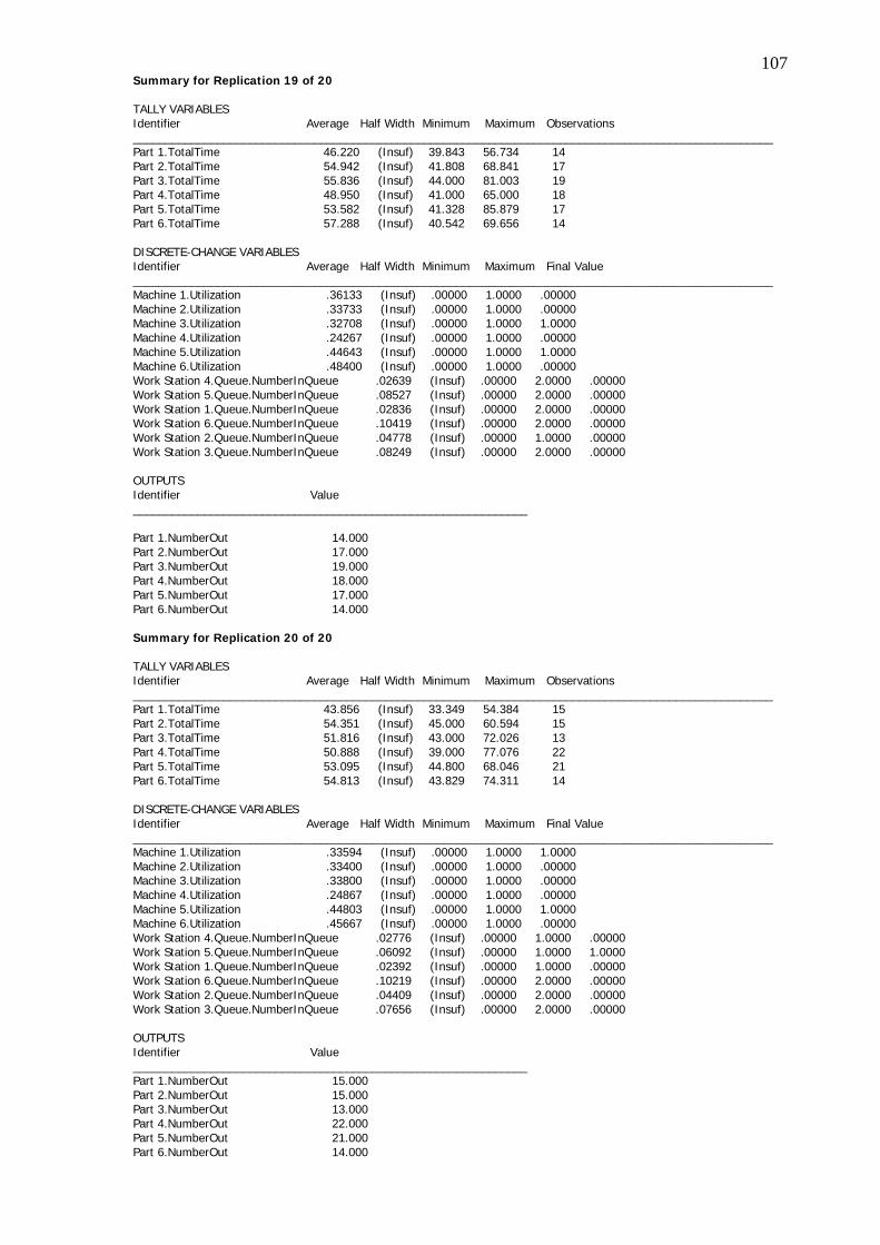
107Summary for Replication 19 of 20 TALLY VARIABLES Identifier Average Half Width Minimum Maximum Observations ___________________________________________________________________________________________________ Part 1.TotalTime 46.220 (Insuf) 39.843 56.734 14 Part 2.TotalTime 54.942 (Insuf) 41.808 68.841 17 Part 3.TotalTime 55.836 (Insuf) 44.000 81.003 19 Part 4.TotalTime 48.950 (Insuf) 41.000 65.000 18 Part 5.TotalTime 53.582 (Insuf) 41.328 85.879 17 Part 6.TotalTime 57.288 (Insuf) 40.542 69.656 14 DISCRETE-CHANGE VARIABLES Identifier Average Half Width Minimum Maximum Final Value ___________________________________________________________________________________________________ Machine 1.Utilization .36133 (Insuf) .00000 1.0000 .00000 Machine 2.Utilization .33733 (Insuf) .00000 1.0000 .00000 Machine 3.Utilization .32708 (Insuf) .00000 1.0000 1.0000 Machine 4.Utilization .24267 (Insuf) .00000 1.0000 .00000 Machine 5.Utilization .44643 (Insuf) .00000 1.0000 1.0000 Machine 6.Utilization .48400 (Insuf) .00000 1.0000 .00000 Work Station 4.Queue.NumberInQueue .02639 (Insuf) .00000 2.0000 .00000 Work Station 5.Queue.NumberInQueue .08527 (Insuf) .00000 2.0000 .00000 Work Station 1.Queue.NumberInQueue .02836 (Insuf) .00000 2.0000 .00000 Work Station 6.Queue.NumberInQueue .10419 (Insuf) .00000 2.0000 .00000 Work Station 2.Queue.NumberInQueue .04778 (Insuf) .00000 1.0000 .00000 Work Station 3.Queue.NumberInQueue .08249 (Insuf) .00000 2.0000 .00000 OUTPUTS Identifier Value _____________________________________________________________ Part 1.NumberOut 14.000 Part 2.NumberOut 17.000 Part 3.NumberOut 19.000 Part 4.NumberOut 18.000 Part 5.NumberOut 17.000 Part 6.NumberOut 14.000 Summary for Replication 20 of 20 TALLY VARIABLES Identifier Average Half Width Minimum Maximum Observations ___________________________________________________________________________________________________ Part 1.TotalTime 43.856 (Insuf) 33.349 54.384 15 Part 2.TotalTime 54.351 (Insuf) 45.000 60.594 15 Part 3.TotalTime 51.816 (Insuf) 43.000 72.026 13 Part 4.TotalTime 50.888 (Insuf) 39.000 77.076 22 Part 5.TotalTime 53.095 (Insuf) 44.800 68.046 21 Part 6.TotalTime 54.813 (Insuf) 43.829 74.311 14 DISCRETE-CHANGE VARIABLES Identifier Average Half Width Minimum Maximum Final Value ___________________________________________________________________________________________________ Machine 1.Utilization .33594 (Insuf) .00000 1.0000 1.0000 Machine 2.Utilization .33400 (Insuf) .00000 1.0000 .00000 Machine 3.Utilization .33800 (Insuf) .00000 1.0000 .00000 Machine 4.Utilization .24867 (Insuf) .00000 1.0000 .00000 Machine 5.Utilization .44803 (Insuf) .00000 1.0000 1.0000 Machine 6.Utilization .45667 (Insuf) .00000 1.0000 .00000 Work Station 4.Queue.NumberInQueue .02776 (Insuf) .00000 1.0000 .00000 Work Station 5.Queue.NumberInQueue .06092 (Insuf) .00000 1.0000 1.0000 Work Station 1.Queue.NumberInQueue .02392 (Insuf) .00000 1.0000 .00000 Work Station 6.Queue.NumberInQueue .10219 (Insuf) .00000 2.0000 .00000 Work Station 2.Queue.NumberInQueue .04409 (Insuf) .00000 2.0000 .00000 Work Station 3.Queue.NumberInQueue .07656 (Insuf) .00000 2.0000 .00000 OUTPUTS Identifier Value _____________________________________________________________ Part 1.NumberOut 15.000 Part 2.NumberOut 15.000 Part 3.NumberOut 13.000 Part 4.NumberOut 22.000 Part 5.NumberOut 21.000 Part 6.NumberOut 14.000

108 Summary for Replication 1 of 20 TALLY VARIABLES Identifier Average Half Width Minimum Maximum Observations ___________________________________________________________________________________________________ Part 1.TotalTime 48.081 (Insuf) 32.636 64.711 21 Part 2.TotalTime 61.781 (Insuf) 49.000 81.247 24 Part 3.TotalTime 56.961 (Insuf) 41.538 80.614 23 Part 4.TotalTime 56.643 (Insuf) 37.558 84.507 30 Part 5.TotalTime 61.968 (Insuf) 47.000 80.000 26 Part 6.TotalTime 54.669 (Insuf) 44.309 83.650 27 DISCRETE-CHANGE VARIABLES Identifier Average Half Width Minimum Maximum Final Value ___________________________________________________________________________________________________ Machine 1.Utilization .57577 (Insuf) .00000 1.0000 .00000 Machine 2.Utilization .47333 (Insuf) .00000 1.0000 .00000 Machine 3.Utilization .43444 (Insuf) .00000 1.0000 .00000 Machine 4.Utilization .37068 (Insuf) .00000 1.0000 1.0000 Machine 5.Utilization .64377 (Insuf) .00000 1.0000 1.0000 Machine 6.Utilization .67310 (Insuf) .00000 1.0000 .00000 Work Station 4.Queue.NumberInQueue .08105 (Insuf) .00000 3.0000 .00000 Work Station 5.Queue.NumberInQueue .21839 (Insuf) .00000 3.0000 1.0000 Work Station 1.Queue.NumberInQueue .09901 (Insuf) .00000 2.0000 .00000 Work Station 6.Queue.NumberInQueue .44552 (Insuf) .00000 4.0000 .00000 Work Station 2.Queue.NumberInQueue .13939 (Insuf) .00000 3.0000 .00000 Work Station 3.Queue.NumberInQueue .11514 (Insuf) .00000 3.0000 .00000 OUTPUTS Identifier Value _____________________________________________________________ Part 1.NumberOut 21.000 Part 2.NumberOut 24.000 Part 3.NumberOut 23.000 Part 4.NumberOut 30.000 Part 5.NumberOut 26.000 Part 6.NumberOut 27.000 Summary for Replication 2 of 20 TALLY VARIABLES Identifier Average Half Width Minimum Maximum Observations ___________________________________________________________________________________________________ Part 1.TotalTime 47.015 (Insuf) 33.000 58.313 19 Part 2.TotalTime 60.420 (Insuf) 43.000 86.195 25 Part 3.TotalTime 57.586 (Insuf) 41.869 79.787 32 Part 4.TotalTime 59.309 (Insuf) 43.444 75.420 20 Part 5.TotalTime 58.200 (Insuf) 42.000 83.603 30 Part 6.TotalTime 60.720 (Insuf) 36.034 82.638 22 DISCRETE-CHANGE VARIABLES Identifier Average Half Width Minimum Maximum Final Value ___________________________________________________________________________________________________ Machine 1.Utilization .55102 (Insuf) .00000 1.0000 1.0000 Machine 2.Utilization .46133 (Insuf) .00000 1.0000 .00000 Machine 3.Utilization .48133 (Insuf) .00000 1.0000 .00000 Machine 4.Utilization .34215 (Insuf) .00000 1.0000 1.0000 Machine 5.Utilization .65536 (Insuf) .00000 1.0000 .00000 Machine 6.Utilization .67368 (Insuf) .00000 1.0000 1.0000 Work Station 4.Queue.NumberInQueue .06004 (Insuf) .00000 2.0000 .00000 Work Station 5.Queue.NumberInQueue .31365 (Insuf) .00000 4.0000 .00000 Work Station 1.Queue.NumberInQueue .12775 (Insuf) .00000 2.0000 .00000 Work Station 6.Queue.NumberInQueue .38306 (Insuf) .00000 3.0000 1.0000 Work Station 2.Queue.NumberInQueue .13461 (Insuf) .00000 2.0000 .00000 Work Station 3.Queue.NumberInQueue .18582 (Insuf) .00000 3.0000 .00000 OUTPUTS Identifier Value _____________________________________________________________ Part 1.NumberOut 19.000 Part 2.NumberOut 25.000 Part 3.NumberOut 32.000 Part 4.NumberOut 20.000 Part 5.NumberOut 30.000 Part 6.NumberOut 22.000

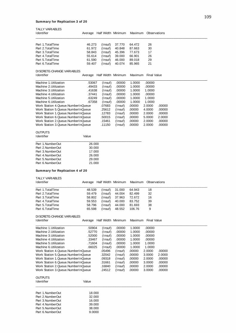
109Summary for Replication 3 of 20 TALLY VARIABLES Identifier Average Half Width Minimum Maximum Observations ___________________________________________________________________________________________________ Part 1.TotalTime 46.273 (Insuf) 37.770 64.472 26 Part 2.TotalTime 61.972 (Insuf) 40.848 87.663 30 Part 3.TotalTime 58.843 (Insuf) 45.396 77.673 17 Part 4.TotalTime 55.614 (Insuf) 39.000 66.901 26 Part 5.TotalTime 61.590 (Insuf) 46.000 89.018 29 Part 6.TotalTime 59.407 (Insuf) 40.074 85.965 21 DISCRETE-CHANGE VARIABLES Identifier Average Half Width Minimum Maximum Final Value ___________________________________________________________________________________________________ Machine 1.Utilization .53067 (Insuf) .00000 1.0000 .00000 Machine 2.Utilization .49433 (Insuf) .00000 1.0000 .00000 Machine 3.Utilization .41638 (Insuf) .00000 1.0000 1.0000 Machine 4.Utilization .37441 (Insuf) .00000 1.0000 .00000 Machine 5.Utilization .63249 (Insuf) .00000 1.0000 1.0000 Machine 6.Utilization .67358 (Insuf) .00000 1.0000 1.0000 Work Station 4.Queue.NumberInQueue .07683 (Insuf) .00000 2.0000 .00000 Work Station 5.Queue.NumberInQueue .25612 (Insuf) .00000 4.0000 .00000 Work Station 1.Queue.NumberInQueue .12783 (Insuf) .00000 2.0000 .00000 Work Station 6.Queue.NumberInQueue .50015 (Insuf) .00000 5.0000 2.0000 Work Station 2.Queue.NumberInQueue .15461 (Insuf) .00000 2.0000 .00000 Work Station 3.Queue.NumberInQueue .11150 (Insuf) .00000 2.0000 .00000 OUTPUTS Identifier Value _____________________________________________________________ Part 1.NumberOut 26.000 Part 2.NumberOut 30.000 Part 3.NumberOut 17.000 Part 4.NumberOut 26.000 Part 5.NumberOut 29.000 Part 6.NumberOut 21.000 Summary for Replication 4 of 20 TALLY VARIABLES Identifier Average Half Width Minimum Maximum Observations ___________________________________________________________________________________________________ Part 1.TotalTime 48.539 (Insuf) 31.000 64.943 18 Part 2.TotalTime 59.479 (Insuf) 44.004 82.499 32 Part 3.TotalTime 58.802 (Insuf) 37.963 72.672 16 Part 4.TotalTime 59.553 (Insuf) 40.000 83.752 39 Part 5.TotalTime 58.796 (Insuf) 44.000 81.693 38 Part 6.TotalTime 65.598 (Insuf) 48.552 106.76 9 DISCRETE-CHANGE VARIABLES Identifier Average Half Width Minimum Maximum Final Value ___________________________________________________________________________________________________ Machine 1.Utilization .50904 (Insuf) .00000 1.0000 .00000 Machine 2.Utilization .52770 (Insuf) .00000 1.0000 .00000 Machine 3.Utilization .52000 (Insuf) .00000 1.0000 .00000 Machine 4.Utilization .33467 (Insuf) .00000 1.0000 .00000 Machine 5.Utilization .71604 (Insuf) .00000 1.0000 1.0000 Machine 6.Utilization .66025 (Insuf) .00000 1.0000 1.0000 Work Station 4.Queue.NumberInQueue .05496 (Insuf) .00000 2.0000 .00000 Work Station 5.Queue.NumberInQueue .32042 (Insuf) .00000 3.0000 2.0000 Work Station 1.Queue.NumberInQueue .09318 (Insuf) .00000 2.0000 .00000 Work Station 6.Queue.NumberInQueue .31661 (Insuf) .00000 3.0000 .00000 Work Station 2.Queue.NumberInQueue .16840 (Insuf) .00000 2.0000 .00000 Work Station 3.Queue.NumberInQueue .24512 (Insuf) .00000 3.0000 .00000 OUTPUTS Identifier Value _____________________________________________________________ Part 1.NumberOut 18.000 Part 2.NumberOut 32.000 Part 3.NumberOut 16.000 Part 4.NumberOut 39.000 Part 5.NumberOut 38.000 Part 6.NumberOut 9.0000

110Summary for Replication 5 of 20 TALLY VARIABLES Identifier Average Half Width Minimum Maximum Observations ___________________________________________________________________________________________________ Part 1.TotalTime 48.876 (Insuf) 33.967 73.941 23 Part 2.TotalTime 63.090 (Insuf) 36.000 92.000 27 Part 3.TotalTime 61.680 (Insuf) 41.165 87.191 26 Part 4.TotalTime 64.135 (Insuf) 40.000 95.028 29 Part 5.TotalTime 61.552 (Insuf) 47.458 81.227 26 Part 6.TotalTime 65.625 (Insuf) 41.030 86.342 18 DISCRETE-CHANGE VARIABLES Identifier Average Half Width Minimum Maximum Final Value ___________________________________________________________________________________________________ Machine 1.Utilization .59839 (Insuf) .00000 1.0000 1.0000 Machine 2.Utilization .49760 (Insuf) .00000 1.0000 1.0000 Machine 3.Utilization .47215 (Insuf) .00000 1.0000 1.0000 Machine 4.Utilization .37784 (Insuf) .00000 1.0000 1.0000 Machine 5.Utilization .68552 (Insuf) .00000 1.0000 1.0000 Machine 6.Utilization .67572 (Insuf) .00000 1.0000 1.0000 Work Station 4.Queue.NumberInQueue .07811 (Insuf) .00000 2.0000 .00000 Work Station 5.Queue.NumberInQueue .39687 (Insuf) .00000 4.0000 1.0000 Work Station 1.Queue.NumberInQueue .15077 (Insuf) .00000 2.0000 .00000 Work Station 6.Queue.NumberInQueue .46077 (Insuf) .00000 5.0000 .00000 Work Station 2.Queue.NumberInQueue .21522 (Insuf) .00000 2.0000 1.0000 Work Station 3.Queue.NumberInQueue .20203 (Insuf) .00000 3.0000 .00000 OUTPUTS Identifier Value _____________________________________________________________ Part 1.NumberOut 23.000 Part 2.NumberOut 27.000 Part 3.NumberOut 26.000 Part 4.NumberOut 29.000 Part 5.NumberOut 26.000 Part 6.NumberOut 18.000 Summary for Replication 6 of 20 TALLY VARIABLES Identifier Average Half Width Minimum Maximum Observations ___________________________________________________________________________________________________ Part 1.TotalTime 49.244 (Insuf) 36.198 63.332 28 Part 2.TotalTime 61.740 (Insuf) 43.003 75.773 31 Part 3.TotalTime 66.280 (Insuf) 49.119 94.495 16 Part 4.TotalTime 56.122 (Insuf) 40.000 77.569 31 Part 5.TotalTime 58.001 (Insuf) 42.728 89.376 29 Part 6.TotalTime 63.918 (Insuf) 37.152 94.542 20 DISCRETE-CHANGE VARIABLES Identifier Average Half Width Minimum Maximum Final Value ___________________________________________________________________________________________________ Machine 1.Utilization .55643 (Insuf) .00000 1.0000 1.0000 Machine 2.Utilization .52156 (Insuf) .00000 1.0000 1.0000 Machine 3.Utilization .44733 (Insuf) .00000 1.0000 .00000 Machine 4.Utilization .38748 (Insuf) .00000 1.0000 1.0000 Machine 5.Utilization .68067 (Insuf) .00000 1.0000 .00000 Machine 6.Utilization .66602 (Insuf) .00000 1.0000 1.0000 Work Station 1.Queue.NumberInQueue .13514 (Insuf) .00000 2.0000 .00000 Work Station 2.Queue.NumberInQueue .17216 (Insuf) .00000 3.0000 1.0000 Work Station 3.Queue.NumberInQueue .18505 (Insuf) .00000 3.0000 .00000 Work Station 4.Queue.NumberInQueue .08265 (Insuf) .00000 2.0000 .00000 Work Station 5.Queue.NumberInQueue .34975 (Insuf) .00000 3.0000 .00000 Work Station 6.Queue.NumberInQueue .42096 (Insuf) .00000 3.0000 .00000 OUTPUTS Identifier Value _____________________________________________________________ Part 1.NumberOut 28.000 Part 2.NumberOut 31.000 Part 3.NumberOut 16.000 Part 4.NumberOut 31.000 Part 5.NumberOut 29.000 Part 6.NumberOut 20.000

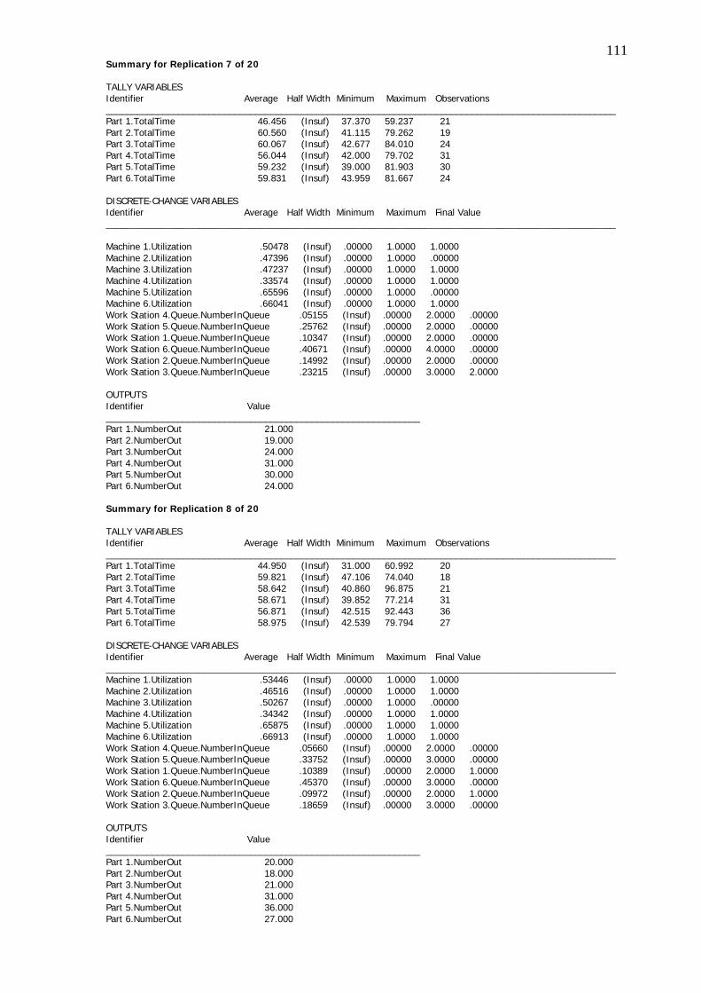
111Summary for Replication 7 of 20 TALLY VARIABLES Identifier Average Half Width Minimum Maximum Observations ___________________________________________________________________________________________________ Part 1.TotalTime 46.456 (Insuf) 37.370 59.237 21 Part 2.TotalTime 60.560 (Insuf) 41.115 79.262 19 Part 3.TotalTime 60.067 (Insuf) 42.677 84.010 24 Part 4.TotalTime 56.044 (Insuf) 42.000 79.702 31 Part 5.TotalTime 59.232 (Insuf) 39.000 81.903 30 Part 6.TotalTime 59.831 (Insuf) 43.959 81.667 24 DISCRETE-CHANGE VARIABLES Identifier Average Half Width Minimum Maximum Final Value ___________________________________________________________________________________________________ Machine 1.Utilization .50478 (Insuf) .00000 1.0000 1.0000 Machine 2.Utilization .47396 (Insuf) .00000 1.0000 .00000 Machine 3.Utilization .47237 (Insuf) .00000 1.0000 1.0000 Machine 4.Utilization .33574 (Insuf) .00000 1.0000 1.0000 Machine 5.Utilization .65596 (Insuf) .00000 1.0000 .00000 Machine 6.Utilization .66041 (Insuf) .00000 1.0000 1.0000 Work Station 4.Queue.NumberInQueue .05155 (Insuf) .00000 2.0000 .00000 Work Station 5.Queue.NumberInQueue .25762 (Insuf) .00000 2.0000 .00000 Work Station 1.Queue.NumberInQueue .10347 (Insuf) .00000 2.0000 .00000 Work Station 6.Queue.NumberInQueue .40671 (Insuf) .00000 4.0000 .00000 Work Station 2.Queue.NumberInQueue .14992 (Insuf) .00000 2.0000 .00000 Work Station 3.Queue.NumberInQueue .23215 (Insuf) .00000 3.0000 2.0000 OUTPUTS Identifier Value _____________________________________________________________ Part 1.NumberOut 21.000 Part 2.NumberOut 19.000 Part 3.NumberOut 24.000 Part 4.NumberOut 31.000 Part 5.NumberOut 30.000 Part 6.NumberOut 24.000 Summary for Replication 8 of 20 TALLY VARIABLES Identifier Average Half Width Minimum Maximum Observations ___________________________________________________________________________________________________ Part 1.TotalTime 44.950 (Insuf) 31.000 60.992 20 Part 2.TotalTime 59.821 (Insuf) 47.106 74.040 18 Part 3.TotalTime 58.642 (Insuf) 40.860 96.875 21 Part 4.TotalTime 58.671 (Insuf) 39.852 77.214 31 Part 5.TotalTime 56.871 (Insuf) 42.515 92.443 36 Part 6.TotalTime 58.975 (Insuf) 42.539 79.794 27 DISCRETE-CHANGE VARIABLES Identifier Average Half Width Minimum Maximum Final Value ___________________________________________________________________________________________________ Machine 1.Utilization .53446 (Insuf) .00000 1.0000 1.0000 Machine 2.Utilization .46516 (Insuf) .00000 1.0000 1.0000 Machine 3.Utilization .50267 (Insuf) .00000 1.0000 .00000 Machine 4.Utilization .34342 (Insuf) .00000 1.0000 1.0000 Machine 5.Utilization .65875 (Insuf) .00000 1.0000 1.0000 Machine 6.Utilization .66913 (Insuf) .00000 1.0000 1.0000 Work Station 4.Queue.NumberInQueue .05660 (Insuf) .00000 2.0000 .00000 Work Station 5.Queue.NumberInQueue .33752 (Insuf) .00000 3.0000 .00000 Work Station 1.Queue.NumberInQueue .10389 (Insuf) .00000 2.0000 1.0000 Work Station 6.Queue.NumberInQueue .45370 (Insuf) .00000 3.0000 .00000 Work Station 2.Queue.NumberInQueue .09972 (Insuf) .00000 2.0000 1.0000 Work Station 3.Queue.NumberInQueue .18659 (Insuf) .00000 3.0000 .00000 OUTPUTS Identifier Value _____________________________________________________________ Part 1.NumberOut 20.000 Part 2.NumberOut 18.000 Part 3.NumberOut 21.000 Part 4.NumberOut 31.000 Part 5.NumberOut 36.000 Part 6.NumberOut 27.000

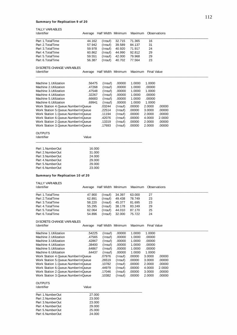
112Summary for Replication 9 of 20 TALLY VARIABLES Identifier Average Half Width Minimum Maximum Observations ___________________________________________________________________________________________________ Part 1.TotalTime 44.162 (Insuf) 32.715 71.365 16 Part 2.TotalTime 57.942 (Insuf) 39.589 84.137 31 Part 3.TotalTime 59.978 (Insuf) 40.920 71.917 24 Part 4.TotalTime 60.862 (Insuf) 44.990 92.812 29 Part 5.TotalTime 59.551 (Insuf) 42.000 79.968 29 Part 6.TotalTime 56.387 (Insuf) 40.702 77.564 23 DISCRETE-CHANGE VARIABLES Identifier Average Half Width Minimum Maximum Final Value ___________________________________________________________________________________________________ Machine 1.Utilization .56475 (Insuf) .00000 1.0000 1.0000 Machine 2.Utilization .47268 (Insuf) .00000 1.0000 .00000 Machine 3.Utilization .47548 (Insuf) .00000 1.0000 1.0000 Machine 4.Utilization .32267 (Insuf) .00000 1.0000 .00000 Machine 5.Utilization .66683 (Insuf) .00000 1.0000 .00000 Machine 6.Utilization .69941 (Insuf) .00000 1.0000 1.0000 Work Station 4.Queue.NumberInQueue .03244 (Insuf) .00000 2.0000 .00000 Work Station 5.Queue.NumberInQueue .22514 (Insuf) .00000 3.0000 .00000 Work Station 1.Queue.NumberInQueue .11194 (Insuf) .00000 2.0000 .00000 Work Station 6.Queue.NumberInQueue .42076 (Insuf) .00000 4.0000 2.0000 Work Station 2.Queue.NumberInQueue .13319 (Insuf) .00000 2.0000 .00000 Work Station 3.Queue.NumberInQueue .17693 (Insuf) .00000 2.0000 .00000 OUTPUTS Identifier Value _____________________________________________________________ Part 1.NumberOut 16.000 Part 2.NumberOut 31.000 Part 3.NumberOut 24.000 Part 4.NumberOut 29.000 Part 5.NumberOut 29.000 Part 6.NumberOut 23.000 Summary for Replication 10 of 20 TALLY VARIABLES Identifier Average Half Width Minimum Maximum Observations ___________________________________________________________________________________________________ Part 1.TotalTime 47.900 (Insuf) 34.397 63.000 27 Part 2.TotalTime 62.891 (Insuf) 49.438 78.749 23 Part 3.TotalTime 58.220 (Insuf) 45.377 81.695 23 Part 4.TotalTime 55.295 (Insuf) 38.178 83.249 29 Part 5.TotalTime 62.064 (Insuf) 44.010 87.170 25 Part 6.TotalTime 54.896 (Insuf) 32.000 75.722 24 DISCRETE-CHANGE VARIABLES Identifier Average Half Width Minimum Maximum Final Value ___________________________________________________________________________________________________ Machine 1.Utilization .54225 (Insuf) .00000 1.0000 1.0000 Machine 2.Utilization .47565 (Insuf) .00000 1.0000 .00000 Machine 3.Utilization .42867 (Insuf) .00000 1.0000 .00000 Machine 4.Utilization .38400 (Insuf) .00000 1.0000 .00000 Machine 5.Utilization .64867 (Insuf) .00000 1.0000 .00000 Machine 6.Utilization .64437 (Insuf) .00000 1.0000 1.0000 Work Station 4.Queue.NumberInQueue .07976 (Insuf) .00000 3.0000 .00000 Work Station 5.Queue.NumberInQueue .26519 (Insuf) .00000 3.0000 .00000 Work Station 1.Queue.NumberInQueue .10782 (Insuf) .00000 2.0000 .00000 Work Station 6.Queue.NumberInQueue .44979 (Insuf) .00000 4.0000 2.0000 Work Station 2.Queue.NumberInQueue .17046 (Insuf) .00000 3.0000 .00000 Work Station 3.Queue.NumberInQueue .10382 (Insuf) .00000 2.0000 .00000 OUTPUTS Identifier Value _____________________________________________________________ Part 1.NumberOut 27.000 Part 2.NumberOut 23.000 Part 3.NumberOut 23.000 Part 4.NumberOut 29.000 Part 5.NumberOut 25.000 Part 6.NumberOut 24.000

113Summary for Replication 11 of 20 TALLY VARIABLES Identifier Average Half Width Minimum Maximum Observations ___________________________________________________________________________________________________ Part 1.TotalTime 49.834 (Insuf) 39.169 62.737 22 Part 2.TotalTime 62.484 (Insuf) 43.121 90.230 26 Part 3.TotalTime 55.907 (Insuf) 43.157 73.934 25 Part 4.TotalTime 57.895 (Insuf) 41.412 78.354 28 Part 5.TotalTime 60.134 (Insuf) 44.972 75.836 19 Part 6.TotalTime 58.279 (Insuf) 43.309 78.332 28 DISCRETE-CHANGE VARIABLES Identifier Average Half Width Minimum Maximum Final Value ___________________________________________________________________________________________________ Machine 1.Utilization .57190 (Insuf) .00000 1.0000 1.0000 Machine 2.Utilization .46887 (Insuf) .00000 1.0000 1.0000 Machine 3.Utilization .40005 (Insuf) .00000 1.0000 1.0000 Machine 4.Utilization .37267 (Insuf) .00000 1.0000 .00000 Machine 5.Utilization .66370 (Insuf) .00000 1.0000 1.0000 Machine 6.Utilization .71014 (Insuf) .00000 1.0000 .00000 Work Station 4.Queue.NumberInQueue .08785 (Insuf) .00000 2.0000 .00000 Work Station 5.Queue.NumberInQueue .23852 (Insuf) .00000 3.0000 .00000 Work Station 1.Queue.NumberInQueue .08398 (Insuf) .00000 2.0000 1.0000 Work Station 6.Queue.NumberInQueue .49973 (Insuf) .00000 4.0000 .00000 Work Station 2.Queue.NumberInQueue .09449 (Insuf) .00000 2.0000 .00000 Work Station 3.Queue.NumberInQueue .10657 (Insuf) .00000 2.0000 .00000 OUTPUTS Identifier Value _____________________________________________________________ Part 1.NumberOut 22.000 Part 2.NumberOut 26.000 Part 3.NumberOut 25.000 Part 4.NumberOut 28.000 Part 5.NumberOut 19.000 Part 6.NumberOut 28.000 Summary for Replication 12 of 20 TALLY VARIABLES Identifier Average Half Width Minimum Maximum Observations ___________________________________________________________________________________________________ Part 1.TotalTime 48.790 (Insuf) 31.092 66.681 22 Part 2.TotalTime 62.785 (Insuf) 41.703 91.318 25 Part 3.TotalTime 63.983 (Insuf) 42.241 90.523 28 Part 4.TotalTime 59.990 (Insuf) 40.000 87.000 23 Part 5.TotalTime 64.343 (Insuf) 40.720 93.998 34 Part 6.TotalTime 67.971 (Insuf) 38.802 98.259 25 DISCRETE-CHANGE VARIABLES Identifier Average Half Width Minimum Maximum Final Value ___________________________________________________________________________________________________ Machine 1.Utilization .58540 (Insuf) .00000 1.0000 1.0000 Machine 2.Utilization .48459 (Insuf) .00000 1.0000 1.0000 Machine 3.Utilization .49252 (Insuf) .00000 1.0000 1.0000 Machine 4.Utilization .36200 (Insuf) .00000 1.0000 .00000 Machine 5.Utilization .65933 (Insuf) .00000 1.0000 .00000 Machine 6.Utilization .70273 (Insuf) .00000 1.0000 1.0000 Work Station 1.Queue.NumberInQueue .13929 (Insuf) .00000 2.0000 1.0000 Work Station 2.Queue.NumberInQueue .18044 (Insuf) .00000 2.0000 .00000 Work Station 3.Queue.NumberInQueue .29236 (Insuf) .00000 3.0000 .00000 Work Station 4.Queue.NumberInQueue .04785 (Insuf) .00000 2.0000 .00000 Work Station 5.Queue.NumberInQueue .45927 (Insuf) .00000 4.0000 .00000 Work Station 6.Queue.NumberInQueue .57755 (Insuf) .00000 5.0000 .00000 OUTPUTS Identifier Value _____________________________________________________________ Part 1.NumberOut 22.000 Part 2.NumberOut 25.000 Part 3.NumberOut 28.000 Part 4.NumberOut 23.000 Part 5.NumberOut 34.000 Part 6.NumberOut 25.000

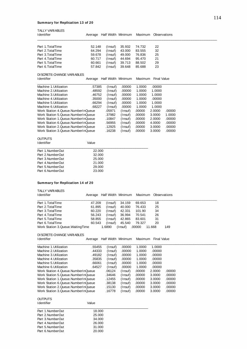
114Summary for Replication 13 of 20 TALLY VARIABLES Identifier Average Half Width Minimum Maximum Observations ___________________________________________________________________________________________________ Part 1.TotalTime 52.148 (Insuf) 35.932 74.732 22 Part 2.TotalTime 64.294 (Insuf) 43.000 83.555 32 Part 3.TotalTime 59.678 (Insuf) 49.000 76.836 25 Part 4.TotalTime 60.717 (Insuf) 44.694 95.470 21 Part 5.TotalTime 60.661 (Insuf) 39.713 88.502 29 Part 6.TotalTime 57.842 (Insuf) 39.648 85.688 23 DISCRETE-CHANGE VARIABLES Identifier Average Half Width Minimum Maximum Final Value ___________________________________________________________________________________________________ Machine 1.Utilization .57385 (Insuf) .00000 1.0000 .00000 Machine 2.Utilization .48592 (Insuf) .00000 1.0000 1.0000 Machine 3.Utilization .46752 (Insuf) .00000 1.0000 1.0000 Machine 4.Utilization .35000 (Insuf) .00000 1.0000 .00000 Machine 5.Utilization .66294 (Insuf) .00000 1.0000 1.0000 Machine 6.Utilization .68227 (Insuf) .00000 1.0000 1.0000 Work Station 4.Queue.NumberInQueue .05971 (Insuf) .00000 2.0000 .00000 Work Station 5.Queue.NumberInQueue .37982 (Insuf) .00000 3.0000 1.0000 Work Station 1.Queue.NumberInQueue .10847 (Insuf) .00000 2.0000 .00000 Work Station 6.Queue.NumberInQueue .56955 (Insuf) .00000 4.0000 .00000 Work Station 2.Queue.NumberInQueue .12925 (Insuf) .00000 3.0000 .00000 Work Station 3.Queue.NumberInQueue .16238 (Insuf) .00000 3.0000 .00000 OUTPUTS Identifier Value _____________________________________________________________ Part 1.NumberOut 22.000 Part 2.NumberOut 32.000 Part 3.NumberOut 25.000 Part 4.NumberOut 21.000 Part 5.NumberOut 29.000 Part 6.NumberOut 23.000 Summary for Replication 14 of 20 TALLY VARIABLES Identifier Average Half Width Minimum Maximum Observations ___________________________________________________________________________________________________ Part 1.TotalTime 47.209 (Insuf) 34.159 69.653 18 Part 2.TotalTime 61.895 (Insuf) 40.000 76.433 25 Part 3.TotalTime 60.220 (Insuf) 42.331 101.90 34 Part 4.TotalTime 56.243 (Insuf) 36.994 70.541 26 Part 5.TotalTime 58.855 (Insuf) 42.865 83.601 31 Part 6.TotalTime 60.543 (Insuf) 45.540 79.327 20 Work Station 3.Queue.WaitingTime 1.6890 (Insuf) .00000 11.668 149 DISCRETE-CHANGE VARIABLES Identifier Average Half Width Minimum Maximum Final Value ___________________________________________________________________________________________________ Machine 1.Utilization .55455 (Insuf) .00000 1.0000 1.0000 Machine 2.Utilization .44333 (Insuf) .00000 1.0000 .00000 Machine 3.Utilization .49182 (Insuf) .00000 1.0000 .00000 Machine 4.Utilization .35835 (Insuf) .00000 1.0000 .00000 Machine 5.Utilization .66061 (Insuf) .00000 1.0000 .00000 Machine 6.Utilization .64527 (Insuf) .00000 1.0000 .00000 Work Station 4.Queue.NumberInQueue .06124 (Insuf) .00000 2.0000 .00000 Work Station 5.Queue.NumberInQueue .34646 (Insuf) .00000 3.0000 .00000 Work Station 1.Queue.NumberInQueue .12455 (Insuf) .00000 3.0000 .00000 Work Station 6.Queue.NumberInQueue .38138 (Insuf) .00000 3.0000 .00000 Work Station 2.Queue.NumberInQueue .15130 (Insuf) .00000 3.0000 .00000 Work Station 3.Queue.NumberInQueue .16778 (Insuf) .00000 3.0000 .00000 OUTPUTS Identifier Value _____________________________________________________________ Part 1.NumberOut 18.000 Part 2.NumberOut 25.000 Part 3.NumberOut 34.000 Part 4.NumberOut 26.000 Part 5.NumberOut 31.000 Part 6.NumberOut 20.000

115Summary for Replication 15 of 20 TALLY VARIABLES Identifier Average Half Width Minimum Maximum Observations ___________________________________________________________________________________________________ Part 1.TotalTime 49.101 (Insuf) 39.172 66.077 16 Part 2.TotalTime 65.030 (Insuf) 49.605 81.797 42 Part 3.TotalTime 64.468 (Insuf) 45.801 88.486 18 Part 4.TotalTime 62.193 (Insuf) 38.995 88.538 21 Part 5.TotalTime 65.019 (Insuf) 45.370 95.045 25 Part 6.TotalTime 63.048 (Insuf) 47.212 85.422 23 DISCRETE-CHANGE VARIABLES Identifier Average Half Width Minimum Maximum Final Value ___________________________________________________________________________________________________ Machine 1.Utilization .58055 (Insuf) .00000 1.0000 1.0000 Machine 2.Utilization .53793 (Insuf) .00000 1.0000 1.0000 Machine 3.Utilization .46046 (Insuf) .00000 1.0000 1.0000 Machine 4.Utilization .34200 (Insuf) .00000 1.0000 .00000 Machine 5.Utilization .67844 (Insuf) .00000 1.0000 1.0000 Machine 6.Utilization .69153 (Insuf) .00000 1.0000 1.0000 Work Station 1.Queue.NumberInQueue .15589 (Insuf) .00000 2.0000 .00000 Work Station 2.Queue.NumberInQueue .20445 (Insuf) .00000 2.0000 1.0000 Work Station 3.Queue.NumberInQueue .21664 (Insuf) .00000 4.0000 .00000 Work Station 4.Queue.NumberInQueue .06792 (Insuf) .00000 2.0000 .00000 Work Station 5.Queue.NumberInQueue .37305 (Insuf) .00000 4.0000 1.0000 Work Station 6.Queue.NumberInQueue .45793 (Insuf) .00000 4.0000 .00000 OUTPUTS Identifier Value _____________________________________________________________ Part 1.NumberOut 16.000 Part 2.NumberOut 42.000 Part 3.NumberOut 18.000 Part 4.NumberOut 21.000 Part 5.NumberOut 25.000 Part 6.NumberOut 23.000 Summary for Replication 16 of 20 TALLY VARIABLES Identifier Average Half Width Minimum Maximum Observations ___________________________________________________________________________________________________ Part 1.TotalTime 46.579 (Insuf) 33.964 66.096 21 Part 2.TotalTime 58.533 (Insuf) 42.000 74.423 15 Part 3.TotalTime 60.049 (Insuf) 43.670 77.689 29 Part 4.TotalTime 58.540 (Insuf) 43.695 84.159 32 Part 5.TotalTime 57.578 (Insuf) 41.914 88.710 26 Part 6.TotalTime 56.166 (Insuf) 38.531 82.596 29 DISCRETE-CHANGE VARIABLES Identifier Average Half Width Minimum Maximum Final Value ___________________________________________________________________________________________________ Machine 1.Utilization .56391 (Insuf) .00000 1.0000 1.0000 Machine 2.Utilization .43064 (Insuf) .00000 1.0000 1.0000 Machine 3.Utilization .44600 (Insuf) .00000 1.0000 .00000 Machine 4.Utilization .33801 (Insuf) .00000 1.0000 1.0000 Machine 5.Utilization .62114 (Insuf) .00000 1.0000 1.0000 Machine 6.Utilization .67650 (Insuf) .00000 1.0000 .00000 Work Station 4.Queue.NumberInQueue .07397 (Insuf) .00000 3.0000 .00000 Work Station 5.Queue.NumberInQueue .20457 (Insuf) .00000 3.0000 .00000 Work Station 1.Queue.NumberInQueue .13635 (Insuf) .00000 2.0000 .00000 Work Station 6.Queue.NumberInQueue .49765 (Insuf) .00000 3.0000 .00000 Work Station 2.Queue.NumberInQueue .10533 (Insuf) .00000 2.0000 1.0000 Work Station 3.Queue.NumberInQueue .20500 (Insuf) .00000 3.0000 .00000 OUTPUTS Identifier Value _____________________________________________________________ Part 1.NumberOut 21.000 Part 2.NumberOut 15.000 Part 3.NumberOut 29.000 Part 4.NumberOut 32.000 Part 5.NumberOut 26.000 Part 6.NumberOut 29.000

116Summary for Replication 17 of 20 TALLY VARIABLES Identifier Average Half Width Minimum Maximum Observations ___________________________________________________________________________________________________ Part 1.TotalTime 48.920 (Insuf) 33.000 61.307 15 Part 2.TotalTime 57.545 (Insuf) 37.000 77.856 22 Part 3.TotalTime 59.689 (Insuf) 42.000 76.166 30 Part 4.TotalTime 55.812 (Insuf) 41.000 76.597 31 Part 5.TotalTime 60.723 (Insuf) 42.586 79.806 31 Part 6.TotalTime 59.850 (Insuf) 38.147 88.150 26 DISCRETE-CHANGE VARIABLES Identifier Average Half Width Minimum Maximum Final Value ___________________________________________________________________________________________________ Machine 1.Utilization .59827 (Insuf) .00000 1.0000 .00000 Machine 2.Utilization .46933 (Insuf) .00000 1.0000 .00000 Machine 3.Utilization .49098 (Insuf) .00000 1.0000 1.0000 Machine 4.Utilization .34267 (Insuf) .00000 1.0000 .00000 Machine 5.Utilization .64787 (Insuf) .00000 1.0000 1.0000 Machine 6.Utilization .70027 (Insuf) .00000 1.0000 .00000 Work Station 4.Queue.NumberInQueue .04890 (Insuf) .00000 2.0000 .00000 Work Station 5.Queue.NumberInQueue .25299 (Insuf) .00000 3.0000 1.0000 Work Station 1.Queue.NumberInQueue .09715 (Insuf) .00000 1.0000 .00000 Work Station 6.Queue.NumberInQueue .47189 (Insuf) .00000 4.0000 .00000 Work Station 2.Queue.NumberInQueue .17042 (Insuf) .00000 3.0000 .00000 Work Station 3.Queue.NumberInQueue .18656 (Insuf) .00000 2.0000 1.0000 OUTPUTS Identifier Value _____________________________________________________________ Part 1.NumberOut 15.000 Part 2.NumberOut 22.000 Part 3.NumberOut 30.000 Part 4.NumberOut 31.000 Part 5.NumberOut 31.000 Part 6.NumberOut 26.000 Summary for Replication 18 of 20 TALLY VARIABLES Identifier Average Half Width Minimum Maximum Observations ___________________________________________________________________________________________________ Part 1.TotalTime 51.183 (Insuf) 36.082 64.323 27 Part 2.TotalTime 60.239 (Insuf) 41.088 88.864 27 Part 3.TotalTime 62.380 (Insuf) 42.709 76.726 29 Part 4.TotalTime 59.870 (Insuf) 43.780 89.059 23 Part 5.TotalTime 60.904 (Insuf) 44.313 94.629 26 Part 6.TotalTime 57.091 (Insuf) 44.000 75.428 23 DISCRETE-CHANGE VARIABLES Identifier Average Half Width Minimum Maximum Final Value ___________________________________________________________________________________________________ Machine 1.Utilization .54759 (Insuf) .00000 1.0000 .00000 Machine 2.Utilization .48672 (Insuf) .00000 1.0000 .00000 Machine 3.Utilization .42000 (Insuf) .00000 1.0000 .00000 Machine 4.Utilization .39914 (Insuf) .00000 1.0000 1.0000 Machine 5.Utilization .65292 (Insuf) .00000 1.0000 .00000 Machine 6.Utilization .65292 (Insuf) .00000 1.0000 .00000 Work Station 4.Queue.NumberInQueue .12875 (Insuf) .00000 3.0000 .00000 Work Station 5.Queue.NumberInQueue .28270 (Insuf) .00000 3.0000 .00000 Work Station 1.Queue.NumberInQueue .13852 (Insuf) .00000 2.0000 .00000 Work Station 6.Queue.NumberInQueue .46506 (Insuf) .00000 3.0000 .00000 Work Station 2.Queue.NumberInQueue .17173 (Insuf) .00000 3.0000 .00000 Work Station 3.Queue.NumberInQueue .11169 (Insuf) .00000 3.0000 .00000 OUTPUTS Identifier Value _____________________________________________________________ Part 1.NumberOut 27.000 Part 2.NumberOut 27.000 Part 3.NumberOut 29.000 Part 4.NumberOut 23.000 Part 5.NumberOut 26.000 Part 6.NumberOut 23.000

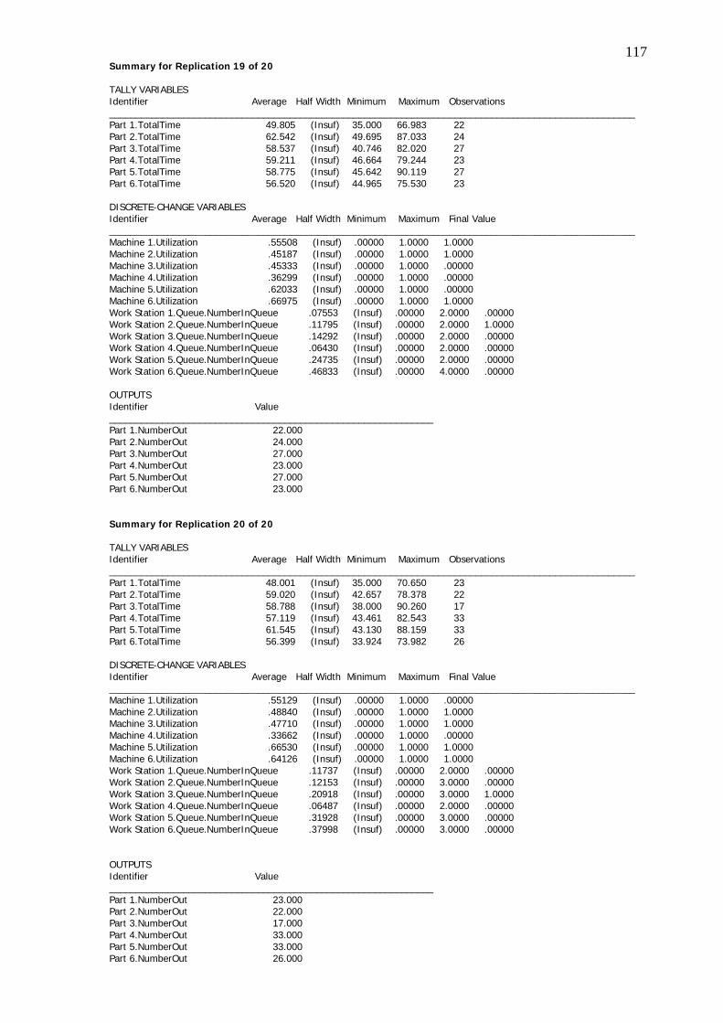
117Summary for Replication 19 of 20 TALLY VARIABLES Identifier Average Half Width Minimum Maximum Observations ___________________________________________________________________________________________________ Part 1.TotalTime 49.805 (Insuf) 35.000 66.983 22 Part 2.TotalTime 62.542 (Insuf) 49.695 87.033 24 Part 3.TotalTime 58.537 (Insuf) 40.746 82.020 27 Part 4.TotalTime 59.211 (Insuf) 46.664 79.244 23 Part 5.TotalTime 58.775 (Insuf) 45.642 90.119 27 Part 6.TotalTime 56.520 (Insuf) 44.965 75.530 23 DISCRETE-CHANGE VARIABLES Identifier Average Half Width Minimum Maximum Final Value ___________________________________________________________________________________________________ Machine 1.Utilization .55508 (Insuf) .00000 1.0000 1.0000 Machine 2.Utilization .45187 (Insuf) .00000 1.0000 1.0000 Machine 3.Utilization .45333 (Insuf) .00000 1.0000 .00000 Machine 4.Utilization .36299 (Insuf) .00000 1.0000 .00000 Machine 5.Utilization .62033 (Insuf) .00000 1.0000 .00000 Machine 6.Utilization .66975 (Insuf) .00000 1.0000 1.0000 Work Station 1.Queue.NumberInQueue .07553 (Insuf) .00000 2.0000 .00000 Work Station 2.Queue.NumberInQueue .11795 (Insuf) .00000 2.0000 1.0000 Work Station 3.Queue.NumberInQueue .14292 (Insuf) .00000 2.0000 .00000 Work Station 4.Queue.NumberInQueue .06430 (Insuf) .00000 2.0000 .00000 Work Station 5.Queue.NumberInQueue .24735 (Insuf) .00000 2.0000 .00000 Work Station 6.Queue.NumberInQueue .46833 (Insuf) .00000 4.0000 .00000 OUTPUTS Identifier Value _____________________________________________________________ Part 1.NumberOut 22.000 Part 2.NumberOut 24.000 Part 3.NumberOut 27.000 Part 4.NumberOut 23.000 Part 5.NumberOut 27.000 Part 6.NumberOut 23.000 Summary for Replication 20 of 20 TALLY VARIABLES Identifier Average Half Width Minimum Maximum Observations ___________________________________________________________________________________________________ Part 1.TotalTime 48.001 (Insuf) 35.000 70.650 23 Part 2.TotalTime 59.020 (Insuf) 42.657 78.378 22 Part 3.TotalTime 58.788 (Insuf) 38.000 90.260 17 Part 4.TotalTime 57.119 (Insuf) 43.461 82.543 33 Part 5.TotalTime 61.545 (Insuf) 43.130 88.159 33 Part 6.TotalTime 56.399 (Insuf) 33.924 73.982 26 DISCRETE-CHANGE VARIABLES Identifier Average Half Width Minimum Maximum Final Value ___________________________________________________________________________________________________ Machine 1.Utilization .55129 (Insuf) .00000 1.0000 .00000 Machine 2.Utilization .48840 (Insuf) .00000 1.0000 1.0000 Machine 3.Utilization .47710 (Insuf) .00000 1.0000 1.0000 Machine 4.Utilization .33662 (Insuf) .00000 1.0000 .00000 Machine 5.Utilization .66530 (Insuf) .00000 1.0000 1.0000 Machine 6.Utilization .64126 (Insuf) .00000 1.0000 1.0000 Work Station 1.Queue.NumberInQueue .11737 (Insuf) .00000 2.0000 .00000 Work Station 2.Queue.NumberInQueue .12153 (Insuf) .00000 3.0000 .00000 Work Station 3.Queue.NumberInQueue .20918 (Insuf) .00000 3.0000 1.0000 Work Station 4.Queue.NumberInQueue .06487 (Insuf) .00000 2.0000 .00000 Work Station 5.Queue.NumberInQueue .31928 (Insuf) .00000 3.0000 .00000 Work Station 6.Queue.NumberInQueue .37998 (Insuf) .00000 3.0000 .00000 OUTPUTS Identifier Value _____________________________________________________________ Part 1.NumberOut 23.000 Part 2.NumberOut 22.000 Part 3.NumberOut 17.000 Part 4.NumberOut 33.000 Part 5.NumberOut 33.000 Part 6.NumberOut 26.000

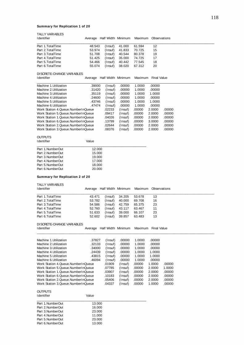
118 Summary for Replication 1 of 20 TALLY VARIABLES Identifier Average Half Width Minimum Maximum Observations ___________________________________________________________________________________________________ Part 1.TotalTime 48.543 (Insuf) 41.000 61.594 12 Part 2.TotalTime 53.974 (Insuf) 41.833 70.725 15 Part 3.TotalTime 51.708 (Insuf) 40.544 80.378 19 Part 4.TotalTime 51.425 (Insuf) 35.000 74.725 17 Part 5.TotalTime 54.466 (Insuf) 40.442 77.545 18 Part 6.TotalTime 55.074 (Insuf) 38.020 67.312 20 DISCRETE-CHANGE VARIABLES Identifier Average Half Width Minimum Maximum Final Value ___________________________________________________________________________________________________ Machine 1.Utilization .39000 (Insuf) .00000 1.0000 .00000 Machine 2.Utilization .31420 (Insuf) .00000 1.0000 .00000 Machine 3.Utilization .35119 (Insuf) .00000 1.0000 1.0000 Machine 4.Utilization .24600 (Insuf) .00000 1.0000 .00000 Machine 5.Utilization .43746 (Insuf) .00000 1.0000 1.0000 Machine 6.Utilization .47474 (Insuf) .00000 1.0000 .00000 Work Station 4.Queue.NumberInQueue .02233 (Insuf) .00000 2.0000 .00000 Work Station 5.Queue.NumberInQueue .09417 (Insuf) .00000 2.0000 .00000 Work Station 1.Queue.NumberInQueue .04026 (Insuf) .00000 2.0000 .00000 Work Station 6.Queue.NumberInQueue .13799 (Insuf) .00000 3.0000 .00000 Work Station 2.Queue.NumberInQueue .02644 (Insuf) .00000 2.0000 .00000 Work Station 3.Queue.NumberInQueue .08376 (Insuf) .00000 2.0000 .00000 OUTPUTS Identifier Value _____________________________________________________________ Part 1.NumberOut 12.000 Part 2.NumberOut 15.000 Part 3.NumberOut 19.000 Part 4.NumberOut 17.000 Part 5.NumberOut 18.000 Part 6.NumberOut 20.000 Summary for Replication 2 of 20 TALLY VARIABLES Identifier Average Half Width Minimum Maximum Observations ___________________________________________________________________________________________________ Part 1.TotalTime 43.471 (Insuf) 34.205 53.678 13 Part 2.TotalTime 53.782 (Insuf) 40.000 69.708 16 Part 3.TotalTime 54.586 (Insuf) 42.759 65.375 23 Part 4.TotalTime 52.760 (Insuf) 43.117 63.467 11 Part 5.TotalTime 51.633 (Insuf) 39.000 66.107 23 Part 6.TotalTime 52.602 (Insuf) 39.857 63.483 13 DISCRETE-CHANGE VARIABLES Identifier Average Half Width Minimum Maximum Final Value ___________________________________________________________________________________________________ Machine 1.Utilization .37827 (Insuf) .00000 1.0000 .00000 Machine 2.Utilization .32133 (Insuf) .00000 1.0000 .00000 Machine 3.Utilization .34000 (Insuf) .00000 1.0000 .00000 Machine 4.Utilization .24439 (Insuf) .00000 1.0000 1.0000 Machine 5.Utilization .43815 (Insuf) .00000 1.0000 1.0000 Machine 6.Utilization .46094 (Insuf) .00000 1.0000 .00000 Work Station 4.Queue.NumberInQueue .01909 (Insuf) .00000 1.0000 .00000 Work Station 5.Queue.NumberInQueue .07785 (Insuf) .00000 2.0000 1.0000 Work Station 1.Queue.NumberInQueue .03907 (Insuf) .00000 2.0000 .00000 Work Station 6.Queue.NumberInQueue .10183 (Insuf) .00000 2.0000 .00000 Work Station 2.Queue.NumberInQueue .05406 (Insuf) .00000 2.0000 .00000 Work Station 3.Queue.NumberInQueue .04337 (Insuf) .00000 1.0000 .00000 OUTPUTS Identifier Value _____________________________________________________________ Part 1.NumberOut 13.000 Part 2.NumberOut 16.000 Part 3.NumberOut 23.000 Part 4.NumberOut 11.000 Part 5.NumberOut 23.000 Part 6.NumberOut 13.000

119Summary for Replication 3 of 20 TALLY VARIABLES Identifier Average Half Width Minimum Maximum Observations ___________________________________________________________________________________________________ Part 1.TotalTime 42.292 (Insuf) 35.602 51.704 13 Part 2.TotalTime 54.754 (Insuf) 41.869 73.876 19 Part 3.TotalTime 54.178 (Insuf) 42.000 70.109 12 Part 4.TotalTime 55.466 (Insuf) 38.000 71.103 15 Part 5.TotalTime 54.972 (Insuf) 41.724 76.140 23 Part 6.TotalTime 56.155 (Insuf) 45.179 70.805 18 DISCRETE-CHANGE VARIABLES Identifier Average Half Width Minimum Maximum Final Value ___________________________________________________________________________________________________ Machine 1.Utilization .40533 (Insuf) .00000 1.0000 .00000 Machine 2.Utilization .34263 (Insuf) .00000 1.0000 1.0000 Machine 3.Utilization .35032 (Insuf) .00000 1.0000 .00000 Machine 4.Utilization .22667 (Insuf) .00000 1.0000 .00000 Machine 5.Utilization .43733 (Insuf) .00000 1.0000 .00000 Machine 6.Utilization .49555 (Insuf) .00000 1.0000 .00000 Work Station 4.Queue.NumberInQueue .01163 (Insuf) .00000 1.0000 .00000 Work Station 5.Queue.NumberInQueue .08179 (Insuf) .00000 2.0000 .00000 Work Station 1.Queue.NumberInQueue .03500 (Insuf) .00000 2.0000 .00000 Work Station 6.Queue.NumberInQueue .14589 (Insuf) .00000 3.0000 .00000 Work Station 2.Queue.NumberInQueue .03024 (Insuf) .00000 1.0000 .00000 Work Station 3.Queue.NumberInQueue .08460 (Insuf) .00000 2.0000 .00000 OUTPUTS Identifier Value _____________________________________________________________ Part 1.NumberOut 13.000 Part 2.NumberOut 19.000 Part 3.NumberOut 12.000 Part 4.NumberOut 15.000 Part 5.NumberOut 23.000 Part 6.NumberOut 18.000 Summary for Replication 4 of 20 TALLY VARIABLES Identifier Average Half Width Minimum Maximum Observations ___________________________________________________________________________________________________ Part 1.TotalTime 42.149 (Insuf) 35.721 59.240 12 Part 2.TotalTime 56.313 (Insuf) 44.000 69.257 17 Part 3.TotalTime 54.428 (Insuf) 44.591 78.107 11 Part 4.TotalTime 49.989 (Insuf) 38.000 79.014 21 Part 5.TotalTime 52.022 (Insuf) 43.000 62.000 31 Part 6.TotalTime 47.344 (Insuf) 43.574 52.399 6 DISCRETE-CHANGE VARIABLES Identifier Average Half Width Minimum Maximum Final Value ___________________________________________________________________________________________________ Machine 1.Utilization .34354 (Insuf) .00000 1.0000 1.0000 Machine 2.Utilization .33200 (Insuf) .00000 1.0000 .00000 Machine 3.Utilization .38828 (Insuf) .00000 1.0000 .00000 Machine 4.Utilization .21989 (Insuf) .00000 1.0000 1.0000 Machine 5.Utilization .45486 (Insuf) .00000 1.0000 .00000 Machine 6.Utilization .43267 (Insuf) .00000 1.0000 .00000 Work Station 1.Queue.NumberInQueue .03092 (Insuf) .00000 2.0000 .00000 Work Station 2.Queue.NumberInQueue .03590 (Insuf) .00000 2.0000 .00000 Work Station 3.Queue.NumberInQueue .04288 (Insuf) .00000 1.0000 .00000 Work Station 4.Queue.NumberInQueue .01646 (Insuf) .00000 1.0000 1.0000 Work Station 5.Queue.NumberInQueue .08696 (Insuf) .00000 2.0000 .00000 Work Station 6.Queue.NumberInQueue .06718 (Insuf) .00000 2.0000 .00000 OUTPUTS Identifier Value _____________________________________________________________ Part 1.NumberOut 12.000 Part 2.NumberOut 17.000 Part 3.NumberOut 11.000 Part 4.NumberOut 21.000 Part 5.NumberOut 31.000 Part 6.NumberOut 6.0000

120Summary for Replication 5 of 20 TALLY VARIABLES Identifier Average Half Width Minimum Maximum Observations ___________________________________________________________________________________________________ Part 1.TotalTime 46.736 (Insuf) 40.000 55.203 13 Part 2.TotalTime 59.746 (Insuf) 44.000 83.202 23 Part 3.TotalTime 56.577 (Insuf) 42.190 95.372 19 Part 4.TotalTime 51.882 (Insuf) 39.000 58.404 20 Part 5.TotalTime 59.083 (Insuf) 43.000 89.884 15 Part 6.TotalTime 51.844 (Insuf) 42.291 70.961 13 DISCRETE-CHANGE VARIABLES Identifier Average Half Width Minimum Maximum Final Value ___________________________________________________________________________________________________ Machine 1.Utilization .39717 (Insuf) .00000 1.0000 1.0000 Machine 2.Utilization .36467 (Insuf) .00000 1.0000 .00000 Machine 3.Utilization .33800 (Insuf) .00000 1.0000 .00000 Machine 4.Utilization .25681 (Insuf) .00000 1.0000 .00000 Machine 5.Utilization .47933 (Insuf) .00000 1.0000 .00000 Machine 6.Utilization .51439 (Insuf) .00000 1.0000 1.0000 Work Station 1.Queue.NumberInQueue .03829 (Insuf) .00000 1.0000 .00000 Work Station 2.Queue.NumberInQueue .06138 (Insuf) .00000 2.0000 .00000 Work Station 3.Queue.NumberInQueue .05142 (Insuf) .00000 1.0000 .00000 Work Station 4.Queue.NumberInQueue .02824 (Insuf) .00000 1.0000 .00000 Work Station 5.Queue.NumberInQueue .11319 (Insuf) .00000 2.0000 .00000 Work Station 6.Queue.NumberInQueue .14575 (Insuf) .00000 3.0000 .00000 OUTPUTS Identifier Value _____________________________________________________________ Part 1.NumberOut 13.000 Part 2.NumberOut 23.000 Part 3.NumberOut 19.000 Part 4.NumberOut 20.000 Part 5.NumberOut 15.000 Part 6.NumberOut 13.000 Summary for Replication 6 of 20 TALLY VARIABLES Identifier Average Half Width Minimum Maximum Observations ___________________________________________________________________________________________________ Part 1.TotalTime 46.840 (Insuf) 36.000 61.090 16 Part 2.TotalTime 52.912 (Insuf) 44.000 74.149 18 Part 3.TotalTime 51.905 (Insuf) 40.081 78.443 13 Part 4.TotalTime 50.142 (Insuf) 39.000 58.000 20 Part 5.TotalTime 52.103 (Insuf) 43.000 67.537 21 Part 6.TotalTime 51.736 (Insuf) 43.000 66.443 13 DISCRETE-CHANGE VARIABLES Identifier Average Half Width Minimum Maximum Final Value ___________________________________________________________________________________________________ Machine 1.Utilization .33533 (Insuf) .00000 1.0000 .00000 Machine 2.Utilization .32284 (Insuf) .00000 1.0000 .00000 Machine 3.Utilization .34785 (Insuf) .00000 1.0000 1.0000 Machine 4.Utilization .25400 (Insuf) .00000 1.0000 .00000 Machine 5.Utilization .45409 (Insuf) .00000 1.0000 .00000 Machine 6.Utilization .45831 (Insuf) .00000 1.0000 1.0000 Work Station 4.Queue.NumberInQueue .02841 (Insuf) .00000 2.0000 .00000 Work Station 5.Queue.NumberInQueue .08647 (Insuf) .00000 1.0000 .00000 Work Station 1.Queue.NumberInQueue .03155 (Insuf) .00000 2.0000 .00000 Work Station 6.Queue.NumberInQueue .08414 (Insuf) .00000 2.0000 .00000 Work Station 2.Queue.NumberInQueue .03741 (Insuf) .00000 2.0000 .00000 Work Station 3.Queue.NumberInQueue .05022 (Insuf) .00000 2.0000 .00000 OUTPUTS Identifier Value _____________________________________________________________ Part 1.NumberOut 16.000 Part 2.NumberOut 18.000 Part 3.NumberOut 13.000 Part 4.NumberOut 20.000 Part 5.NumberOut 21.000 Part 6.NumberOut 13.000

121Summary for Replication 7 of 20 TALLY VARIABLES Identifier Average Half Width Minimum Maximum Observations ___________________________________________________________________________________________________ Part 1.TotalTime 43.443 (Insuf) 35.887 52.523 14 Part 2.TotalTime 57.134 (Insuf) 42.000 68.931 16 Part 3.TotalTime 55.495 (Insuf) 44.653 70.907 17 Part 4.TotalTime 48.484 (Insuf) 39.000 64.679 19 Part 5.TotalTime 52.439 (Insuf) 39.000 69.104 20 Part 6.TotalTime 52.414 (Insuf) 43.177 74.032 16 DISCRETE-CHANGE VARIABLES Identifier Average Half Width Minimum Maximum Final Value ___________________________________________________________________________________________________ Machine 1.Utilization .38000 (Insuf) .00000 1.0000 .00000 Machine 2.Utilization .30924 (Insuf) .00000 1.0000 1.0000 Machine 3.Utilization .34103 (Insuf) .00000 1.0000 .00000 Machine 4.Utilization .25267 (Insuf) .00000 1.0000 .00000 Machine 5.Utilization .44504 (Insuf) .00000 1.0000 .00000 Machine 6.Utilization .46467 (Insuf) .00000 1.0000 .00000 Work Station 4.Queue.NumberInQueue .02548 (Insuf) .00000 1.0000 .00000 Work Station 5.Queue.NumberInQueue .06961 (Insuf) .00000 2.0000 .00000 Work Station 1.Queue.NumberInQueue .04185 (Insuf) .00000 2.0000 .00000 Work Station 6.Queue.NumberInQueue .09441 (Insuf) .00000 2.0000 .00000 Work Station 2.Queue.NumberInQueue .02537 (Insuf) .00000 1.0000 1.0000 Work Station 3.Queue.NumberInQueue .04820 (Insuf) .00000 1.0000 .00000 OUTPUTS Identifier Value _____________________________________________________________ Part 1.NumberOut 14.000 Part 2.NumberOut 16.000 Part 3.NumberOut 17.000 Part 4.NumberOut 19.000 Part 5.NumberOut 20.000 Part 6.NumberOut 16.000 Summary for Replication 8 of 20 TALLY VARIABLES Identifier Average Half Width Minimum Maximum Observations ___________________________________________________________________________________________________ Part 1.TotalTime 44.065 (Insuf) 38.724 50.990 14 Part 2.TotalTime 56.065 (Insuf) 40.000 71.863 13 Part 3.TotalTime 52.623 (Insuf) 42.323 65.143 17 Part 4.TotalTime 51.093 (Insuf) 41.000 67.853 19 Part 5.TotalTime 51.676 (Insuf) 39.000 64.773 17 Part 6.TotalTime 52.471 (Insuf) 38.000 71.564 20 DISCRETE-CHANGE VARIABLES Identifier Average Half Width Minimum Maximum Final Value ___________________________________________________________________________________________________ Machine 1.Utilization .37600 (Insuf) .00000 1.0000 .00000 Machine 2.Utilization .30728 (Insuf) .00000 1.0000 .00000 Machine 3.Utilization .30369 (Insuf) .00000 1.0000 1.0000 Machine 4.Utilization .25891 (Insuf) .00000 1.0000 .00000 Machine 5.Utilization .41887 (Insuf) .00000 1.0000 1.0000 Machine 6.Utilization .50851 (Insuf) .00000 1.0000 1.0000 Work Station 4.Queue.NumberInQueue .02703 (Insuf) .00000 2.0000 .00000 Work Station 5.Queue.NumberInQueue .05953 (Insuf) .00000 1.0000 .00000 Work Station 1.Queue.NumberInQueue .03808 (Insuf) .00000 2.0000 .00000 Work Station 6.Queue.NumberInQueue .12609 (Insuf) .00000 2.0000 .00000 Work Station 2.Queue.NumberInQueue .02076 (Insuf) .00000 1.0000 .00000 Work Station 3.Queue.NumberInQueue .05978 (Insuf) .00000 2.0000 .00000 OUTPUTS Identifier Value _____________________________________________________________ Part 1.NumberOut 14.000 Part 2.NumberOut 13.000 Part 3.NumberOut 17.000 Part 4.NumberOut 19.000 Part 5.NumberOut 17.000 Part 6.NumberOut 20.000

122Summary for Replication 9 of 20 TALLY VARIABLES Identifier Average Half Width Minimum Maximum Observations ___________________________________________________________________________________________________ Part 1.TotalTime 44.743 (Insuf) 34.000 57.046 16 Part 2.TotalTime 55.378 (Insuf) 44.720 65.000 17 Part 3.TotalTime 58.213 (Insuf) 48.889 70.535 14 Part 4.TotalTime 51.248 (Insuf) 43.000 67.124 20 Part 5.TotalTime 52.046 (Insuf) 40.011 83.620 14 Part 6.TotalTime 57.227 (Insuf) 41.485 79.162 17 DISCRETE-CHANGE VARIABLES Identifier Average Half Width Minimum Maximum Final Value ___________________________________________________________________________________________________ Machine 1.Utilization .38133 (Insuf) .00000 1.0000 .00000 Machine 2.Utilization .34068 (Insuf) .00000 1.0000 1.0000 Machine 3.Utilization .32195 (Insuf) .00000 1.0000 1.0000 Machine 4.Utilization .25133 (Insuf) .00000 1.0000 .00000 Machine 5.Utilization .41269 (Insuf) .00000 1.0000 .00000 Machine 6.Utilization .49040 (Insuf) .00000 1.0000 1.0000 Work Station 4.Queue.NumberInQueue .01311 (Insuf) .00000 1.0000 .00000 Work Station 5.Queue.NumberInQueue .07497 (Insuf) .00000 2.0000 .00000 Work Station 1.Queue.NumberInQueue .03333 (Insuf) .00000 1.0000 .00000 Work Station 6.Queue.NumberInQueue .14270 (Insuf) .00000 2.0000 .00000 Work Station 2.Queue.NumberInQueue .05729 (Insuf) .00000 2.0000 .00000 Work Station 3.Queue.NumberInQueue .05181 (Insuf) .00000 2.0000 .00000 OUTPUTS Identifier Value _____________________________________________________________ Part 1.NumberOut 16.000 Part 2.NumberOut 17.000 Part 3.NumberOut 14.000 Part 4.NumberOut 20.000 Part 5.NumberOut 14.000 Part 6.NumberOut 17.000 Summary for Replication 10 of 20 TALLY VARIABLES Identifier Average Half Width Minimum Maximum Observations ___________________________________________________________________________________________________ Part 1.TotalTime 44.609 (Insuf) 34.864 51.930 19 Part 2.TotalTime 55.302 (Insuf) 40.000 78.835 19 Part 3.TotalTime 51.385 (Insuf) 39.804 68.259 20 Part 4.TotalTime 50.883 (Insuf) 41.000 61.283 14 Part 5.TotalTime 59.707 (Insuf) 39.000 79.342 16 Part 6.TotalTime 48.874 (Insuf) 38.551 57.930 12 DISCRETE-CHANGE VARIABLES Identifier Average Half Width Minimum Maximum Final Value ___________________________________________________________________________________________________ Machine 1.Utilization .36241 (Insuf) .00000 1.0000 1.0000 Machine 2.Utilization .34647 (Insuf) .00000 1.0000 1.0000 Machine 3.Utilization .31200 (Insuf) .00000 1.0000 .00000 Machine 4.Utilization .24533 (Insuf) .00000 1.0000 .00000 Machine 5.Utilization .43867 (Insuf) .00000 1.0000 .00000 Machine 6.Utilization .48600 (Insuf) .00000 1.0000 1.0000 Work Station 4.Queue.NumberInQueue .02246 (Insuf) .00000 2.0000 .00000 Work Station 5.Queue.NumberInQueue .07250 (Insuf) .00000 2.0000 .00000 Work Station 1.Queue.NumberInQueue .03327 (Insuf) .00000 2.0000 .00000 Work Station 6.Queue.NumberInQueue .12171 (Insuf) .00000 2.0000 1.0000 Work Station 2.Queue.NumberInQueue .04849 (Insuf) .00000 2.0000 .00000 Work Station 3.Queue.NumberInQueue .02542 (Insuf) .00000 1.0000 .00000 OUTPUTS Identifier Value _____________________________________________________________ Part 1.NumberOut 19.000 Part 2.NumberOut 19.000 Part 3.NumberOut 20.000 Part 4.NumberOut 14.000 Part 5.NumberOut 16.000 Part 6.NumberOut 12.000

123Summary for Replication 11 of 20 TALLY VARIABLES Identifier Average Half Width Minimum Maximum Observations ___________________________________________________________________________________________________ Part 1.TotalTime 45.870 (Insuf) 40.000 52.495 16 Part 2.TotalTime 55.255 (Insuf) 41.869 65.972 17 Part 3.TotalTime 53.547 (Insuf) 38.000 75.815 18 Part 4.TotalTime 52.500 (Insuf) 37.000 66.410 21 Part 5.TotalTime 51.124 (Insuf) 42.808 57.106 13 Part 6.TotalTime 53.724 (Insuf) 37.201 72.349 17 DISCRETE-CHANGE VARIABLES Identifier Average Half Width Minimum Maximum Final Value ___________________________________________________________________________________________________ Machine 1.Utilization .35933 (Insuf) .00000 1.0000 .00000 Machine 2.Utilization .32660 (Insuf) .00000 1.0000 1.0000 Machine 3.Utilization .31281 (Insuf) .00000 1.0000 .00000 Machine 4.Utilization .25733 (Insuf) .00000 1.0000 .00000 Machine 5.Utilization .43614 (Insuf) .00000 1.0000 .00000 Machine 6.Utilization .46943 (Insuf) .00000 1.0000 1.0000 Work Station 4.Queue.NumberInQueue .02103 (Insuf) .00000 1.0000 .00000 Work Station 5.Queue.NumberInQueue .07837 (Insuf) .00000 2.0000 .00000 Work Station 1.Queue.NumberInQueue .04542 (Insuf) .00000 2.0000 .00000 Work Station 6.Queue.NumberInQueue .13448 (Insuf) .00000 2.0000 .00000 Work Station 2.Queue.NumberInQueue .03194 (Insuf) .00000 1.0000 .00000 Work Station 3.Queue.NumberInQueue .03726 (Insuf) .00000 1.0000 .00000 OUTPUTS Identifier Value _____________________________________________________________ Part 1.NumberOut 16.000 Part 2.NumberOut 17.000 Part 3.NumberOut 18.000 Part 4.NumberOut 21.000 Part 5.NumberOut 13.000 Part 6.NumberOut 17.000 Summary for Replication 12 of 20 TALLY VARIABLES Identifier Average Half Width Minimum Maximum Observations ___________________________________________________________________________________________________ Part 1.TotalTime 45.093 (Insuf) 34.000 54.176 11 Part 2.TotalTime 55.347 (Insuf) 44.000 66.726 19 Part 3.TotalTime 53.394 (Insuf) 41.819 69.420 19 Part 4.TotalTime 51.236 (Insuf) 43.000 63.858 14 Part 5.TotalTime 52.649 (Insuf) 39.000 64.106 21 Part 6.TotalTime 55.998 (Insuf) 46.729 63.776 18 DISCRETE-CHANGE VARIABLES Identifier Average Half Width Minimum Maximum Final Value ___________________________________________________________________________________________________ Machine 1.Utilization .41006 (Insuf) .00000 1.0000 1.0000 Machine 2.Utilization .33133 (Insuf) .00000 1.0000 .00000 Machine 3.Utilization .37200 (Insuf) .00000 1.0000 .00000 Machine 4.Utilization .23999 (Insuf) .00000 1.0000 1.0000 Machine 5.Utilization .45134 (Insuf) .00000 1.0000 1.0000 Machine 6.Utilization .48873 (Insuf) .00000 1.0000 1.0000 Work Station 4.Queue.NumberInQueue .01801 (Insuf) .00000 1.0000 .00000 Work Station 5.Queue.NumberInQueue .08041 (Insuf) .00000 2.0000 .00000 Work Station 1.Queue.NumberInQueue .02638 (Insuf) .00000 2.0000 .00000 Work Station 6.Queue.NumberInQueue .12074 (Insuf) .00000 2.0000 .00000 Work Station 2.Queue.NumberInQueue .03427 (Insuf) .00000 2.0000 .00000 Work Station 3.Queue.NumberInQueue .06846 (Insuf) .00000 2.0000 .00000 OUTPUTS Identifier Value _____________________________________________________________ Part 1.NumberOut 11.000 Part 2.NumberOut 19.000 Part 3.NumberOut 19.000 Part 4.NumberOut 14.000 Part 5.NumberOut 21.000 Part 6.NumberOut 18.000

124Summary for Replication 13 of 20 TALLY VARIABLES Identifier Average Half Width Minimum Maximum Observations ___________________________________________________________________________________________________ Part 1.TotalTime 45.816 (Insuf) 34.000 57.480 14 Part 2.TotalTime 56.326 (Insuf) 40.000 76.677 24 Part 3.TotalTime 54.848 (Insuf) 42.234 72.402 17 Part 4.TotalTime 52.772 (Insuf) 46.000 66.438 17 Part 5.TotalTime 53.018 (Insuf) 43.000 72.502 16 Part 6.TotalTime 56.647 (Insuf) 45.809 73.649 13 DISCRETE-CHANGE VARIABLES Identifier Average Half Width Minimum Maximum Final Value ___________________________________________________________________________________________________ Machine 1.Utilization .38480 (Insuf) .00000 1.0000 .00000 Machine 2.Utilization .34340 (Insuf) .00000 1.0000 1.0000 Machine 3.Utilization .32715 (Insuf) .00000 1.0000 1.0000 Machine 4.Utilization .26467 (Insuf) .00000 1.0000 .00000 Machine 5.Utilization .44133 (Insuf) .00000 1.0000 .00000 Machine 6.Utilization .49978 (Insuf) .00000 1.0000 1.0000 Work Station 4.Queue.NumberInQueue .02417 (Insuf) .00000 2.0000 .00000 Work Station 5.Queue.NumberInQueue .09296 (Insuf) .00000 2.0000 .00000 Work Station 1.Queue.NumberInQueue .03393 (Insuf) .00000 2.0000 .00000 Work Station 6.Queue.NumberInQueue .11763 (Insuf) .00000 2.0000 .00000 Work Station 2.Queue.NumberInQueue .02511 (Insuf) .00000 1.0000 .00000 Work Station 3.Queue.NumberInQueue .08304 (Insuf) .00000 3.0000 .00000 OUTPUTS Identifier Value _____________________________________________________________ Part 1.NumberOut 14.000 Part 2.NumberOut 24.000 Part 3.NumberOut 17.000 Part 4.NumberOut 17.000 Part 5.NumberOut 16.000 Part 6.NumberOut 13.000 Summary for Replication 14 of 20 TALLY VARIABLES Identifier Average Half Width Minimum Maximum Observations ___________________________________________________________________________________________________ Part 1.TotalTime 43.020 (Insuf) 35.214 50.325 10 Part 2.TotalTime 56.413 (Insuf) 40.000 71.468 19 Part 3.TotalTime 55.854 (Insuf) 43.021 78.827 22 Part 4.TotalTime 52.771 (Insuf) 43.000 66.191 17 Part 5.TotalTime 53.366 (Insuf) 39.000 66.988 21 Part 6.TotalTime 52.771 (Insuf) 38.159 63.565 13 DISCRETE-CHANGE VARIABLES Identifier Average Half Width Minimum Maximum Final Value ___________________________________________________________________________________________________ Machine 1.Utilization .37467 (Insuf) .00000 1.0000 .00000 Machine 2.Utilization .33000 (Insuf) .00000 1.0000 .00000 Machine 3.Utilization .37261 (Insuf) .00000 1.0000 1.0000 Machine 4.Utilization .23200 (Insuf) .00000 1.0000 .00000 Machine 5.Utilization .45184 (Insuf) .00000 1.0000 .00000 Machine 6.Utilization .51333 (Insuf) .00000 1.0000 .00000 Work Station 1.Queue.NumberInQueue .03259 (Insuf) .00000 2.0000 .00000 Work Station 2.Queue.NumberInQueue .03889 (Insuf) .00000 2.0000 .00000 Work Station 3.Queue.NumberInQueue .06971 (Insuf) .00000 2.0000 .00000 Work Station 4.Queue.NumberInQueue .02176 (Insuf) .00000 2.0000 .00000 Work Station 5.Queue.NumberInQueue .09070 (Insuf) .00000 2.0000 .00000 Work Station 6.Queue.NumberInQueue .12943 (Insuf) .00000 2.0000 .00000 OUTPUTS Identifier Value _____________________________________________________________ Part 1.NumberOut 10.000 Part 2.NumberOut 19.000 Part 3.NumberOut 22.000 Part 4.NumberOut 17.000 Part 5.NumberOut 21.000 Part 6.NumberOut 13.000

125Summary for Replication 15 of 20 TALLY VARIABLES Identifier Average Half Width Minimum Maximum Observations ___________________________________________________________________________________________________ Part 1.TotalTime 44.941 (Insuf) 36.000 51.215 12 Part 2.TotalTime 57.493 (Insuf) 42.000 74.713 27 Part 3.TotalTime 54.500 (Insuf) 44.059 62.346 9 Part 4.TotalTime 51.165 (Insuf) 39.000 64.912 18 Part 5.TotalTime 58.901 (Insuf) 42.000 75.720 15 Part 6.TotalTime 57.448 (Insuf) 41.367 70.292 19 DISCRETE-CHANGE VARIABLES Identifier Average Half Width Minimum Maximum Final Value ___________________________________________________________________________________________________ Machine 1.Utilization .39930 (Insuf) .00000 1.0000 .00000 Machine 2.Utilization .33772 (Insuf) .00000 1.0000 .00000 Machine 3.Utilization .31467 (Insuf) .00000 1.0000 .00000 Machine 4.Utilization .25733 (Insuf) .00000 1.0000 .00000 Machine 5.Utilization .46263 (Insuf) .00000 1.0000 .00000 Machine 6.Utilization .50702 (Insuf) .00000 1.0000 1.0000 Work Station 4.Queue.NumberInQueue .02292 (Insuf) .00000 1.0000 .00000 Work Station 5.Queue.NumberInQueue .11213 (Insuf) .00000 2.0000 .00000 Work Station 1.Queue.NumberInQueue .03578 (Insuf) .00000 2.0000 .00000 Work Station 6.Queue.NumberInQueue .15658 (Insuf) .00000 2.0000 .00000 Work Station 2.Queue.NumberInQueue .01613 (Insuf) .00000 1.0000 .00000 Work Station 3.Queue.NumberInQueue .06775 (Insuf) .00000 2.0000 .00000 OUTPUTS Identifier Value _____________________________________________________________ Part 1.NumberOut 12.000 Part 2.NumberOut 27.000 Part 3.NumberOut 9.0000 Part 4.NumberOut 18.000 Part 5.NumberOut 15.000 Part 6.NumberOut 19.000 Summary for Replication 16 of 20 TALLY VARIABLES Identifier Average Half Width Minimum Maximum Observations ___________________________________________________________________________________________________ Part 1.TotalTime 41.992 (Insuf) 34.000 52.852 16 Part 2.TotalTime 55.347 (Insuf) 44.557 78.018 14 Part 3.TotalTime 51.950 (Insuf) 41.181 76.276 15 Part 4.TotalTime 52.089 (Insuf) 45.861 66.479 16 Part 5.TotalTime 53.664 (Insuf) 44.000 75.000 19 Part 6.TotalTime 53.779 (Insuf) 40.313 67.051 20 DISCRETE-CHANGE VARIABLES Identifier Average Half Width Minimum Maximum Final Value ___________________________________________________________________________________________________ Machine 1.Utilization .36038 (Insuf) .00000 1.0000 1.0000 Machine 2.Utilization .31867 (Insuf) .00000 1.0000 .00000 Machine 3.Utilization .32117 (Insuf) .00000 1.0000 1.0000 Machine 4.Utilization .23800 (Insuf) .00000 1.0000 .00000 Machine 5.Utilization .42657 (Insuf) .00000 1.0000 1.0000 Machine 6.Utilization .47133 (Insuf) .00000 1.0000 .00000 Work Station 4.Queue.NumberInQueue .01166 (Insuf) .00000 1.0000 .00000 Work Station 5.Queue.NumberInQueue .06206 (Insuf) .00000 1.0000 .00000 Work Station 1.Queue.NumberInQueue .04238 (Insuf) .00000 2.0000 .00000 Work Station 6.Queue.NumberInQueue .15366 (Insuf) .00000 2.0000 .00000 Work Station 2.Queue.NumberInQueue .04427 (Insuf) .00000 2.0000 .00000 Work Station 3.Queue.NumberInQueue .06129 (Insuf) .00000 2.0000 .00000 OUTPUTS Identifier Value _____________________________________________________________ Part 1.NumberOut 16.000 Part 2.NumberOut 14.000 Part 3.NumberOut 15.000 Part 4.NumberOut 16.000 Part 5.NumberOut 19.000 Part 6.NumberOut 20.000

126Summary for Replication 17 of 20 TALLY VARIABLES Identifier Average Half Width Minimum Maximum Observations ___________________________________________________________________________________________________ Part 1.TotalTime 47.011 (Insuf) 34.234 63.573 9 Part 2.TotalTime 53.503 (Insuf) 39.562 65.965 14 Part 3.TotalTime 50.816 (Insuf) 39.000 71.377 18 Part 4.TotalTime 51.273 (Insuf) 39.296 61.607 22 Part 5.TotalTime 54.766 (Insuf) 43.126 64.214 21 Part 6.TotalTime 53.550 (Insuf) 42.561 68.697 17 DISCRETE-CHANGE VARIABLES Identifier Average Half Width Minimum Maximum Final Value ___________________________________________________________________________________________________ Machine 1.Utilization .39917 (Insuf) .00000 1.0000 1.0000 Machine 2.Utilization .31915 (Insuf) .00000 1.0000 .00000 Machine 3.Utilization .35318 (Insuf) .00000 1.0000 1.0000 Machine 4.Utilization .22867 (Insuf) .00000 1.0000 .00000 Machine 5.Utilization .43954 (Insuf) .00000 1.0000 1.0000 Machine 6.Utilization .50724 (Insuf) .00000 1.0000 1.0000 Work Station 4.Queue.NumberInQueue .01429 (Insuf) .00000 1.0000 .00000 Work Station 5.Queue.NumberInQueue .07393 (Insuf) .00000 2.0000 .00000 Work Station 1.Queue.NumberInQueue .02814 (Insuf) .00000 2.0000 .00000 Work Station 6.Queue.NumberInQueue .11765 (Insuf) .00000 2.0000 .00000 Work Station 2.Queue.NumberInQueue .04381 (Insuf) .00000 2.0000 .00000 Work Station 3.Queue.NumberInQueue .08176 (Insuf) .00000 3.0000 .00000 OUTPUTS Identifier Value _____________________________________________________________ Part 1.NumberOut 9.0000 Part 2.NumberIn 15.000 Part 2.NumberOut 14.000 Part 3.NumberOut 18.000 Part 4.NumberOut 22.000 Part 5.NumberOut 21.000 Part 6.NumberOut 17.000 Summary for Replication 18 of 20 TALLY VARIABLES Identifier Average Half Width Minimum Maximum Observations ___________________________________________________________________________________________________ Part 1.TotalTime 46.351 (Insuf) 34.000 55.769 15 Part 2.TotalTime 55.154 (Insuf) 44.000 72.506 17 Part 3.TotalTime 51.494 (Insuf) 41.000 64.768 20 Part 4.TotalTime 51.949 (Insuf) 40.292 65.791 18 Part 5.TotalTime 58.042 (Insuf) 39.000 88.603 13 Part 6.TotalTime 52.399 (Insuf) 37.970 67.863 19 DISCRETE-CHANGE VARIABLES Identifier Average Half Width Minimum Maximum Final Value ___________________________________________________________________________________________________ Machine 1.Utilization .38267 (Insuf) .00000 1.0000 .00000 Machine 2.Utilization .32781 (Insuf) .00000 1.0000 1.0000 Machine 3.Utilization .31445 (Insuf) .00000 1.0000 .00000 Machine 4.Utilization .24723 (Insuf) .00000 1.0000 1.0000 Machine 5.Utilization .42778 (Insuf) .00000 1.0000 .00000 Machine 6.Utilization .50333 (Insuf) .00000 1.0000 .00000 Work Station 4.Queue.NumberInQueue .03439 (Insuf) .00000 2.0000 1.0000 Work Station 5.Queue.NumberInQueue .05171 (Insuf) .00000 2.0000 .00000 Work Station 1.Queue.NumberInQueue .03522 (Insuf) .00000 2.0000 .00000 Work Station 6.Queue.NumberInQueue .15524 (Insuf) .00000 3.0000 .00000 Work Station 2.Queue.NumberInQueue .03218 (Insuf) .00000 2.0000 .00000 Work Station 3.Queue.NumberInQueue .07265 (Insuf) .00000 2.0000 .00000 OUTPUTS Identifier Value _____________________________________________________________ Part 1.NumberOut 15.000 Part 2.NumberOut 17.000 Part 3.NumberOut 20.000 Part 4.NumberOut 18.000 Part 5.NumberOut 13.000 Part 6.NumberOut 19.000

127Summary for Replication 19 of 20 TALLY VARIABLES Identifier Average Half Width Minimum Maximum Observations ___________________________________________________________________________________________________ Part 1.TotalTime 46.220 (Insuf) 39.843 56.734 14 Part 2.TotalTime 54.942 (Insuf) 41.808 68.841 17 Part 3.TotalTime 55.836 (Insuf) 44.000 81.003 19 Part 4.TotalTime 48.950 (Insuf) 41.000 65.000 18 Part 5.TotalTime 53.582 (Insuf) 41.328 85.879 17 Part 6.TotalTime 57.288 (Insuf) 40.542 69.656 14 DISCRETE-CHANGE VARIABLES Identifier Average Half Width Minimum Maximum Final Value ___________________________________________________________________________________________________ Machine 1.Utilization .36133 (Insuf) .00000 1.0000 .00000 Machine 2.Utilization .33733 (Insuf) .00000 1.0000 .00000 Machine 3.Utilization .32708 (Insuf) .00000 1.0000 1.0000 Machine 4.Utilization .24267 (Insuf) .00000 1.0000 .00000 Machine 5.Utilization .44643 (Insuf) .00000 1.0000 1.0000 Machine 6.Utilization .48400 (Insuf) .00000 1.0000 .00000 Work Station 4.Queue.NumberInQueue .02639 (Insuf) .00000 2.0000 .00000 Work Station 5.Queue.NumberInQueue .08527 (Insuf) .00000 2.0000 .00000 Work Station 1.Queue.NumberInQueue .02836 (Insuf) .00000 2.0000 .00000 Work Station 6.Queue.NumberInQueue .10419 (Insuf) .00000 2.0000 .00000 Work Station 2.Queue.NumberInQueue .04778 (Insuf) .00000 1.0000 .00000 Work Station 3.Queue.NumberInQueue .08249 (Insuf) .00000 2.0000 .00000 OUTPUTS Identifier Value _____________________________________________________________ Part 1.NumberOut 14.000 Part 2.NumberOut 17.000 Part 3.NumberOut 19.000 Part 4.NumberOut 18.000 Part 5.NumberOut 17.000 Part 6.NumberOut 14.000 Summary for Replication 20 of 20 TALLY VARIABLES Identifier Average Half Width Minimum Maximum Observations ___________________________________________________________________________________________________ Part 1.TotalTime 43.856 (Insuf) 33.349 54.384 15 Part 2.TotalTime 54.351 (Insuf) 45.000 60.594 15 Part 3.TotalTime 51.816 (Insuf) 43.000 72.026 13 Part 4.TotalTime 50.888 (Insuf) 39.000 77.076 22 Part 5.TotalTime 53.095 (Insuf) 44.800 68.046 21 Part 6.TotalTime 54.813 (Insuf) 43.829 74.311 14 DISCRETE-CHANGE VARIABLES Identifier Average Half Width Minimum Maximum Final Value ___________________________________________________________________________________________________ Machine 1.Utilization .33594 (Insuf) .00000 1.0000 1.0000 Machine 2.Utilization .33400 (Insuf) .00000 1.0000 .00000 Machine 3.Utilization .33800 (Insuf) .00000 1.0000 .00000 Machine 4.Utilization .24867 (Insuf) .00000 1.0000 .00000 Machine 5.Utilization .44803 (Insuf) .00000 1.0000 1.0000 Machine 6.Utilization .45667 (Insuf) .00000 1.0000 .00000 Work Station 4.Queue.NumberInQueue .02776 (Insuf) .00000 1.0000 .00000 Work Station 5.Queue.NumberInQueue .06092 (Insuf) .00000 1.0000 1.0000 Work Station 1.Queue.NumberInQueue .02392 (Insuf) .00000 1.0000 .00000 Work Station 6.Queue.NumberInQueue .10219 (Insuf) .00000 2.0000 .00000 Work Station 2.Queue.NumberInQueue .04409 (Insuf) .00000 2.0000 .00000 Work Station 3.Queue.NumberInQueue .07656 (Insuf) .00000 2.0000 .00000 OUTPUTS Identifier Value _____________________________________________________________ Part 1.NumberOut 15.000 Part 2.NumberOut 15.000 Part 3.NumberOut 13.000 Part 4.NumberOut 22.000 Part 5.NumberOut 21.000 Part 6.NumberOut 14.000

APPENDIX D

Example of Summary for Result from Simulation

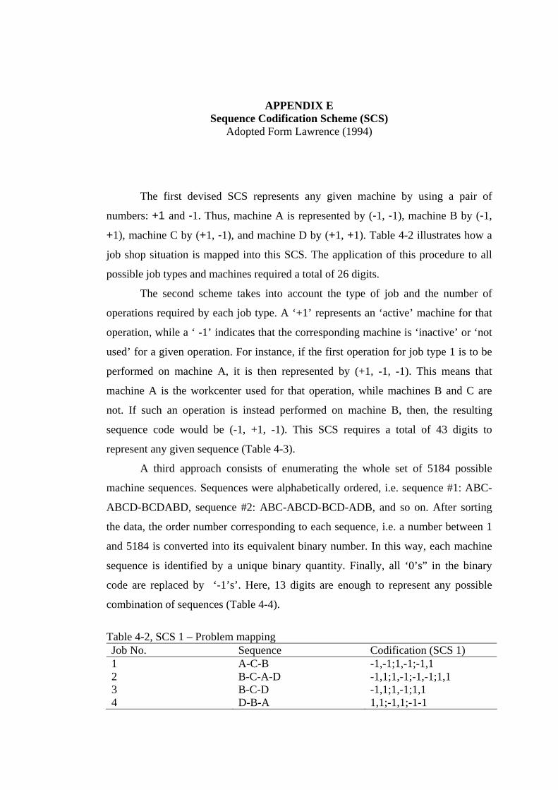
APPENDIX E Sequence Codification Scheme (SCS)

Adopted Form Lawrence (1994)

The first devised SCS represents any given machine by using a pair of

numbers: +1 and -1. Thus, machine A is represented by (-1, -1), machine B by (-1,

+1), machine C by (+1, -1), and machine D by (+1, +1). Table 4-2 illustrates how a

job shop situation is mapped into this SCS. The application of this procedure to all

possible job types and machines required a total of 26 digits.

The second scheme takes into account the type of job and the number of

operations required by each job type. A ‘+1’ represents an ‘active’ machine for that

operation, while a ‘ -1’ indicates that the corresponding machine is ‘inactive’ or ‘not

used’ for a given operation. For instance, if the first operation for job type 1 is to be

performed on machine A, it is then represented by (+1, -1, -1). This means that

machine A is the workcenter used for that operation, while machines B and C are

not. If such an operation is instead performed on machine B, then, the resulting

sequence code would be (-1, +1, -1). This SCS requires a total of 43 digits to

represent any given sequence (Table 4-3).

A third approach consists of enumerating the whole set of 5184 possible

machine sequences. Sequences were alphabetically ordered, i.e. sequence #1: ABC-

ABCD-BCDABD, sequence #2: ABC-ABCD-BCD-ADB, and so on. After sorting

the data, the order number corresponding to each sequence, i.e. a number between 1

and 5184 is converted into its equivalent binary number. In this way, each machine

sequence is identified by a unique binary quantity. Finally, all ‘0’s” in the binary

code are replaced by ‘-1’s’. Here, 13 digits are enough to represent any possible

combination of sequences (Table 4-4).

Table 4-2, SCS 1 – Problem mapping Job No. Sequence Codification (SCS 1) 1 2 3 4

A-C-B B-C-A-D B-C-D D-B-A

-1,-1;1,-1;-1,1 -1,1;1,-1;-1,-1;1,1 -1,1;1,-1;1,1 1,1;-1,1;-1-1

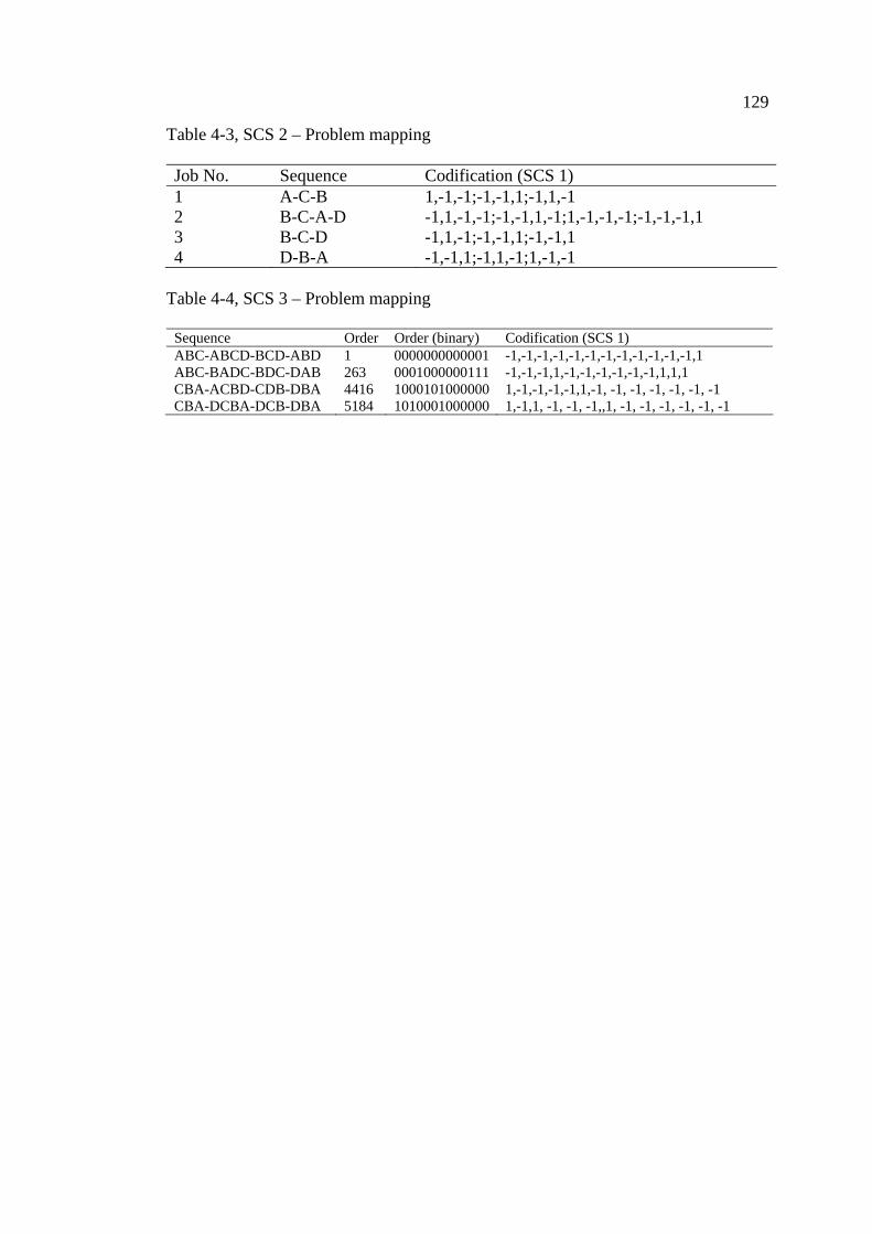
129

Table 4-3, SCS 2 – Problem mapping

Job No. Sequence Codification (SCS 1) 1 2 3 4

A-C-B B-C-A-D B-C-D D-B-A

1,-1,-1;-1,-1,1;-1,1,-1 -1,1,-1,-1;-1,-1,1,-1;1,-1,-1,-1;-1,-1,-1,1 -1,1,-1;-1,-1,1;-1,-1,1 -1,-1,1;-1,1,-1;1,-1,-1

Table 4-4, SCS 3 – Problem mapping

Sequence Order Order (binary) Codification (SCS 1) ABC-ABCD-BCD-ABD ABC-BADC-BDC-DAB CBA-ACBD-CDB-DBA CBA-DCBA-DCB-DBA

1 263 4416 5184

0000000000001 0001000000111 1000101000000 1010001000000

-1,-1,-1,-1,-1,-1,-1,-1,-1,-1,-1,-1,1 -1,-1,-1,1,-1,-1,-1,-1,-1,-1,1,1,1 1,-1,-1,-1,-1,1,-1, -1, -1, -1, -1, -1, -1 1,-1,1, -1, -1, -1,,1, -1, -1, -1, -1, -1, -1