LAND COVER AND TEMPERATURE IMPLICATIONS FOR THE … · 2018-03-28 · e.g. groundwater and surface hydrology, agriculture and orchards, desertification in the dry grassland areas

Geographia Technica, Vol. 13, Issue 1, 2018, pp 85 to 108

LAND COVER AND TEMPERATURE IMPLICATIONS FOR THE

SEASONAL EVAPOTRANSPIRATION IN EUROPE

Mărgărit-Mircea NISTOR1*, Titus Cristian MAN2, Mostafa Ali BENZAGHTA3,

Nikhil NEDUMPALLILE VASU4, Ştefan DEZSI2, Richard KIZZA1

DOI: 10.21163/GT_2018.131.09

ABSTRACT:

Land cover and spatial variation of seasonal temperature may contribute to different

evapotranspiration rates between the European regions. In order to assess the integral effect

of land cover and climate on water resources, we implemented a procedure which allows

defining favorability areas to high rate of evapotranspiration. Seasonal mean air temperature

for the present (2011-2040) and future (2041-2070) combined with the seasonal crop

coefficients of current future projections of land cover for the 2040s have been used to

evaluate the various degrees of evapotranspiration at European scale. Extremely high and

very high degree of evapotranspiration tendency were verified for Southern, Eastern,

Western and Central of Europe during the mid-season period. The low and very low

evapotranspiration favorability were found in the Scandinavian Peninsula and in the Alps,

Dinarics, and Carpathian during the present period in all the seasons. In the cold season, the

land cover favorability to evapotranspiration (LCFE) is low and very low in almost the

whole Europe. These findings indicate that the southern and western regions of Europe are

facing low water availability, decrease in surface water flow, and possible long periods of

drought in the summers.

Key-words: Crop coefficients, Climate change, Evapotranspiration favorability, Europe.

1. INTRODUCTION

Europe is a dynamic continent from many points of view. Changes in land cover

pattern after the 1980s and urban development were observed continuously in many

locations, especially around the capitals and larger cities. Natural places, such as mountain

areas and the wetlands indicate a low degree of urbanization, but at the same time, these

regions are facing global natural changes. The climate is warming (Haeberli et al, 1999;

IPCC, 2001) and most of the glaciers and ice lands have been retreating continuously in the

last decades (Kargel et al, 2005; Oerlemans, 2005; Shahgedanova et al, 2005; Dong et al,

2013; Xie et al, 2013; Elfarrak et al, 2014; Nistor & Petcu, 2015). The main variations at

1Nanyang Technological University, School of Civil and Environmental Engineering, 639798,

Singapore; *Corresponding author email: [email protected]; Last co-author email: [email protected] 2Faculty of Geography, University of Babeş-Bolyai, 400006, Cluj-Napoca, Romania, emails:

[email protected], [email protected] 3Soil and Water Department, Faculty of Agriculture, Sirte University, 054, Sirte, Libya, email:

[email protected] 4British Geological Survey, Keyworth, Nottinghamshire, NG125GG, UK. email: [email protected]

http://dx.doi.org/10.21163/GT_2018.131.09

86

global and continental scales come from changes in the mean air temperature which are

expected to increase for the mid-century. Moreover, the natural systems are often

influenced by climate change (Parmesan & Yohe, 2003; Aguilera & Murillo, 2009; Yustres

et al, 2013; Jiménez Cisneros et al, 2014; Kløve et al, 2014). The most affected resources

by climate change are the water resources, both freshwater and groundwater (Loàiciga et al,

2000; Bachu & Adams, 2003; Brouyère et al, 2004; Campos et al, 2013; Nistor et al, 2014;

Prăvălie et al, 2014). The ecosystems are also facing climate change in many places from

the globe, with significant changes in the biodiversity composition as well (Nistor, 2013;

Nistor & Petcu, 2014).

In the last decades, climate change effects on water resources were claimed in details

through numerous examples, regarding water quality and water quantity (Jiménez Cisneros

et al, 2014). More than this, the climate change impact together with the land cover

contributes to the hydrologic sensitivity of an area. Öztürk et al (2013) modelled the impact

of land use on rural watershed from northern Turkey, mentioning that the hydrological

processes influence watersheds with respect to meteorology, surfaces and underground

characteristics. Thus, land cover represents a crucial factor in evapotranspiration, runoff,

infiltration, and groundwater recharge (Öztürk et al, 2013). The runoff and

evapotranspiration have been studied by Čenčur Curk et al (2014) in South-East Europe for

groundwater vulnerability. Cheval et al (2017) used regional coupled models in the

determination of aridity in South-Eastern Europe. In their survey, climate change and land

cover have been carefully studied and several areas with high vulnerability were depicted,

especially in locations with less water availability, aquifers characteristics, and pollution

load index of each land cover type. Thus, an important role of surface and groundwater

resources come from the evapotranspiration phenomena, which shows an essential concern

for water balance and water surplus (Li et al, 2007; Rosenberry et al, 2007; Gowda et al,

2008). At the temperate zone, climate and land cover are directly responsible for

evapotranspiration, a fact for which many investigations on this topic have been carried out

in recent years by Ambas & Baltas (2012), Nistor & Porumb-Ghiurco (2015), Nistor et al

(2016a), Nistor et al (2016b), Nistor et al (2017a), Nistor et al (2017b). They applied an

original method, which assesses crop evapotranspiration at regional scale based on seasonal

potential evapotranspiration, and standard seasonal crop coefficients (Kc) presented in the

FAO Paper no. 56 (Allen et al, 1998; Allen, 2000). Considering this methodology, changes

of climate and land cover could be problematic for many natural systems of the regions,

e.g. groundwater and surface hydrology, agriculture and orchards, desertification in the dry

grassland areas. Nistor (2016) determined the seasonal Kc for the Paris metropolitan area.

In the Kingdom of Saudi Arabia, Güçlü et al (2017) calculated evapotranspiration using a

regional fuzzy chain model. Based on the REMO and ALADIN regional climate models,

Ladányi et al (2015) analyzed the drought hazard in south-central Hungary, in the

Kiskunság National Park. Gao et al (2007) estimated the actual evapotranspiration over

China during 1961-2002. The spatial-temporal characteristics of the actual

evapotranspiration have been completed by Gao et al (2012) in the Haihe River basin from

East China.

Regarding heterogeneity of the European continent and the current climate change,

significant changes in the climate parameters such as temperature, rainfall, and

evapotranspiration are expected for the mid-century. Considering the land cover projections

for Europe, different visions over the economy, agriculture, industry, and natural

ecosystems may be drawn. A method, which combines mean air temperature and land cover

Mărgărit-Mircea NISTOR, Titus Cristian MAN, Mostafa Ali BENZAGHTA, Nikhil … 87

87

to evaluate the synergy of climate and vegetation pattern on evapotranspiration parameter,

could be a new issue for Europe, from many points of view.

The scope of the present paper is to propose a methodology to assess the effect of

seasonal temperature and seasonal Kc on evapotranspiration following the spatial-temporal

scale of Europe during 2011-2070. The second scope is to identify the favorability areas

with different degrees for the evapotranspiration. Our results contribute both to the

specialty literature of Europe and may be useful to policymakers for decision making

regarding agricultural management and environmental planning.

2. STUDY AREA

The analyzed territory in this paper includes the Western, Northern, Southern, and

Central regions of Europe. To these lands are added the British Islands and some islands

from the Mediterranean Sea, e.g. Sardinia, Corsica, Aegean Islands, Baleares Islands. The

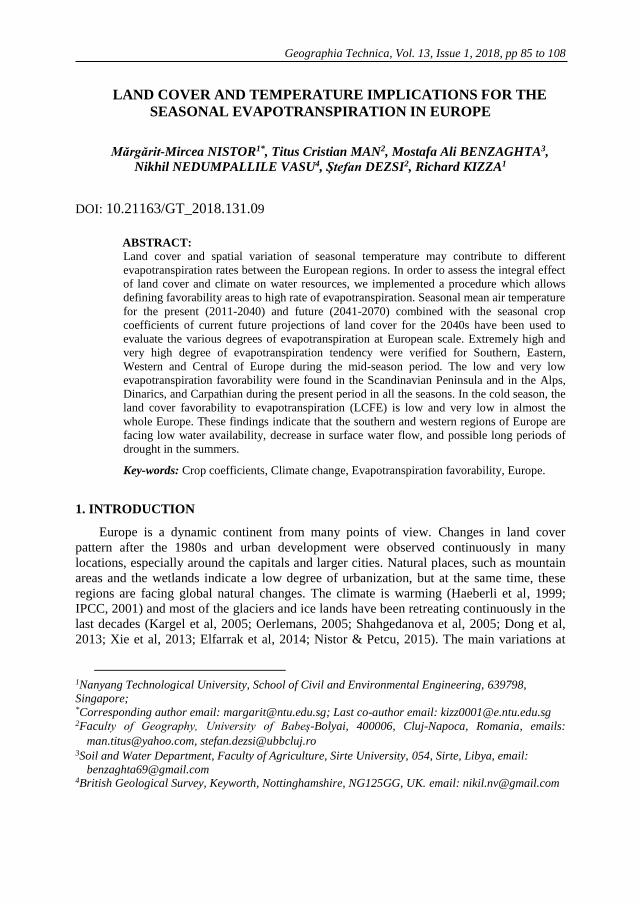
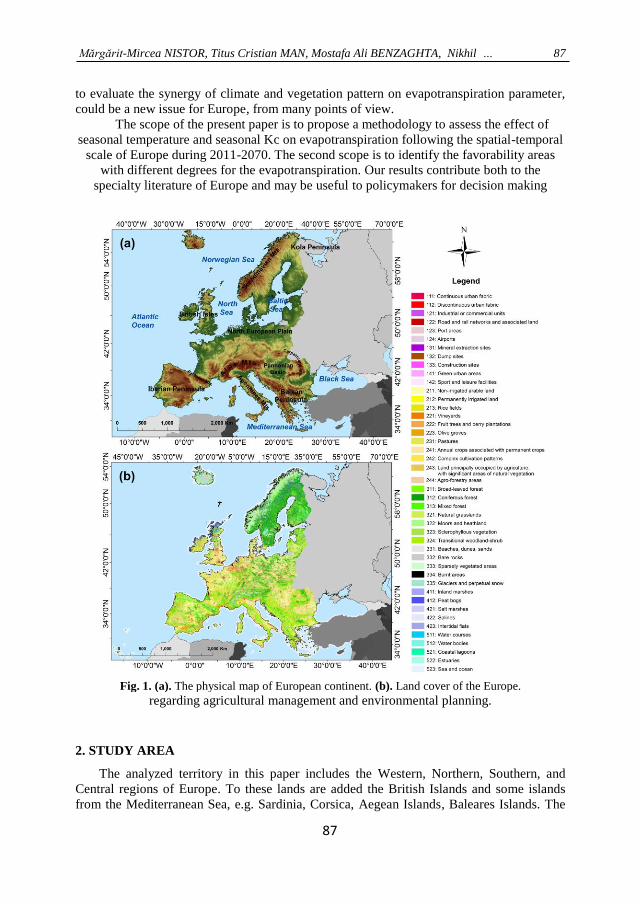
Fig. 1. (a). The physical map of European continent. (b). Land cover of the Europe.

88

eastern sides of the continent, such as Russian, Ukraine, and Belarus have not been

investigated here due to lack of land cover data. For future projections, Switzerland,

Norway, and countries from the West of Balkan Peninsula do not have already completed

land cover patterns. For Iceland, climate data are absent. The morphology of Europe

indicates numerous landforms in correspondence with the main reliefs that are found in the

territory (Fig. 1a). The highlands of the continent consist mainly of mountain chains: Alps

Range, Carpathian Range, Dinarics Mountains, Pyrenees Mountains, Scandinavian

Mountains and Apennines Mountains. The lowlands overlap to the North European Plain,

Pannonian basin, South of British Islands, Romanian Plain, Po Plain. Between mountains

and plains, hilly and plateau reliefs could be found. The coastline of Europe shows very

articulated promontories, sea bays, fjords, and islands.

The geographical position, in the northern hemisphere between 34°35’ to 80°42’

latitude N and 8°59’ longitude W to 66°42’ longitude E and the presence of the Atlantic

Ocean in the West are the main factors which influence the climate of Europe. Thus, in the

North, there is more of a Baltic climate, while in the South, the Saharan and Mediterranean

influences are felt. The western side of Europe together with the British Islands have more

oceanic influences and in the eastern parts, the continentality is more presented. The relief

arrangement and the regional wind movements induce local climate such as mountain

climate, Pontic influence near the Black Sea and the transition climate between oceanic and

continental could be identified in the East-central parts. The mean air temperature range

from -12 °C to 21 °C and the maximum mean precipitation reaches 3500 mm year-1.

According to the Köppen-Geiger climate classification, the Cfa climate characterized by

hot summers and a fully humid period was depicted in the Central, North-central, Southern,

and Southeastern sides (Kottek et al, 2006). In the Scandinavian Peninsula and in the

northeastern extremities, the Dfc class (cool climate) has been observed. The eastern and

southeastern areas of Europe have Dfa and Dfb climates, which implies a cool climate but

with hot and warm summers. The Csb climate was identified in the North of the Iberian

Peninsula while in the South of the Iberian Peninsula, the Csa climate was depicted (Kottek

et al, 2006). The high mountains and in the Scandinavian territory, the tundra climate is

presented due to low temperatures (Kottek et al, 2006).

According to relief and climate, the vegetation of Europe is very diversified (Fig. 1b).

The plains and hilly areas are favorable for agricultural lands, herbaceous vegetation, and

grasslands. In the mountain areas up to 1800 m altitude, there extends the coniferous

vegetation. Broad-leaved and mixed forests grow both in the mountains and hilly areas. The

main species of trees that can be found in Europe include the oak (Quercus), elms (Ulmus),

beech (Fagus), and hornbeam (Carpinus) (European Environment Agency, 2007).

Transnational woodland, shrubs and pasture predominantly cover the elevated areas (over

1800 m). The coastal areas are often covered by green vegetation of various types of trees

and sclerophyllous vegetation. Deltas, lagoons, and marshes are specifically for the low

coastal areas such as Rhone Delta, Po Delta, and Danube Delta. European coastlines do not

miss artificial port areas, man-made infrastructure and dams.

3. MATERIALS AND METHODS

3.1. Climate data

In order to determine the seasonal temperature of Europe at a spatial scale, we used the

climate models of temperature for 30 years related to 2011 to 2040 (present) and 2041-2070

(future). Andreas Hamann, from Alberta University, Canada, constructed these climate


89

models at a very high resolution using the ANUSplin interpolation method. The mean

monthly air temperature served to complete the raster datasets for four seasons according to

the seasonal periods in the temperate zone but also in relationship with the growth plant

calendar in Europe. The climate models were carried out based on the historical data from

1901 to 2013 followed the Mitchell & Jones (2005) method.

The ClimateEU v4.63 software package has been used to complete the climate models.

The CMIP5 multi-model dataset, related to the IPCC Assessment Report 5 (2013) have

been considered for the future projections. Representative Concentration Pathway (RCP)

4.5 by +1.4°C (±0.5) for the 2050s was used due to the global warming mean projections.

The methodology of the models is exposed in a clear way by Hamann & Wang (2005),

Daly et al. (2006), Mbogga et al (2009), and Hamann et al (2013). For the present study,

the climate models spatial resolution was set at 1 km2.

Fig. 2. Land cover projections of Europe. (a) Scenario A1. (b) Scenario A2. (c) Scenario B1. (d)

Scenario B2. Source: Sustainable futures for Europe’s HERitage in CULtural landscapES”

project (http://www.hercules-landscapes.eu/).

3.2. Land cover data

90

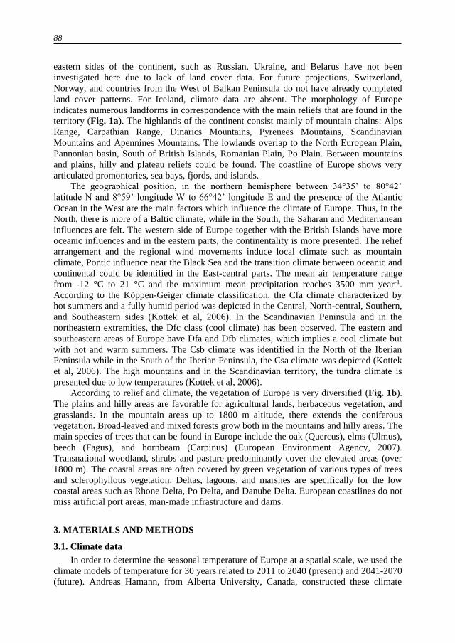
CORINE Land Cover raster data from 2012 at 250 m2 spatial resolution have been

used to identify the main crops, shrubs and trees, and the land use in Europe. We agree with

the CORINE Land Cover due to its georeferenced characteristics and the detailed classes up

to 4th level.

Table 1. Corine Land Cover classes and representative seasonal Kc coefficients in Europe during the present

period.

Corine Land Cover Kc ini

season

Kc mid

season

Kc end

season

Kc cold

season

CLC code 2012

CLC Description Kclc Kclc Kclc Kclc

111 Continous urban fabric 0.2 0.4 0.25 -

112 Discontinuous urban fabric 0.1 0.3 0.2 -

121 Industrial or commercial units 0.2 0.4 0.3 -

122 Road and rail networks and associated land 0.15 0.35 0.25 -

123 Port areas 0.3 0.5 0.4 -

124 Airports 0.2 0.4 0.3 -

131 Mineral extraction sites 0.16 0.36 0.26 -

132 Dump sites 0.16 0.36 0.26 -

133 Construction sites 0.16 0.36 0.26 -

141 Green urban areas 0.12 0.32 0.22 -

142 Sport and leisure facilities 0.1 0.3 0.2 -

211 Non-irrigated arable land 1.1 1.35 1.25 -

212 Permanently irrigated land 1.2 1.45 1.35 -

213 Rice fields 1.05 1.2 0.6 -

221 Vineyards 0.3 0.7 0.45 -

222 Fruit trees and berry plantations 0.3 1.05 0.5 -

223 Olive groves 0.65 0.7 0.65 0.5

231 Pastures 0.4 0.9 0.8 -

241 Annual crops associated with permanent crops 0.5 0.8 0.7 -

242 Complex cultivation patterns 1.1 1.35 1.25 -

243 Land principally occupied by agriculture, with significant areas of natural vegetation

0.7 1.15 1 -

244 Agro-forestry areas 0.9 1.1 1.05 0.3

Source: From Allen et al. (1998); Nistor and Porumb-Ghiurco (2015); Nistor (2017); Nistor et al. (2017)


91

This database is available on Copernicus Land Monitoring Services (2012) website. The

projections of future land cover for the main European countries were carried out in the

“Sustainable futures for Europe’s HERitage in CULtural landscapES” (Hercules) project,

GA no. 603447 (Schulp et al, 2015). The Hercules models offer a spatial vision of the land

cover dynamics based on the fourteen trajectories in the land cover trend. These trajectories

incorporate the macro-economic and land use modes taking into account urbanization,

agriculture, and forestry. The “Landscape Character Index”, extracted from various

landscapes such as land use intensity, structures, and patterns (Schulp et al, 2015) was

considered during mapping of the future land cover. In the present paper, we used the

projections of A1, A2, B1, and B2 land cover scenarios for the 2040s, which illustrate

sixteen classes of land types (Fig. 2). Access to these scenarios could be done through the

Hercules website (http://www.hercules-landscapes.eu/). Entire procedure to obtain the land

cover models is exposed in Report no. 1 of the Hercules project (Schulp et al, 2015). All

Table 1. Corine Land Cover classes and representative seasonal Kc coefficients in Europe during the

present period (continue).

Corine Land Cover Kc ini season

Kc mid season

Kc end season

Kc cold season

CLC code

2012 CLC Description Kclc Kclc Kclc Kclc

311 Broad-leaved forest 1.3 1.6 1.5 0.6

312 Coniferous forest 1 1 1 1

313 Mixed forest 1.2 1.5 1.3 0.8

321 Natural grasslands 0.3 1.15 1.1 -

322 Moors and heathland 0.8 1 0.95 -

323 Sclerophyllous vegetation 0.25 0.9 0.8 -

324 Transitional woodland-shrub 0.8 1 0.95 -

331 Beaches, dunes, sands 0.2 0.3 0.25 -

332 Bare rocks 0.15 0.2 0.05 -

333 Sparsely vegetated areas 0.4 0.6 0.5 -

334 Burnt area 0.1 0.15 0.05 -

335 Glaciers and perpetual snow 0.48 0.52 0.52 0.48

411 Inland marshes 0.15 0.45 0.8 -

412 Peat bogs 0.1 0.4 0.75 -

421 Salt marshes 0.1 0.3 0.7 -

422 Salines 0.1 0.15 0.05 -

423 Intertidal flats 0.3 0.7 1.3 -

511 Water courses 0.25 0.65 1.25 -

512 Water bodies 0.25 0.65 1.25 -

521 Coastal lagoons 0.3 0.7 1.3 -

522 Estuaries 0.25 0.65 1.25 -

523 Sea and ocean 0.4 0.8 1.4 -


92

maps were set at 1 X 1 km to be in line with the climate models resolution. The ArcGIS

environment was used for this investigation due to its reliability in spatial analysis of

territory (Chaieb et al, 2017; Nistor & Petcu, 2015).

3.3. Seasonal crop coefficients (Kc)

Each vegetation type has an evapotranspiration capacity called Kc. In order to calculate

the crop evapotranspiration, Allen et al (1998) used the methodology based on standard Kc.

These coefficients have been calculated both for single and dual crops, at different latitudes

and in different climate types. According to Allen et al (1998), we set the seasonal Kc for

the four seasons specific in the temperate zone. In the urban areas and bare soils,

Grimmond & Oke (1999) completed the Kc in several cities and locations from the United

States. In the European regions, such as Pannonian basin and South East Europe, Nistor et

al (2017a) and Nistor et al (2017b) analyzed crop evapotranspiration at spatial scale

incorporating climate models and land cover data. They provided the Kc values for

CORINE land cover classes and they explained the time shifts for the four seasons in their

study area.

Here, we adopted the above methodology to assess the Kc values both for the present

land cover and for the future. We agree with four seasons like initial season (Kc ini) during

March, April and May, the mid-season (Kc mid) during June, July and August, the end

season (Kc end) during September and October, and the cold season (Kc cold) during January,

February, November, and December. These periods were set first by Nistor & Porumb-

Ghiurco (2015) who proposed the regional methodology at regional scale for Emilia-

Romagna region. Further, Nistor et al (2016b) applied the same procedure for the

Carpathian region. The stages, periods and the standard Kc values may slightly vary from

place to place, with respect to latitude and local climate.

Table 1 reports the seasonal values of Kc used in this paper for the present period

while Table 2 illustrates the kc values for the projected land cover scenarios.

0 - 2 0.21 - 0.6 0.61 - 0.8 0.81 - 1 1.01 - 1.3 > 1.3

Very low Low Medium High Very high Extremely high

Very cool ˂ 0 Very low Very low Very low Very low Very low Very low Very low

Cool 0 - 4 Low Very low Low Low Medium Medium Medium

Temperate 5 - 10. Medium Low Low Medium Medium High High

Warm 11 - 15. High Low Medium Medium High Very high Very high

Hot 16 - 20. Very high Medium Medium High Very high Very high Extremely high

Very hot > 20 Extremely high High High Very high Very high Extremely high Extremely high

Very low Low Medium High Very high Extremely high

Temperature [° C]

Crop coefficient

Susceptibility degree for evapotranspiration

Susceptibility

degree

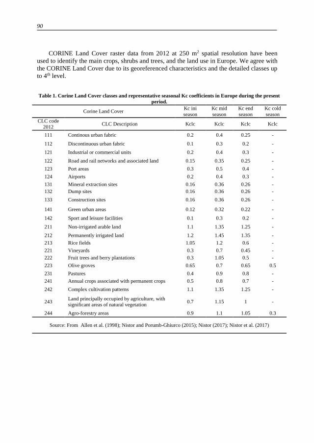
Fig. 3. The inference matrix used to assess the LCFE in Europe.


93

3.4. NISTOR–LCFE method for assessing the land cover favorability for

evapotranspiration

The goal of the survey is to assess the seasonal temperature and seasonal Kc for

Europe and to determine a method, which defines the areas with different degrees of

evapotranspiration favorability. New Implemented Spatial-Temporal On Regions–Land

Cover Favorability to Evapotranspiration (NISTOR-LCFE) method has been set to map

favorability areas to evapotranspiration, and accounting for both the seasonal mean air

temperature and seasonal Kc values. NISTOR–LCFE approach is a new tool based on 6 × 6

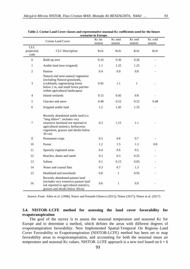
Table 2. Corine Land Cover classes and representative seasonal Kc coefficients used for the future

scenarios in Europe.

Corine Land Cover Kc ini season

Kc mid season

Kc end season

Kc cold season

CLC

projection

code

CLC Description Kclc Kclc Kclc Kclc

0 Built-up area 0.16 0.36 0.26 -

1 Arable land (non-irrigated) 1.1 1.35 1.25 -

2 Pasture 0.4 0.9 0.8 -

3

Natural and semi-natural vegetation

(including Natural grasslands,

scrublands, regenerating forest below 2 m, and small forest patches

within agricultural landscapes)

0.45 1.1 1 -

4 Inland wetlands 0.15 0.45 0.8 -

5 Glaciers and snow 0.48 0.52 0.52 0.48

6 Irrigated arable land 1.2 1.45 1.35 -

7

Recently abandoned arable land (i.e. “long fallow”; includes very

extensive farmland not reported in

agricultural statistics, herbaceous vegetation, grasses and shrubs below

30 cm)

0.3 1.15 1.1 -

8 Permanent crops 0.5 0.8 0.7 -

10 Forest 1.2 1.5 1.3 0.8

11 Sparsely vegetated areas 0.4 0.6 0.5 -

12 Beaches, dunes and sands 0.2 0.3 0.25 -

13 Salines 0.1 0.15 0.05 -

14 Water and coastal flats 0.3 0.7 1.3 -

15 Heathland and moorlands 0.8 1 0.95 -

16

Recently abandoned pasture land

(includes very extensive pasture land not reported in agricultural statistics,

grasses and shrubs below 30cm)

0.6 1 0.9 -


94

matrix that provides six degrees of favorability and it is easy to implement at spatial-

temporal scale. Nistor et al (2016a), Nistor & Mîndrescu (2017) have used an appropriate

survey by matrix application in the hydrology study. Firstly, we classify the

evapotranspiration favorability based on temperature and Kc values in six-degree classes:

very low, low, medium, high, very high, and extremely high. The classification was done

according to previous studies and observed thresholds of seasonal temperature and Kc

values that may influence the evapotranspiration phenomena. We agree with the matrix

classification due to climate and hydrological processes that may occur at different

temperatures, in various types of vegetation cover. Figure 3 shows the proposed matrix

used in the present methodology.

4. RESULTS

The seasonal mean air temperature and seasonal Kc have been completed for Europe in

two time shifts (present and future) on the basis of the presented methodology. Figure 4

depicts the seasonal temperature in Europe for the 2011-2040 and 2041-2070 according to

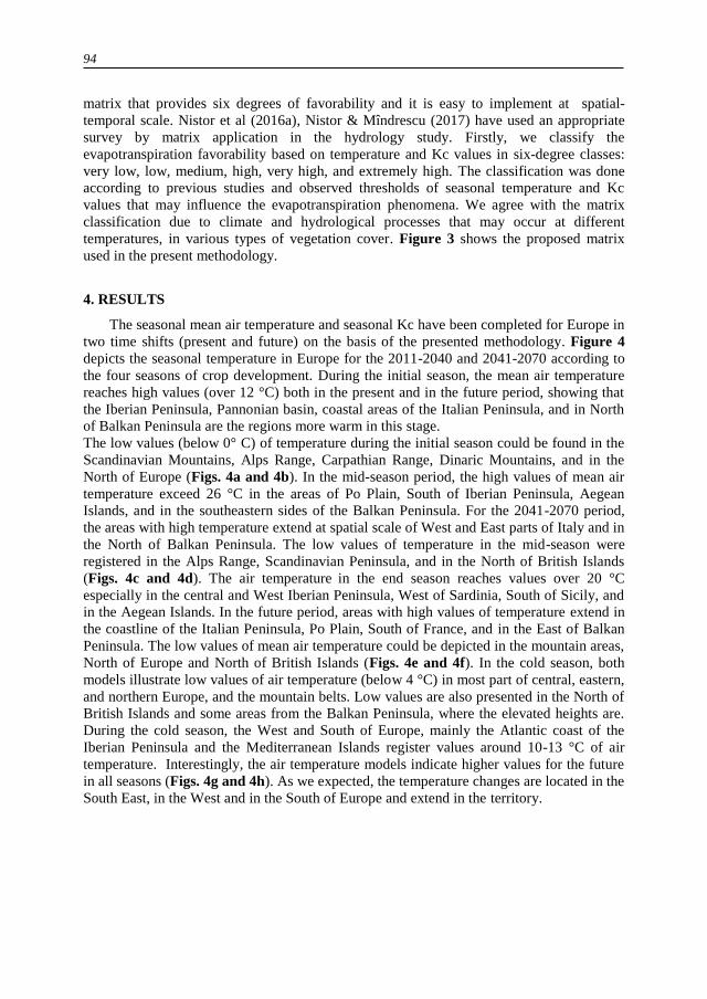
the four seasons of crop development. During the initial season, the mean air temperature

reaches high values (over 12 °C) both in the present and in the future period, showing that

the Iberian Peninsula, Pannonian basin, coastal areas of the Italian Peninsula, and in North

of Balkan Peninsula are the regions more warm in this stage.

The low values (below 0° C) of temperature during the initial season could be found in the

Scandinavian Mountains, Alps Range, Carpathian Range, Dinaric Mountains, and in the

North of Europe (Figs. 4a and 4b). In the mid-season period, the high values of mean air

temperature exceed 26 °C in the areas of Po Plain, South of Iberian Peninsula, Aegean

Islands, and in the southeastern sides of the Balkan Peninsula. For the 2041-2070 period,

the areas with high temperature extend at spatial scale of West and East parts of Italy and in

the North of Balkan Peninsula. The low values of temperature in the mid-season were

registered in the Alps Range, Scandinavian Peninsula, and in the North of British Islands

(Figs. 4c and 4d). The air temperature in the end season reaches values over 20 °C

especially in the central and West Iberian Peninsula, West of Sardinia, South of Sicily, and

in the Aegean Islands. In the future period, areas with high values of temperature extend in

the coastline of the Italian Peninsula, Po Plain, South of France, and in the East of Balkan

Peninsula. The low values of mean air temperature could be depicted in the mountain areas,

North of Europe and North of British Islands (Figs. 4e and 4f). In the cold season, both

models illustrate low values of air temperature (below 4 °C) in most part of central, eastern,

and northern Europe, and the mountain belts. Low values are also presented in the North of

British Islands and some areas from the Balkan Peninsula, where the elevated heights are.

During the cold season, the West and South of Europe, mainly the Atlantic coast of the

Iberian Peninsula and the Mediterranean Islands register values around 10-13 °C of air

temperature. Interestingly, the air temperature models indicate higher values for the future

in all seasons (Figs. 4g and 4h). As we expected, the temperature changes are located in the

South East, in the West and in the South of Europe and extend in the territory.


95

Fig. 4. Spatial distribution of seasonal air temperature in Europe. (a) Temperature for the initial (ini)

season (2011 – 2040). (b) Temperature for the initial (ini) season (2041 – 2070). (c) Temperature for

the mid-season (mid) (2011 – 2040). (d) Temperature for the mid-season (mid) (2041 – 2070). (e)

Temperature for the end season (2011 – 2040). (f) Temperature for the end season (2041 – 2070). (f)

Temperature for the cold season (2011 – 2040). (h) Temperature for the cold season (2041 – 2070).

96

Fig. 6. Spatial distribution of Kc in Europe related to the projection of scenario A1. (a) Kc ini for the

initial season. (b) Kc mid for the mid-season season. (c) Kc end for the end season. (d) Kc cold for the

cold season.

Fig. 5. Spatial distribution of Kc in Europe related to the present land cover. (a) Kc ini for the

initial season. (b) Kc mid for the mid-season season. (c) Kc end for the end season. (d) Kc cold

for the cold season.


97

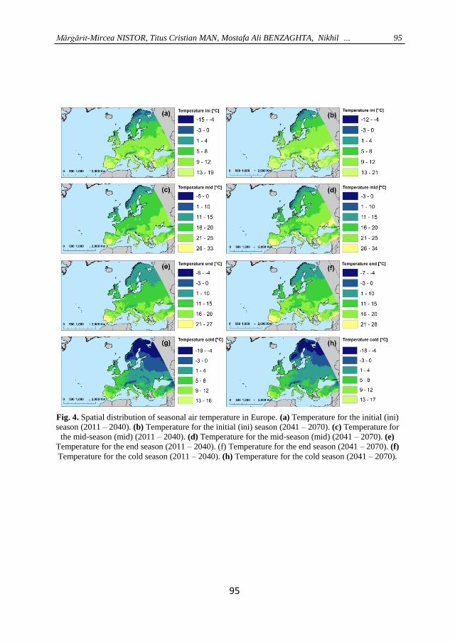
During the present period, the Kc values range from 0 to 1.6 and register the maximum

values in the mid-season stage (Fig. 5). The high values (1.31-1.6) could be depicted in the

central, West, South-East, and South parts of Europe. The lower values of the Kc are

related to the cold season when major parts of the continent have Kc values that range from

0 to 0.3. During the initial and end seasons, the Kc values reach 1.3 and 1.5 respectively

and mean Kc indicates values around 0.81-1. The future land Kc illustrates values between

0 and 1.5, the maximum values being assigned for the mid-season stage. The cold season

shows values up to 0.8 and the larger sides of the Europe have values of Kc between 0 and

0.48. Differences in the Kc pattern for the future are illustrated in Figures 6-9.

The LCFE map shows high and very high degree of favorability for the initial season

in the East, South, and West sides of Europe, especially in the lowlands and on the coastal

areas. The medium degree spread mainly in the Scandinavian Peninsula, Carpathian

Mountains, Eastern Alps, central sides of the Europe, and in South of Iberian Peninsula.

The low and very low LCFE were depicted in the North of Europe, North and West of the

British Islands and in the mountain areas, especially in the Alps Range, Pyrenees, Central

Apennines, and Dinaric Mountains. In the future period, increase in high degree has been

observed in the Scandinavian Peninsula and in eastern Europe. The medium class of LCFE

increases also for all scenarios in the Iberian Peninsula and in South of Europe, e.g. Sicily

Island, Aegean Islands, South of Balkan Peninsula. Figure 10 illustrates the favorability

degree in Europe related to the initial season.

Fig. 7. Spatial distribution of Kc in Europe related to the projection of scenario A2. (a) Kc ini for the

initial season. (b) Kc mid for the mid-season season. (c) Kc end for the end season. (d) Kc cold for

the cold season.

98

Fig. 8. Spatial distribution of Kc in Europe related to the projection of scenario B1. (a) Kc ini for the

initial season. (b) Kc mid for the mid-season season. (c) Kc end for the end season. (d) Kc cold for

the cold season.

Fig. 9. Spatial distribution of Kc in Europe related to the projection of scenario B2. (a) Kc ini for the

initial season. (b) Kc mid for the mid-season season. (c) Kc end for the end season. (d) Kc cold for the

cold season.


99

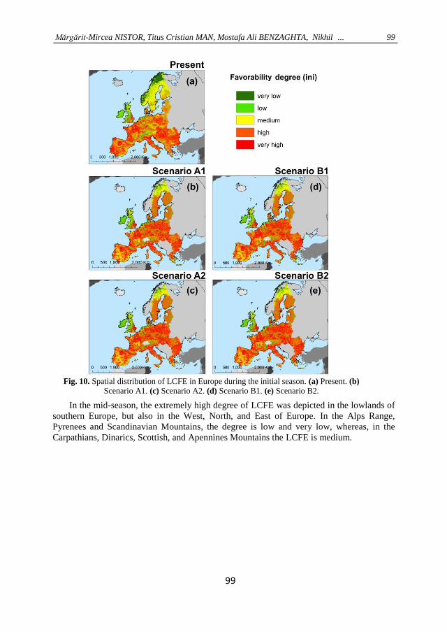
In the mid-season, the extremely high degree of LCFE was depicted in the lowlands of

southern Europe, but also in the West, North, and East of Europe. In the Alps Range,

Pyrenees and Scandinavian Mountains, the degree is low and very low, whereas, in the

Carpathians, Dinarics, Scottish, and Apennines Mountains the LCFE is medium.

Fig. 10. Spatial distribution of LCFE in Europe during the initial season. (a) Present. (b)

Scenario A1. (c) Scenario A2. (d) Scenario B1. (e) Scenario B2.

100

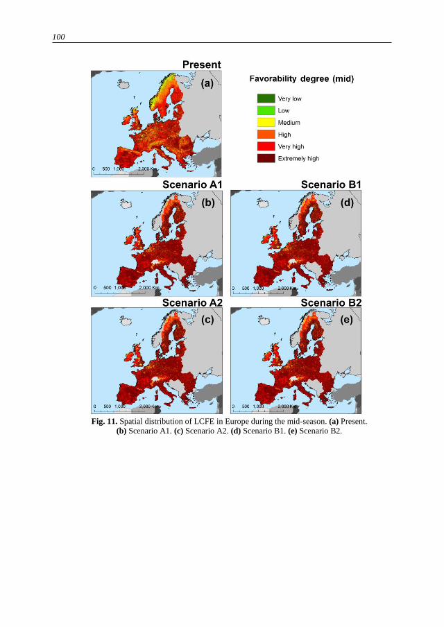
Fig. 11. Spatial distribution of LCFE in Europe during the mid-season. (a) Present.

(b) Scenario A1. (c) Scenario A2. (d) Scenario B1. (e) Scenario B2.


101

The medium LCFE was found also in the large capitals and cities, e.g. London, Paris,

Birmingham, and in the central and western sides of the Scandinavian Peninsula. The future

scenarios indicate largest areas with an extremely high degree of the LCFE in the central,

South, West, and some eastern sides of the Europe. Figure 11 depicts the favorability

degree in Europe related to the mid-season.

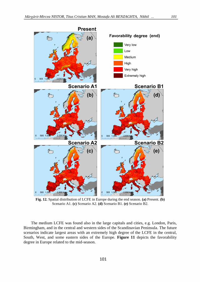
Fig. 12. Spatial distribution of LCFE in Europe during the end season. (a) Present. (b)

Scenario A1. (c) Scenario A2. (d) Scenario B1. (e) Scenario B2.

102

During the end season, the present LCFE map illustrates large areas with high and very

high degree for evapotranspiration favorability, while the extremely high LCFE was

depicted mainly in the West of Iberian Peninsula, South of Balkan Peninsula, Italian

Peninsula, in some places from central Europe, and in the Mediterranean Islands. Medium,

low, and very low degree were identified in the Alps Range, Scandinavian Peninsula, North

of British Islands, Pyrenees Mountains, East of Sicily and in the Etna Mount. The medium

LCFE extends also in the large urban areas, and in the central Iberian Peninsula, South of

France, sparsely in the central and East of Europe. The future scenarios show increase of

areas with extremely high degree of evapotranspiration favorability, especially in the

southern, western, and eastern sides of Europe. The favorability degree in the end season of

Europe is presented in Figure 12.

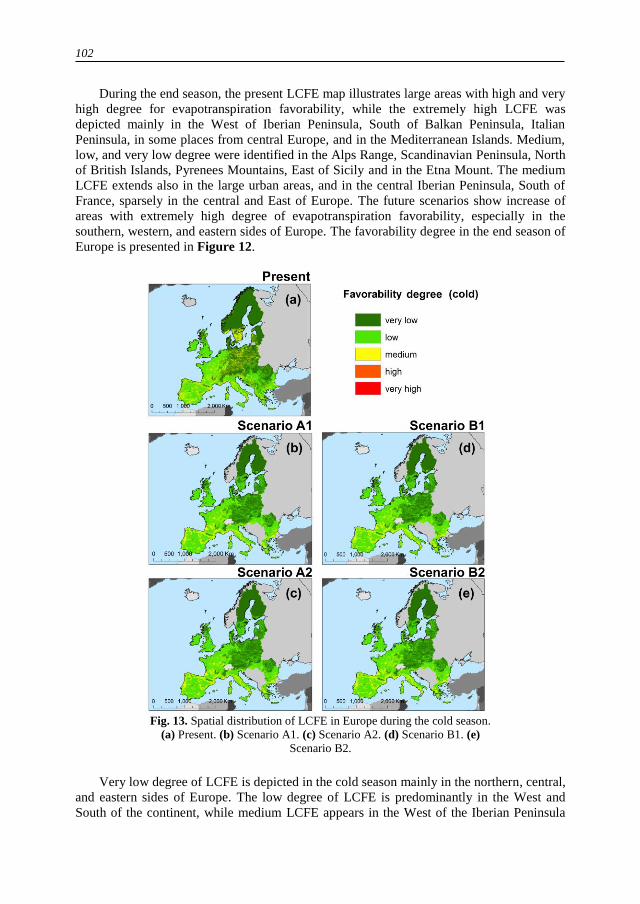
Very low degree of LCFE is depicted in the cold season mainly in the northern, central,

and eastern sides of Europe. The low degree of LCFE is predominantly in the West and

South of the continent, while medium LCFE appears in the West of the Iberian Peninsula

Fig. 13. Spatial distribution of LCFE in Europe during the cold season.

(a) Present. (b) Scenario A1. (c) Scenario A2. (d) Scenario B1. (e)

Scenario B2.


103

and sparsely in central and northern Europe, in Italian and Balkan Peninsula. This degree

class extends also in the South of the Scandinavian Peninsula, but only for the present

period. The future scenarios show an increase of low and very low degree in the East and

North of Europe, whereas in the West and South of Europe, the medium class increases in

the spatial distribution. A remarkable situation about high and very high degree of LCFE

could be found only for the present in few locations from South of Italy, South of Balkan

Peninsula, around the coastal areas of the Iberian Peninsula, and in the Aegean Islands.

Figure 13 depicts the favorability degree in Europe related to the cold season.

5. DISCUSSION

The main goal of this paper is to evaluate the seasonal mean air temperature and the

seasonal Kc in Europe during 2011-2040 and 2041-2070 and to implement a methodology

to identify areas with different degrees of favorability to evapotranspiration. The

seasonality in Europe and, in general, in the temperate zone indicates four stages with

various characteristics in the climate regime and growth of plants. As a parameter which

indicates the exchange between vegetation and atmosphere (Chen et al, 2006), the

evapotranspiration parameter is a useful indicator in hydrological and climate studies. First

and the most important input for the evapotranspiration calculation is temperature because,

without positive values of temperature, lack of energy as a result cannot produce

evapotranspiration. Spatial distribution of seasonal mean air temperature is very diversified

in Europe, with significant influences of Atlantic Ocean in the West and Mediterranean

influences in the South sides, where temperatures are higher than in central, eastern and

northern Europe. On the Eastern sides, North of the Black Sea, the high values of seasonal

temperature are present also. These higher values of temperature were found in all seasons.

A slight increase for the future period (2041-2070) could be observed. Continentality and

large parts of land in eastern Europe contribute to the low and negative temperature in the

cold season. The North of Europe is influenced by the Arctic cool zone, a fact for which the

values of temperature are lower than in other parts of Europe, especially in the cold and

initial season. As a consequence of the distribution of temperature in the European territory,

evapotranspiration rate highly correlates to the quantity of heat and sunshine energy. For

this reason, the southern and western regions of Europe are more susceptible to high

evapotranspiration.

Land cover composition is the second factor which affects evapotranspiration, due to

different absorption and hydrological exchanges of various vegetation types, and because of

the crop calendar. In this sense, the non-vegetative land cover features such as glaciers,

urban areas, or bare soil, contribute to evapotranspiration rate much in the mid-season

period. In the northern lands of Europe and in the North of British Islands, low values of Kc

are observed due to peat bogs areas, heath and moorlands fields. In the mountain areas,

glaciers and coniferous forests influence the Kc. The ice covers have values of 0.48 (initial

and cold season) and 0.52 (mid-season and end season), especially in the Alps, and the

evergreen areas and the coniferous forest have a value 1 in all seasons. This is important

because the evapotranspiration expectation could be higher also during the winter.

The future seasonal Kc does not reach the maximum value such as in the present due to

simplified classes of the land cover. Thus, the forest class is not differentiated in the future

by the broad-leaved and mixed forests, so one unique class for this type was used for the

projections of land cover. The artificial areas are also represented only by one class, which

104

included all built-up areas. Due to these simplifications, the future spatial distribution of Kc

that resulted from the scenarios indicate values lower than in the present up to 0.15 in the

end season, but the Kc values are still within the range of previous literature studies.

Analyzing the seasonal Kc patterns, it was observed that in the A1 scenario, lands with

higher Kc are larger than in scenario B1 during all seasons. Comparing scenario A2 with

scenario B2, areas with high Kc occupies more territory in scenario B2 than in scenario A2.

From the analysis of scenario A1 and scenario B2, it was concluded that scenario A1 has

more territory with high values of Kc in comparison with B2 scenario. The last, between

scenarios A2 and B1, the analysis of patterns indicates larger areas with high Kc in scenario

A2 than in scenario B1.

Incorporating the seasonal temperature and seasonal Kc of Europe in the 6 × 6 matrix

as the NISTOR-LCFE method proposes, the favorability degree to evapotranspiration is

highly dependent on the spatial distribution of both variables. The extremely high and very

high LSCE is predominantly in the mid-season because mean air temperature is high in this

season and also vegetation functions are more active than in other seasons. LCFE with very

high and extremely high favorability was identified in the initial and end season, while in

the cold season, the low and very low LCFE are predominant in Europe. In response to

climate change, the future LCFE maps illustrate major changes in the high and very high

degree class of favorability.

Even if we do not calculate crop evapotranspiration, the findings carried out through

the NISTOR-LCFE method may be compared to the results obtained by Nistor & Porumb-

Ghiurco (2015), Nistor et al (2016b), Nistor et al (2017a), Nistor et al (2017b) which assess

the crop evapotranspiration in different regions of Europe. The above mentioned studies

indicate high values of evapotranspiration during the mid-season, with an increase of areas

with high and very high crop evapotranspiration. However, the key work of Nistor (2016)

related to seasonal Kc in the Paris metropolitan area represented the base for Kc values

decision for this paper.

Our work is not without limitations, considering that the complicated hydrological

processes related to evapotranspiration are very complex. Here, we presented a reliable

methodology to assess the LCFE at European scale. Based on climate models to extract

seasonal temperature and using land cover database to determine the spatial distribution of

Kc, the results could be slightly different at the local scale due to missing field

measurements of Kc. The large territory of Europe and the multitude of land cover types do

not permit us to complete an exhaustive survey using tensiometers and lysimeters. For this

reason, we admit to using standard Kc knowing that evapotranspiration rate may fluctuate

under the coefficients of evapotranspiration.

6. CONCLUSIONS

Spatial distribution of seasonal mean air temperature and seasonal Kc have been

mapped for Europe in two time shifts with an aim to depict different degrees of

evapotranspiration favorability using a new spatial-temporal approach. The application of

the NISTOR-LCFE method combines climate models and land cover data in an efficient

way that can be easily completed in ArcGIS environment. The power of our original

method offers an overall view at spatial scale of favorability areas to evapotranspiration

without the necessity to execute potential evapotranspiration which requires time and

calculations. In addition, the NISTOR-LCFE approach has not been used in previous

researches and this outcome may contribute to the specific literature.


105

The areas from West, South, and East Europe are susceptible to very high and

extremely high degree of evapotranspiration during the mid-season and in the future, these

areas would seem to extend. For the same season, the low and very low LCFE overlap to

the mountain belts and on the northern territory. The medium LCFE is mainly presented in

the initial season and spread over the northern sides of Europe, in the Iberian Peninsula,

South of Europe, West-central parts of Europe (e.g. in France), and in the Carpathians

Mountains. For an optimization of numerous environmental factors and for good practices

in the society for decision making, our maps could be helpful to indicate drought areas

during the summer periods, runoff and water surplus calculations, and to set up agricultural

management planning.

Our findings fit also with climatology and hydrological sciences, for which further

calculations of potential and actual evapotranspiration concerning groundwater

vulnerability could be drawn. In this sense, the utilization of climate models and land cover

scenarios are an exciting issue for many expertise fields. Future works will focus on water

resources quantitative statement under climate change linking also land cover implications.

To support the planning for environmental management, we provide out gridded data layers

of seasonal temperature and seasonal Kc through an open access database

(https://zenodo.org: 10.5281/zenodo.1193226).

Acknowledgements

The authors would like to thank Andreas Hamann from Alberta University for the

climate model data, European Environmental Agency and Hercules team members for the

land cover raster data. Previous affiliation of the corresponding author: Earthresearch

Company, Department of Hydrogeology, Cluj-Napoca, Romania.

REFERENCES

Aguilera, H. & Murillo, J.M. (2009) The effect of possible climate change on natural groundwater

recharge based on a simple model: a study of four karstic aquifers in SE Spain. Environmental

Geology, 57(5), 963–974.

Allen, R.G., Pereira, L.S., Raes, D. & Smith, M. (1998) Crop Evapotranspiration: Guidelines for

Computing Crop Water Requirements. FAO Irrigation and Drainage Paper 56. FAO: Rome, pp.

300.

Allen, R.G. (2000) Using the FAO-56 dual crop coefficient method over an irrigated region as part of

an evapotranspiration intercomparison study. Journal of Hydrology, 229, 27–41.

Ambas, V.T. & Baltas, E. (2012) Sensitivity analysis of different evapotranspiration methods using a

new sensitivity coefficient. Global NEST Journal, 14(3), 335–343.

Bachu, S. & Adams, J.J. (2003) Sequestration of CO2 in geological media in response to climate

change: capacity of deep saline aquifers to sequester CO2 in solution. Energy Conversion and

Management, 44, 3151–3175.

Brouyère, S., Carabin, G. & Dassargues, A. (2004) Climate change impacts on groundwater resources:

modelled deficits in a chalky aquifer, Geer basin, Belgium. Hydrogeology Journal, 12, 123–134.

Campos, G.E.P., Moran, M.S., Huete, A., Zhang, Y., Bresloff, C., Huxman, T.E. et al. (2013)

Ecosystem resilience despite large-scale altered hydroclimatic conditions. Nature, 494, 349–353.

Čenčur Curk, B., Cheval, S., Vrhovnik, P., Verbovšek, T., Herrnegger, M., Nachtnebel, H.P.,

Marjanović, P., Siegel, H., Gerhardt, E., Hochbichler, E., Koeck, R., Kuschnig, G., Senoner, T.,

Wesemann, J., Hochleitner, M., Žvab Rožič, P., Brenčič, M., Zupančič, N., Bračič Železnik, B.,

Perger, L., Tahy, A., Tornay, E.B., Simonffy, Z., Bogardi, I., Crăciunescu, A., Bilea, I.C., Vică,

P., Onuţu, I., Panaitescu, C., Constandache, C., Bilanici, A., Dumitrescu, A., Baciu, M., Breza, T.,

Marin, L., Draghici, C., Stoica, C., Bobeva, A., Trichkov, L., Pandeva, D., Spiridonov, V.,

106

Ilcheva, I., Nikolova, K., Balabanova, S., Soupilas, A., Thomas, S., Zambetoglou, K., Papatolios,

K., Michailidis, S., Michalopoloy, C., Vafeiadis, M., Marcaccio, M., Errigo, D., Ferri, D., Zinoni,

F., Corsini, A., Ronchetti, F., Nistor, M.M., Borgatti, L., Cervi, F., Petronici, F., Dimkić, D.,

Matić, B., Pejović, D., Lukić, V., Stefanović, M., Durić, D., Marjanović, M., Milovanović, M.,

Boreli-Zdravković, D., Mitrović, G., Milenković, N., Stevanović, Z. & Milanović, S. (2014) CC-

WARE Mitigating Vulnerability of Water Resources under Climate Change. WP3 - Vulnerability

of Water Resources in SEE, Report Version 5. URL: http://www.ccware.eu/output-

documentation/output-wp3.html.

Chaieb, A., Rebai, N., Ghamni, M.A., Moussi, A. & Bouaziz S. (2017) Spatial analysis of river

longitudinal profils to cartography tectonic activity in Kasserine Plain Tunisia. Geographia

Technica 12(2): 30–40.

Chen, S.B., Liu, Y.F. & Thomas, A. (2006) Climatic change on the Tibetan plateau: potential

evapotranspiration trends from 1961 to 2000. Climatic Change, 76, 291–319.

Cheval, S., Dumitrescu, A. & Barsan, M.V. (2017) Variability of the aridity in the South-Eastern

Europe over 1961–2050. Catena, 151, 74–86.

Copernicus Land Monitoring Services. (2012) CORINE Land Cover of Europe. URL:

http://land.copernicus.eu/ (accessed 21 July 2016).

Dong, P., Wang, C. & Ding, J. (2013) Estimating glacier volume loss used remotely sensed images,

digital elevation data, and GIS modelling. International Journal of Remote Sensing, 34(24),

8881–8892.

Elfarrak, H., Hakdaoui, M. & Fikri, A. (2014) Development of Vulnerability through the DRASTIC

Method and Geographic Information System (GIS) (Case Groundwater of Berrchid), Morocco.

Journal of Geographic Information System, 6, 45–58.

European Environmental Agency. (2007) Land-use scenarios for Europe: qualitative and quantitative

analysis on a European scale. ISSN 1725-2237. EEA Technical report No 9/2007.

Gao, G., Chen, D., Xu, C.Y. & Simelton, E. (2007) Trend of estimated actual evapotranspiration over

China during 1960–2002. J. Geophys. Res., 112(D11120), 1–8, DOI: 10.1029/2006JD008010.

Gao, G., Xu, C.Y., Chen, D. & Singh, V.P. (2012) Spatial and temporal characteristics of actual

evapotranspiration over Haihe River basin in China. Stoch. Environ. Res. Risk Assess., 26, 655–

669.

Güçlü, Y.S., Subyani, A.M. & Şen, Z. (2017) Regional fuzzy chain model for evapotranspiration

estimation. Journal of Hydrology, 544, 233–241.

Gowda, P.H., Chavez, J.L., Colaizzi, P.D., Evett, S.R., Howell, T.A. & Tolk, J.A. (2008) ET mapping

for agricultural water management: present status and challenges. Irrigation Science, 26(3), 223–

237.

Grimmond, C.S.B. & Oke, T.R. (1999) Evapotranspiration rates in urban areas, Impacts of Urban

Growth on SurfaceWater and Groundwater Quality. Proceedings of IUGG 99 Symposium HSS.

Birmingham, July 1999.

Hamann, A. & Wang, T.L. (2005) Models of climatic normals for genecology and climate change

studies in British Columbia. Agricultural and Forest Meteorology, 128, 211–221.

Hamann, A., Wang, T., Spittlehouse, D.L. & Murdock, T.Q. (2013) A comprehensive, high-resolution

database of historical and projected climate surfaces for western North America. Bulletin of the

American Meteorological Society, 94, 1307–1309.

Haeberli, W.R., Frauenfelder, R., Hoelzle, M. & Maisch, M. (1999) On rates and acceleration trends

of global glacier mass changes. Geografiska Annaler, Series A, Physical Geography, 81A, 585–

595.

IPCC. (2001) Climate change 2001: the scientific basis. In: Houghton, J.T., Ding, Y., Griggs, D.J.,

Noguer, M., van der Linden, P.J., Dai, X. (Eds), Contribution of Working Group I to the Third

Assessment Report of the Intergovernmental Panel on Climate Change. Cambridge University

Press: Cambridge and New York, New York, pp. 881.

Jiménez Cisneros, B.E., Oki, T., Arnell, N.W., Benito, G., Cogley, J.G., Döll, P., Jiang, T. & Mwakalila, S.S. (2014) Freshwater resources. In: Field, C.B., Barros, V.R., Dokken, D.J., Mach,


107

K.J., Mastrandrea, M.D., Bilir, T.E., Chatterjee, M., Ebi, K.L., Estrada, Y.O., Genova, R.C.,

Girma, B., Kissel, E.S., Levy, A.N., MacCracken, S., Mastrandrea, P.R., White, L.L. (Eds.),

Climate Change 2014: Impacts, Adaptation, and Vulnerability. Part A: Global and Sectoral

Aspects. Contribution of Working Group II to the Fifth Assessment Report of the

Intergovernmental Panel on Climate Change. Cambridge University Press, Cambridge, United

Kingdom and New York, USA, pp. 229–269.

Kargel, J.S., Abrams, M.J., Bishop, M.P., Bush, A., Hamilton, G., Jiskoot, H., Kääb, A., Kieffer, H.H.,

Lee, E.M., Paul, F., Rau, F., Raup, B., Shroder, J.F., Soltesz, D., Stainforth, S., Stearns, L. & Wessels, R. (2005) Multispectral imaging contributions to global land ice measurements from

space. Remote Sensing of Environment, 99(1), 187–219.

Kløve, B., Ala-Aho, P., Bertrand, G., Gurdak, J.J., Kupfersberger, H., Kværner, J., Muotka, T., Mykrä,

H., Preda, E., Rossi, P., Bertacchi Uvo, C., Velasco, C. & Pulido-Velazquez, M. (2014) Climate

change impacts on groundwater and dependent ecosystems. Journal of Hydrology, 518, 250–266.

Kottek, M., Grieser, J., Beck, C., Rudolf, B. & Rubel, F. (2006) World Map of the Köppen-Geiger

climate classification updated. Meteorologische Zeitschrift, 15(3), 259–263.

Ladányi, Zs., Blanka, V., Meyer, B., Mezősi, G. & Rakonczai, J. (2015) Multi-indicator sensitivity

analysis of climate change effects on landscapes in the Kiskunság National Park, Hungary.

Ecological Indicators, 58, 8–20.

Li, K.Y., Coe, M.T., Ramankutty, N. & De Jong, R. (2007) Modeling the hydrological impact of land-

use change in West Africa. Journal of Hydrology, 337, 258–268.

Loàiciga, H.A., Maidment, D.R. & Valdes, J.B. (2000) Climate-change impacts in a regional karst

aquifer, Texas, USA. Journal of Hydrology, 227, 173–194.

Mbogga, M.S., Hamann, A. & Wang, T. (2009) Historical and projected climate data for natural

resource management in western Canada. Agricultural and Forest Meteorology, 149, 881–890.

Mitchell, T.D. & Jones, P.D. (2005) An improved method of constructing a database of monthly

climate observations and associated high-resolution grids. International Journal of Climatology,

25, 693–712.

Nistor, M.M. (2013) Geological and geomorphological features of Kenai and Chugach Mountains in

Whittier Area, Alaska. STUDIA UBB GEOGRAPHIA, LVIII(1), 27–34.

Nistor, M.M. & Petcu, I.M. (2014) The role of glaciers in the evolution of Prince William Sound

landscape ecosystems, Alaska. STUDIA UBB AMBIENTUM, LIX(1-2), 97–109.

Nistor, M.M., Ronchetti, F., Corsini, A., Cervi, F., Borgatti, L., Errigo, D. & Marcaccio, M. (2014)

Vulnerability of groundwater in fractured aquifers, under climate and land use change in

Northern Apennines. National Meeting on Hydrogeology, Abstract volume Flowpath 2014,

Viterbo June 18-20, 152–153.

Nistor, M.M. & Petcu, M.I. (2015) Quantitative analysis of glaciers changes from Passage Canal based

on GIS and satellite images, South Alaska. Applied Ecology and Environmental Research, 13(2),

535–549.

Nistor, M.M. & Porumb-Ghiurco, G.C. (2015) How to compute the land cover evapotranspiration at

regional scale? A spatial approach of Emilia-Romagna region. GEOREVIEW Scientific Annals of

Ştefan cel Mare University of Suceava, Geography Series, 25(1), 38–54.

Nistor, M.M. (2016) Mapping evapotranspiration coefficients in the Paris metropolitan area.

GEOREVIEW Scientific Annals of Ştefan cel Mare University of Suceava, Geography Series,

26(1), 138–153.

Nistor, M.M., Dezsi, St., Cheval, S. & Baciu M. (2016a) Climate change effects on groundwater

resources: a new assessment method through climate indices and effective precipitation in Beliş

district, Western Carpathians. Meteorological Applications, 23, 554–561.

Nistor, M.M., Gualtieri, A.F., Cheval, S., Dezsi, St. & Boţan, V.E. (2016b) Climate change effects on

crop evapotranspiration in the Carpathian Region from 1961 to 2010. Meteorological

Applications, 23, 462–469.

108

Nistor, M.M., Cheval, S., Gualtieri, A., Dumitrescu, A., Boţan, V.E., Berni, A., Hognogi, G., Irimuş,

I.A. & Porumb-Ghiurco, C.G. (2017a) Crop evapotranspiration assessment under climate change

in the Pannonian basin during 1991-2050. Meteorological Applications, 24, 84–91.

Nistor, M.M. & Mîndrescu, M. (2017) Climate change effect on groundwater resources in Emilia-

Romagna region: An improved assessment through NISTOR-CEGW method. Quaternary

International, https://doi.org/10.1016/j.quaint.2017.11.018.

Nistor, M.M., Ronchetti, F., Corsini, A., Cheval, S., Dumitrescu, A., Rai, P.K., Petrea, D., & Dezsi, Şt.

(2017b) Crop evapotranspiration variation under climate change in South East Europe during

1991-2050. Carpathian Journal of Earth and Environmental Sciences, 12(2), 571–582.

Öztürk, M., Copty N., K. & Saysel A., K. (2013) Modeling the impact of land use change on the

hydrology of a rural watershed. Journal of Hydrology, 497, 97–109.

Oerlemans, J. (2005) Extracting a Climate Signal from 169 Glacier Records. Science, 308, 675–677.

Parmesan, C. & Yohe, G. (2003) A globally coherent fingerprint of climate change impacts across

natural systems. Nature, 421(2), 37–42.

Prăvălie, R., Sîrodoev, I. & Peptenatu, D. (2014) Detecting climate change effects on forest

ecosystems in Southwestern Romania using Landsat TM NDVI data. Journal of Geographical

Sciences, 24, 815–832.

Rosenberry, D.O., Winter, T.C., Buso, D.C. & Likens, G.E. (2007) Comparison of 15 evaporation

methods applied to a small mountain lake in the northeastern USA. Journal of Hydrology, 340,

149–166.

Schulp, C.J.E., Tieskens, K.F., Sturck, J., Fuchs, R., van der Zanden, E.H., Schrammeijer, E. & Verburg, P.H. (2015) EU scale analysis of future cultural landscape dynamics. Report no. 1, WP

5 Fine- and broad-scale modelling of future landscapes.

Shahgedanova, M., Stokes, C.R., Gurney, S.D. & Popovnin, V. (2005) Interactions between mass

balance, atmospheric circulation, and recent climate change on the Djankuat Glacier, Caucasus

Mountains, Russia. Journal of Geophysical Research, 110(D16107), 1–12.

Yustres, Á., Navarro, V., Asensio, L., Candel, M. & García, B. (2013) Groundwater resources in the

Upper Guadiana Basin (Spain): a regional modelling analysis. Hydrogeology Journal, 21, 1129–

1146.

Xie, X., Li, Y.X., Li, R., Zhang, Y., Huo, Y., Bao, Y. & Shen, S. (2013) Hyperspectral characteristics

and growth monitoring of rice (Oryza sativa) under asymmetric warming. International Journal

of Remote Sensing, 34(23), 8449–8462.

Documents

LAND COVER AND TEMPERATURE IMPLICATIONS FOR THE … · 2018-03-28 · e.g. groundwater and surface hydrology, agriculture and orchards, desertification in the dry grassland areas