1

Land transformation analysis and application

Ruslana R. Palatnik1,2,3*

, Iddo Kan2,4

, Mickey Rapaport-Rom2, Andrea Ghermandi

2,4,7, Fabio

Eboli1,6

and Mordechai Shechter2,5

1Fondazione Eni Enrico Mattei, Isola di San Giorgio Maggiore, 30124 Venezia, Italy.

2Natural Resource & Environmental Research Center, University of Haifa, Haifa 31905, Israel.

3Department of Economics and Management, The Max Stern Academic College Of Emek Yezreel, Mailbox 19300,

Israel.

4Department of Agricultural Economics and Management, The Robert H. Smith Faculty of Agriculture, Food and

Environment, The Hebrew University of Jerusalem

5School of Sustainability-The Interdisciplinary Center Herzliya – IDC, Israel

6 Euro-Mediterranean Center On Climate Change

7 Department of Economics, Ca'Foscari University of Venice, Cannaregio, 873, 30121 Venezia, Italy

*Corresponding author, email: ruslana.palatnik@feem.it , Tel. +972-48249328, Fax +972-48254470

Abstract

This study presents an internal modification of a dynamic computable general equilibrium model,

ICES, employing inputs from a partial equilibrium model for agricultural sector, VALUE. The aim

is to quantify and analyze the medium-term socio-economic consequences of projected climate

change. The methodology is innovative as it combines state-of-the-art knowledge from economic

and biophysical sources. Initially, to this end, the VALUE model is applied to two Mediterrenean

countries: Israel and Italy. The information from VALUE model was incorporated in the economic

model ICES to improve the agricultural production structure. The new land allocation method takes

into account the variation of substitutability between different types of land use. It captures

agronomic features included in the VALUE model. This modification gives a better representation

of heterogeneous information of land productivity to the economic framework. Climate impacts and

policy evaluation with ICES become reinforced due to the more refined system of land allocation.

The originality of this exercise is our ability to base the analysis on empirically estimated

parameters, which in other similar studies are mainly assumed or guessed. Notably, we suggest

diverse land Constant Elasticity of Transformation (CET) frontiers to two main ecological regions

in the Mediterranean basin, for more accurate representation of agronomic characteristics. With the

modified ICES model we present an evaluation of climate change impact on agricultural production

in the Mediterranean.

This paper has been produced within the framework of the project CIRCE - Climate Change and Impact Research: the Mediterranean Environment, contract N. 036961, funded by the European Commission within the Sixth Framework

Programme. We also would like to acknowledge Ramiro Parrado for computation assistance and Francesco Bosello,

Paulo Nunes and Roberto Roson for valuable comments during various stages of this research.

2

Keywords: CGE, Agriculture, Land Use, Climate Change

JEL Classification: C68, D58, Q10, Q24, Q51, Q54

1. Introduction

Computable general equilibrium (CGE) ―top-down‖ modelling is widely used for appraisal of the

economic effects of climate change and to assess the efficacy of climate policies. CGE enables to

evaluate the net impact of climate change as it simultaneously affects various economic sectors as

well as terms of trade. Among the specification parameters affecting the quantitative and qualitative

results of CGE models, transformation elasticities of land as a production factor for various

agricultural uses have a major influence. Excessively high (low) elasticities may result in substantial

under- (over-)estimation of the impact of climate change. Critics to CGE argue that such parameters

need more solid econometric foundations and that current CGE models fail to capture many

important characteristics of the agricultural economy.

In light of this criticism there is an increasing development of top-down models with

agriculture-energy-economy capabilities. Adding a capability for terrestrial mitigation and

adaptation options to existing energy-economy models presents challenges in both conceptual

development and data requirements. Two main modeling alternatives are possible: (i) to develop an

integrated assessment model (IAM), i.e., to couple a top-down CGE model with a bottom-up

agricultural land-use model; (ii) to improve the relevant functional structure inside the CGE model

itself. Constant Elasticity of Transformation (CET) of land is one of the key functions in CGE

models which determine how an aggregate endowment of land is transformed across alternative

uses, subject to various transformation parameters. CET mirrors the responsiveness of land supply

to changes in relative yields and reflects factors that limit land mobility, such as costs of conversion,

managerial inertia, and unmeasured benefits from crop rotation. CET is, for instance, the key

parameter in CGE models that reflects the ability of a farmer to change land uses in response to

profit variations. Each of the two options has relative advantages and drawbacks in terms of data

requirements, computational practices and accuracy of representation.

Palatnik and Roson (2009) produced a survey of various approaches taken to describe, model

and measure the complex relationships of climate change, agriculture and land use. They conclude

that even though coupling top-down with bottom-up models benefits from the strength of partial

equilibrium (PE) – which can capture in detail agriculture and land use aspects – in the economy-

wide, comprehensive framework of the CGE model, it encounters major difficulties due to data

incomparability, computational limitations and the need for sophisticated programming. In addition,

establishing the link may demand substantial compromises on the theoretical or empirical quality of

the analysis.

3

By contrast, internal extension of a CGE model, through the introduction of new structural

relations and corresponding parameters, seems a more feasible and reliable method. For example,

The Global Trade Analysis Project, Energy - Land model (GTAPE-L) (Burniaux 2002; Burniaux

and Lee 2003) extends the standard GTAP model to track inter-sectoral land transitions to estimate

emissions Greenhouse gas emissions (GHGs). Keeney and Hertel (2005) offer another special-

purpose version of the GTAP model for agriculture, called GTAP-AGR. The study modifies both

the factor supply and derived demand equations. The authors also amend the specification of

consumer demand, assuming separability of food from non-food commodities. Finally, they

introduce substitution possibilities amongst feedstuffs used in the livestock industry (see Palatnik

and Roson (2009) and Hertel et al. (2009) for a comprehensive review of this topic.) Despite the

achievements and individual strengths of existing modeling approaches, core problems of global

land-use modeling are yet unresolved. Even though some studies were conducted to develop

internal representation of land in the CGE models, there are only a few recent attempts to evaluate

land CET. Most of these studies use own return elasticities of land quantity for each use, to calibrate

corresponding CET function (see for example Ahmed et al. 2008; Huang et al. 2004). The range of

applicability of global land-use modeling is still limited by the way land is represented, as the latter

is frequently treated as homogeneous and space-less, with disregard of biophysical characteristics

and spatial interactions

This paper presents an effort to improve the characterization of the agricultural sector in a

dynamic general equilibrium model, ICES (Inter-temporal Computable Equilibrium System) by

creating a loose link to a partial equilibrium agricultural model. We investigate the most appropriate

nested structure of land transformation between uses, in order to improve the accuracy of analysis

of climate change impacts on agriculture as they affect farmers’ land allocation decisions. First,

employing a regional scale positive mathematical programming (PMP) model (VALUE, Vegetative

Agricultural Land Use Economic model) we examine adaptation of vegetative agriculture to various

exogenous shocks through reallocation of land and water sources among crops. Running VALUE

for a range of exogenous shocks we create an artificial database of land reallocation and

corresponding land profitability. This database is used to estimate the CET function of land. The

land supply structure in ICES is modified accordingly. Second, we demonstrate the applicability of

the model to climate change impacts on agriculture in the Mediterranean via a modified version of

ICES (ICESValue). We argue that the link between the PE model VALUE and the CGE model

ICES allows for a detailed representation of the agricultural sector while keeping the computations

and modeling modifications in CGE feasible. The potential of the developed framework is

4

demonstrated in application to the agricultural sector of two Mediterranean countries, Israel and

Italy.

The paper is organized as follows. Section 2 motivates the need to enhance the CET frontier

in the ICES model. Section 3 outlines the main characteristics of the VALUE model and the

construction of an artificial database of changes in land allocation for agricultural crops. Section 4

describes the new nested CET function and compares its structure to other CET frontiers in the

literature. Section 5 validates the modified ICES model and presents an evaluation of climate

change impact on Mediterranean agricultural output. Section 6 concludes.

2. Motivation: ICES-The Point of Departure

In order to assess the systemic general equilibrium effects of climate change on agriculture and land

use, we employ a dynamic multi-regional CGE model of the world economy called ICES. ICES is a

recursive model that generates a sequence of static equilibria under myopic expectations, linked by

capital and international debt accumulation. Eboli et al. (2010) present a detailed description of the

model. To keep this work self-contained, the details of the model are not presented here with

exception of the land supply structure, which is essential for the discussion.

Land supply in ICES follows the standard one level CET assumption incorporated in the

GTAP model structure as shown in Figure 1. Land adjusts sluggishly according to relative rents

obtained in respective activities. All countries have a common cost structure with constant elasticity

of transformation σ1 equal to -1.

Figure 1: Land Allocation Tree for Standard GTAP

This CET function means that land input is exogenously fixed at the regional level; it is

imperfectly substitutable among different crops or land uses. Indeed a transformation function

x

y

5

distributes land among 9 land-using sectors1 in ICES in response to changes in relative rental rates.

This structure is over-simplified for analyses focusing on the agricultural sector, as it assumes land

to be equally easily transformable between different crops (e.g., rice, grassland, cotton and

vegetables). A model operating under such assumptions overstates the potential for heterogeneous

land to move across uses. This study estimates a more accurate CET frontier.

Palatnik and Roson (2009) define a CET for land use transformation as:

11

x

x

x LTL (1)

Where: TL stands for total available land, L for land assigned to crop/industry x, x are share

parameters and σ is the (constant) elasticity of transformation.

Maximization of the total value of land, i.e., the sum of products of industry land Lx by price

(rent) Px, subject to (1), gives raise to first-order conditions like:

x

y

x

y

y

x

P

P

L

L (2)

When there are n industries, parameters yx , can be calibrated by taking as given the

elasticity of substitution σ, and solving the n-1 conditions (2) and the (1), on the basis of observed

crop-specific land Lx, total land TL and prices Px2.

Hence, in order to evaluate land CET function, information on land profitability in various

uses and corresponding land allocation should be available. To overcome the limitations of previous

models, we utilize VALUE to assess per-hectare yield’s responses to both the quantity and salinity

of the water applied and produce an econometric estimation of CET structure.

3. The Vegetative Agricultural Land Use Economic model (VALUE)

VALUE is a regional scale PMP model. It examines adaptation of vegetative agriculture to changes

in various exogenous variables through reallocation of land and water sources among crops. Such

changes can influence both agricultural revenues and costs. For the costs, VALUE adopts the

quadratic function commonly used by PMP modelers to incorporate farmers’ land-allocation

considerations (e.g., Howitt 1995; Röhm and Dabbert, 2003). But the strength of VALUE mainly

stems from the properties of the revenues side. VALUE employs a nonlinear production function,

1 Annex A presents sectoral and regional disaggregation in ICES for the current study.

2 For more details on the CET, please see Shumway and Powell (1984).

6

which reflects per-hectare yield’s responses to both the quantity and salinity of water applications.

Following Kan et al. (2002), a sigmoid field-level function describing responses of

evapotranspiration (ET) to water’s quantity and salinity is estimated based on outputs of a

production model (Shani et al., 2007), which simulates equilibrium in plant-soil-water relations.

Then, the ET levels are transformed into output units using a linear function, the parameters of

which constitute instruments for calibrating the model so as to reproduce observed water

applications in a base period. Such meta-analytical approach has been applied in field-level (Letey

and Dinar, 1986; Plessner and Feinerman, 1995; Kan, 2008) and regional-scale (Kan, 2003;

Schwabe et al., 2006) analyses though without calibration. By integrating decisions on land

allocation and per-hectare water applications to crops, VALUE enables a trade off among both the

intensive (field level water application) and extensive (regional scale land allocation) margins.

Various strategies of mixing waters with different salinities can be analyzed. Moreover, the reliance

on outputs of agronomic models enables VALUE to reliably simulate large shocks in exogenous

production variables (e.g., in rainfall and water salinity levels), even outside of their range of

variation in the base period.

3.1. VALUE model formulation

Consider an area divided into J regions, where each region j, Jj ,...,1 , is characterized by a total

agricultural land, jX , and K types of irrigation water quality, where kjS (in cubic-meter/year)

denotes the availability of irrigation water of type k, Kk ,...,1 in region j. A specific salinity level

kjc pertains to each quality type and is measured in electrical conductivity units of deci-

Siemens/meter (dS/m). Potentially, I crops may be grown in each region. The term ip (in $/ton),

Ii ,...,1 , denotes the market price of crop i, and kjp is the region’s price of water of quality k (in

$/m3).

The vectors jx and js are the set of endogenously determined decision variables in our

analysis: ijx (in hectares) denotes the land devoted to crop i in region j; kijs (in m3/ha/year) is the

amount of irrigation water of type k applied to crop i in region j. Farmers may respond to exogenous

changes – such as pricing policies or climatic changes – by varying the land allocated to different

crops, denoted by the vector jx , Ijjj xx ,...,1x , and the application of the water quantities and

qualities to the I crops, represented by the vector js , KIjjKIjjj ssss ,...,,...,,..., 1111s .

7

Let jijijij rsw be the annual amount of water available to crop i in region j, where

K

k

kijij ss1

is the sum of the applied K irrigation waters, and jr (cubic-meter/hectare-year) is

region-j’s annual rainfall. While the infiltration rate of irrigation water is assumed to be 1, the

infiltration of rainfall may vary with the type of soil. The parameter ij , 10 ij , denotes the

infiltration rate of rain falling at region j during crop-i's growing season. The average salinity of the

water available to the crop is

K

k

kjkijjijijij csrsc1

1 (dS/m), where the salinity of the rain is

assumed negligible. Changes in water quantity and salinity affect outputs through the production

function ijijij cwy , (ton/ha/year), which may vary among crops due to differences in water

productivity and sensitivity to salinity. These functions also vary across regions because of

differences in the type of soil and in climate conditions, such as the potential ET. VALUE adopts

the composite production function developed by Kan et al. (2002):

ijijijijijijijij cwecwy ,),( , (3)

where ij and ij are parameters, and ijijij cwe , (cubic-meter/ha/year) is a sigmoid function

relating ET to water application and salinity:

ij

ij

ijijijijij

ij

ijijij

wc

ecwe

54

3211),(

. (4)

Here ije is crop-i's potential ET at region j, and ij1 - ij5 are estimated parameters. The

production function is estimated and calibrated by a four-stage procedure. First, a plant-level

agronomic model (Shani, 2007) is used to generate a dataset in which ET values are calculated for

various combinations of annual water application and salinity. These plant-level data are translated

into field-level amounts by assuming a lognormal spatial distribution of water infiltration (Knapp,

1992). The mean value of this distribution equals 1 for mass balance, and the standard deviation is

calculated to fit the Christiansen Uniformity Coefficient (CUC) typical to the irrigation system used

for each crop, where CUC=80 and CUC=90 for sprinklers and drip systems, respectively. Secondly,

the produced dataset is used for estimating the parameters ij1 - ij5 of the ET function (4) by

running a non-linear regression. In the third stage the parameter ij is calibrated based on the first-

order condition, which requires equality between the irrigation-water's value of marginal production

and the water's price:

kj

kij

ijijij

ijij ps

cwep

ˆ,ˆ , (5)

8

where ijw and ijc are, respectively, the water and salinity observed in the base year. Finally, the

base-year yield, ijy , is used for calibrating ij by the use of Equation (3).

The objective is to set jx and js so as to maximize the regional profit, j ($/year):

I

i

ijijij

K

k

kijkjijijijiijj xspcwypx1

2

1

1

, . (6)

subject to the land constraints,

I

i

jij Xx1

, and the K water constraints

I

i

kjkijij Ssx1

. The term

ijijij x2

1 ($/ha/year) in Equation (6) represents the per-hectare non-water production cost, which

is expressed as a linear function of crop-i's parcel, ijx . This dependency is used to indirectly reflect

the impact of a collection of unobserved factors considered by farmers while contemplating their

land allocation among crops, including spatial variability of soil quality, marketing and agronomic

risks. This formulates the total non-water cost as a quadratic function of ijx , and thereby the PMP

model enables the optimal land allocation to be smoothly altered in response to exogenous shocks,

like changes in precipitations, price, and salinities. The parameters ij and ij are calibrated by the

two-stage procedure developed by Howitt (1995).

The programming model is built on an Excel worksheet and run by the Premium Solver

Platform V8.0 instrument to locate global optimum using the Multistart Search strategy. The

solving procedure applies a quasi-Newton method based on quadratic extrapolation, where central

differencing is used to estimate partial derivatives.

3.2. Calibration of VALUE in Israel and Italy

The VALUE regional model has been calibrated for Israel and Italy, which are considered as two

examples of Mediterranean climatic zones and land management variability.

Just 22,000 km2 in size, Israel makes up for its small size with a varied topography and

climate. Arid zones comprise 45% of the area of the country. The rest is made up of plains and

valleys (25%), mountain ranges (16%), the Jordan Rift Valley (9%) and the coastal strip (5%).

Israel lies in a transition zone between the hot and arid southern part of West Asia and the relatively

cooler and wet northern Mediterranean region. As a result, there is a wide range of spatial and

temporal variation in temperature and rainfall. The climate of much of the northwestern part of the

area is typically Mediterranean, with mild rainy winters, hot, dry summers and short transitional

seasons. The southern and eastern parts are much drier, with semi-arid to arid climate. Throughout

the area, summers are completely dry, requiring irrigation for crop production (INCCC, 2010).

9

Italy is characterized by great climatic variation as well. The country can be divided into

seven main climatic zones. Because of the considerable length of the peninsula, there is a variation

between the climate of the north, influenced by the European continent, and that of the south,

surrounded by the Mediterranean. The Alps act as a partial barrier against westerly and northerly

winds, while both the Apennines and the great plain of northern Italy produce special climatic

variations. Sardinia is subject to Atlantic winds and Sicily to African winds. In general, four

meteorological situations dominate the Italian climate: the Mediterranean winter cyclone, with a

corresponding summer anticyclone; the Alpine summer cyclone, with a consequent winter

anticyclone.

To calibrate the model for Israel, we utilize regional-scale aggregated data on land allocation

among 45 crops as obtained from the Israeli Central Bureau of Statistics (ICBS, 2004), based on a

common allocation of the country into 21 ecological regions3. Table B1 in Annex B presents the

classification of the 45 crops based on the agricultural categories of ICES.

The model is calibrated for each ecological region separately. Given that current regulations

in Israel prohibit blending of fresh and treated wastewater, it was assumed that only one type of

water source is used for irrigating each crop. With the lack of detailed information on water usage

by each crop, a hierarchical procedure was developed for allocating the water sources to the various

crops. Treated wastewater is first distributed according to the specifications of wastewater use

regulations (Halperin, 1999), then brackish water is allocated to the most saline tolerant crops using

the tolerance classification of Maas and Hofmann (1977), and finally the remaining crops are

assumed irrigated by freshwater. The base-year per-hectare water applications were calculated for

each crop based on doses mentioned in sample cost analyses (Ministry of Agriculture and Rural

Development, 2000, 2003), which were factorized such that the computed regional consumptions of

each water source match the observed consumption in 2002.

For the case of Italy, a simplified version of VALUE was implemented, which does not

explicitly account for variability in irrigation water quantity and quality in the production function.

Unlike the case of Israel, irrigation with brackish and desalinated water is marginal in the Italian

context. Although wastewater reuse in agriculture is regulated at national level by the Ministry of

Environment with Decree 185/2003 and by separate regulation in several regions, the total volume

of treated wastewater reuse in Italy in 2005 including industrial, urban non-potable and agricultural

applications accounted for less than 1.5% of the total agricultural yearly water use (Angelakis and

Durham, 2008). Moreover, the lack of information on irrigation quantities suggests that freshwater

3 Partitioning of Israel into ecological (agricultural) regions is produced by the Ministry of Agriculture.

10

availability is not the limiting factor in most contexts. The model is applied to the 21 administrative

regions of Italy (i.e., at NUTS-2 level according to the EU classification of the economic territory)

to reproduce the land allocation among 34 crop types in baseline year 2004. Table B2 in Annex B

presents the classification of the 34 crops based on the agricultural categories of ICES.

Information on the total surface and, where applicable, the actually producing surface for

each crop type and Italian region was obtained from the database of agriculture and zootechny

maintained by the Italian Institute of Statistics (ISTAT; http://agri.istat.it/). The profit associated

with growing the i crops in region j was determined based on the Standard Gross Margin (SGM)

values calculated by the National Institute of Agricultural Economics

(http://www1.inea.it/rica/index.html). SGM is used to determine the income of agricultural holdings

net of the costs for seeds, purchased fertilizers, pesticides, irrigation water, heating, drying,

commercialization, processing, insurance, and other specific costs while accounting for

compensatory payment, subsidies and by-products value. To avoid bias caused by fluctuations, e.g.,

in production due to bad weather, or in input/output prices, the average SGM values for the period

2003-5 were assumed.

3.3. Data generation

Although VALUE can be used independently from a CGE model to provide PE high resolution

assessments of climate change on agriculture, we report here about the use of VALUE to produce

estimates of elasticities of transformation, as inputs to ICES.

The elasticities of transformation are estimated based on a dataset produced by VALUE. This

dataset is obtained running VALUE while introducing shocks in the current conditions, and

evaluating the reallocation of the overall regional land – and water, in the case of Israel – for each

of the crop categories in ICES. The resulting per-hectare profit for each crop is calculated and used

as a proxy for the land rent in ICES for each use. Here, we report the model output when the

variable that is subject to a shock is the output crop price. In the scenario analysis, the price output

of each of the 8 ICES crop categories and in each of the regions independently was shocked with a

variation between -90% and +90%, in 10% intervals. The consequent reallocation of land use

among crops was estimated with the parameters of the calibrated model and by assuming optimal

reallocation (i.e., profit maximization). The change in the per-hectare profitability of land following

the price variation was also estimated.

Figure 2 shows as an example the predicted changes in land allocation, total water use, and

crop yields for the ICES categories as resulting from a change in the output price of vegetables and

fruits in the South regions of Israel. As expected, when cultivation of vegetables and fruits becomes

11

more profitable due to increases in output price, more land would be allocated to it. For a 90% price

increase, a 268% larger land allocation is predicted. Since the total available land is an exogenous

constraint, however, to an increase in the area cultivated with vegetables and fruits must correspond

a reduction in the area cultivated with other crops. The crop categories that would be most affected

by such change are cereals and cotton, whose surface would reduce respectively to 11% and 14% of

its current value. The fluctuation in the total water allocated to each group is a result of the

substitution between the various water sources (not shown).

12

Figure 2. Forecast changes in land allocation, water use and yield from changes in the output price of vegetables

& fruits

13

As an example of changes in the profitability of crop cultivation, Figure 3 shows the predicted

changes in the Veneto region of Italy as derived from a 50% shock in the output price of the crops

that are cultivated in the region.

-70% -50% -30% -10% 10% 30% 50% 70%

Wheat

Cereal grains

Rice

Vegetables & fruits

Sugar cane

Flowers & tobacco

Oil seeds

Textiles

Land profitability (eur/ha/year)

50% price decrease 50% price increase

Figure 3. Forecast changes in the profitability of various crops in the Veneto region of Italy following a 50%

shock in output price

Due to the different production costs among crops, the change in price affects the profitability of

the crops in different ways. The most affected by a change in price is sugar cane, vegetables and

fruits for which a 50% increase (decrease) in the price results in a profitability increase (decrease)

of more than 60%. The least affected crop is wheat.

4. Estimation of land transformation elasticities

This section outlines VALUE-based estimation of land transformation elasticities, for further

incorporation in ICES. In other words, this section aims to evaluate σ in equation (2).

Equation (2) shows that when an elasticity of transformation equals unity, the transformation

function involved reduces to a Cobb-Douglas function with the share parameters i as reallocation

elasticities. If CET is constant for all uses, then the nested function is one-level where land is

equally easy to transform from one use to another. Alternatively, if two land uses are not in the

14

same nest, then the elasticity of land transformation between them is determined by the two CET

elasticities and the cost-share of the composite. In general, different values for the transformation

elasticities imply nested CET structure.

Taking logarithm of equation (2) we derive Eequation (7):

x

y

x

y

y

x

P

P

L

Llnlnln

(7)

We econometrically estimate parameters in Equation (7) employing VALUE-based dataset

from the following model:

i

ix

y

iy

x uP

P

L

L

lnln (8)

Where

x

y

ln .

We start with the estimation of the parameters at the top of the nesting form. Using the

estimation results in the upper stages, we calculate the unit price of composite land types to estimate

the parameters of the lower nests.

The exhaustive regional allocation of the dataset for both Israel and Italy allows examining

the differences in CET frontier for northern and southern regions, so as to better reflect land

management in North and South Mediterranean countries. Significant differences in land CET tree

are indeed found for South and North regions, but no significant disparity between the general CET

structure for Italy and Israel. Supporting the analysis by datasets from two distinct countries offers

an opportunity to overcome the limitations of each of the individual databases on the one hand, and

guaranteeing higher validity of the results on the other. The limitation of the dataset for Israel is the

absence of two agricultural sectors, rice and sugar cane, that appear in GTAP database. These crops

are not cultivated in Israel. However we bridge this gap by estimations from Italian data. The land

transformation structure for agricultural sectors that are common to both countries appears to be

highly related. Figure 4a and Figure 4b present the resulting land allocation tree for South and

North Mediterranean, respectively.

15

Figure 4a: CET frontier for South Mediterranean

Figure 4b: CET frontier for North Mediterranean

The results refer to a three level CET function, where the degree of transformation of land

varies between the nests. The lowest level is similar for North and South Mediterranean. As

VALUE operates solely on vegetative agricultural land uses, we preserve the land transformation

between ruminant livestock and other agricultural uses at the lowest nest. Therefore, land owners

first decide whether the land will be allocated to ruminant livestock production or vegetative

CET2=-0.15

Forage Plant-Based

Fibers

Vegetables

and Fruits

Land

Agricultural uses

Other

Crops

CET3=-0.3

Cereal

grains

Sugar Cane Rice

CET4=-0.55

CWO

CET1=σLAND

Animals

Wheat Oil Seeds

CET1=σLAND

Wheat Forage

Land

CVO

CET3=-2.1 CET4=-1.35

Cereal

grains

Sugar Cane Rice

CET2=-5.10

Agricultural uses Animals

FWG

Plant-Based

Fibers

Vegetables

and Fruits Oil Seeds

16

agriculture so as to maximize the total returns from land. The transformation is governed by CET1

that accepts standard GTAP value for land elasticity of transformation.

At the second level of the nested structure, the landowner decides on the allocation between

types of activities based on composite return to land in rice, sugar cane, and FWG (forages, wheat

and cereal grains) relative to CVO (vegetables & fruits, oil seeds and plant-based fibres). Here the

elasticity of transformation is CET2, which is estimated to be equal -0.25 for North Mediterranean

and -0.15 for South Mediterranean countries.

The third level of the nested CET appears to reflect most of the divergence between southern

and northern regions. In the North, the transformation of land between wheat, forages and cereal

grains, is modelled with an elasticity CET3 equal to -1.2. A change in the price of wheat will bring an

adjustment of land for wheat within not only its nest, but between nests as well. The transformation of land

between vegetables & fruits, oil seeds and plant-based fibres, is modelled with elasticity CET4 equal

to -1.35. The hypothesis that CET3 and CET4 are statistically equivalent and the crops can be

grouped in one nest, is rejected.

In the South, not only the values of upper CET nests differ, but also types of crops that form

each of the nests. The transformation of land between wheat, plant-based fibres and oil seeds, is

modelled with an elasticity CET3 equal to -0.3. The transformation of land between vegetables &

fruits, forages and cereal grains, is modelled with elasticity CET4 equal to -0.55. Here too, the

hypothesis that CET3 and CET4 are statistically equivalent and the crops can be grouped in one nest

is rejected. Predictably, elasticity values for South are lower than for North reflecting grater rigidity

of land transformation due to stricter water constraints and land structure.

In general, at each stage of the decision making process, the CET parameter increases,

reflecting the greater sensitivity to relative returns amongst crops. This means that it is relatively

easier to change the allocation of land within upper nests, while it is more difficult to move land out

of the group into a lower nest, such as into sugar cane and rice. Similarly to Huang et al. (2004), we

note that sugar cane production competes with a limited number of crops.

Our CET structure is comparable with estimates obtained in previous studies. An econometric

analysis from Choi (2004) suggests transformation elasticities at each level, for the US, being equal

to -0.25 for CET nest of agriculture and forest lands, -0.5 for CET nest between crops and livestock,

and -1.0 for CET nest of crops. Lubowski et al. (2005) indicate a value of -0.11 for the lower level

of the nest whereas Ahmed et al. (2008) suggest a value of -0.22. Keeney and Hertel (2009) propose

a model incorporating land, yield, and trade responses to the biofuel expansion. Aggregate land

supply in their study is fixed but land can move across uses according to relative returns. Land

supply follows a CET structure as described in Figure 5a.

17

Figure 5a: Land allocation in Keeney and Hertel (2009).

Birur et al. (2008) use the GTAP database developed by Lee et al. (2005) and (2008) to

analyze the impact of biofuel production on global agricultural markets. Composite land supply is

made of land in the 18 agro-ecological zones (AEZs), which are treated as highly substitutable (with

an elasticity of substitution of 20). Within any AEZ, land shifts between forest, pasture, and crops

with some CET value of -0.11. Within crops, land shifts moving with a CET elasticity of -0.5.

Landowners maximize returns on land by choosing an optimum allocation across uses according to

relative returns. Figure 5b describes the nested CET tree structure of land supply. This approach

essentially parallels Keeney and Hertel within each AEZ.

x y

18

Figure 5b: Land allocation in Birur et al. (2008)

The land allocation structure offered in the present paper acquires analogous structure of CET

nested frontier with comparable range of values. The uniqueness of our approach is in decomposing

land transformation within agricultural crops, based on actual behavior of landowners as reflected in

VALUE model. In addition we define a variation in CET frontier to reflect better land

transformation constraints in South versus North regions. Thus, our results resemble the GTAPEM

structure suggested in Huang et al. (2004) (see Figure 5c) and Banse et al. (2008a). Their nested

structure allows for different CET elasticities for subsets of agricultural activities and crops. For

each country4, a specific CET tree is designed to capture various and distinct subsets of crops

competing for the same agricultural land with a higher elasticity of transformation within nests and

lower ones between crop nests.

4 Huang et al. (2004) calibrated elasticities of transformation for 8 world regions: Australia/New Zealand, Canada,

EU15, Japan, Mexico, Turkey, USA, and rest of OECD.

19

Figure 5c: Land allocation in Huang et al. (2004)

The parameters in GTAPEM have been calibrated to land supply elasticities used in the PEM

model (Atwood and Helmers, 1998). The main drawbacks of this approach are that land supply

elasticities in PEM are generally based on consultants report, the overall nested structure is often

guess-work, and the resulting CET average values are roughly around -0.05, which implies a highly

rigid land reallocation. As our modeling attempt aims to serve long term analyses of climate change

impact, these low CET values can hardly reflect long term transformation possibilities.

5. Application and Results

In this section we apply newly estimated CET frontier, validate the resulted model, and evaluate the

economic impact of climate-change induced shocks on agriculture in Mediterranean.

5.1. From ICES to ICESValue

We incorporate VALUE-based CET frontier as presented by Figure 4 above in ICES model.

The modified model, ICESValue, introduces a nested structure to better reflect the transformation

possibilities across uses. To advocate the importance of our modification we compare the baseline

projection produced by ICES and ICESValue. Employing each model, we generate a baseline

growth path for the world economy, in which climate change impacts are ignored, following

economic growth of A1B IPCC scenario (Nakicenovic and Swart, 2000)5. We run both models at

5 This scenario was agreed to be the benchmark within the FP6 CIRCE project.

20

yearly time steps from 2001 (GTAP6 base-year) to 2050. In each period, the model solves for a

general equilibrium state, in which capital and debt stocks are ―inherited‖ from the previous period,

and exogenous dynamics is introduced through changes in primary resources and population.

Even though no significant change was found in regional GDP growth path, in some countries

the change in agricultural output was up to 160%. Figure 6 exemplifies changes in agricultural

production when the baseline projection of ICES is compared to the baseline projection of

ICESValue. In ICES, the rice production is projected to grow up to 115% more in Spain and up to

170% more in Tunisia compared to the projection generated by ICESValue.

Figure 6: Change in agricultural production growth path in ICES vs ICESValue

21

Slower growth of agricultural production generated by ICESValue is evident in most of

Mediterranean countries. It is explained by a higher rigidity of the land transformation frontier of

ICESValue relative to the standard CET function used by ICES. The nested land allocation

structure makes relative land allocation changes for crops in different nests less sensitive to price

changes.

5.2. Estimation of climate change impact on Mediterranean agriculture and economy

The economics of greenhouse effect is usually and primarily considered in terms of the impact of

climate change on agriculture, since food production is highly sensitive to changes in the prevailing

climate conditions (temperature and rainfall patterns). This is particularly true in the Mediterranean

region, whose economy strongly depends on agricultural production. The evaluation of climate

change impacts on agricultural sectors is therefore crucial to formulate effective adaptation

strategies and models of climate change impacts must rely on a well-defined structure of land-

owners behavior.

Climate change impact on agriculture is modeled in ICESValue via shocks to land

productivity. To evaluate climate induced variation in land productivity, climate conditions under

the IPCC's A1B scenario, as modeled by Krichak et al. (2010), were used for simulating agricultural

activities in VALUE model during three periods: 2001-2020, 2021-2040 and 2041-2060. Average

rainfall is expected to change by +5%, -3.5% and -20%, in these 3 periods, respectively. Table 1

presents VALUE-estimated changes in land productivity due to climate change effect on

precipitations. Changes in precipitations lead to changes in direct rainfall contribution to winter

crops, and indirect effect on the water quotas allotted to farmers.

Table 1: Percentage variation in land productivity due to climate change

North Med. Vegetables & fruits Wheat Plant based fibers Cereal grains Oil seeds Forage

2001-2020 1% 4% 7% 4% 2% 5%

2021-2040 -3% -11% -18% -11% -8% -12%

2041-2060 -7% -20% -30% -21% -18% -21%

South Med. Vegetables & fruits Wheat Plant based fibers Cereal grains Oil seeds Forage

2001-2020 0% 3% 0% 7% 0% 6%

2021-2040 0% 1% 0% 4% 0% 3%

2041-2060 0% -3% 0% -7% 0% -6%

Next, ICESValue is employed to produce a counterfactual scenario, in which climate change

impacts are simulated as an exogenous shock on land productivity. This scenario differs from the

baseline projection, not only because of the climate shocks, but also because exogenous and

22

endogenous dynamics interact, and climate change ultimately affects capital and foreign debt

accumulation.

Figure 7 presents differences in GDP in the period 2001-2050, obtained by simulating a

progressive change in land productivity, as reported in Table 1 above. Land productivity is

generally reduced in North Mediterranean countries and, starting in year 2041, in South

Mediterranean. This hits more severely agriculture-based, poor economies such as Albania; Bosnia,

Serbia (FYug); and Turkey. Mediterranean as a region is almost not affected and the world

economy even gets a slight benefit.

Figure 7: Percent Change in Regional Real GDP Due to Climate Change Impact on Land

Productivity

Using a dynamic model allows to investigate the increasing influence of climate change not

only on the global economic growth in general but also on sectoral (agricultural) production

specifically. Such influence is twofold: on one hand, the magnitude of physical and economic

impacts will rise over time; on the other hand, endogenous growth dynamics is affected by changes

in income levels, savings, actual and expected returns on capital.

The impact of a changing climate on the sectoral output in France and Tunisia are shown in

Figures 8 and 9 respectively. France is chosen to represent North Mediterranean countries where

climate change first stimulates land productivity and then sharply reduces it. The output of crops in

most North Mediterranean countries (as mirrored by Figure 8 for France) is highly affected in the

23

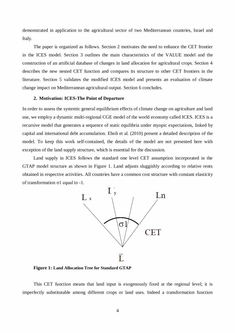
similar fashion. For example, the production of plant based fibers rises until year 2020 by more than

5% following the impact of climate change and then falls by about 18% by 2050. Outputs of other

crops are almost unaffected by climate change until year 2020 and decline afterwards.

Figure 8: Climate Change Impact on Agricultural Output in France

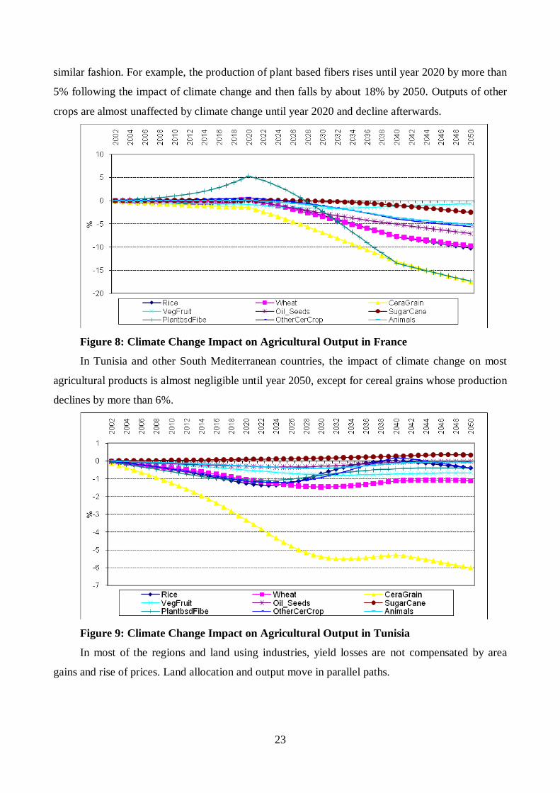
In Tunisia and other South Mediterranean countries, the impact of climate change on most

agricultural products is almost negligible until year 2050, except for cereal grains whose production

declines by more than 6%.

Figure 9: Climate Change Impact on Agricultural Output in Tunisia

In most of the regions and land using industries, yield losses are not compensated by area

gains and rise of prices. Land allocation and output move in parallel paths.

24

At the world level, climate change until year 2050 mostly hits world output of cereal grain

(Figure 10). The relatively high yield loss is followed by general reduction in land allocation for

this crop reducing total output. Other crop products are either unaffected or even increase.

Figure 10: Climate Change Impact on World Agricultural Output

6. Conclusions

This study presents an internal modification of a CGE model employing inputs from a partial

equilibrium model for the agricultural sector, with the aim of making the model more suitable to

quantify and analyze the long-term socio-economic and environmental consequences of different

climate scenarios on agriculture. The methodology is innovative as it combines state-of-the-art

knowledge from economic and biophysical sources. Initially, to this end, the VALUE model is

applied to two Mediterrenean countries: Israel and Italy. The information from the VALUE model

was incorporated in the economic model ICES to improve the agricultural production structure. The

new land allocation method that was introduced takes into account the variation of substitutability

between different types of land and water uses. It captures agronomic features included in the

VALUE model. This modification gives a better representation of heterogeneous information of

land productivity to the economic framework. Climate impacts and policy evaluation with

ICESValue become reinforced due to the more refined system of land allocation. Our results reflect

the significance of structural features specific to agriculture for consistent analyses of climate

change impacts on land use, future crop patterns and economic development.

The main contribution of this paper is in highlighting the need for more detailed land market

in modelling crop supply response. The modifications introduced in the model address frequently

voiced criticisms that CGE models have a limited ability to capture crop specific supply response in

25

agriculture. The originality of this exercise lies in the use of empirically estimated parameters,

which in other similar studies are generally assumed or guessed. Notably, we suggest diverse land

CET frontiers to two main ecological regions in the Mediterranean basin, for more accurate

representation of agronomic characteristics.

References

Angelakis, A.N. and B. Durham. 2008. ―Water recycling and reuse in EUREAU countries: Trends

and challenges.‖ Desalination 218: pp. 3-12.

Atwood, J.A. and G.A. Helmers. 1998. ―Examining Quantity and Quality Effects of Restricting

Nitrogen Applications to Feedgrains‖ in American Journal of Agricultural Economics, N°80,

pp. 369-81.

Bindi, M. and M. Moriondo. 2005. ―Impact of a 2 °C global temperature rise on the Mediterranean

region: Agriculture analysis assessment‖, in Climate change impacts in the Mediterranean

resulting from a 2 °C global temperature rise, Giannakopoulos, C., Bindi, M., Moriondo, M.,

and T. Tin, (Eds.), WWF , 54–66.

Birur, D., T.W. Hertel, and W. Tyner. 2008. ―Impact of Biofuel Production on World Agricultural

Markets: A Computable General Equilibrium Analysis‖, GTAP Working Paper No 53,

Center for Global Trade Analysis, Purdue University.

Choi S. 2004. "The Potential and Cost of Carbon Sequestration in Agricultural Soil: An Empirical

Study with a Dynamic Model fo the Midwestern U.S." Ph.D. Thesis, Department of

Agricultural, Environmental, and Development Economics, Ohio State University.

Eboli F., R. Parrado and R. Roson. 2010. ―Climate Change Feedback on Economic Growth:

Explorations with a Dynamic General Equilibrium Model‖, Environment and Development

Economics, Volume 15, Issue 05 , pp 515 -533

Halperin comittee report, 1999. "Principles of Permitting Irrigation with Wastewater," Online

August 2007 (Hebrew):

http://www.health.gov.il/pages/default.asp?maincat=26&catId=104&PageId=799

Hertel T.W., S. Rose, R.S.J. Tol. 2009. ―Land Use in Computable General Equilibrium Models: An

Overview‖. In: Hertel TW, Rose S, Tol R S J Economic Analysis of Land Use in Global

Climate Change Policy, Abingdon: Routledge

Howitt, R.E. 1995. "Positive Mathematical Programming," American Journal of Agricultural

Economics 77(2): 329-342.

Huang, H., F. van Tongeren, J. Dewbre, and H. van Meijl. 2004. ―A New Representation of

Agricultural Production Technology in GTAP‖ Paper Presented at the 7th Annual Conference

26

on Global Economic Analysis, Washington DC, USA.

https://www.gtap.agecon.purdue.edu/resources/res_display.asp?RecordID=1504

ICBS—Israel Central Bureau of Statistics. 2004. Online, http://www1.cbs.gov.il/reader, August

2008 (Hebrew).

IDDRI. 2009. The Future of the Mediterranean: from impacts of climate change to adaptation issues

IMAGE. 2001. The IMAGE 2.2 Implementation of the SRES Scenarios, RIVM CD-ROM

Publication 481508018. Bilthoven. The Netherlands.

INCCC. 2010. Israel National Report on Climate Change - Second National Communication to the

Conference of the Parties to the United Nations Framework Convention on Climate Change.

State of Israel Ministry of the Environment.

http://www.sviva.gov.il/Enviroment/Static/Binaries/index_pirsumim/p0578-english_1.pdf Accessed

December 2010.

ISTAT. Online. http://agri.istat.it/, accessed November 2010.

Kan, I. 2003. "Effects of drainage-salinity evolution on irrigation management." Water Resources

Research, 39(12):pp. 1377-1388.

Kan, I. 2008. ―Yield Quality and Irrigation with Saline Water Under Environmental Limitations:

The Case of Processing Tomatoes in California.‖ Agricultural Economics 38: 57-66.

Kan, I., K.A., Schwabe and K.C. Knapp. 2002. ―Microeconomics of Irrigation with Saline Water,‖

Journal of Agricultural and Resource Economics 27(1):16-39.

Keeney, R., and T.W. Hertel. 2009. ―The Indirect Land Use Impacts of U.S. Biofuel Policies: The

Importance of Acreage, Yield, and Bilateral Trade Responses‖ American Journal of

Agricultural Economics 91(4): 895 – 909.

Krichak, S.O., P. Alpert, and P. Kunin. 2010. Numerical simulation of seasonal distribution of

precipitation over the eastern Mediterranean with a RCM, Climate Dynamics 34:47–59.

Knapp, K. C. 1992. ―Irrigation Management and Investment Under Saline, Limited Drainage

Conditions. 1. Model Formulation.‖ Water Resources Research 28(12):3085-3090.

Lee, H.-L., T. W. Hertel, B. Sohngen, N. Ramankutty and U.S. Environmental Protection Agency.

2005. GTAP Greenhouse Gases Emissions Data Base. Center for Global Trade Analysis,

Purdue University, West Lafayette, IN47907, U.S.A.

Lee, H-L., T.W. Hertel, and S. Rose, and M. Avetisyan. 2008. ―An Integrated Global Land Use

Data Base for CGE Analysis of Climate Policy Options‖ Center for Global Trade Analysis,

Purdue University Purdue University GTAP Working Paper 42.

Letey, J., and A. Dinar. 1986. ―Simulated Crop-Water Production Functions for Several Crops

When Irrigated With Saline Waters.‖ Hilgardia 54(1):pp. 1-32.

27

Lubowski R., A. Plantinga and R. Stavins. 2005. Land-Use Change and Carbon Sinks: Econometric

Estimation of the Carbon Sequestration Supply Function. Regulatory Policy Program

Working Paper RPP-2005-01. Cambridge, MA: Center for Business and Government, John

F. Kennedy School of Government, Harvard University.

Maas, E. V., and G. J. Hoffman. 1977. Crop Salt Tolerance - Current Assessment. Journal of the

Irrigation and Drainage Division. American Society of Civil Engineers 103:115-134.

Ministry of Agriculture and Rural Development. 2000. Sample Cost Studies for Growing

Plantations. (Hebrew).

Ministry of Agriculture and Rural Development. 2003. Sample Cost Studies for Growing Field

Crops and Vegetables. (Hebrew).

National Institute of Agricultural Economics. Online, http://www1.inea.it/rica/index.html. Accessed

November 2010.

Okagawa, A. and K. BAN. 2008. Estimation of substitution elasticities for CGE models. Discussion

Papers in Economics and Business, No 08-16, Osaka University, Graduate School of

Economics and Osaka School of International Public Policy (OSIPP),

http://econpapers.repec.org/RePEc:osk:wpaper:0816 .

Palatnik R. R. and R. Roson. (2009) ―Climate Change Assessment and Agriculture in General

Equilibrium Models: Alternative Modeling Strategies‖. Working Papers Department of

Economics Ca’ Foscari University of Venice No. 08/WP/2009 ISSN 1827-3580 Available at:

http://www.dse.unive.it/fileadmin/templates/dse/wp/WP_2009/WP_DSE_palatnik_roson_08

_09.pdf

Parry, M.L., O.F. Canziani, J.P. Palutikof and Co-authors. 2007. Technical Summary. Climate

Change 2007: Impacts, Adaptation and Vulnerability. Contribution of Working Group II to

the Fourth Assessment Report of the Intergovernmental Panel on Climate Change, M.L.

Parry, O.F. Canziani, J.P. Palutikof, P.J. van der Linden and C.E. Hanson, Eds., Cambridge

University Press, Cambridge, UK, 23-78.

Plessner, Y., and E. Feinerman. 1995. On the economics of irrigation with saline water: A dynamic

analysis. Natural Resource Modeling 9:255-276.

Röhm, O. and S. Dabbert. 2003. Integrating Agri-Environmental Programs into Regional

Production Models: An Extension of Positive Mathematical Programming. American

Journal of Agricultural Economics 85(1): 254-265.

Schwabe, K.A., I. Kan, and K.C. Knapp 2006. Drainwater Management to Reduce Salinity

Problems in Irrigated Agriculture. American Journal of Agricultural Economics 88(1): 133-

149.

28

Shani, U., A. Ben-Gal, E. Tripler, and L.M. Dudley. 2007. Plant Response to the Soil Environment:

An Analytical Model Integrating Yield, Water, Soil Type and Salinity.‖ Water Resources

Research 43: W08418. doi: 10.1029/2006WR005313.

Shumway, C. R. and A. A. Powell. 1984. A Critique of the Constant Elasticity of Transformation (CET)

Linear Supply System. Western Journal of Agricultural Economics 9(2):314-321.

Timilsina, G.R., J.C. Beghin, D. van der Mensbrugghe and S. Mevel. 2010. The Impacts of Biofuel

Targets on Land-Use Change and Food Supply: a Global CGE Assessment. World Bank

Policy Research Working Paper No. WPS 5513, Dec 2010.

Tol, R.S.J. 2002a. New Estimates of the Damage Costs of Climate Change, Part I: Benchmark

Estimates’, Environmental and Resource Economics, 21(1): 47-73.

Tol, R.S.J. 2002b New Estimates of the Damage Costs of Climate Change, Part II: Dynamic

Estimates’, Environmental and Resource Economics, 21(1):135-160.

Tsimplis M.N., M. Marcos, and S. Somot. 2007. 21st century Mediterranean sea level rise: steric

and atmospheric pressure contributions from a regional model. Global and Planetary Change,

63, p. 105-111.

Villevieille A. (ss dir.) et al., 1997. Les risques naturels en Méditerranée. Situation et perspectives.

Economica, Blue Plan fascicules , n° 10, 157 p.

29

Annex A

Table A1: ICES Sectoral and Regional Disaggregation

Sectors

Land using Industries Additional Industries

Rice Forestry

Wheat Fishing

Cereal Crops Coal

Vegetable Fruits Oil

Oil Seeds Gas

Sugar Cane Oil Products

Plant-Based Fibers Electricity

Other Crops Other industries

Animals Market Services

Non-Market Services

Regions

Code Description

Italy Italy

Spain Spain

France France

Greece Greece

Malta Malta

Cyprus Cyprus

Slovenia Slovenia

Croatia Croatia

FYug Bosnia, Monaco, Serbia*

Albania Albania

Turkey Turkey

Tunisia Tunisia

Morocco Morocco

RoNAfrica Rest of North Africa [Algeria, Egypt, Libya]*

RoMdEast Rest of Middle East [Israel, Lebanon, Palestinian Authority, Syria]*

RoNME non-Mediterranean Europe

RoA1 Other Annex 1 countries

ChInd China & India

ROW Rest of the World

30

Annex B

Table B1. Allocation of 45 groups of crops incorporated by VALUE for Israel into 8 land-

using industries in ICES

ICES category Crop(s)

Wheat Wheat

Vegetables & Fruits

Orange, grapefruit, lemon, apple, pear, peach, plum, grape, banana, olive, almond, avocado, palm, tomato, cucumber, eggplant, pepper, marrow, strawberry, onion, carrot, lettuce, bean,

cabbage, cauliflower, celery, radish, artichoke, garlic, sugar-melon, water-melon, potato

Sugar Cane NA

Rice NA

Plant-Based

Fiber

Cotton

Oil Seeds Sunflower, corn

Cereal Grains Barley, chickpea, pea, groundnut

Forage Summer forage, winter forage

Table B2. Allocation of the 45 groups of crops incorporated by VALUE for Italy into 8 land-

using industries in ICES

Category Code Crop(s)

Wheat WHT Common wheat and spelt, Durum wheat

Vegetables,

fruits and nuts

V_F Potatoes, Fresh vegetables outdoor – open field, Fresh vegetables outdoor –

market gardening, Fresh vegetables under glass, Fresh fruit of temperate climate

zones, Fruit of subtropical climate zones, Nuts, Citrus plantations, Vineyard - quality wine, Vineyard - other wines, Vineyard - table grapes

Plants used for

sugar

manufacturing

C_B Sugar beet

Paddy rice PDR Rice

Plant fibers PFB Flax, Hemp

Oil seeds and oleaginous

fruit

OSD Rape and turnip rape, Sunflower, Soya, Olive plantations - table olives, Olive plantations - olives for oil production

Other grains GRO Rye, Barley, Oats, Grain maize, Other cereals for the production of grain, Protein

crops for the production of grain

Other crops OCR Fodder roots and brassicas, Flowers and ornamental plants outdoor, Flowers and

ornamental plants under glass, Forage plants - temporary grass, Forage plants -

other green fodder, Tobacco