Land Use Change and Agricultural Intensification:

Key Research Questions and Innovative Modeling Approaches

JunJie Wu and Man Li

A Background Paper Submitted to

The International Food Policy Research Institute

Under Agreement # 200002.000.180 515-01-01

Final Report, November 2013

Abstract. This paper reviews land use modeling approaches for assessing the economic and

environmental impacts of agricultural intensification. It discusses the theoretical foundations of

the modeling approaches, describes how to parameterize such models when micro-level data are

available, and examines how to integrate them with biophysical models for policy evaluation.

Based on the literature review, the paper identifies key research questions and discusses

appropriate methods and data and promising research areas for investigating those questions.

2

1. Introduction

Agriculture around the world will face tremendous pressure for intensification over the next 50

years. The United Nations forecasts the world population will increase by one third from 2013–

2050. This will dramatically increase the demand for food. The economic transformation

currently under way in China, India and other developing nations also has profound implications

for global resource demand and environmental conditions. As these countries shift from largely

agrarian to industrial economies, their demand for food, energy and natural resources will

increase with rising income. Agriculture is expected to meet growing demands for food and

fiber. At the same time, agriculture is also expected to provide increased animal welfare and

more ecosystem services and play a major role in producing renewable energy, including

bioenergy. These new demands will intensify competition for land around the world and will put

the role of agricultural intensification at the center stage.

Agricultural intensification is a production system conventionally characterized by a low

fallow ratio and an intensive use of inputs, such as capital, labor, pesticides, and chemical

fertilizers, to raise agricultural yields, thereby increasing farmers’ income and reducing poverty.

It remains a question, however, whether such intensification can harmonize food production and

environmental protection. Previous studies demonstrated that intensive agricultural production

has led to increased erosion, lower soil fertility, and reduced biodiversity (Matson et al. 1997).

Intensification may cause conversions of marginal lands, such as grasslands or rangeland, to crop

production, leading to land degradation (Li et al., 2013). Intensification may also have negative

regional externalities because water use and chemical runoff can impact areas beyond those

actually cultivated (Matson et al. 1997; Tilman et al. 2002).

3

In response to the global pressure for balancing economic development and

environmental protection, the IFPRI-led BioSight project was established. This project aims to

provide a novel and integrated approach to strategic policy analysis for sustainable agricultural

intensification at the intersection of food, water, land, energy, and the environment. Sustainable

agricultural intensification is generally defined as a process whereby agricultural yields are

increased without generating adverse environmental impacts. Sustainable agricultural

intensification includes a range of farming practices, from specific agro-ecological methods, to

practices used in commercial agriculture, to biotechnology. This concept has received increased

attentions in some high-level political and scientific circles in recent years because it offers a

potentially practical pathway towards the goal of producing more food with less impact on

environment. BioSight aims to advance the science of integrated bioeconomic modeling by

developing a set of tools and data with strong micro-level and spatially-explicit grounding to (1)

improve calibration of existing models, (2) extend their analysis to address alternative policies

for scaling up of sustainable intensification, and (3) generate actionable policy recommendations

on sustainable intensification that are appropriate to short- and medium-term outlooks.

To support BioSight’s development of models, tools, and problem-focused analytics, this

report reviews land-use modeling approaches for assessing the environmental and ecological

impacts of agricultural intensification. The goal of this paper is to lay a solid foundation for the

development of models, tools, and problem-focused analytics that explore the impacts and

implications of agricultural intensification. The specific objectives are:

1. Conduct a thorough literature review on land use modeling approaches for assessing the

economic and environmental impacts of agricultural intensification, and describe how best to

parameterize such models, especially those dealing with the data-rich environment, e.g.,

4

when micro-level household surveys are available, or when detailed spatial data of land use

and land cover exist.

2. Review the methods for integrating land use models and biophysical models to assess the

impact of land use change on ecosystem services, and based on the literature review, and

identify important methodological/data gaps in the literature.

3. Identify 3–5 top research questions relating to land use change and sustainable intensification

that have important policy implications and scientific significance, and discuss the

appropriate methods and data for investigating these research questions.

4. Propose a set of promising study areas in which these questions could be explored and

provide guidance as to the minimum data requirements.

In this paper, land use change refers to more than simply the pattern of different land

covers (e.g., cropland, grassland, rangeland) in space. Rather, it includes any changes in

arrangements, activities, and inputs that people undertake in a certain land cover type. In this

sense, agricultural intensification is a major cause of land use change. Agricultural

intensification can occur at both the intensive margin and the extensive margin. Agricultural

intensification occurs at the intensive margin when more input is used for a given land area (e.g.,

more fertilizer application per acre in the production of corn). Agricultural intensification occurs

at the extensive margin when a less input-intensive land use is converted to a more input-

intensive land use (e.g., conversions of grassland to crop production).

Section 2 discusses the theoretical foundations of the modeling approaches and describes

how to parameterize such models when aggregate or micro-level data are available. Section 3

discusses the environmental/ecological impacts of agricultural intensification and land use

change and examines how to integrate economic and biophysical models to assess the impacts.

5

Based on the literature review, section 4 identifies important research questions that have

important policy implications and scientific significance, and reviews the appropriate

methodology and data for investigating these research questions. Section 5 concludes with a brief

discussion of promising study areas.

2. Theories and Econometric Approaches for Modeling Land Use

Economic studies of land use and land use change can be arrayed in a number of dimensions:

theoretical versus empirical; structural versus reduced form; econometric versus other empirical

approaches; farm, regional, national, versus international-level studies; disaggregate versus

aggregate; extensive-margin versus intensive-margin studies; drivers versus consequences-

orientated studies, policy versus methods-orientated studies (see Table 1). The first three

dimensions are related to the study method, the next three to the study scope, and the last two to

the study objective. For example, Irwin and Wrenn (forthcoming) provide an overview and

assessment of the main methods used to model land use change and classify land use models

along two dimensions: first, models that are structural versus reduced form and second,

econometric models versus other empirical approaches that are used to specify parameter values.

Duke and Wu (forthcoming) arrange the chapters in the Oxford Handbook of Land Economics in

several dimensions. They divide the chapters into four main sections focusing on drivers of land

use change, consequences of land use change, methodological developments, and the economics

of land use law and policy, respectively. The methodological section includes chapters that

focus on econometric, simulation, and experimental methods, respectively.

6

Table 1. Dimensions for Arraying Land-Use Studies

Dimensions Examples

Theoretical vs. empirical Capozza and Helsley (1989) vs.

Li et al. (2013)

Structural vs. reduced form Walsh, R. (2007) vs.

Chavas and Holt (1990)

Econometric vs. other approaches Wu and Cho (2003) vs.

Parker et al (2003)

Disaggregate vs. aggregate Wu et al (2004) vs.

Chavas and Holt (1990)

Parcel, farm, regional, national, vs. international Li et al (2013) vs. Wu and Adams

(2002) vs. Chavas and Holt (1990)

Extensive- vs. intensive-margin studies Wu (1999) vs. Babcock and

Hennessy (1996)

Drivers vs. consequences of land use change Li et al (2013) vs.

Wu and Babcock (1999).

Policy vs. theoretical/method-oriented studies Just and Antle (1990) vs. Wu and

Cho (2007)

To a large extent, the scope and method of empirical studies are driven by the available

data. Applied economists must wrestle with the tradeoff between a theoretically consistent model

specification and tractability constraints imposed by data (Wu and Adams, 2002). With this in

mind and considering the goal of the BioSight project, we discuss the different theories and

empirical approaches for modeling land use when different levels of data are available in this

section.

7

2.1 Modeling land use with micro-level data

When household-level survey data are available, the microparameter distribution model can

serve as a conceptual framework for modeling land allocation decisions (We and Segerson,

1995). Specifically, consider a farm that has Nj acres of land of type j (j = 1 ..., J). Land types can

be distinguished by land characteristics such as soil type, slope and permeability. The total

acreage for the farm is then N = N1 + N2 +…+ Nj. For each land type, the farmer must decide

how to allocate the Nj acres across crops. Let i = 1, ..., I index crops and let m = 1 ..., M index

variable inputs (including pesticides and fertilizers). The farmer faces exogenous crop prices p =

(pi, ..., pI) and exogenous input prices w = (w1, ...., wM), and chooses the amount of land type j to

produce crop i, nij. Let p ij(pi, w, nij) denote the restricted profit function for crop i grown on land

type j, given nij. For each land type, the farmer then chooses the land allocation that maximizes

total profit:

(1) Max(n1 j ,...,nIj )

p ij pi , w, nij( )i=1

I

å

subject to

(2) N1j + N2j +…+ NIj = Nj.

The solution to this problem gives the optimal land allocation for type j land:

nij

* = nij p, w, N j( ) . Assume this function is homogeneous of degree 1 in Nj. Then

nij

* = nij p, w, 1( )N j. The total acreage devoted to production of crop i is then given by:

(3) ni

* = nij

* pi , w, 1( )N j

j=1

J

å .

Equation (3) can be written in share form as

8

(4) si

* =ni

*

N = nij

* pi , w, 1( )N j

N

æ

èçö

ø÷j=1

J

å º sij

* p, w, N1

N,...,

NJ

N

æ

èçö

ø÷

Note that the shares depend on all output and input prices, and on the entire distribution of land

characteristics for the farm.

There are two approaches to the estimation of the share equations in equation (4) (Wu

and Segerson, 1995). The first is to specify a flexible functional form, such as translog or

normalized quadratic, for the restricted profit function and then derive the implied functional

form for the share equations. This is the approach taken by Moore and Negri (1992) as well as by

others who have studied multi-product acreage or supply decisions (e.g., Weaver, 1983;

Shumway, 1983). Alternatively, one can assume a flexible functional form for the share

equations themselves. For example, the share equations can be assumed to take the logistic

form, as in Considine and Mount; Chavas and Segerson (1986); Wu and Segerson (1995), Wu

and Tanaka (2005). The first approach has the advantage of providing a theoretical link between

the forms of the profit function and the share equations. However, the desirable local properties

do not necessarily hold globally (Wales, 1977). In addition, it does not ensure that predicted

shares lie in the zero-one interval. In contrast, use of the logistic form ensures that the shares will

lie between zero and one. The logit model has also been shown to outperform other flexible

functional forms, such as the Almost Ideal Demand System and the translog (Lutton and

LeBlanc, 1984; Rothman, Hong, and Mount, 1993) and has been widely used in economic

analysis, including the study of farmers’ land allocation decisions (Lichtenberg, 1989; Wu and

Segerson, 1995; Hardie and Parks, 1997; Plantinga, Mauldin, and Miller, 1999), the choice of

irrigation technologies (Caswell and Zilberman, 1985), and the choice of alternative crop

management practices (Wu and Babcock, 1998).

9

Micro-level data may also exist for a selected sample of individual parcels. For example,

the U.S. Natural Resource Inventory (NRI) is conducted every five years to determine the status,

condition, and trend in the nation’s soil, water, and other related resources. It contains land use

and conservation practices information at more than 800,000 sites (fields) across the continental

United States. In this case, the random utility model can serve as a theoretical foundation for

modeling land use choices at individual parcels. Specifically, let u

ij( X

ij) be the farmer’s utility

from growing crop i on parcel j. Because the farmer’s preferences are unknown to the researcher,

u

ij( X

ij) can be considered a random variable and be written as

(5) u

ij(X

ij) = v

ij(X

ij) + e

ij, i = 1, 2, …, N, j=o,c.

where v

ij( X

ij) is the mean of

u

ij( X

ij) and is specified as

v

ij( X

ij) = ¢X

ijb

i, and ij is a random

error term. If the residuals ij are assumed to be independently and identically distributed with

the extreme value distribution, then the probability that the farmer will choose crop i on parcel j

is given by a multinomial logit model (Maddala, p. 60):

(6)

Pij

=e

¢Xijb

i

e¢Xkjb

k

i=1

I

å, i = 1,..., I .

The marginal effects of chances in explanatory variables on crop choices in a logit model

are nonlinear combinations of the explanatory variables and can be written as

(7) ¶Pij

¶ Xij

= Pij bi - Pkjbkj

k=1

I

åæ

èçö

ø÷.

The sign and magnitude of this marginal effect have no direct relationship with any specific

coefficient.

10

2.2 Modeling land use with aggregate data

When micro-level data are unavailable, relationships representing the behavior of individual

economic agents are frequently estimated using aggregate or “macro” data (Grunfeld and

Griliches, 1960). These empirical macro relationships are then used for making inferences about

individual behavior and/or for making aggregate predictions. Two potential problems may arise

from this practice (Wu and Adams, 2002). One, which is often referred to as the aggregation

problem, concerns the connections between micro and macro behavior (Chambers and Pope,

1991). If aggregate relationships are used to make inferences about individual behavior, one

must consider the conditions under which the distribution of individual characteristics can be

ignored so that the results can be treated as if they are the outcome of the decision of a single

“representative” firm or consumer. If these conditions are met, the relationships derived from

micro theory can be estimated with aggregate data and behavioral interpretations can be made

from the estimated parameters.

The second problem concerns the relative accuracy of predictions made by micro and

macro models. With the advance of data collection and management technologies such as

Geographic Information Systems (GIS) and satellite images, more and more micro-level,

spatially articulated data are becoming available. With these data, it is increasingly possible to

estimate micro models and then statistically aggregate the micro-level predictions to the

aggregate level by using the distribution of individual characteristics. The question is whether

the micro approach, facilitated by the availability of micro data, will provide better predictions of

aggregate outcomes than traditional aggregate models.

A large body of literature has focused on the aggregation problem in general and two

lines of inquiry in particular (Wu and Adams, 2002). The first seeks the requisite conditions on

11

micro behavior for a representative producer or consumer to exist (Gorman (1953); Muellbauer

(1975); Klein (1946); Theil (1971); Hildenbrand (1983); Chiappori (1985); Stoker (1984);

Blackorby and Schworm (1988)). These conditions are often found to be quite stringent. The

second line of inquiry has focused on the problem of ‘aggregation bias,’ defined by the

derivation of the macro parameters from the average of the corresponding micro parameters

(e.g., Theil, 1971; Gupta, 1971; Sasaki, 1978; Lee et al., 1989; Shumway, 1995; Love, 1999).

In contrast to the aggregation problem, the issue of prediction accuracy has received less

attention. In a seminal paper, Grunfeld and Griliches (GG) (1960) examined the relative power

of micro and macro models for explaining the variability of the aggregate dependent variable and

found that the aggregate equation may explain the aggregate data better than a combination of

micro equations. Sasaki (1978) reexamined the issue using data from four Japanese industries

and found that the explanatory power of the macro models is not necessarily higher than that of

micro models. Pesaran et al. (1989) developed a more general criterion for choosing between

micro and macro models and applied it to labor demand in UK industries. They found that for

the manufacturing industries the prediction criterion marginally favors the aggregate model but

over all industries the disaggregate models are strongly preferred. Wu and Adams (2002)

examined the issue in the context of predicting land allocation. They show that even in the

context of linear prediction models the issue of whether one should choose micro or macro

models to make aggregate predictions cannot be generally resolved by a priori reasoning.

Because of a lack of disaggregate data, most acreage response models are estimated using

regional or national data (e.g., Houck and Ryan, 1972; Lidman and Bawden, 1974; Chavas and

Holt, 1990; Chavas, Pope, and Kao, 1983). For example, Lichtenberg (1989) estimated a county-

level acreage response model to examine the interaction between land quality, cropping patterns,

12

and irrigation development. Wu and Segerson (1995) estimated a similar model to examine the

effect of government commodity programs and land characteristics on groundwater pollution in

Wisconsin. Hardie and Parks (1997) used county level data to analyze the impact of land quality

on land allocation between agriculture and forests. In these county-level analyses, Pijt is

estimated as the share of potential cropland allocated to crop i in county j in year t, and the beta

parameters are estimated using the following logistic regression equations, which are derived by

taking the log of the ratio of Pijt and PIjt in (6):

(8) lnPijt

PIjt

æ

èç

ö

ø÷ = ¢Xijt i

b +vijt, i = 1, …, (I-1)

where b I is normalized to zero to reduce the indeterminacy in the model (Greene, 1990, p. 697).

Because county size, cultivation history, and other disturbance factors differ across

counties, heteroskedasticity may exist in the county-level model. Heteroskedasticity can be

tested using the Lagrange multiplier test (Greene, 1990, 1990, p. 467). Also, because the

disturbances affecting one crop in one year may affect the same crop in other years,

autocorrelation was tested using the Durbin test. In addition, with land allocation imposing joint

production decisions and disturbances for different crops reflecting common factors (e.g.,

climate and the general state of the economy), contemporaneous correlation (i.e., correlation

between error terms for different crops) may be present. Wu and Brorsen (1995) discuss tests for

detecting these econometric problems and propose an empirical procedure that can be used to

address all of these econometric problems at the same time. Finally, because the disturbances

affecting one county may also affect the neighboring counties, spatial autocorrelations may exist.

13

It is very challenging to correct the spatial autocorrelation in the logistic model. Li et al. (2013)

proposes an approach to address this problem in a recent study.

3. Modeling the Environmental/Ecological Impacts of Land Use

So far we have focused on the theory and methods for analyzing the drivers of land use change.

But land use change can have wide-ranging environmental/ecological consequences. When

wetlands are drained for crop production, it will affect the probability of flooding lower in the

watershed, the flow of nutrients through ecosystems and water quality in adjoining areas. When

natural habitats are modified to serve human uses, valuable ecosystem services may be altered or

destroyed. With the increase in human population and scope of economic activity, there are

growing concerns about the impact of human actions on natural systems.

Natural systems provide a broad range of ecosystem services upon which humans and all

other species depend. The list of important ecosystem services includes: water purification; flood

control and soil retention; nutrient cycling; generation and renewal of soil and soil productivity;

crop pollination; pest control; maintenance of species and genetic information; composition of

the atmosphere and climate stabilization. Land use change not only affects the provision of these

vital ecosystem services, but is also affected by them. Although it may be true that individual

land management decisions do not threaten the life support in total, their cumulative impact may

cause important local changes to ecosystems and contribute to changes in larger-scale processes

such as global climate change. Figure 1 below illustrates the interactions between human and

ecological systems through land use change. Table A1 in the Appendix provides a

comprehensive list of references on the effect of land use and land use change on selected

watershed health indicators

14

Figure 1. Interactions between human and ecosystem through land use change

In this section, we first review and assess the economic literature that examines how land change

affects provision of several specific ecosystem services. We then discuss how economic and

biophysical models could be integrated for policy analysis evaluation.

3.1 Land use and water quality and quantity

It is now well established that economic activities can cause water pollution and that agricultural

land uses in particular are a source of many contaminants. The environmental impacts of land

use change depends on land characteristics, such as soil type, depth to groundwater, and the

Source: Modified based on McDonnell, et al. (2010)

15

underlying geological structure of the land. Since land uses respond to government policies,

those policies can also play an important role in determining the level of water quality.

Much research has focused on the effect of land use on water quality. These studies can

be categorized based on the types of land use they analyze. For example, there is a large body of

literature on the effect of agricultural land use (cropping patterns and farming practices) on water

quality. There are also studies that focus on the effect of forestland or wetland on water quality

or compare their effects with agricultural and other land uses. Studies in each category can be

further divided into subcategories. For example, studies on the effect of agricultural land use on

water quality can be further divided into subcategories in two different ways. One way is based

on the level of model aggregation and the size of study region. For example, there are a great

number of studies that examine the effect of agricultural land use and practices on water quality

at the field or watershed level. There are also studies that examine the issue at the regional or

national level. An alternative way to categorize the studies is based on the various linkages they

model. For example, many studies have modeled the effect of cropping patterns and farming

practices on water quality, without examining how the decisions that led to that cropping patterns

and farming practices were made. Other studies have systematically modeled the process from

land use decisions to water quality.

It has long been recognized that agricultural land use and practices can cause water

pollution and the effect is influenced by government policies (Just and Bockstael 1991; Wu and

Segerson 1995). A major challenge to evaluating the effect is to account for the spatial

heterogeneity of land quality and other physical characteristics. Land uses and farming practices

vary from farm to farm, and affect water quality. In addition, because physical attributes of land

are not homogeneous, water pollution can vary dramatically across farms that have the same land

16

use and farming practices. Climate also plays a role in determining the effect of land use and

farming practices on water quality. Thus, it is necessary to identify the joint distribution of

farming practices, land characteristics, and weather in order to determine the effect of land use

and farming practices on water quality. Because spatial heterogeneity adds a spatial dimension

to the analysis, it complicates the design of models intended to capture the impacts of land use on

water quality.

A number of studies have examined the impact of agricultural land use and practices on

water quality at the field, farm, or watershed levels (e.g., DeRoo, 1980; Hallberg 1989; Gilliam

and Hoyt 1987; Tillman et al. 2002). These studies have linked water pollution to land use,

fertilizer and chemical application rates, crop management practices, and topographic and

hydrological characteristics. For example, in DeRoo (1980), nitrate concentrations in wells

around and in shade tobacco tents and turf plots on two Connecticut farms were monitored. At

one farm, less fertilizer was used. Nitrate concentrations averaged 2.5 mg/L in groundwater

entering the farm and 4 mg/L leaving. After rainfall, concentrations in the downstream wells

were found to be over 10 mg/L. At the other farm, intensive fertilizer application resulted in

average year round nitrate concentration of 20 mg/L. DeRoo (1980) concluded that over-

fertilization on easily leachable soils led to high nitrate concentration in well water downstream

from the crop land. Gilliam and Hoyt (1987) examined nitrogen movement under different

management practices. After an extensive literature review, Gilliam and Hoyt (1987) concluded

that under no-till practices the amount of nitrogen in soil is higher than under conventional

tillage practices. Thus, the use of no-till practices instead of conventional tillage increases the

possibility of leaching. Conservation tillage practices, however, reduce nitrogen loss from

surface run-off. The increased nitrogen in the soil makes more nitrogen available to leach to

17

groundwater. Anderson et al. (1985) examined the relationship between pesticide application

rates and groundwater contamination of wells in Washington County, Rhode Island. Using data

for individual wells, they regressed observed levels of contamination of the pesticide TEMIK

(Aldicarb) on previous application rates and well characteristics. The well characteristics

considered include depth to water and the distance of the well from the point of

application. They found that contamination levels were significantly affected by application

rates, with the effect decaying with both the well depth and the distance from the field.

The increased concern over water quality raises the issue about the scope and trend of

water pollution from agriculture. To address the issue, several national inventories have been

conducted in the United States to determine the status and trend of groundwater or surface

pollution. These inventories have provided data for several summaries of water-quality

conditions in the nation (e.g., Mueller et al. 1995; Omernik 1977). Smith and his associates

(Smith et al. 1987) have assessed water quality trends in major U.S. rivers using water quality

monitoring data. However, as Smith at al. (1987) point out, because the sampled pollutant

concentrations come from both agricultural and non-agricultural sources, the extent to which

changes in agricultural practices are reflected in the trends is largely a matter of conjecture. In

addition, substantial variations in climate confounded assessment of water quality improvements

that might have occurred because of changes in management practices. The groundwater quality

monitoring in the Big Spring Basin in Iowa shows that, because nitrates tend to accumulate in

the soil-water systems during a dry year and to be mobilized by the excessive precipitation and

recharge in a wet year, changes in mean annual nitrate concentration parallel changes in

groundwater discharge rather than changes in agricultural management practices (Rowden et al.

1995). However, this does not necessarily mean that agricultural land use and practices does not

18

cause water quality problems. Mueller et al. (1995) found that nitrate concentrations in 21% of

samples collected beneath agricultural land exceeded the 10 mg/l maximum contamination level

set by the U.S. Environmental Protection Agency. Nitrate-N is the most commonly detected

agricultural chemical in groundwater.

The increased concerns over agricultural water pollution have also fueled the need for

timely information on the location of areas with high potential for water contamination from

agricultural chemical use. Several studies (Nielsen and Lee, 1987; Kellogg, Maizel and Goss,

1992; Wu et al., 1997; Wu et al. 1999) have attempted to provide this information by conducting

national or regional assessment of water contamination potential from agricultural chemical

use. Nielsen and Lee (1987) evaluated groundwater contamination potential from agricultural

chemical use by synthesizing the USGS well-water test data, hydrological information and

nitrogen use data. They found that the drinking water of an estimated 50 million people in the

U.S. came from groundwater that was potentially contaminated from agricultural chemicals and

that potential contamination follows regional trends, suggesting a need for targeting

strategies. This study, however, did not incorporate production system information into the

assessment.

Kellogg, Maizel and Goss (1992) developed a groundwater vulnerability index for

nitrogen fertilizer to identify high-risk areas in the United States and updated their results in

1994 to incorporate revised estimates of precipitation and the 1992 National Resources Inventory

data. They found that total number of high risk areas of pesticide leaching were 156.5 million

acres in 1982 and 140.5 million acres in 1992. The chemical use was assumed to be the same for

both years. Thus, the reduction in the high risk area of pesticide leaching was a result of changes

in land use alone. Approximately one-half of this reduction was due to the enrollment of

19

cropland in the Conservation Reserve Program. One limitation of their index is that it does not

incorporate crop management practice information (e.g., tillage and conservation practices),

although it synthesizes physical data with land use data. Huang et al. (1992) estimated the

distribution of cropland potentially vulnerable to nitrate-N leaching and found that the Corn Belt

states have most of this cropland.

Wu et al. (1997) assessed potential water pollution from nitrogen use in the U.S. High

Plains by synthesizing physical data with production system information, but used only a few

representative soils to account for soil heterogeneity. They found that counties with great

nitrogen losses tend to be those that are heavily furrow irrigated and/or have large acreage of

corn. Their results suggest that targeting particular soils or production systems may be an

effective strategy for protecting water quality, and that adopting modern irrigation technologies

in heavily irrigated areas may be a key to reducing nitrogen water pollution.

Wu and Babcock (1999) developed a model to identify the spatial patterns of potential

nitrate-N water pollution in the central U.S. and to estimate the effect of alternative farming

practices on potential nitrate water pollution in the region. The model consists of a set of

metamodels that summarize the impacts of soils, climate, crops, and management practices on

potential nitrogen runoff and leaching. The potential for nitrogen runoff and leaching was

estimated for a total of 128,591 sites using information on soil, climate, crop, rotation, tillage,

irrigation, and conservation practices at each site. Thus, this assessment incorporates more

detailed information on production systems and physical characteristics than previous

assessments. For the 12 states in the Central U.S., the average annual N runoff and leaching,

respectively, were estimated to be 5 kg ha and 3 kg ha , which accounted for about 7% and 4%

of total nitrogen applied. The potential for -N runoff was relatively high in much of the Corn

20

Belt, Kansas, and the Nebraska Platte River Basin, and the potential for -N leaching was

relatively high in Ohio, Indiana, and southern Illinois and Missouri. However, because much of

the area with high leaching potential was tile drained, it is likely that a large portion of the

leached N is discharged to surface water, rather than continue downward to groundwater.

3.2 Land use and biodiversity conservation

There is concern that we are in the midst of a human caused extinction crisis that has increased

the current species extinction rates several orders of magnitude above the “natural” or

background rate of extinction (Pimm et al. 1995). The destruction, fragmentation, and alteration

of habitat for human land use are the leading causes of biodiversity decline (Soulé). Czech,

Krausman, and Devers (2000) find that urbanization endangers more species in the mainland

United States than any other human activity. Urbanization leads to an increase in human density

in urban areas, and an associated increase in the concentration of buildings, roads, and fences.

The resulting disturbances (noise, human presence, exotic species, habitat fragmentation,

predation by pets) disrupt wildlife interactions and change wildlife populations and communities

(Knight, Wallace, and Riebsame). Urbanization can also have a significant effect on species

associated with remnants of habitat that are not directly altered, but are surrounded by

development (Rottenborn). As a result, the species richness (the number of species) of many taxa

is often found to decline along the urban-rural gradient, with the lowest richness found in the

urban core.

There is a growing body of literature that examines the effect of land-use changes, in

particular urbanization, on biodiversity (see McKinney (2002) for a review of this literature). For

example, Friesen, Eagles, and Mackay (1995) and Rottenborn (1999) examine the effects of

urbanization on bird communities. White et al. (1997) develop an approach to predict the

21

potential effects of landscape change on different biodiversity measures for terrestrial

vertebrates. Montgomery et al. (1999) build on this approach to search for efficient land use

allocations by estimating the marginal cost of increasing expected biodiversity.

3.3 Land use and carbon sequestration

Land use change such as agricultural intensification plays a significant role in the global carbon

cycle, with two-way interactions. Any climate change from build-up of atmospheric greenhouse

gases can affect land productivity and the allocation of land among major uses. In the other

direction of interaction or feedback, increasing carbon sequestration in agricultural and other

rural land uses is a potentially useful mechanism in global efforts to offset expanding greenhouse

gas emissions. In many studies (e.g., Sedjo et al. 1993, 1995), changes in land uses (e.g.,

afforestation of agricultural land) are examined as the primary vehicle for expanding carbon flux.

A wide range of studies has examined how changes in land uses and land covers may

affect the sequestration of atmospheric carbon by forests and other rural land uses, and how

markets may affect the adjustment and adaptation of rural land uses to climate and ecological

change (Sohngen 2007; Sohngen and Sedjo 2000, 2006; Sohngen and Alig 2000). Evidence from

large-scale ecological models linked to atmospheric models suggests that the role of forests in

the carbon cycle may become more important in the future (Neilson and Marks, 1994). For

instance, forests may provide a positive or negative feedback to the carbon cycle, depending on

the influence of the underlying climate change. Humans may attempt to mitigate the impacts of

climate change by increasing the storage of carbon in forests through tree planting or altered

agricultural practices. Although adaptation in land management is one important factor for

gauging carbon flux feedbacks within the climate system, adaptation in product management can

have important implications for how such adjustments manifest.

22

Most of the economic studies of carbon sink management evaluate policies that

encourage the conversion of agricultural land to forests (e.g., Moulton and Richards 1990;

Adams et al. 1993; Adams et al. 1999; Plantinga, Mauldin, and Miller 1999; Lubowski,

Plantinga, and Stavins 2006; Parks and Hardie 1995). In these studies, the cost of the policy

equals the opportunity costs of agricultural production and benefits are measured as physical

quantities of carbon removed from the atmosphere. A consistent finding is that the costs of

carbon sequestration through afforestation are comparable to, and in some cases lower than, the

costs of alternative approaches such as fuel substitution and improved energy efficiency

(Plantinga, Mauldin and Miller 1999; Stavins 1999; Lubowski, Plantinga, and Stavins 2006).

However, only a few studies have investigated the additional environmental impacts of carbon

sink management such as modification of wildlife habitat or reduction in run-off and leaching of

agricultural chemicals (Plantinga and Wu 2003). If the additional environmental benefits or

costs (“co-benefits”) of carbon sink management are found to be substantial, industrialized

countries may want to adjust the mix of domestic mitigation and abatement strategies used to

meet emissions reduction targets. In addition to carbon sequestration in forests, increasing the

storage of soil carbon through agricultural management (e.g., conservation tillage) has also

received attention in the literature because of its economic potential to improve soil fertility

(Antle et al. 2003; Antle et al. 2007). Richards and Stokes (2004) reviewed studies on forest

carbon sequestration cost and find that afforestation in the United States would sequester 250 to

500 million MgC annually at a price ranging 10–150 USD/MgC. By comparison, Antle et al.

2003), Capalbo et al. (2004), and Pautsch et al. (2001) suggest that conservation tillage can

generate 0.25 to 6.2 million MgC in soil per year at the cost of 12–270 USD/MgC.

23

3.4 Integrate economic and biophysical models for policy analysis

Most of the studies discussed above focus on the effect of land use change and farming practices

on environmental quality and ecosystems, without examining how the decisions that led to the

land use change were made. These studies do not attempt to model land use decisions, but rather

take these decisions as given and simply analyze their impact on water quality and other

ecosystem services. To model the interaction between economic and ecological systems

systematically, we must integrate economic and biophysical models to examines how economic

and policy variables affect land use and how changes in land use in turn affect ecosystems.

A number of studies have systematically modeled the process from land use decisions to

environmental impacts. These studies can be categorized into conceptual and empirical (or

simulation) studies. The conceptual dimensions of land use and water quality have been

explored in several studies, including Hochman and Zilberman (1978), Sharp and Bromley

(1979), Shortle and Dunn (1986), Just and Antle (1990), and Opaluch and Segerson

(1991). These studies show that agricultural and resource policies can affect agricultural

production at both the intensive margin (changes in input use and management practices) and the

extensive margin (changes in cropping patterns) and the resulting effects on water quality depend

on physical attributes. These studies, however, do not provide quantitative estimates of the

effects.

The empirical studies that model both land use decisions and their impact on water

quality can also be classified into disaggregate models and aggregate models. The disaggregated

models are generally site-specific and model micro-unit decisions and the water quality effect of

these decisions at the farm or watershed levels (e.g., Jacobs and Casler 1979; Braden et al. 1989;

Johnson et al. 1991; Taylor 1992; Wu et al. 1994; Helfand and House 1995). Because these

24

studies are site-specific, regional and/or national policy impacts cannot be easily derived from

these studies without conducting similar analyses over other resource settings and aggregating to

a larger scale.

The aggregate models can be further classified into two groups. One group integrates an

aggregate economic model (usually a regional or national linear programming model) with a

physical model to analyze the impact agricultural practices and policies on water quality (e.g.,

Piper et al. 1989; Mapp et al. 1994; Wu at al. 1995). The aggregate economic model predicts the

impact of alternative policies on crop acres and input uses, and the physical model estimates the

impact of crop production on water quality.

The second group of aggregate models examines policy impacts at regional or national

level while incorporating site-specific land characteristics (e.g., Wu and Segerson 1995; Wu at

al. 1996; Wu et al. 2004). For example, Wu et al. (2004) develop an empirical framework

capable of measuring micro level behavioral responses and macro level landscape changes. The

framework predicts farmers’ production practices and the resulting levels of agricultural runoffs

at more than 42,000 agricultural sites in the upper-Mississippi river basin and is used to evaluate

alternative conservation policies for controlling the hypoxia problem in the Gulf of Mexico.

4. Key Research Questions and Modeling Approaches

Land use change in general, agricultural intensification in particular, is arguably the most

pervasive socioeconomic forces affecting economic and environmental systems. These forces

drive a large portion of global economic and environmental problems. Solving these problems

requires a renewed focus on land use modeling. Listed below are some key research questions.

25

The answers to those questions will contribute to a better understanding of the problems and will

help society develop more effective strategies to address them.

Technology adoption and agricultural intensification:

1. What are the implications of labor-saving and biological technologies on agricultural

intensification?

Suggested study area: Bt. cotton in India, Pakistan; genetically modified maize in Brazil

Interactions between agricultural intensification, economic growth and the environment:

2. How does agricultural intensification affect farm income, rural economies, and rural

socioeconomic structure?

3. How do economic development (e.g., from an agrarian economy to a mid-income country)

and accompanying structural changes and urbanization in turn affect agricultural

intensification?

4. How does agricultural intensification affect the environment and ecosystems?

5. How do changes in environmental quality in turn affect agricultural intensification?

Suggested study area: Bangladesh, Vietnam, Uganda, Malawi, Tanzania

Poverty, income inequality, and agricultural intensification:

6. How do agricultural intensification and its interaction with economic development affect

poverty rates and income inequality?

Suggested study area: China, India, Vietnam

The roles of agricultural intensification:

7. Can agricultural intensification serve as a “smart strategy” to deal with global economic and

environmental challenges (e.g., to feed the growing population, to protect the environment)?

Suggested study area: all study areas suggested above

26

The lack of data and counterfactuals poses significant challenges to answering some of

the research questions. Self-selection complicates the evaluation of a program’s impacts. In the

context technology adoption, self-section occurs when a technology is more likely to be adopted

by those who find it most helpful. For example, suppose bt-cotton is most useful to farmers who

have a certain types of soils or weather conditions. A direct comparison of yields of adopters

with those of non-adopters may over or under-estimate the effect of Bt-cotton on yields. Thus,

when self-selection exists, the effect of technology adoption cannot be directly estimated by

simply including a dummy variable in the regression. Switching regressing or polychotomous-

choice selectivity models are some of the approaches that can be used to answer questions 1, 2, 4

and 6. Switching regression models have been applied to various economic issues. For example,

Cooper and Keim (1996) and Fuglie and Bosch (1995) apply it to the adoption of farm

management practices. Willis and Rosen (1979) apply the model to the problem of education and

self-selection. But switching regression models can only be used to analyze dichotomous

decisions. The polychotomous-choice selectivity model has at least two advantages over

switching regression models (Wu and Babcock, 1998). First, it can be used to evaluate the effects

of alternative combinations of management practices. Second, it accounts for both self-selection

and the interaction between alternative practices. As such, it should provide more accurate

estimates of the effects of individual conservation practices.

Endogeneity poses a significant challenge to empirical efforts that attempt to evaluate the

interactions between agricultural intensification, economic growth and the environment.

Although theoretically structural models can be used to specify the interactions, empirical

estimation of such models requires assumptions regarding the distributions of unobserved

variables, the choice sets, and the functional forms (Irwin and Wrenn, forthcoming). Even if a

27

robust empirical specification can be established, it still may be difficult to gather data on all of

the processes deemed important and to find the appropriate instrumental variables to address the

endogeneity issues. Nevertheless, structural modeling approaches firmly grounded in economic

theory provide a powerful framework for modeling interactions between agricultural

intensification, economic growth and the environment. They have tremendous potential for

policy evaluation when appropriate data are available.

5. Promising Study Areas and Data

Some promising research areas are suggested for each research question in the last section. The

selection of the promising study areas is based on the following two criteria. First, the research

questions must be highly relevant and important to the suggested study areas. For instance, to

explore the implications of labor-saving and biological technologies on agricultural

intensification, we should consider countries where biological technologies have been adopted.

Examples include Bt cotton in India and Pakistan and genetically modified maize in Brazil and

Argentina. To explore the interactions between agricultural intensification and economic

development and the accompanying structural changes and urbanization and how these

interactions affect poverty rates and income inequality, we need consider economies that are

under transformation such as China, India, and Brazil or economies that have potential for

transformation such as Vietnam. To explore the interaction between land use change/agricultural

intensification and ecosystem services, we should consider countries with rich natural resources

such as Vietnam and Brazil or countries that tend to rely on land conversions to meet the

growing demands for food, such as Malawi, Uganda, and Tanzania or countries.

28

The second most important consideration for selecting study areas is data availability. At

micro-level, integrated household surveys, including community, agriculture, and household, are

available in many of Sub-Saharan African countries (e.g., Malawi, Uganda, Tanzania) and some

South and Southeast Asian countries (e.g., Bangladesh and Vietnam). Despite the

comprehensiveness of this survey, there are some limitations about the data. For instance,

agricultural intensification is not explicitly measured in these data; some important indicators of

environmental quality, such as water pollution, cannot be found from these surveys. Table 2

provides a summary of the proposed study areas and data availability there.

The lack of data poses a significant challenge to addressing many of the key research

questions relevant to agricultural intensification. In addition, self-selection and endogeneity

make it difficult to identify program effects and causal relationships. Nevertheless, recent

advancements in spatial modeling approaches have made it possible to overcome many

econometric challenges. The convergence of interest and increasing availability of spatially

explicit data have made the gains from research collaboration and cross-fertilization much

greater. While the challenges are daunting, potential payoffs are large when correct answers to

those research questions are found.

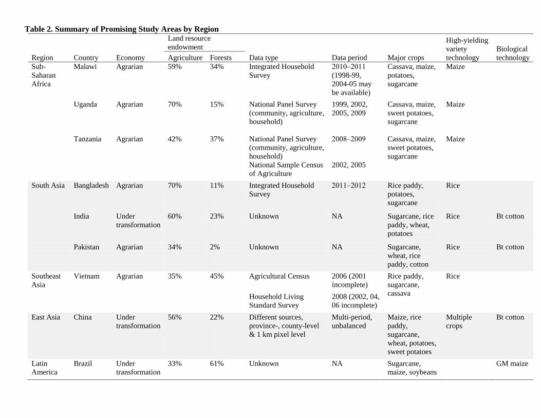
Table 2. Summary of Promising Study Areas by Region

Region Country Economy

Land resource

endowment

Data type Data period Major crops

High-yielding

variety

technology

Biological

technology Agriculture Forests

Sub-

Saharan

Africa

Malawi Agrarian 59% 34% Integrated Household

Survey

2010‒2011

(1998-99,

2004-05 may

be available)

Cassava, maize,

potatoes,

sugarcane

Maize

Uganda Agrarian 70% 15% National Panel Survey

(community, agriculture,

household)

1999, 2002,

2005, 2009

Cassava, maize,

sweet potatoes,

sugarcane

Maize

Tanzania Agrarian 42% 37% National Panel Survey

(community, agriculture,

household)

2008‒2009 Cassava, maize,

sweet potatoes,

sugarcane

Maize

National Sample Census

of Agriculture

2002, 2005

South Asia Bangladesh Agrarian 70% 11% Integrated Household

Survey

2011‒2012 Rice paddy,

potatoes,

sugarcane

Rice

India Under

transformation

60% 23% Unknown NA Sugarcane, rice

paddy, wheat,

potatoes

Rice Bt cotton

Pakistan Agrarian 34% 2% Unknown NA Sugarcane,

wheat, rice

paddy, cotton

Rice Bt cotton

Southeast

Asia

Vietnam Agrarian 35% 45% Agricultural Census 2006 (2001

incomplete)

Rice paddy,

sugarcane,

cassava

Rice

Household Living

Standard Survey

2008 (2002, 04,

06 incomplete)

East Asia China Under

transformation

56% 22% Different sources,

province-, county-level

& 1 km pixel level

Multi-period,

unbalanced

Maize, rice

paddy,

sugarcane,

wheat, potatoes,

sweet potatoes

Multiple

crops

Bt cotton

Latin

America

Brazil Under

transformation

33% 61% Unknown NA Sugarcane,

maize, soybeans

GM maize

References

1. Adams, R.M., Adams, D.M., Callaway, J.M., Chang, C.-c., McCarl, B.A., 1993.

Sequestering carbon on agricultural land: social cost and impacts on timber markets.

Contemporary Policy Issues 11, 76-87.

2. Adams, D. M., R.J. Alig, B.A. McCarl, J.M. Callaway, S.M. Winnett, Minimum cost

strategies for sequestering carbon in forests, Land Econ. 75 (3) (1999) 360–374.

3. Alig, R., Adams, D.M., McCarl, B.A., Callaway, J.M., Winnett, S., 1997. Assessing

effects of mitigation strategies for global climate change with an intertemporal model of

the U.S. forest and agriculture sectors. Environmental and Resource Economics 9, 259-

274.

4. Anderson, G. D., Opaluch, J. J., and W. M. Sullivan. 1985. "Nonpoint Agricultural

Pollution: Pesticide Contamination of Groundwater Supplies." Amer. J. Agr. Econ. 67:

1238-43.

5. Antle, J., S. Capalbo, K. Paustian, and M. Ali. 2007. Estimating the economic potential

for agricultural soil carbon sequestration in the Central United States using an aggregate

econometric-process simulation model. Climate Change 80: 145–171.

6. Antle, J., S. Capalbo, S. Mooney, E. Elliott, K. Paustian, Spatial heterogeneity, contract

design, and the efficiency of carbon sequestration policies for agriculture, J. Environ.

Econ. Manage. 42 (2) (2003) 231–250.

7. Antle, J.M., Diagana, B., 2003. Creating incentives for the adoption of sustainable

agricultural practices in developing countries: the role of soil carbon sequestration.

American Journal of Agricultural Economics 85, 1178-1184.

31

8. Babcock, B.A., and D.A. Hennessy. 1996. “Input Demand Under Yield and Revenue

Insurance.” American Journal of Agricultural Economics 78:416–27.

9. Blackorby, C., and W. Schworm. “The Existence of Input and Output Aggregates in

Aggregate Production Functions.” Econometrica 56(May 1988): 613-643.

10. Bouzaher, A., J.B. Braden, and G.V. Johnson. "A Dynamic Programming Approach to a

Class of Nonpoint Source Pollution Control Problems." Manage. Sci. 36(January

1990):1-15.

11. Braden, J.B., G.V. Johnson, A. Bouzaher, and D. Miltz. "Optimal Spatial Management of

Agricultural Pollution." Amer. J. Agr. Econ. 71(May 1989):404-13.

12. Brouwer, F. M., Thomas, A. J., and M. J. Chadwick. 1991. Land Use Changes in Europe:

Processes of Change, Environmental Transformations and Future Patterns: A study

initiated and sponsored by the International Institute for Applied Systems Analysis with

the support and co-ordination of the Stockholm Environment Institute. Dordrecht;

Boston: Kluwer Academic Publishers.

13. Capalbo, S.M., Antle, J.M., Mooney, S., Paustian, K., 2004. Sensitivity of carbon

sequestration costs to economic and biological uncertainties. Environmental Management

33, S238-S251.

14. Capozza, D. R., and R. W. Helsley. 1990. “The Stochastic City.” Journal of Urban

Economics 28: 187-03.

15. Caswell, M., and D. Zilberman. "The Choice of Irrigation Technologies in California."

Amer. J. Agr. Econ. 67(May 1985):224-34.

16. Chambers, R.G., and R.D. Pope. “Testing for Consistent Aggregation.” American

Journal of Agricultural Economics 73(August 1991): 808-18.

32

17. Chavas, J.P., and M.T. Holt. "Acreage Decisions Under Risk: The Case of Corn and

Soybeans." Amer. J. Agr. Econ. 72(August 1990):529-38.

18. Chavas, J.P., R.D. Pope, and R.S. Kao. "An Analysis of the Role of Future Prices, Cash

Prices, and Government Programs in Acreage Response." W. J. Agr. Econ. 8(July

1983):27-33.

19. Chavas, J.P., and K. Segerson. "Singularity and Autoregressive Disturbances in Linear

Logit Models." J. Bus. and Econ. Statist. 4(April 1986):161-69.

20. Chiappori, P.-A. “Distribution of Income and the "Law of Demand".” Econometrica

53(January 1985): 109-27.

21. Considine, T.J. "Symmetry Constraints and Variable Returns to Scale in Logit Models."

J. Bus. and Econ. Statist. 8(July 1990):347-53.

22. Considine, T.J., and T.D. Mount. "The Use of Linear Logit Models for Dynamic Input

Demand Systems." Rev. Econ. and Statist. 66(August 1984):434-43.

23. Cooper, J.C., and R.W. Keim. "Incentive Payments to Encourage Farmer Adoption of

Water Qual-ity Practices." Amer J. Agr. Econ. 78(Febru-ary 1996):54-64

24. Cropper, M., and C. Griffiths. "The Interaction of Population Growth and Environmental

Quality." The American Economic Review 84, Papers and Proceedings (May 1994): 250-

254.

25. Czech, B., P.R. Krausman, and P.K. Devers. “Economic Associations among Causes of

Species Endangerment in the United States.” BioScience 50 (2000): 593-601.

26. Deacon, R.T. "Deforestation and the Rule of Law in a Cross-Section of Countries." Land

Economics 70(November 1994): 414-430.

33

27. Deaton, M. L., and J. J. Winebrake. 2000. Dynamic Modeling of Environmental Systems.

New York: Springer-Verlag.

28. DeRoo, H.C. 1980. “Fluctuations in Ground Water as Influenced by Use of Fertilizer.”

Bulletin No. 779. June 1980. Connecticut Agricultural Experiment Station, New Haven,

Connecticut.

29. Duke, J., and J. Wu. Forthcoming. Oxford Handbook of Land Economics. Oxford, UK:

Oxford University Press.

30. Feng, H., Kurkalova, L.A., Kling, C.L., Gassman, P.W., 2006. Environmental

conservation in agriculture: land retirement vs. changing practices on working land.

Journal of Environmental Economics and Management 52, 600-614.

31. Friesen, L.E., P.F.J. Eagles, and R.J. Mackay. “Effects of Residential Development on

Forest-Dwelling Neotropical Migrant Songbirds.” Conservation Biology 9(6) (1995):

1408-1414.

32. Fuglie, K.O., and D.J. Bosch. "Economic and En-vironmental Implicationo f Soil

NitrogenT est-ing: A Switching-Regression Analysis."A mer. J. Agr. Econ. 77(November

1995):891-900.

33. Gilliam, J.W., and G.D. Hoyt. 1987. Effect of conservation tillage on fate and transport

of nitrogen. p. 217-40. In T.J. Logan, J.M. Davidson, J.L. Baker, and M.R. Overcash

(ed.) Effects of conservation tillage on groundwater quality: nitrates and pesticides.

Lewis Publishers, Inc. Chelsea, MI.

34. Gorman, W. M. “Community Preference Fields.” Econometrica 21(January 1953): 63-

80.

34

35. Goetz, W.J., C.R. Harper, C.E. Willis, and J.T. Finn. "Effects of Land Uses and

Hydrologic Characteristics on Nitrate and Sodium in Groundwater." Final Report for

Water Resources Research Center, University of Massachusetts, Project No. G1568-04,

January 1991.

36. Goss, D., and R.D. Wauchope. "The SCS/ARS/CES Pesticide Properties Database II:

Using it with Soils Data in a Screening Procedure." Pesticides in the Next Decade: The

Challenges Ahead. D. Weigeman, ed. Blacksburg VA: Virginia Water Resources

Research Center, 1991. Great Plains Agricultural Council, Water Quality Task Force.

Agriculture and Water Quality in the Great Plains: Status and Recommendations.

Publication No. 140, January 1992.

37. Green, R.C. Program Provisions for Program Crops: A Database for 1961-90.

Washington DC: U.S. Department of Agriculture, Agriculture and Trade Analysis

Division, ERS Staff Report No. AGES 9010, March 1990.

38. Greene, W.H. Econometric Analysis. New York: Macmillan, 1990.

39. Gupta, K.L. “Aggregation Bias in Linear Economics Models.” International Economic

Review 12(1971):293-305.

40. Hallberg, G.R. 1989. Nitrate in ground water in the united states. p. 35-74. In R.F. Follet

(ed.) Nitrogen management and ground-water protection. Elsevier Science Publishing

Co. New York.

41. Hardie, I., Parks, P. (1997) Land use with heterogeneous land quality: An application of

an area base model, American Journal of Agricultural Economics, 79: 299–310.

42. Hardie, W., T. A. Narayan, A. Tulika, and B. L. Gardner. “The Joint Influence of

Agricultural and Nonfarm Factors on Real Estate Values: An Application to the Mid-

35

Atlantic Region.” American Journal of Agricultural Economics 83 (February 2001): 120-

132.

43. Hascic, Ivan, and JunJie Wu. "Land Use and Watershed Health in the United States."

Land Economics 82(May 2006): 214-239.

44. Helfand, G.E., and B.W. House. “Regulating Nonpoint Source Pollution Under

Heterogeneous Conditions.” American Journal of Agricultural Economics

77(1995):1024–32.

45. Hildenbrand, W. “On the "Law of Demand.” Econometrica 51(July 1983): 997-1020.

46. Hochman, E., and D. Zilberman. "Examination of Environmental Policies Using

Production and Pollution Microparameter Distribution." Econometrica 46(July

1978):739-60.

47. Horowitz, J.K., and E. Lichtenburg. 1993. “Insurance, Moral Hazard, and Chemical Use

in Agriculture.” American Journal of Agricultural Economics 75: 926–35.

48. Houck, J.P., M.E. Abel, M.E. Ryan, P.W. Gallagher, R.G. Hoffman, and J.B. Penn.

Analyzing the Impact of Government Programs on Crop Acre-age. Washington DC: U.S.

Department of Agriculture Tech. Bull. 11548, August 1976.

49. Houck, J.P., and M.E. Ryan. "Supply Analysis for Corn in the United States: The Impact

of Changing Government Programs." Amer. J. Agr. Econ. 54(May 1972):184-91.

50. Huang, W.-Y., D. Westernbarger, and K. Mizer. 1992. The magnitude and distribution

of u.s. cropland vulnerable to nitrate leaching. In Making Information Work:

Proceedings, National Governors Association Conference, Washington D.C.

36

51. Irwin, E. G. and N. E. Bockstael. “Interacting Agents, Spatial Externalities, and the

Evolution of Residential Land Use Patterns.” Journal of Economic Geography 2 (2002):

31-54.

52. Irwin, E., K.P. Bell, N.E. Bockstael, D. Newburn, M.D. Partridge, and J. Wu. “The

Economics of Urban-Rural Space.” Annual Review of Resource Economics 1(October

2009): 1-26.

53. Irwin, E., and D. Wrenn. Forthcoming. “An Assessment of Empirical Methods for

Modeling Land Use.” In the Oxford Handbook of Land Economics. Oxford, UK: Oxford

University Press.

54. Johansen, L. Production Functions: An Integration of Micro and Macro, and Short Run

and Long Run Aspects. Amsterdam: North-Holland, 1972.

55. Johnson, S.L., R.M. Adams, and G.M. Perry. "The On-Farm Costs of Reducing

Groundwater Pollution." Amer. J. Agr. Econ. 73(November 1991):1063-73.

56. Judge, G.G., R.C. Hill, W.E. Griffiths, H. Lutkepohl, and T.C. Lee. Introduction to the

Theory and Practice of Econometrics, 2nd ed. New York: John Wiley & Sons, 1988.

57. Just, R., and J. Antle. "Interactions Between Agricultural and Environmental Policies: A

Concep-tual Framework." Amer. Econ. Rev. 80(May 1990):197-202.

58. Just, R., and N. Bockstael, eds. Commodity and Resource Policies in Agricultural

Systems. Berlin: Springer-Verlag, 1991.

59. Kellogg, R.L., M.S. Maizel, and D.W. Goss. 1992. Agricultural chemical use and

ground water quality: where are the potential problem areas? USDA Staff Rep., Soil

Conservation Service/Economic Research Service, Washington, D.C.

37

60. Kennedy, P. A Guide to Econometrics, 2nd ed. Cambridge MA: The MIT Press, 1990.

Kmenta, J. Elements of Econometrics. New York: Macmillan, 1986.

61. Klaiber, H. A., & Phaneuf, D. (2010). Valuing Open Space in a Residential Sorting

Model of the Twin Cities. Journal of Environmental Economics and Management , 60,

57-77.

62. Klaiber, H. Allen, and Nicolai V. Kuminoff. Forthcoming. “Equilibrium Sorting Models

of Land Use and Residential Choice.” In the Oxford Handbook of Land Economics.

Oxford, UK: Oxford University Press.

63. Klein, H.A.J. “Macroeconimics and the Theory of Rational Behavior.” Econometrica

14(January 1946): 93-108.

64. Langpap, Christian, Ivan Hascic, and JunJie Wu. “Protecting Watershed Ecosystems

through Targeted Local Land Use Policies.” American Journal of Agricultural Economics

90(August 2008): 684-700.

65. Langpap, Christian, and JunJie Wu. “Potential Environmental Impacts of Increased

Reliance on Corn-Based Bioenergy.” Environmental and Resource Economics 49(2011):

147-171.

66. Laws, E. A. 1993. Aquatic Pollution, An Introductory Text. 2nd ed. New York: Wiley.

67. Lawrence, C.L., and B.R. Ellefson. "Water Use in Wisconsin, 1979." U.S. Geological

Survey, Water Resources Investigations, 82-444, July 1982.

68. Lee, K.C., M.H. Pesaran, R.G. Pierse. “Testing for Aggregation Bias in Linear Models.”

The Economic Journal 100(Conference 1990):137-150.

38

69. Li, Man, JunJie Wu, Xiangzheng Deng. “Identifying Drivers of Land Use Change in

China: A Spatial Multinomial Logit Model Analysis.” Land Economics 89(November

2013): 632-654.

70. Lichtenberg, E. "Land Quality, Irrigation Development, and Cropping Patterns in the

Northern High Plains." Amer. J. Agr. Econ. 71(February 1989):187-94.

71. Lidman, R., and D.L. Bawden. "The Impact of Government Programs on Wheat

Acreage." Land Econ. 50(November 1974):327-35.

72. Love, H.A. “Conflicts Between Theory and Practice in Production Economics.” Paper

presented at the American Social Science Association Meeting, New York, New York,

January 1999.

73. Lubowski, R.N., Plantinga, A.J., Stavins, R.N. (2006) Land-use change and carbon sinks:

Econometric estimation of the carbon sequestration supply function, Journal of

Environmental Economics and Management, 51: 135–152.

74. Lutton, T.J., and M.R. LeBlanc. "A Comparison of Multivariate Logit and Translog

Models for Energy and Nonenergy Input Cost Share Analysis." Energy J. 5(October

1984):35-44.

75. Malmqvist, B., and S. Rundle. 2002. “Threats to the Running Water Ecosystems of the

World.” Environmental Conservation 29(2): 134-53.

76. Mapp, H.P., D.J. Bernardo, G.J. Sabbagh, S. Geleta, and B. Watkins. "Economic and

Environmental Impacts of Limiting Nitrogen Use to Protect Water Quality: A Stochastic

Regional Analysis." Amer. J. Agr. Econ. 76(November 1994):889-903.

77. Matson, P.A., W.J. Parton, A.G. Power, M.J. Swift. 1997. “Agricultural intensification

and ecosystem properties.” Science 277: 504-509.

39

78. McDonnell, J.J. (PD), et al. (2010). “Collaborative Research WSC Category 2:

Anticipating Water Scarcity and Informing Integrative Water System Response in the

Pacific Northwest.” A propose submitted to the National Science Foundation CR-Water

Sustainability & Climate.

79. Montgomery, C. A., R. A. Pollak; K. Freemark; D. White. “Pricing Biodiversity.”

Journal of Environmental Economics and Management, 38(1) (1999): 1-19.

80. Moore, M.R., and D.H. Negri. "A Multicrop Production Model of Irrigated Agriculture,

Applied to Water Allocation Policy of the Bureau of Reclamation." J. Agr. Resour. Econ.

17(July 1992):29-43.

81. Moulton, R. and Richards, K.: 1990, Costs of Sequestering Carbon through Tree Planting

and Forest Management in the United States, General Technical Report WO-58, U.S.

Department of Agriculture, Washington, D.C.

82. Muellbauer, J. “Aggregation, Income Distribution and Consumer Demand.” Review of

Economic Studies 42(October 1975): 525-543.

83. Neilson, R.P., and D. Marks. 1994. “A Global Perspective of Regional Vegetation and

Hydrologic Sensitivities from Climate Change.” Journal of Vegetation Science 5: 715-

730.

84. Nielsen, E.G., and L.K. Lee. "The Magnitude and Costs of Groundwater Contamination

from Ag-ricultural Chemicals: A National Perspective." U.S. Department of Agriculture,

ERS Agricultural Economic Report No. 576, October 1987.

85. Noss, R.R. Recharge Area Land Use and Well Water Quality. Progress Report. Amherst

MA: The En-vironmental Institute, University of Massachusetts, April 1988.

40

86. Opaluch, J.J., and K. Segerson. "Aggregate Analysis of Site-Specific Pollution Problems:

the Case of Groundwater Contamination From Agricultural Pesticides." Northeast. J.

Agr. Res. Econ. 20(April 1991):83-97.

87. Parker, D. C., S. M. Manson, M. A. Janssen, M. Hoffmann, and P. Deadman. 2003.

Multi-agent systems for the simulation of land-use and land-cover change: A review.

Annals of the Association of American Geographers 93(2): 314–337.

88. Parks, P.J., hardie, I.W., 1995. Least-cost forest carbon reserves: cost-effective subsidies

to convert marginal agricultural land to forests. Land Economics 71, 122-136.

89. Paustian, K., H. Collins, and E. Paul. 1997. Management controls on soil carbon, in Soil

Organic Matter in Temperate Agroecosystems: Long-Term Experiments in North

America. E. Paul, K. Paustian, E. Elliot, and C. Cole (eds.). pp 15–49. CRC Press, Boca

Raton, FL.

90. Pesaran, M.H., R.G. Pierse, and K.C. Lee. “Choice Between Disaggregate and

Aggregate Specifications Estimated by Instrumental Variables Methods.” Journal of

Business and Economic Statistics 12(January 1994):11-21.

91. Petr, F.C., and J.E. Bremer. "Keys to Profitable Corn Production in the High Plains."

Texas Agricultural Extension Service, Texas A&M University, 1976.

92. Pionke, H.B., and J.B. Urban. "Effect of Agricultural Land Use on Ground-Water Quality

in Small Pennsylvania Watershed." Ground Water 23(January-February 1985):68-80.

93. Piper, S., W.Y. Huang, and M. Ribaudo. "Farm Income and Ground water Quality

Implications From Reducing Surface Water Sediment Deliveries." Water Resour. Bull.

25(December 1989):1217-30.

41

94. Pimm, S.L., Russell, G.J., Gittleman, J.L., Brooks, T.M. (1995). “The future of

biodiversity”. Science 269, 347–350.

95. Plantinga, A.J., Mauldin, T., Miller, D.J., 1999. An econometric analysis of the costs of

sequestering carbon in forests. American Journal of Agricultural Economy 81, 812-824.

96. Plantinga, A.J., and J. Wu. "Co-Benefits from Carbon Sequestration in Forests:

Evaluating Reductions in Agricultural Externalities from an Afforestation Policy in

Wisconsin." Land Economics 79(Feburary 2003):74-85.

97. Richards, K.R., Stokes, C., 2004. A review of forest carbon sequestration cost studies: a

dozen years of research. Climatic Change 63, 1-48.

98. Rothman, D.S., J.H. Hong, and T.D. Mount. "Estimating Consumer Energy Demand

Using International Data: Theoretical and Policy Implications." Working Paper 93-10,

Department of Agricultural Economics, Cornell University, July 1993.

99. Rothschild, E.R., R.J. Manser, and M.P. Anderson. "Investigation of Aldicarb in Ground

Water in Selected Areas of the Central Sand Plain of Wisconsin." Ground Water 20(July-

August 1982):437-45.

100. Rottenborn, S.C. “Predicting the Impacts of Urbanization on Riparian Bird

Communities.” Biological Conservation 88 (1999): 289-299.

101. Ryszkowski, L. 2002. Landscape Ecology in Agroecosystems Management. Boca Raton,

FL: CRC Press.

102. Sasaki, K. “An Empirical Analysis of Linear Aggregation Problems: The Case of

Investment Behavior in Japanese Firms.” Journal of Econometrics 7(1978):313-331.

103. Schindler, D. W. 1977. “Evolution of Phosphorus Limitation in Lakes.” Science 195: 260

-62.

42

104. Sedjo, R.A. 1993. “The Carbon Cycle and Global Forest Ecosystems.” In J. Wisniewski

and R.N. Sampson (eds.), Terrestrial Biospheric Carbon Fluxes: Quantification of Sinks

and Sources of CO2. Boston: Kluwer Academic Publishers, 295-309.

105. Sedjo, R.A., J. Wisniewski, A.V. Sample, and J.D. Kinsman. "The Economics of

Managing Carbon via Forestry: Assessment of Existing Studies." Environmental and

Resource Economics 6(September 1995):139-165.

106. Segerson, K. "Incentive Policies for Control of Agricultural Water Pollution."

Agriculture and Water Quality: International Perspectives. John B. Braden and Stephen

B. Lovejoy, eds. Boulder CO: Lynne Rienner Publishers, 1990.

107. Segerson, K., and J. Wu. "Economic Analysis and Groundwater Quality: A Survey of

Related Re-search." Working paper, Department of Economics, University of

Connecticut, September 1994. Shumway, C.R. "Supply, Demand, and Technology in a

Multiproduct Industry: Texas Field Crops." Amer. J. Agr. Econ. 65(November

1983):748- 60.

108. Shumway, C.R. 1983. “Supply, Demand, and Technology in a Multiproduct Industry:

Texas Field Crops.” American Journal of Agricultural Economics 65: 748-760.

109.

110. Simmons, P., and D. Weiserbs. "Translog Flexible Functional Forms and Associated

Demand Systems." Amer. Econ. Rev. 69(December 1979):892-901.

111. Smith, R.A., R.B. Alexander, and M.G. Wolman. 1987. Water quality trends in the

nation’s rivers. Science 235:1607-15.

43

112. Sohngen, B., and R. Alig. "Mitigation, Adaption, and Climate Change: Results from

Recent Research on the U.S. Forest Sector." Environmental Science and Policy 3

(2000):235-248.

113. Sohngen, B., and R. Sedjo. 2000. “Potential Carbon Flux from Timber Harvests and

Management in the Context of a Global Timber Market.” Climatic Change 44: 151-172.

114. ———. 2006. “Carbon Sequestration in Global Forests Under Different Carbon Price

Regimes” in The Energy Journal, Special issue, Multi-Greenhouse Gas Mitigation and

Climate Policy, pps. 109-162, December.

115. Stavins, R.N., 1999. The costs of carbon sequestration: a revealed-preference approach,

Amer. Econ. Rev. 89 (4): 994–1009.

116. Stavins, R., Jaffe, A. (1990) Unintended impacts of public investments on private

decisions: The depletion of forested wetlands, The American Economic Review, 80: 337–

352.

117. Stavins, R.N., 1999. The costs of carbon sequestration: a revealed-preference approach.

The American Economic Review 89, 994-1009.

118. Stiegler, J.H. "Cropping Systems and Rotations." Wheat and Wheat Improvement, 2nd

ed. E.G. Heyne, ed., pp. 325-29. Madison WI: American Society of Agronomy, 1987.

119. Stoker, T.M. “Completeness, Distribution Restrictions, and the Form of Aggregate

Functions.” Econometrica 52(July 1984): 887-907.

120. Tanaka, Katsuya, and JunJie Wu. “Evaluating the Effect of Conservation Policies on

Agricultural Land Use: A Site-Specific Modeling Approach.” Canadian Journal of

Agricultural Economics 52(November 2004).

44

121. Theil, H. "A Multinomial Extension of the Linear Logit Model." Int. Econ. Rev.

10(October 1969):251-59. Tyrrell, T., and T. Mount. "A Nonlinear Expenditure System

Using a Linear Logit Specification." Amer. J. Agr. Econ. 64(August 1982):539-45.

122. Tilman, D., K.G. Cassman, P.A. Matson, R. Naylor, S. Polasky. 2002. “Agricultural

sustainability and intensive production practices.” Nature 418: 671-677.

123. U.S. Department of Agriculture, Statistical Reporting Service. Agricultural Statistics.

Washington DC, 1971-90. U.S. Geological Survey, U.S. Geological Service. National

Water Summary 1986-Hydrologic Events and Groundwater Quality. Washington DC,

USGS Water-Supply Papers, pp. 531-37, 1988.

124. Vroomen, H., and B. Larson. A Direct Approach for Estimating Nitrogen, Phosphorus,

and Land Demands at the Regional Level. Washington DC: U.S. Department of

Agriculture, ERS Technical Bulletin No.1786, March 1989.

125. Wales, T.J. "On the Flexibility of Flexible Functional Forms: An Empirical Analysis." J.

Econometrics 5(March 1977):183-93.

126. Walsh, R. (2007). Endogenous Open Space Amenities in a Locational Equilibrium.

Journal of Urban Economics , 61, 319-344.

127. Watanabe, Michio, Richard M. Adams, and JunJie Wu. “The Economics of

Environmental Management in a Spatially Heterogeneous River Basin.” American

Journal of Agricultural Economics 88(August 2006): 617-631.

128. Weaver, R.D. "Multiple Input, Multiple Output Production Choices and Technology in

the U.S. Wheat Region." Amer. J. Agr. Econ. 65(February 1983):45-56.

129. White, D., P. G. Minotti, M. J. Barczak, J. C. Sifneos, K. E. Freemark, M. V.

Santelmann, C. F. Steinitz, A. R. Kiester, and E. M. Preston. “Assessing Risks to

45

Biodiversity from Future Landscape Change.” Conservation Biology 11(2) (1997): 349-

360.

130. Willis, R.J., and S. Rosen. "Education and Self- Selection." J. Polit. Econ. 87(No. 2,

1979): S7-S36.

131. Wu, J. 1999. “Crop Insurance, Acreage Decisions, and Nonpoint-Source Pollution.”

American Journal of Agricultural Economics 81:305–20.

132. Wu, JunJie, and Richard A. Adams. “Micro vs. Macro Acreage Response Models: Does

Site-Specific Information Matter?” Journal of Agricultural and Resource Economics

27(July 2002):40-60.

133. Wu, JunJie, Richard M. Adams, Catherine L. Kling, and Katsuya Tanaka. “From Micro-

Level Decisions to Landscape Changes: An Assessment of Agricultural Conservation

Policies.” American Journal of Agricultural Economics 86(February 2004): 26-41.

134. Wu, JunJie, and Richard M. Adams “Production Risk, Acreage Decisions, and

Implications for Revenue Insurance Programs” Canadian Journal of Agricultural

Economics 49(March 2001): 19-35.

135. Wu, JunJie, and Seong-Hoon Cho. “The Effect of Local Land Use Regulations on Urban

Development in the Western United States.” Regional Science and Urban Economics

37(2007): 69-86.

136. Wu, JunJie, and Bruce A. Babcock. "Metamodeling Potential Nitrate Water Pollution in

the Central United States." Journal of Environmental Quality 28(November-December

1999): 1916-1928.

46

137. Wu, JunJie, and Bruce A. Babcock. “The Choice of Tillage, Rotation, and Soil Testing

Practices: Economic and Environmental Implications.” American Journal of Agricultural

Economics 80(August 1998):494-511.

138. Wu, JunJie, D.J. Bernardo, H.P. Mapp, S. Geleta, M.L. Teague, K.B. Bradley, G.J.

Sabbagh, R.L. Elliott, and J.H. Stone. "An Evaluation of Nitrogen Runoff and Leaching

Potential in the High Plains." Journal of Soil and Water Conservation (January-February

1997): 73-80.

139. Wu, JunJie, and B. Wade Brorsen. "The Impact of Government Programs and Land

Characteristics on Cropping Patterns." Canadian Journal of Agricultural Economics

43(March 1995):87-104.

140. Wu, JunJie, Monica Fisher, and Unai Pascual. “Urbanization and the Viability of Local

Agricultural Economies.” Land Economics 87(February 2011): 109-125.

141. Wu, Junjie, and Katsuya Tanaka. “Reducing Nitrogen Runoff from the Upper

Mississippi River Basin to Control Hypoxia in the Gulf of Mexico: Easements or Taxes?”

Marine Resource Economics 20, 2(July 2005): 121-144.

142. Wu, JunJie, and Kathleen Segerson. "The Impact of Policies and Site Characteristics on

Potential Groundwater Pollution in Wisconsin." American Journal of Agricultural

Economics 77 (November 1995):1033-47.

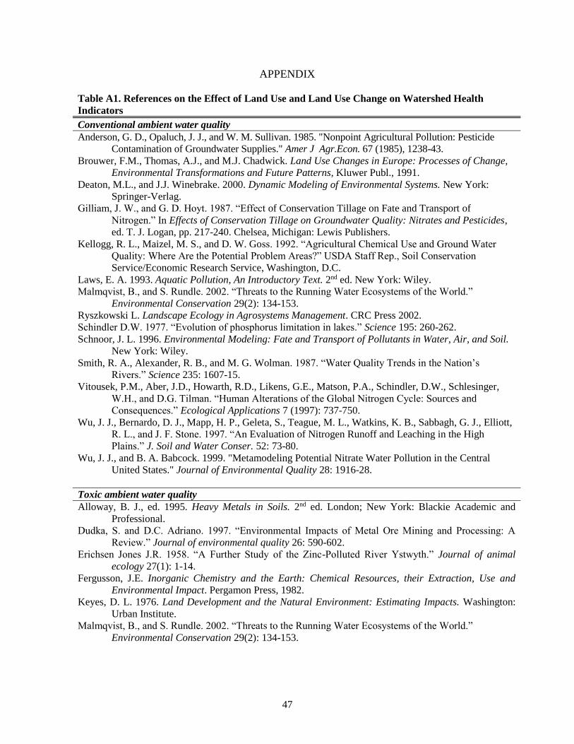
47

APPENDIX

Table A1. References on the Effect of Land Use and Land Use Change on Watershed Health

Indicators

Conventional ambient water quality

Anderson, G. D., Opaluch, J. J., and W. M. Sullivan. 1985. "Nonpoint Agricultural Pollution: Pesticide

Contamination of Groundwater Supplies." Amer J Agr.Econ. 67 (1985), 1238-43.

Brouwer, F.M., Thomas, A.J., and M.J. Chadwick. Land Use Changes in Europe: Processes of Change,

Environmental Transformations and Future Patterns, Kluwer Publ., 1991.

Deaton, M.L., and J.J. Winebrake. 2000. Dynamic Modeling of Environmental Systems. New York:

Springer-Verlag.

Gilliam, J. W., and G. D. Hoyt. 1987. “Effect of Conservation Tillage on Fate and Transport of

Nitrogen.” In Effects of Conservation Tillage on Groundwater Quality: Nitrates and Pesticides,

ed. T. J. Logan, pp. 217-240. Chelsea, Michigan: Lewis Publishers.

Kellogg, R. L., Maizel, M. S., and D. W. Goss. 1992. “Agricultural Chemical Use and Ground Water

Quality: Where Are the Potential Problem Areas?” USDA Staff Rep., Soil Conservation

Service/Economic Research Service, Washington, D.C.

Laws, E. A. 1993. Aquatic Pollution, An Introductory Text. 2nd ed. New York: Wiley.

Malmqvist, B., and S. Rundle. 2002. “Threats to the Running Water Ecosystems of the World.”

Environmental Conservation 29(2): 134-153.

Ryszkowski L. Landscape Ecology in Agrosystems Management. CRC Press 2002.

Schindler D.W. 1977. “Evolution of phosphorus limitation in lakes.” Science 195: 260-262.

Schnoor, J. L. 1996. Environmental Modeling: Fate and Transport of Pollutants in Water, Air, and Soil.

New York: Wiley.

Smith, R. A., Alexander, R. B., and M. G. Wolman. 1987. “Water Quality Trends in the Nation’s

Rivers.” Science 235: 1607-15.

Vitousek, P.M., Aber, J.D., Howarth, R.D., Likens, G.E., Matson, P.A., Schindler, D.W., Schlesinger,

W.H., and D.G. Tilman. “Human Alterations of the Global Nitrogen Cycle: Sources and

Consequences.” Ecological Applications 7 (1997): 737-750.

Wu, J. J., Bernardo, D. J., Mapp, H. P., Geleta, S., Teague, M. L., Watkins, K. B., Sabbagh, G. J., Elliott,

R. L., and J. F. Stone. 1997. “An Evaluation of Nitrogen Runoff and Leaching in the High

Plains.” J. Soil and Water Conser. 52: 73-80.

Wu, J. J., and B. A. Babcock. 1999. "Metamodeling Potential Nitrate Water Pollution in the Central

United States." Journal of Environmental Quality 28: 1916-28.

Toxic ambient water quality

Alloway, B. J., ed. 1995. Heavy Metals in Soils. 2nd ed. London; New York: Blackie Academic and

Professional.

Dudka, S. and D.C. Adriano. 1997. “Environmental Impacts of Metal Ore Mining and Processing: A

Review.” Journal of environmental quality 26: 590-602.

Erichsen Jones J.R. 1958. “A Further Study of the Zinc-Polluted River Ystwyth.” Journal of animal

ecology 27(1): 1-14.

Fergusson, J.E. Inorganic Chemistry and the Earth: Chemical Resources, their Extraction, Use and

Environmental Impact. Pergamon Press, 1982.

Keyes, D. L. 1976. Land Development and the Natural Environment: Estimating Impacts. Washington:

Urban Institute.

Malmqvist, B., and S. Rundle. 2002. “Threats to the Running Water Ecosystems of the World.”

Environmental Conservation 29(2): 134-153.

48

McGowen, S. L., and N. T. Basta. 2001. “Heavy Metal Solubility and Transport in Soil Contaminated by

Mining and Smelting.” In: Heavy Metals Release in Soils. eds. Selim, H. M., and D. L. Sparks.

Boca Raton, Florida: Lewis Publ.

Novotny V. and Olem H. Water Quality: Prevention, Identification, and Management of Diffuse Pollution.

Van Nostrand Reinhold, New York, 1994.

Stephenson, T. 1987. “Sources of Heavy Metals in Wastewater.” In Heavy Metals in Wastewater and

Sludge Treatment Processes, vol. 1, Sources, Analysis, and Legislation. ed. J. N. Lester. Boca

Raton, Florida: CRC Press.

Aquatic and wetland species at risk of extinction

Angermeier, P. L. 1995. “Ecological Attributes of Extinction-Prone Species: Loss of Freshwater Species

of Virginia.” Conservation Biology 9(1): 143-158.

Carpenter, S. R., Caraco, N. F., Correll, D. L., Howarth, R. W., Sharpley, A. N., and V. H. Smith. 1998.

“Nonpoint Pollution of Surface Waters with Phosphorus and Nitrogen.” Ecological Applications

8(3): 559-568.

Czech, B., Krausman, P. R., and P. K. Devers. 2000. “Economic Associations among Causes of Species

Endangerment in the United States.” BioScience 50: 593-601.

Frissell, C. A. 1993. “Topology of Extinction and Endangerment of Native Fish in the Pacific Northwest

and California (U.S.A.),” Conservation Biology 7(2): 342-354.

Handy, R. D., and F. B. Eddy. 1990. “The Interactions between the Surface of Rainbow Trout,

Oncorhynchus Mykiss, and Waterborne Metal Toxicants (in Freshwater).” Functional Ecology

4(3) New Horizons in Ecotoxicology pp.385-392.

Harding, J. S., Benfield, E. F., Bolstad, P. V., Helfman, G. S., and E. B. D. Jones. 1998. “Stream

Biodiversity: The Ghost of Land Use Past.” Proceedings of the National Academy of Sciences of

the United States of America 95:25.

Laws, E. A. 1993. Aquatic Pollution, An Introductory Text. 2nd ed. New York: Wiley.

Mason, C. F. 1977. “Populations and Productions of Benthic Animals in Two Contrasting Shallow Lakes

in Norfolk.” Journal of Animal Ecology 46(1): 147-172.

Richter, B. D., Braun, D. P., Mendelson, M. A., and L. L. Master. 1997. “Threats to Imperiled Freshwater

Fauna.” Conservation Biology 11(5): 1081-93.

Sayer, C., Roberts, N., Sadler, J., David, C., and P. M. Wade. 1999. “Biodiversity Changes in a Shallow

Lake Ecosystem: A Multi-Proxy Palaeolimnological Analysis.” Journal of Biogeography 26(1):

97-114.

Schindler, D. W. 1990. “Experimental Perturbations of Whole Lakes as Tests of Hypotheses Concerning

Ecosystems Structure and Function.” Oikos 57: 25-41.

Seehausen, O. J., van Alpen, J. M., and F. Witte. 1997. “Cichlid Fish Diversity Threatened by

Eutrophication that Curbs Sexual Selection.” Science 277: 1808-11.

Skidmore, J. F. 1964. “Toxicity of Zinc Compounds to Aquatic Animals, with Special Reference to

Fish.” Quarterly Review of Biology 39(3): 227-248.

Smith, V. H. 1998. “Cultural Eutrophication of Inland, Estuarine, and Coastal Waters.” In: Successes,

Limitations, and Frontiers in Ecosystem Science. eds. Pace, M.L., and P.M. Groffman. New

York: Springer-Verlag.

Vitousek, P. M., Aber, J. D., Howarth, R. D., Likens, G. E., Matson, P. A., Schindler, D. W., Schlesinger,

W. H., and D. G. Tilman. 1997. “Human Alterations of the Global Nitrogen Cycle: Sources and

Consequences.” Ecological Applications 7: 737-750.

Winston, M.R., Taylor, C.M., and J. Pigg. 1991. “Upstream Extirpation of Four Minnow Species due to

Damming of a Prairie Stream.” Transactions of the American Fisheries Society 120: 98-105.

Source: Hascic and Wu (2006)