Landau damping - SMAIsmai.emath.fr/cemracs/cemracs10/PROJ/Villani-lectures.pdfLandau damping Cédric Villani Ecole Normale Sup´ érieure de Lyon & Institut Henri Poincaré, 11

Landau damping

Cedric Villani

Ecole Normale Superieure de Lyon & Institut Henri

Poincare, 11 rue Pierre et Marie Curie, F-75231 Paris Cedex

05, FRANCE

E-mail address : [email protected]

Contents

Foreword 7

Chapter 1. Mean field approximation 91. The Newton equations 92. Mean field limit 103. Precised results 144. Singular potentials 15Bibliographical notes 17

Chapter 2. Qualitative behavior of the Vlasov equation 191. Boundary conditions 192. Structure 203. Invariants and identities 214. Equilibria 235. Speculations 24Bibliographical notes 25

Chapter 3. Linearized Vlasov equation near homogeneity 290. Free transport 291. Linearization 322. Separation of modes 333. Mode-by-mode study 354. The Landau–Penrose stability criterion 385. Asymptotic behavior of the kinetic distribution 426. Qualitative recap 43Bibliographical notes 45

Chapter 4. Nonlinear Landau damping 471. Nonlinear stability? 472. Elusive bounds 483. Backus’s objection 484. Numerical simulations 495. Theorem 496. The information cascade 53Bibliographical notes 55

1

2 CONTENTS

Chapter 5. Gliding analytic regularity 571. Preliminary analysis 572. Algebra norms 583. Gliding regularity 614. Functional analysis 62Bibliographical notes 63

Chapter 6. Characteristics in damped forcing 651. Damped forcing 652. Scattering 66Bibliographical notes 68

Chapter 7. Reaction against an oscillating background 691. Regularity extortion 692. Solving the reaction equation 703. Analysis of the kernel K 724. Analysis of the integral equation 745. Effect of singular interactions 766. Large time estimates via exponential moments 78Bibliographical notes 80

Chapter 8. Newton’s scheme 810. The classical Newton scheme 811. Newton scheme for the nonlinear Vlasov equation 832. Short time estimates 843. Large time estimates 864. Main result 93Bibliographical notes 93

Chapter 9. Conclusions 95Bibliographical notes 96

Bibliography 99

Abstract. These notes constitute an introduction to the Landaudamping phenomenon in the linearized and perturbative nonlinearregimes, following the recent work [74] by Mouhot & Villani.

3

Foreword

In 1936, Lev Landau devised the basic collisional kinetic modelfor plasma physics, now commonly called the Landau–Fokker–Planckequation. With this model he was introducing the notion of relaxationin plasma physics: relaxation a la Boltzmann, by increase of entropy,or equivalently loss of information.

In 1946, Landau came back to this field with an astonishing concept:relaxation without entropy increase, with preservation of information.The revolutionary idea that conservative phenomena may exhibit ir-reversible features has been extremely influential, and later led to theconcept of violent relaxation.

This idea has also been controversial and intriguing, triggering hun-dreds of papers and many discussions. The basic model used by Landauwas the linearized Vlasov–Poisson equation, which is only a formal ap-proximation of the Vlasov–Poisson equation. In the present notes Ishall present the recent work by Clement Mouhot and myself, extend-ing Landau’s results to the nonlinear Vlasov–Poisson equation in theperturbative regime. Although this extension is still far from handlingthe mysterious fully nonlinear regime, it already turned out to be richand tricky, from both the mathematical and the physical points of view.

These notes start with basic reminders about classical particle sys-tems and Vlasov equations, assuming no prerequisite from modelingnor physics. Standard notation is used throughout the text, exceptmaybe for the Fourier transforms: if h = h(x, v) is a function on the

position-velocity phase space, then h stands for the Fourier transform

in the x variable only, while h stands for the Fourier transform in bothx and v variables. Precise conventions will be given later on.

This course was first taught in the summer of 2010 in Cotonou,Benin, on the invitation of Wilfrid Gangbo; and in Luminy, France,on the invitation of Eric Sonnendrucker. It is a pleasure to thank theaudience for their interest and enthusiasm. Typing was mostly per-formed in the welcoming library of the gorgeous Domaine des Treilles

7

8 FOREWORD

of the Fondation Schlumberger, whose hospitality is gratefully acknowl-edged, during a meeting on wave turbulence organized by ChristopheJosserand.

CHAPTER 1

Mean field approximation

The two main classes of kinetic equations are the collisional equa-tions of Boltzmann type, modeling short-range interactions, and themean field equations of Vlasov type, modeling long-range interactions.The disinction between short-range and long-range does not refer tothe decay of the microscopic interaction, but to the fact that the rele-vant interaction takes place at distances which are much smaller than,or comparable to, the macroscopic scale; in fact both types of interac-tion may occur simultaneously. Collisional equations are discussed inmy survey [99]. In this chapter I will concisely present the archetypalmean field equations.

1. The Newton equations

The collective interaction of a large population of “particles” arisesin a number of physical situations. The basic model consists in thesystem of Newton equations in Rd (typically d = 3):

(1.1) mi xi(t) =∑

j

Fj→i(t),

where mi is the mass of particle i, xi(t) ∈ Rd its position at time t, xi(t)its acceleration, and Fj→i is the force exerted by particle j on particlei. Even if this model does not take into account quantum or relativisticeffects, huge theoretical and practical problems remain dependent onour understanding of (1.1).

The masses in (1.1) may differ my many orders of magnitude; ac-tually this disparity of masses plays a key role in the study of the solarsystem, or the Kolmogorov–Arnold–Moser theory [27], among otherthings. But it also often happens that the situation where all massesmi are equal is relevant, at least qualitatively. In the sequel, I shallonly consider this situation, so mi = m for all i.

If the interaction is translation invariant, it is often the case that thethe force derives from an interaction potential: there is W : Rd → R

such that

F = −∇W (x− y)

9

10 1. MEAN FIELD APPROXIMATION

is the force exterted at position x by a particle located at position y.This formalism misses important classes of interaction such as magneticforces, but it will be sufficient for our purposes.

Examples 1.1. (a) W (x−y) = const. ρ ρ′/|x−y| is the electrostaticinteraction potential between particles with respective electric chargesρ and ρ′, where |x− y| is the Euclidean distance in R3; (b) W (x− y) =−const. mm′/|x− y| is the gravitational interaction potential betweenparticles with respective masses m and m′, also in R3; (c) Essentiallyany potential W arises in some physical problem or the other, and evena smooth (or analytic!) interaction potential W leads to relevant anddifficult problems.

As an example, let us write the basic equation governing the posi-tions of stars in a galaxy:

xi(t) = G∑

j 6=i

mjxj − xi

|xj − xi|3,

where G is the gravitational constant. Note that in this example, a staris considered as a “particle”! There are similar equations describingthe behavior of ions and electrons in a plasma, involving the dielectricconstant, mass and electric charges.

In the sequel, I will assume that all masses are equal and work inadimensional units, so masses will not explicitly appear in the equa-tions.

But now there are as many equations as there are particles, andthis means a lot. A galaxy may be made of N ≃ 1013 stars, a plasmaof N ≃ 1020 particles... thus the equations are untractable in practice.Computer simulations, available on Internet, give a flavor of the richand complex behavior displayed by large particle systems interactingthrough gravity. It is very difficult to say anything intelligent in frontof these complex pictures. This complex behavior is partly due to thefact that the gravitational potential is attractive and singular at theorigin; but even for a smooth interaction W would the large value ofN cause much trouble in the quantitative analysis.

The mean field limit will lead to another model, more amenableto mathematical treatment.

2. Mean field limit

The limit N → ∞ allows to replace a very large number of simpleequations by just one complicated equation. Although we are tradingreassuring ordinary differential equations for dreaded partial differen-tial equations, the result will be more tractable.

2. MEAN FIELD LIMIT 11

From the theoretical point of view, the mean field approximation isfundamental: not only because it establishes the basic limit equation,but also because it shows that the qualitative behavior of the systemdoes not depend much on the exact value of the number of particles,and then in numerical simulations for instance we can replace trillionsof particles by, say, millions or even thousands.

It is not a priori obvious how one can let the dimension of the phasespace go to infinity. As a first step, let us double variables to convertthe second-order Newton equations into a first-order system. So foreach position variable xi we introduce the velocity variable vi = xi

(time-derivative of the position), so that the whole state of the systemat time t is described by (x1, v1), . . . , (xN , vN). Let us write Xd for thed-dimensional space of positions, which may be Rd, or a subset of Rd,or the d-dimensional torus Td if we are considering periodic data; thenthe space of velocities will be Rd.

Since all particles are identical, we do not really care about the stateof each particle individually: it is sufficient to know the state of thesystem up to permutation of particles. In slightly pedantic terms, we aretaking the quotient of the phase space (Xd ×Rd)N by the permutationgroup SN , thus obtaining a cloud of undistinguishable points.

There is a one-to-one correspondence between such a cloud C =(x1, v1), . . . , (xN , vN) and the associated empirical measure

µN =1

N

N∑

i=1

δ(xi,vi),

where δ(x,v) is the Dirac mass in phase space at (x, v). From the physicalpoint of view, the empirical measure counts particles in phase space.

Now the empirical measure µN belongs to the space P (Xd × Rd),the space of probability measures on the single-particle phase space.This space is infinite-dimensional, but it is independent of the numberof particles. So the plan is to re-express the Newton equations in termsof the empirical measure, and then pass to the limit as N → ∞.

For simplicity I shall assume that Xd is either Rd or Td, and thatthe force derives from an interaction potential W . The following propo-sition, slightly informal, establishes the link between the Newton equa-tions and the empirical measure equation.

Proposition 1.2. (i) Let W ∈ C1(Xd; R), and for each i let xi =xi(t); then with the notation µN = N−1

∑δ(xi,xi) the following two


statements are equivalent:

(1.2) ∀i, xi = −c∑

j

∇W (xi − xj)

(1.3)∂µN

∂t+ v · ∇xµ

N + FN(t, x) · ∇vµN = 0,

where

FN(t, x) = −c∑

j

∇W (x− xj) = −cN(∇W ∗x,v µ

N).

(ii) If ∇W is uniformly continuous and µN0 converges weakly to

some measure µ0 and c = c(N) satisfies cN → γ ≥ 0 as N → ∞,then up to extraction of a subsequence, µN converges as t → ∞ to atime-dependent measure µ = µt(dx dv) solving the system

(1.4)

∂µ

∂t+ v · ∇xµ+ F (t, x) · ∇vµ = 0

F = −γ∇W ∗x,v µ

Remark 1.3. Equations (1.3) and (1.4) are to be understood indistributional sense, that is, after integrating on the phase space againsta nice test function ϕ(x, v), say smooth and compactly supported. Torewrite these equations in distributional form, note that

v · ∇xµ = ∇x · (vµ), F (t, x) · ∇vµ = ∇v ·(F (t, x)µ

).

(To be rigorous one should also use a test function in time, but this isnot a serious issue and I shall leave it aside.)

Remark 1.4. The second formula in (1.4) can be made more ex-plicit as

F (t, x) = −∫∫

W (x− y)µt(dy dw);

of course the convolution in the velocity variable is trivial since ∇Wdoes not depend on it; so this is just an integration in velocity space.

Remark 1.5. By definition, a sequence of measures µN converges toa measure µ in the weak sense if, for any bounded continuous functionϕ(x, v),

∫∫ϕ(x, v)µN(dx dv) −−−→

N→∞

∫∫ϕ(x, v)µ(dx dv).

If µN and µ are probability measures, then weak convergence is equiv-alent to convergence in the sense of distributions.

2. MEAN FIELD LIMIT 13

Sketch of proof of Proposition 1.2. Let us forget about is-sues of regularity and well-posedness, and focus on the core compu-tations, assuming that xi(t) is a smooth function of t. When we testequation (1.3) against an arbitrary function ϕ = ϕ(x, v) we obtain

d

dt

[1

N

∑

i

ϕ(xi, vi)

]− 1

N

∑

i

(v · ∇xϕ)|(xi,vi)− 1

N

∑

i

(FN · ∇vϕ)∣∣(xi,vi)

= 0,

where the time-dependence is implicit; by chain-rule this means

1

N

∑

i

(∇xϕ · xi + ∇vϕ · vi −∇xϕ · vi −∇vϕ · FN(xi)

)= 0,

where ϕ inside the summation is evaluated at (xi, vi). Since vi = xi,this equation reduces to

(1.5)1

N

∑

i

[vi − FN(t, xi)

]· ∇vϕ(xi, vi) = 0.

Now this should hold true for any test function ϕ(x, v). Choosing onewhich takes the form e · v near (xi, vi) (with e an arbitrary vector) andwhich vanishes near (xj, vj) for all j 6= i, we deduce that vi = FN(t, xi).(This argument is not fully rigorous since it may happen that twodistinct particles occupy similar positions in phase space, but that isnot a big deal to fix.) Now (1.5) is just a way to rewrite (1.2); theequivalence between (1.2) and (1.3) follows easily.

Next we note that∑

∇W (x− xj) = N∇W ∗ µ, where the convo-lution is in both variables x and v. In retrospect, it is normal that theforce should be expressed in terms of the empirical measure, since thisis a symmetric expression of the positions of particles.

Now let us consider the limit N → ∞. Let us fix a finite time-horizon T > 0 and work on the time-interval [−T, T ]. By assumptionthe initial data µN(0, ·) form a tight family; then from the differentialequation satisfied by the measures µN(t, · ) it is not difficult to showthat µN(t, · ) is also tight, uniformly in t ∈ [−T, T ]. Then, up to extrac-tion of a subsequence, µN(t, ·) will converge in C([−T, T ];D′(Xd×Rd))for any T > 0, to some limit measure µ(t, dx dv). It only remains topass to the limit in the equation.

Being the convolution of a uniformly continuous function with aprobability measure, hte force field FN = −cN ∇W ∗ µN is uniformlycontinuous on [−T, T ] × Xd, and will converge uniformly as N → ∞to −γ∇W ∗ µ. This easily implies that

FN µN −→ F µ


in distributional sense, whence ∇v · (FN µN) −→ ∇v · (F µ). Similarly,∇x · (vµN) converges to ∇x · (vµ), and the proof is complete.

The limit equation (1.4) is called the nonlinear Vlasov equation

associated with the interaction potential W . It makes sense just aswell for µt(dx dv) = N−1

∑δ(xi(t),vi(t)) (in which case it reduces to the

Newton dynamics) as for µt(dx dv) = f(t, x, v) dx dv, that is, for a con-tinuous distribution of matter. In fact the nonlinear Vlasov equationis the completion, in the space of measures, of the system of Newtonequations.

It is customary and physically relevant to restrict to the case of acontinuous distribution function, and then focus on the equation satis-fied by f(t, x, v). Since the Lebesgue measure dx dv is transparent tothe differential operators ∇x and ∇v, one easily obtains the nonlinear

Vlasov equation for the density function f = f(t, x, v):

(1.6)

∂f

∂t+ v · ∇xf + F (t, x) · ∇vf = 0

F = −∇W ∗x ρ, ρ(t, x) =

∫f(t, x, v) dv,

where the (x, v)-convolution has been explicitly replaced by a convolu-tion in x and an integration in v.

Equation (1.6) is the single most important partial differential equa-tions of mean field systems, and will be the object of study of thiscourse.

3. Precised results

In Proposition 1.2 it was assumed that W is continuously differen-tiable. If W is smoother then one can prove more precise results ofquantitative convergence, involving distances on probability measures,for instance the Wasserstein distances Wp. For the present section, itwill be sufficient to know the 1-Wasserstein distance, defined by theformula

W1(µ, ν) := sup

∫ψ dµ−

∫ψ dν; ‖ψ‖Lip ≤ 1

,

where the supremum is over all 1-Lipschitz functions ψ of (x, v), andit is assumed that µ and ν possess a finite moment of order 1. (If oneimposes that ψ is also bounded in supremum norm, one obtains theclosely related “bounded Lipschitz” distance, which does not need anymoment assumption.)

Here is a typical estimate of convergence for the mean-field limit,stated here without proof, going back to Dobrushin:

4. SINGULAR POTENTIALS 15

Proposition 1.6. If µt(dx dv) and νt(dx dv) are two solutions ofthe nonlinear Vlasov equation with interaction potential W , then forany t ∈ R

(1.7) W1(µt, νt) ≤ e2C|t|W1(µ0, ν0), C = max(‖∇2W‖L∞, 1

).

It might not be obvious why this provides a convergence estimatein the mean-field limit. To see this, choose µt(dx dv) = f(t, x, v) dx dvand νt = µN

t ; then (1.7) controls at time t the distance between thelimit mean-field behavior and the Newton equation for N particles, interms of how small this distance is at initial time t = 0. If the particlesat t = 0 are chosen randomly, then typically the W1 distance at t = 0is O(1/

√N), so W1(µt, νt) = O(e2C|t|/

√N), which solves the problem.

(Note that this estimate requires crazy amounts of particles to get agood precision in large time.)

Another type of estimates are large deviation bounds:

Proposition 1.7. If ∇2W is bounded, f0 = f0(x, v) is given with∫∫f0(x, v) e

β(|x|2+|v|2) dx dv ≤ C0, (xi(0), xi(0)), 1 ≤ i ≤ N , are chosenrandomly and independently according to f0(x, v) dx dv, (xi(t)) solvethe Newton equations (1.2) with c = 1/N , and f(t, x, v) solves thenonlinear Vlasov equation (1.6), then there is K > 0 such that for anyT ≥ 0 there is C = C(T ) such that

(1.8) N ≥ N0 max(ε−(2d+3), 1

)=⇒

P

[sup

0≤t≤TW1

(µN

t , f(t, x, v) dx dv)> ε

]≤ C

(1 + ε−2

)e−KNε2

,

where P stands for probability.

Many refinements are possible: for instance, one can estimate thedensity error between f(t, x, v) and the empirical measure, after smooth-ing by a peaked convolution kernel; study the evolution of (de)correlationsbetween particles which are initially randomly distributed; show thattrajectories of particles in the system of size N are well approximatedby trajectories of particles evolving in the limit mean-field force, etc.

4. Singular potentials

Fine. But eventually, more often than not, the interaction potentialis not smooth at all, instead it is rather singular. Then nobody has aclue of why the mean-field limit should be true. The problem might bejust technical, but on the contrary it seems very deep.

Such is the case in particular for the most important nonlinearVlasov equations, namely the Vlasov–Poisson equations, where W


is the fundamental solution of ±∆. In dimension d = 3, writing r =|x− y|, we have

• the Coulomb interaction (repulsive) W =1

4πr;

• the Newton interaction (attractive) W = − 1

4πr.

Then the equation F = −∇W ∗ ρ becomes F = ±∇∆−1ρ.

It is remarkable that, up to a change of sign in the interaction, thevery same equation describes systems of such various scales as a plasmaand a galaxy, in which each star counts as one particle! In fact to bemore precise, we should slightly change the equation for plasmas, bytaking into account the contribution of heavy ions, which is usuallyconsidered in the form of a fixed density of positive charges, say ρI(x),and by considering magnetic effects, which in some situations play animportant role. Things become much more messy when irreversiblephenomena are taken into account, but these phenomena occur only ascorrections to the mean-field limit, due to the fact that N is finite.

While the mean-field limit for smooth potential has been well-understood for more than three decades, in the case of singular po-tentials the only available results are those obtained a few years agoby Hauray and Jabin: they assume that (a) the interaction is no toosingular: essentially |∇W | = O(r−s) with 0 < s < 1 (independently ofthe dimension d); and (b) particles are well-separated in phase spaceinitially, so

(1.9) infj 6=i

(|xi − xj | + |vi − vj|

)≥ c

N12d

,

where c is of course independent of N .Both conditions are not so satisfactory: assumption (a) misses the

Coulomb/Newton singularity by an order 1 + 0, while assumption (b)cannot be true in the simplest case when particles are chosen randomlyand idependently of each other. It might be that assumption (b) can begiven a physical justification, though, based on the ionization processfor instance; but that remains to be done. For numerical purpose, as-sumption (b) is more satisfactory since we can choose the discretizationas we wish.

In any case, a key ingredient in the proof of the Hauray–Jabintheorem consists in showing that the separation (1.9) property is prop-agated in time: if true at t = 0, it remains true for later times, upto a deterioration of constants. This implies that the proportion ofparticles located in a box of side ε in phase space remains bounded likeO(ε2d) as time goes by, uniformly in N . (This is a discrete analogue

BIBLIOGRAPHICAL NOTES 17

of the property of propagation of L∞ bounds for the nonlinear Vlasovequation, which will be examined in the next chapter)

What about the theory of the nonlinear Vlasov equation? Is thesystem well-posed for a given initial datum? For smooth interactionsthis does not pose any problem, but when the interaction potentialis singular, this becomes highly nontrivial. Most efforts have beenfocused on the Poisson coupling in dimension 3. Although this maynot have been considered carefully, the theory would probably workjust the same in arbitrary dimensions and with a coupling that is nomore singular than Poisson. There are two famous theories for theVlasov–Poisson equation with large data:

• The Pfaffelmoser theory, developed and simplified in particularby Batt, Rein, Glassey, Scheffer, construct smooth solutions assumingessentially that fi is C1 and compactly supported in (x, v).

• The Lions–Perthame theory constructs a unique solution for aninitial datum fi on R3

x × R3v which satisfies, say,

(1.10) |fi(x, v)| + |∇f(x, v)| ≤ C

(1 + |x| + |v|)10.

(The exponent 10 depends on the fact that dimension is 3, and anywayshould not be taken seriously.) Besides velocity averaging phenomena,the key insight of the analysis is the propagation of bounds on velocitymoments of order greater than 3. Then one can show that the spatialdensity is uniformly bounded, and the smoothness is propagated too.

Both theories are still incomplete. The Lions–Perthame theorytakes advantage of the dispersion at large positions to control velocity-moments; it has never been checked that it can be adapted in boundedgeometries, like the torus T3. As for the Pfaffelmoser theory, it doesadapt to bounded geometries, but the assumption of compact supportin the velocity space, is a heresy, since it does not include even the sin-gle most important distribution in kinetic theory, namely the Gaussiandistribution.

Perturbative theories of the nonlinear Vlasov equation near an equi-librium are in better shape. We shall see an example in this course.This suggests that the problem of the mean-field limit in a perturbativesetting could be attacked.

Bibliographical notes

Impressive particle simulations of large systems, performed by JohnDubinski, can be found online at www.galaxydynamics.org


The kinetic theory of plasmas was born in Soviet Union in the thir-ties, when Landau adapted the Boltzmann collision operator to theCoulomb interaction [55] and Vlasov argued that long-range interac-tions should be taken into account by a conceptually simpler mean-fieldterm [103]. The collisional kinetic theory of plasmas is described ina number of physics textbooks [1, 54, 61] and in the mathematicalreview [99]; see also [2, Sections 1 and 2].

The mean field limit however did not become a mathematical sub-ject until the classical works by Dobrushin [31], Braun & Hepp [20],and Neunzert [77]. Braun & Hepp were also interested in the propaga-tion of chaos and the study of fluctuations; these topics are addressedagain in Sznitman’s Saint-Flour lecture notes [95]. Other syntheticsources are the book by Spohn [92] and my incomplete lecture noteson the mean field limit [102], which both contain a recast of the proofof Proposition 1.6. Quantitative estimates of the mean field limit forsimple (stochastic) models and smooth interaction are found in mywork [15] joint with Bolley and Guillin; the proof of Proposition 1.7can be obtained by adapting the estimates therein.

The mean-field limit for mildly singular interactions was consideredby Hauray and Jabin [42] in a pioneering work that still needs to bedigested and simplified by the mathematical community.

Early contributions to the Cauchy problem for the Vlasov–Poissonequation, working either in short time, or with weak solutions, or insmall dimension, are due to Arsen’ev, Horst, Bardos, Degond, Bena-chour, DiPerna & Lions in the seventies and eighties [6, 7, 9, 12, 28,

46, 47]. The theory reached a more mature stage with the ground-breaking works by Pfaffelmoser [83] and Lions & Perthame [60] atthe dawn of the nineties. Pfaffelmoser’s approach was simplified bySchaeffer [90] and Horst [48], and is well exposed by Glassey [35]; theadaptation to periodic data was performed by Batt & Rein [10]. Thealternative Lions–Perthame approach is presented by Bouchut [17].

CHAPTER 2

Qualitative behavior of the Vlasov equation

In the previous chapter we were interested in the derivation andwell-posedness of the Vlasov equation

(2.1)

∂f

∂t+ v · ∇xf + F (t, x) · ∇vf = 0

F = −∇W ∗x ρ ρ(t, x) =

∫f(t, x, v) dv.

But now the emphasis will be different: starting from the Vlasov equa-tion, we shall enquire about its qualitative behavior. This problem fillsup textbooks in physics, and has been the subject of an enormousamount of literature.

1. Boundary conditions

There is a zoology of boundary conditions for the Vlasov equation.To avoid discussing them, I shall continue to assume that the positionspace is either Xd = Rd, the whole space, or Xd = Td/Zd, the d-dimensional torus. The latter case deserves some comments.

If W is a given potential in Rd, then in the periodic setting, formallyW should be replaced by its periodic version W per:

W per(x) =∑

k∈Zd

W (x− k).

If W decays fast enough, this is well-defined, but if W has slow decay,like in the case of Poisson interaction, this will not converge! Thenthe justification requires some argument. In fact, it is clear that forPoisson coupling the potential cannot converge: in the case of thePoisson coupling, the total potential W ∗ ρ should formally be equal to±∆−1ρ, which does not make sense since ρ does not have zero mean...To get around this problem, we would like to take out the mean of ρ.

In the plasma case, one can justify this by going back to the model:indeed, one may argue that the density of ions should be taken intoaccount, that it can be modelled as a uniform background because ionsare much heavier and move on longer time scales than electrons, andthat the density of ion charges should be equal to the mean density of

19

20 2. QUALITATIVE BEHAVIOR OF THE VLASOV EQUATION

electrons because the plasma should be globally neutral. This amountsto replace the potential W ∗ ρ by W ∗ (ρ− 〈ρ〉), where 〈ρ〉 =

∫ρ dx.

The preceding reasoning is based on the existence of two differentspecies of particles. But even if there is just one species of particles, asis the case for gravitational interaction, it is still possible to argue thatthe mean should be removed. Indeed, in (2.1) W only appears throughits gradient, and, whenever c is a constant,

∇W ∗ (ρ− c) = ∇W ∗ ρ−∇W ∗ c = ∇W ∗ ρ.Thus, if W decays fast enough at infinity and ρ is periodic,

∇W ∗ ρ = ∇W per ∗ ρ = ∇W per ∗ (ρ− 〈ρ〉).If W does not decay fast enough at infinity, then at least we can writeW = limε→0Wε, where Wε is an approximation decaying fast at infinity(say ±e−r/ε/(4πr), then ∇Wε ∗ ρ = ∇W per

ε ∗ (ρ − 〈ρ〉), which in thelimit ε → 0 converges to ∇W per ∗ (ρ − 〈ρ〉). Of course this might notbe so convincing in the absence of a clear discussion of the meaning ofthe parameter ε, but at least makes sense in some regime and allowsto take out the mean 〈ρ〉 from the density in (2.1). This operation issimilar to the so-called Jeans swindle in astrophysics.

Having warned the reader that there is a subtle point here, from nowon in the periodic setting I shall always write ∇W ∗ρ for ∇W ∗(ρ−〈ρ〉).As a final comment, one may argue against the relevance of periodicboundary conditions, especially in view of the above discussion; but thisis still by far the simplest way to have access to a confined geometry,avoiding effects such as dispersion at infinity which completely changethe qualitative behavior of the nonlinear Vlasov equation.

2. Structure

The nonlinear Vlasov equation is a transport equation, and cantherefore be solved by the well-known method of characteristics: iff solves the equation, then the measure f(t, x, v) dx dv is the push-

forward of the initial measure fi(x, v) dx dv by the flow S0,t = (Xt, Vt)in phase space, solving the characteristic equations

Xt = Vt, Vt = F (t, Xt), F = −∇W ∗ ρ,

(X0, V0) = (x, v).

Of course this does not solve the problem “explicitly”, since the force Fat time t depends on the whole distribution of particles via the formulaF = −∇W ∗ (

∫f dv).

3. INVARIANTS AND IDENTITIES 21

Recall that the push-forward of a measure µ0 by a map S is definedby S#µ0[A] = µ0[S

−1(A)]. The resulting equation on the densities gen-erally involves the Jacobian determinant of the flow at time t. Howeverin the present case, the flow St induced by F (t, x) preserves the Liou-ville measure dx dv (that is a consequence from its Hamiltonian nature),so the push-forward equation can be simplified in a pull-back equationfor densities. In other words, the solution f(t, x, v) will satisfy

(2.2) f(t, S0,t(x, v)) = f(0, x, v).

Thus, to get the distribution function at time t we should invert themap St, in other words solve the characteristics backwards. If St,0

stands for the inverse of S0,t, then (2.2) becomes

(2.3) f(t, x, v, ) = f(0, St,0(x, v)).

Depending on situation, taste and theory, one considers the nonlin-ear Vlasov equation either from the Eulerian point of view (focus onf(t, x, v)), or from the Lagrangian point of view (focus on particle tra-jectories in a force field reconstructed from the particle distribution).This affects not only the theory, but also the numerics, since numer-ical methods may be Eulerian (look at values of f on a grid, say),or Lagrangian (consider particles moving), or semi-Lagrangian (makeparticles move and interpolate at each step to reconstruct values of fon a grid).

Apart from that, equation (2.1) is a limit of Hamiltonian equations(the Newton equations), and actually has a Hamiltonian structure ina certain sense, in relation with optimal transport theory; this linkwas explored in particular by Ambrosio, Gangbo and Lott. For themoment it is not clear whether this striking structure has physicallyrelevant implications beyond what is already known.

3. Invariants and identities

In this section I shall review the four main invariances and iden-tities associated with the nonlinear Vlasov equation, assuming thateverything is well-defined and being content with formal identities.

• The nonlinear Vlasov equation preserves the total energy∫∫

f(x, v)|v|22dx dv +

1

2

∫∫W (x− y) ρ(x) ρ(y) dx dy =: T + U

is constant in time along solutions. The total energy is the sum of thekinetic energy T and the potential energy U . (The factor 1/2 in thedefinition of U comes from the fact that we should count unorderedpairs of particles.)


• The nonlinear Vlasov equation preserves all the nonlinear inte-

grals of the density: often called the Casimirs of the equation, theytake the form ∫∫

A(f(x, v)) dx dv,

where A is arbitrary. These millions of conservation laws are imme-diately deduced from (2.3); in other words, they express the fact thatthe Vlasov equation induces a transport by a measure-preserving (infact Hamiltonian) flow. In particular, all Lp norms are preserved, thesupremum is preserved... and so is the entropy:

S = −∫∫

f log f dx dv.

The latter property is in sharp contrast with the Boltzmann equation,for which the entropy can only increase in time, unless it is at equilib-rium. Physically speaking, it reflects the preservation of information:whatever information we have about the distribution of particles atinitial time, is preserved at later times.

• The equation is time-reversible: choose an initial datum fi, letit evolve by the nonlinear Vlasov equation from time 0 to time T ,then reverse velocities (that is replace f(T, x, v) by f(T, x,−v)) let itevolve again for an additional time T , reverse velocities again, and youare back to the initial datum fi. This again is in contrast with thetime-irreversibility of the Boltzmann equation. As a consequence, thenonlinear Vlasov equation does not have any regularizing effect, at leastin the usual sense.

• The last identity is called the virial theorem; it only holds inthe whole space and for specific classes of interaction. The virial1 isdefined as

V =

∫∫f(x, v) x · v dx dv

is the time-derivative of the inertia

I =

∫∫f(x, v)

|x|22dx dv.

If the potential W is even and λ-homogeneous, that is, for any z ∈ Rd

and α 6= 0,

W (−z) = W (z), W (αz) = |α|λW (z),

1This word was made up by Clausius using the latine root for “force”.

4. EQUILIBRIA 23

then one has the virial identity

dVdt

= 2T − λU.

The most famous case of application is of course the case of Coulomb/Newtonequation, for which λ = −1, which yields

dVdt

= 2T + U.

When one takes a time-average and looks over large times, thecontribution of the time-derivative is likely to disappear, and we areleft with the plausible guess

(2.4) 2〈T 〉 + 〈U〉 = 0,

where 〈u〉 = limT→∞ T−1∫ T

0u(t) dt. Identity (2.4) suggests some kind

of biased, but universal partition between the kinetic and potentialenergies.

4. Equilibria

A famous property of the Boltzmann equation is that it only hasGaussian equilibria. In contrast, the Vlasov equation has infinitelymany shapes of equilibria.

First of all, any distribution f(x, v) = f 0(v) defines a spatially

homogeneous equilibrium. Indeed, v · ∇xf0 = 0, and the density

ρ0 associated to f 0 is constant, so the corresponding force vanishes(∇W ∗ ρ0 = W ∗ (∇ρ0) = 0).

The construction of other classes of equilibria is easy by meansof the so-called Jeans theorem: any function of the invariants of theflow is an equilibrium. As the most basic example, let us search for astationary f in the form of a function of the microscopic energy

E(x, v) =|v|22

+ Φ(x), Φ = W ∗ ρ,

where ρ =∫f dv. Using the ansatz f(x, v) = f(E), where f is an

arbitrary function R → R+, we get by chain-rule

v · ∇xf −∇Φ · ∇vf = (f)′(E)[v · ∇Φ −∇Φ · v

]= 0,

so f is an equilibrium.Of course this works only if the potential Φ is indeed induced by f ,

which leads to the compatibility condition∫f

( |v|22

+ Φ(y)

)W (x− y) dy dv = Φ(x).


For a given f this is a nonlinear integral equation on the unknown Φ;in the general case it is certainly too hard to solve, but if we are lookingfor solutions with symmetries, depending on just one parameter, thiscan often be done in practice.

If W is the Coulomb or Newton potential, the integral equationtransforms into a differential equation; as a typical situation, considerthe three-dimensional gravitational case with radial symmetry, then ρand Φ are functions of r, and we have after a few computations

ρ(r) = 4π

∫ 0

Φ(r)

√2(E − Φ(r)) f(E) dE.

This gives ρ as a function of Φ, and then the formulas for sphericalLaplace operator applied to radial functions yield

1

r2

d

dr(r2 Φ′(r)) = 4π ρ(Φ),

whence f(x, v) = f(|v|2/2 + Φ(r)) can be reconstructed.Another typical situation is the one-dimensional Coulomb interac-

tion with periodic data: then the equation is

−Φ′′(x) =

∫f

(v2

2+ Φ(x)

)− 1,

subject to the condition∫f(v2/2 + Φ(x)) dv = 1. Such a solution is

called a BGK equilibrium, after Bernstein, Greene and Kruzkal; orBGK wave, to emphasize the periodic nature of the solution. Suchwaves exist as soon as f is smooth and decays fast enough at infinity,and satisfies

∫f(v2/2) dv = 1.

5. Speculations

The general concern by physicists is about the large time asymp-totics, t→ ∞. Can one somehow draw a picture of the possible quali-tative behavior of solutions to the nonlinear Vlasov equations?

Usually a first step in the understanding of the large-time behav-ior is the identification of stable structures such as equilibria. In thepresent case, the abundance of equilibria is a bit disorienting, and wewould like to find selection criteria allowing to make predictions in largetime.

Are equilibria stable? There is a convincing stability criterion forhomogeneous equilibria, due to Penrose, which will be studied in Chap-ter 3. But no such thing exists for BGK waves, and nobody has a cluewhether these equilibria should be stable or unstable.


Having no convincing answer to the previous question, we may turnto an even more difficult question, that is, which equilibria are attrac-tive? Can one witness convergence to equilibrium even in the absenceof dissipative features in the equation? Does the Vlasov equation ex-hibit non-entropic relaxation, that is, relaxation without increaseof entropy? This has been the object of considerable debate, and sug-gested by numerical experiments on the one hand, observation on theother hand: as pointed out by the astrophysicist Lynden-Bell in the six-ties, galaxies, roughly speaking, seem to be in equilibrium at relevantscales, although the relaxation times associated with entropy produc-tion in galaxies exceed by far the age of the universe. Lynden-Bellargued that there should be a mechanism of violent relaxation, ofwhich nobody has a decent understanding.

If the final state is impossible to predict, maybe this problem canbe attacked in a statistical way: Lynden-Bell and followers argued thatsome equilibria, in particular those having high entropy, may be favoredby statistical considerations. Maybe there are invariant measures onthe space of solutions of the nonlinear Vlasov equation, which can beused to statistically predict the large-time behavior of solutions??

In all this maze of speculations, questions and religions, the onlytiny island on which we can stand on our feet is the Landau damp-

ing phenomenon: a relaxation property near stable equilibria, whichis driven by conservative phenomena. In the sequel I shall describethis phenomenon in great detail; for the moment let me emphasizethat besides its theoretical and practical importance by itself, it is theonly serious theoretical hint of the possibility of dissipation-free relax-ation in confined systems, without appealing to an extra randomnessassumption.


I am not aware of any good synthetic introductory source for bound-ary conditions of the nonlinear Vlasov equations; but this topic is dis-cussed for instance in the research paper [40]. Boundary conditionsfor kinetic equations are also evoked in [23, Chapter 8] or [99, Section1.5]. The Cauchy problem for Vlasov–Poisson in a bounded convexdomain is studied in [49]; for nonconvex domain it is expected thatserious issues arise about the regularity.

The Jeans swindle appears in many textbooks in astrophysics tojustify asymptotic expansions when the density is a perturbation ofa uniform constant in the whole space, see e.g. [14]. The underlyingmathematical meaning of the procedure is neatly explained by Kiessling


[52]. The explanations given in Section 1 are just an adaptation of theargument to the periodic situation.

The Hamiltonian nature of the nonlinear Vlasov equation, in re-lation with optimal transport theory, is discussed informally in myintroductory book on optimal transport [100, Section 8.3.2], and morerigorously by Ambrosio & Gangbo [4], and Lott [62, Section 6]. Some ofthese features are shared by other partial differential equations, in par-ticular the two-dimensional incompressible Euler equation, for which agood concise source is [68]. The similarity between the one-dimensionalVlasov equation and the two-dimensional Euler equation with nonneg-ative vorticity is well-known; physicists have systematically tried toadapt tools and theories from one equation to the other.

The statistical meaning of the entropy, and its relation to the Boltz-mann formula S = k logW is discussed in many sources; a conciseaccount can be found in my tribute to Boltzmann [101].

Formal properties of the Vlasov equation, including the virial the-orem, are covered in many textbooks such as Binney & Tremaine [14].This reference also discusses the procedure for constructing inhomoge-neous equilibria.

BGK waves were introduced in the seminal paper [13] and havebeen the object of many speculations in the literature; see [57, 58] fora recent treatment. No BGK wave has been proven to be stable withrespect to periodic perturbations (that is, whose period is equal to theperiod of the wave). The only known related statement is the instabilityagainst perturbations with period twice as long [57, 58]. (This holdsin dimension 1, but can probably be translated into a multidimensionalresult.) At least this means that a BGK wave f on T × R cannot behoped to be stable if f is 1/2-periodic in x.

The idea of violent relaxation was introduced in the sixties byLynden-Bell [63, 64], who at the same time founded the statisticaltheory of the Vlasov equation. The theory has been pushed by severalauthors, and also adapted to the two-dimensional incompressible Eulerequation [24, 70, 87, 96, 97, 104]. Since it is based on purely heuris-tic grounds and on just the conservation laws satisfied by the Vlasovequation (not on the equation itself), the statistical theory has beenthe object of criticism, see e.g. [51].

The construction of invariant measures on infinite-dimensional Hamil-tonian systems has failed for classical equations such as the Vlasov or(two-dimensional, positive vorticity, incompressible) Euler equations[85]; but it was solved for certain dispersive equations, such as thecubic nonlinear Schrodinger equations, treated by Bourgain [19]. As


far as the Vlasov or Euler equations are concerned, there is no canon-ical choice of what could be a Gibbs measure, but now there mightbe hope with Sturm’s construction of a fascinating canonical “entropicmeasure” on the space of probability measures [94], coming from thetheory of optimal transport. But for the moment very little is knownabout Sturm’s measure, and measures drawn according to this measureare not even absolutely continuous.

CHAPTER 3

Linearized Vlasov equation near homogeneity

Vlasov, Landau and other pioneers of kinetic theory of plasmasdiscovered a fundamental property: when one linearizes the Vlasovequation around a homogeneous equilibrium, the resulting linear equa-tion is “explicitly” solvable; in a way this is a completely integrable

system. This allowed Landau to solve the stability and asymptotic be-havior for the linearized equation — two problems which seem out ofreach now for inhomogeneous equilibria.

0. Free transport

As a preliminary, let us study the properties of free transport, thatis, when there is no interaction (W = 0):

(3.1)∂f

∂t+ v · ∇xf = 0.

The properties of this equation differ much in the whole space Rd

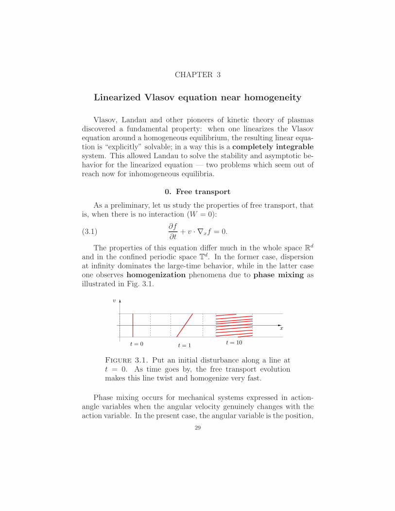
and in the confined periodic space Td. In the former case, dispersionat infinity dominates the large-time behavior, while in the latter caseone observes homogenization phenomena due to phase mixing asillustrated in Fig. 3.1.

v

t = 0 t = 1t = 10

x

Figure 3.1. Put an initial disturbance along a line att = 0. As time goes by, the free transport evolutionmakes this line twist and homogenize very fast.

Phase mixing occurs for mechanical systems expressed in action-angle variables when the angular velocity genuinely changes with theaction variable. In the present case, the angular variable is the position,

29

30 3. LINEARIZED VLASOV EQUATION NEAR HOMOGENEITY

so the angular velocity is the plain velocity, which coincides preciselywith the action variable.

t = 100

t = 0

t = 1

Figure 3.2. An example of a system which is not mix-ing: for the harmonic oscillator (linearized pendulum)the angular velocity is independent of the action vari-able, so a disturbance in phase space keeps the sameshape as time goes by.

The free transport equation can be solved explicitly (which shouldnot prevent us from keeping the qualitative picture in mind): if fi isthe datum at t = 0, then

(3.2) f(t, x, v) = fi(x− vt, v)

To study fine properties of this solution, it is most convenient touse the Fourier transform. Let us introduce the position-velocityFourier transform

f(k, η) =

∫∫f(x, v) e−2iπk·x e−2iπη·v dx dv,

where k ∈ Zd is dual to x ∈ Td, and η ∈ Rd is dual to v ∈ Rd. Then(3.2) implies

f(t, k, η) =

∫∫fi(x− vt, v) e−2iπk·x e−2iπη·v dx dv(3.3)

=

∫∫fi(x, v) e

−2iπk·(x+vt) e−2iπη·v dx dv(3.4)

= fi(k, η + kt).(3.5)

We deduce that

• f(t, 0, η) = fi(0, η): the zero spatial mode of f is preserved;

0. FREE TRANSPORT 31

• for fixed η and k 6= 0, fi(k, η + kt) −→ 0 as t → ∞, at arate which is (a) determined by the smoothness of fi in v(Riemann–Lebesgue lemma), (b) faster when k is large. In fact, the relevant timescale for the mode k is |k|t.

In particular, if fi is analytic in v then fi decays exponentiallyfast in η, so the mode k of the solution of the free transport equationwill decay like O(e−2πλ|k|t). Also, if f is only assumed to be Sobolevregular, say W s,1 in the velocity variable for some s > 0, then theFourier transform will decay like O(|η|−s) at large values of |η|, so themode of order k will decay like O((|k|t)−s).

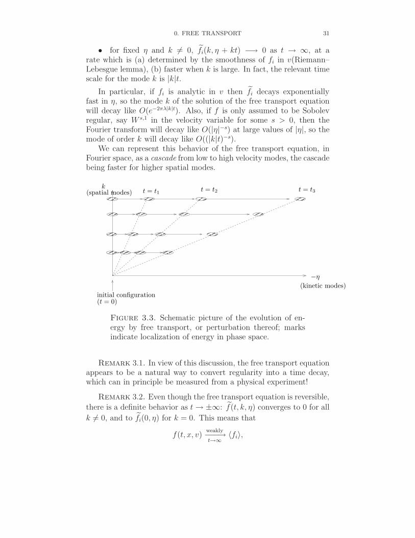
We can represent this behavior of the free transport equation, inFourier space, as a cascade from low to high velocity modes, the cascadebeing faster for higher spatial modes.

k

(kinetic modes)

initial configuration(t = 0)

(spatial modes) t = t1 t = t2 t = t3

−η

Figure 3.3. Schematic picture of the evolution of en-ergy by free transport, or perturbation thereof; marksindicate localization of energy in phase space.

Remark 3.1. In view of this discussion, the free transport equationappears to be a natural way to convert regularity into a time decay,which can in principle be measured from a physical experiment!

Remark 3.2. Even though the free transport equation is reversible,

there is a definite behavior as t→ ±∞: f(t, k, η) converges to 0 for all

k 6= 0, and to fi(0, η) for k = 0. This means that

f(t, x, v)weakly−−−→t→∞

〈fi〉,


where the brackets stand for spatial average:

〈h〉(v) =

∫h(x, v) dx.

The convergence holds as long as the initial measure does have a den-sity, that is, fi is well-defined as an integrable function; and it is fasterif fi is smooth.

Remark 3.3. Why don’t we see such phenomena as recurrence,which are associated with confined mechanical systems? The answeris that as soon as the distribution is spread out and has a density,we do not expect such phenomena because the system truly is infinite-dimensional. Recurrence would occur with a singular distribution func-tion, say Dirac masses, but we ruled out this situation.

1. Linearization

Now let us go back to the Vlasov equation. Let f 0 = f 0(v) bea homogeneous equilibrium. We write f(t, x, v) = f 0(v) + h(t, x, v),where ‖h‖ ≪ 1 in some sense. Since f 0 does not contribute to theforce field, the nonlinear Vlasov equation becomes

∂h

∂t+ v · ∇xh+ F [h] · ∇v(f

0 + h) = 0,

where

F [h](t, x) = −∫∫

∇W (x− y) h(t, y, w) dy dw = −∇xW ∗x,v h.

When h is very small we expect the quadratic term F [h] · ∇vh tobe negligible in front of the linear terms, and obtain

(3.6)∂h

∂t+ v · ∇xh+ F [h] · ∇vf

0 = 0.

The physical interpretation of (3.6) is not so obvious. Assume thatwe have two species of particles, one that has distribution h and theother one that has distribution f 0, and that the h-particles act on thef 0-particles by forcing, still they are unable to change the distributionf 0 (like you are pushing a wall, to no effect). In this case, we canimagine that the changes in the f 0 density would be compensated bythe transmutation of h-particles into f 0-particles, or the reverse. Thenthe equation for f 0 will be

(3.7) F [h] · ∇vf0 = S,

2. SEPARATION OF MODES 33

where S is the source of f 0 particles, and thus the equation for h wouldbe

(3.8)∂h

∂t+ v · ∇xh = −S.

The combination of (3.7) and (3.8) implies (3.6). Thus, in some sense,equation (3.6) can be interpreted as expressing the reaction exertedby the “wall” f 0 on the particle density.

We note that the last term on the right-hand side of (3.6) has theform F [h] · ∇vf

0, where F [h] is a function of t and x, and f 0(v) is afunction of v. This property of separation of variables will be crucial.As a start, it implies the statement below.

Proposition 3.4. If h = h(t, x, v) evolves according to the lin-earized Vlasov equation (3.6), then the function 〈h〉 =

∫h(t, x, v) dx

depends only on v and not on t.

An equivalent statement is that the linearized Vlasov equationhas an infinite number of conservation laws: for any function ψ(v),∫hψ dv dx is a conserved quantity.

Proof of Proposition 3.4. First note that 〈∇xh〉 = 0 and 〈F [h]〉 =0, since F [h] is a gradient. So (3.6) implies

∂t〈h〉 = −〈v · ∇xh〉 −⟨F [h] · ∇vf

0⟩

= −v · ∇x〈h〉 − 〈F [h]〉 · ∇vf0 = 0.

2. Separation of modes

Let us now work on the linearized equation, in the form

(3.9)∂h

∂t+ v · ∇xh+ F [h] · ∇vf

0 = 0.

Solving this equation is a beautiful exercice in linear partial differentialequations, involving three ingredients (whose order does not mattermuch): the method of characteristics, the integration in v, and theFourier transform in x.

• First step: the method of characteristics. We apply theDuhamel principle to (3.9), treating it as a perturbation of free trans-port. It is easily checked that the solution of ∂th+ v · ∇xh = −S takesthe form

h(t, x, v) = hi(x− vt, v) −∫ t

0

S(τ, x− v(t− τ), v) dτ,


where hi(x, v) = h(0, x, v).

• Second step: Fourier transform. Taking Fourier transformin both x and v yields

h(t, k, η) =

∫∫hi(x− vt, v) e−2iπk·x e−2iπη·v dx dv

(3.10)

−∫∫ ∫ t

0

S(τ, x− v(t− τ), v) e−2iπk·x e−2iπη·v dx dv dτ

=

∫∫hi(x, v) e

−2iπk·(x+vt) e−2iπη·v dx dv(3.11)

−∫∫∫

S(τ, x, v) e−2iπk·x e−2iπk·v(t−τ) e−2iπη·v dx dv dτ

= hi(k, η + kt) −∫ t

0

S(τ, k, η + k(t− τ)

)dτ,

where I used the measure-preserving change of variables (x− vt, v) →(x, v), and the obvious identity k ·(vs) = v ·(ks) to absorb the time-shiftinto a change of arguments in the Fourier variables.

Now we note that the structure of separated variables in the termS and the properties of Fourier transform imply

S(τ, k, η) = F (τ, k) · ∇vf 0(η)

= (−∇W ∗ ρ)b(τ, k) · ∇vf 0(η)

=(−2iπkW (k) ρ(τ, k)

)·(2iπηf 0(η)

)

= 4π2 k · η W (k) ρ1(τ, k) f 0(η),

where ρ1(t, x) =∫h(t, x, v) dv is the first-order correction to the spatial

density. Combining this with (3.10) we end up with

(3.12) h(t, k, η) = hi(k, η + kt)

− 4π2 W (k)

∫ t

0

ρ1(τ, k) f 0(η + k(t− τ)) k · [η + k(t− τ)] dτ.

Third step: Integrate in v. This amounts to consider the Fouriermode η = 0 in (3.12):

ρ1(t, k) = hi(k, kt) − 4π2W (k)

∫ t

0

ρ1(τ, k) f 0(k(t− τ)) |k|2 (t− τ) dτ.

3. MODE-BY-MODE STUDY 35

To recast it more synthetically:

(3.13) ρ1(t, k) = hi(k, kt) +

∫ t

0

K0(t− τ, k) ρ1(τ, k) dτ,

where

(3.14) K0(t, k) = −4π2 W (k) f 0(kt) |k|2t.Now appreciate the sheer miracle: the Fourier modes ρ1(k), k ∈ Z,

evolve in time independently of each other! In a way this expresses aproperty of complete integrability, which can actually be made moreformal.

Of course identity (3.14) is interesting only for k 6= 0; we already

know that ρ1(t, 0) = hi(0, 0) is preserved in time.

3. Mode-by-mode study

If k is given, equation (3.13) is a Volterra equation, which inprinciple can be solved by Laplace transform. Generally speaking,if we have an equation of the form ϕ = a+K ∗ ϕ, that is

ϕ(t) = a(t) +

∫ t

0

K(t− τ)ϕ(τ) dτ,

then it can be changed, via the Laplace transform

(3.15) ϕL(λ) =

∫ ∞

0

e2πλt ϕ(t) dt,

into the simple equation

ϕL = aL +KL ϕL,

whence

(3.16) ϕL =aL

1 −KL,

which is well-defined at λ ∈ R if AL(λ) and KL(λ) are well-defined (forinstance if a and K decay exponentially fast and λ is small enough),and (careful!) if KL(λ) 6= 1.

At this point it is useful to define the complex Laplace transform:for ξ ∈ C,

(3.17) ϕL(ξ) =

∫ ∞

0

e2πξ∗ t ϕ(t) dt.

It is well-known that the reconstruction of ϕ from its Laplace transforminvolves integrating ϕL on a well-chosen contour in the complex plane,which has to go out of the real line and should be chosen appropriately.


Since Landau, many authors have discussed this tricky issue, by nowvery classical in plasma physics.

However, the reconstruction gives more information than we need:what we want is not the complete description of h, but its time-asymptotics. The following lemma will be enough to achieve this goal:

Lemma 3.5. Let K = K(t) be a kernel defined for t ≥ 0, such that

(i) |K(t)| ≤ C0 e−2πλ0t;

(ii) |KL(ξ) − 1| ≥ κ > 0 for 0 ≤ Re ξ ≤ Λ.

Let further a = a(t) satisfy |a(t)| ≤ α e−2πλt, and let ϕ solve the equa-tion ϕ = a +K ∗ ϕ. Then for any λ′ < min(λ, λ0,Λ),

|ϕ(t)| ≤ C α e−2πλ′t,

where C = C(λ, λ′,Λ, λ0, κ, C0).

Let us express this lemma in words: If the kernel K decays expo-nentially fast and satisfies the stability condition KL 6= 1 on a strip ofwidth Λ > 0 (see Fig. 3.4), then the solution ϕ decays in time at a ratewhich is limited only by the time-decay of the source, the time-decayof the kernel, and the width of the strip.

KL = 1

Λ

Re ξ

ℑm ξ

Figure 3.4. Λ is the width of a strip starting from theimaginary axis, containing no complex root of KL = 1.

3. MODE-BY-MODE STUDY 37

Proof of Lemma 3.5. Let us write Φ(t) = e2πλ′t ϕ(t), A(t) =e2πλ′t a(t). The equation becomes

(3.18) Φ(t) = A(t) +

∫ t

0

K(t− τ) e2πλ′(t−τ) Φ(τ) dτ.

Extend Φ, A and K by 0 for t ≤ 0, then take Fourier transformsin the time variable: recalling the definition of the complex Laplacetransform (3.17), this gives, for any ω ∈ R,

Φ(ω) = A(ω) +KL(λ′ + iω) Φ(ω),

whence

Φ(ω) =A(ω)

1 −KL(λ′ + iω).

By assumption |1 −KL(λ′ + iω)| ≥ κ, whence

‖Φ‖L2(dω) ≤‖A‖L2(dω)

κ;

therefore, by Plancherel’s identity and the decay assumption on A,

‖Φ‖L2(dt) ≤‖A‖L2(dt)

κ≤ α

κ√

4π(λ− λ′).

Now plug this back in the equation (3.18), to get

‖Φ‖L∞(dt) ≤ ‖A‖L∞(dt) +∥∥∥(K e2πλ′t) ∗ Φ

∥∥∥L∞(dt)

≤ ‖A‖L∞(dt) + ‖K e2πλ′t‖L2(dt) ‖Φ‖L2(dt)

≤ α +C0√

4π(λ0 − λ′)

α

κ√

4π(λ− λ′),

whence the desired result.

Remark 3.6. It seems that I did not use the stability assumptionin the whole strip 0 ≤ ξ ≤ Λ, but only in a small strip near Re ξ =Λ. But in fact I have cheated in the above proof, because I did not

check that Φ(ω) is well-defined. Making the reasoning rigorous willmake the condition come back via a continuity argument. Furthernote that under appropriate decay conditions at infinity, (1 −KL)−1,if well-defined as a holomorphic function on the strip of width Λ, hasmaximum modulus near the axes Re ξ = 0 and Re ξ = Λ.

Let us apply Lemma 3.5 to (3.13). The kernel K0(t, k) decaysas a function of t, exponentially fast if f 0 is analytic, more preciselylike O(e−2πλ0|k|t). (The important remark is that time appears through

|k|t.) Similarly, the source term hi(k, kt) is O(e−2πλi|k|t) if hi is analytic.


So in order to ensure the exponential decay of ρ1(t, k) like O(e−2πλ′|k|t),it only remains to check that

(3.19) 0 ≤ Re ξ ≤ λL|k| =⇒ |(K0)L(ξ) − 1| ≥ κ > 0.

When that condition is satisfied, ρ1(t, k) converges to 0 at a ratewhich is exponential, uniformly for |k| ≥ 1, so ρ1(t, ·) converges ex-ponentially fast to its mean, and the associated force F [h] convergesexponentially fast to 0; this phenomenon is called Landau damping.For mnemonic means, you can figure it in the following way: if youkeep pushing on a wall, the wall will not move and you will exhaustitself.

Before going on, note that the conclusion would be different if theposition space Xd was the whole space Rd rather than Td: then thespatial mode k would live in Rd rather than Zd (no “infrared cutoff”),and there would be no uniform lower bound for the convergence ratewhen k becomes small. As a matter of fact, counterexamples by Glasseyand Scheffer show that the exponential damping of the force does nothold true in natural norms if Xd = Rd, f 0 is a Gaussian and theinteraction is Coulomb. Numerical computations by Landau suggestthat the Landau damping rate in a periodic box of length ℓ decaysextremely fast with ℓ, like exp(−c/ℓ2).

In the sequel, I shall continue to stick to the case when the positionspace is Td.

4. The Landau–Penrose stability criterion

Of course, the previous computation is hardly a solution of theproblem, because the stability criterion (3.19) is only indirectly linkedto the form of the distribution function f 0. Now the problem is to findmore explicit stability conditions expressed in terms of f 0.

As a start, let us assume d = 1. Let us also rescale time by a factor|k|; the Laplace transform of K0(t, k), evaluated at (λ− iω)|k|, is, by

4. THE LANDAU–PENROSE STABILITY CRITERION 39

integration by parts in the v variable,∫ ∞

0

e2π(λ+iω)|k|t K0(t, k) dt

= −4π2W (k)

∫ ∞

0

∫

R

f 0(v) e−2iπ|k|tv e2π(λ+iω)|k|t |k|2 t dv dt

= 2iπ W (k)

∫ ∞

0

∫

R

(f 0)′(v) e−2iπ|k|tv e2π(λ+iω)|k|t|k| dv dt

= 2iπ W (k)

∫

R

(f 0)′(v)

(∫ ∞

0

e−2iπ|k|tv e2π(λ+iω)|k|t |k| dt)dv

= W (k)

∫

R

(f 0)′(v)

v − ω + iλdv,(3.20)

where I have used the formula for the generalized Laplace transform ofa complex exponential. (This is justified if (f 0)′ decays fast enough atinfinity.) The final result is an integral transform of (f 0)′, sometimescalled Cauchy transform.

As soon as (f 0)′(v) = O(1/|v|), the expression in (3.20) decays likeO(1/|ω|) as |ω| → ∞, uniformly for λ ∈ [0, λ0]; so if we wish to checkthat this expression does not approach 1, we can restrict ω to a boundedinterval |ω| ≤ Ω. If in the limit λ → 0+ (3.20) does not approach 1,then by uniform continuity we can find Λ > 0 such that (3.20) does notapproach 1 throughout the domain |ω| ≤ Ω, 0 ≤ λ ≤ Λ, and thusthroughout the strip 0 ≤ λ ≤ Λ. So let us focus on the limit λ→ 0+.

From (3.20) we deduce

(K0)L((λ+ iω)|k|) −−−→λ→0+

W (k)

∫(f 0)′(v)

v − ω + i0dv

= W (k)

[p.v.

∫(f 0)′(v)

v − ωdv − iπ(f 0)′(ω)

]

=: Z(k, ω).

Here I have used the so-called Plemelj formula,

1

z + i0= p.v.

(1

z

)− iπ δ0,

which has become a standard in plasma physics. The abbreviation p.v.stands for principal value, that is, simplifying the possibly divergentpart by symmetry around the vanishing of the numerator; in simple-minded terms,

p.v.

∫(f 0)′(v)

v − ωdv =

∫(f 0)′(v) − (f 0)′(ω)

v − ωdv.


Now the goal is to find conditions so that Z does not approach 1.If the imaginary part of Z(k, ω) stays away from 0, then of course Zdoes not approach 1. But the imaginary part can approach 0 only

if W (k) approaches 0 (as k → ∞), in which case the real part willalso approach 0; or if ω → ∞, in which case the real part will alsoapproach 0; or if ω approaches a zero of (f 0)′. So we only need toworry about zeros of (f 0)′, the problem becomes compact, and we haveobtained a simple criterion for stability:

(3.21) ∀ω ∈ R, (f 0)′(ω) = 0 =⇒ W (k)

∫(f 0)′(v)

v − ωdv < 1.

This is the Penrose stability condition.

Example 3.7. Consider the Newton interaction, W (k) = −1/|k|2,with a Gaussian distribution

f 0(v) = ρ0

√β

2πe−βv2/2.

Then (3.21) is satisfied if ρ0β < |k|2 for all k 6= 0, that is if β < 1/ρ0:the Gaussian should be spread enough to be stable. In physics, there isa multiplicative factor G in front of the potential, the temperature T =β−1 is typically given and determines the spreading of the distribution,the density is given, but one can change the size of the periodic boxby performing a rescaling in space: the result is that the stabilitycondition is satisfied if and only if L < LJ , where LJ is the so-calledJeans length,

LJ =

√πT

Gρ0.

It is widely accepted that this is a typical instability length for the New-tonian Vlasov–Poisson equation, which determines the typical lengthscale for the inter-galactic separation distance, and thus provides aqualitative answer to the basic question “Why are stars forming clus-ters (galaxies) rather than a uniform background?”

Example 3.8. Consider the Coulomb interaction, W (k) = 1/|k|2.If f 0 has only one maximum at the origin, and is nondecreasing forv < 0, nonincreasing for v > 0 (for brevity we say that f 0 is increas-ing/decreasing), then obviously

∫(f 0)′(v)

vdv < 0,

and (3.21) trivially holds true, independently of the length scale. Thisis the Landau stability criterion.

4. THE LANDAU–PENROSE STABILITY CRITERION 41

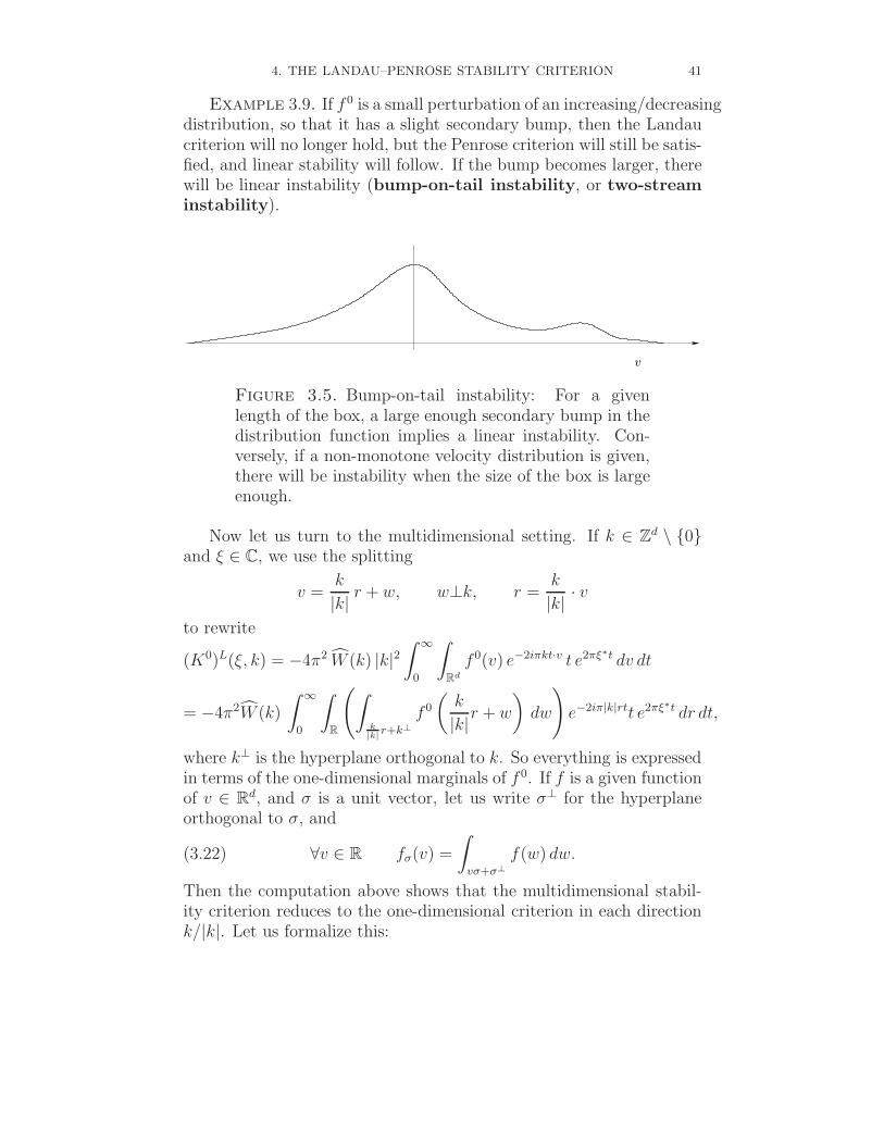
Example 3.9. If f 0 is a small perturbation of an increasing/decreasingdistribution, so that it has a slight secondary bump, then the Landaucriterion will no longer hold, but the Penrose criterion will still be satis-fied, and linear stability will follow. If the bump becomes larger, therewill be linear instability (bump-on-tail instability, or two-stream

instability).

v

Figure 3.5. Bump-on-tail instability: For a givenlength of the box, a large enough secondary bump in thedistribution function implies a linear instability. Con-versely, if a non-monotone velocity distribution is given,there will be instability when the size of the box is largeenough.

Now let us turn to the multidimensional setting. If k ∈ Zd \ 0and ξ ∈ C, we use the splitting

v =k

|k| r + w, w⊥k, r =k

|k| · v

to rewrite

(K0)L(ξ, k) = −4π2 W (k) |k|2∫ ∞

0

∫

Rd

f 0(v) e−2iπkt·v t e2πξ∗t dv dt

= −4π2W (k)

∫ ∞

0

∫

R

(∫

k|k|

r+k⊥

f 0

(k

|k|r + w

)dw

)e−2iπ|k|rtt e2πξ∗t dr dt,

where k⊥ is the hyperplane orthogonal to k. So everything is expressedin terms of the one-dimensional marginals of f 0. If f is a given functionof v ∈ Rd, and σ is a unit vector, let us write σ⊥ for the hyperplaneorthogonal to σ, and

(3.22) ∀v ∈ R fσ(v) =

∫

vσ+σ⊥

f(w) dw.

Then the computation above shows that the multidimensional stabil-ity criterion reduces to the one-dimensional criterion in each directionk/|k|. Let us formalize this:


Definition 3.10 (Penrose’s stability criterion). We say that f 0 =f 0(v) satisfies the (generalized) Penrose stability criterion for the in-teraction potential W if for any k ∈ Zd, and any ω ∈ R,

(f 0σ)′(ω) = 0 =⇒ W (k)

∫(f 0

σ)′(v)

v − ωdv < 1, σ =

k

|k| .

Example 3.11. The multidimensional generalization of Landau’sstability criterion is that all marginals of f 0 are increasing/decreasing.

Example 3.12. If f 0 is radially symmetric and positive, and d ≥ 3,then all marginals of f 0 are decreasing functions of |v|. Indeed, if

ϕ(v) =∫

Rd−1 f(√v2 + |w|2) dw, then after differentiation and integra-

tion by parts we findϕ′(v) = −(d − 3) v

∫

Rd−1

f(√

v2 + |w|2) dw|w|2 (d ≥ 4)

ϕ′(v) = −2π v f(|v|) (d = 3).

5. Asymptotic behavior of the kinetic distribution

Let us assume stability, so that the force F [h] converges to 0 ast → ∞, exponentially fast in an analytic setting. What happens to hitself?

Starting again from

(3.23) h(t, k, η) = hi(k, η + kt)

− 4π2 W (k)

∫ t

0

ρ1(τ, k) f 0(η + k(t− τ)) k ·[η + k(t− τ)

](t− τ) dτ

we can control the integrand on the right-hand side by the bounds

|ρ(τ, k)| = O(e−2πλ′|k|τ), |f 0(η)| = O(e−2πλ′|η+k(t−τ)|).

Sacrificing a little bit of the τ -decay of |ρ| to ensure the convergenceof the τ -integral, using |η + kt| ≤ |η + k(t − τ)| + |kτ |, and assuming

|k|W (k) = O(1) (which is true if ∇W ∈ L1), we end up with∣∣∣∣4π2 W (k)

∫ t

0

ρ1(τ, k) f 0(η + k(t− τ)) |k|2 (t− τ) dτ

∣∣∣∣ = O(e−2πλ′′|η+kt|

),

where λ′′ is arbitrarily close to λ′. Plugging this back in (3.23) implies

(3.24)∣∣h(t, k, η) − hi(k, η + kt)

∣∣ ≤ C e−2πλ′′|η+kt|.

It is not difficult to show that the bound (3.24) is qualitatively optimal;

it is interesting only for k 6= 0, since we already know h(t, 0, η) =

hi(0, η).

6. QUALITATIVE RECAP 43

Let us analyze (3.24) as time becomes large. First, for each fixed

(k, η) we have h(t, k, η) −→ 0 exponentially fast, in particular

h(t, ·) t→∞−−−→weakly

〈hi〉,

and the speed of convergence is determined by the regularity in velocityspace: exponential convergence for analytic data, inverse polynomialfor Sobolev data, etc.

However, for each t one can find (k, η) such that |h(t, k, η)| is O(1)(not small!). In other words, the decay of Fourier modes is not uniform,and the convergence is not strong. In fact, the spatial mode k ofh(t, · ) undergoes oscillations along the kinetic frequency η ≃ −kt inthe velocity variable as t→ ∞; so at time t, the typical oscillation scalein the velocity variable is O(1/|k|t) for the mode k. How much large|k| modes affect the whole distribution h depends on the respectivestrength of the modes, that is, on the regularity in the x variable; but inany case the kinetic distribution h will exhibit fast velocity oscillationsat scales O(1/t) as t goes by. The problem only arises in the velocityvariable: it is an easy exercice to check that the smoothness in theposition variable is essentially preserved.

However, if one considers h along trajectories of free transport, the

smoothness is restored: (3.24) shows that h(t, k, η−kt) is bounded likeO(e−2πλ′′|η|), so we do not see oscillations in the velocity variable anylonger. Let us call this the gliding regularity: if we change the focusin time to concentrate on modes η ≃ −kt in Fourier space, we do seea good decay. Equivalently, if we look at h(x + vt, v), what we see isuniformly smooth as t→ ∞.

This point of view can also be given an appealing interpretation as afinite-time scattering procedure. As t→ ∞, the force field vanishes,so the linearized Vlasov equation is asymptotic to the free transportevolution. Now the idea is to let the distribution evolve according to thelinearized Vlasov for time t, then apply the free evolution backwardsfrom time t to initial time, and study the result. This is the same asone does in classical scattering theory, except that in scattering theoryone would take the limit t→ ∞, and we prefer to have estimates thatare uniform in time, not just in the limit.

6. Qualitative recap

Let me reformulate and summarize what we learnt in this section.I shall start with a precise mathematical statement.


Theorem 3.13. Let f 0 = f 0(v) be an analytic homogeneous equilib-

rium, with |f 0(η)| = O(e−2πλ0|η|), and let W be an interaction potentialsuch that ∇W ∈ L1(Td). Let K0 be defined in (3.14); assume that thereis λL > 0 such that the Laplace transform (K0)L(ξ, k) of K0(t, k) staysaway from the value 1 when 0 ≤ Re ξ < λL|k|. Let hi = hi(x, v) be an

analytic initial perturbation such that hi(k, η) = O(e−2πλ|η|). Then ifh solves the linearized Vlasov equation (3.6) with initial datum hi, onehas exponential decay of the force field: for any k 6= 0,

F [h](t, k) = O(e−2πλ′|k|t),

for any λ′ < min(λ0, λL, λ). Moreover, Penrose’s stability condition(Definition 3.10) guarantees the existence of λL > 0.

Remark 3.14. Following Landau, physics textbooks usually careonly on λL and forget about λ0, λ, assuming that f 0 and hi are entirefunctions (so one can choose λ0 and λL arbitrarily large). But in gen-eral one should not forget that the damping rate does depend on theanalytic regularity of f 0 and hi.

Beyond Theorem 3.13, one can argue that the three key ingredientsleading to the decay of the force field are

• the confinement ensured by the torus;• the mixing property of the geodesic flow (x, v) → (x+ vt, v);• the Riemann–Lebesgue principle converting smoothness into de-

cay in Fourier space.

The first two ingredients are important: as I already mentioned,there are counterexamples showing that decay does not hold in thewhole space, and it is rather well-known from experiments that damp-ing may cease when the flow ceases to be mixing, so that for instancetrapped trajectories appear. As for the third ingredient, it is subject todebate, since there are many points of view around as to why dampingholds (wave-particle interaction, etc.), but in these notes I will advocatethe Riemann–Lebesgue point of view as natural and robust.

Now as far as the regularity of h is concerned, one should keep inmind that

• the regularity of h deteriorates in the velocity variable, as itoscillates faster and faster in v as time increases;

• there is a cascade in Fourier space from low to high kinetic modes,which on the mean is faster for higher position modes — it is like ashear flow in Fourier space;


• the distribution function evaluated along trajectories of the freeflow, h(t, x + vt, v), remains very smooth, uniformly in time (glidingregularity).

While the regularity of h deteriorates in the kinetic variable, on thecontrary, the regularity of the force field increases with time, since (inanalytic regularity)

(3.25) F (t, 0) = 0, |F (t, k)| = O(e−2πλ|k|t).

Of course this implies the time decay of F like O(e−2πλt), but (3.25) ismuch more precise by keeping track of the respective size of the variousmodes. A simplistic way to summarize these apparently conflicting be-haviors is that there is deterioration of the regularity in v, improvementof the regularity in x.

In the study of the linearized equation, we can live without knowingall this qualitative information, and it is not surprising that it hasapparently never been recorded in a fully explicit way. But this willbecome crucial in our analysis of the nonlinear equation.


Landau [56] solved the linearized Landau equation by using theseparation of modes and the Fourier–Laplace transform. His treatment,based on the inversion of the Laplace transform, has been reproducedin countably many sources [1, 8, 14, 29, 43, 54, 61, 69, 89]. Therigorous justification is somewhat tricky because inverting a Laplacetransform is not such a simple matter and involves integration overa complex contour, which has to be chosen properly; in fact Vlasovhad it wrong in this respect, and Landau was the first to identify thissubtlety. The first completely rigorous treatment is due to Backus[8]. Morrison [71] formalized the complete integrability property ofthe system, thanks to the so-called R-transform, which is related tothe Laplace inversion.

An alternative solution consists in expressing the solution as a com-bination of generalized eigenfunctions, called Van Kampen modes

[22, 61, 98]. This reduces the stability analysis to the study of adispersion equation, but this is even more complicated to justify.

The presentation adopted in this chapter, taken from [74], is muchmore elementary since it replaces the tricky Laplace inversion formulaby the standard Fourier inversion formula. This simple but downrightunorthodox treatment was suggested by a conversation with Sigal. Theprice to pay (but we don’t really care) for this simple approach is thatinstead of having an exact representation of the solution, we just have


an estimate on it. On the other hand, a considerable reward is thatthis estimate easily goes through the nonlinear study.

Counterexamples by Glassey and Scheffer, showing that there is noLandau damping in the whole space for the linearized Vlasov–Poissonequation, can be found in [36, 37]. Estimates of the decay rate at smallwavelengths (large distances) are performed in [56] or [61, Section 32].

In 1960 Penrose [82] suggested that the violation of the criterion(3.21) would lead to instability. In particular, he argued that if thedistribution function has a secondary bump (is nonmonotone) then thedistribution is linearly unstable at large enough scales. Conversely, thePenrose criterion implies stability under small-scale perturbations. Linand Zeng [59] have shown that the Penrose criterion is close to be anecessary and sufficient condition. Example 3.12 is taken from [61,Problem, Section 30] (in dimension d = 3).

The interpretation of the Jeans instability can be found in [14]; itdoes not work quantitatively so well to predict the typical galaxy diam-eter, because galaxies are not really a continuum of stars. In a phasediagram for galaxies, the Jeans length is a “spinodal” (metastability)point, which only gives an upper bound for the phase transition regime[93].

The scattering approach to Landau damping was considered byCaglioti and Maffei [21], and amplified in my work with Mouhot [74].A self-contained treatment of the linearized Vlasov–Poisson equationcan be found in Section 3 of the latter work.

Ryutov [88] mentions that interpretations of the Landau dampingphenomenon were still regularly appearing fifty years after the discov-ery of this effect. The wave-particle interpretation is surveyed, some-times critically, in the works of Elkens and Escande [32, 33, 34]

Belmont [11] noticed that the damping rate in the linearized equa-tion depends not only on the Landau stability condition, but also onthe regularity of f 0, so that “for special distribution functions” theLandau damping rate does not govern the damping of the force.

CHAPTER 4

Nonlinear Landau damping

The damping phenomenon discovered by Landau, and consideredin the previous chapter, is based on the study of the linearized Vlasovequation. But the physical model, of course, is the nonlinear equation,so the question naturally arises whether damping still holds for thatmodel, at least in the perturbative regime, that is, near a spatiallyhomogeneous equilibrium.

1. Nonlinear stability?

Linear stability is often a necessary condition for nonlinear stability,but is it sufficient? Starting from the nonlinear Vlasov equation, wehave implicitly considered two distinct asymptotic regimes: t → ∞and ε → 0, where ε = ‖fi − f 0‖; and these two limits a priori do notcommute! In large time, small cumulated nonlinear effects might leadto a significant departure from the linearized equation.

To estimate the time scale on which this may occur, let us look fora scale invariance of the Vlasov equation. Let us assume that f = 1+hsolves the Vlasov equation (forget the fact that f has infinite mass),and set

fε(t, x, v) = 1 + ε1+dν h(εθt, x, ενv

),

where ν and θ are unknown parameters. (We cannot rescale in x sincewe work with periodic boundary conditions.) Note that fε−1 is of sizeε in L1 norm, and

∫(fε − 1) dv = O(ε). Then

∂tfε + v · ∇xfε + F [fε] · ∇vfε

= ε1+dν[εθ ∂th + ε−ν (v · ∇xh) + ε1+ν (F · ∇vh)

](εθ t, x, εν v),

so fε solves the Vlasov equation if θ = −ν = 1 + ν, i.e. θ = 1/2 = −ν.In other words,

(4.1) fε(t, x, v) = 1 + ε1− d2 h

(√ε t, x,

v√ε

)

also solves the Vlasov equation. This suggests the typical nonlineartime scale O(1/

√ε), where ε is the size of the perturbation. This is

47

48 4. NONLINEAR LANDAU DAMPING

the O’Neil time scale and it is indeed well satisfied in numericalexperiments.

To summarize: after a time scale O(1/√ε) we expect the solution of

the nonlinear Vlasov equation to be significantly different from the so-lution of the linearized approximation; in particular, it is not clear thatthe large-time limit of the linearization coincides with the linearizationof the large-time limit.

The problem arises not only for the study of the damping, but alsoalready for the a priori simpler stability problem: for many years it hasbeen an open problem to show that Penrose’s linear stability conditionguarantees nonlinear stability. Only the simpler stability condition byLandau (monotone profile) could be treated by Lyapunov functionaltechniques.

2. Elusive bounds

The study of the linearized Vlasov equation ∂th + v · ∇xh + F [h] ·∇vf

0 = 0 showed that the expected decay rate depends (among otherthings) on the smoothness of f 0. In the nonlinear case we have ∂tf +v · ∇xf + F [f ] · ∇vf = 0, so the uniformly smooth background f 0(v)is replaced by the time-dependent distribution f(t, x, v), which maybe analytic, but not uniformly in time: fast oscillations in the velocityvariable, a phenomenon which is also known as filamentation in phasespace, will imply the blow-up of all regularity bounds of f in large time.Then how can one hope to adapt the tools on which the linearized studywas based??

3. Backus’s objection

When one linearizes the Vlasov equation as in the beginning of theprevious chapter, one neglects the quadratic term F [h] · ∇vh in frontof the others, assuming implicitly that ‖h‖ is much smaller than ‖f 0‖in some sense. However, ∇vh cannot stay small in the usual sense: itsnorm will typically grow in time — unless we use a weak norm, but weare in a context where smoothness matters much. To see this growth,let us consider just the simpler free transport: if ∂th + v · ∇xh = 0,then

∇vh(t, k, η) = 2iπη h(t, k, η) = 2iπη hi(k, η + kt).

Then even if hi is of size ε≪ 1, the choice η ≃ −kt shows that

supη

∣∣∣∇vh(t, k, η)∣∣∣ ≥ const. ε|k|t

5. THEOREM 49

as t → +∞, so ‖∇vh‖L1(dx dv) grows at least linearly in time. As aconsequence, if we wait long enough, there will necessarily come a timewhen the linearization postulate is no longer satisfied! This objectionwas raised by Backus in 1960.

Of course, F [h] ·∇vh might still decay in time, since we expect F [h]to decay exponentially fast, and ∇vh to grow at most linearly. Butright now we cannot understand why the effect of this term would benegligible compared to the effect of other terms like F [h] ·∇vf

0, whichwe also expect to be decaying exponentially fast!

4. Numerical simulations

Numerical simulations about the large-time behavior of the non-linear Vlasov–Poisson equation are nonconclusive because of the diffi-culties in getting reliable simulations on very large times. If ε is thesize of the perturbation, nonlinear effects start to appear at time scaleO(1/

√ε), and then tiny numerical errors cumulated over very large

times can be dreadful.To summarize the situation, one can say that

• for a slight perturbation of the equilibrium, numerical schemesdo display the Landau damping phenomenon for large times, and someof them continue to display damping at very large times, while otherones present tiny bumps of the electric field, which sometimes do notvanish as t→ ∞;

• for a larger perturbation of the equilibrium, numerical schemesagree that damping may be replaced by a much more complicatedbehavior, leading to a persistent electric field. Some authors claimto observe BGK waves in very large times, while others remain morecautious.

Francis Filbet kindly accepted to do a few precise simulations for mein the perturbative regime, with different methods; they led to differentresults, but the one that was supposed to be the most precise displayeddamping at spectacular precision (more than 20 orders of magnitudefor the amplitude of the electric field, and at times so large that thenonlinear effects can definitely not be neglected; see Figures 4.1 and4.2).

5. Theorem

Some of the previous questions are solved by the following theoremby Mouhot and myself. If n is a multi-integer and f a function I shallwrite f (n) = ∇nf = ∂n1

1 . . . ∂ndd f .


-28

-26

-24

-22

-20

-18

-16

-14

-12

-10

-8

-6

0 5 10 15 20 25 30 35 40

log(

|| E

(.)

||)

t

d = 0.001d = 0.002d = 0.004d = 0.006d = 0.008d = 0.010

-35

-30

-25

-20

-15

-10

-5

0 5 10 15 20 25 30 35 40

log(

|| E

(.)

||)

t

d = 0.001d = 0.002d = 0.004d = 0.006d = 0.008d = 0.010d = 0.012

Figure 4.1. Large time behavior of the logarithm ofthe norm of the electric field, with two different numer-ical methods — the second one is supposed to be moreprecise. The interaction is gravitational, the initial da-tum is a Gaussian multiplied by 1 + ε cos(2πkx).

-0.1

0

0.1

0.2

0.3

0.4

0.5

0.6

0.7

0.8

0.9

0 5 10 15 20 25 30 35 40

log(

|| E

(.)

||) -

log(

|| E

l(.)

||)

t

d = 0.001d = 0.002d = 0.004d = 0.006d = 0.008d = 0.010d = 0.012

-0.1

0

0.1

0.2

0.3

0.4

0.5

0.6

0.7

0.8

0.9

0 0.5 1 1.5 2 2.5 3 3.5 4

log(

|| E

(.)

||) -

log(

|| E

l(.)

||)

d^1/2 t

d = 0.001d = 0.002d = 0.004d = 0.006d = 0.008d = 0.010d = 0.012

Figure 4.2. With the more precise method from Figure4.1, a plot of log(‖ENL‖/‖EL‖), the logarithmic ratio ofthe norm of the nonlinear electric field to the norm ofthe linearized electric field. On the left the time-scale is1, on the right the time scale is 1/

√ε. Here we see that

we arrive in a time regime where the nonlinearity candefinitely not be neglected.

Theorem 4.1. Let f 0 = f 0(v) be an analytic profile satisfying thePenrose linear stability condition. Further assume that the interactionpotential W satisfies

(4.2) W (k) = O

(1

|k|2).

5. THEOREM 51

Then one has nonlinear stability and nonlinear damping close to f 0.More precisely, assume that (a) f 0 is analytic in a strip of width

λ0 > 0, in the sense that

|f 0(η)| ≤ C0 e−2πλ0|η|,

∑

n∈Nd

λn0

n!‖∇n

vf0‖L1(dv) ≤ C0;

(b) the Penrose linear stability condition is satisfied in a strip of width

λL, in the sense that, if K0(t, k) = −4π2 W (k) f 0(kt) |k|2t, then

(4.3) 0 ≤ Re ξ ≤ λL|k| =⇒ |(K0)L − 1| ≥ κ > 0.

(c) the initial condition fi is a perturbation of f 0 in a strip of widthλ > 0, in the sense that

|fi−f0|(k, η) ≤ ε e−2πµ|k| e−2πλ|η|,

∫|fi(x, v)−f 0(v)| e2πβ|v| dx dv ≤ ε

for some µ > 0, β > 0. Then if ε ≤ ε∗ = ε∗(λ0, λL, λ, µ, κ, C0, β),for any λ′ < min(λ0, λL, λ), if f(t, · ) is the solution of the nonlinearVlasov equation with interaction W and initial datum fi, and F = F [f ]is the associated force field, one has

‖F (t, · )‖ = O(ε e−2πλ′t) as t→ +∞;

also ρ(t, x) converges (strongly and exponentially fast) to the averageρ∞ =

∫∫fi(x, v) dx dv.

Moreover,

f(t, · ) t→±∞−−−−→weakly

f±∞,

where f±∞ = f±∞(v) is an analytic homogeneous equilibrium; and

〈f(t, · )〉 t→±∞−−−−→strongly

f±∞,

where 〈 · 〉 stands for the x-average.

Remarks 4.2. Here is a long series of remarks:

1. The condition W (k) = O(1/|k|2) seems critical, and only appearsin the study of the nonlinear problem. It would somehow be easier tohandle a decrease like O(1/|k|2+δ); this may be a coincidence or somedeep thing.

2. The analytic norm used for fi − f 0 is the most naive normcontrolling exponential localization in Fourier space and in physicalspace. Also the smallness restriction on the size of ε is natural.

3. The decay of the force field is the damping phenomenon; theexistence of limit distributions f+∞ and f−∞ is a bonus. These distri-butions are not determined by variational principles (at least, not that


I know) and may differ for t→ +∞ and t→ −∞. When f+∞ 6= f−∞,such trajectories may be called heteroclinic, as opposed to homoclinictrajectories for which the behavior for t → +∞ is the same as fort→ −∞ (as in the case of the linearized Vlasov equation). It is strik-ing to see that a whole neighborhood of f 0 (stable equilibrium) is filledby homoclinic/heteroclinic trajectories. This is not predicted by the(random) quasilinear theory of the Vlasov–Poisson equation, neitherby the statistical theory: there is in fact no randomness in Theorem4.1. This abundance of homoclinic/heteroclinic orbits is possible onlybecause, thanks to the infinite dimension, one can play with the varioustopologies. The fact that the conditions for damping are expressed interms of the initial condition alone is a considerable improvement overprevious works in the field.

4. The proof provides a constructive approach of the long-timebehavior of f , which makes it possible to exchange the limits ε → 0and t → ∞, perform asymptotic expansions, etc. In particular, onecan check that the asymptotic state f+∞ “keeps the memory” of theinitial datum, in a way that goes beyond the invariants of motion. Themere existence of heteroclinic trajectories demonstrates this: reversingtime does not change the energy neither any of the constants of motionwhich were mentioned in Chapter 2, but will change the asymptoticbehavior. This seems to confirm an objection raised by Isichenko in1966 against the statistical theory of the nonlinear Vlasov equation.However, on second thoughts, the statistical theory can counterattack,because of the high regularity which is involved in the result. Theorem4.1 is based on an analytic regularity; even if this is later relaxed ina Sobolev or even Cr regularity, these classes of regularity are prob-ably negligible in a statistical context, where typical distributions areprobably not smooth. (For instance, typical distributions for Sturm’sentropic measure are not even absolutely continuous!)

5. The theorem in this section provides a perturbative large-timeexistence result which is covered neither by the Lions–Perthame theory(because this is a periodic setting) nor by the Pfaffelmoser–Batt–Reintheory (because the analyticity assumption is not compatible with acompact support).

6. An important corollary of the theorem is the orbital stability ina strong sense: if Hs

x,v stands for the L2-Sobolev space of order s on

Tdx ×Rd

v, then under the assumptions of Theorem 4.1, for any s > 0 wehave

(4.4)∥∥∥f(t, x+ vt, v) − f 0(v)

∥∥∥Hs

x,v

= O(ε),

6. THE INFORMATION CASCADE 53

uniformly as t→ +∞. Since L2(dx dv) is invariant under the action offree transport, the norms in (4.4) control ‖f(t, ·)− f 0‖L2(Rd×Td). Usingmoment bounds and Sobolev injections, one may also control f − f 0 inLp norms, for all p ≥ 1.

7. The critical regularity to which the proof applies is the Gevreyclass Gν , for any ν < 3 in the favorable cases. By convention, a func-tion f belongs to the Gevrey class Gν if f (n) = O(n!ν), say in thesupremum norm. Modulo an arbitrarily small loss on the exponent ν,

it is equivalent to say that the Fourier transform f(ξ) of f decays at

infinity like O(e−c|ξ|1/ν). The favorable case alluded to above is the one

in which∫|K(t, k)| dt < 1; this applies for instance for gravitational

interaction below the Jeans length. More generally, if the interaction

satisfies |W (k)| = O(1/|k|1+γ) and∫|K(t, k)| dt < 1 then the critical

exponent is ν = γ + 2. Here is a precise statement where we do notcare about the critical exponent:

Theorem 4.3 (Nonlinear Landau damping in Gevrey regularity).

Let W : Td → R be an interaction potential such that |W (k)| =O(1/|k|2). Let f 0 = f 0(v) be an analytic profile such that

|f 0(η)| ≤ C0 e−2πλ0|η|,

∑

n

λn0

n!‖∇n

vf0‖L1(dv) ≤ C0,

for some λ0 > 0, and satisfying the Penrose stability condition withLandau width λL > 0. Then there is θ > 0 such that for any ν ∈(1, 1 + θ), β > 0, α < 1/ν, there is ε∗ > 0 such that if

ε := supk,η

(∣∣(fi−f 0)(k, η)∣∣ eλ|η|1/ν

eλ|k|1/ν)+

∫∫|fi(x, v)−f 0(v)| eβ|v| dv dx

satisfies ε ≤ ε∗, then the solution f = f(t, x, v) of the nonlinear Vlasovequation with interaction W and initial datum fi satisfies

F [f ](t, · ) = O(ε e−ctα

),

and f(t, · ) converges weakly to some asymptotic Gevrey profile f±∞ =f±∞(v) as t→ ±∞, with convergence rate O(ε e−ctα).

6. The information cascade

How can one reconciliate the reversibility of the nonlinear Vlasovequation and the convergence in large time? Convergence seems to beabout loss of information, which should go with an increase of entropy;but we have seen that the Vlasov equation preserves the entropy. Sowhat?


The solution to this apparent paradox (well understood by somephysicists at least fifty years ago, but not by all of them) is that theinformation all goes out to high frequencies, where it is inaccessible,hidden. The following numerical simulations will illustrate this.

-4e-05

-3e-05

-2e-05

-1e-05

0

1e-05

2e-05

3e-05

4e-05

-6 -4 -2 0 2 4 6

h(v)

v

t = 0.16

-4e-05

-3e-05

-2e-05

-1e-05

0

1e-05

2e-05

3e-05

4e-05

-6 -4 -2 0 2 4 6

h(v)

v

t = 2.00

Figure 4.3. A slice of the distribution function (relativeto a homogeneous equilibrium) for gravitational Landaudamping, at two different times; notice the fast oscilla-tions of the distribution function, which are very difficultto capture by an experiment.

-13

-12

-11

-10

-9

-8

-7

-6

-5

-4

0 10 20 30 40 50 60 70 80 90 100

log(

Et(

t))

t

electric energy in log scale

-23

-22

-21

-20

-19

-18

-17

-16

-15

-14

-13

-12

0 0.05 0.1 0.15 0.2 0.25 0.3 0.35 0.4

log(

Et(

t))

t

gravitational energy in log scale

Figure 4.4. Time-evolution of the norm of the field, forelectrostatic (on the left) and gravitational (on the right)interactions. In the electrostatic case, the fast time-oscillations are called Langmuir oscillations, and shouldnot be mistaken with the velocity oscillations.

In fact, the cascade of energy, already present in the free transportevolution, still holds: energy (or information) flows from low to highfrequencies. The complete integrability has been lost, but the energy


transfer still holds. This is similar in spirit to the KAM phenomenon

(KAM = Kolmogorov–Arnold–Moser), to which we shall come backlater; for the moment I will just mention that there are common pointsand differences with the KAM theory.

To go back to the information, let us note that∫∫

f log f =

∫ρ log ρ+

∫∫f log

f

ρ,

and the first term on the right-hand side converges to 0 because ρ con-verges strongly to a constant. So all the information becomes “kinetic”in the limit. (Due to the oscillations, a priori we cannot pass to thelimit; but that becomes possible if we go along trajectories of the freetransport and use the gliding regularity.)

A final remark is in order: because of the time-reversibility, anystability result, read backwards in time, should imply an instabilityresult. This is true, however with a catch on the topologies involved.Landau damping asserts convergence in large time in the weak topol-ogy, when the initial datum is perturbed in the strong topology. Read-ing it backwards implies a instability in the strong topology, when theinitial datum is perturbed in the weak topology. In particular, Landaudamping is by no means in contradiction with the time-reversibility.


Backus [8] was certainly the first one to point out the conceptualproblem caused by the interversion of the asymptotic regimes t → ∞and ‖fi − f 0‖ → 0. Thus his paper contains both positive state-ments (the first mathematically rigorous treatment of the linear Landaudamping) and expression of skepticism, which has not been answereduntil [74].

Nonlinear stability of monotone homogeneous profiles for the elec-trostatic Vlasov–Poisson equation was studied by Rein [86]. The two-stream instability has been established by Guo and Strauss [41].

The nonlinear time scale O(1/√ε) was predicted in 1965 by O’Neil

[81] with a more sophisticated argument than the naive scaling ap-proach presented in Section 1, and is anyway well checked in numericalsimulations. This is the time scale where significant departure appearsbetween the solutions of the linear and nonlinear equations; it does notmean that the qualitative behavior of these solutions differ much. Ac-tually, O’Neil argues that damping still holds true for larger time scales,even though not infinite. He also stumbles on the problem pointed outby Backus.


Numerical investigation of the Landau damping, for small and largerperturbations, was performed by several authors at the end of thenineties, when precise methods started to be available [67, 105]. Sincethen, more efficient schemes have become available [44].

The mysterious but popular quasilinear theory is presented in anumber of sources [61, Section 49] [1, Section 9.1.2] [54, Chapter 10],with more or less convincing arguments. Putting this theory on adecent level of rigor looks like a challenge.

Isichenko’s criticism of the statistical theory of Vlasov equation ap-pears in [51]. Using an analogy with a random potential problem, heargues that the convergence to equilibrium should be slow; howeverthe analogy used by Isichenko is not so sound, and in fact very fastconvergence can occur, as demonstrated in [21] and in the present pa-per. Isichenko’s paper is still worth reading for his interesting insights,though.

Theorem 4.1 is taken from [74], as well as the comments made rightafter its statement.

Caglioti and Maffei [21] were the first to construct some exponen-tially damped solutions to the Vlasov–Poisson equation (in dimen-sion 1); they also noted that this implies, by time-reversibility, theinstability in the weak topology. Another construction to damped so-lutions was performed by Hwang and Velazquez [50].

The numerical simulations in this chapter were kindly provided byFilbet.

CHAPTER 5

Gliding analytic regularity

Analytic regularity may seem very specific, but it is for sure thefirst setting to understand in the study of Landau damping, for phys-ical reasons (because it is associated to exponential damping) and forhistorical reasons as well (because this is the case that was treated byLandau). But the obstacles related to the study of the limit t → ∞require much care in the choice of functional space.

1. Preliminary analysis

There are many families of analytic norms. A particularly simplefamily is defined by the formula

(5.1) ‖f‖λ,µ = supk,η

∣∣f(k, η)∣∣ e2πµ|k| e2πλ|η|.

One can interpret λ and µ as the width of the analyticity strip in thev and x variables, respectively.

To evaluate the relevance of these functional spaces, let us examinethe equation and seek to approximate it by an iterative scheme. Thenatural quasilinear scheme is

(5.2) ∂tfn+1 + v · ∇xf

n+1 + F [fn] · ∇vfn+1 = 0,

which amounts to let particles evolve at stage n + 1 in the force fieldcreated by the distribution at stage n. Equivalently, one solves thetransport equation by the characteristic method:

fn+1(t, x, v) = fi

(Sn

t,0(x, v)),

where Snt,0(x, v) is the position (in phase space) at time 0 of particles

evolving in the force field induced by fn, which at time t will be at(x, v). Thus one is naturally led to study the behavior of norms withrespect to composition. But these norms do behave very badly: to fixideas, let us assume that St(x, v) satisfies “perfect” estimates, as good

57

58 5. GLIDING ANALYTIC REGULARITY

as (say) 2 Id ; and observe that

∥∥f (2 Id )∥∥

λ,µ= 2d sup

k,η

∣∣∣∣f(k

2,η

2

)∣∣∣∣ e2πµ|k| e2πλ|η|

= 2d supk,η

∣∣f(k, η)∣∣ e2π(2µ)|k| e2π(2λ)|η|

= 2d ‖f‖2λ,2µ.

In other words, the norms λ, µ are not stable under composition. This isin sharp contrast with Sobolev or Cr norms. Now imagine the disaster:as one iterates the estimates, one loses a factor 2 on the width of theanalyticity strip, so that there is nothing left in the end...

What is more, (5.2) will not express a reaction: recall the heuristicimage about pushing the wall and exhausting oneself. It would be morepromising to use the alternative scheme

∂tfn+1 + v · ∇xf

n+1 + F [fn+1] · ∇vfn = 0.

But this would mean treating a higher order degree, ∇vfn, as a per-

turbation: thus there would be a loss of derivative.A third problem is related to the filamentation: the best one can

hope for f is estimates in the style of the solution of free transportg(k, η + kt); so in the best of worlds,

∣∣f(t, k, η)∣∣ ≤ C e−2πλ|η+kt| e−2πµ|k|.

But then ‖f‖λ,µ & e2πλt (choose η = −kt, |k| = 1); and even worse,‖f‖λ,µ & e2πλ|k|t for any k such that the mode k does not vanish. Ifall modes k are represented, one expects the norm of f to grow fasterthan any exponential! This of course is a disaster for the large-timeanalysis.

2. Algebra norms

Among all families of analytic norms, two deserve a special mention;let us present them in dimension 1:

(5.3) ‖f‖Fλ =∑

k∈Z

e2πλ|k| |f(k)| ‖f‖Cλ =∑

n∈N0

λn

n!‖f (n)‖L∞,

where f (n) stands for the derivative of order n of f , and N0 = 0, 1, 2, . . ..The first norm (as it is written) makes sense only for periodic functions,while the second one makes sense for any smooth function on R.

Proposition 5.1. With ‖ · ‖λ standing either for the Fλ or the Cλ

norm, one has‖fg‖λ ≤ ‖f‖λ ‖g‖λ.

2. ALGEBRA NORMS 59

Sketch of proof. Let us prove the inequality for, say, the Cλ

norm: the Leibniz differentiation formula implies

∑

n

λn

n!

∥∥(fg)(n)∥∥

L∞ ≤∑

n

∑

m≤n

λn

n!

n!

m! (n−m)!‖f (m)‖L∞ ‖g(n−m)‖L∞

=∑

m,m′

λm+m′

m!m′!‖f (m)‖L∞ ‖g(m′)‖L∞

=

(∑

m

λm

m!‖f (m)‖L∞

) (∑

m′

λm′

m′!‖f (m′)‖L∞

).

As an immediate corollary, we have ‖fn‖λ ≤ ‖f‖nλ. This remarkable

algebra property implies good properties with respect to compositionas well: there will be a loss of exponent, that is unavoidable, but it willbe controlled.

Proposition 5.2. With ‖ · ‖λ standing either for the Fλ or the Cλ

norm, one has

∥∥∥f (Id +G)∥∥∥

λ≤ ‖f‖ν , ν = λ+ ‖G‖λ.

Note carefully: the constant in front of the right-hand side is equalto 1; and the size of G (in the λ-norm) is found in the regularity indexon the right-hand side.

Sketch of proof of Proposition 5.2. Let us do it for the Cλ

norm. Writing h = f (Id +G) and using the Taylor formula (leavingaside the issue of convergence), we have

h(x) =∑

n

f (n)(x)

n!Gn(x),

whence

h(m)(x) =∑

k+ℓ=m

∑

n

m!

k! ℓ!n!f (n+k)(x) (Gn)(ℓ)(x),


so∑

m

λm

m!‖h(m)‖L∞ ≤

∑

m

∑

k+ℓ=m

∑

n

λk+ℓ

k! ℓ!n!‖f (n+k)‖L∞ ‖(Gn)(ℓ)‖L∞

=∑

k,ℓ,n

λk+ℓ

k! ℓ!n!‖f (n+k)‖L∞ ‖(Gn)(ℓ)‖L∞

≤∑

k,n

λk

k!n!‖Gn‖λ ‖f (n+k)‖L∞

≤∑

r

( ∑

k+n=r

r!

k!n!λk ‖G‖n

λ

)‖f (r)‖L∞

r!

≤∑

r

(λ+ ‖G‖λ

)r

r!‖f (r)‖L∞

= ‖f‖λ+‖G‖λ,

where Newton’s binomial formula was used.

Proposition 5.2 admits some variants: in particular, it is possibleto mix norms:

(5.4)∥∥∥f (Id +G)

∥∥∥Cλ

≤ ‖f‖Fν , ν = λ+ ‖G‖Cλ,

where the Cλ seminorm is obtained from the Cλ norm by throwing awaythe zero mode. (The proof of (5.4) involves the dreaded Faa di Brunoformula.)

Working in kinetic theory, it is particularly convenient to hybridizethe two spaces: apply the recipe C to the velocity space, and the recipeF to the position space. This will take advantage of the periodic ge-ometry of the position space, and property (5.4) will guarantee thatcomposition by the characteristics is still properly handled. Let us alsogeneralize to d dimensions, add a parameter γ to count derivatives (fortechnical reasons, this is needed only in the x variable), and anotherparameter p to modulate the integrability; we are led to the formula

(5.5) ‖f‖Zλ,(µ,γ);p =∑

k∈Zd

∑

n∈Nd0

e2πµ|k| (1 + |k|)γ λn

n!

∥∥∇nv f(k, v)

∥∥Lp(dv)

,

where f(k, v) =∫f(x, v) e−2iπk·x dx is the Fourier transform of f in the

x variable only. Then we have good properties generalizing Property5.1 such as

‖fg‖Zλ,(µ,γ);p ≤ ‖f‖Zλ,(µ,γ);q ‖g‖Zλ,(µ,γ);r ,1

r=

1

p+

1

q.

3. GLIDING REGULARITY 61

3. Gliding regularity

Now it remains to take into account filamentation, that is, the ap-pearance of fast oscillations in the velocity variable. Since we cannotavoid it, let us accept it and incorporate it in the norm. This amountsto introducing a parameter τ (time-like) and to let the free transportevolution act backwards on the distribution function, for a time τ :

‖f‖Zτ = ‖f S0−τ‖Z ,

where the regularity indices are implicit, and S0t (x, v) = (x+ vt, v).

This provides a family of functional spaces depending on a param-eter τ , which can a priori be chosen as one wishes, the idea being thatτ is equal to, or at least asymptotic to, the time of the equation. Thuswe adapt our regularity scale to the filamentation; or, we focus on therelevant Fourier modes as time goes by.

All in all, we are led to the final definition of the Z norms: for afunction f = f(x, v),

(5.6) ‖f‖Z

λ,(µ,γ);pτ

=∑

k∈Zd

∑

n∈Nd0

e2πµ|k| (1 + |k|)γ λn

n!

∥∥∥(∇v + 2iπτk

)nf(k, v)

∥∥∥Lp(dv)

.

By default, τ = 0, γ = 0 and p = ∞.

Remarks 5.3. Here are some important remarks about the Znorms.

1. If f = f(t, x, v) is a solution of the free transport equation, then

‖f(t, ·)‖Zt = ‖f(0, ·)‖Z(the regularity indices being implicit).

2. If f = f(v), then the ‖f‖Z

λ,(µ,γ)τ

norm reduces to the Cλ norm.

3. On the other hand, if f = f(x), it reduces to the Fν norm withν = (λτ+µ, γ) (that is, the Fλτ+µ space with γ additional derivatives).The crucial point is that the regularity in x improves with t, as it shouldbe in view of our discussion at the end of Chapter 3!

4. As a final remark, we shall almost never try to compare normsZτ for various values of τ , because this is very costly in the velocityregularity: we don’t have anything better than

‖f‖Zλ,µ

τ ′≤ ‖f‖

Zλ,µ+λ|τ−τ ′|τ

,

and this becomes unaffordable as soon as |τ − τ ′| is large.


4. Functional analysis

Now one can study the main properties of the Z spaces, with respectto product, composition, differentiation (the analytic rigidity implies acontrol of the derivative in terms of the function itself), inversion, aver-aging... (The inversion is estimated by means of a fixed point theorem.)Here are some of the main results (I do not mention those indices whichare similar on the left and right-hand sides of the inequalities):

(5.7) ‖fg‖Z;r ≤ ‖f‖Z;p ‖g‖Z;q ,1

r=

1

p+

1

q;

(5.8)∥∥∥f(x+X(x, v), v + V (x, v)

)∥∥∥Zλ,µ;p

τ

≤ ‖f‖Zα,β;pσ

,

where α = λ+ ‖V ‖Zλ,µτ

, β = µ+ λ|τ − σ| + ‖X − σV ‖Zλ,µτ

;

(5.9) ‖∇xf‖Zλ,µ ≤ C

µ− µ‖f‖Zλ,µ;

(5.10)

1 < λ/λ ≤ 2 =⇒ ‖∇vf‖Zλ,µτ

≤ C

(1

λ− λ+

1 + τ

µ− µ

)‖f‖

Zλ,µτ

;

(5.11) ∃α = α(d) > 0; ‖∇(F − Id )‖Zλ′,µ′

τ≤ α

=⇒∥∥F−1 G− Id

∥∥Zλ,µ

τ≤ 2 ‖F −G‖Zλ,µ

τ,

where λ′ = λ+ 2 ‖F −G‖Zλ,µτ

, µ′ = µ+ 2 (1 + |τ |) ‖F −G‖Zλ,µτ

;

(5.12)

∥∥∥∥∫f dv

∥∥∥∥Fλ|τ |+µ

≤ ‖f‖Zλ,µ;1τ

;

(5.13)

∥∥∥∥∫f dx

∥∥∥∥Cλ

≤ ‖f‖Zλτ.

A more subtle inequality, which will allow us to “cheat” with thetime index, is

(5.14)

∥∥∥∥∫f(x− v(t− τ), v

)dv

∥∥∥∥Fλt+µ

≤ ‖f‖Z

λ(1+b),µ;1

τ− bt1+b

,

for any b > −1 and t > 0. To prove (5.14), write∥∥∥∥∫f S0

τ−t dv

∥∥∥∥Fλt+µ

≤ ‖f S0τ−t‖Zλ′,µ;1

t′

= ‖f‖Zλ′,µ;1

t′+τ−t

,


where λ′ and t′ are subject to λ′t′ = λt. The choice λ′ = λ(1 + b),t′ = t/(1 + b) completes the proof of (5.14).

All these properties will be convenient to study the nonlinear Vlasovequation. One may complain about the complicated nature of thenorms; but it is possible to inject these norms into more standardnorms, up to an arbitrarily small loss on the regularity indices. Thus,even if we work out the estimates in the complicated Z norms, we willbe able to state the result in the simple-minded Y norms defined by

‖f‖Yλ,µτ

:= supk,η

∣∣f(k, η)∣∣ e2πλ|η+kt| e2πµ|k|.

To estimate the Y norms by the Z norms, we have the simpleinequality

(5.15) ‖f‖Yλ,µτ

≤ ‖f‖Zλ,µ;1τ

.

Conversely, to estimate the Z norms by the Y norms, we have the moresubtle inequalities

(5.16) ‖f‖Zλ,µ;∞τ

≤ C(d, µ)

(λ− λ)d (µ− µ)d‖f‖Yλ,µτ

and(5.17)

‖f‖Zλ,µ;1τ

≤ C1

min(λ−λ,µ−µ)

(‖f‖Yλ,µτ

+

∫|f(x, v)| e2πβ|v| dv dx

).

The last inequality holds as soon as λ < λ ≤ Λ, µ < µ < M , 0 <b ≤ β ≤ B,

∫|f |e2πβ|v| dv dx ≤ E, and the constant C only depends

on Λ, M , B, β, E. The mechanism of proof is similar to the Sobolev

injections.All inequalities in this section seem pretty much optimal, except

for (5.17), for which one may conjecture that the best constants inthe right-hand side of (5.17) are polynomial (instead of exponential) in1/min(λ− λ, µ− µ).


Algebra norms similar to those in Section 2 are well-known in cer-tain circles, and appear for instance in [3]. The idea to combine them,the resulting composition formulae, and the notion of gliding regularitywere introduced in [74]. Detailed proofs can be found in Section 4 ofthat work.

Gliding regularity is somehow reminiscent of the philosophy used byBourgain [18] in the definition of his Xs,b spaces, which are defined by


comparison with some unperturbed reversible dynamics; a difference isthe role of the time variable, which in our treatment is just a parameter.

The conjecture according to which the constants in (5.17) might bepolynomial is briefly discussed in [74], and an application to the studyof the nonlinear stability in “low” regularity is sketched. The pictureis far from clear.

CHAPTER 6

Characteristics in damped forcing

Before turning to the nonlinear problem where the distributionfunction determines the force, let us address the linear problem inwhich the force field is given and drives the force, and let us assume onthe force field the desired qualitative features. Of course, the study ofthe transport equation can be reduced to the understanding of particletrajectories (characteristics), so we shall focus on those trajectories.

1. Damped forcing

Let be given a small gradient force field F (t, ·) whose analytic reg-ularity improves linearly in time: with the notation (5.3),∥∥F (t, · )

∥∥Fλt = O(ε).

The question is about the qualitative behavior of trajectories; inparticular, are they transient like free transport trajectories, or canthey be trapped and go along complicated trajectories?

To get a first feeling, let us proceed to a formal asymptotic analysis.As before, we writeXs,t(x, v), Vs,t(x, v) for respectively the position andvelocity at time t, starting from time s at (x, v) Writing formally

V0,t(x, v) = v + ε v(1)(t, x, v) + ε2 v(2)(t, x, v) + . . . ,

X0,t(x, v) = x+ vt+ ε

∫ t

0

v(1)(s, x, v) ds+ ε2

∫ t

0

v(2)(s, x, v) ds+ . . . ,

we expect F (t, X0,t(x, v)) = F (t, x + vt) + O(ε2), then the equation

X = F (t, X) leads to

V0,t(x, v) = v +

∫ t

0

F (s, x+ vs) ds+O(ε2),

so we expect V0,t(x, v) = v+O(ε). If this is in an analytic norm takingderivatives into account, we expect in particular

|∇vV0,t(x, v) − I| = O(ε),

in particular the flow should be invertible if ε is small enough.So our guess is that the trajectories remain perturbations of the

free flow (x+ vt, v), uniformly in time.

65

66 6. CHARACTERISTICS IN DAMPED FORCING

2. Scattering

To compare the perturbed dynamics to the free dynamics, let uswrite St,τ = (Xt,τ , Vt,τ ), S

0t,τ = (x− (t− τ)v, v), and define the finite-

time scattering operator: for 0 ≤ τ ≤ t,

(6.1) Ωt,τ = St,τ S0τ,t.

That is, start from time τ , evolve by the free dynamics up to time t,and then evolve it backwards by the perturbed dynamics to time τ . Ast→ ∞, Ωt,τ converges to what is usually called a scattering transform,whence the terminology.

Proposition 6.1. With the above notation, if λ′ < λ, µ′ < µ and

(6.2) |||F ||| := supt≥0

‖F (t, · )‖Fλt+µ ≤ (µ− µ′) (λ− λ′)2

C,

where C is large enough, then

∥∥Ωt,τ − Id∥∥Zλ′,µ′

τ≤ C |||F ||| e−2π(λ−λ′)τ min

(t− τ,

1

λ− λ′

).

Proposition 6.1 provides an analytic scattering, modulo a small losson the regularity index; it can be generalized (e.g. by changing τ on theleft within some constraints), but for the moment this is quite sufficientto give a first idea. This estimate is

(a) uniform as t→ ∞;(b) small as τ → t;(c) exponentially small as τ → ∞.

Choosing λ−λ′ ≃ µ−µ′, we see that the loss of regularity index isroughly of order O(ε1/3). We shall see in Chapter 8 how to overcomethis loss by changing the estimate.

Sketch of proof of Proposition 6.1. The principle of the proofis a standard fixed point reasoning. First let us make the ansatz

St,τ (x, v) =(x− v(t− τ) + Zt,τ (x, v), v + ∂τZt,τ (x, v)

)

(the second component of St,τ is the τ -derivative of the first one). Theequation on Z is

(6.3)

∂2Z

∂τ 2= F

(τ, x− v(t− τ) + Zt,τ

)

Zt,t = 0, ∂τ |τ=t Zt,τ = 0.

2. SCATTERING 67

So Z appears as a fixed point of Ψ : W 7−→ Z, where Z is the solutionof

(6.4)

∂2Z

∂τ 2= F

(τ, x− v(t− τ) +Wt,τ

)

Zt,t = 0, ∂τ |τ=t Zt,τ = 0.

For given t, Zt,τ is a function of τ ∈ [0, t]; let us introduce the norm

∥∥∥(Zt,τ )0≤τ≤t

∥∥∥[0,t]

:= sup0≤τ≤t

‖Zt,τ‖Zλ′,µ′

τ

R(τ, t)

where

R(τ, t) = C e−2π(λ−λ′)τ min

[(t− τ)2

2,

1

(λ− λ′)2

].

(For the sake of pedagogy, I am slightly cheating, the right definitionis slightly more complicated, see the original work for details.) Thenthe goal is to check that (a) ‖Ψ(0)‖[0,t] ≤ 1 and (b) Ψ is 1-Lipschitzin the norm ‖ · ‖[0,t], on the ball of radius 2 (for the same norm). Ifthat is true, it follows by a classical fixed-point theorem that Ψ has aunique fixed point in the ball of radius 2, and this provides the desiredestimate.

Let us give a hint of how to perform these estimates. For (a), wesee that Ψ(0) = Z0 such that

Zt,τ =

∫ t

τ

(s− τ)F(s, x− v(t− s)

)ds.

We are estimating this in Zλ′,µ′

τ norm, so (recalling Remark 5.3(3)) thisis trivially bounded above by

∫ t

τ

(s− τ) ‖F (s, · )‖Fλ′τ+µ′ ds.

Since F is a gradient, for s ≥ τ we have the estimate

‖F (s, · )‖Fλ′τ+µ′ ≤ e2π(λ′τ−λs) ‖F (s, · )‖Fλs+µ ≤ e−2π(λ−λ′)s |||F |||;in other words, thanks to the gradient structure of F , the gliding regu-larity has been converted into a time decay. Now we obtain the boundon Z0 by time-integration:∫ t

τ

(s− τ) e−2π(λ−λ′)s ds ≤ C e−2π(λ−λ′)τ min

[(t− τ)2,

1

(λ− λ′)2

],

and the desired property follows easily.

68 6. CHARACTERISTICS IN DAMPED FORCING

To check the Lipschitz property (b) is hardly more tricky: if Z =

Ψ(W ), Z = Ψ(W ) then we have

Zt,τ−Zt,τ =

∫ t

τ

(s−τ)[F(s, x−v(t−s)+W

)−F(s, x−v(t−s)+W

)]ds.

To estimate this we write

F(s, x− v(t− s) +W

)− F

(s, x− v(t− s) + W

)

=

∫ 1

0

∇xF(s, x− v(t− s) + (1 − θ)W + θW

)dθ · (W − W ),

and then use the functional analysis of the Z spaces (with respect toproduct, composition, differentiation, and evolution by free transport)to bound this. A source of loss of regularity is the composition bysomething which has size 1 + O(‖W‖). Since ‖W‖ = O(ε/(λ− λ′)2),we can absorb this loss of regularity (due to composition) into the lossof regularity in x, if ε/(λ−λ′)2 is significantly smaller than µ−µ′, andthis explains where condition (6.2) comes from.


This chapter is entirely based on [74, Section 5].

CHAPTER 7

Reaction against an oscillating background

In the past chapter we were considering the time-evolution of anunknown distribution evolving in a given force field, now we shall con-sider the dual point of view: the force will be the unknown, and theforced distribution will be given. So the equation will be

(7.1)∂f

∂t+ v · ∇xf + F [f ](t, x) · ∇vf(t, x, v) = 0.

Formally, this equation describes the evolution of a gas of particleswhich tries to force the distribution f , however there is a flux (or trans-mutation) of particles from distribution f to distribution f , compen-sating exactly the effect of the force. Accordingly, I will informally call(7.1) the reaction equation. We shall assume on f the same estimatesas on a typical solution of a transport equation, so in large time ∇vfwill oscillate fast in the velocity variable. — as in Chapter 3.

1. Regularity extortion

For mnemonic purpose, one may interpret (7.1) saying that one ispushing against an oscillating wall, which at times takes energy and attimes gives it back, so that it is not clear whether at the end of the dayone gets exhausted or not. The goal of this chapter is to show that if fis quite smooth (in gliding regularity), then the force associated withf will gain regularity in time, eventually causing the exhaustion.

Proposition 7.1. Let f 0 such that |f 0(η)| = O(e−2πλ0|η|) and f 0

satisfies the Penrose stability condition with stability width λL. Assume

that the interaction satisfies W (k) = O(1/|k|1+γ), γ ≥ 1. Let fi =fi(x, v) such that

‖fi‖Zλ,µ;1 ≤ ε

and f(t, x, v) = f 0(v) + h(t, x, v) with

‖h(t, x, v)‖Zλ,µ;1t

≤ δ,

where µ > 0 and 0 < λ < min(λ0, λL). Then there are C > 0 andr, s > 0 such that the solution of (7.1) satisfies, for all λ′, µ′ with

69

70 7. REACTION AGAINST AN OSCILLATING BACKGROUND

µ′/µ < 1 and 1/2 < λ′/λ < 1,

∥∥F [f ](t, · )∥∥Fλ′t+µ′ ≤ C

(1 + δ

e1

(λ−λ′)r

(µ− µ′)s

)ε

for all times t ≥ 0.

Remark 7.2. The assumption on the interaction potential is sat-isfied for the Coulomb or Newton interaction with γ = 1. The formu-lation above allows to discuss the influence of γ on the estimates.

The rest of this chapter is devoted to a presentation of the mainingredients behind Proposition 7.1.

2. Solving the reaction equation

Exactly as in Chapter 3, let us apply the Duhamel principle, theFourier transform, and integrate over v: with ρ =

∫f dv, we get

(7.2) ρ(t, k) = fi(k, kt)

+

∫ t

0

∫∫(∇W∗ρ)

(τ, x−v(t−τ)

)·(∇vf 0)

(τ, x−v(t−τ), v

)e−2iπk·x dx dv dτ

+

∫ t

0

∫∫(∇W∗ρ)

(τ, x−v(t−τ)

)·(∇vh)

(τ, x−v(t−τ), v

)e−2iπk·x dx dv dτ.

The first and second terms on the right-hand side are the same as inthe linearized study, and the novelty is in the last integral. Since bothρ and h depend on x, and the product becomes a convolution in Fourierspace, this last integral can be rewritten as

∫ t

0

∫(∇W ∗ ρ) · ∇vh(τ, x, v) e

−2iπk·x e−2iπk·v(t−τ) dv dτ

(7.3)

∫ t

0

∫ ∑

ℓ∈Zd

∇W (k − ℓ) ρ(τ, k − ℓ) (∇vh)b(τ, ℓ, v) e−2iπv·k(t−τ) dτ dv

=

∫ t

0

∑

ℓ

∇W (k − ℓ) ρ(τ, k − ℓ) (∇vh)(τ, ℓ, k(t− τ)

)dτ.

The difference with the linearized situation is that now there areall the nonzero values of ℓ, so that the various Fourier modes of ρ arecoupled to each other. To estimate the expression above, let us use the

bound ∇W (k−ℓ) = O(1/|k−ℓ|γ) and the gliding regularity assumption

2. SOLVING THE REACTION EQUATION 71

on h: using Y spaces for simplicity, we shall assume

∇vh(τ, ℓ, k(t− τ)

)≤ C δ |k|(t− τ) e−2πλ|k(t−τ)+ℓτ | e−2πµ|k|.

Multiplying this estimate by e2πλ|k|t and summing over k, we can boundthe F (λt+µ) norm of the last term in (7.2) by

C

∫ t

0

∑

k 6=ℓ

1

|k − ℓ|γ∣∣ρ(τ, k − ℓ)

∣∣ e2π(λτ+µ)|k−ℓ| |k|(t− τ)

e2πλ|k(t−τ)+ℓτ | e2πµ|ℓ| e−2πλ|k(t−τ)+ℓτ | e−2πµ|ℓ| dτ

≤ Cδ

∫ t

0

K(t, τ) ‖ρ(τ)‖Fλτ+µ dτ,

where the kernel K(t, τ) is defined by

(7.4) K(t, τ) = supk,ℓ

(|k|(t− τ) e−2π(λ−λ)|k(t−τ)+ℓτ | e−2π(µ−µ)|ℓ|

1 + |k − ℓ|γ

).

Notice, we took advantage of the fact that λ > λ to get some decay inthe exponentials appearing in (7.4).

Plugging these bounds in (7.2), we conclude that

(7.5)∑

k

e2π(λt+µ)|k|t

∣∣∣∣ρ(t, k) −∫ t

0

K0(t− τ, k) ρ(τ, k) dτ

∣∣∣∣

≤ A(t) + δ

∫ t

0

‖ρ(τ)‖Fλτ+µ K(t, τ) dτ,

where A(t) =∑e2πλ|k|t |fi(k, kt)| is the contribution of the initial da-

tum.To appreciate the effect of the new kernel K(t, τ) let us set f 0 = 0

in (7.5); then this inequality turns into a closed inequality on ϕ(t) =‖ρ(t, · )‖Fλt+µ:

(7.6) ‖ρ(t)‖Fλt+µ ≤ A(t) + C

∫ t

0

K(t, τ) ‖ρ(τ)‖Fλτ+µ dτ.

Let us analyze the expression (7.4). The decay in ℓ is good, thedecay in |k − ℓ| is not so good (depending on the smoothness of theinteraction), and the decay in k is not good at all since |k(t− τ) + ℓτ |can be small even though k is very large: just choose ℓ opposite to kand τ = (|k|/|k− ℓ|)t. Stated otherwise, in the time-integral there is aresonance phenomenon occurring for

k(t− τ) + ℓτ = 0.


3. Analysis of the kernel K

Let us analyze the kernel appearing in (7.4). Inside the supremumthere is a good decay in |k(t − τ) + ℓτ |, so for practical purposes onemay replace the factor |k|(t− τ) appearing in front of the exponential,by 1 + |ℓ|τ . (This is true also for ℓ = 0: if f = O(1) in gliding analyticregularity, then in general ∇vf = O(t), but 〈∇vf〉 = ∇v〈f〉 = O(1),where 〈f〉 is the spatial average of f .) Then it is not difficult to see thatK(t, τ) is not better than O(τ) and that its time-integral

∫K(t, τ) dτ

is not better than O(t). Now this is bad news, because it suggests thepossibility of a very serious instability as t → ∞, with a growth like,say, et2 .

But, let us analyze the kernel more precisely. To get an idea of itsquantitative behavior, let us set d = 1, replace the slower power decay|k − ℓ|−γ by the faster decay e−c|k−ℓ|, keep only the dominant modeℓ = −1 and the modes k ≥ 0, and replace |k|(t − τ) by 1 + τ . Theresulting approximation is, up to a multiplicative constant,

(7.7) K(t, τ) = supk=1,2,...

((1 + τ) e−2π(λ−λ)|k(t−τ)−τ | e−c k

).

Below is a numerical plot of K(t, τ); that is, the function τ 7−→ K(t, τ)is plotted for various values of t.

0

0.2

0.4

0.6

0.8

1

1.2

1.4

0 0.1 0.2 0.3 0.4 0.5 0.6 0.7 0.8 0.9 1

exact t = 10approx t = 10

0

2

4

6

8

10

12

0 0.1 0.2 0.3 0.4 0.5 0.6 0.7 0.8 0.9 1


0

20

40

60

80

100

120

0 0.1 0.2 0.3 0.4 0.5 0.6 0.7 0.8 0.9 1


Figure 7.1. The kernel K(t, τ) fort = 10, t = 100,t = 1000. The curve above is an approximate enve-lope which can be computed analytically, but which pro-vides disastrous estimates; observe indeed how most ofthe mass of the kernel K concentrates on discrete timesas t becomes large.

A preliminary conclusion is that in the integral equation

(7.8) ϕ(t) ≤ A(t) +

∫ t

0

K(t, τ)ϕ(τ) dτ,

3. ANALYSIS OF THE KERNEL K 73

for each t, only certain specific values of τ seem to count (like t/2, etc.).This may seem crazy at first, but it is exactly the same principle whichunderlies the echo phenomenon, a beautiful experiment made in thesixties by Malmberg and co-workers. Let me describe the experimentand its interpretation. Prepare your favorite plasma in your favoritelab, and at time 0 excite it by a small impulse of frequency ℓ ∈ Z, sayℓ < 0. Wait until the electric field damps, and at time τ > 0 excite theplasma again by a small impulse of frequency k− ℓ, with k ∈ Z, k > 0.Then sit and measure the electric field, analyzing the strength of themode k. Around time

(7.9) te =(k − ℓ)τ

k,

a spontaneous response, the echo, will be recorded.

Figure 7.2. Representation of the plasma echo experi-ment, from the pioneering paper by Malmberg et al.

The interpretation is the following: initially disturbed, the electricfield has damped, but the information is still there, hidden in the fastoscillations of the distribution function in the velocity variable. Startfrom a homogeneous background f 0(v), apply an impulse in time, fromthe Vlasov equation the variation in the density is −F (x) ·∇vf

0(v), soright after the pulse the density will be roughly

f 0(v) − 2iπc e2iπℓ·x ℓ · ∇vf0(v),


where c is a small constant and I use a complex notation for simplic-ity (only the real part makes sense). Then the distribution evolves bydamping and oscillates more and more; if we retain only the contribu-tion of free transport we obtain, at time τ ,

f 0(v) − 2iπc e2iπℓ·(x−vτ) ℓ · ∇vf0(v).

At time τ we apply the new pulse; now the change in the density isproportional to −F · ∇vf , where the force now oscillates at spatialfrequency k − ℓ: this gives an additional term proportional to

e2iπ(k−ℓ)·x ℓτ e2iπℓ·(x−vτ) ℓ · ∇vf0(v) + e2iπℓ·(x−vτ)

(ℓ⊗ (k − ℓ)

): ∇2

vf0(v).

The interesting term is the one involving both k and k − ℓ spatialfrequencies; it evolves again at dominant order by free transport aftertime τ , with a contribution proportional to

e2iπ(k−ℓ)·[x−v(t−τ)] e2iπℓ·(x−vt) = e2iπk·x e−2iπv·[kt−(k−ℓ)τ ].

As long as kt − (k − ℓ)τ is large, the oscillations are very fast in thev variable; but when this becomes small, that is around time t ≃ te,then the oscillations in the velocity variable are not fast, and this givesa strong contribution to the electric field, located at spatial frequencyk.

The beauty of the echo experiment is that it demonstrates thatin the Landau damping phenomenon, the information has not disap-peared: it is still there, but hidden in the high frequency oscillationsin velocity. The interaction between the two spatial frequencies ℓ andk− ℓ has produced a response which can be measured: a visible mani-festation of what was meant to remain hidden.

Back to the nonlinear damping problem, here is the picture whichstarts to emerge. While in the linearized Vlasov equation, each mode kwas evolving independently of the other ones, in the nonlinear Vlasovequation that is not the case: there is a coupling of all modes by theinteraction. Exciting one mode at some time has a nonnegligible con-clusion on other modes at later times (by echoes), but this is controlledby the integral equation, mixing estimates on all modes together.

4. Analysis of the integral equation

Now let us come back to the analysis of the integral equation

(7.10) ϕ(t) = A(t) +

∫ t

0

K(t, τ)ϕ(τ) dτ

appearing as a variant of (7.8).

4. ANALYSIS OF THE INTEGRAL EQUATION 75

From the past section, we have a bad news, namely that the kernelgrows linearly in time; and a good news, namely that it concentrateson “resonant” times τ , which are not too close to t. The moral is thesame as can be derived from the echo experiment: the Vlasov equationis an oscillatory system which responds with time-delay. To illustratewhy this is a good news, let us examine a few examples of baby integralequations.

• a kernel that is uniformly O(τ):

ϕ(t) ≤ A+ c

∫ t

0

τ ϕ(τ) dτ ;

then this yields ϕ(t) ≤ Aect2/2, which is a disaster.

• a kernel whose integral is O(t), and which is spread over times:

ϕ(t) ≤ A+ c

∫ t

0

ϕ(τ) dτ ;

then ϕ(t) ≤ Aect, which is better.

• a kernel whose integral is O(t), which is concentrated at the finaltime:

ϕ(t) ≤ A+ c t ϕ(t) :

this is a complete disaster, the inequality does not even prevent ϕ frombecoming infinite.

• a kernel whose integral is O(t), which is O(τ), and concentratednear the final time:

ϕ(t) ≤ A + c t

∫ t

t−1

ϕ(τ) dτ ;

then this still allows for violent growth.

• a kernel whose integral is O(t), but whose mass concentrates faraway from t:

(7.11) ϕ(t) ≤ A+ ct

2ϕ

(t

2

).

Then a power series expansion suggests

ϕ(t) ≤ A∑

n

cn tn

2n(n−1)/2,

which is basically the same as Ac′(log t)2 ; one can also guess this behaviordirectly from (7.11). This is very good since this growth is subexponen-tial (faster than any polynomial, slower than any fractional exponen-tial). In particular, we can write ϕ(t) ≤ CεAe

εt, where ε is arbitrarilysmall and Cε depends on ε.


Why is this good? Recall that in our case ϕ(t) is an analyticnorm whose regularity index increases exponentially fast with time,say ϕ(t) = ‖ρ(t)‖Fλt+µ. Then for the force F (t) we have, for λ′ < λ,

using as usual F (t, 0) = 0,

‖F (t)‖Fλ′t+µ ≤ e−2π(λ−λ′)t ‖F (t)‖Fλt+µ

≤ C e−2π(λ−λ′)t ‖ρ(t)‖Fλt+µ

≤ C CεAe−2π(λ−λ′)t eεt,

and by choosing ε close enough we can make sure that the decay of theforce is still exponential in time.

5. Effect of singular interactions

In the previous discussion and analysis of the kernel, we have re-

placed the power law decay W (k) ≃ |k|−(1+γ) of the interaction bythe exponential decay e−c|k| which is typical of an analytic interaction.

But of course, the most interesting cases occur when W (k) only de-cay like a power law, corresponding to a singularity in physical space.The most important case of all is γ = 1 (Poisson coupling). How doesthis singularity modify the picture which we formed for an analyticinteraction?

To get a feeling, and appreciate the influence of the strength of thesingularity, let us consider the baby kernels

Kγ(t, τ) = (1 + τ) supk=1,2,...

e−α|kt−(k+1)τ |

(k + 1)γ.

To appreciate the long-time behavior, let us perform a time-rescaling,setting kt(θ) = tK(t, tθ) (the t factor in front is there to keep thetotal mass of K invariant in the rescaling). As t → ∞, the exponen-tial e−α|kt−(k+1)θ| becomes localized in a neighborhood of size O(1/kt)around θ = k/(k + 1), and its mass becomes 2/(α(k + 1)). Thus

kt

t−→ 2

α

∑

k

1

(k + 1)γ

k

(k + 1)2δ1− 1

k+1,

where the convergence is in the weak sense on the time-interval [0, t].This suggests the approximation

(7.12) Kγ(t, τ) ≃ c t∑

k≥1

1

k1+γδ(1− 1

k)t.

Examination of (7.12) shows that the lower γ is, the more the echoesaccumulate near t; then we are getting closer to the (very bad) regime

5. EFFECT OF SINGULAR INTERACTIONS 77

of instantaneous response. For pedagogical purpose, one may keep inmind the image that if one sings in a very rough church (say), theabundance of small echoes may blur the sound in an uncontrollableway.

To evaluate the influence of the kernel (7.12), let us search onceagain for an exact power series solution ϕ(t) =

∑an t

n to the integralequation

ϕ(t) = A + c t∑

k≥1

1

k1+γϕ

((k − 1

k

)t

).

This yields

a0 = A, an+1 = c

[∑

k≥1

1

k1+γ

(1 − 1

k

)n]an.

The sum inside brackets is comparable to∫ ∞

1

t−(1+γ)

(1 − 1

t

)n

dt = B(γ, n+ 1) ≃ n−γ,

where B is Euler’s Beta function. So an+1 ≃ c n−γ an, thus an ≃Acn/(n!)γ , and we expect

(7.13) ϕ(t) ≤ const. A∑

n≥1

cn tn

n!γ.

This is subexponential for γ > 1 (which is good), but exponential forγ = 1!

Since γ = 1 is the most interesting case, it is tempting to believethat we stumbled on some deep difficulty. But this is a trap: a muchmore precise estimate can be obtained by separating modes and esti-mating them one by one, rather than seeking for an estimate on thewhole norm. Namely, if we set

ϕk(t) = e2π(λt+µ)|k| |ρ(t, k)|,then we have a system of the form

(7.14) ϕk(t) ≤ ak(t) +c t

(k + 1)γ+1ϕk+1

(kt

k + 1

).

Let us assume that ak(t) = O(e−ak e−2πλ|k|t). First we simplify thetime-dependence by letting

Ak(t) = ak(t) e2πλ|k|t, Φk(t) = ϕk(t) e

2πλ|k|t.


Then (7.14) becomes

(7.15) Φk(t) ≤ Ak(t) +c t

(k + 1)γ+1Φk+1

(kt

k + 1

).

(The exponential for the last term is right because (k+1)(kt/(k+1)) =kt.) Now if we get a subexponential estimate on Φk(t), this will implyan exponential decay for ϕk(t).

Once again, we look for a power series, assuming that Ak is constantin time, decaying like e−ak as k → ∞; so we make the ansatz Φk(t) =∑

m ak,m tm with ak,0 = e−ak. As an exercice, the reader can work out

the doubly recurrent estimate on the coefficients ak,m and deduce

ak,m ≤ const. A (k e−ak) km cme−am

(m!)γ+2,

whence

(7.16) Φk(t) ≤ const. A e(1−α)(ckt)α

, ∀α < 1

γ + 2.

This is subexponential even for γ = 1: in fact, we have taken advantageof the fact that echoes at different values of k are asymptotically ratherwell separated in time.

As a conclusion, as an effect of the singularity of the interaction, weexpect to lose a fractional exponential on the convergence rate: if themode k of the source decays like e−2πλ|k|t, then ϕk, the mode k of thesolution, should decay like e−2πλ|k|t e(c|k|t)

α. More generally, if the mode

k decays like A(kt), one expects that ϕk(t) decays like A(kt) e(c|k|t)α.

Then we conclude as before by absorbing the fractional exponential ina very slow exponential, at the price of a very large constant: say

etα ≤ exp(c ε−

α1−α

)eε t.

6. Large time estimates via exponential moments

So far we have mainly done heuristics and power expansions, nowarises the question of rigorously estimating solutions of integral equa-tions. Let us leave apart the more tricky case when the modes aredecoupled, and focus on the single case when there is just one equa-tion, like (7.6).

So let ϕ(t) ≥ 0 solve

ϕ(t) ≤ A+

∫ t

0

K(t, τ)ϕ(τ) dτ,

where K(t, τ) is given by (7.4). To estimate ϕ in an exponential scale,we shall consider exponential moments of the kernel. The main idea is

6. LARGE TIME ESTIMATES VIA EXPONENTIAL MOMENTS 79

that

(7.17)

∫ t

0

e−εtKγ(t, τ) eετ dτ

will be smaller if K favors large values of t− τ .It can be shown by elementary means that for t ≥ 1,

(7.18)

∫ t

0

e−εtK(t, τ) eετ dτ ≤ C

εr tγ−1,

for some constants C > 0, r > 0. The important fact is that the boundon the right-hand side of (7.18) decays as t→ ∞.

Let us see how to exploit this information. Let ψ(t) = B eεt. If ψsatisfies

ϕ(t) < ψ(t) for 0 ≤ t ≤ T

ψ(t) ≥ A+∫ t

0K(t, τ)ψ(τ) dτ,

then u := ψ − ϕ is positive for t ≥ T , and satisfies the inequalityu(t) ≥

∫ t

0K(t, τ) u(τ) dτ for t ≥ T , so u will never vanish and always

remain positive — this is a maximum principle argument.For small values of t, that is, 0 ≤ t ≤ T , a crude bound, in Gronwall

style, is easy: it may give a very bad constant like eT 2or so, but that

remains a finite constant, whatever the choice of T .For large values of t, that is t > T , we just have to check that

A+B

∫ t

0

K(t, τ) eετ dτ ≤ B eεt.

But from (7.18), the left-hand side is bounded above by

A +BC eεt

εr tγ−1,

and this is obviously bounded above by B eεt as soon as B ≥ A/2 andt ≥ (2BC/εr)1/(γ−1), which in turn holds as soon as T is chosen largeenough.

The estimate can be refined in many ways. Instead of exponentialmoments, one can consider fractional exponential moments∫

e−ε tαK(t, τ) eε τα

,

which gives much better results as far as the dependence on ε is con-cerned.

Also, there is a variant which covers the case when the kernel is usedas a source term in the linearized Vlasov equation with a nontrivial f 0,as in (7.5). This argument is more tricky and goes not only through amaximum principle but also through L2 estimates (as in Lemma 3.5)


and an inequality of Young type. To work this out, one establishesdecay estimates not only on L1 exponential moments as (7.17), butalso decay estimates on L2 moments

(∫e−2εt K(t, τ)2 e2ετ dτ

)1/2

,

and uniform bounds on dual L1 moments,

supτ≥0

∫ ∞

τ

eετ K(t, τ) e−εt dt.

The elementary method from Lemma 3.5 can then be adapted to thistricky situation. (This is somewhat painful, but the use of the inversionof the Laplace transform would probably have been quite more painful.)

Finally, there is also a variant which allows to estimate the normsof all modes separately, and thus to treat the important case γ = 1.


Basically all this chapter is taken from [74, Sections 6 and 7], wheremore precise computations and estimates are established. (But the ef-ficiency of fractional exponential moments is not noticed in that refer-ence.)

The echo experiment appears at the end of the sixties, in [65] (pre-diction) and [66] (report of experiment); I learnt it from Kiessling. Infact at first it was spatial echoes which were observed, and it is onlylater that temporal echoes could be produced. Nowadays they are usedas an indirect way to measure the strength of irreversible phenomenagoing on in a plasma (defect of echo indicates dissipation!), see [91].

CHAPTER 8

Newton’s scheme

In the past two chapters we have examined the two sides of thenonlinear Vlasov equation near equilibrium, first as a transport equa-tion in a small force field whose regularity improves with time, secondlyas the reaction for a gas forcing an oscillating background which is aperturbation of equililbrium. In both cases we obtained estimates ingliding regularity that are uniform in time, at the price of a loss ofregularity, or consequently a loss on the time decay rate. (Recall thatthe gliding regularity automatically implies a time decay on velocityaverages.)

Loss of regularity in the solution of the linearized problem is some-times informally called the Nash–Moser syndrome. It was overcomein the fifties by Kolmogorov (in the proof of his celebrated 1954 theoremof the likely stability of trajectories of perturbed completely integrableHamiltonian systems) and by Nash (in his celebrated 1956 constructionof smooth isometric Riemannian embeddings). In both cases a key ideawas to work out a perturbative analysis based on the Newton iter-

ative scheme and use the supernatural speed of convergence of thisscheme to overcome the loss of regularity. Nash also showed how totake advantage of this fast convergence to squeeze in a regularization ateach stage, giving birth to what is now called the Nash–Moser method,arguably the most powerful perturbative technique known to this date.Moser used it to prove Kolmogorov’s theorem in Cr regularity.

In the study of Landau damping, the mighty Newton scheme willsave us again. It does not mean that this is the only solution: Historyhas shown (for the Kolmogorov theorem and even more for the Nashtheorem) that the Newton scheme can sometimes be replaced by aclassical fixed point technique, applied to a clever reformulation of theproblem.

0. The classical Newton scheme

The general formulation of the Newton scheme is as follows. Let begiven an equation Φ(z) = 0, where the unknown z lies in R or in someBanach space, and the equation should be solved in a neighborhood V

81

82 8. NEWTON’S SCHEME

where the differential DΦ is invertible. Start from some guess z0 andsolve iteratively, approximating Φ at each step by its tangent to theprevious approximation. So at step n, the equation to be solved is

(8.1) Φ(zn) +DΦ(zn) · (zn+1 − zn) = 0,

or equivalentlyzn+1 = zn − [DΦ(zn)]−1 · Φ(zn).

If zn+1 always remains in V then this procedure defines inductively asequence (zn)n∈N. Clearly if zn converges to z, then from (8.1) we haveΦ(z) = 0. The claim is that if z0 is close enough to the desired solu-tion, and if Φ is twice continuously differentiable, then the convergenceoccurs extremely fast. To see this, use the Taylor expansion and (8.1)to deduce

‖Φ(zn+1)‖ ≤∥∥∥Φ(zn) +DΦ(zn) · (zn+1 − zn)

∥∥∥+‖D2Φ‖∞

2‖zn+1 − zn‖2

(8.2)

=‖D2Φ‖∞

2‖zn+1 − zn‖2,

where ‖ · ‖∞ is the supremum norm over the domain V .Plugging (8.2) in the identity Φ(zn+1)+DΦ(zn+1)·(zn+2−zn+1) = 0

yields ‖DΦ(zn+1) · (zn+2 − zn+1)‖ ≤ (‖D2Φ‖∞/2)‖zn+1 − zn‖2, whence

‖zn+2 − zn+1‖ ≤(‖(DΦ)−1‖∞ ‖D2Φ‖∞

2

)‖zn+1 − zn‖2.

Iteration of the inequality ‖zn+2 − zn+1‖ ≤ C ‖zn+1 − zn‖2 yields

(8.3) ‖zn+1 − zn‖ ≤ Cn ‖z1 − z0‖2n

.

Now if ‖Φ(z0)‖ is small enough, then δ := ‖Φ(z0)‖ ‖DΦ(z0)−1‖ is

strictly less than 1, so ‖z1 − z0‖ < δ, and (8.3) implies inductively

‖zn+1 − zn‖ ≤ Cn δ2n

.

Then of course (zn) converges to z, and by telescopic summation

‖zn − z‖ ≤ Cn δ2n[1 + C δ2n

+ C2 δ2n·4n

+ C3 δ2n·4n·8n

+ . . .],

which is bounded above by 2Cnδ2nif δ is small enough. Up to changing

C, we conclude that

(8.4) ‖zn − z‖ ≤ Cn δ2n

.

That is, the Newton method converges like an iterated exponential

(exponential of exponential). (One often says that the convergenceis quadratic to express the fact that the number of significant digitsdoubles at each step.) All this is subject to the fact that (zn) remains

1. NEWTON SCHEME FOR THE NONLINEAR VLASOV EQUATION 83

inside the neighborhood V where the root z belongs; but in view of theestimate (8.4), this is clearly the case if z is close enough to z0.

1. Newton scheme for the nonlinear Vlasov equation

Consider an evolution partial differential equation ∂tf = Q(f),where the unknown is a solution f = (f(t))t≥0 and the initial datumfi is prescribed. To cast this equation in the setting of the Newtonscheme, define

Φ(f) =

(∂f

∂t−Q(f), f(0) − fi

).

Then the equation Φ(fn) +DΦ(fn) · (fn+1 − fn) = 0 means(8.5)

[∂tf

n −Q(fn)]

+ ∂t(fn+1 − fn) −Q′(fn) · (fn+1 − fn) = 0

fn(0) = fi for all n.

The first equation is ∂tfn+1 = Q(fn)−Q′(fn−1) · (fn+1 − fn), but this

is not the most convenient form. It is best to see fn as made of a seriesof successive layers: fn = f 0 + h1 + . . . + hn, where the unknowns hn

solve

∂thn+1 = Q′(fn) · hn+1 +Q(fn) − ∂tf

n

= Q′(fn) · hn+1 +[Q(fn−1 + hn) −Q(fn−1) −Q′(fn−1) · hn

],

together with the initial conditions h1(0) = hi, hn+1(0) = 0.

In the case of the nonlinear Vlasov equation, the nonlinearity isquadratic, so Q(fn−1 + hn) −Q(fn−1) −Q′(fn−1)hn = −F [hn] · ∇vh

n.Then we arrive at the Newton scheme for the nonlinear Vlasov

equation near a spatially homogeneous equilibrium f 0. First f 0 =f 0(v) is given, then fn = f 0 + h1 + . . . + hn, where h1 solves thelinearized Vlasov equation

(8.6)

∂h1

∂t+ v · ∇xh

1 + F [h1] · ∇vf0 = 0

h1(0, · ) = fi − f 0,

and, for any n ≥ 1,(8.7)

∂hn+1

∂t+ v · ∇xh

n+1 + F [fn] · ∇vhn+1 + F [hn+1] · ∇vf

n = −F [hn] · ∇vhn

hn+1(0, · ) = 0.


In this way the nonlinear Vlasov equation has been reduced to aninfinite number of linear equations, each of which involves a sourceterm which is quadratic in the solution of the previous equation.

The Newton scheme destroys many of the properties and invariancesof the original equation, however note that it is still in divergence form,so

(8.8) ∀n ≥ 2, ∀t ≥ 0,

∫∫hn(t, x, v) dx dv = 0.

For n = 1 we already know that

∀t ≥ 0,

∫∫h1(t, x, v) dx dv =

∫∫(fi − f 0)(x, v) dx dv.

Now the goal is to study the various layers hn. We shall do this intwo stages: short time, large time.

2. Short time estimates

Proposition 8.1. Let f 0 = f 0(v) be a spatially homogeneous pro-file satisfying ‖f 0‖Zλ0;1 ≤ C0 for some λ0 > 0, and let W be an inter-action potential with ∇W ∈ L1(Td). If λ′ < λ < λ0 and 1 < a < 2,then there are ε∗ > 0 and T∗ > 0 such that if fi satisfies

‖fi − f 0‖Zλ,µ ≤ ε,

then for ε ≤ ε∗ one has

∀n ∈ N, ∀t ∈ [0, T∗], ‖hn(t)‖Zλ,µ;1 ≤ C εan

.

Remark 8.2. In this short-time estimate, it does not matter whetherwe use gliding regularity or not.

The Vlasov equation is a first-order nonlinear partial differentialequation; for such equations there is a general method to establishshort-time analytic estimates, known as the Cauchy–Kowalevskaya

theory. For our current purposes, we do not need to explicitly appealto that theory, and can give a self-contained treatment using the hybridanalytic norms, with a regularity index which deteriorates in time.

Lemma 8.3. For t small enough,

d+

dt‖f‖Zλ−Kt,µ−Kt;1 ≤ −cK ‖∇f‖Zλ−Kt,µ−Kt;1.

The proof of this lemma is easy and relies mainly on the identity(d/dt)e2πλ|k|t = 2πλ|k| e2πλ|k|t.

2. SHORT TIME ESTIMATES 85

Sketch of proof of Proposition 8.1. Now let us estimate hn(t, ·)in a norm Zλn−Kt,µn−Kt. We get rid of the linear transport term byusing the free transport semigroup, and we are left with the contribu-tion of the force term. So the estimate of the variation of the norm willinvolve several terms, one of which is nonlinear and involves derivativesof fn and hn+1, and one of which comes from the time-variation of theregularity index; that one is linear and proportional to −‖∇hn+1‖. So

(8.9)d+

dt‖hn+1‖ ≤ −K‖∇hn+1‖ + C ‖∇(fn − f 0)‖ ‖∇hn+1‖

+ C‖∇hn‖2 + . . .

and all the norms are Zλn+1−Kt,µn+1−Kt;1. The amount of regularity lostwith time is the same for all indices n, and if λn, µn remain boundedfrom below and t is small enough, then these norms control a fixednorm Zλ,µ;1.

Let us see how to estimate (8.9). We shall use the shorthand‖h‖λn = ‖h‖Zλn−Kt,µn−Kt;1 and assume that

‖h‖λn ≤ δn,

then the goal is to get recursive estimates on δn. Using (5.9)–(5.10), werelate the norm of the gradient to the norm of the function, stratifyingat the same time the estimate by estimating each layer hn in a differentnorm (the regularity deteriorates with n, so we have more informationfor lower indices n). Thus we write

‖∇(fn − f 0)‖λn+1 ≤ ‖∇h1‖λn+1 + ‖h2‖λn+1 + . . .

≤ ‖h1‖λ1

λ1 − λn+1

+‖∇h2‖λ2

λ2 − λn+1

+ . . .

≤ δ1λ1 − λn+1

+δ2

λ2 − λn+1

+ . . .+δn

λn − λn+1

.

Assuming that the sequence (λn − λn+1) is decreasing, this is grosslybounded above by

(8.10)∑ δn

λn − λn+1,

and if that sum is small enough then the second term on the right-hand side of (8.9) is absorbed by the first one. After bounding in asimilar way the last term on the right-hand side of (8.9), we end upwith something like

(8.11) δn+1 ≤C δ2

n

λn − λn+1.


At this stage we can choose, say, λn−λn+1 = Λ/n2, where Λ is verysmall: that is, we allow the regularity to decrease at each step in a con-trolled way. If

∑n2 δn is small enough, then the sum in (8.10) is very

small, so (8.11) holds true, and the recursion relation δn+1 ≤ C ′ n2 δ2n

implies that δn = O(δan

1 ) for a < 2, which a posteriori justifies the as-sumption of smallness of

∑n2 δn. It is easy to conclude by propagating

bounds inductively.

3. Large time estimates

Now the goal is to go for long-time estimates on the layers hn, andestablish

Proposition 8.4. Let f 0 = f 0(v) be a spatially homogeneous pro-

file satisfying |f 0(η)| = O(e−2πλ0|η|) and ‖f 0‖Zλ0;1 < +∞, togetherwith the Penrose stability condition with stability width λL > 0. Let

W be an interaction potential with W = O(1/|k|2). Let λ > 0 andλ′ < min(λ, λ0, λL), let µ > 0, let a ∈ (1, 2); then there is ε∗ > 0 suchthat if fi satisfies ‖fi − f 0‖Zλ,µ;1 ≤ ε ≤ ε∗, then

∀n ∈ N, ∀t ≥ 0 ‖hn(t)‖Zλ,µ;1t

≤ C εan

.

This is much more tricky than the short-time estimates. In par-ticular, it will involve a Lagrangian point of view, where we will usetrajectories induced by the force field rather than just free transport;and it will use the estimates from Chapters 6 and 7. The same globalstrategy of stratification of estimates will be useful, but a number ofauxiliary estimates will be propagated. I shall only describe the mainideas in a sketchy way.

Sketch of proof of Proposition 8.4. First the general pic-ture: Starting from

∂thn+1 +v ·∇xh

n+1 +F [fn] ·∇vhn+1 +F [hn+1] ·∇vf

n = −F [hn] ·∇vhn,

we formally get rid of the F [fn] ·∇vhn+1 by using the characteristics Sn

associated with the force field F [hn](t, x). This gives a kind of reactionequation in the style of (7.1), except that everything is composed withSn. A notable unpleasant consequence is that we lose the gradientproperty: (∇vf

n)Sn is not a gradient any longer; as a consequence, anadditional zero mode will appear in the reaction estimates, associatedwith instantaneous response. Fortunately, this term will be uniformlybounded in time. The source term, quadratic in hn, will not cause anyserious problem.

From there, one sets up a constructive loop in the estimates: If thecharacteristics are close to the free transport trajectories, then the flow

3. LARGE TIME ESTIMATES 87

will have good mixing properties, and as a consequence the densitywill be uniformly smooth and the force will damp to 0. Conversely, ifthe force damps, then the characteristics remain close to free transporttrajectories.

To quantify how close the characteristics are from free transport,one introduces the “finite time scattering operators”

(8.12) Ωt,τ = Snt,τ S0

τ,t,

where Sn is the characteristic flow generated by the force F [hn].Now the core of the proof is to estimate simultaneously hn Ωn−1

(the density hn along the characteristics generated by fn−1) and ρn =∫hn dv (the spatial density). The density ρn is estimated in the natural

gliding regularity: that is, in the space Fλnτ+µn at time τ . But thecomposed density hn Ωn−1 is estimated with a twist on the indices,depending on the final time t: using (5.14), the time velocity andregularity indices will be modulated by a function

b(t) = B/(1 + t)

So the main estimates to propagate are

(8.13) supτ≥0

‖ρn(τ)‖Fλnτ+µn ≤ δn, supt≥τ≥0

∥∥hnτ Ωn−1

t,τ

∥∥Z

λn(1+b),µn;1

τ− bt1+b

≤ δn,

where δn is a sequence of positive numbers which should converge veryfast to 0. I shall write δ = δ1: this is an estimate of the final error.

A number of auxiliary estimates will be propagated. Writing Ω =Ωt,τ and h = h(τ) for simplicity, the desired estimates are (in appro-priate norms)

• Ωn − Id and ∇Ωn − I are O(δ/τ s), uniformly in n;

• Ωn − Ωk and (Ωk)−1 Ωn − Id are O(δk/τs), for all k ≤ n (so

these expressions are small as k → ∞, uniformly in n);

• hk Ωn−1, ∇xhk Ωn−1, (∇v + τ∇x)h

k Ωn−1 are all O(δk), forall k ≤ n;

• ∇2hk Ωn−1 is O(τ 2 δk), for all k ≤ n;

• (∇hn) Ωn−1 −∇(hn Ωn−1) is O(δn/τs), for all n.

In the above expressions s > 0 is as large as desired; for the sequel itwould be sufficient to choose s = 4, but in these and related estimatesI shall continue to write s, meaning an integer which can change fromline to line and can be fixed arbitrarily large in advance. The possibilityof choosing s large comes from the fact that the scattering estimatesof Chapter 6 are exponentially small in τ .

Let us see in a sketchy way how this works. To simplify notation, Ishall forget about the x-regularity and the parameter µ in the estimate


of the kinetic distribution, and focus on the v-regularity parameter λ.At each stage of the iteration a bit or regularity is lost in v (when I saya bit, this is still an infinite number of derivatives, but in the parameterλ of analytic regularity this is just a bit): say λn − λn+1 = Λ/n2 withΛ very small. At each stage there are a number of steps, at each step alittle bit is lost, so five or six intermediate indices are used between λn

and λn+1, say λn > λ′n > λ′′n > . . . > λn+1; but λn−λ′n, λ′′n−λ′n, etc. areall of the order λn − λn+1, so I will just forget about the intermediateindices and use the fact that these differences are all of order O(1/n2).Also I shall assume δk decreases very fast to 0: in fact this can only bechecked a posteriori once all estimates have been performed.

With these conventions in mind, let us sketch the steps of the iter-ation.

(a) In this step one shows that Ωn is asymptotically close to Id .From ‖ρn‖Fλnτ = O(δn) we deduce, as in Chapter 6, a bound onΩn

t,τ − Id . If we do it in gliding regularity about λn+1, then to ap-

ply Proposition 6.1, we need λn − λn+1 to be at least of order δ1/3,because the force field is of size δ (it depends not only on hn but alsoon h1, h2, . . . Of course we cannot afford to lose such a fixed amount ofregularity as n → ∞. So we modify the estimates in Proposition 6.1tby letting the velocity regularity depend on τ and t: replace Zλn

τ by

Zλn(1+b)τ−bt/(1+b), where b(t) = B/(1 + t). This works because

• ‖F n(t)‖ decays faster than λn b(t),

• λn(1 + b)(τ − bt

1+b

)< λn τ , at least for t positive enough. So

we can still estimate the Zλn(1+b)τ−bt/(1+b) norm of the force field by its Fλnτ

norm (recall (5.14)).

This does not work for small values of t, but short times have al-ready been treated separately, as explained in Section 2. In all the restof the argument one should consider separately small and not so smalltimes.

Then, by amplification of the fixed point technique of Chapter 6,we arrive at

(8.14) ‖Ωnt,τ − Id ‖

Zλn(1+b)

τ− bt1+b

=O(δ)

τ s.

Next, with another fixed point argument, one establishes

(8.15) ‖∇Ωnt,τ − I‖

Zλn(1+b)

τ− bt1+b

= O

(δ

τ s

).


(b) In this step one shows that Ωk is close to Ωn, uniformly in n ≥ k.This is done again by fixed point, and one arrives at something like

(8.16) ‖Ωnt,τ − Ωk

t,τ‖Zλn(1+b)

τ− bt1+b

= O

(δkτ s

).

(The regularity is the worst of λn and λk, that is λn; and the size isthe worst of δn and δk, that is δk.) The important point is that thisestimate goes to 0 as k → ∞, uniformly in n. From (8.16) is deduced(by fixed point again...)

(8.17)∥∥∥(Ωk

t,τ )−1 Ωn

t,τ − Id∥∥∥Z

λn(1+b)

τ− bt1+b

= O

(δkτ s

).

(Inversion with a norm of time index τ is possible only if Ωn − Ωk ismuch smaller than 1/τ ; but this is guaranteed by (8.16).)

In the sequel I shall not always write the indices of the norms.

(c) The next step is to update the controls on the previous layers hk

by taking into account the change of the characteristics; so one shouldestimate hk Ωn for all k. This is done by composition:

hk Ωn = (hk Ωk−1) ((Ωk−1)−1 Ωn

),

so∥∥hk Ωn − hk Ωk

∥∥ ≤ ‖∇(hk Ωk−1)‖∥∥∥(Ωk−1

t,τ )−1 Ωnt,τ

)− I∥∥∥

≤ C δk

(δkτ s

),

as a consequence of the induction assumption ∇(hk Ωk−1) = O(δk)and (8.17). It follows

(8.18) ‖hkτ Ωn

t,τ‖Zλn(1+b)

τ− bt1+b

= O(δk).

Similar bounds are established for (∇xhk)Ωn and ((∇v+τ∇x)h

k)Ωn,with just a small loss on the regularity index. Consequently (∇vh

k)Ωn

is O(τ δk). Similarly, (∇2hk) Ωn = O(τ 2 δk).

(d) Next is the key step where an estimate is obtained for ρn+1.First write the equation for hn+1, then the method of characteristics inthe force field F [fn] yields

ρn+1(t, x) = −∫ t

0

∫ (F [hn+1] · ∇vf

n)(τ, Sn

t,τ (x, v))dv dτ

+ quadratic contribution from hn.


To take advantage of the mixing effect of the free transport semigroup,introduce the scattering Ωn by force, rewriting the estimate above as

(8.19)

ρn+1(t, x) = −∫ t

0

∫ [(F [hn+1] · ∇vf

n) Ωn

t,τ

](x− v(t− τ), v

)dv dτ

+O(nr δ2n),

where the contribution from hn has been estimated in a crude way.If it was not for the composition by Ωn, we would be in the same

situation as in Chapter 7, and we could use the estimates on the Vlasovequation seen as a reaction equation. But (F [hn+1]·∇vf

n)Ωn does nothave the structure G(t, x) ·∇vg(t, x, v) which was crucial in Chapter 7.The problem is to show that composition by Ωn does not change muchin the long run.

So we decompose that reaction term as follows:

(F [hn+1] · ∇vf

n) Ωn

t,τ =F [hn+1] · ∇v

(f 0 +

∑

k≤n

hk Ωk−1)

(8.20)

+(F [hn+1] Ωn − F [hn+1]

)· (∇vf

n Ωn)

+ F [hn+1] ·∑

k≤n

[(∇vh

k) Ωk−1 −∇v

(hk Ωk−1

)]

+ F [hn+1] ·∑

k≤n

[(∇vh

k) Ωn − (∇vhk) Ωk−1

].

The first term on the right-hand side is fine, and the other three termswill be treated as perturbations in large time.

• The second term in the right-hand side of (8.20) is estimated asfollows:∥∥∥F [hn+1] Ωn − F [hn+1]

∥∥∥ ‖∇vfn Ωn‖

≤∥∥∇F [hn+1]

∥∥ ‖Ωn − Id ‖ ‖∇vfn Ωn‖

≤ C ‖ρn+1‖ δττ s,

where I used ‖∇F [hn+1]‖ ≤ C ‖ρn+1‖: indeed, thanks to the assump-

tion |W (k)| = O(1/|k|2), passing from the density to the force shouldgain at least one derivative. (Note carefully: Here we cannot afford tolose regularity on ρn+1 because we are trying to get a Gronwall-typeestimate on the unknown ρn+1, so it is crucial to use the very same


norm on the left-hand side and the right-hand side, and the only thingwe can use to regain the derivative is the smoothing induced by theconvolution inside the force.)

• Next, by recursion hypothesis,∥∥∥∇v(h

k Omk−1) − (∇vhk) Ωk−1

∥∥∥ = O

(δkτ s

),

which allows to control the third term in the right-hand side of (8.20)by ‖ρn+1‖ δk/τ s.

• Finally, to handle the last term in the right-hand side of (8.20),one writes∥∥∥(∇vh

k) Ωk−1 − (∇vhk) Ωn

∥∥∥

≤ sup0≤θ≤1

∥∥∥∇2hk ((1 − θ) Ωk−1 + θΩn

)∥∥∥ ‖Ωk−1 − Ωn‖.

From (8.17) the argument of ∇2hk is close to Ωk−1, uniformly in θ, soup to a slight loss we end up with a bound like

∥∥∥∇2hk Ωk−1∥∥∥ ‖Ωk−1 − Ωn‖ ≤ C δk τ

2

(δkτ s

),

after use of the induction hypothesis on ∇2hk Ωk−1 and the bound(8.16).

Plugging all these controls in (8.20) shows

ρn+1(t, x) = −∫ t

0

F [hn+1τ ]·∇v

(f 0+

∑

k≤n

hkτΩk−1

t,τ

)(x−v(t−τ), v) dτ dv

+O

(∫ t

0

‖ρn+1(τ)‖1 + τ s

dτ

)+O(nrδ2

n).

Then one can operate as in Chapter 7 and get a Gronwall estimateon ‖ρn+1(τ)‖Fλn+1τ . The difference is an additional term in the kernelK(t, τ), which is O(δ τ−s), uniformly in t. But this is harmless: thinkindeed that a solution of

ϕ(t) ≤ A + δ

∫ t

0

ϕ(τ)

1 + τ 2dτ

satisfies ϕ(t) ≤ A+C δ. The robustness of the moment estimates fromChapter 7 and the L2 method in Lemma 3.5 makes it possible to adaptall these estimates to the present complicated situation, yielding in theend

‖ρn+1‖Fλn+1τ = O(enK

nr δ2n

).


So this step gives

δn+1 = O(enK

nr δ2n

).

This is not as good as δn+1 = O(δ2n), and does not imply δn = O(Cn δ2n

)as in the classical Newton scheme; but this is still compatible withδn = O(δan

), a < 2.The final conclusion of this step is

(8.21) ‖ρn+1‖Fλn+1τ = O(δn+1).

(e) From the estimate on ρn+1 we immediately deduce an estimateon the force: ‖F [hn+1]‖Fλn+1τ = O(δn+1).

(f) Then use the equation for hn+1 once more, but now composeit with Ωn

t,τ where τ is given, and estimate hn+1τ Ωn

t,τ . This is not sodifficult as Step (d) because now there is no need to use the same normon both sides: we already have an estimate on the force, we don’t needany Gronwall-type inequality, we can afford to lose a little bit on theregularity of hn+1 compared with the regularity of ρn+1. After somecomputations, one gets something like

(8.22)∥∥∥hn+1

τ Ωnt,τ

∥∥∥Z

λn(1+b)

τ− bt1+b

= O(δn+1).

(g) Deduce (by gliding regularity) that

(8.23) ∇(hn+1τ Ωn

t,τ ) = O(δn+1 τ), ∇2(hn+1τ Ωn

t,τ ) = O(δn+1 τ2).

(h) Deduce that

(∇hn+1) Ωn = (∇Ωn)−1 ∇(hn+1 Ωn) = O(δn+1 τ),

and similarly ∇2hn+1 Ωn = O(δn+1 τ2). Finally, note that

∥∥∥∇(hn+1 Ωn) − (∇hn+1) Ωn∥∥∥ ≤

∥∥∇(Ωn − Id )∥∥∥∥∇hn+1 Ωn

∥∥

≤ C

(δ

τ s

)(δn+1 τ),

so at the same time this is small like O(δn+1), and it decays fast in τ .

Once this is done, all the estimates have been propagated fromstage n to stage n + 1, and we can go on!


4. Main result

Once we have obtained the estimates on all hn, it is easy to concludethe proof of Theorem 4.1. Let us sketch the argument. Summing theestimates on all hn, one obtains the uniform bound

(8.24) supt≥0

‖f(t, · ) − f 0‖Zλ,µ;1t

+ supt≥0

‖ρ− ρ0‖Fλt+µ = O(δ).

This bound is the true main result: actually, it contains much moreinformation than Theorem 4.1. It implies immediately that the forceF (t, · ) satisfies ‖F (t)‖Fλt+µ = O(δ), and since F is a gradient, it im-mediately follows that F (t) decays exponentially fast with t. On theother hand, ∇vf grows at most linearly in t, so F ·∇vf decays exponen-tially fast in gliding regularity. This implies that (d/dt)f(t, x + vt, v)also decays exponentially; in particular, f(t, x+ vt, v) has a large-timelimit g(x, v), which is analytic, and the convergence actually holds inan appropriate Z function space. As a consequence, f(t, x, v) has thesame asymptotic behavior as g(x − vt, v), which converges weakly to〈g〉(v). The conclusion of Theorem 4.1 follows easily.

I shall conclude with a few indications on non-analytic data (Theo-rem 4.3). It was noted in Chapter 7 that the expected loss of regularityis like a fractional exponential, say e|ξ|

α. Then it is expected that all

results hold true in a regularity which is better, that is, Gevrey-ν withν > 1/α.

All the estimates can indeed be adapted to this setting, either bychanging all our norms to handle Gevrey regularity, or by decomposinga Gevrey function in a sum of analytic contributions with analyticitywidth going to 0 in a controlled way. In practice, we decompose theinitial datum fi − f 0 in a sum of data hn

i , such that hni satisfies some

analyticity condition in a strip of width λ′n, and the norm of hni decays

in a controlled way as n→ ∞. Then we use hni as an initial datum in

the step n of the Newton scheme. Of course our long-time estimateson hn only hold in regularity less than λ′n, but the way λ′n goes to 0is controlled, so in the end we can reconstruct Gevrey regularity for∑hn, losing just a bit on the Gevrey exponent in the process. Then

the iteration can be performed as in the analytic case.


Newton presented his approximation scheme in a 1669 treatise [78]which was published only decades later. The presentation and thestudy of the scheme were revised and improved by a series of Englishmathematicians: Wallis, Raphson, Simpson, Cayley. An ancestor of the


Newton scheme is the so-called Babylonian method for the numericalsolution of square roots, which some experts conjecture to have beenknown to Babylonian mathematicians as early as 1900 BC, and toIndian mathematicians before 800 BC: to compute e.g.

√2 apply the

Newton scheme to the function Φ(x) = x2 − 2.Kolmogorov’s perturbation theorem for Hamiltonian systems was

announced in [53] in analytic regularity, and Nash’s embedding the-orem appeared in [76]. Kolmogorov’s sketchy proof did not convinceeverybody at the time, which was very fortunate since it motivatedMoser to devise his own proof [72, 73] in a differentiable setting, usingNash’s work as an inspiration. Around the same time, Kolmogorov’sanalytic result was, after all, validated by Arnold [5] with an alterna-tive proof. Much later, Chierchia [26] reconstructed the details of wasis likely to have been Kolmogorov’s original argument. Chierchia wrotea survey of KAM theory for the online encyclopedia Scholarpedia [27].

A fixed point approach to the KAM theory was proposed by Herman[45]; while it does not seem to apply in full generality, it does sufficeto cover certain simple situations. A fixed point approach to Nash’sembedding theorem was devised by Gunther [39].

The Cauchy–Kowalevsakaya method is presented in a number ofsources; Nirenberg’s presentation [79] is based on a Newton scheme,and is close in spirit to the treatment sketched in these notes, whosedetails are provided in [74]. (I learnt about Nirenberg’s work fromKlainerman, Alinhac and Gerard after [74] was written.) Once again,after a few years, Nirenberg’s use of a Newton scheme has been replacedby a fixed-point theorem [80], and maybe this will also happen someday for our theory of Landau damping.

Short-time analyticity estimates on the solutions of the Vlasov–Poisson equation go back to Benachour [12], with an alternative method.

A few remarks about Lemma 8.3 can be made. Differentiation ofthe norm with respect to time-dependent integrability index is classicalin the field of hypercontractivity [38]. Differentiation with respect to atime-dependent regularity index is not so common, but appears in thework of Chemin [25] on the short-time regularity of the incompressibleNavier–Stokes system.

The long-time analysis of the Newton scheme is performed in painfuldetail in [74]. The adaptation to Gevrey data is sketched in the samesource. As I learnt later, Moser already used the idea to decomposea smooth, nonanalytic function h into a sum of analytic functions hn

whose norm and analyticity width decay in a controlled way as n→ ∞.

CHAPTER 9

Conclusions

The main result in this course is that Landau damping survivesnonlinearity, and the long-time behavior of the linearized Vlasov equa-tion is, after all, a good approximation of the long-time behavior of thenonlinear Vlasov equation. This ends up a controversy and providesa final answer to the objection formulated by Backus half a centuryago. In the end Landau was right, although the proof involves manyingredients which were inaccessible at his time.

Remarkably, the range of interactions which are admissible in themain result includes the Poisson coupling (repulsive or attractive) as alimit case.

Moreover, the theory provides an interpretation of Landau damp-ing: this is a relaxation by mixing, confinement and smoothness.The mixing transport equation converts smoothness into decay, in thespirit of Fourier transform (Riemann–Lebesgue lemma). Regularitygoes away from the v variable to the x variable, so the force becomesvery smooth, and because it has a gradient structure this implies timedecay.

Even though the solution of the linearized problem involves a lossof gliding regularity (which implies relaxation), regularity estimatessurvive the nonlinear perturbation by a mathematical (rather thanphysical) phenomenon comparable to the KAM theory, which takesadvantage of the complete integrability of the original system (in ourcase the linearized Vlasov equation) and a Newton scheme to overcomethe loss of regularity.

In this sense the proof provides an unexpected bridge between threeof the most famous paradoxical statements from classical mechanics inthe twentieth century: Landau damping, KAM theory, and the echoexperiment. This is all the more remarkable that this bridge only ap-pears in the treatment of the nonlinear Vlasov equation, while Landauwas dealing specifically with the linearized equation.

The fully constructive property of the Newton scheme allows toconstruct the asymptotic state, opening the door to asymptotic studies.For instance, one can construct in this way heteroclinic trajectories of

95

96 9. CONCLUSIONS

the nonlinear Vlasov equation (solutions are automatically homoclinicat order 2 in the perturbation size ε; but heteroclinic corrections oforder O(ε3) can appear). This shows that the asymptotic behaviorcannot be predicted on the basis on invariants of motion alone: indeed,these invariants are all preserved by the reversal of velocities, whichamounts to a change of the direction of time.

Another striking feature of our proof is that, compared to KAMtheory, the loss of regularity is much more severe in the present case:infinitely many derivatives are lost, corresponding to a fractional ex-ponential in Fourier space. Such high losses prevent the application ofthe classical Nash–Moser regularization scheme; for this reason in par-ticular, we have not been able to establish nonlinear Landau dampingbelow Gevrey regularity.

The issue of nonlinear Landau damping for less smooth data ap-pears wide open. In a recent contribution, Lin proved that one cannothope for Landau damping in low regularity, that is, with less than 2derivatives in an appropriate Sobolev space. Indeed, in such a lowregularity topology, BGK waves are dense around stable homogeneousequilibrium profiles; so damping to a homogeneous state might still betrue for typical solutions, but cannot hold over a whole neighborhoodof the equilibrium.

The benchmarking of reliable long-time numerical schemes, thestudy of the linear and nonlinear stability of BGK wave, the qualitativestudy of large perturbations of equilibrium, the statistical theory of theVlasov–Poisson equation, remain wide open fascinating subjects. An-other development of interest would be the adaptation of Landau damp-ing theory to other models sharing some similar features; for the mostnatural candidate, the two-dimensional incompressible Euler equation,this turns out to be much more difficult than could be expected.


KAM type problems with a loss of infinitely many derivatives (mul-tiplication by a fractional exponential in Fourier space) have been con-sidered by Popov [84]; in this case (as I learnt from Chierchia andPoschel) nobody knows how to treat Cr regularity in the style of Moser[72].

Heteroclinic solutions of the nonlinear Vlasov equation are con-structed in [74, Section 14].

Lin’s negative results are presented in [59]. The precise statementis that there is density in W 1+1/p,p+0 topology for any p ∈ (1,∞).


A preliminary discussion of nonlinear Landau damping for two-dimensional incompressible Euler equation was performed by Bouchetand Morita [16]. Together with Mouhot, we tried to put this on rig-orous footing by adapting the study of the nonlinear Vlasov equation,but stumbled upon formidable difficulties, even in the simple case of aperturbation of a linear shear flow [75].

Bibliography

[1] Akhiezer, A., Akhiezer, I., Polovin, R., Sitenko, A., and Stepanov,

K. Plasma electrodynamics. Vol. I: Linear theory, Vol. II: Non-linear theoryand fluctuations. Pergamon Press, 1975 (English Edition). Translated by D.ter Haar.

[2] Alexandre, R., and Villani, C. On the Landau approximation in plasmaphysics. Ann. Inst. H. Poincare Anal. Non Lineaire 21, 1 (2004), 61–95.

[3] Alinhac, S., and Gerard, P. Pseudo-differential operators and the Nash-Moser theorem, vol. 82 of Graduate Studies in Mathematics. Amer. Math.Soc., Providence, RI, 2007. Translated from the 1991 French original byStephen S. Wilson.

[4] Ambrosio, L., and Gangbo, W. Hamiltonian ODE’s in the Wassersteinspace of probability measures. Comm. Pure Appl. Math. 51 (2007), 18–53.

[5] Arnold, V.I. Proof of a Theorem by A. N. Kolmogorov on the invariance ofquasi-periodic motions under small perturbations of the Hamiltonian. RussianMath. Survey 18 (1963), 13–40.

[6] Arsen’ev, A.A. Existence in the large of a weak solution of Vlasov’s systemof equations. Z. Vycisl. Mat. i Mat. Fiz. 15 (1975), 136–147, 276.

[7] Arsen’ev, A.A. Existence and uniqueness of the classical solution of Vlasov’ssystem of equations. Z. Vycisl. Mat. i Mat. Fiz. 15 (1975), 1344–1349, 1363.

[8] Backus, G. Linearized plasma oscillations in arbitrary electron distributions.J. Math. Phys. 1 (1960), 178–191, 559.

[9] Bardos, C. and Degond, P. Global existence for the Vlasov–Poisson equa-tion in 3 space variables with small initial data. Ann. Inst. H. Poincar Anal.Non Linaire 2, 2 (1985), 101–118.

[10] Batt, J., and Rein, G. Global classical solutions of the periodic Vlasov-Poisson system in three dimensions. C. R. Acad. Sci. Paris Ser. I Math. 313,6 (1991), 411–416.

[11] Belmont, G., Mottez, F., Chust, T., and Hess, S. Existence of non-Landau solutions for Langmuir waves. Phys. of Plasmas 15 (2008), 052310,1–14.

[12] Benachour, S. Analyticite des solutions des equations de Vlassov-Poisson.Ann. Scuola Norm. Sup. Pisa Cl. Sci. (4) 16, 1 (1989), 83–104.

[13] Bernstein, I.B., Greene, J.M. and Kruskal, M.D. Exact nonlinearplasma oscillations. Phys. Rev. 108, 3 (1957), 546–550.

[14] Binney, J., and Tremaine, S. Galactic Dynamics, second ed. PrincetonSeries in Astrophysics. Princeton University Press, 2008.

[15] Bolley, F., Guillin, A., and Villani, C. Quantitative concentrationinequalities for empirical measures on non-compact spaces. Prob. Theory Re-lated Fields 137, 3–4 (2007), 541–593.

99

100 BIBLIOGRAPHY

[16] Bouchet, F., and Morita, H. Large time behavior and asymptotic sta-bility of the two-dimensional Euler and linearized Euler equations. PreprintHal-00382670.

[17] Bouchut, F. Introduction a la theorie mathematique des equationscinetiques. In Session “L’Etat de la Recherche” de la SMF (1998). in “Kineticequations and asymptotic theory”, F. Bouchut, F. Golse, M. Pulvirenti, coll.“Series in Appl. Math.”, Gauthier-Villars, 2000.

[18] Bourgain, J. Fourier transform restriction phenomena for certain latticesubsets and applications to nonlinear evolution equations. I. Schrodingerequations. Geom. Funct. Anal. 3, 2 (1993), 107–156.

[19] Bourgain, J. Periodic nonlinear Schrodinger equation and invariant mea-sures. Comm. Math. Phys. 166, 1 (1994), 1–26.

[20] Braun, W. and Hepp, K. The Vlasov dynamics and its fluctuations in the1/N limit of interacting classical particles. Commun. Math. Phys. 56 (1977),125–146.

[21] Caglioti, E., and Maffei, C. Time asymptotics for solutions of Vlasov–Poisson equation in a circle. J. Statist. Phys. 92, 1-2 (1998), 301–323.

[22] Case, K. Plasma oscillations. Ann. Phys. 7 (1959), 349–364.[23] Cercignani, C., Illner, R., and Pulvirenti, M. The mathematical the-

ory of rarefied gases. Applied Mathematical Sciences, 106. Springer-Verlag,New York, 1994.

[24] Chavanis, P.H., Sommeria, J., and Robert, R. Statistical mechanics oftwo-dimensional vortices and collisionless stellar systems. Astrophys. J. 471(1996), 385–399.

[25] Chemin, J.-Y. Le systeme de Navier–Stokes incompressible soixante dix ansapres Jean Leray. In Actes des Journees Mathematiques a la Memoire de JeanLeray, vol. 9 of Semin. Congr. Soc. Math. France, Paris, 2004, pp. 99–123.

[26] Chierchia, L. A. N. Kolmogorov’s 1954 paper on nearly-integrable Hamil-tonian systems. A comment on: “On conservation of conditionally periodicmotions for a small change in Hamilton’s function” [Dokl. Akad. Nauk SSSR(N.S.) 98 (1954), 527–530]. Regul. Chaotic Dyn. 13, 2 (2008), 130–139.

[27] Chierchia, L. Kolmogorov–Arnold–Moser theory. Online review available atwww.scholarpedia.org/article/KAM theory in celestial mechanics

[28] Degond, P. Global existence of smooth solutions for the Vlasov–Fokker–

Planck equation in 1 and 2 space dimensions. Ann. Sci. Ecole Norm. Sup.(4) 19, 4 (1986), 519–542.

[29] Degond, P. Spectral theory of the linearized Vlasov–Poisson equation.Trans. Amer. Math. Soc. 294, 2 (1986), 435–453.

[30] DiPerna, R., and Lions, P.-L. Global weak solutions of Vlasov-Maxwellsystems. Comm. Pure Appl. Math. 42 (1989), 729–757.

[31] Dobrusin, R.L. Vlasov equations. Funktsional. Anal. i Prilozhen. 13, 2(1979), 48–58, 96.

[32] Elskens, Y. Irreversible behaviours in Vlasov equation and many-bodyHamiltonian dynamics: Landau damping, chaos and granularity in the ki-netic limit. In Topics in Kinetic Theory (2005), T. Passot, C. Sulem, andP. L. Sulem, Eds., vol. 46 of Fields Institute Communications, Amer. Math.Soc., Providence, pp. 89–108.

BIBLIOGRAPHY 101

[33] Elskens, Y., and Escande, D.F. Microscopic dynamics of plasmas andchaos. Institute of Physics, Bristol, 2003.

[34] Escande, D.F. Wave–particle interaction in plasmas: a qualitative ap-proach, vol. 90 of Lecture Notes of the Les Houches Summer School. OxfordUniv. Press, 2009. Edited by Th. Dauxois, S. Ruffo and L. F. Cugliandolo.

[35] Glassey, R.T. The Cauchy problem in kinetic theory. Society for Industrialand Applied Mathematics (SIAM), Philadelphia, PA, 1996.

[36] Glassey, R., and Schaeffer, J. Time decay for solutions to the linearizedVlasov equation. Transport Theory Statist. Phys. 23, 4 (1994), 411–453.

[37] Glassey, R., and Schaeffer, J. On time decay rates in Landau damping.Comm. Partial Differential Equations 20, 3-4 (1995), 647–676.

[38] Gross, L. Logarithmic Sobolev inequalities. Amer. J. Math. 97 (1975), 1061–1083.

[39] Gunther, M. On the perturbation problem associated to isometric embed-dings of Riemannian manifolds. Ann. Global Anal. Geom. 7, 1 (1989), 69–77.

[40] Guo, Y. Global weak solutions of the Vlasov–Maxwell system with boundaryconditions. Commun. Math. Phys. 154 (1993), 245–263.

[41] Guo, Y., and Strauss, W. A. Nonlinear instability of double-humpedequilibria. Ann. Inst. H. Poincare Anal. Non Lineaire 12, 3 (1995), 339–352.

[42] Hauray, M., and Jabin, P.-E. N -particles approximation of the Vlasovequations with singular potential. Arch. Ration. Mech. Anal. 183, 3 (2007),489–524.

[43] Hayes, J. N. On non-Landau damped solutions to the linearized Vlasovequation. Nuovo Cimento (10) 30 (1963), 1048–1063.

[44] Heath, R., Gamba, I., Morrison, P., and Michler, C. A discontinuousGalerkin method for the Vlasov–Poisson system. Work in progress, 2009.

[45] Herman, M. Sur les courbes invariantes par les diffeomorphismes del’anneau. Vol. 1. Asterisque, 103-104. Societe Mathematique de France, Paris,1983.

[46] Horst, E. On the classical solutions of the initial value problem for theunmodified nonlinear Vlasov equation. I. General theory. Math. Methods Appl.Sci. 3, 2 (1981), 229–248.

[47] Horst, E. On the classical solutions of the initial value problem for theunmodified nonlinear Vlasov equation. II. Special cases. Math. Methods Appl.Sci. 4, 1 (1982), 19–32.

[48] Horst, E. On the asymptotic growth of the solutions of the Vlasov–Poissonsystem. Math. Methods Appl. Sci. 16, 2 (1993), 75–86.

[49] Hwang, J.-H., and Velazquez, J. Global existence for the Vlasov-Poissonsystem in bounded domains. Arch. Ration. Mech. Anal. 195, 3 (2010), 763–796.

[50] Hwang, J.-H., and Velazquez, J. On the existence of exponentially de-creasing solutions of the nonlinear Landau damping problem. Indiana Univ.Math. J. 58, 6 (2009), 2623–2660.

[51] Isichenko, M. Nonlinear Landau damping in collisionless plasma and invis-cid fluid. Phys. Rev. Lett. 78, 12 (1997), 2369–2372.

[52] Kiessling, M. K.-H. The “Jeans swindle”: a true story—mathematicallyspeaking. Adv. in Appl. Math. 31, 1 (2003), 132–149.

102 BIBLIOGRAPHY

[53] Kolmogorov, A.N. On conservation of conditionally periodic motions fora small change in Hamilton’s function. Dokl. Akad. Nauk. SSSR (N.S.) 98(1954), 527–530.

[54] Krall, N., and Trivelpiece, A. Principles of plasma physics. San Fran-cisco Press, 1986.

[55] Landau, L.D. Die kinetische Gleichung fur den Fall Coulombscher Wechsel-wirkung. Phys. Z. Sowjet 10 (1936), 154. English translation: The transportequation in the case of Coulomb interactions, in Collected papers of L.D. Lan-dau, edited and with an introduction by D. ter Haar, Pergamon Press, 1965,pp.163–170.

[56] Landau, L.D. On the vibration of the electronic plasma. J. Phys. USSR10 (1946), 25. English translation in JETP 16, 574. Reproduced in Collectedpapers of L.D. Landau, edited and with an introduction by D. ter Haar,Pergamon Press, 1965, pp. 445–460; and in Men of Physics: L.D. Landau,Vol. 2, Pergamon Press, D. ter Haar, ed. (1965). 1

[57] Lin, Z. Instability of periodic BGK waves. Math. Res. Lett. 8 (2001), 521–534.

[58] Lin, Z. Nonlinear instability of periodic BGK waves for Vlasov–Poisson sys-tem. Comm. Pure Appl. Math. 58 (2005), 505–528.

[59] Lin, Z., and Zeng, C. BGK waves and nonlinear Landau damping. Workin progress, 2009.

[60] Lions, P.-L., and Perthame, B. Propagation of moments and regularityfor the 3-dimensional Vlasov–Poisson system. Invent. Math. 105, 2 (1991),415–430.

[61] Lifshitz, E. M., and Pitaevskiı, L. P. Course of theoretical physics(“Landau–Lifshits”). Vol. 10. Pergamon Press, Oxford, 1981. Translated fromthe Russian by J. B. Sykes and R. N. Franklin.

[62] Lott, J. Some geometric calculations on Wasserstein space. Comm. Math.Phys. 277, 2 (2008), 423–437.

[63] Lynden-Bell, D. The stability and vibrations of a gas of stars. Mon. Not.R. astr. Soc. 124, 4 (1962), 279–296.

[64] Lynden-Bell, D. Statistical mechanics of violent relaxation in stellar sys-tems. Mon. Not. R. astr. Soc. 136 (1967), 101–121.

[65] Malmberg, J., and Wharton, C. Collisionless damping of electrostaticplasma waves. Phys. Rev. Lett. 13, 6 (1964), 184–186.

[66] Malmberg, J., Wharton, C., Gould, R., and O’Neil, T. Plasma waveecho experiment. Phys. Rev. Letters 20, 3 (1968), 95–97.

[67] Manfredi, G. Long-time behavior of nonlinear Landau damping. Phys. Rev.Lett. 79, 15 (1997), 2815–2818.

[68] Marchioro, C. and Pulvirenti, M. Mathematical theory of incompress-ible fluids. Springer-Verlag, New York, 1994.

[69] Maslov, V.P., and Fedoryuk, M.V. The linear theory of Landau damp-ing. Mat. Sb. (N.S.) 127(169), 4 (1985), 445–475, 559.

[70] Miller, J. Statistical mechanics of Euler equations in two dimensions. Phys.Rev. Lett. 65, 17 (1990), 2137–2140.

1There is a misprint in formula (17) of this reference (p. 104): replace e−(ka)2/2

by e−1/(2(ka)2).

BIBLIOGRAPHY 103

[71] Morrison, P.J. Hamiltonian description of Vlasov dynamics: Action-anglevariables for the continuous spectrum. Transp. Theory Statist. Phys. 29, 3–5(2000), 397–414.

[72] Moser, J. A rapidly convergent iteration method and non-linear differentialequations. II. Ann. Scuola Norm. Sup. Pisa (3) 20 (1966), 499–535.

[73] Moser, J. Recollections. In The Arnoldfest (Toronto, ON, 1997), vol. 24 ofFields Inst. Commun. Amer. Math. Soc., Providence, RI, 1999, pp. 19–21.Concerning the early development of KAM theory.

[74] Mouhot, C. and Villani, C. On Landau damping. Preprint, 2009. Avail-able online at arXiv:0904.2760

[75] Mouhot, C. and Villani, C. Landau damping of shear flow. Workingmanuscript, 2010.

[76] Nash, J. The imbedding problem for Riemannian manifolds. Ann. of Math.(2) 63 (1956), 20–63.

[77] Neunzert, H. An introduction to the nonlinear Boltzmann–Vlasov equation.In Kinetic theories and the Boltzmann equation, C. Cercignani, Ed., vol. 1048of Lecture Notes in Math., Springer, Berlin, Heidelberg, 1984, pp. 60–110.

[78] Newton, I. De analysi per aequationes numero terminorum infinitas. Man-uscript, 1669; published in 1711 by W. Jones.

[79] Nirenberg, L. An abstract form of the nonlinear Cauchy–Kowalewski the-orem. J. Differential Geometry 6 (1972), 561–576.

[80] Nishida, T. A note on a theorem of Nirenberg. J. Differential Geometry 12(1977), 629–633.

[81] O’Neil, T. Collisionless damping of nonlinear plasma oscillations. Phys. Flu-ids 8, 12 (1965), 2255–2262.

[82] Penrose, O. Electrostatic instability of a non-Maxwellian plasma. Phys.Fluids 3 (1960), 258–265.

[83] Pfaffelmoser, K. Global classical solutions of the Vlasov-Poisson systemin three dimensions for general initial data. J. Differential Equations 95, 2(1992), 281–303.

[84] Popov, G. KAM theorem and quasimodes for Gevrey Hamiltonians. Erg.Th. Dyn. Sys. 24, 5 (2004), 1753–1786.

[85] Pulvirenti, M. On invariant measures for the 2-D Euler flow. In Mathemati-cal aspects of vortex dynamics (Leesburg, VA, 1988). SIAM, Philadelphia, PA,1989, pp. 88–96.

[86] Rein, G. Non-linear stability for the Vlasov–Poisson system — the energy-Casimir method. Math. Meth. Appl. Sci. 17, 14 (1994), 1129–1140

[87] Robert, R. Statistical mechanics and hydrodynamical turbulence. In Pro-ceedings of the International Congress of Mathematicians, Vol. 1, 2 (Zurich,1994) (Basel, 1995), Birkhauser, pp. 1523–1531.

[88] Ryutov, D. D. Landau damping: half a century with the great discovery.Plasma Phys. Control. Fusion 41 (1999), A1–A12.

[89] Saenz, A. W. Long-time behavior of the electric potential and stability inthe linearized Vlasov theory. J. Mathematical Phys. 6 (1965), 859–875.

[90] Schaeffer, J. Global existence of smooth solutions to the Vlasov-Poissonsystem in three dimensions. Comm. Partial Differential Equations 16, 8-9(1991), 1313–1335.

104 BIBLIOGRAPHY

[91] Spentzouris, L., Ostiguy, J., and Colestock, P. Direct measurementof diffusion rates in high energy synchrotrons using longitudinal beam echoes.Phys. Rev. Lett. 76, 4 (1996), 620–623.

[92] Spohn, H. Large scale dynamics of interacting particles. Texts and Mono-graphs in Physics. Springer-Verlag, Berlin, 1991.

[93] Stahl, B., Kiessling, M.K.-H., and Schindler, K. Phase transitions ingravitating systems and the formation of condensed objects. Planet. SpaceSci. 43, 3/4 (1995), 271–282.

[94] Sturm, K.-Th. Entropic measure on multidimensional spaces. Preprint(2009).

[95] Sznitman, A.-S. Topics in propagation of chaos. In Ecole d’Ete de Proba-bilites de Saint-Flour XIX—1989. Springer, Berlin, 1991, pp. 165–251.

[96] Tremaine, S., Henon, M., and Lynden-Bell, D. H-functions and mixingin violent relaxation. Mon. Not. R. astr. Soc. 219 (1986), 285–297.

[97] Turkington, B. Statistical equilibrium measures and coherent states intwo-dimensional turbulence. Comm. Pure Appl. Math. 52, 7 (1999), 781–809.

[98] van Kampen, N. On the theory of stationary waves in plasma. Physica 21(1955), 949–963.

[99] Villani, C. A review of mathematical topics in collisional kinetic theory.In Handbook of mathematical fluid dynamics, Vol. I. North-Holland, Amster-dam, 2002, pp. 71–305.

[100] Villani, C. Topics in optimal transportation, vol. 58 of Graduate Studies inMathematics. American Mathematical Society, Providence, RI, 2003.

[101] Villani, C. H-Theorem and beyond: Boltzmann’s entropy in today’s math-ematics. Proceedings of the Boltzmann memorial conferences in Vienna andMunich (July & October 2006). In Boltzmann’s legacy, ESI Lect. Math. Phys.,Eur. Math. Soc., Zurich, 2008, pp.129-143.

[102] Villani, C. Limite de champ moyen. Incomplete lecture notes from a gradu-

ate course in Ecole Normale Superieure de Lyon, 2001-2002. Available onlinefrom www.umpa.ens-lyon.fr

[103] Vlasov, A.A. On the oscillation properties of an electron gas. Zh. Eksper.Teoret. Fiz. 8 (1938), 291–318.

[104] Wiechen, H., Ziegler, H.J., and Schindler, K. Relaxation of collision-less self-gravitating matter – the lowest energy state. Mon. Not. R. astr. Soc.232 (1988), 623–646.

[105] Zhou, T., Guo, Y., and Shu, C.-W. Numerical study on Landau damping.Physica D 157 (2001), 322–333.

Documents

Landau damping - SMAIsmai.emath.fr/cemracs/cemracs10/PROJ/Villani-lectures.pdfLandau damping Cédric Villani Ecole Normale Sup´ érieure de Lyon & Institut Henri Poincaré, 11