Embed Size (px)
Citation preview

Landowner Incentive Program
California Bird Species of Special Concern in the Central Valley and
Decision Support Tools
PRBO Report, September 2007
Prepared for California Department of Fish and Game
Geoffrey R. Geupel, W. David Shuford, Diana Stralberg, Grant Ballard, Dennis Jongsomjit, Chris J. Rintoul, Mark Herzog,
Douglas Moody, Catherine Hickey PRBO Conservation Science
3820 Cypress Drive #11 Petaluma, CA 94954
http://data.prbo.org/cadc/tools/lip/
1

TABLE OF CONTENTS
Executive Summary ........................................................................................................................ 3
List of Figures ................................................................................................................................. 4
List of Tables .................................................................................................................................. 6
Appendices...................................................................................................................................... 7
Acknowledgments........................................................................................................................... 8
Chapter 1. California Bird species of Special Concern in the Central Valley............................... 9
Background and Introduction ......................................................................................... 9
Needs and Challenges ................................................................................................... 10
Management Recommendations................................................................................... 11
Wetlands ................................................................................................................... 11
Wetlands and Grasslands .......................................................................................... 15
Grasslands ................................................................................................................. 17
Grasslands and Riparian Habitat............................................................................... 19
Riparian Habitat ........................................................................................................ 20
Riparian and Oak Woodland..................................................................................... 22
Shrublands................................................................................................................. 23
Chapter 2. Decision support tools................................................................................................. 29
Introduction................................................................................................................... 29
Species Distributions Models as Planning Tools.......................................................... 30
Introduction............................................................................................................... 30
Methods..................................................................................................................... 31
Results....................................................................................................................... 33
Estimates of current and potential breeding density ..................................................... 35
Introduction............................................................................................................... 35
Methods..................................................................................................................... 36
Results....................................................................................................................... 38
Future Directions .......................................................................................................... 41
Literature Cited ............................................................................................................................. 42
2
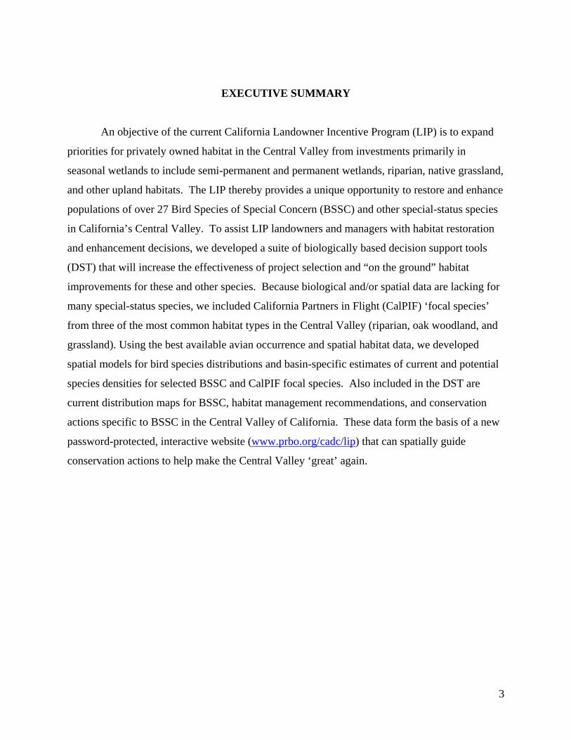
EXECUTIVE SUMMARY
An objective of the current California Landowner Incentive Program (LIP) is to expand
priorities for privately owned habitat in the Central Valley from investments primarily in
seasonal wetlands to include semi-permanent and permanent wetlands, riparian, native grassland,
and other upland habitats. The LIP thereby provides a unique opportunity to restore and enhance
populations of over 27 Bird Species of Special Concern (BSSC) and other special-status species
in California’s Central Valley. To assist LIP landowners and managers with habitat restoration
and enhancement decisions, we developed a suite of biologically based decision support tools
(DST) that will increase the effectiveness of project selection and “on the ground” habitat
improvements for these and other species. Because biological and/or spatial data are lacking for
many special-status species, we included California Partners in Flight (CalPIF) ‘focal species’
from three of the most common habitat types in the Central Valley (riparian, oak woodland, and
grassland). Using the best available avian occurrence and spatial habitat data, we developed
spatial models for bird species distributions and basin-specific estimates of current and potential
species densities for selected BSSC and CalPIF focal species. Also included in the DST are
current distribution maps for BSSC, habitat management recommendations, and conservation
actions specific to BSSC in the Central Valley of California. These data form the basis of a new
password-protected, interactive website (www.prbo.org/cadc/lip) that can spatially guide
conservation actions to help make the Central Valley ‘great’ again.
3

LIST OF FIGURES
Bird Species of Special Concern distribution maps
Figure 1 Fulvous Whistling-Duck
Figure 2 Tule Greater White-fronted Goose
Figure 3 Redhead
Figure 4 American White Pelican
Figure 5 Least Bittern
Figure 6 Snowy Plover
Figure 7 Black Tern
Figure 8 Modesto Song Sparrow
Figure 9 Yellow-headed Blackbird
Figure 10 Northern Harrier
Figure 11 Lesser Sandhill Crane
Figure 12 Short-eared Owl
Figure 13 Tricolored Blackbird
Figure 14 Mountain Plover
Figure 15 Burrowing Owl
Figure 16 Oregon Vesper Sparrow
Figure 17 Grasshopper Sparrow
Figure 18 Yellow-breasted Chat
Figure 19 Yellow Warbler
Figure 20 Long-eared Owl
Figure 21 Purple Martin
Figure 22 Loggerhead Shrike
Figure 23 San Joaquin Le Conte’s Thrasher
4

Maxent distribution maps
Oak Woodland species
Figure 24 Acorn Woodpecker
Figure 25 Ash-throated Flycatcher
Figure 26 Lark Sparrow
Figure 27 Nuttall's Woodpecker
Figure 28 Oak Titmouse
Figure 29 Western Bluebird
Figure 30 Yellow-billed Magpie
Grassland species
Figure 31 Burrowing Owl
Figure 32 Northern Harrier
Figure 33 Western Meadowlark
Riparian and Wetland species
Figure 34 Black-headed Grosbeak
Figure 35 Blue Grosbeak
Figure 36 Common Yellowthroat
Figure 37 Song Sparrow
Figure 38 Spotted Towhee
Figure 39 Swainson's Hawk
Figure 40 Tricolored Blackbird
Figure 41 Yellow-breasted Chat
Figure 42 Yellow Warbler
Species Groups
Figure 43 Bird Species of Special Concern (BSSC)
Figure 44 Grassland Species
Figure 45 Oak Woodland Species
Figure 46 Riparian Species.
Figure 47 PRBO Point Count Locations
5

LIST OF TABLES
Table 1. Broad-scale Habitat Affinities of Taxa on the List of California Bird Species of Special
Concern 2006 Occurring in the Central Valley
Table 2. Status Designations of Conservation Concern for Birds in the Central Valley from
Various State, Regional, Continental, and Global Assessments
Table 3. Severity of Known Historic and Current Threats in California Affecting Taxa on the
List of California Bird Species of Special Concern 2006 Occurring in the Central Valley
Table 4. Variables Used for Distribution Modeling
Table 5. Model Diagnostics (ROC AUC values)
Table 6. Habitat Groups and Associated WHR Types
Table 7. Focal bird species and associated habitat groups.
Table 8. Current Density Estimates for Species by hydrological unit (basin)
Table 9. Target Density Estimates for each species by hydrological unit (basin)
6

APPENDICES
Appendix 1. List of independent variables selected a priori for each species in the distribution
models.
7

ACKNOWLEDGMENTS
We would like to extend our appreciation to the many field assistants at PRBO
Conservation Science for their assistance with data collection used to build these models and
density estimates. We thank Lyann Comrack and Kevin Hunting of the CA Dept. of Fish and
Game and the authors of the BSSC accounts for allowing the use of the account maps and text.
We also thank Tom Gardali, Mark Kenyon, Dean Kwasney, Nadav Nur, and Dave Smith for
technical, logistical and conceptual support and review. The members and board of PRBO
Conservation Science, the National Science Foundation (grant DBI-0542868), The DMARLOU
Foundation, and an anonymous donor provided financial support in conjunction with a standard
agreement administered by the California Department of Fish Game under the Landowner
Incentive Program.
8

CHAPTER 1. CALIFORNIA BIRD SPECIES OF SPECIAL
CONCERN IN THE CENTRAL VALLEY
Background and Introduction
California supports exceptional biodiversity because of its large size, diverse habitats and
environmental heterogeneity, and relative isolation from the rest of the continent (Stein et al.
2000, Stein 2002). In terms of its flora and fauna, California leads the nation in overall species
richness, number of state endemics, and rare species. Along with the possession of such a rich
and diverse bird fauna comes the responsibility for its conservation. Californians must overcome
daunting problems to maintain the state’s biodiversity in the face of severe and ongoing habitat
loss and degradation, which has led to population declines of many native species. California’s
Bird Species of Special Concern (BSSC) list is one of several tools that can be used to help meet
stewardship responsibility for the state’s incredible birdlife, and the habitat it depends on, and to
foster conservation of its at-risk birds.
The BSSC list was first published in 1978 by California Department of Fish and Game
(CDFG) and has been revised two times since (see CDFG 1992), with the most recent revision
being the most substantial. In this most recent permutation, the California BSSC list is based on
a scientifically defensible and repeatable method to set objective standards for inclusion of birds
on the list, for assigning them to different levels of conservation priority, and for forming the
basis for assigning them research priority. The revision also incorporated over twenty years of
data to enable identification of currently declining or vulnerable birds that may warrant listing as
state threatened or endangered if present trends continue. For a definition of a BSSC as well as
detailed explanation of variables considered for listing and special status categorization, see
Shuford and Gardali in press.
As a regulatory tool, the special concern list is intended to guide state, federal, and local
governments in defining the “sensitive” species under the California Environmental Quality Act
(CEQA) for which analysis of project impacts is required. The special concern list is also meant
to stimulate further research, conservation actions, and prevent future listing under state and
federal endangered species acts.
For ease of access to BSSC 2006 information and recommendations that are relevant to
future Landowner Incentive Program (LIP) planning efforts in the Central Valley, we have
9

synthesized threats and habitat recommendations for each species regularly occurring in the
Valley. These are grouped by general habitat type (Table 1) and are derived primarily from
individually authored species accounts. We also include brief summary information for other
special status species regularly occurring in the Central Valley, specifically those federally or
state listed, on the U.S. Fish and Wildlife Service’s (USFWS) list of Birds of Conservation
Concern 2002 (USFWS 2002), or on The International Union for the Conservation of Nature and
Natural Resources’ (IUCN) Red List (see Table 2 for full list). The species highlighted in this
document are those that we believe have great potential to benefit from targeted conservation
activities of private lands habitat programs.
Needs and Challenges
Estimates indicate that California has lost over 90% of its original wetlands (Dahl et al.
1991), 95% of its riparian habitat (RHJV 2004), and 60% of its grasslands (CPIF 2000).
Although biologists frequently emphasize these high rates, the percentages hide the true extent
and complexity of the loss both in terms of structure and function. Habitat degradation and
fragmentation can also have profound effects on biodiversity (Saunders et al. 1991, Debinski and
Holt 2000). Severity of threats affecting BSSC taxa are listed in Table 3.
Among the greatest losses of ecosystem function affecting birds in California is that of
natural hydrology, which before human intervention greatly enhanced biological productivity
both in space and time. The periodic flooding of areas such as the Central Valley formerly
formed a diverse mosaic of permanent and ephemeral wetland and riparian habitats that
depended on such perturbations for renewal (Rosenberg et al. 1991, Shuford et al. 2001).
Restoring natural functions to such habitats will be among the greatest conservation challenges
in the state, though models exist for ways to meet human needs and also conserve the ecological
integrity of riverine ecosystems (Richter and Richter 2000).
The conservation of biodiversity in California faces great challenges because regions of
the state with high numbers of special concern taxa also have the highest human population
densities and projected future growth rates. In the Central Valley, projected growth will be
particularly high in the Sacramento-Yolo county area, qualifying it as a “hotspot of
vulnerability,” i.e., an area with both restricted-range species and high projected rates of human
population growth and development (Abbitt et al. 2000). Likewise, urbanization continues to
10

reduce agricultural lands in the Central Valley at a rate among the highest in North America
(American Farmland Trust 1995, Sorensen et al. 1997).
Protection, restoration, and enhancement of habitats for at-risk species will of necessity
take a multi-faceted approach. A high priority should be placed on protecting natural processes
and species, subspecies, and distinct populations that are nearing endangerment because of
declining populations or vulnerability to threats. The identification of such taxa by California’s
BSSC 2006 list provides a starting point from which to work regardless of the method of
protection selected. Success will be enhanced if efforts are intensified before populations decline
further and if they emphasize voluntary rather than regulatory measures. Such methods include
public and private land acquisition, conservation easements, tax incentives, and cost-share
programs for habitat enhancement (Bean 2000). Cooperative and proactive efforts among
agencies and other groups and between habitat managers and scientists tend to be the most
effective in sensitive species protection (Squires et al. 1998).
Management Recommendations
Except where noted, the following management recommendations are derived from the
California BSSC 2006 species accounts (Shuford and Gardali in press).
WETLANDS
Fulvous Whistling-Duck (Fig. 1; figures begin on page 42)
This species is currently so rare (and irregular) in the San Joaquin Valley that it will be
challenging to manage effectively for it on private lands in that region.
• Protect occupied and potentially suitable nesting and foraging areas and restore or create
additional habitat. Requirements are freshwater marshes with dense stands of emergent
vegetation and open-water areas with floating aquatic plants.
• Maintain water in semi-permanent wetlands until at least mid-August to accommodate this
late-nesting species.
• Consider flooding additional wetlands in the San Joaquin Valley, particularly on federal and
state refuges, through the spring and summer, while identifying and preserving areas suitable
for foraging and nesting.
• Investigate the feasibility of implement Peters’ (2000) proposal to transplant Fulvous
11
Whistling-Ducks from Louisiana to sites in the San Joaquin Valley over a three-year period,
after determining the best potential release sites. Future management of such sites should
emphasize the actions specified above that promote the maintenance of viable whistling-duck
populations into the future.
Tule Greater White-fronted Goose (Fig. 2)
• Protect or enhance relatively deep marshes dominated by tules and bulrushes (Scirpus spp.)
and cattails (Typha spp.) in the known range of the tule greater white-fronted goose in the
Sacramento Valley. Protect areas with a mosaic of harvested rice fields, used early in fall
and during hunting season (late Oct-late Jan), and winter-flooded uplands and marshes with
an abundance of Alkali Bulrush (Scirpus robustus) and some open water, used later in the
season.
• Provide some open water ponds with some emergent vegetation where Tule Geese can roost
and loaf.
• Identify additional habitat outside the federal and state refuges for possible protection.
• Continue restrictive hunting regulations in the core wintering range with mid-December
closures until the population levels and trends are better known.
Redhead (Fig. 3)
• Where feasible, increase the extent of permanent and semi-permanent, deep-water (>1 m)
marshes to provide suitable Redhead breeding habitat. Optimally, such wetlands should be
>0.4 ha in extent and offer a mosaic of about 75% open water interspersed with dense
emergent vegetation.
• Work for allocation of adequate water supplies to allow for management of suitable
wetlands; use state and federal incentive programs to promote permanent and semi-
permanent wetlands on private lands.
American White Pelican (Fig. 4)
Because this species has not bred in the Central Valley since the early 1950s, it would
take extraordinary efforts to restore isolated, fish-productive wetlands of sufficient size to
reestablish a nesting colony in this region. Still, restoration or enhancement of large wetlands
might benefit pelicans in the region during winter and migration.
12
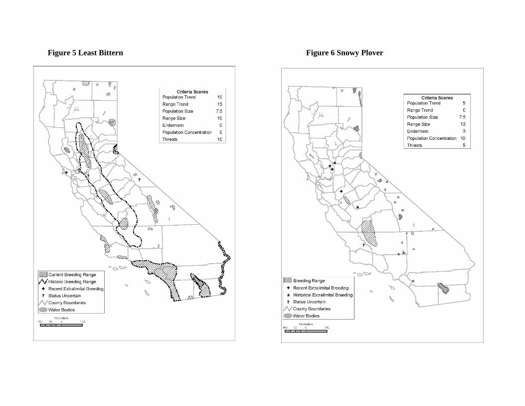
Least Bittern (Fig. 5)
• Preserve, protect, and improve shallow marshes (>10 ha in size) that contain dense emergent
vegetation.
• Protect existing patches of habitat used by Least Bitterns at sites identified as occupied
habitat on the basis of recent records or future monitoring efforts.
• Manage summer wetlands to increase the availability of suitable bittern habitat by extending,
where feasible, the current four-year cycle for refuge marsh management to one of about
seven years.
• Minimize disturbance to Least Bitterns during their nesting season.
Snowy Plover (Fig. 6)
• Focus on protecting and enhancing important breeding sites by first determining source areas
for the overall population that produce young above the levels needed to replace adult
mortality. In the meantime, protect or enhance all sites that currently support at least five
pairs of breeding plovers and evaluate the feasibility of enhancing habitat at sites holding
fewer pairs.
• Ensure that breeding areas receive adequate high-quality water (lacking high levels of
contaminants or selenium) and that water diversions do not eliminate or degrade important
nesting habitats.
• Protect, enhance, or restore habitats that may be negatively impacted or threatened by water
management practices, such as spring draw downs that remove foraging areas needed by
breeding plovers.
• Ensure that regional efforts to restore wetlands in the southern San Joaquin Valley include
creation of some playa lake habitats suitable for plovers, not just freshwater wetlands.
• Protect key stopover and wintering areas for Snowy Plovers, such as San Joaquin Valley
evaporation ponds, or provide suitable alternative habitat nearby using water with low
selenimum concentrations.
13
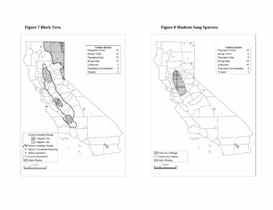
Black Tern (Fig. 7)
• Focus on restoring, enhancing, and providing long-term protection for suitable early
successional wetlands and on maintaining isolation of colonies from humans and ground
predators.
• Consider eliminating early-season draw downs in rice fields to reduce the likelihood of
predation of tern nests.
• Consider enhancing tern habitat primarily in years of exceptional runoff, when it will do the
most good, thereby exploiting the tendency of seabirds to exhibit boom and bust cycles of
productivity. In such years, try to increase limited breeding on newly restored wetlands on
refuges near Los Banos by spreading water over larger areas within the Eastside Bypass near
Los Banos and the James Bypass/Fresno Slough south of Mendota Wildlife Area or by
drawing water from upstream, circulating it through refuge ponds, and draining it back into
the bypass downstream. Maintain a slow but steady flow to reduce the chances of botulism.
• When possible, flood fields containing residual vegetation or crop stubble for use as breeding
habitat. Explore retiring fields with marginal crop yields and putting them in a conservation
bank to be flooded when water is available. Weigh such flooding against possible mortality
of waterbirds from botulism disease outbreaks, which might be reduced by rotating fields to
be flooded and choosing areas with no prior evidence of disease.
Modesto Song Sparrow (Fig. 8)
• Protect and create suitable emergent freshwater marshes dominated by tules (Scirpus spp.)
and cattails (Typha spp.), early successional riparian willow (Salix spp.) thickets, young
Valley Oak (Quercus lobata) forests with a sufficient understory of blackberry (Rubus spp.),
and vegetated irrigation canals and levees.
• To counteract the sparrows’ low dispersal capabilities, create new habitat close to currently
occupied habitat.
• If possible, implement measures to reduce predation and parasitism of nests such as
increasing plant understory volume.
• Focus management and restoration efforts primarily on identifying and maintaining source
populations capable of producing young in excess of adult mortality.
14
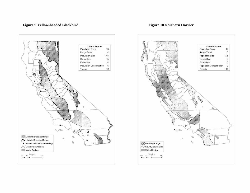
Yellow-headed Blackbird (Fig. 9)
• Protect large, deep-water marshes, particularly those managed with water depth of at least 30
cm under emergent stands of Typha or Scirpus.
• Focus on the enhancement and restoration of suitable wetlands for breeding, particularly
within important historical nesting areas such as the Tulare Basin.
• Manage deepwater marshes to increase or maintain sufficient habitat edges and patchiness
important for nest sites.
WETLANDS AND GRASSLANDS
Northern Harrier (Fig. 10)
• Maintain a mosaic of large undisturbed habitats for nesting and foraging, particularly those
with an abundant prey base, e.g., freshwater marshes, abandoned fields, active alfalfa fields,
wet grasslands, and fields with dense green and residual vegetation.
• Minimize human disturbance near nesting areas, restricting public access as necessary during
the breeding season.
• Reduce livestock impacts on nesting success by limiting their access to harrier nesting areas,
especially during the breeding season.
• Practice rest-rotational range management, leaving some sections idle each year.
• Delay haying and plowing when possible until after nestlings have fledged (~ mid July).
• Avoid raising wetland water levels during the nesting season to prevent flooding nests of
harriers and other ground-nesting species.
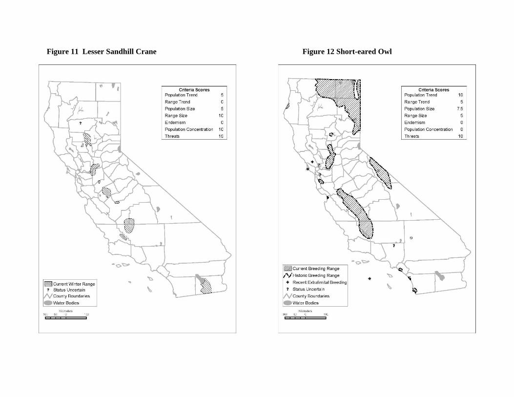
Lesser Sandhill Crane (Fig. 11)
The following recommendations will also benefit the Greater Sandhill Crane (G. c.
tabida), a state threatened species. However, Greaters are more constrained by distance of
foraging sites from their roost sites (Ivey and Herziger 2003) - on average traveling less than 2
miles to forage. For specific locations of conservation priority in regions of the Central Valley,
see Ivey 2005. Additionally, CDFG is required to implement a Greater Sandhill Crane Recovery
Strategy and Pilot Program by 2009.
• Protect and enhance favorable grain crops and provide unharvested corn and milo plots on
15
federal, state, and other conservation lands used by Lesser Sandhill Cranes in the Central
Valley. Consider purchase or easements on major feeding areas in Merced, San Joaquin, and
other counties where major crane use areas are discovered or established.
• Encourage farmers to delay discing grain crop stubble until after February, as deep discing
buries waste grains.
• Similarly, encourage farmers and wildlife agency personnel to delay burning or flooding of
grain stubble until late February.
• Encourage management of row crops to provide nut sedge, a highly desired food resource in
row crops, in the fall and winter.
• Protect and enhance shallow, sparsely vegetated wetlands within 2-4 km of major crane
feeding areas to provide favorable roosting and loafing sites.
• Minimize disturbance to crane roosting and foraging habitats and prioritize sites with
minimal or no disturbance for conservation efforts.
• Limit all hunting activities within 0.4 km of crane roost sites and other use areas, and, where
possible, restrict human access.
• Manage 20%-40% of grasslands in major crane use areas with cattle grazing to provide
foraging sites for cranes.
• To avoid collisions, reroute any utility corridor proposed through crane use areas.
Short-eared Owl (Fig. 12)
Management for voles or other cyclic prey needed by these owls may take
experimentation and hence may be difficult to implement on private lands in the short term.
• Protect freshwater marshes and grasslands.
• Implement and monitor management practices on wildlife refuges and agricultural lands that
are conducive to both vole and Short-eared Owl productivity, realizing that, because of the
cycles of both, obvious benefits may not be realized every year.
• Maintain a mosaic of habitats with lush herbaceous vegetation, including sufficient areas of
weedy abandoned fields and wet grasslands; as appropriate, leave some areas ungrazed.
• Implement predator control programs where necessary, particularly to eliminate non-native
ground predators such as the Red Fox.
• Avoid flooding fields or wetlands where owls are known or suspected to be nesting.
16
• Encourage rest-rotational schemes on cattle-grazed or agricultural fields that leave some land
in lush herbaceous vegetation each spring.
• Minimize hay mowing and crop harvesting during the breeding season (particularly March-
May) in fields that have sufficient cover (30-60 cm high) to support breeding owls, or mow
around known nests if they are found.
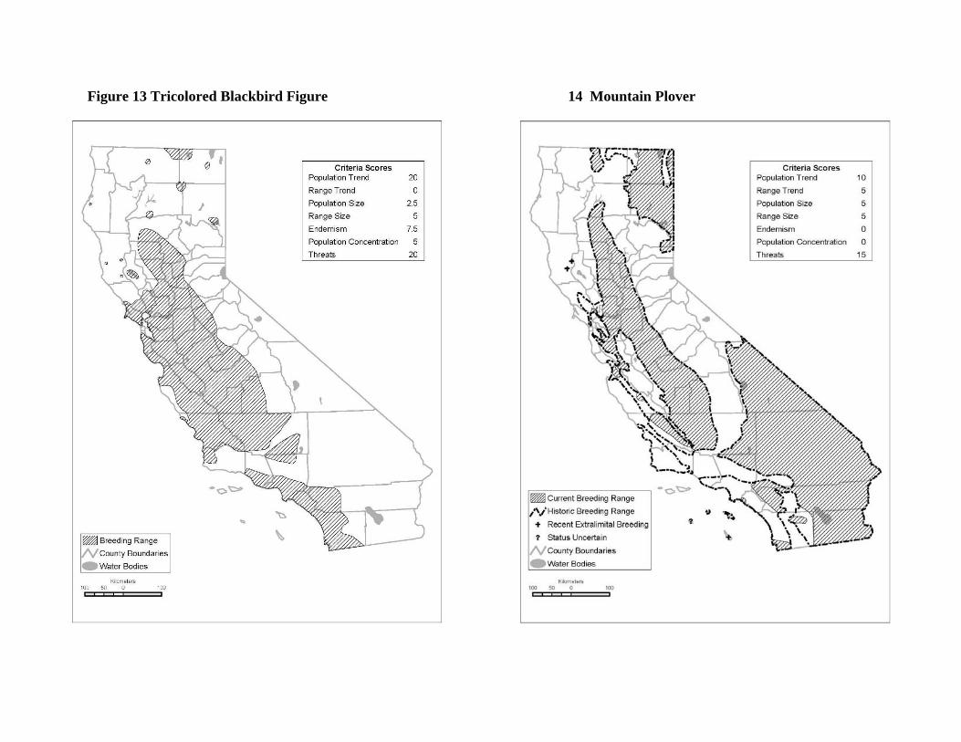
Tricolored Blackbird (Fig. 13)
In addition to the management recommendations from the BSSC, a “Conservation
Strategy for the Tricolored Blackbird” document has been produced by the Tricolored Blackbird
Working Group (2007). More detailed recommendations are included in that report, which
should be consulted to direct conservation action.
• Restore habitat by promoting the growth of secure nesting substrates (e.g., nettles, thistles,
and other naturally armored native plants) near productive foraging habitats to increase the
potential carrying capacity for this species. Restored nesting habitats should be situated on
protected public and private lands, especially in agricultural areas of the Central Valley and
surrounding foothills.
• On refuges and other public lands that support Tricolored Blackbird colonies in irrigated
pastures, manage irrigation to permit a sequential flooding regime in adjacent land parcels at
the time they are breeding to enhance insect productivity. Incorporate carefully managed
grazing of these parcels to maintain an average vegetation height of 15 cm to provide optimal
Tricolored Blackbird foraging habitat.
• Lure nesting Tricolored Blackbirds, when possible, away from dairies and other agricultural
operations to secure habitats where they are more likely to succeed; where colonies establish,
defer harvest of grain and silage crops, if feasible, until after the breeding season.
GRASSLANDS
Mountain Plover (Fig. 14)
• Protect traditional wintering sites and high-quality wintering habitat from urban development
and other incompatible land use changes by securing conservation easements and property
acquisition as part of regional conservation planning efforts. Prime sites are short-grass
prairie habitats, or their equivalents, that are flat and nearly devoid of vegetation; in winter
17

these include fallow, heavily grazed, or recently burned sites.
• Manage grassland habitat, where possible, to maintain low stature and cover of grass. Time
controlled burns to accommodate mid-winter Mountain Plover use.
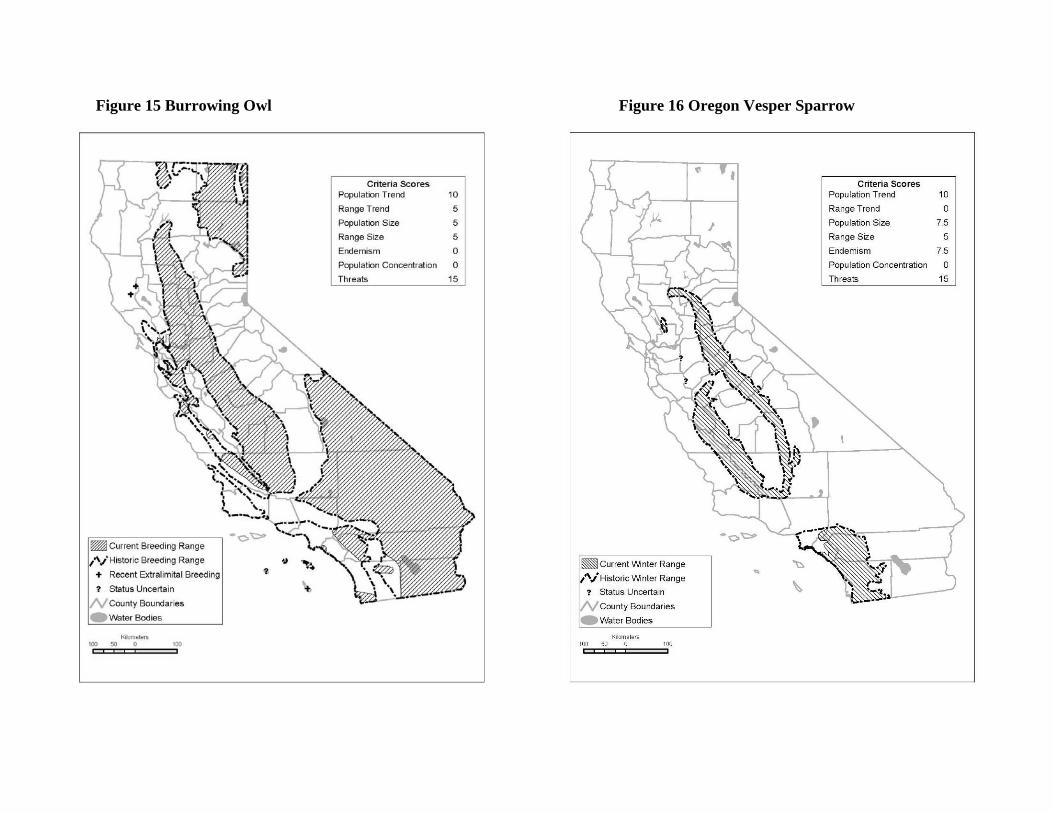
Burrowing Owl (Fig. 15)
The following recommendations pertinent to non-breeding habitat also would likely
benefit Ferruginous Hawk – an IUCN “near threatened” species:
• Place sizeable tracts of grassland under conservation easements or agreements with
agricultural (grazing) operations to maintain populations through best management practices,
such as the elimination or restriction of small mammal poisoning.
• Conservation agreements should also be sought with landowners of row crop agriculture, to
encourage appropriate management of water conveyance structures, roadsides, and field
margins. It will be necessary to work closely with landowners to alleviate concerns that
maintaining owls on their property is a liability in terms of flexibility in land management
practices necessary to maintain economic viability.
• Maintain suitable vegetation structure through mowing, revegetate with low-growing and
less dense native plants, or controlled grazing, as appropriate.
• Where nesting burrows are lacking, enhance habitat by using artificial burrows or
encouraging the presence of ground squirrels.
• Control off-road vehicles and unleashed pets within occupied Burrowing Owl habitat.
• Develop prescriptions that mimic natural processes and that preferably do not require
ongoing management for maintaining Burrowing Owls.
Oregon Vesper Sparrow (Fig. 16)
• Preserve grassland areas known to support high numbers of Vesper Sparrows in winter,
using purchase, easements, and incentives as necessary or possible. Prime areas typically
have open ground with little vegetation or are grown to short grass and low annuals; these
include stubble fields, meadows, and road edges.
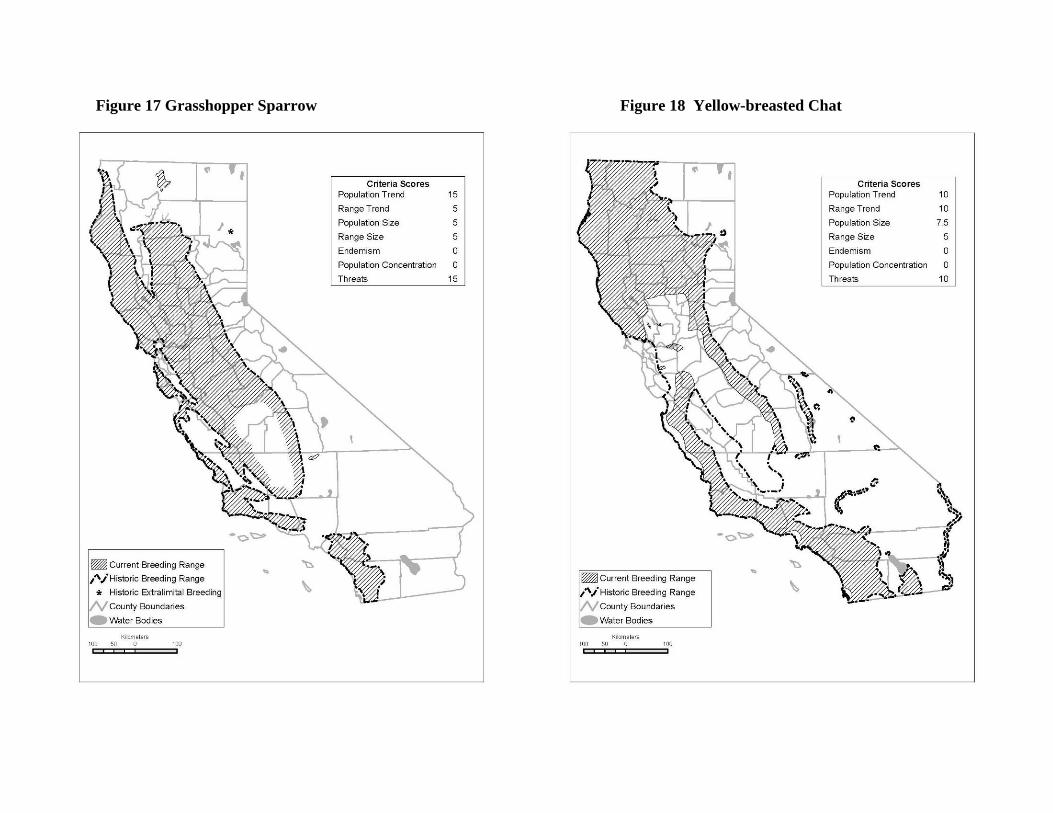
Grasshopper Sparrow (Fig. 17)
Because this species is extirpated as a breeding bird in the southern San Joaquin Valley,
and generally is a very rare and local breeder in grasslands in the rest of the Central Valley, it
18
likely will be difficult to manage for it on private lands in California until future research can
identify the characteristics of grassland that are needed to support this species in this region.
• Protect or restore large tracts of short to middle-height, moderately open grasslands with
scattered shrubs.
• Negotiate conservation agreements (allowing limited grazing, for example, but preserving
grassland) or favorable zoning on private land.
• Redirect urbanization away from native and non-native grasslands.
• Manage as native grassland significant tracts of Grasshopper Sparrow habitat that come into
public ownership.
• Minimize or prevent disturbance of the ground surface in native grassland, as this favors
exotic weeds at the expense of native grasses. Develop means for restoring native grassland.
GRASSLANDS AND RIPARIAN HABITAT
Swainson’s Hawk (from Woodbridge 1998)
The primary management issues currently facing Swainson’s Hawks in California are: 1)
loss of preferred nesting habitat in mature riparian forest; 2) loss or adverse modification of
high-quality foraging habitat to development or conversion to incompatible crop types; and 3)
high mortality due to pesticide use on migration route and wintering areas. Over 95% of the
known nest sites are on private lands and are vulnerable to changes in the agricultural
environment and development. The Swainson’s Hawk Technical Advisory Committee (SWTAC)
has been particularly active in the three primary Swainson’s Hawk population centers in the
Central Valley – Sacramento, San Joaquin, and Yolo counties. The SWTAC is currently
developing a recovery plan for the species, which should provide more specific habitat
management recommendations for the Valley. In the interim, general recommendations include:
• Ensure the availability of suitable nesting and foraging habitat through preservation of
riparian systems and groves of, or lone, mature trees in agricultural fields.
• Maintain compatible agricultural practices in grasslands, pastures, and croplands.
• Optimize adjacency of the above two elements.
• Protection and restoration of riparian forests may provide nesting habitat superior to other
sources of trees such as roadsides and field margins.
19
• Protection and restoration of riparian systems even along smaller drainages (e.g., Willow
Slough – Woodland, and Red Bridge Slough – Vernalis) would provide numerous nesting
opportunities.
• Provide incentives for Swainson’s Hawk friendly agricultural practices (e.g., maintain fallow
lands, lightly grazed pastures) or to grow specific crops (e.g., alfalfa and other hay crops) vs.
unsuitable crops (e.g., vineyards, orchards, and cotton).
RIPARIAN HABITAT
Yellow-breasted Chat (Fig. 18)
• Preserve existing, and restore degraded, riparian habitat, particularly early successional
habitats, with a well-developed shrub layer and an open tree canopy, that are restricted to the
narrow border of streams, creeks, sloughs, and rivers.
• Manage riparian habitat to maintain and/or promote a dense shrub layer; install a shrub layer
in the early stages of restoration projects.
• Time removal of exotic plants from riparian areas used by nesting chats to avoid disturbance
during breeding(April-August), and proceed only after careful assessment and mitigation for
any potential detrimental effects to chats.
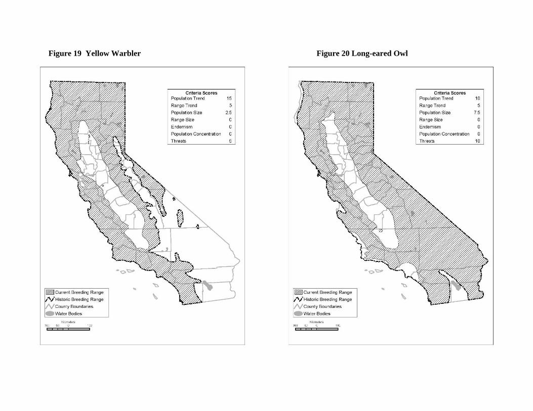
Yellow Warbler (Fig. 19)
• Protect, manage, and restore dynamic riparian systems that provide the mechanisms (e.g.,
seasonal flooding) to create early successional as well as more structurally complex
vegetative components (e.g., herbaceous cover, shrub cover, and riparian tree canopy).
• Eliminate or manage cowbird feeding sites near Yellow Warbler breeding habitat.
• Cowbird trapping may be a viable option to aid warblers in some areas, but criteria outlined
by experts (Smith 1999, NACAC 2003) should be met prior to the initiation of any trapping
program.
Yellow-billed Cuckoo (from Laymon 1998)
• All existing habitat should be preserved regardless of present habitat quality, and low quality
habitat should be enhanced to reach suitable or optimal levels.
• Sites capable of producing optimal habitat should receive highest priority for restoration.
20

• The best habitats for nesting are at large sites with high canopy cover and foliage volume,
and moderately large and tall trees. Specifically:
Sites >80 ha in extent and wider than 600 m are optimal habitat. Sites 41-80 ha in
extent and wider than 200 m are suitable, and sites 20-40 ha and 100-200 m-wide
are marginal.
Sites with greater than 65% tree canopy closure are optimal. Sites with 40-65%
are marginal to suitable.
Sites with foliage volume from 30,000 m3/ha to 90,000 m3/ha are optimal. Sites
with 20,000 m3/ha to 30,000 m3/ha, and over 90,000 m3/ha are suitable.
Sites with mean canopy height 7-10 m may be optimal. Sites with mean canopy
height from 4-7 m and from 10-15 m appear to be suitable.
Nest sites with basal area (cross-sectional area of all the trees at breast height per
hectare of forest) between 5 m2/ha and 20 m2/ha appear to be optimal. Sites with
basal area 20 m2/ha to 55 m2/ha are suitable. Sites with basal area less than 5
m2/ha and greater than 55 m2/ha are marginal.
• Restoration efforts should be concentrated in areas adjacent to existing habitat patches, or in
areas of sufficient extent to create comparatively larger tracts of habitat.
• Restoration efforts in the southern portion of the nesting range should be higher priority (e.g.,
South Fork of the Kern River) but northern sites also essential (e.g., Sacramento River from
Red Bluff to Colusa; RHJV 2000).
• Restore and protect adjacent upland refugia habitats for foraging in wet years, as primary
prey species hibernate underground and are not available in wet years with late spring
flooding.
Least Bell’s Vireo
This species is currently so rare (perhaps only a single pair) in the Central Valley that it
may be extremely difficult to manage effectively for it on private lands in that region. However,
riparian habitat restoration has the potential to increase the vireo population and further
expansion into the Valley. Least Bell’s Vireos prefer early successional riparian areas (RHJV
2000).
21
Bank Swallow (from Garrison 1998)
A recovery plan has been written for the Bank Swallow in California (Schlorff 1992).
The most significant management issue affecting the Bank Swallow in California is the direct
loss of suitable colony sites through bank protection and flood control projects, particularly on
the Sacramento River (Garrison et al. 1987).
• Conservation of extensive amounts of suitable nesting sites throughout large areas is
important for success.
• Integrating Bank Swallow habitat protection with larger scale riparian ecosystem
conservation efforts is promising.
• Cycles of flooding and erosion should be allowed to continue in as naturally cycle as
possible.
• Local breeding populations benefit greatly from annual erosion to create new nesting habitat
and maintenance of suitable banks, cliffs, and bluffs where nesting colonies already occur.
• Artificial habitat enhancement is not very cost-effective and may not be necessary in areas
where considerable amounts of suitable habitat exist.
RIPARIAN AND OAK WOODLAND
Long-eared Owl (Fig. 20)
Because this species has declined and is now a very scarce and irregular breeder in the
Central Valley, it likely will prove difficult currently to effectively manage for this species on
private lands. As with Short-eared Owls, management for voles or other cyclic prey needed by
Long-eared Owls may take experimentation and hence may be difficult to implement on private
lands in the short term.
• Protect and enhance riparian forests and oak woodlands adjacent to grasslands, meadows, or
shrublands, particularly areas of known breeding occurrence with suitable adjacent foraging
habitat giving special attention to appropriate vegetative cover and configuration and
considering the surrounding landscape out to 3 km from core nesting areas.
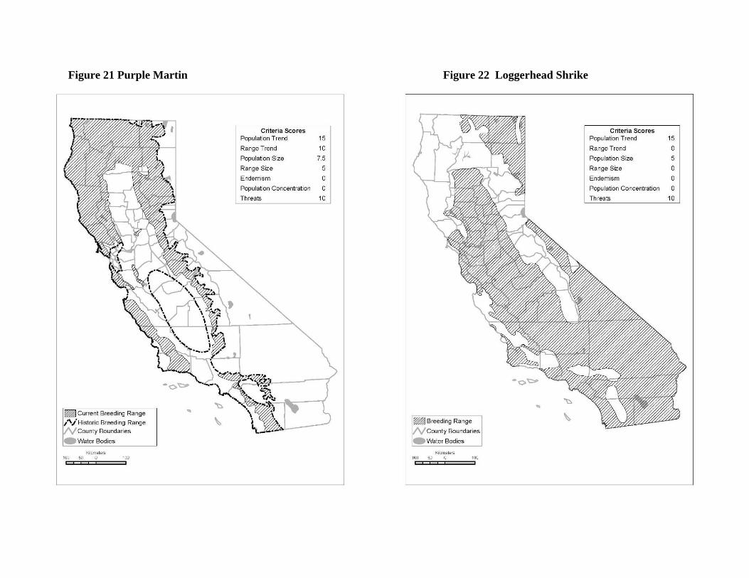
Purple Martin (Fig. 21)
Before the arrival and increase of European Starlings, fierce competitors for nest
cavities, Purple Martins formerly nested in buildings and riparian habitats from Stockton in the
22
Delta north through the Sacramento Valley. Martins now breed in this region only in the city of
Sacramento, where they have persisted by nesting in hollow-box bridges. Hence, management
for martins in this region is likely to be effective only by protecting, enhancing, or creating
artificial nesting sites.
• Protect occupied and suitable bridge sites from uses that restrict air space and martin access or
that cause excessive human disturbance.
• Establish nest box programs to diversify nesting habitats where nest-site competition threatens
or has eliminated martins and where commitment to long-term management is certain. Do not
foster complete conversion to nest boxes for populations that are successfully nesting in trees,
bridges, or power poles.
SHRUBLANDS
Loggerhead Shrike (Fig. 22)
• Maintain and increase suitable breeding habitat of shrublands or open woodlands with tall
shrubs or trees (also fences) for hunting perches; open areas of short grasses, forbs, or bare
ground for prey capture; and large shrubs or trees for nest placement.
• Continue efforts to curb conversion of native shrub habitats to exotic plant communities or
agricultural fields.
San Joaquin Le Conte’s Thrasher (Fig. 23)
• Protect and maintain all existing Le Conte’s Thrasher habitats in the San Joaquin Valley.
These typically are on gentle to rolling, well-drained slopes bisected with dry washes,
conditions found most often on bajadas or alluvial fans. Occupied habitats are generally
moderately to sparsely-vegetated by saltbush with bare ground or patches of sparse low-
growing grass. Foraging areas are well-drained and have extensive bare ground and a well-
developed litter layer near shrubs; nesting areas require at least a few larger, dense shrubs for
nest placement.
• Target habitat restoration toward lost or degraded sites, particularly saltbush habitat in large
areas destroyed by fire (e.g., Lokern Natural Area).
• Create habitat corridors within and among subpopulations.
• Maintain, at a minimum, corridors of intact habitat through oil fields along properly
23

functioning drainages in the McKittrick-Maricopa and Lost Hills areas.
• Allow grazing by livestock for part of the year to benefit saltbush habitat by reducing fire,
which otherwise can spread and intensify non-native annual plant matter. Set livestock
stocking rates at a level such that the majority of shrubs maintain a near hemispherical shape.
Restrict the season of use to when there is adequate green vegetation for livestock to select
grasses, thereby minimizing use of saltbush. Do not allow grazing of saltbush habitat during
prolonged drought, or for a year following a significant recruitment of seedlings.
24
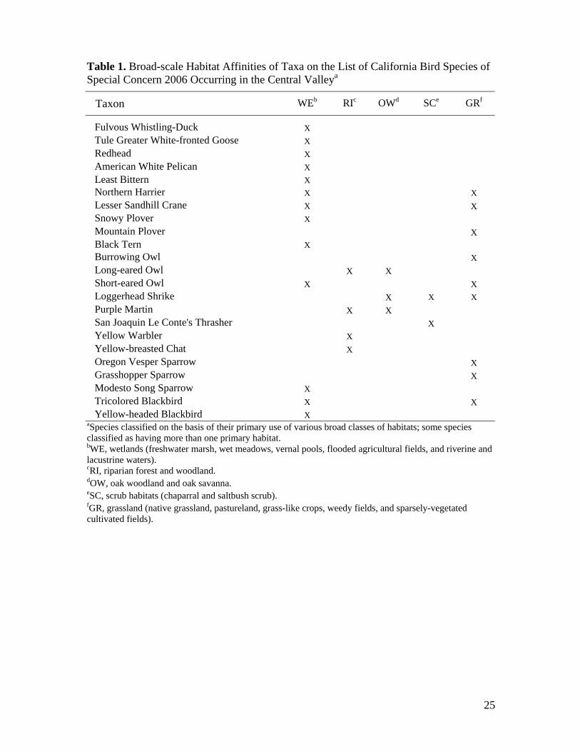
Table 1. Broad-scale Habitat Affinities of Taxa on the List of California Bird Species of Special Concern 2006 Occurring in the Central Valleya
Taxon WEb RIc OWd SCe GRf
Fulvous Whistling-Duck X Tule Greater White-fronted Goose X Redhead X American White Pelican X Least Bittern X Northern Harrier X X Lesser Sandhill Crane X X Snowy Plover X Mountain Plover X Black Tern X Burrowing Owl X Long-eared Owl X X Short-eared Owl X X Loggerhead Shrike X X X Purple Martin X X San Joaquin Le Conte's Thrasher X Yellow Warbler X Yellow-breasted Chat X Oregon Vesper Sparrow X Grasshopper Sparrow X Modesto Song Sparrow X Tricolored Blackbird X X Yellow-headed Blackbird X aSpecies classified on the basis of their primary use of various broad classes of habitats; some species classified as having more than one primary habitat. bWE, wetlands (freshwater marsh, wet meadows, vernal pools, flooded agricultural fields, and riverine and lacustrine waters). cRI, riparian forest and woodland. dOW, oak woodland and oak savanna. eSC, scrub habitats (chaparral and saltbush scrub). fGR, grassland (native grassland, pastureland, grass-like crops, weedy fields, and sparsely-vegetated cultivated fields).
25
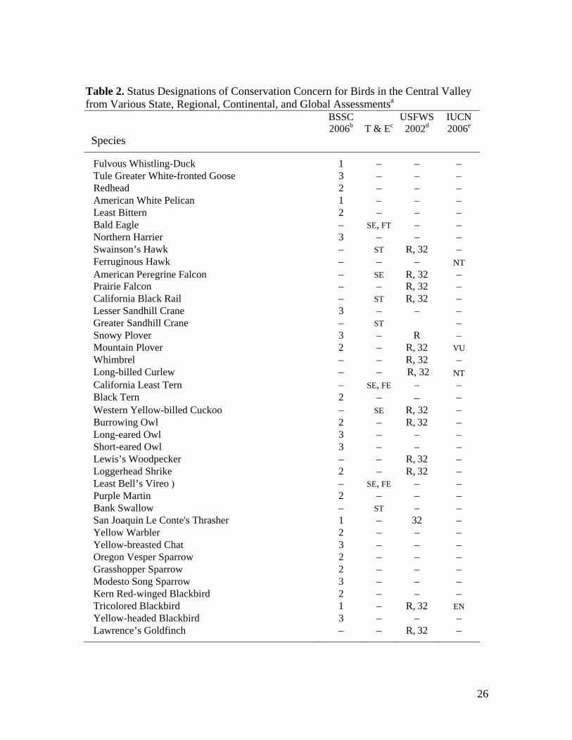
Table 2. Status Designations of Conservation Concern for Birds in the Central Valley from Various State, Regional, Continental, and Global Assessmentsa
Species
BSSC 2006b
T & Ec
USFWS 2002d
IUCN 2006e
Fulvous Whistling-Duck 1 – – – Tule Greater White-fronted Goose 3 – – – Redhead 2 – – – American White Pelican 1 – – – Least Bittern 2 – – – Bald Eagle – SE, FT – – Northern Harrier 3 – – – Swainson’s Hawk – ST R, 32 – Ferruginous Hawk – – – NT American Peregrine Falcon – SE R, 32 – Prairie Falcon – – R, 32 – California Black Rail – ST R, 32 – Lesser Sandhill Crane 3 – – – Greater Sandhill Crane – ST – Snowy Plover 3 – R – Mountain Plover 2 – R, 32 VU Whimbrel – – R, 32 – Long-billed Curlew – – R, 32 NT California Least Tern – SE, FE – – Black Tern 2 – – – Western Yellow-billed Cuckoo – SE R, 32 – Burrowing Owl 2 – R, 32 – Long-eared Owl 3 – – – Short-eared Owl 3 – – – Lewis’s Woodpecker – – R, 32 – Loggerhead Shrike 2 – R, 32 – Least Bell’s Vireo ) – SE, FE – – Purple Martin 2 – – – Bank Swallow – ST – – San Joaquin Le Conte's Thrasher 1 – 32 – Yellow Warbler 2 – – – Yellow-breasted Chat 3 – – – Oregon Vesper Sparrow 2 – – – Grasshopper Sparrow 2 – – – Modesto Song Sparrow 3 – – – Kern Red-winged Blackbird 2 – – – Tricolored Blackbird 1 – R, 32 EN Yellow-headed Blackbird 3 – – – Lawrence’s Goldfinch – – R, 32 –
26
aConservation status designations are provided for comparison of widely cited assessments at various scales, regional to global. Taxa included on other lists are not included here if they occur in the Central Valley only as vagrants or rare migrants or visitors, unless they formerly were much more numerous in the region and subsequently have been greatly reduced in numbers by human activities. For some taxa, rankings may apply to different seasonal or breeding roles on different lists. bSpecies, subspecies, and distinct populations on the 2006 list of California Bird Species of Special Concern (Shuford and Gardali in press) that occur in the Central Valley. Numbered designations indicate priority levels within the list (1, 2, or 3; highest to lowest). cSpecies listed as threatened or endangered by state or federal law. ST, state threatened; SE, state endangered; FT, federally threatened; FE, federally endangered. dSpecies or subspecies on the USFWS list of Birds of Conservation Concern 2002 (USFWS 2002); includes taxa of lesser concern than those listed as Federally threatened or endangered (see footnote c above). R, USFWS Region 1 (states of CA, HI, ID, NV, OR, and WA, plus other Pacific islands). The number 32 refers to Bird Conservation Region 32 (Coastal California), which includes the Central Valley. eCentral Valley species with IUCN Red List global conservation status ranks (listed here in descending order of conservation concern): CR, critically endangered; EN, endangered; VU, vulnerable; and NT, near threatened (IUCN 2006).
27
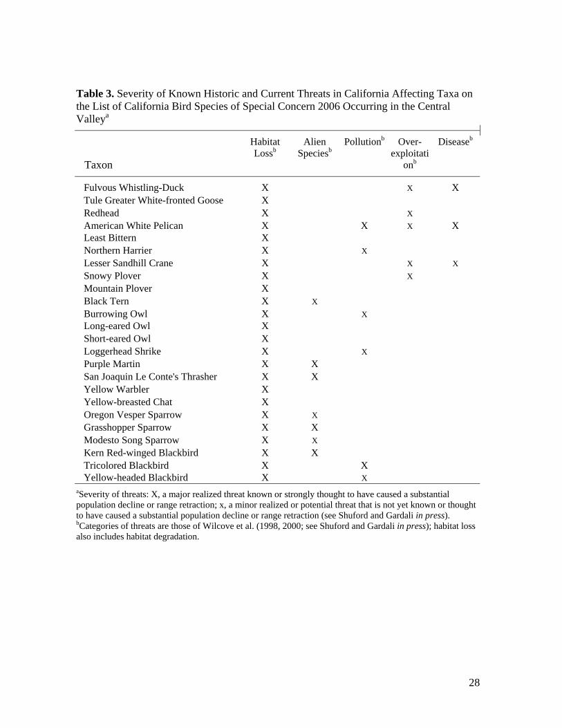
Table 3. Severity of Known Historic and Current Threats in California Affecting Taxa on the List of California Bird Species of Special Concern 2006 Occurring in the Central Valleya
Taxon
Habitat Lossb
Alien Speciesb
Pollutionb Over- exploitati
onb
Diseaseb
Fulvous Whistling-Duck X X X Tule Greater White-fronted Goose X Redhead X X American White Pelican X X X X Least Bittern X Northern Harrier X X Lesser Sandhill Crane X X X Snowy Plover X X Mountain Plover X Black Tern X X Burrowing Owl X X Long-eared Owl X Short-eared Owl X Loggerhead Shrike X X Purple Martin X X San Joaquin Le Conte's Thrasher X X Yellow Warbler X Yellow-breasted Chat X Oregon Vesper Sparrow X X Grasshopper Sparrow X X Modesto Song Sparrow X X Kern Red-winged Blackbird X X Tricolored Blackbird X X Yellow-headed Blackbird X X aSeverity of threats: X, a major realized threat known or strongly thought to have caused a substantial population decline or range retraction; x, a minor realized or potential threat that is not yet known or thought to have caused a substantial population decline or range retraction (see Shuford and Gardali in press). bCategories of threats are those of Wilcove et al. (1998, 2000; see Shuford and Gardali in press); habitat loss also includes habitat degradation.
28
CHAPTER 2. DECISION SUPPORT TOOLS
Introduction
An objective of the current California LIP is to expand habitat priorities in the Central
Valley from primarily seasonal wetland investments to semi-permanent and permanent
wetlands, riparian, native grassland, and other upland habitats (e.g., oak woodland) and
thereby expand the program’s benefits to the multitude of special status species known to
occur throughout the Central Valley. Building on the numerous partnerships currently being
established between private landowners, state and federal agencies, and non-governmental
organizations, this LIP program provides the opportunity to restore and enhance populations
of over 27 Bird Species of Special Concern (BSSC) and other special status species. BSSC
species, as described above, are from the most recent list revised in 2006, which was based
on a scientifically defensible and repeatable methodology. These species warrant immediate
conservation action to prevent further regulatory actions. For more information see Shuford
and Gardali (in press).
Because current biological data on which to base management and planning decisions
are often lacking for many species of concern, we also addressed ‘focal species’ from three
of the most common habitat types in the Central Valley (riparian, oak woodland, and
grassland). These species represent various stages of vegetative succession, habitat
characteristics and/or critical ecosystem elements and have been used previously by
California Partners in Flight (CalPIF) to develop statewide habitat based bird conservation
plans (BCPs, http://www.prbo.org/calpif/plans.html). Thus the implementation of
conservation actions that benefit multiple focal species is assumed to enhance the
biodiversity of the habitat in question, including species of special concern (Chase and
Geupel 2005).
By focusing on BSSC species such as Tricolored Blackbird and Burrowing Owl that
are precariously close to being listed as threatened or endangered, and CalPIF focal species
such as Song Sparrow and Common Yellowthroat that may respond rapidly to restoration
and enhancement, we anticipate an increase in the popularity of the LIP program. Private
landowners will be able to achieve measurable and noticeable population increases, thus
preventing the regulatory polarizations that often accompany endangered species regulations.
29
In this chapter we use current information on BSSC and CalPIF focal species to assist
the planning and implementation of the California LIP program in the Central Valley. We
achieve this by 1) presenting spatially explicit distribution models that predict probability of
occurrence of BSSC and CalPIF focal species, 2) providing current basin-specific focal
species density estimates (birds per hectare) to provide a measurable baseline and potential
target for evaluation of project success, and 3) providing comparative values of nest
survivorship for a subset of focal species to provide insight on population health and
potential growth.
Species Distributions Models as Planning Tools
INTRODUCTION
Program effectiveness may be greatly enhanced by using a consistent and biologically
based method for evaluating and prioritizing actions on the ground. Models of species habitat
associations and spatial predictions of species occurrence (‘species distribution models’) are
a defensible and valuable method to guide where projects should be implemented and what
management prescriptions are needed.
The recent development of sophisticated species distribution modeling techniques
provides an opportunity to greatly improve the value and usefulness of species occurrence
data (Guisan and Zimmermann 2000, Austin 2002). While GIS-based, empirical species
distributional models have been developed at broad spatial scales for over a decade
(Lindenmayer et al. 1991, Pereira and Itami 1991, Aspinall and Veitch 1993), the increasing
availability of comprehensive and detailed vegetation and land use GIS layers has improved
our ability to develop more accurate and detailed models of species occurrence for local and
regional conservation purposes. Species distribution models can provide significant
improvements in predictive abilities over the simple habitat suitability index (HSI) or wildlife
habitat relationship (WHR) models, which are often based on broad-scale habitat associations
that are not necessarily applicable throughout a species’ range. Individual species
distribution models can also be combined in an index of multi-species habitat value.
Furthermore, new and sophisticated modeling algorithms have improved our ability
to predict species distributions based on presence-only occurrence data such as that found in
the California Natural Diversity Database (CNDDB) (Elith et al. 2006, Hernandez et al.
30
2006). Using new statistical and machine learning approaches, point occurrence data can be
related to GIS-based environmental data layers to generate robust, spatially continuous
predictions of species occurrence.
METHODS
Our approach was to use a powerful machine learning algorithm called Maxent
(Phillips et al. 2006) to predict species distributions based on species occurrence locations
and GIS-based environmental data layers. Maxent is based on the principle of maximum
entropy, and uses information about a known set of species occurrence points, compared with
environmental “background” data, to develop parsimonious models of species occurrence.
The method accommodates several different types of non-linear relationships and is similar
to generalized additive models (Hastie and Tibshirani 1990) in its outputs and interpretation.
Species occurrence data came from two different datasets: (1) the California Natural
Diversity Database (CNDDB), and (2) PRBO’s long-term avian point count survey database,
including over 7,000 points throughout California (Fig 47). We used the CNDDB data to
model many of the BSSC species that are not well-captured by point count surveys (i.e., non-
passerine species). For other species of interest—CalPIF BCP focal species1—we combined
the two data sources, but PRBO point count data comprised the large majority of data points.
While PRBO point count survey data also contains species absence information, only species
presence locations were used for Maxent modeling. Any location at which a species was
detected at least once was considered a presence location. CNDDB records from throughout
California were filtered by spatial accuracy and by season (only breeding season records
were used). PRBO point count records, which have high spatial accuracy, were filtered only
by season.
Predictors of species distributions were GIS-based environmental data layers (100-m
by 100-m pixels) covering the entire state of California (Table 4). A variety of vegetation,
climate, hydrology, and land use data layers were manipulated to create input data layers of
hypothesized importance for each species of interest (Appendix 1). Manipulation of input
data was performed using ArcGIS 9.2 (ESRI 2006) and Fragstats 3.3 (McGarigal and Marks
1 Two grassland focal species (Grasshopper Sparrow, Savannah Sparrow) are not known to be regular
breeders on the valley floor (<300 feet) and so were not included.
31
1995). Resulting metrics included moving window averages (average pixel value within a
circle of a given radius), linear densities (i.e., stream density), and Euclidean distances (i.e.,
distance to nearest stream or lake). Climate parameters were obtained from PRISM 800-m
grid cell climate datasets (http://prism.oregonstate.edu/); vegetation parameters were based
on a 100-m composite landcover dataset developed by the California Department of
Forestry’s Fire and Resource Assessment Program (FRAP)
(http://frap.cdf.ca.gov/projects/frap_veg/index.asp); freshwater emergent and seasonal
wetland vegetation were derived from polygon data from the U.S. Fish and Wildlife Service
National Wetlands Inventory dataset (http://www.fws.gov/nwi); land use parameters were
derived from multi-year land use polygon data from the Department of Water Resources
(http://www.landwateruse.water.ca.gov/basicdata/landuse/landusesurvey.cfm); topographic
and hydrologic parameters were derived from the USGS’s national elevation dataset
(http://ned.usgs.gov/) and national hydrographic dataset (http://nhd.usgs.gov/), respectively.
The “background” against which presence locations were compared in Maxent
consisted of the entire state of California. However, due to larger uncertainties associated
with predictions in some areas with sparse data, final predictions were clipped to the Central
Valley, which contained ample data for the species of interest. The boundary used to clip
final predictions was created by merging the spatial extents of the selected California Central
Valley hydrologic units (see http://cain.nbii.gov/calwater/calwfaq.html) and The Nature
Conservancy's Great Central Valley ecoregion (see www.nature.org). We chose this merged
boundary as it allowed complete overlap with the Central Valley's 12 largest hydrologic units
while providing some coverage of the foothills to the east.
Model predictions were cross-validated using a subset of the data points (25%)
selected at random by the Maxent program. Model performance was assessed using the area
under the curve (AUC) of receiver operating characteristic (ROC) plots (Fielding and Bell
1997).
32

Table 4. GIS-based environmental predictors of species distribution and sources covering the entire state of California (100-m by 100-m pixels).
Environmental Variable Description Original Source Habitat Wildlife habitat types (unless listed below).
Categorical vegetation types and percent within 1 or 5 km radius using the California Wildlife Habitat Relationships (CWHR) classification scheme.
CA Department of Forestry and Fire Protection (Fire and Resource Assessment Program).
Combined wildlife habitat types. Categorical land cover classes aggregated from CWHR classes.
CA Department of Forestry and Fire Protection (Fire and Resource Assessment Program).
Emergent wetland Percent combined freshwater and seasonal emergent wetland types within 1 km radius.
U.S. Fish and Wildlife Service (National Wetland Inventory)
Emergent wetland distance Distance (km) to combined freshwater and seasonal emergent wetland types.
U.S. Fish and Wildlife Service (National Wetland Inventory)
Agriculture types Percent orchard, field crops, pasture, rice, vineyards within 1or 5 km radius.
Department of Water Resources, Land Use Program
Weather Temperature monthly minimum/maximum
Average monthly minimum and maximum temperatures for Jan, March, June, Oct.
Oregon State University (PRISM climate mapping system)
Precipitation monthly average Average monthly precipitation for Jan, March, June, Oct.
Oregon State University (PRISM climate mapping system)
Topography Elevation Elevation at point in meters. U.S. Geological Survey (Teale
GIS Solutions Group) Slope Slope at point derived from
elevation data. U.S. Geological Survey (Teale GIS Solutions Group)
Perennial and intermittent stream density
Stream density (km/km2) within 1 km radius.
U.S. Geological Survey (National Hydrography Dataset)
Perennial and intermittent stream distance
Distance (km) to nearest stream. U.S. Geological Survey (National Hydrography Dataset)
Canal/ditch density Canal/ditch density (km/km2) within 1 km radius.
U.S. Geological Survey (National Hydrography Dataset)
Lake habitat Percent lake within 1 km radius. U.S. Geological Survey (National Hydrography Dataset)
Lake distance Distance (km) to nearest lake. U.S. Geological Survey (National Hydrography Dataset)
RESULTS
Model validation statistics (ROC AUC) indicated good model performance for most
species, with scores ranging from fair to excellent (Table 5). AUC values represent the
33

predictive ability of a distribution model and are derived from a plot of true positive against
false positive fractions for a given model. Higher values (up to 1.0) characterize higher
accuracy models. An AUC value of 0.5 is the equivalent of a random prediction. As a
general guideline, AUC values of 0.6 – 0.7 indicate poor accuracy, 0.7 – 0.8 is fair, 0.8 - 0.9
is good, and values greater than 0.9 represent excellent accuracy (Swets 1988). Graphs
depicting the nature of the relationship between each species and each environmental
variable, as well as graphs showing the relative importance of each variable for each species
are available on the website (http://data.prbo.org/cadc/tools/lip/).
Predicted Central Valley distributions for BSSC and other special status species are
shown in Figures 24-42. Suites of species including Bird Species of Special Concern
(BSSC) Species, grassland species and oak woodland species and riparian species are
depicted in figures 43-46. Predicted distributions generated by Maxent represent cumulative
percents of occurrences. That is, at a given location, the value of that pixel represents the
percent of that species’ distribution that is contained within all of the pixels of equal or lower
value. Thus higher values represent a higher probability of a species’ occurrence. These
maps may be used to evaluate a specific location, watershed or region’s potential to benefit a
particular species. These maps can also identify and guide which species-specific
management recommendations (presented in chapter 1 and elsewhere) should be
implemented.
Table 5. Model Diagnostics (ROC AUC values) indicating model performance for each species Species AUC value Model Performance
Acorn Woodpecker (ACWO) 0.874 Good
Ash-throated Flycather (ATFL) 0.765 Fair
Black-headed Grosbeak (BHGR) 0.708 Fair
Blue Grosbeak (BLGR) 0.905 Excellent
Burrowing Owl (BUOW) 0.992 Excellent
Common Yellowthroat (COYE) 0.869 Good
Lark Sparrow (LASP) 0.92 Excellent
Northern Harrier (NOHA) 0.946 Excellent
Nuttall’s Woodpecker (NUWO) 0.762 Fair
34

Table 5 (cont.)
Oak Titmouse (OATI) 0.797 Fair
Song Sparrow (SOSP) 0.815 Good
Spotted Towhee (SPTO) 0.696 Poor
Swainson’s Hawk (SWHA) 0.965 Excellent
Tri-colored Blackbird (TRBL) 0.968 Excellent
Western Bluebird (WEBL) 0.881 Good
Western Meadowlark (WEME) 0.878 Good
Yellow-breasted Chat (YBCH) 0.917 Excellent
Yellow-billed Magpie (YBMA) 0.944 Excellent
Yellow Warbler (YWAR) 0.865 Good
Estimates of current and potential breeding density
INTRODUCTION
In addition to representation of ecosystem attributes, many of California PIF focal
species were selected because they are relatively easy and cost effective to monitor (Chase
and Geupel 2005). As a result, a wealth of current and comparable information has been
generated across the Central Valley (see Ballard et al. 2003). This replicable information
provides the scientific foundation for the development of population objectives that can guide
conservation efforts (Pashley and Geupel 2003).
Most songbirds are territorial and vocal during their breeding seasons. Thus, data
collected from standardized surveys or ‘point counts’ using audible and visual cues during
the breeding season are more reliable and repeatable than data collected at other times of the
year. These data allow for calculations of a quantifiable metric (relative breeding density)
that allows comparisons over time and between sites. Furthermore the use of standardized
protocols allows comparisons at multiples scales (project, region, state). Current density
estimates provide a quantitative measure of current population status and a baseline to gauge
future conservation actions. Potential density estimates provide a target to determine when
conservation actions have succeeded. By incorporating geospatial analysis we can use these
current and potential estimates to identify where on the landscape projects and conservation
35

actions have the highest potential to be effective. Furthermore these estimates allow an
objective assessment of how a particular project is contributing to regional (CVJV 2006) or
continental population objectives (Rich et al. 2004).
We present current density estimates for 12 California PIF focal species in each of the
12 hydrological units (basins) representing the 4 most common broad habitat types in the
Central Valley. These species include Song Sparrow, Yellow-breasted Chat, Black-headed
Grosbeak, and Common Yellowthroat (wetland/riparian); Lark Sparrow and Western
Meadowlark (grassland); and Acorn Woodpecker, Nuttall's Woodpecker, Ash-throated
Flycatcher, Yellow-billed Magpie, Oak Titmouse, and Western Bluebird (oak woodland).
We did not include Blue-gray Gnatcatcher, Savannah Sparrow, and Grasshopper Sparrow
because of poor sample size and very limited breeding at lower elevations in the valley.
METHODS
Density estimates for each of the eight basins were derived from fixed radius and
variable point count surveys (Ralph et al. 1993) conducted from 1994-2005 (Small et al.
1999, Gardali et al. 2006, Hickey et al. 2006) (Fig. 47). Point count locations were assigned
a habitat type (e.g., riparian, grassland) based on the FRAP composite landcover layer (Table
6) and included density calculations for all focal species associated with that habitat type
(Table 7).
Current densities (individuals per 10 hectares) were estimated by dividing the mean
number of detections within 50 m by the area of the 50-m radius circle (0.785 hectares) and
multiplying by 10. Densities were averaged across years at each point, and across points
within each basin. Mean densities were only calculated for basins that contained ten or more
transects. To address potential sources of bias in these estimates (e.g., detection probability,
time of day, annual variation, etc.), we calculated standard error values representing
variability across points within basins but not across years.
Estimates of target densities were calculated as the upper 75th percentile of site-level
mean density values from current point count data, excluding all sites with zero detections.
This percentile was used on the assumption that most current populations are degraded and
could be enhanced with habitat enhancement and specific management prescriptions as
presented above.
36
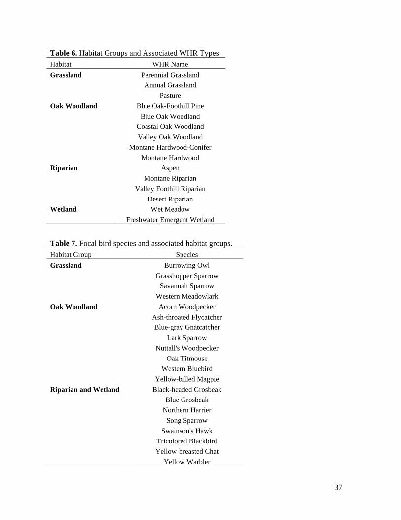
Table 6. Habitat Groups and Associated WHR Types Habitat WHR Name Grassland Perennial Grassland Annual Grassland Pasture Oak Woodland Blue Oak-Foothill Pine Blue Oak Woodland Coastal Oak Woodland Valley Oak Woodland Montane Hardwood-Conifer Montane Hardwood Riparian Aspen Montane Riparian Valley Foothill Riparian Desert Riparian Wetland Wet Meadow Freshwater Emergent Wetland
Table 7. Focal bird species and associated habitat groups. Habitat Group Species Grassland Burrowing Owl Grasshopper Sparrow Savannah Sparrow Western Meadowlark Oak Woodland Acorn Woodpecker Ash-throated Flycatcher Blue-gray Gnatcatcher Lark Sparrow Nuttall's Woodpecker Oak Titmouse Western Bluebird Yellow-billed Magpie Riparian and Wetland Black-headed Grosbeak Blue Grosbeak Northern Harrier Song Sparrow Swainson's Hawk Tricolored Blackbird Yellow-breasted Chat Yellow Warbler
37
38
RESULTS
Current density (Table 8) and potential density (Table 9) estimates for 12 species by
hydrological unit (basin) are presented below. Variation by unit may reflect differences in
sample size, bird distribution, habitat suitability and quality, and intrinsic variation in bird
habitat selection.
Current population estimates from a specific area can be derived from these densities
by multiplying appropriate estimates (birds per hectare) by the area of available habitat to be
enhanced or restored. Population targets may be derived by multiplying the target density by
the amount of area to be restored or enhanced. This process was used to derive population
estimates for riparian focal species in the Central Valley Joint Venture's current
implementation plan (CVJV 2006).
On the website (http://data.prbo.org/cadc/tools/lip/), current and potential density
estimates are also presented at the site level, thus increasing the applicability of these
estimates for individual projects.
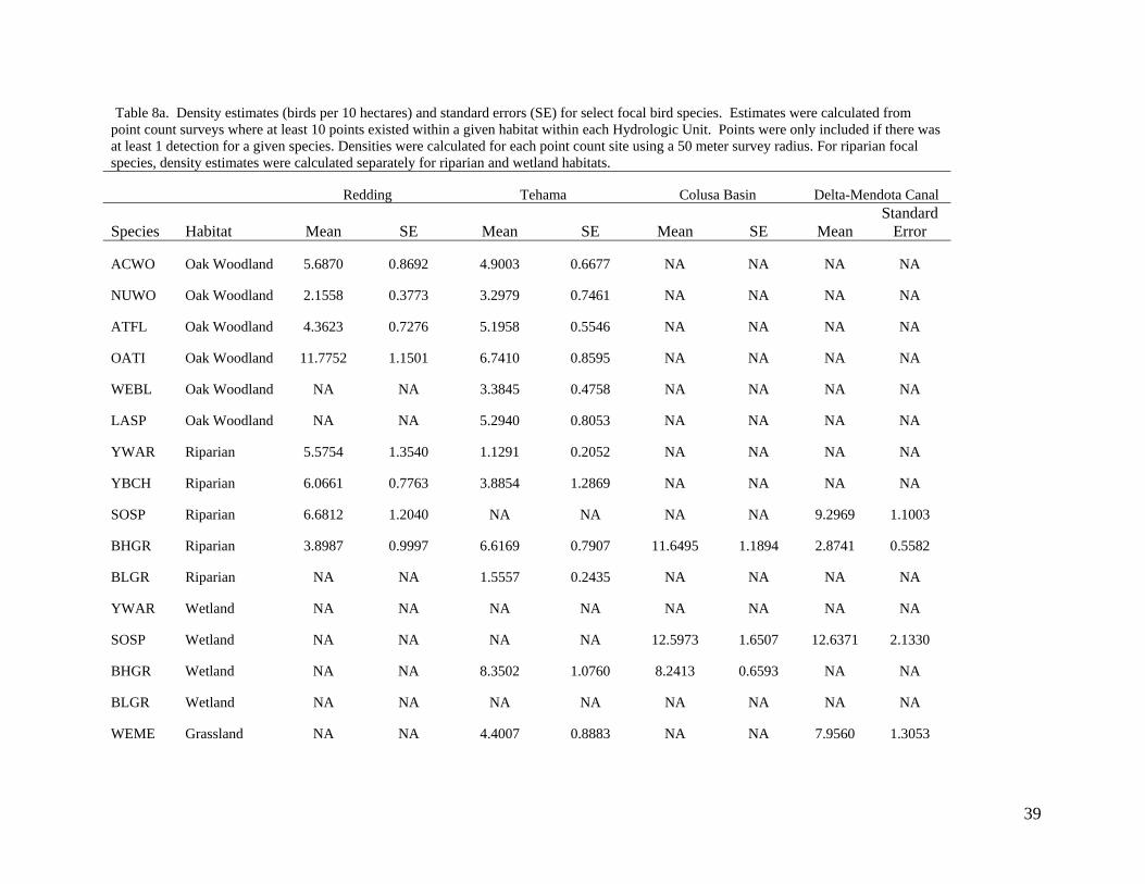
Table 8a. Density estimates (birds per 10 hectares) and standard errors (SE) for select focal bird species. Estimates were calculated from point count surveys where at least 10 points existed within a given habitat within each Hydrologic Unit. Points were only included if there was at least 1 detection for a given species. Densities were calculated for each point count site using a 50 meter survey radius. For riparian focal species, density estimates were calculated separately for riparian and wetland habitats.
Redding Tehama Colusa Basin Delta-Mendota Canal
Species Habitat Mean SE Mean SE Mean SE MeanStandard
Error
ACWO Oak Woodland 5.6870 0.8692 4.9003 0.6677 NA NA NA NA
NUWO
Oak Woodland 2.1558 0.3773 3.2979 0.7461 NA NA NA NA
ATFL Oak Woodland 4.3623 0.7276 5.1958 0.5546 NA NA NA NA
OATI Oak Woodland 11.7752 1.1501 6.7410 0.8595 NA NA NA NA
WEBL Oak Woodland NA NA 3.3845 0.4758 NA NA NA NA
LASP Oak Woodland NA NA 5.2940 0.8053 NA NA NA NA
YWAR Riparian 5.5754 1.3540 1.1291 0.2052 NA NA NA NA
YBCH Riparian 6.0661 0.7763 3.8854 1.2869 NA NA NA NA
SOSP Riparian 6.6812 1.2040 NA NA NA NA 9.2969 1.1003
BHGR Riparian 3.8987 0.9997 6.6169 0.7907 11.6495 1.1894 2.8741 0.5582
BLGR Riparian NA NA 1.5557 0.2435 NA NA NA NA
YWAR Wetland NA NA NA NA NA NA NA NA
SOSP Wetland NA NA NA NA 12.5973 1.6507 12.6371 2.1330
BHGR Wetland NA NA 8.3502 1.0760 8.2413 0.6593 NA NA
BLGR Wetland NA NA NA NA NA NA NA NA
WEME Grassland NA NA 4.4007 0.8883 NA NA 7.9560 1.3053
39

40
Table 8b. Density estimates (birds per 10 hectares) and standard errors (SE) for select focal bird species. Estimates were calculated from point count surveys where at least 10 points existed within a given habitat within each Hydrologic Unit. Points were only included if there was at least 1 detection for a given species. Densities were calculated for each point count site using a 50 meter survey radius. For riparian focal species, density estimates were calculated separately for riparian and wetland habitats.
North Valley Floor San Joaquin Delta San Joaquin Valley
Floor South Valley Floor
Species Habitat Mean SE Mean SE Mean SE Mean SE
ACWO Oak Woodland NA NA NA NA NA NA NA NA
NUWO Oak Woodland
NA NA NA NA 4.5382 0.5115 NA NA
ATFL Oak Woodland NA NA NA NA 6.7675 1.2514 NA NA
OATI Oak Woodland NA NA NA NA 8.2618 1.5888 NA NA
WEBL Oak Woodland NA NA NA NA NA NA NA NA
LASP Oak Woodland NA NA NA NA NA NA NA NA
YWAR Riparian NA NA NA NA NA NA NA NA
YBCH Riparian NA NA NA NA NA NA NA NA
SOSP Riparian NA NA NA NA 7.8230 0.9048 NA NA
BHGR Riparian NA NA NA NA 4.3524 0.7186 NA NA
BLGR Riparian NA NA NA NA NA NA NA NA
YWAR Wetland NA NA 0.9073 0.1569 NA NA NA NA
SOSP Wetland NA NA 17.9444 2.9737 NA NA 19.9768 3.5730
BHGR Wetland NA NA 3.1857 0.6859 NA NA NA NA
BLGR Wetland NA NA 1.8203 0.4049 NA NA NA NA
WEME Grassland NA NA NA NA NA NA NA NA
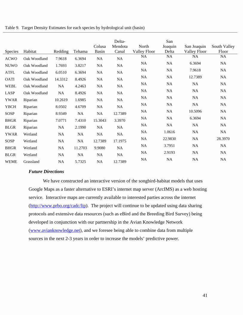
Table 9. Target Density Estimates for each species by hydrological unit (basin)
Species Habitat Redding Tehama Colusa Basin
Delta-Mendota
Canal North
Valley Floor
San Joaquin Delta
San Joaquin Valley Floor
South Valley Floor
ACWO Oak Woodland 7.9618 6.3694 NA NA NA NA NA NA
NUWO Oak Woodland 1.7693 3.8217 NA NA NA NA 6.3694 NA
ATFL Oak Woodland 6.0510 6.3694 NA NA NA NA 7.9618 NA
OATI Oak Woodland 14.3312 8.4926 NA NA NA NA 12.7389 NA
WEBL Oak Woodland NA 4.2463 NA NA NA NA NA NA
LASP Oak Woodland NA 8.4926 NA NA NA NA NA NA
YWAR Riparian 10.2619 1.6985 NA NA NA NA NA NA
YBCH Riparian 8.0502 4.6709 NA NA NA NA NA NA
SOSP Riparian 8.9349 NA NA 12.7389 NA NA 10.5096 NA
BHGR Riparian 7.0771 7.4310 15.3043 3.3970 NA NA 6.3694 NA
BLGR Riparian NA 2.1990 NA NA NA NA NA NA
YWAR Wetland NA NA NA NA NA 1.0616 NA NA
SOSP Wetland NA NA 12.7389 17.1975 NA 22.9830 NA 28.3970
BHGR Wetland NA 11.2703 9.9080 NA NA 3.7951 NA NA
BLGR Wetland NA NA NA NA NA 2.9193 NA NA
WEME Grassland NA 5.7325 NA 12.7389 NA NA NA NA
Google Maps as a faster alternative to ESRI’s internet map server (ArcIMS) as a web hosting
service. Interactive maps are currently available to interested parties across the internet
(http://www.prbo.org/cadc/lip). The project will continue to be updated using data sharing
protocols and extensive data resources (such as eBird and the Breeding Bird Survey) being
developed in conjunction with our partnership in the Avian Knowledge Network
(www.avianknowledge.net), and we foresee being able to combine data from multiple
sources in the next 2-3 years in order to increase the models’ predictive power.
Future Directions
We have constructed an interactive version of the songbird-habitat models that uses
41
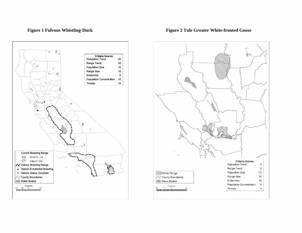
Figure 1 Fulvous Whistling-Duck Figure 2 Tule Greater White-fronted Goose

43
Figure 3 Redhead Figure 4 American White Pelican
44
Figure 5 Least Bittern Figure 6 Snowy Plover
45
Figure 7 Black Tern Figure 8 Modesto Song Sparrow
46
Figure 9 Yellow-headed Blackbird Figure 10 Northern Harrier
47
Figure 11 Lesser Sandhill Crane Figure 12 Short-eared Owl
48
Figure 13 Tricolored Blackbird Figure 14 Mountain Plover
49
Figure 15 Burrowing Owl Figure 16 Oregon Vesper Sparrow
50
Figure 17 Grasshopper Sparrow Figure 18 Yellow-breasted Chat
51
Figure 19 Yellow Warbler Figure 20 Long-eared Owl
52
Figure 21 Purple Martin Figure 22 Loggerhead Shrike
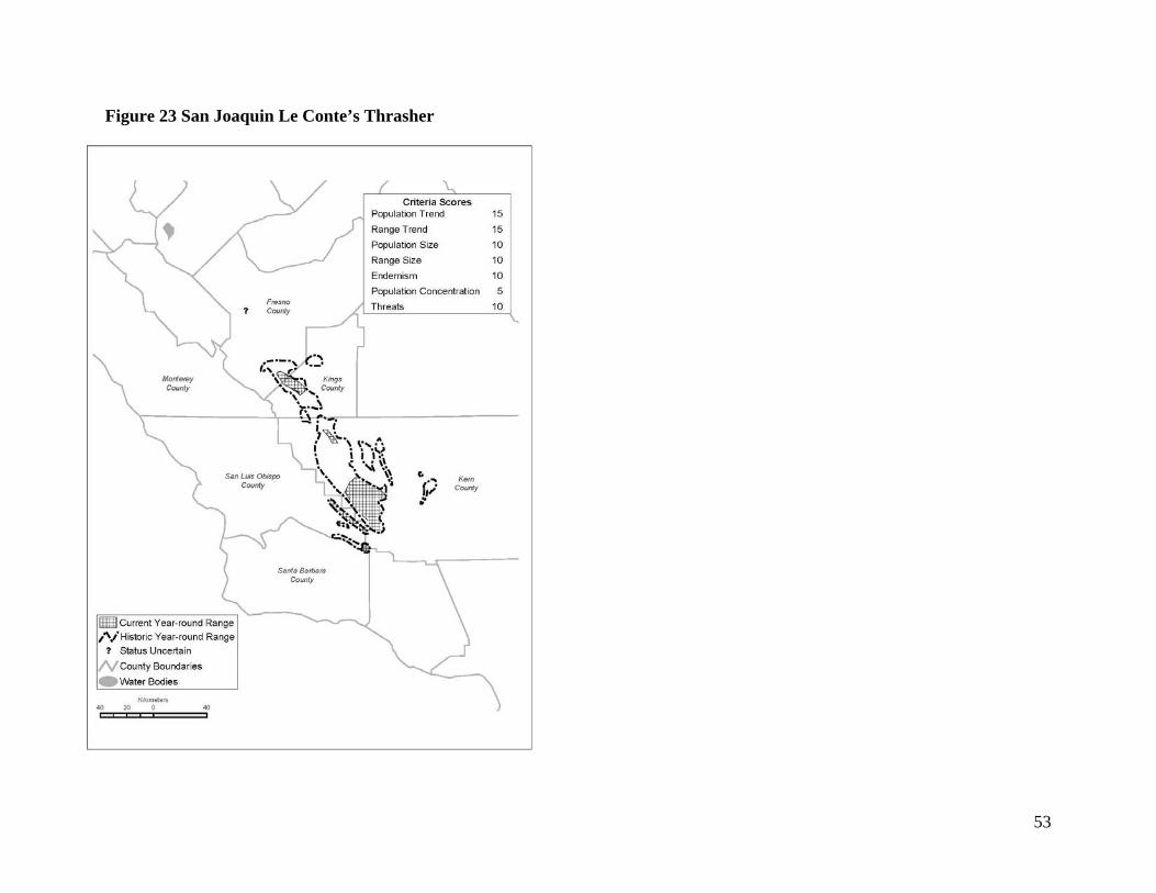
Figure 23 San Joaquin Le Conte’s Thrasher
53

Figure 24 Acorn Woodpecker Figure 25 Ash-throated Flycatcher
54
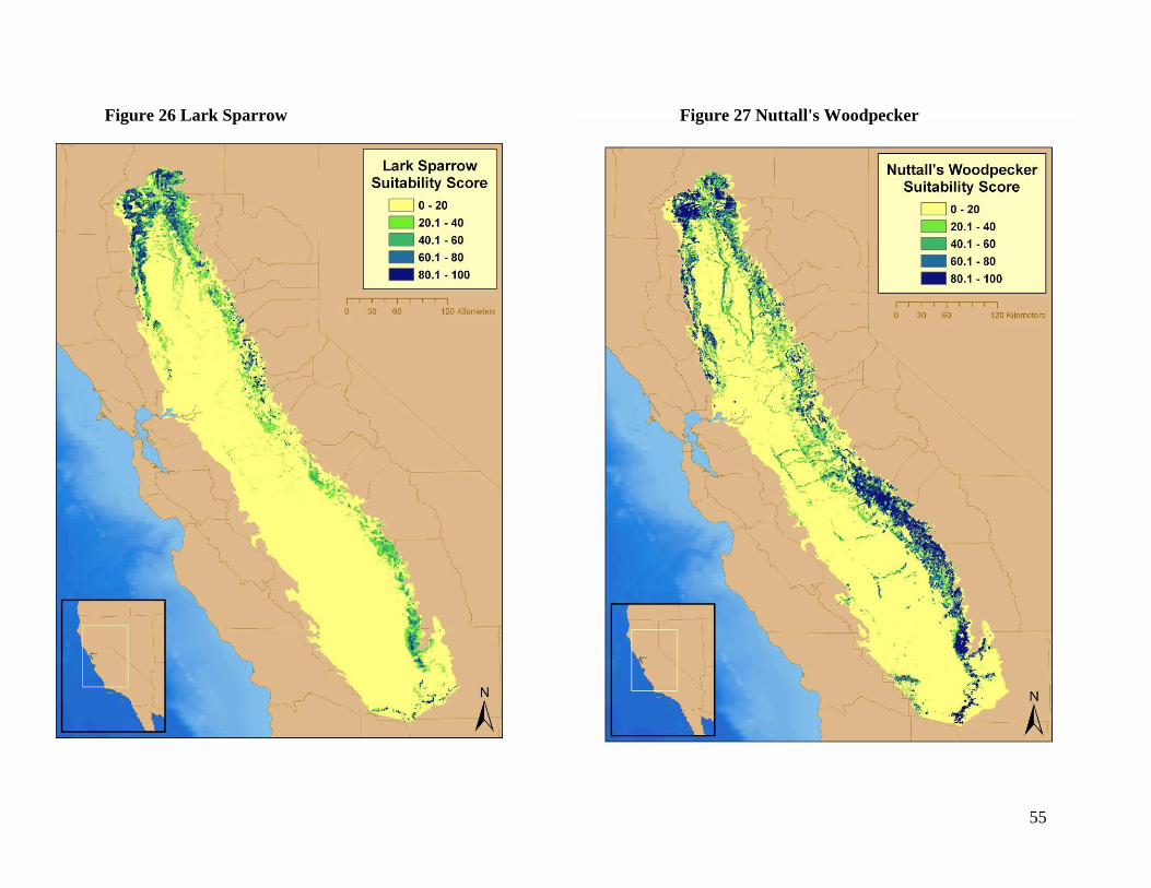
Figure 26 Lark Sparrow Figure 27 Nuttall's Woodpecker
55

Figure 28 Oak Titmouse Figure 29 Western Bluebird
56
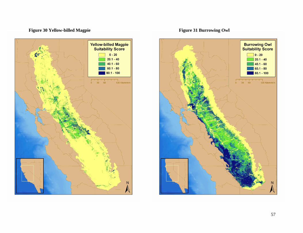
Figure 30 Yellow-billed Magpie Figure 31 Burrowing Owl
57
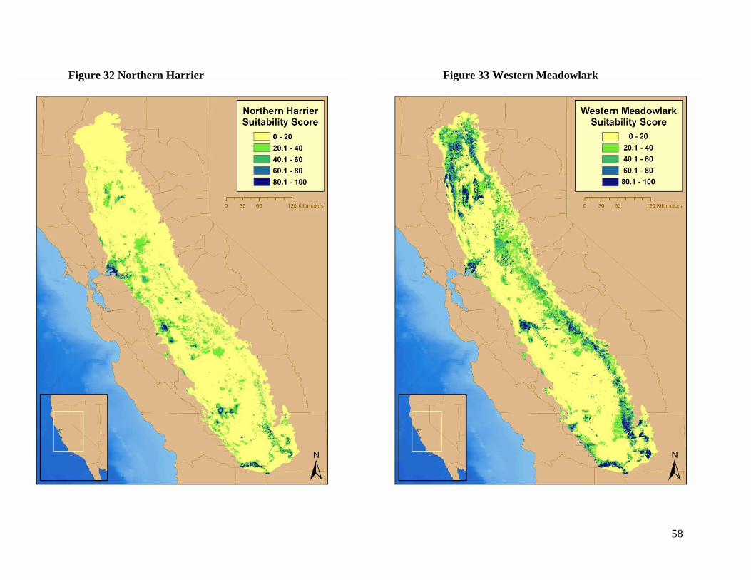
Figure 32 Northern Harrier Figure 33 Western Meadowlark
58
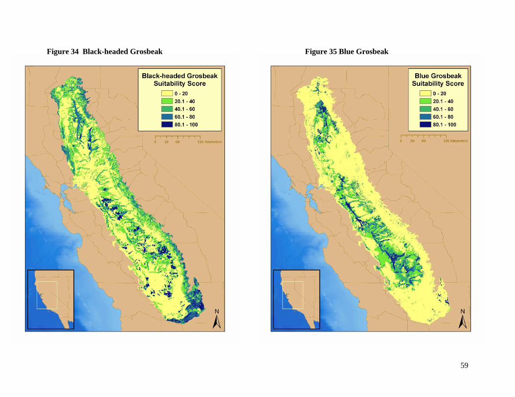
Figure 34 Black-headed Grosbeak Figure 35 Blue Grosbeak
59

Figure 36 Common Yellowthroat Figure 37 Song Sparrow
60

Figure 38 Spotted Towhee Figure 39 Swainson's Hawk
61
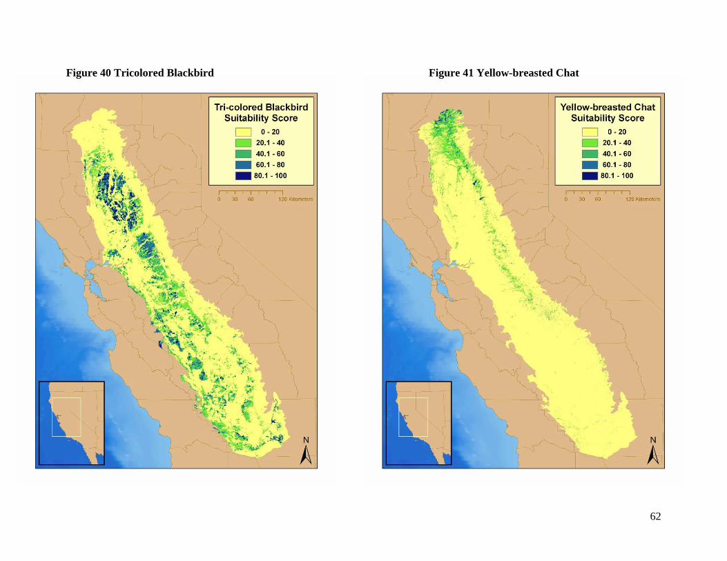
Figure 40 Tricolored Blackbird Figure 41 Yellow-breasted Chat
62

Figure 42 Yellow Warbler Figure 43 Bird Species of Special Concern
(BSSC)
63
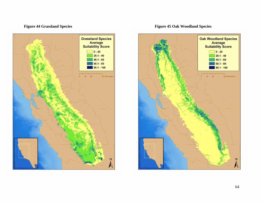
Figure 44 Grassland Species Figure 45 Oak Woodland Species
64

65
Figure 46 Riparian Species Figure 47 PRBO Point Count Locations

LITERATURE CITED
Abbitt, R. J. F., Scott, M. J., and Wilcove, D. S. 2000. The geography of vulnerability:
Incorporating species geography and human development patterns into conservation
planning. Biol. Conserv. 96:169-175.
American Farmland Trust. 1995. Alternatives for future urban growth in California's
Central Valley: The bottom line for agriculture and taxpayers. Am. Farmland Trust,
Washington, D.C.
Aspinall, R., and Veitch, N. 1993. Habitat mapping from satellite imagery and wildlife
survey data using a Bayesian modeling procedure in a GIS. Photoprogramm Eng
Remote Sens. 59:537-543.
Bean, M. J. 2000. Strategies for biodiversity protection, in Precious Heritage: The Status of
Biodiversity in the United States, Chapter 9, pp. 255-273 (B. A. Stein, L. S. Kutner,
and J. S. Adams, eds.). Oxford Univ. Press, New York.
California Department Fish and Game. 1992. Bird species of special concern. Unpublished
list, July 1992, Calif. Dept. Fish & Game, 1416 Ninth St., Sacramento, CA 95814.
California Partners in Flight (B. Allen, lead author). 2000. The draft grassland bird
conservation plan: A strategy for protecting and managing grassland habitats and
associated birds in California. Version 1.0. Point Reyes Bird Observatory, 4990
Shoreline Highway 1, Stinson Beach, CA 94970 (www.prbo.org/calpif/plans.html).
California Partners in Flight (S. Zack, lead author). 2002. The oak woodland bird
conservation plan: A strategy for protecting and managing oak woodland habitats and
associated birds in California. Version 2.0. Point Reyes Bird Observatory, 4990
Shoreline Highway 1, Stinson Beach, CA 94970 (www.prbo.org/calpif/plans.html).
Chase, M K. and G. R. Geupel. 2005. The use of avian focal species for conservation
planning in California. In Proceedings of the Third International Partners in Flight
conference, C.J. Ralph and T.D. Rich eds. USDA Forest Service Gen. Tech. Report
PSW-GTR-191
Central Valley Joint Venture (CVJV). 2006. Central Valley Joint Venture Implementation
Plan – Conserving Bird Habitat. U.S. Fish and Wildlife Service, Sacramento, CA.
66

Dahl, T. E., Johnson, C. E., and Frayer, W. E. 1991. Status and trends of wetlands in the
conterminous United States, mid-1970’s to mid-1980’s. U.S. Dept. Interior, Fish &
Wildl. Serv., Washington, D.C.
Debinski, D. M., and Holt, R. D. 2000. A survey and overview of habitat fragmentation
experiments. Conserv. Biol. 14:342-355.
Elith, J., C. H. Graham, R. P. Anderson, M. Dudik, S. Ferrier, A. Guisan, R. J. Hijmans, F.
Huettmann, J. R. Leathwick, A. Lehmann, J. Li, L. G. Lohmann, B. A. Loiselle, G.
Manion, C. Moritz, M. Nakamura, Y. Nakazawa, J. McC. M. Overton, A. Townsend
Peterson, S. J. Phillips, K. Richardson, R. Scachetti-Pereira, R. E. Schapire, J.
Soberon, S. Williams, M. S. Wisz, and N. E. Zimmermann. 2006. Novel methods
improve prediction of species' distributions from occurrence data. Ecography 29:129-
151.
ESRI. 2006. ArcGIS 9.2. Environmental Systems Research Institute. Redlands, CA.
Fielding, A.H., and J.F. Bell, 1997. A review of methods for the assessment of prediction
errors in conservation presence/absence models. Environ Conserv 24:38-49.
Gardali, T., A. L. Holmes, S. L. Small, N. Nur, G. R. Geupel and G. H. Golet. 2006.
Abundance patterns of landbirds in restored and remnant riparian forests on the
Sacramento River, California, U.S.A. Restoration Ecology 14: 391-403.
Garrison, B.A. 1998. Bank Swallow (Riparia riparia). In The Riparian Bird Conservation
Plan: a strategy for reversing the decline of riparian-associated birds in California.
California Partners in Flight. http://prbo.org/calpif/htmldocs/riparian_v-2.html.
Garrison, B. A., J. M. Humphrey, and S. A. Laymon. 1987. Bank Swallow distribution and
nesting ecology on the Sacramento River, California. West. Birds 18:71-76.
Guisan, A., and N.E. Zimmermann, 2000. Predictive habitat distribution models in ecology.
Ecol Model 135:147-186.
Hastie, T. J., and R. J. Tibshirani. 1990. Generalized Additive Models. Chapman & Hall,
London.
Hernandez, P. A., C. H. Graham, L. L. Master, and D. L. Albert. 2006. The effect of sample
size and species characteristics on performance of different species distribution
modeling methods. Ecography 29:773-785.
67
Hickey, C., Shuford, W. D., Page, G. W., and Warnock, S. 2003. The Southern Pacific
Shorebird Conservation Plan: A strategy for supporting California’s Central Valley
and coastal shorebird populations. Version 1.1. PRBO Conservation Science, 4990
Shoreline Highway 1, Stinson Beach, CA (www.prbo.org/shorebirdconservation).
IUCN. 2006. 2006 IUCN Red List of Threatened Species (www.iucnredlist.org).
Ivey, G.L. 2005. Sandhill Crane objectives and conservation strategies. Unpublished.
Report provided to the Central Valley Joint Venture. 8 pp.
Ivey, G.L. and C.P. Herziger. 2003. Sandhill Crane Monitoring at Staten Island, San
Joaquin County, California, 2002-03. Unpublished report. The Nature Conservancy,
Galt, California. http://www.consumnes.org/staten-cranes.pdf.
Kushlan, J. A., Steinkamp, M. J., Parsons, K., Capp, J., Acosta Cruz, M., Coulter, M.,
Davidson, I., Dickson, L., Edelson, N., Elliot, R., Erwin, R. M., Hatch, S., Kress, S.,
Milko, R., Miller, S., Mills, K., Paul, R., Phillips, R., Saliva, J. E., Sydeman, B.,
Trapp, J., Wheeler, J., and Wohl, K. 2002. Waterbird conservation for the Americas:
The North American waterbird conservation plan, version 1. Waterbirds for the
Americas Initiative, Washington, D.C.
Laymon, S.A. 1998. Yellow-billed Cuckoo (Coccycus americanus). In The Riparian Bird
Conservation Plan: a strategy for reversing the decline of riparian-associated birds in
California. California Partners in Flight. http://prbo.org/calpif/htmldocs/riparian_v-
2.html.
Lindenmayer, D.B., H.A. Nix, J.P. McMahon, M.F. Hutchinson, and M.T. Tanton, 1991. The
conservation of Leadbeater's possum, Gymnobelideus leadbeateri (McCoy): a case
study of the use of bioclimatic modelling. J. Biogeogr. 18:371-383.
McGarigal, K., and B. J. Marks. 1995. FRAGSTATS: spatial pattern analysis program for
quantifying landscape structure. USDA For. Serv. Gen. Tech. Rep. PNW-351.
(http://www.umass.edu/landeco/research/fragstats/fragstats.html).
North American Cowbird Advisory Council. 2003. Website of the North American
Cowbird Advisory Council (http://cowbird.lscf.ucsb.edu/).
North American Waterfowl Management Plan, Plan Committee. 2004. North American
Waterfowl Management Plan 2004. Strategic Guidance: Strengthening the Biological
68

Foundation. Canadian Wildlife Service, U.S. Fish and Wildlife Service, Secretaria de
Medio Ambiente y Recursos Naturales.
Pashley D. and G. R. Geupel 2003. The California Way. Science guides California’s bird
conservation efforts. Bird Conservation 21:8-9.
Phillips, S. J., R. P. Anderson, and R. E. Schapire. 2006. Maximum entropy modeling of
species geographic distributions. Ecological Applications 190:231-259.
Pereira, J.M.C., and R.M. Itami, 1991. GIS-based habitat modelling using logistic multiple
regression: a study of the Mt. Graham Red Squirrel. Photo Eng Rem Sens 57:1475-
1486.
Peters, M. 2000. Reintroduction of Fulvous Whistling-Ducks (Dendrocygna bicolor) to the
San Joaquin Valley, California. Unpublished draft project proposal, dated 28
November 2000, prepared for the San Luis NWR Complex, Los Banos, CA.
Rich, T. D., Beardmore, C. J., Berlanga, H., Blancher, P. J., Bradstreet, M. S. W., Butcher, G.
S., Demarest, D. W., Dunn, E. H., Hunter, W. C., Iñigo-Elias, E. E., Kennedy, J. A.,
Martell, A. M., Panjabi, A. O., Pashley, D. N., Rosenberg, K. V., Rustay, C. M.,
Wendt, J. S., and Will T. C. 2004. Partners in Flight North American Landbird
Conservation Plan (Version: March 2005). Cornell Lab of Ornithology. Ithaca, NY.
(www.partnersinflight.org/cont_plan/)
Richter, B. D., and Richter, H. E. 2000. Prescribing flood regimes to sustain riparian
ecosystems along meandering rivers. Conserv. Biol. 14:1467-1478
RHJV (Riparian Habitat Joint Venture). 2000. Version 1.0. The riparian bird conservation
plan: A strategy for reversing the decline of riparian-associated birds in California.
Calif. Partners in Flight (http://www.prbo.org/CPIF/Riparian/Riparian.html).
Riparian Habitat Joint Venture. 2004. Version 2.0. The riparian bird conservation plan: A
strategy for reversing the decline of riparian-associated birds in California. Calif.
Partners in Flight (www.prbo.org/calpif/plans.html).
Rosenberg, K. V., Ohmart, R. D., Hunter, W. C., and Anderson, B. W. 1991. Birds of the
Lower Colorado River Valley. Univ. Arizona Press, Tucson.
Saunders, D. A., Hobbs, R. J., and Margules, C. R. 1991. Biological consequences of
ecosystem fragmentation: A review. Biol. Conserv. 5:18-32.
69
Schlorff, R. W. 1992. Recovery plan: Bank Swallow (Riparia riparia). State of Calif.
Resources Agency, Dept. of Fish and Game, Sacramento, CA.
Shuford, W.D. and T. Gardali. In press. California Bird Species of Special Concern 2006.
California Department of Fish and Game, Sacramento, CA. Western Birds.
Monograph.
Shuford, W. D., Humphrey, J. M., and Nur, N. 2001. Breeding status of the Black Tern in
California. W. Birds 32:189-217.
Smith, J. N. M. 1999. The basis for cowbird management: Host selection, impacts on hosts,
and criteria for taking management action. Studies Avian Biol. 18:104-108.
Sorensen, A. A., Greene, R. P., and Russ, K. 1997. Farming on the edge. Am. Farmland
Trust, Center for Agriculture in the Environment, Northern Illinois Univ., DeKalb,
IL.
Squires, J. R., Hayward, G. D., and Gore, J. F. 1998. The role of sensitive species in avian
conservation, in Avian Conservation: Research and Management (J. M. Marzluff and
R. Sallabanks, eds.), pp.141-154. Island Press, Washington, DC.
Stein, B. A. 2002. States of the union: Ranking America’s biodiversity. NatureServe,
Arlington, VA (www.natureserve.org/publications/statesUnion.jsp).
Stein, B. A., Kutner, L. S., Hammerson, G. A., Master, L. L., and Morse, L. E. 2000. State
of the states: geographic patterns of diversity, rarity, and endemism, in Precious
Heritage: The Status of Biodiversity in the United States, Chapter 5, pp. 119-157 (B.
A. Stein, L. S. Kutner, and J. S. Adams, eds.). Oxford Univ. Press, New York.
Swets, J. 1988. Measuring the accuracy of diagnostic systems. Science 240:1285-1293.
Tricolored Blackbird Working Group (TBWG). 2007. Conservation plan for the Tricolored
Blackbird (Agelaius tricolor). Edited by Susan Kester, Sustainable Conservation, San
Francisco (www.suscon.org/download/TricolorConservationPlanandMOA.pdf).
U.S. Fish and Wildlife Service. 2002. Birds of Conservation Concern 2002. U.S. Fish &
Wildl. Serv., Div. Migratory Bird Mgmt., Arlington, VA
(http://migratorybirds.fws.gov/reports/bcc2002.pdf).
Wilcove, D. S., Rothstein, D., Dubow, J., Phillips, A., and Losos, E. 1998. Quantifying
threats to imperiled species in the United States: Assessing the relative importance of
70
habitat destruction, alien species, pollution, overexploitation, and disease.
BioScience 48:607-615.
Wilcove, D. S., Rothstein, D., Dubow, J., Phillips, A., and Losos, E. 2000. Leading threats
to biodiversity: What’s imperiling U.S. species, in Precious Heritage: The Status of
Biodiversity in the United States, Chapter 8, pp. 239-254 (B. A. Stein, L. S. Kutner,
and J. S. Adams, eds.). Oxford Univ. Press, New York.
Woodbridge, B. 1998. Swainson’s Hawk (Buteo swainsoni). In The Riparian Bird
Conservation Plan: a strategy for reversing the decline of riparian-associated birds in
California. California Partners in Flight
(http://www.prbo.org/calpif/htmldocs/riparian_v-2.html).
71
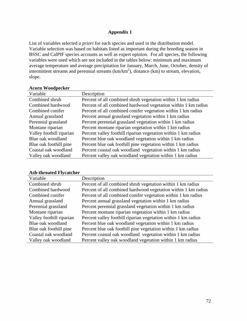
Appendix 1 List of variables selected a priori for each species and used in the distribution model. Variable selection was based on habitats listed as important during the breeding season in BSSC and CalPIF species accounts as well as expert opinion. For all species, the following variables were used which are not included in the tables below: minimum and maximum average temperature and average precipitation for January, March, June, October, density of intermittent streams and perennial streams (km/km2), distance (km) to stream, elevation, slope. Acorn Woodpecker Variable Description Combined shrub Percent of all combined shrub vegetation within 1 km radius Combined hardwood Percent of all combined hardwood vegetation within 1 km radius Combined conifer Percent of all combined conifer vegetation within 1 km radius Annual grassland Percent annual grassland vegetation within 1 km radius Perennial grassland Percent perennial grassland vegetation within 1 km radius Montane riparian Percent montane riparian vegetation within 1 km radius Valley foothill riparian Percent valley foothill riparian vegetation within 1 km radius Blue oak woodland Percent blue oak woodland vegetation within 1 km radius Blue oak foothill pine Percent blue oak foothill pine vegetation within 1 km radius Coastal oak woodland Percent coastal oak woodland vegetation within 1 km radius Valley oak woodland Percent valley oak woodland vegetation within 1 km radius Ash-throated Flycatcher Variable Description Combined shrub Percent of all combined shrub vegetation within 1 km radius Combined hardwood Percent of all combined hardwood vegetation within 1 km radius Combined conifer Percent of all combined conifer vegetation within 1 km radius Annual grassland Percent annual grassland vegetation within 1 km radius Perennial grassland Percent perennial grassland vegetation within 1 km radius Montane riparian Percent montane riparian vegetation within 1 km radius Valley foothill riparian Percent valley foothill riparian vegetation within 1 km radius Blue oak woodland Percent blue oak woodland vegetation within 1 km radius Blue oak foothill pine Percent blue oak foothill pine vegetation within 1 km radius Coastal oak woodland Percent coastal oak woodland vegetation within 1 km radius Valley oak woodland Percent valley oak woodland vegetation within 1 km radius
72
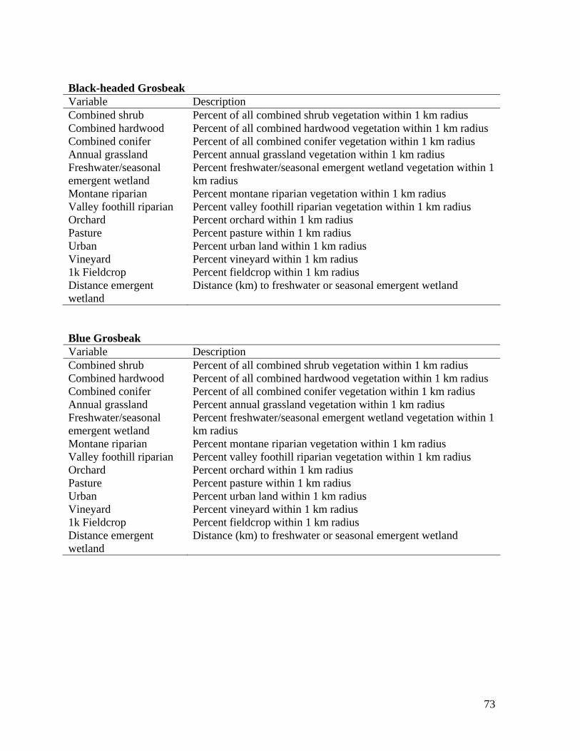
Black-headed Grosbeak Variable Description Combined shrub Percent of all combined shrub vegetation within 1 km radius Combined hardwood Percent of all combined hardwood vegetation within 1 km radius Combined conifer Percent of all combined conifer vegetation within 1 km radius Annual grassland Percent annual grassland vegetation within 1 km radius Freshwater/seasonal emergent wetland
Percent freshwater/seasonal emergent wetland vegetation within 1 km radius
Montane riparian Percent montane riparian vegetation within 1 km radius Valley foothill riparian Percent valley foothill riparian vegetation within 1 km radius Orchard Percent orchard within 1 km radius Pasture Percent pasture within 1 km radius Urban Percent urban land within 1 km radius Vineyard Percent vineyard within 1 km radius 1k Fieldcrop Percent fieldcrop within 1 km radius Distance emergent wetland
Distance (km) to freshwater or seasonal emergent wetland
Blue Grosbeak Variable Description Combined shrub Percent of all combined shrub vegetation within 1 km radius Combined hardwood Percent of all combined hardwood vegetation within 1 km radius Combined conifer Percent of all combined conifer vegetation within 1 km radius Annual grassland Percent annual grassland vegetation within 1 km radius Freshwater/seasonal emergent wetland
Percent freshwater/seasonal emergent wetland vegetation within 1 km radius
Montane riparian Percent montane riparian vegetation within 1 km radius Valley foothill riparian Percent valley foothill riparian vegetation within 1 km radius Orchard Percent orchard within 1 km radius Pasture Percent pasture within 1 km radius Urban Percent urban land within 1 km radius Vineyard Percent vineyard within 1 km radius 1k Fieldcrop Percent fieldcrop within 1 km radius Distance emergent wetland
Distance (km) to freshwater or seasonal emergent wetland
73
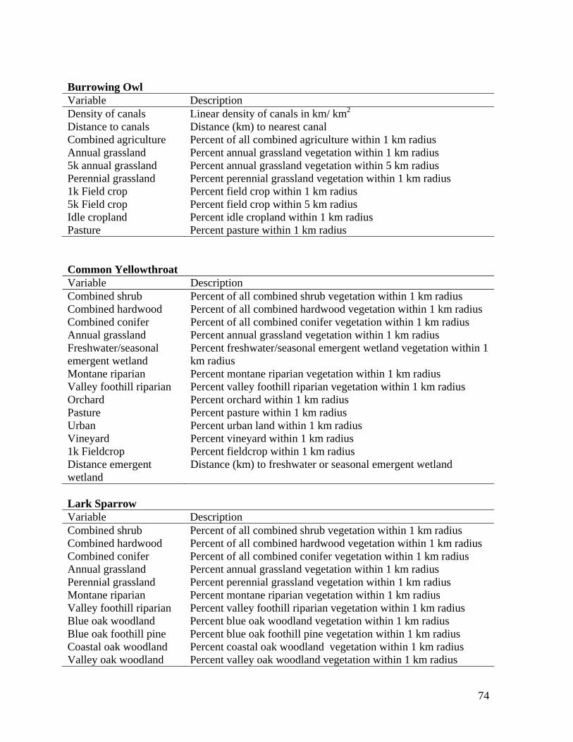
Burrowing Owl Variable Description Density of canals Linear density of canals in km/ km2
Distance to canals Distance (km) to nearest canal Combined agriculture Percent of all combined agriculture within 1 km radius Annual grassland Percent annual grassland vegetation within 1 km radius 5k annual grassland Percent annual grassland vegetation within 5 km radius Perennial grassland Percent perennial grassland vegetation within 1 km radius 1k Field crop Percent field crop within 1 km radius 5k Field crop Percent field crop within 5 km radius Idle cropland Percent idle cropland within 1 km radius Pasture Percent pasture within 1 km radius Common Yellowthroat Variable Description Combined shrub Percent of all combined shrub vegetation within 1 km radius Combined hardwood Percent of all combined hardwood vegetation within 1 km radius Combined conifer Percent of all combined conifer vegetation within 1 km radius Annual grassland Percent annual grassland vegetation within 1 km radius Freshwater/seasonal emergent wetland
Percent freshwater/seasonal emergent wetland vegetation within 1 km radius
Montane riparian Percent montane riparian vegetation within 1 km radius Valley foothill riparian Percent valley foothill riparian vegetation within 1 km radius Orchard Percent orchard within 1 km radius Pasture Percent pasture within 1 km radius Urban Percent urban land within 1 km radius Vineyard Percent vineyard within 1 km radius 1k Fieldcrop Percent fieldcrop within 1 km radius Distance emergent wetland
Distance (km) to freshwater or seasonal emergent wetland
Lark Sparrow Variable Description Combined shrub Percent of all combined shrub vegetation within 1 km radius Combined hardwood Percent of all combined hardwood vegetation within 1 km radius Combined conifer Percent of all combined conifer vegetation within 1 km radius Annual grassland Percent annual grassland vegetation within 1 km radius Perennial grassland Percent perennial grassland vegetation within 1 km radius Montane riparian Percent montane riparian vegetation within 1 km radius Valley foothill riparian Percent valley foothill riparian vegetation within 1 km radius Blue oak woodland Percent blue oak woodland vegetation within 1 km radius Blue oak foothill pine Percent blue oak foothill pine vegetation within 1 km radius Coastal oak woodland Percent coastal oak woodland vegetation within 1 km radius Valley oak woodland Percent valley oak woodland vegetation within 1 km radius
74
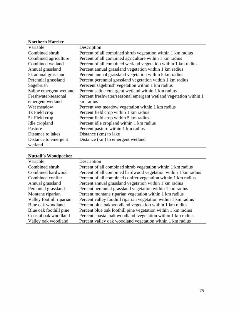
Northern Harrier Variable Description Combined shrub Percent of all combined shrub vegetation within 1 km radius Combined agriculture Percent of all combined agriculture within 1 km radius Combined wetland Percent of all combined wetland vegetation within 1 km radius Annual grassland Percent annual grassland vegetation within 1 km radius 5k annual grassland Percent annual grassland vegetation within 5 km radius Perennial grassland Percent perennial grassland vegetation within 1 km radius Sagebrush Perecent sagebrush vegetation within 1 km radius Saline emergent wetland Percent saline emergent wetland within 1 km radius Freshwater/seasonal emergent wetland
Percent freshwater/seasonal emergent wetland vegetation within 1 km radius
Wet meadow Percent wet meadow vegetation within 1 km radius 1k Field crop Percent field crop within 1 km radius 5k Field crop Percent field crop within 5 km radius Idle cropland Percent idle cropland within 1 km radius Pasture Percent pasture within 1 km radius Distance to lakes Distance (km) to lake Distance to emergent wetland
Distance (km) to emergent wetland
Nuttall’s Woodpecker Variable Description Combined shrub Percent of all combined shrub vegetation within 1 km radius Combined hardwood Percent of all combined hardwood vegetation within 1 km radius Combined conifer Percent of all combined conifer vegetation within 1 km radius Annual grassland Percent annual grassland vegetation within 1 km radius Perennial grassland Percent perennial grassland vegetation within 1 km radius Montane riparian Percent montane riparian vegetation within 1 km radius Valley foothill riparian Percent valley foothill riparian vegetation within 1 km radius Blue oak woodland Percent blue oak woodland vegetation within 1 km radius Blue oak foothill pine Percent blue oak foothill pine vegetation within 1 km radius Coastal oak woodland Percent coastal oak woodland vegetation within 1 km radius Valley oak woodland Percent valley oak woodland vegetation within 1 km radius
75

Oak Titmouse Variable Description Combined shrub Percent of all combined shrub vegetation within 1 km radius Combined hardwood Percent of all combined hardwood vegetation within 1 km radius Combined conifer Percent of all combined conifer vegetation within 1 km radius Annual grassland Percent annual grassland vegetation within 1 km radius Perennial grassland Percent perennial grassland vegetation within 1 km radius Montane riparian Percent montane riparian vegetation within 1 km radius Valley foothill riparian Percent valley foothill riparian vegetation within 1 km radius Blue oak woodland Percent blue oak woodland vegetation within 1 km radius Blue oak foothill pine Percent blue oak foothill pine vegetation within 1 km radius Coastal oak woodland Percent coastal oak woodland vegetation within 1 km radius Valley oak woodland Percent valley oak woodland vegetation within 1 km radius Song Sparrow Variable Description Combined shrub Percent of all combined shrub vegetation within 1 km radius Combined hardwood Percent of all combined hardwood vegetation within 1 km radius Combined conifer Percent of all combined conifer vegetation within 1 km radius Annual grassland Percent annual grassland vegetation within 1 km radius Freshwater/seasonal emergent wetland
Percent freshwater/seasonal emergent wetland vegetation within 1 km radius
Montane riparian Percent montane riparian vegetation within 1 km radius Valley foothill riparian Percent valley foothill riparian vegetation within 1 km radius Orchard Percent orchard within 1 km radius Pasture Percent pasture within 1 km radius Urban Percent urban land within 1 km radius Vineyard Percent vineyard within 1 km radius 1k Fieldcrop Percent fieldcrop within 1 km radius Distance emergent wetland
Distance (km) to freshwater or seasonal emergent wetland
76
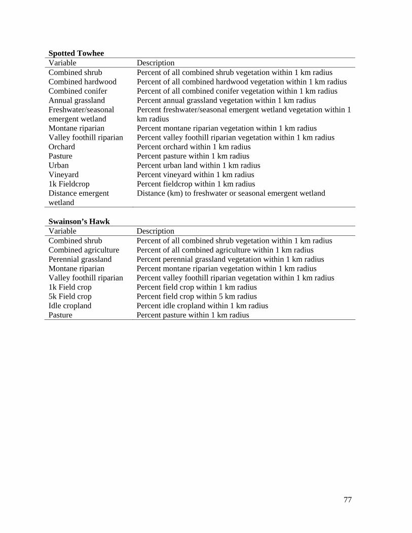
Spotted Towhee Variable Description Combined shrub Percent of all combined shrub vegetation within 1 km radius Combined hardwood Percent of all combined hardwood vegetation within 1 km radius Combined conifer Percent of all combined conifer vegetation within 1 km radius Annual grassland Percent annual grassland vegetation within 1 km radius Freshwater/seasonal emergent wetland
Percent freshwater/seasonal emergent wetland vegetation within 1 km radius
Montane riparian Percent montane riparian vegetation within 1 km radius Valley foothill riparian Percent valley foothill riparian vegetation within 1 km radius Orchard Percent orchard within 1 km radius Pasture Percent pasture within 1 km radius Urban Percent urban land within 1 km radius Vineyard Percent vineyard within 1 km radius 1k Fieldcrop Percent fieldcrop within 1 km radius Distance emergent wetland
Distance (km) to freshwater or seasonal emergent wetland
Swainson’s Hawk Variable Description Combined shrub Percent of all combined shrub vegetation within 1 km radius Combined agriculture Percent of all combined agriculture within 1 km radius Perennial grassland Percent perennial grassland vegetation within 1 km radius Montane riparian Percent montane riparian vegetation within 1 km radius Valley foothill riparian Percent valley foothill riparian vegetation within 1 km radius 1k Field crop Percent field crop within 1 km radius 5k Field crop Percent field crop within 5 km radius Idle cropland Percent idle cropland within 1 km radius Pasture Percent pasture within 1 km radius
77
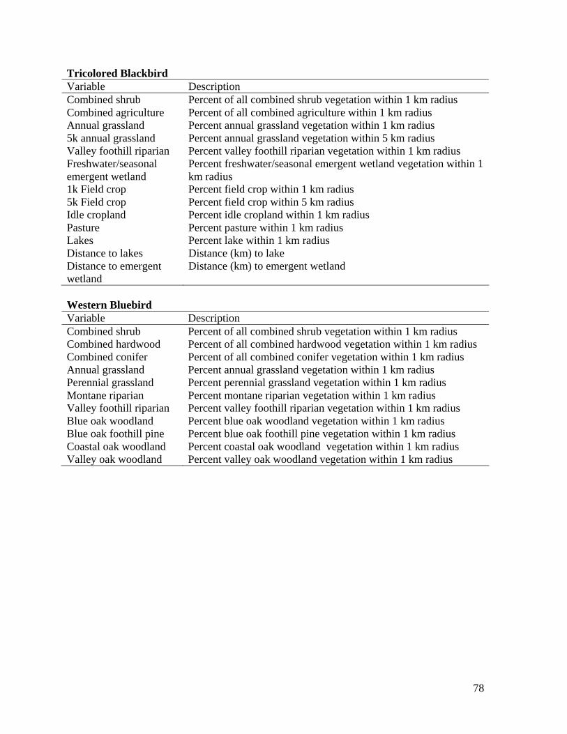
Tricolored Blackbird Variable Description Combined shrub Percent of all combined shrub vegetation within 1 km radius Combined agriculture Percent of all combined agriculture within 1 km radius Annual grassland Percent annual grassland vegetation within 1 km radius 5k annual grassland Percent annual grassland vegetation within 5 km radius Valley foothill riparian Percent valley foothill riparian vegetation within 1 km radius Freshwater/seasonal emergent wetland
Percent freshwater/seasonal emergent wetland vegetation within 1 km radius
1k Field crop Percent field crop within 1 km radius 5k Field crop Percent field crop within 5 km radius Idle cropland Percent idle cropland within 1 km radius Pasture Percent pasture within 1 km radius Lakes Percent lake within 1 km radius Distance to lakes Distance (km) to lake Distance to emergent wetland
Distance (km) to emergent wetland
Western Bluebird Variable Description Combined shrub Percent of all combined shrub vegetation within 1 km radius Combined hardwood Percent of all combined hardwood vegetation within 1 km radius Combined conifer Percent of all combined conifer vegetation within 1 km radius Annual grassland Percent annual grassland vegetation within 1 km radius Perennial grassland Percent perennial grassland vegetation within 1 km radius Montane riparian Percent montane riparian vegetation within 1 km radius Valley foothill riparian Percent valley foothill riparian vegetation within 1 km radius Blue oak woodland Percent blue oak woodland vegetation within 1 km radius Blue oak foothill pine Percent blue oak foothill pine vegetation within 1 km radius Coastal oak woodland Percent coastal oak woodland vegetation within 1 km radius Valley oak woodland Percent valley oak woodland vegetation within 1 km radius
78

Western Meadowlark Variable Description Combined shrub Percent of all combined shrub vegetation within 1 km radius Combined agriculture Percent of all combined agriculture within 1 km radius Combined wetland Percent of all combined wetland vegetation within 1 km radius Annual grassland Percent annual grassland vegetation within 1 km radius Perennial grassland Percent perennial grassland vegetation within 1 km radius Blue oak woodland Percent blue oak woodland vegetation within 1 km radius Coastal oak woodland Percent coastal oak woodland vegetation within 1 km radius Valley oak woodland Percent valley oak woodland vegetation within 1 km radius 1k Field crop Percent field crop within 1 km radius 5k Field crop Percent field crop within 5 km radius Idle cropland Percent idle cropland within 1 km radius Orchards Percent orchards within 1 km radius Pasture Percent pasture within 1 km radius Yellow-breasted Chat Variable Description Combined shrub Percent of all combined shrub vegetation within 1 km radius Combined hardwood Percent of all combined hardwood vegetation within 1 km radius Combined conifer Percent of all combined conifer vegetation within 1 km radius Annual grassland Percent annual grassland vegetation within 1 km radius Freshwater/seasonal emergent wetland
Percent freshwater/seasonal emergent wetland vegetation within 1 km radius
Montane riparian Percent montane riparian vegetation within 1 km radius Valley foothill riparian Percent valley foothill riparian vegetation within 1 km radius Orchard Percent orchard within 1 km radius Pasture Percent pasture within 1 km radius Urban Percent urban land within 1 km radius Vineyard Percent vineyard within 1 km radius 1k Fieldcrop Percent fieldcrop within 1 km radius Distance emergent wetland
Distance (km) to freshwater or seasonal emergent wetland
79

Yellow-billed Magpie Variable Description Combined shrub Percent of all combined shrub vegetation within 1 km radius Combined hardwood Percent of all combined hardwood vegetation within 1 km radius Combined conifer Percent of all combined conifer vegetation within 1 km radius Annual grassland Percent annual grassland vegetation within 1 km radius Perennial grassland Percent perennial grassland vegetation within 1 km radius Montane riparian Percent montane riparian vegetation within 1 km radius Valley foothill riparian Percent valley foothill riparian vegetation within 1 km radius Blue oak woodland Percent blue oak woodland vegetation within 1 km radius Blue oak foothill pine Percent blue oak foothill pine vegetation within 1 km radius Coastal oak woodland Percent coastal oak woodland vegetation within 1 km radius Valley oak woodland Percent valley oak woodland vegetation within 1 km radius Yellow Warbler Variable Description Combined shrub Percent of all combined shrub vegetation within 1 km radius Combined hardwood Percent of all combined hardwood vegetation within 1 km radius Combined conifer Percent of all combined conifer vegetation within 1 km radius Annual grassland Percent annual grassland vegetation within 1 km radius Freshwater/seasonal emergent wetland
Percent freshwater/seasonal emergent wetland vegetation within 1 km radius
Montane riparian Percent montane riparian vegetation within 1 km radius Valley foothill riparian Percent valley foothill riparian vegetation within 1 km radius Orchard Percent orchard within 1 km radius Pasture Percent pasture within 1 km radius Urban Percent urban land within 1 km radius Vineyard Percent vineyard within 1 km radius 1k Fieldcrop Percent fieldcrop within 1 km radius Distance emergent wetland
Distance (km) to freshwater or seasonal emergent wetland
80