Landslide Susceptibility Mapping of Urban Areas: Logistic

RESEARCH Open Access

Landslide Susceptibility Mapping of UrbanAreas: Logistic Regression and SensitivityAnalysis applied to Quito, EcuadorFernando Puente-Sotomayor1,2* , Ahmed Mustafa3 and Jacques Teller1

Abstract

Although the Andean region is one of the most landslide-susceptible areas in the world, limited attention has beendevoted to the topic in this context in terms of research, risk reduction practice, and urban policy. Based on thecollection of landslides data of the Andean city of Quito, Ecuador, this article aims to explore the predictive powerof a binary logistic regression model (LOGIT) to test secondary data and an official multicriteria evaluation model forlandslide susceptibility in this urban area. Cell size resampling scenarios were explored as a parameter, as theinclusion of new “urban” factors. Furthermore, two types of sensitivity analysis (SA), univariate and Monte Carlomethods, were applied to improve the calibration of the LOGIT model. A Kolmogorov–Smirnov (K-S) test wasincluded to measure the classification power of the models. Charts of the three SA methods helped to visualize thesensitivity of factors in the models. The Area Under the Curve (AUC) was a common metric for validation in thisresearch. Among the ten factors included in the model to help explain landslide susceptibility in the context ofQuito, results showed that population and street/road density, as novel “urban factors”, have relevant predictingpower for landslide susceptibility in urban areas when adopting data standardization based on weights assigned byexperts. The LOGIT was validated with an AUC of 0.79. Sensitivity analyses suggested that calibrations of the best-performance reference model would improve its AUC by up to 0.53%. Further experimentation regarding othermethods of data pre-processing and a finer level of disaggregation of input data are suggested. In terms of policydesign, the LOGIT model coefficient values suggest the need for a deep analysis of the impacts of urban features,such as population, road density, building footprint, and floor area, at a household scale, on the generation oflandslide susceptibility in Andean cities such as Quito. This would help improve the zoning for landslide riskreduction, considering the safety, social and economic impacts that this practice may produce.

Keywords: Landslide susceptibility, Quito, LOGIT, Sensitivity analysis, Kolmogorov-Smirnov test, Andean cities, Urbanfactors

© The Author(s). 2021 Open Access This article is licensed under a Creative Commons Attribution 4.0 International License,which permits use, sharing, adaptation, distribution and reproduction in any medium or format, as long as you giveappropriate credit to the original author(s) and the source, provide a link to the Creative Commons licence, and indicate ifchanges were made. The images or other third party material in this article are included in the article's Creative Commonslicence, unless indicated otherwise in a credit line to the material. If material is not included in the article's Creative Commonslicence and your intended use is not permitted by statutory regulation or exceeds the permitted use, you will need to obtainpermission directly from the copyright holder. To view a copy of this licence, visit http://creativecommons.org/licenses/by/4.0/.

* Correspondence: [email protected] Environmental Management and Analysis (LEMA), Urban andEnvironmental Engineering Dept., Liège University, Liège, Belgium2Facultad de Arquitectura y Urbanismo, Universidad Central del Ecuador,Quito, EcuadorFull list of author information is available at the end of the article

Geoenvironmental DisastersPuente-Sotomayor et al. Geoenvironmental Disasters (2021) 8:19 https://doi.org/10.1186/s40677-021-00184-0

http://crossmark.crossref.org/dialog/?doi=10.1186/s40677-021-00184-0&domain=pdf

http://orcid.org/0000-0002-3430-7831

https://orcid.org/0000-0002-1592-6637

https://orcid.org/0000-0003-2498-1838

http://creativecommons.org/licenses/by/4.0/

mailto:[email protected]

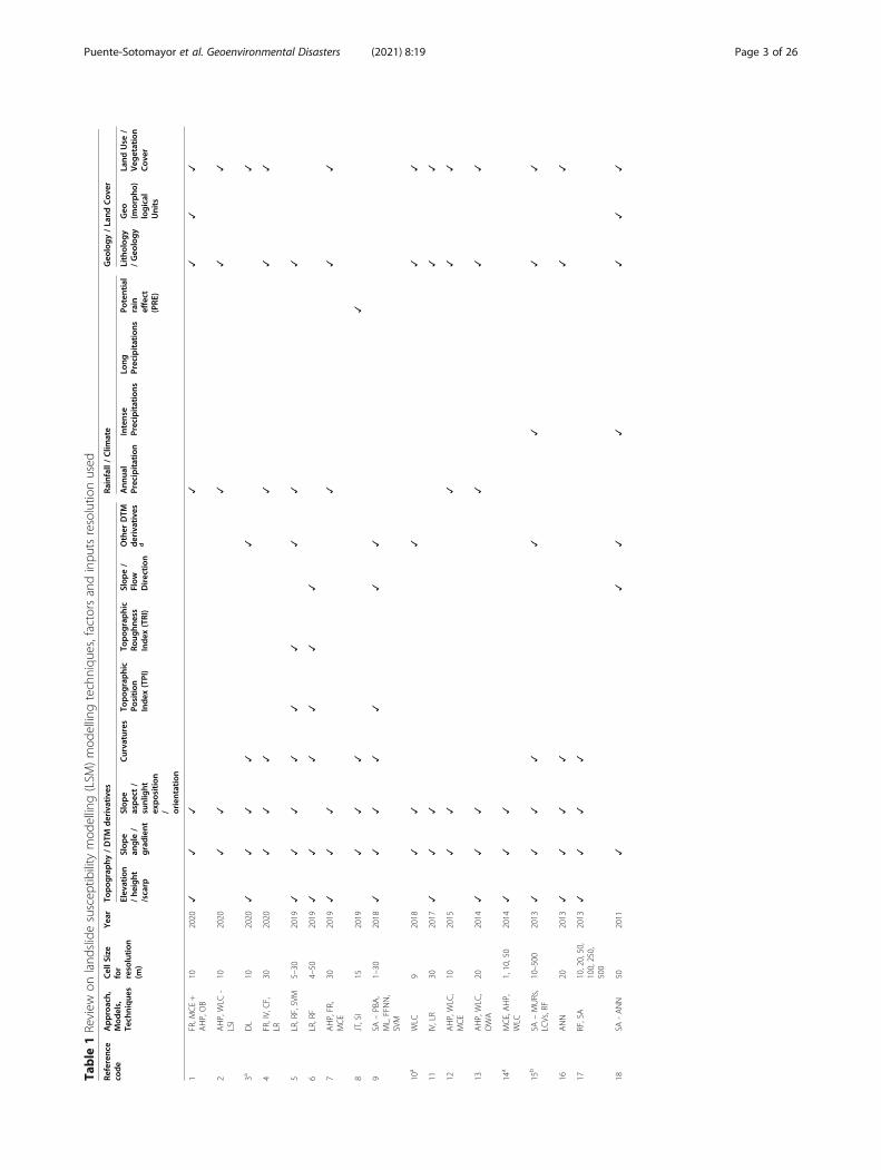
IntroductionUrban landslides in the AndesThe Andes is a sub-region located in western SouthAmerica near the Pacific Ocean, named after the pres-ence of the Andean mountains. The Andean mountainrange is among the cordilleras with the highest eleva-tions in the world and part of the Pacific Ring of Fire, aglobal mountain system characterized by frequent vol-canic eruptions and earthquakes (Blanchard-Boehm2004). The range crosses the territories of Colombia,Ecuador, Perú, Bolivia, Chile, and—with less significancefor human settlements—Argentina and Venezuela. TheAndes orography is of particular concern in terms ofsustainable urban development because it has been sub-ject to significant urbanization processes in recent de-cades, at an average of 20 m2 per minute, particularlyinformal and diverse in typologies (Inostroza 2017). Thisgrowth includes metropolises such as Bogotá, Santiago,and Lima. Other medium-size cities, such as Medellin,Quito, and Cali, and smaller cities, also must be consid-ered in terms of urban population growth. Thisurbanization has been induced by country–city migra-tion and natural growth, for which housing and urbandevelopment—mostly informal and contributing tourban poverty—is a challenge to planning and manage-ment at all governmental levels, which have had to shifttheir policy paradigm (Blanchard-Boehm 2004; vanLindert 2016). Furthermore, cities are subject to urbanrisk in the Andes, where one of the most frequent risks,with high accumulated impact, is landslides.Susceptibility analysis of landslide risk (LRisk) has

been broadly studied in case studies at regional scalesand mostly covering rural areas, often involving naturalconditions and, to a lesser extent, considering anthropicfactors, such as road networks and urban areas. How-ever, urbanization is often treated only as a generic land-use category, without further detail. Against this back-ground, LRisk is one of the main concerns for urban de-velopment in the Andes in light of physical and socialfactors. The geodynamics of this region make it prone tolandslides. This condition is aggravated by climate change,in addition to the extreme events produced by El Niñoclimatic phenomena, which affect diverse locations of theregion with an irregular time cycle. In some of these areas,urbanization has expanded rapidly in recent decades, asmentioned above. Cities in the Andes account for 70% ofthe population and the share of the urban populationcontinues to grow rapidly. Unplanned urbanization isdeveloping without any consideration of LRisks andgovernmental bodies have limited capacities to man-age urban development (Comunidad Andina 2017;D’Ercole et al. 2009; UNISDR 2018). Evidence regard-ing landslide-prone conditions in the region has beenpresented by Kirschbaum and Stanley (2018) and

Sepúlveda and Petley (2015). These studies portraythe concentration of landslide-susceptible areas in theirregular orography of Colombia, Ecuador, and Peru,with hundreds of fatalities. By comparison, fewer fa-talities have occurred in neighboring countries inSouth America, with the exception of Brazil. Accord-ingly, disaster risk management (DRM) should be bet-ter integrated with land-use planning (LUP) forappropriate diagnostics and effective reduction ofrisks related to landslides.

Theoretical backgroundKey definitionsA landslide is defined as: “the downslope movement ofsoil, rock, and organic materials under the effects ofgravity” (Highland and Bobrowsky 2008, p. 4). Its typesinclude slides, falls, topples, flows, and lateral spreads,and combinations of these, whose causes can be geo-logical, morphological, or anthropic (shaping of built ornatural landscapes), which can be triggered by water,seismic, and volcanic activities (GEMMA 2007; USGS2004). In complement, landslide disaster risk is the com-bination of natural hazard conditions, such as weak soil,intense precipitation, and earthquakes; vulnerability,such as soil cuts and fills, or structural weakness; and,exposure, such as construction on LRisk-prone areas, asillustrated by Puente-Sotomayor et al. (2021).This understanding of LRisk is directly related to land-

slide susceptibility, which beyond the definition of disas-ter risk as a social product, aims to identify theinteraction between natural and built components,which is susceptible to landslides. By comparison, vul-nerability—due to a closer relationship to anthropic ac-tion on land—can lead to analysis at minor scales.Anthropic vulnerability factors have less been taken intoaccount in landslide susceptibility mapping (LSM); suchin the case of road networks, specific urban land uses,and other human settlement features. The latter is a par-ticular focus of attention for this study because extensivelandslide disasters are produced in cities. However, fewcase studies address LSM in urban areas, such as re-ported by Bathrellos et al. (2009); Dragićević et al.(2014); Klimeš and Rios Escobar (2010); Lara et al.(2018); or, Lee, Baek, Jung, & Lee et al. (2020). Further-more, of these, few consider vulnerability-related factorsat a fine level, such as population, urban street networks,and urban structures (buildings), as noted in Table 1.Reichenbach et al. (2018) define landslide susceptibility

as the probability of incidence in a determined terrainrelying on specific factors, including climate. These au-thors distinguish susceptibility from threat/hazard orvulnerability analyses in that the former is analyzed at alarge scale and the data is acquired and processed at anaggregate level. Reichenbach et al. (2018) conclude from

Puente-Sotomayor et al. Geoenvironmental Disasters (2021) 8:19 Page 2 of 26

Table

1Review

onland

slidesuscep

tibility

mod

elling(LSM

)mod

ellingtechniqu

es,factorsandinpu

tsresolutio

nused

Referenc

eco

de

Approach,

Mod

els,

Tech

nique

s

CellS

ize

for

resolution

(m)

Yea

rTo

pog

raphy

/DTM

derivatives

Rainfall/Clim

ate

Geo

logy/Land

Cov

er

Elev

ation

/he

ight

/scarp

Slop

ean

gle

/gradient

Slop

easpect/

sunlight

exposition

/ orientation

Curva

tures

Topog

raphic

Position

Index

(TPI)

Topog

raphic

Roug

hness

Index

(TRI)

Slop

e/

Flow

Direction

Other

DTM

derivatives

d

Ann

ual

Precipitation

Intense

Precipitations

Long

Precipitations

Potential

rain

effect

(PRE

)

Litholog

y/Geo

logy

Geo

(morpho

)logical

Units

Land

Use

/Veg

etation

Cov

er

1FR,M

CE+

AHP,OB

102020

✓✓

✓✓

✓✓

✓

2AHP,WLC

-LSI

102020

✓✓

✓✓

✓

3aDL

102020

✓✓

✓✓

✓✓

4FR,IV,CF,

LR30

2020

✓✓

✓✓

✓✓

5LR,RF,SVM

5–30

2019

✓✓

✓✓

✓✓

✓✓

✓

6LR,RF

4–50

2019

✓✓

✓✓

✓✓

7AHP,FR,

MCE

302019

✓✓

✓✓

✓✓

8JT,SI

152019

✓✓

✓✓

9SA

–PB

A,

ML,FFNN,

SVM

1–30

2018

✓✓

✓✓

✓✓

✓

10a

WLC

92018

✓✓

✓✓

✓

11IV,LR

302017

✓✓

✓✓

✓

12AHP,WLC

,MCE

102015

✓✓

✓✓

✓

13AHP,WLC

,OWA

202014

✓✓

✓✓

✓✓

14a

MCE,AHP,

WLC

1,10,50

2014

✓✓

✓

15b

SA–MURs,

LCVs,RF

10–500

2013

✓✓

✓✓

✓✓

✓✓

16ANN

202013

✓✓

✓✓

✓✓

17RF,SA

10,20,50,

100,250,

500

2013

✓✓

✓✓

18SA

-ANN

502011

✓✓

✓✓

✓✓

✓


Table

1Review

onland

slidesuscep

tibility

mod

elling(LSM

)mod

ellingtechniqu

es,factorsandinpu

tsresolutio

nused

(Con

tinued)

Referenc

eco

de

Approach,

Mod

els,

Tech

nique

s

CellS

ize

for

resolution

(m)

Yea

rTo

pog

raphy

/DTM

derivatives

Rainfall/Clim

ate

Geo

logy/Land

Cov

er

Elev

ation

/he

ight

/scarp

Slop

ean

gle

/gradient

Slop

easpect/

sunlight

exposition

/ orientation

Curva

tures

Topog

raphic

Position

Index

(TPI)

Topog

raphic

Roug

hness

Index

(TRI)

Slop

e/

Flow

Direction

Other

DTM

derivatives

d

Ann

ual

Precipitation

Intense

Precipitations

Long

Precipitations

Potential

rain

effect

(PRE

)

Litholog

y/Geo

logy

Geo

(morpho

)logical

Units

Land

Use

/Veg

etation

Cov

er

19a

MCE,WLC

52010

✓✓

✓

20a

WeF,M

uF20

2009

✓✓

✓✓

Total

1220

169

32

36

82

01

142

14

Referenc

eco

de

Geo

logy/Land

Cov

erRo

ads

Hyd

rology

Seismicity

Anthrop

ic,o

ther

Soils

/textures

Normalized

differen

ceve

getationindex

(NDVI)

Potential

erosion

index

(PEI)

Distanc

eto

road

sRo

adDen

sity

Distanc

eto

drainag

e/

stream

s

Rive

r/

Gully

Den

sity

Flow

Accum

ulationc

Topog

raphic

Wetne

ssIndex

(TWI)c

Stream

Power

Index

(SPI)

Distanc

eto

faults

Groun

dPe

akAcceleration

SeismicIntensity/

othe

rTe

cton

icFe

atures

Artificial

Interven

tion

/structures

den

sity

Declared

flows

Rand

omValue

/othe

r

1✓

✓✓

a Correspon

dto

LSM

stud

iesin

urba

nareas

bTh

ismod

ellin

gpresen

ted35

factors;asummarized

versionof

13ispresen

tedin

thistable

c For

thisclassification,

thesefactorsha

vebe

engrou

pedin

thehy

drolog

y.How

ever,the

yarealso

considered

inthetopo

grap

hydOther

DTM

deriv

atives

includ

e:op

enne

ss,sideexpo

sure

inde

x,hillsha

de,flow

direction,

androug

hness

Notes:

1.Diversity

offactorsformod

ellin

gha

vebe

enclassifie

dby

authors,crite

riamay

vary

2.Th

eselectionof

factorsvarie

saccordingto

approa

ches.For

instan

ce,7

,8,and

9invo

lveawiderang

eof

topo

grap

hy-related

factors

References:

1.Gud

iyan

gada

Nacha

ppaet

al.(20

20),2.

Psom

iadiset

al.(20

20),3.

Lee,

Baek,Jun

g,&Leeet

al.(20

20),4.

Wub

alem

(202

0),5

.Cha

nget

al.(20

19),6.

Sîrbuet

al.(20

19),7.

Meena

etal.(20

19),8.

Ramos-Berna

letal.

(201

9),9

.Paw

luszek

etal.(20

18),10

.Laraet

al.(20

18),11

.Duet

al.(20

17),12

.Sha

habi

andHashim

(201

5),1

3.Feizizad

ehan

dBlaschke

(201

4),1

4.Dragićevićet

al.(20

14),15

.Catan

ietal.(20

13b),16

.Pascale

etal.

(201

3),1

7.Catan

ietal.(20

13a),1

8.Melchiorreet

al.(20

11)),

19.K

limeš

andRios

Escoba

r(201

0),2

0.Ba

threlloset

al.(20

09)

Abb

reviations:A

HPan

alytical

hierarchical

process,ANNartificialn

euraln

etworks,C

Fcertaintyfactor,D

Lde

eplearning

,DTM

digitalterrain

mod

el,FFN

Nfeed

-forwardne

ural

netw

ork,FR

data-driv

enfreq

uencyratio

,IV

inform

ationvalue,

JTjackkn

ifetest,LCV

sland

slidecond

ition

ingfactors,LR

logisticregression

,LSIland

slidesuscep

tibility

inde

x,MCE

multi-crite

riaevalua

tion,

MLmaxim

umlikelihoo

d,MuF

multip

lefactor

mod

el,M

URs

map

ping

unitresolutio

ns,N

DVI

norm

alized

differen

cevege

tatio

ninde

x,OBob

ject

basedap

proa

ches,O

WAorde

redweigh

tedaverag

e,PB

Apixelb

ased

approa

ches,R

Frand

omforest,SAsensitivity

analysis,SI

suscep

tibility

inde

x,SVM

supp

ortvector

machine

,WeF

weigh

tfactor

mod

el,W

LCweigh

tedlin

earcombina

tion


Table

1Review

onland

slidesuscep

tibility

mod

elling(LSM

)mod

ellingtechniqu

es,factorsandinpu

tsresolutio

nused

(Con

tinued)

Referenc

eco

de

Geo

logy/Land

Cov

erRo

ads

Hyd

rology

Seismicity

Anthrop

ic,o

ther

Soils

/textures

Normalized

differen

ceve

getationindex

(NDVI)

Potential

erosion

index

(PEI)

Distanc

eto

road

sRo

adDen

sity

Distanc

eto

drainag

e/

stream

s

Rive

r/

Gully

Den

sity

Flow

Accum

ulationc

Topog

raphic

Wetne

ssIndex

(TWI)c

Stream

Power

Index

(SPI)

Distanc

eto

faults

Groun

dPe

akAcceleration

SeismicIntensity/

othe

rTe

cton

icFe

atures

Artificial

Interven

tion

/structures

den

sity

Declared

flows

Rand

omValue

/othe

r

2✓

✓✓

3a✓

✓✓

4✓

✓✓

✓✓

5✓

✓

6 7✓

✓✓

8✓

✓✓

✓

9 10a

✓✓

✓✓

11✓

✓✓

12✓

✓✓

✓✓

13✓

✓✓

14a

✓✓

✓✓

15b

✓✓

✓✓

✓✓

16✓

17✓

✓

18✓

✓✓

✓✓

19a

20a

✓✓

✓

Total

42

110

210

53

52

91

12

11


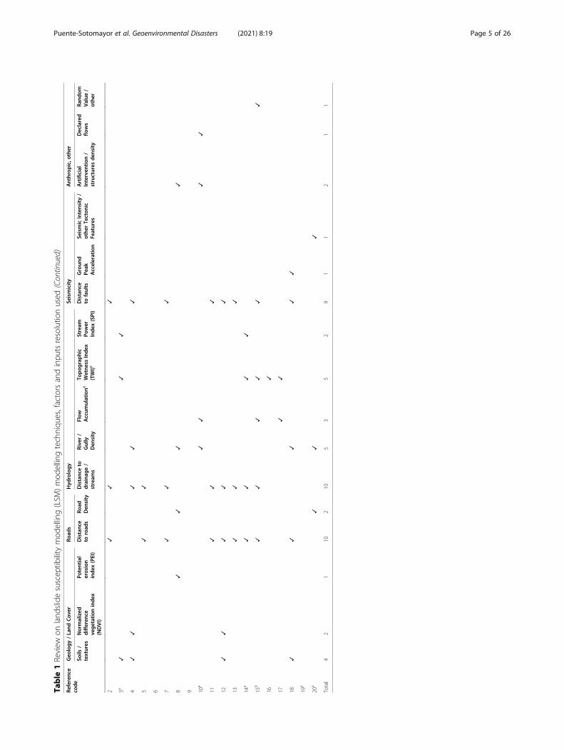
a global review of LSM that the usual determinant fac-tors are slope, geology, and aspect; of these, the first twohave a higher influence on the prediction power ofmodels. They also state that results may vary accordingto methodologies, model validation, landslide types, trig-gering factors, and the researcher background. Otherstudies include precipitation, population density, andland use as significant factors (Hemasinghe et al. 2018;Sepúlveda and Petley 2015).

A brief review on LSMReichenbach et al. (2018) classify landslide susceptibilityassessment into five groups, namely: (i) geomorpho-logical mapping; (ii) analysis of landslide inventories; (iii)heuristic or index-based approaches; (iv) process-basedmethods; and (v) statistical modelling methods. Thepresent work combines the heuristic approach officiallyadopted by the municipality of Quito as a preliminaryinput.

Modelling approaches A number of machine learningmodelling techniques have been developed and ap-plied in diverse locations globally to achieve the finestpossible precision—each time with more sophistica-tion—to provide better inputs into landslide risk re-duction (LRR) policy and planning. Among the mostused LSM techniques during the past two decades aremulti-criteria evaluation (MCE), analytical hierarchicalprocess (AHP), weighted linear combination (WLC),logistic regression (LR), data-driven frequency ratio(FR), random forest (RF), support vector machines(SVM), and artificial neural networks (ANN) (seeTable 1). Most of the applied techniques have beenproven to provide accurate results and differentiatedadvantages, sufficient for LSM practices and, there-fore, LRR zoning policies. For instance, a comparisonbetween LR, SVM, and RF applied to the Sihjhongwatershed, Taiwan, found that RF performed best,whereas LR ran faster (Chang et al. 2019), which canbe useful for large datasets, as in the present work.Regardless of the adopted method, research on LSMfor Andean cities and regions is generally very limitedand only a few application cases have been recentlypublished (Puente-Sotomayor et al. 2021).Modelling for LSM has prompted a discussion on the

impact that different parameters of the process have onthe accuracy of the produced results. In addition to themodelling technique used, these parameters include datapreprocessing, scale or cell/pixel size of input factors,and the type and number of factors used for the model-ling. Table 1 shows a brief comparison of the describedparameters among previous studies.

Relevant LSM parameters Among the most relevantparameters is the preprocessing of data. There are differ-ent techniques to make factors comparable. These in-clude different methods of normalization orstandardization. Terminology varies. This study adoptedthe source assignation of weights in a discrete scale, alsocalled weight-encoding, and data discretization using apercentile scale. Although standardization of weighteddata for landslide susceptibility mapping is still an opendiscussion (Ronchetti et al. 2013), it is considered a validoption whenever intervals between ordinal categories areconsidered equal, regardless of statistical limitationssuch as the limited number of categories and overesti-mation of statistical power (Norman 2010; Pasta 2009;Williams 2019).Regarding the factor parameters for an urban LSM, it

must be noted that only five of the twenty reviewedstudies relate to urban areas. However, even in thesecases, the factors are similar to those applied in theother works, often covering regional scales and rarely in-volving cities, which the current work aims to analyze.Therefore, few previous studies include human/urbanrelated factors, such as the buildings (see factors columnin Table 1), population, and urban road networks, as ap-plied to this work. It is relevant to note that, unless anspecific factor approach or restraints on the availabilityof data are stated, the most considered factors are topog-raphy/digital terrain model (DTM) derivatives (primarilyslope angle, aspect, elevation, and curvature), annualprecipitation, geology (primarily lithology and land use/vegetation coverage), distance to roads, hydrology (pri-marily distance to drainage, density, and topographicwetness index (TWI), which also relates to topography)and distance to faults in the seismicity. Furthermore, be-yond the possibility of including a large number of fac-tors, this does not necessarily mean better performanceof a model and the optimal number of factors in a LSMis still debatable (Catani, Lagomarsino, Segoni, & Tofani2013a).Another discussed parameter in the literature is the

resolution at which the input data is set. Table 1 also in-cludes this parameter for each revised work. Resolutionsvary from 1 to 500m cell sizes. Regardless of the re-straints based on the availability, reliability of data, andthe context itself, some studies have tested the sensitivityof this parameter with diverse approaches and results.For instance, Chang et al. (2019) concluded that the fin-est resolution of topographic data does not necessarilyresult in the best performance of a model. RegardingDTM derivatives, Pawluszek et al. (2018) found in an ex-ample case that the optimal resolution was 30 m, classi-fied by SVM. Another case proved that the 50mresolution contributed best to the performance of an RFtechnique (Catani et al. 2013b). Additional points of


view state that different land-surface factors also havedifferent optimal scales, and that the applied modellingtechnique may also influence this parameterization.Therefore, multiscale approaches are recommended forbetter performance in complex terrain settings (Cataniet al. 2013a Sîrbu et al. 2019). This has also been corrob-orated by Dragićević et al. (2014), who examined thesetypes of complex and multi-scalar contexts from re-gional to municipal and local scales.Once the data is pre-processed and made available for

modelling, one common and simple theoretical modelused is multi-criteria evaluation (MCE), which can becombined with sensitivity analysis, such as in Feizizadehand Blaschke (2014) and Orán Cáceres et al. (2010), andexplained below. A complementary approach to MCE isbinary logistic regression (LOGIT), which is among themost used statistical methods for landslide susceptibilitymapping (Reichenbach et al. 2018). This type of modelhelps to test weighted models, which do not support theassessment of the probability of landslide occurrences(Lombardo and Mai 2018). For this research, a LOGITwas applied, followed by an SA.

Sensitivity analysisA further step in evaluating LOGIT models is to apply anSA (Reichenbach et al. 2018). SA is applied to determinethe contribution of input parameters to the accuracy of themodel prediction appraised in its outputs (Shahri et al.2019; Poelmans and Van Rompaey 2010). The objective ofsensitivity analysis is to help adjust the calibration of thestudied parameters involved in the LSM model to improveits predicting/classification power. Among different meth-odologies, two stand out: the simple, univariate, or “one-at-a-time” (OAT) method, and the stochastic/random-selec-tion method, also called “Monte Carlo”, whose applicationsvary according to the needs of the field of practice (Bouyer2009). Details of both methods are explained in themethods and results sections.

MethodsStudy area and its landslide risk-reduction policybackgroundQuito, the capital of Ecuador, is the most populated oftwo existing metropolitan districts (regions) in the coun-try, with 2,781,641 inhabitants projected for 2020 (INEC2016). The jurisdiction of the Metropolitan District ofQuito (DMQ) covers 4235.2 km2, of which 10% is urbanland with 286,412 housing units (Quito Municipio delDistrito Metropolitano 2015). As one of the Andeanmountain cities, Quito has suffered from multiple nat-ural threats, including landslides, volcano eruptions,floods, and earthquakes. Hence, exposure to risks hasbeen further exacerbated, given the fast populationgrowth and the uncontrolled urbanization process.

Accordingly, Quito has collected geodata relating tolandslide disaster events during the past two decades.This has strengthened the city’s management capacitiesand its approach to preventive policies and actions(Rebotier 2016), in addition to preparedness and re-sponse. Most recently, resiliency has been adopted as anurban policy, to the point of being institutionalized, withthe creation of a Resiliency Department and the designof the city’s resiliency strategy (Quito Alcaldia del Dis-trito Metropolitano 2018; Quito Municipio del DistritoMetropolitano2017).Landslide risk reduction (LRR) policies in Quito have a

history of approximately one decade. They began withlandslide-related land-use zoning as part of the local plan,in 2011 (Puente-Sotomayor et al. 2018). Previously, build-ing regulations included generic risk prevention measures,such as setbacks from ravines, slope borders, and rivers(Concejo del Distrito Metropolitano de Quito 2003). Forlahar-prone areas, a transfer of responsibility from govern-ment to users was used, applying a notarized responsibilityto the owner for building on high-risk areas, prior to cityapproval (Concejo del Distrito Metropolitano de Quito2011). Since 2014, this has no longer been allowed in na-tional laws, which assign criminal liability of the generatedrisks to any official that approves subdivisions or projectsin risk zones (Ecuador Asamblea Nacional 2014).During the past decade, the landslide preventive/re-

ductive approach was materialized by establishing theLRisk zone (ZR) category in the local LUP. Constructionwas strictly banned in ZR areas. This zoning policy intui-tively and imprecisely combined slopes (at the 1:5000scale), soil stability (at the 1:25,000 scale), and field in-spections as the only inputs in 2011. The application ofthis regulation triggered around 40 complaints per yearfrom users, who claimed they were affected socially,through the violation of their housing rights; and, eco-nomically, due to previous investments and rent expec-tations related to the property labeled at-risk. In 2013, areform to this ordinance relaxed the policy by returningto owners the right to build on ZRs, who provided geo-technical studies that justified their projects. This re-vealed limitations of the technical capacity of users andofficials, and the problem with defining “mitigation”,which subsequently evidenced the poor accessibility togeotechnical risk relief for low socio-economic strata. Anew reform in 2015 cancelled the ZR land-use categoryand converted it to an overlay map, which, in practice,did not change the policy (Puente-Sotomayor et al.2018). By 2015, the first landslide susceptibility studieswere produced. The outputs of these studies were ex-pected to improve the ZR policy. However, they havenot yet been articulated with the LUP. These studies’outputs have been labeled as official data and were usedas part of the input data for this research.


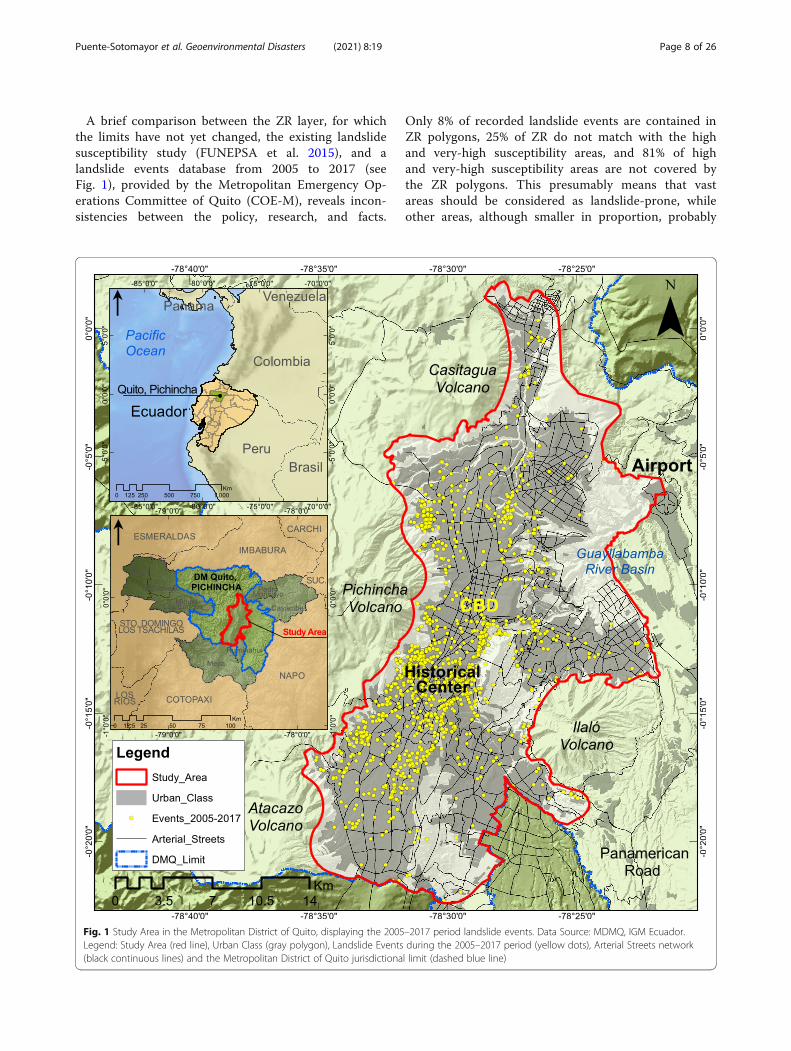
A brief comparison between the ZR layer, for whichthe limits have not yet changed, the existing landslidesusceptibility study (FUNEPSA et al. 2015), and alandslide events database from 2005 to 2017 (seeFig. 1), provided by the Metropolitan Emergency Op-erations Committee of Quito (COE-M), reveals incon-sistencies between the policy, research, and facts.

Only 8% of recorded landslide events are contained inZR polygons, 25% of ZR do not match with the highand very-high susceptibility areas, and 81% of highand very-high susceptibility areas are not covered bythe ZR polygons. This presumably means that vastareas should be considered as landslide-prone, whileother areas, although smaller in proportion, probably

Fig. 1 Study Area in the Metropolitan District of Quito, displaying the 2005–2017 period landslide events. Data Source: MDMQ, IGM Ecuador.Legend: Study Area (red line), Urban Class (gray polygon), Landslide Events during the 2005–2017 period (yellow dots), Arterial Streets network(black continuous lines) and the Metropolitan District of Quito jurisdictional limit (dashed blue line)


do not need a protection policy (Puente-Sotomayoret al. 2018).

Purpose, objectives and scopeThe main purpose of this study was to produce a reliableLandslide Susceptibility Map (LSM) that can supportLRR policies for urban Quito (see study area section).This represents a progress from previous actions regard-ing landslide preventive/reductive zoning in this city. Forthis purpose, specific objectives included the examin-ation of the incidence of urban-related factors in LRisksusceptibility; providing quality inputs for better ZR de-limitation, considering the implications for safety, hous-ing rights, and the economy; and generatingimprovements, further discussion and action in the localLSM processes, by exploring different parameters suchas modelling approaches, scale, data generation, andfactors selection.The practical scope of this study was to derive a land-

slide susceptibility map based on a binary logistic regres-sion model combined with a sensitivity analysis (SA) toprovide optimal calibration options for factor coefficientsused in the model. Developing an evidence-based LSMthat considers SA is an indispensable input for develop-ing an urban policy backed by a socio-political consen-sus (Orán Cáceres et al. 2010). The context ofapplication will be the urban core of the DMQ, includ-ing its surrounding peri-urbanized areas, as describedbelow.This research is built upon data collected during a

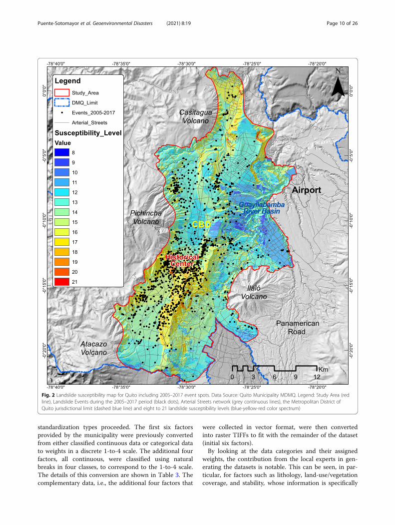
LRisk analysis produced by the municipality in 2015.This study delivered a weighted multi-criteria theoreticalmodel including six factors that were surveyed and proc-essed. These factors are slope, intense precipitations, soilstability after former large landslides, lithology, land use/vegetation coverage, and seismic intensity. Each factorhad partial weights/susceptibilities proposed by local ex-perts in the fields of geotechnics, meteorology, geog-raphy, disaster management, and seismology. The resultsof this model portrayed a landslide susceptibility mapfor Quito and its satellite “conurbated” areas (an ap-proximate total area of 610 km2) using the map algebraGIS tool to sum the partial weights as shown in Fig. 2(FUNEPSA et al. 2015).

Inputs and preprocessingInitially, our study proposed to develop a binary logisticregression model on the basis of six factors identified bythe municipality experts, plus other related to theQuito urban settings, which we aimed to experimentwith. A dataset of landslide events that occurred from2005 to 2017 was therefore collected from the COE-M of Quito. This database includes around 1400events, including rotational and translational

landslides, flows, and topples, all considered generic-ally as landslides (USGS 2004). A minor limitation isthat the dataset suffers from some underreporting,and unbalanced and unstructured elements.From the data of the six initial factors, the first LOGIT

was applied. Then, four additional factors were includedin two steps to test the model. As a first addition, popu-lation, provided by the National Institute of Statisticsand Census (INEC), and floor area, provided by theQuito municipality (MDMQ), were included to con-struct a second LOGIT. Then, road density and buildingfootprint area, also provided by the MDMQ, were addedto run the final LOGIT. All four additional factors werepre-processed and adapted for this research work. As ex-plained in the introduction section, considering theurban context of Quito, where all of the landslide eventswere registered, this research aimed to determine the in-cidence of these factors on the results, whose contentwas more relevant to the urban context, i.e., buildings,streets, and population. Details of all of the ten factorsincluded in this study are provided in Table 2.

ResolutionThe dependent factor, landslide events (binary), and theten independent, explanatory factors were pre-processedin raster files, with a cell size (disaggregation level) of 50m. This was the resolution at which the lithology, landcoverage, seismicity, precipitations, soil stability, andslope were previously provided by the municipality sur-veyors. Complementarily, the additional four “urban”factors were converted from a scale at which the detailof buildings, blocks, and streets was legible (1:1000 ap-proximately), which was logically consistent with the 50m cell size of the other six factors. Therefore, all of thedatasets were standardized to this resolution. In this re-gard, the theoretical background review implied that, al-though scale may determine the modelling performance,performance is also dependent on the context and com-plexity of the process. For this study, although the sec-ondary source input data was pre-processed at a 50 mcell size, an aggregation process through resampling GIStechniques (nearest neighbor mode) were applied to suitthe complete datasets at resolutions of 100, 200, and500 m before the application of the LR modelling foreach resolution. Subsequently, the results provide a ra-tionale to retain the original scale.

StandardizationTo manage a standard scale of factor values before ap-plying the LOGIT, the following process was under-taken. The binary layer of landslide events records oneof two categories for each area unit or cell: true (or one),when one or more landslide events occurred in it; or,false (or zero), when no landslides occurred in it. Two


standardization types proceeded. The first six factorsprovided by the municipality were previously convertedfrom either classified continuous data or categorical datato weights in a discrete 1-to-4 scale. The additional fourfactors, all continuous, were classified using naturalbreaks in four classes, to correspond to the 1-to-4 scale.The details of this conversion are shown in Table 3. Thecomplementary data, i.e., the additional four factors that

were collected in vector format, were then convertedinto raster TIFFs to fit with the remainder of the dataset(initial six factors).By looking at the data categories and their assigned

weights, the contribution from the local experts in gen-erating the datasets is notable. This can be seen, in par-ticular, for factors such as lithology, land-use/vegetationcoverage, and stability, whose information is specifically

Fig. 2 Landslide susceptibility map for Quito including 2005–2017 event spots. Data Source: Quito Municipality MDMQ. Legend: Study Area (redline), Landslide Events during the 2005–2017 period (black dots), Arterial Streets network (grey continuous lines), the Metropolitan District ofQuito jurisdictional limit (dashed blue line) and eight to 21 landslide susceptibility levels (blue-yellow-red color spectrum)


related to the Quito context. Furthermore, It is import-ant to mention that, for the case of the slope factor, theclass “greater than 50°” is weighted as 3 and not 4, asone would suppose. This is due to the fact that most ofthe local geology type, the “cangahua”, found at thisslope range and in most of the study area, is less suscep-tible to landslides than flatter slope ranges and has re-ported much less events, according to the local datamining experts. Regarding the rainfall, the meteorologysurveyors stated that the Quito region is not affected bylong-term persistent rainfall, which triggers landslides inother parts of the world, such as Central America orSoutheast Asia, or in territories affected by El Niño phe-nomena extreme events, which are not regular in termsof time cycles and occur every 25 or 30 years. Instead, inQuito, landslides are more likely triggered by intenseprecipitations, which is why this variable was includedinstead of other climate-related factors, such as annualprecipitation rates. Inclusive, long precipitation was notconsidered in the reviewed scientific articles, as shownin Table 1.A second standardization process for the ten explana-

tory factors was applied and tested. It was based on apercentile discretization. The aim of applying percentilediscretization was to have a finer value than the 1-to-4scale. This also helped to correct a distortion existing inthe provided data, produced by a marginal portion ofoutliers that widened the absolute value range of thedataset, which is an advantage of this discretizationmethod (Grzenda 2020). This distortion occurred

particularly with the data of the floor area and buildingfootprint area. Table 4 shows how the ten factors werediscretized through percentiles. The categorical dataweights were assigned to their corresponding percentileof the 1-to-100 scale, considering in it three equal seg-ments (assuming intervals between weights as equalunits in a discrete scale). For the remaining continuousdata factors, the new values were simply the correspond-ing percentile.

Logistic regressionFollowing the preparation of the data, the LOGIT pro-ceeded. In regard to the sampling method, two sets of el-ements (the binary sample of cells) with equal numberof items were then selected to test the LOGIT. The firstset had cells that registered the occurrence of landslides(an average of 1.29 events per cell), in total, 1139 cellswith a true/one value. The second set had cells that didnot register landslides, i.e., false/zero value. Consideringthe 1139 true values, an equal number of false value cellswere randomly chosen from more than 222,000remaining equivalent value cells in the study area.A generalized linear model regression function in the

programming platform (MATLAB_R2018b) was thenapplied to obtain the values of the coefficients for all tenfactors and the intercept of the function. With thesevalues, the logistic regression (Eq. 1) was applied to ob-tain the landslide susceptibility values for all cells for thestudy area. These values provide the probability of oc-currence of a landslide, varying from 0 (null probability)

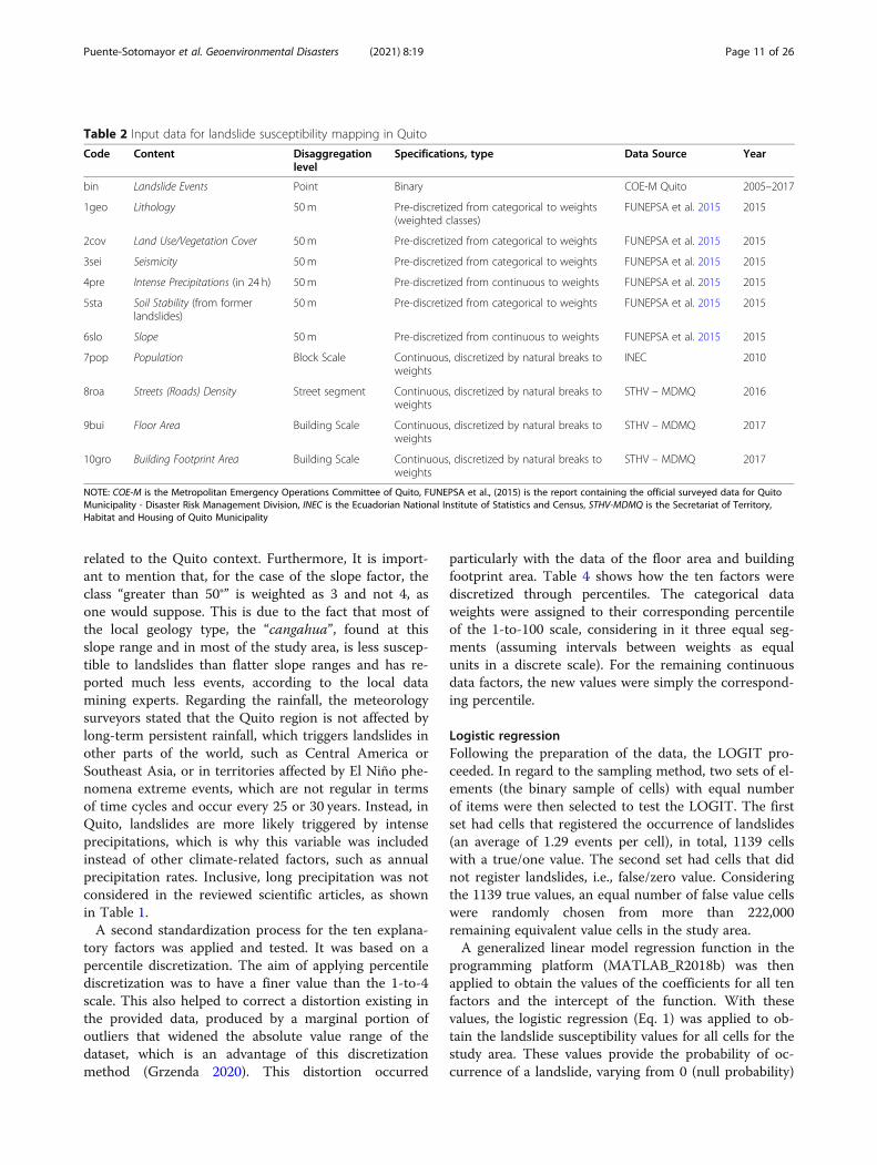
Table 2 Input data for landslide susceptibility mapping in Quito

Code Content Disaggregationlevel

Specifications, type Data Source Year

bin Landslide Events Point Binary COE-M Quito 2005–2017

1geo Lithology 50m Pre-discretized from categorical to weights(weighted classes)

FUNEPSA et al. 2015 2015

2cov Land Use/Vegetation Cover 50m Pre-discretized from categorical to weights FUNEPSA et al. 2015 2015

3sei Seismicity 50m Pre-discretized from categorical to weights FUNEPSA et al. 2015 2015

4pre Intense Precipitations (in 24 h) 50 m Pre-discretized from continuous to weights FUNEPSA et al. 2015 2015

5sta Soil Stability (from formerlandslides)

50 m Pre-discretized from categorical to weights FUNEPSA et al. 2015 2015

6slo Slope 50m Pre-discretized from continuous to weights FUNEPSA et al. 2015 2015

7pop Population Block Scale Continuous, discretized by natural breaks toweights

INEC 2010

8roa Streets (Roads) Density Street segment Continuous, discretized by natural breaks toweights

STHV – MDMQ 2016

9bui Floor Area Building Scale Continuous, discretized by natural breaks toweights

STHV – MDMQ 2017

10gro Building Footprint Area Building Scale Continuous, discretized by natural breaks toweights

STHV – MDMQ 2017

NOTE: COE-M is the Metropolitan Emergency Operations Committee of Quito, FUNEPSA et al., (2015) is the report containing the official surveyed data for QuitoMunicipality - Disaster Risk Management Division, INEC is the Ecuadorian National Institute of Statistics and Census, STHV-MDMQ is the Secretariat of Territory,Habitat and Housing of Quito Municipality


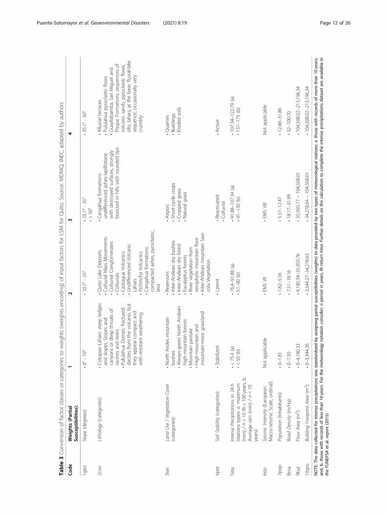
Table

3Con

versionof

factor

classesor

catego

riesto

weigh

ts(weigh

tsen

coding

)of

inpu

tfactorsforLSM

forQuito.Sou

rce:MDMQ,INEC

,adapted

byauthors

Cod

eWeights(Partial

Suscep

tibilities):

12

34

1geo

Slope(deg

rees):

•0°

-10°

•10.1°-25°

•25.1°-35°

•>50°

•35.1°-50°

2cov

Lithology(categ

ories):

•Cotop

axiLahars:steepledg

esandslop

es.Slope

sand

canyon

sor

deep

throatsof

ravine

sandrivers

•Pu

lulahu

aDom

es:fractured

dacitesfro

mthevolcano,bu

tthey

appe

arcompact

and

with

resistantweathering

•Quito

Lake

Dep

osits

•ColluvialMassMovem

ents

•ColluvialCon

glom

erates

•Colluvials

•Casitagu

aVo

lcanics

•Und

ifferen

cedVo

lcanic

Lahars

•PichinchaVo

lcanics

•Cangahu

aform

ations:

compacted

ashe

s,pyroclastic,

lava

•Cangahu

aform

ations:

undifferenced

ashe

s-lapilliston

ewith

destroyedsurfaces,strong

lybisected

inhills

with

roun

dedtip

s

•Alluvialterraces

•Pu

lulahu

apyroclastic

flows

•Guayllabamba,San

Migueland

Pisque

Form

ations:seq

uences

ofvolcanicsand

s,pyroclastic

flows,

silts,lahars;at

thebase:fluvial-lake

sequ

ence,o

ccasionally

very

crum

bly

3sei

Land

Use

/VegetationCo

ver

(categ

ories):

•North

And

esmou

ntain

bushes

•Always-greenNorth

And

ean

high

-mou

ntainforests

•Mou

ntainpasture

•High-mou

ntainand

mou

ntain-moo

rgrassland

•Reservoirs

•Inter-And

eandrybu

shes

•Inter-And

eandryforest

•Eucalyptus

forests

•Rivervege

tatio

nfro

mxeroph

yticmou

ntainfloor

•Inter-And

eanmou

ntainSaxi-

colaVege

tatio

n

•Airp

ort

•Short-cyclecrop

s•Cropp

edgrass

•Naturalgrass

•Quarries

•Bu

ildings

•Erod

edsoils

4pre

SoilStability(categ

ories):

•Stabilized

•Latent

•Reactivated

•Colluvial

•Active

5sta

IntensePrecipitations

in24

h(statio

nstype

s:a.maximum

(mm)/n>10

Rt=100years,b.

Average

rain

(mm)/n<10

years):

•<75.4(a)

•<50

(b)

•76.4–91.88

(a)

•51–90(b)

•91.88–107.34

(a)

•91–130

(b)

•107.34–122.79(a)

•137–175(b)

6slo

Seism

icIntensity

(Europ

ean

Macro-seism

icScale,ordinal):

Not

applicable

•EM

SVII

•EM

SVIII

Not

applicable

7pop

Population(Inhabitants):

•0–1.81

•1.82–5.56

•5.57–12.47

•12.48–31.86

8roa

Road

Density(m

/Ha):

•0–7.50

•7.51–18.16

•18.17–31.99

•32–100.70

9bui

FloorArea

(m2 ):

•0–4,180.33

•4,180.34–35,950.76

•35,950.77–104,508.01

•104,508.02–213,196.34

10gro

BuildingFootprintArea

(m2 ):

•0–3,344.26

•3,344.27–34,278.63

•34,278.64–104,508.01

•104,508.02–213,196.34

NOTE:The

data

collected

forintenseprecipita

tions

was

stan

dardized

byassign

ingpa

rtialsusceptibilitie

s(w

eigh

ts)to

data

prov

ided

bytw

otype

sof

meteo

rologicalstatio

ns:a.tho

sewith

recordsof

morethan

10years;

and,

b.thosewith

recordsof

less

than

10years.Fo

rthemeteo

rology

notatio

nconsider:n

perio

din

years,Rt

return

time.Fu

rthe

rde

tails

onthecalculationto

completetheintenseprecipita

tions

datasetareavailablein

theFU

NEP

SAet

al.rep

ort(201

5)


to 1 (absolute occurrence). These values helped generatethe reference landslide susceptibility map. This processwas first undertaken for the six initial factors; second,with the addition of population and floor area as newfactors; and finally, with the addition of road density andbuilding footprint area. The area under the receiving op-erating characteristic (ROC) curve (AUC) was the per-formance indicator chosen for the LOGIT model,considering it is common in evaluation of the predictionaccuracy of models for natural hazards (Shahri et al.2019; Wang et al. 2020).Equation 1 Logistic regression function for landslide

susceptibility mapping

ls ¼ 11þ e− b0þb1x1þb2x2þ::…þbnxn:ð Þ

where:ls = landslide susceptibility: the probability of occur-

rence of a landslide (between 0 and 1)e = the mathematical constant e (2.71828)b0 = the intercept of the logistic functionbn = the coefficient of factor xnxn = the factor number n

Sensitivity Analysis – univariate methodAfter the generation of a referential susceptibility mapand the validation of the LOGIT model that generated itusing the AUC/ROC value, SA was performed to testthe sensitivity of the model outputs to changes in one,many, or all selected parameters. For this research, theselected referential metric was the AUC value as theoutput for all of the generated simulations, as applied toSA by Poelmans and Van Rompaey (2010). Sensitivityanalyses were performed using two methods.The first was the simple, univariate, or OAT method,

which is simple to apply and assess. It consisted in chan-ging one “free” parameter of the model at a time to gen-erate variations of the model, within a defined range andwith a defined interval for the changes. In this case,while one factor changes its coefficient, the others re-main unaffected (fixed parameters) and remain as the

references. For the model used in this research, the pa-rameters changed were each of the ten coefficients gen-erated by the LOGIT model. A set of multipliers rangingfrom 0.1 to 20 with an interval of 0.1 modified each ofthe coefficients of the ten factors, one at a time, to gen-erate a total of 2000 susceptibility maps, from whichAUC values (outputs) were generated and plotted. TheAUC values higher than the reference AUC value (thefirst generated) indicates that their correspondingmodels are better calibrated than the reference. This wasreproduced for the weights-encoded and the percentile-discretized models.

Kolmogorov–Smirnov test for sensitivityA two-sample Kolmogorov–Smirnov (K-S) test was ap-plied to the univariate test results for both weights andpercentile-based discretization methods as another meansto determine the sensitivity of the factors. As a metric, theD-statistic (also called the KS-statistic) values are pro-vided, indicating the D-critical value, as calculated usingEq. 2. These provide a more insightful picture than the p-values of the same test, which considered an alpha valueof 0.05 and were also calculated. The K-S tests were tabu-lated using the empirical distribution functions of twosamples—ones and zeros—from each resulting map de-rived from the changes of the simple/univariate method,i.e., the distribution of the cell values corresponding toevent occurrence cells (1139 observations/elements) com-pared to a distribution of a randomly selected similarnumber of non-occurrence cells. This test was appliedonly to the results of the simple sensitivity analysis due tolimitations in computer processing capacities and simpli-city of visualization in charts, which provided for bettercommunication of results.Equation 2 Calculation of the D-critical value for a

two-sample K-S test

Dα ¼ c αð Þffiffiffiffiffiffiffiffiffiffiffiffiffiffiffi

n1 þ n2n1n2

r

where:

Table 4 Conversion table of categorical data from weights encoding to percentile discretization, and continuous data to percentiles

Categorical Data Factors: • Lithology• Land Use/Vegetation Coverage• Seismic intensities• Intense Precipitations• Soil Stability after former landslide events

Weights (Partial Susceptibilities) a: 1 2 3 4

Percentile Values: 1 33 67 100

Continuous Data Factors: • Slope• Population• Road Density• Floor Area• Building Footprint Area

Weights (Partial Susceptibilities) b: 1 2 3 4

Percentile Values: Corresponding percentile (from 1to 100)

aAssigned according to FUNEPSA et al. (2015)bClassified by natural breaks, except for slope, classified according to FUNEPSA et al. (2015)


Dα = D-critical value of the K-S test at an alpha valueαα = Alpha value determined for the K-S test (0.05 for

this case)c(α) = constant based on α (1.36 for this case)n1 = first sample size (1139 for this case)n2 = second sample size (1139 for this case)

Sensitivity Analysis—Monte Carlo methodA second method to test the sensitivity based on factorsused random variations for all of the factors, from oneto all at a time, also within a defined range and with adefined interval. This is also called the Monte Carlo orstochastic method. For this research, multipliers of oneor more coefficients at a time ranged from 0.1 to 5 withan interval of 0.1. The number of simulations for thisrandom selection of possibilities was set to 8000, whichmay vary in replications of this study, according to thecomputer’s processing capacities. Once again, AUCvalues (outputs) were generated and those higher thanthe reference AUC value indicated that their corre-sponding models with their modified coefficients’ valueshad a better performance calibration than the referenceitself (Bouyer 2009). To better illustrate this, a table ofrandom simulation calibrations is provided in the re-sults, plus a chart showing the two best predictorfactors.

Methodology summary and software usedTo summarize, Table 5 shows all of the methodologyand specific tools applied for this research.Regarding the software packages used to process data

for this research work, GIS software (ArcMap 10.3) wasapplied to produce all maps using the integration, trans-formation, and geoprocessing tools, and conversion ofshapefiles into raster TIFF files to make them suitablefor calculation for the LOGIT model and the SA. A pro-gramming platform for matrix analysis (MATLAB_R2018b) was used for the SA, for which, particularly the

generalized linear model regression, (glmfit function)and the AUC value computation (perfcurve function),were applied. For the two-sample K-S test, the functionused was kstest2. The subsequent outputs were TIFFfiles for mapping and CSV datasets to produce graphsand charts in a spreadsheet package (Microsoft Excel)and a presentation/illustration package (Micro-soft PowerPoint). Tables were adjusted to a word pro-cessing package (Microsoft Word) format. The inputTIFF files and the programming platform (MATLAB_R2018b) code are provided as Supplementary Materialto this research work

ResultsLOGIT results by adding urban factors and astandardization variantThe first results portray the changes regarding theaddition of factors, departing from the six-factor initialLOGIT model, which corresponds to the map shown inFig. 2, which delivered weight scores from eight (lowestlandslide susceptibility) to 21 (highest landslide suscepti-bility). This considered six factors: lithology, land use/vegetation coverage, seismic intensities, intense precipita-tions, soil stability after large events, and slope. Subse-quently, the LOGIT was tested with eight factors andfinally with 10 factors. The eight-factor model includedtwo more factors: population and floor area, whileretaining the weights encoding (continuous factors clas-sified by natural breaks). The 10-factor model includedtwo more factors: road density and building footprintarea, also weights-encoded. As new factors were added,the coefficients with the highest values changed theirrelative descending order (from highest to lowest value).For the 10-factor model, a variation by percentile-discretization of factor values was applied, which deliv-ered a fourth set of results. The four models’ results, in-cluding their corresponding AUC value, can be seen inTable 6. The initial multi-criteria evaluation (MCE) offi-cial map and the 6, 8, and 10-factor reference maps

Table 5 Methodology summary and applied tools

6-Factor Model 8-Factor Model 10-Factor Model

Weights-encoding Weights-encoding Weights-encoding Percentile-discretization

LOGIT with referential landslide susceptibilitymap and AUC value

✓ ✓ ✓ ✓

Resolution tests of 50, 100, 200 and 500mcell size, through LOGIT and AUC value

✓

Sensitivity Analysis – Univariate method,variations plot and AUC values higherthan reference

✓ ✓

K-S test ✓ ✓

Sensitivity Analysis – Monte Carlo Method,visualization of 2 best predictors and AUCvalues higher than reference

✓ ✓


(weights and percentile standardizations), can be seen inFig. 3. The last two maps (d and e) in this figure wereused for SA.

Results based on resolution inputsA previous approach in addition to testing SA based onfactors, was to consider the impact of the variation in theinput data cell size on the final result, using the AUCvalue as a metric of validation. To test this sensitivity, theminimum resolution (50m) provided by the sources as in-put data was resampled to 100, 200, and 500m. The se-lected standardization method for this test was theweighed-encoding approach because it performed with ahigher AUC value than the percentile-discretized model(see Table 6). To illustrate changes based on resolution in-puts, Table 7 shows the descriptive statistics of AUCvalues after simulating 100 LSM units for each of the citedcell sizes. It can be noted that the highest average AUCvalue corresponds to the 500m cell case. Nonetheless, themodel corresponding to this cell size is the least stable, asindicated by its standard deviation and range, which arehigher than the cases of the other cell sizes. In contrast,the original 50m cell size provided more stable behaviorwhile maintaining a reasonable and reliable AUC value be-fore testing other parameters for SA.

Univariate SA resultsWith the ten-factor model, executed by bothstandardization methods (weights and percentiles), an SAbased on factors was performed. For the weights-encodingmethod, the univariate SA produced susceptibility maps

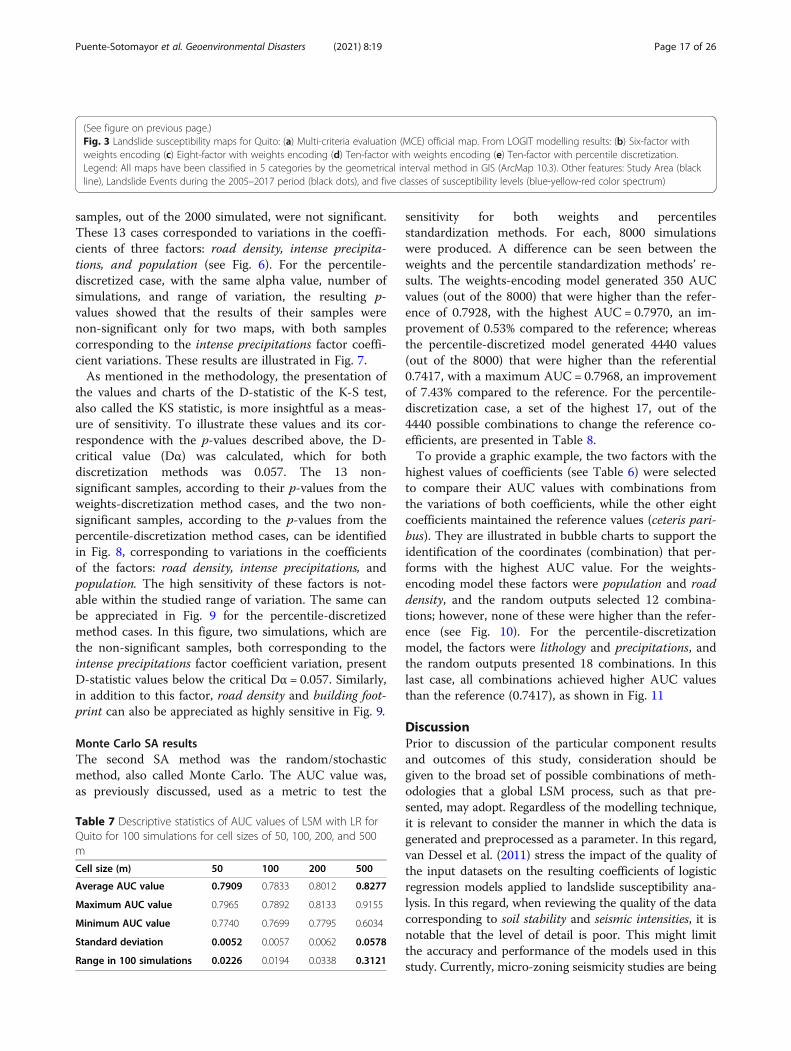
whose AUC values (the metric of the sensitivity) were plot-ted, as seen in Fig. 4. From this analysis, and from the rangeand interval set to produce the coefficient variations, therewere 241 AUC values higher than the reference AUC value(0.7928) out of 2000 simulations. When observing thischart, the AUC improvement is slightly higher than the ref-erence. From the 2000 simulations, the highest AUC valuewas 0.7943, which is almost 0.2% higher than the reference.The coefficients that had the strongest impacts on the re-sults, when the variations were applied, belong to the popu-lation, slope, and road density factors.The same test was applied to the percentile-discretized

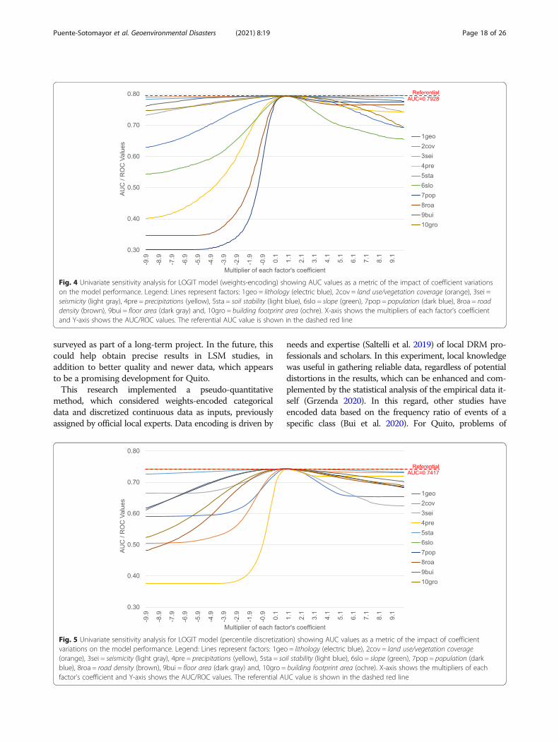
case. The results delivered 34 AUC values higher than thereference AUC value (0.7417) out of 2000 programmedsimulations. The maximum improvement reached anAUC value of 0.7419 with a marginal improvement of0.03%. The plotting of all AUC values derived from thisunivariate method variations’ susceptibility maps/datasetscan be seen in Fig. 5. Precipitations, land-use cover, androad density stand out as the most sensitive factors withinthe defined range of variations. It must be noted that roaddensity is among the most sensitive factors for bothstandardization methods, although it is not the mostsensitive in either of them.

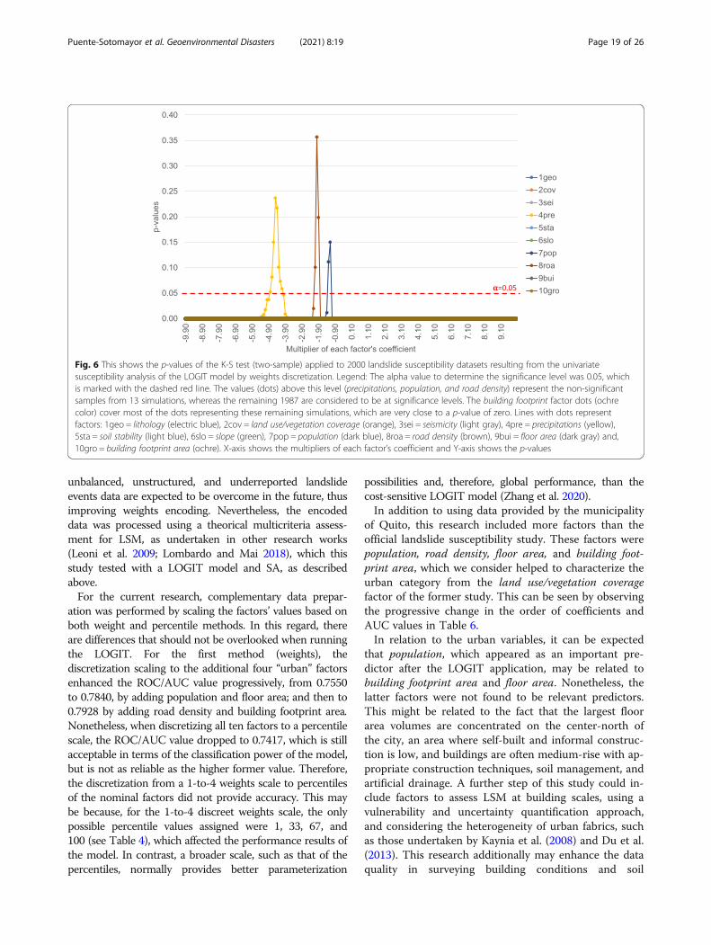
K-S test resultsAs an alternative means to measure sensitivity, the K-Stest was applied to the same simulations undertaken forthe univariate SA, including range and interval varia-tions. Regarding the K-S test applied to the weights-encoding method, the p-value (at an alpha value of 0.05)showed that 13 resulting landslide susceptibility map

Table 6 Output values from LOGIT modelling for landslide susceptibility in Quito

Code Factor 6-Factor Model 8-Factor Model 10-Factor Model

Weights encoding Weights encoding Weights encoding Percentile discretization

Coefficient(β value)

DescendingOrder


DescendingOrder


DescendingOrder


DescendingOrder

0int Intercept −0.5281 −10.7830 −4.1375 −2.4317

1geo Lithology 0.3756 3 0.2550 5 0.1905 5 0.0160 2

2cov Land use/vegetation coverage 0.8483 1 0.4250 4 0.0125 7 0.0122 3

3sei Seismic Intensity −0.1628 6 −0.0910 7 −0.2004 9 −0.0110 10

4pre Intense Precipitations 0.6528 2 0.4500 2 0.3943 3 0.0238 1

5sta Stability after large events 0.0247 5 0.1160 6 −0.1526 8 0.0047 5

6slo Slope 0.3756 4 0.4450 3 0.3896 4 −0.00045 7

7pop Population – – 0.6840 1 0.5348 2 0.0034 6

8roa Road Density – – – – 0.6101 1 0.0052 4

9bui Floor Area – – −0.1280 8 0.0566 6 −0.0040 9

10gro Building Footprint Area – – – – −0.2364 10 −0.0038 8

AUC value 0.755 0.784 0.7928 0.7417

NOTE: Descending Order columns refer to the relative order position that explanatory factor coefficients have among their group in the model by sorting themfrom the highest to the lowest value


Fig. 3 (See legend on next page.)


samples, out of the 2000 simulated, were not significant.These 13 cases corresponded to variations in the coeffi-cients of three factors: road density, intense precipita-tions, and population (see Fig. 6). For the percentile-discretized case, with the same alpha value, number ofsimulations, and range of variation, the resulting p-values showed that the results of their samples werenon-significant only for two maps, with both samplescorresponding to the intense precipitations factor coeffi-cient variations. These results are illustrated in Fig. 7.As mentioned in the methodology, the presentation of

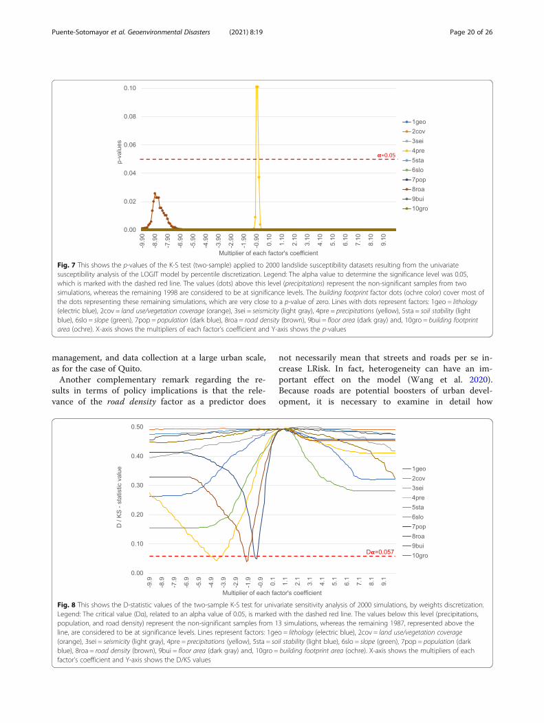
the values and charts of the D-statistic of the K-S test,also called the KS statistic, is more insightful as a meas-ure of sensitivity. To illustrate these values and its cor-respondence with the p-values described above, the D-critical value (Dα) was calculated, which for bothdiscretization methods was 0.057. The 13 non-significant samples, according to their p-values from theweights-discretization method cases, and the two non-significant samples, according to the p-values from thepercentile-discretization method cases, can be identifiedin Fig. 8, corresponding to variations in the coefficientsof the factors: road density, intense precipitations, andpopulation. The high sensitivity of these factors is not-able within the studied range of variation. The same canbe appreciated in Fig. 9 for the percentile-discretizedmethod cases. In this figure, two simulations, which arethe non-significant samples, both corresponding to theintense precipitations factor coefficient variation, presentD-statistic values below the critical Dα = 0.057. Similarly,in addition to this factor, road density and building foot-print can also be appreciated as highly sensitive in Fig. 9.

Monte Carlo SA resultsThe second SA method was the random/stochasticmethod, also called Monte Carlo. The AUC value was,as previously discussed, used as a metric to test the

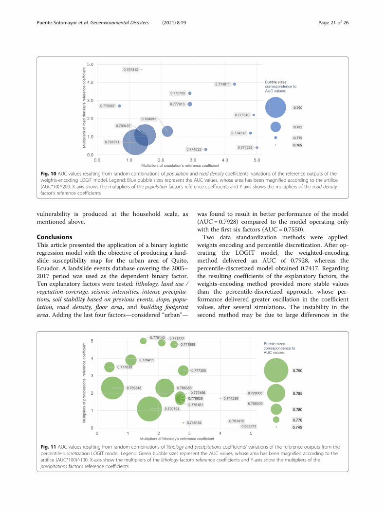
sensitivity for both weights and percentilesstandardization methods. For each, 8000 simulationswere produced. A difference can be seen between theweights and the percentile standardization methods’ re-sults. The weights-encoding model generated 350 AUCvalues (out of the 8000) that were higher than the refer-ence of 0.7928, with the highest AUC = 0.7970, an im-provement of 0.53% compared to the reference; whereasthe percentile-discretized model generated 4440 values(out of the 8000) that were higher than the referential0.7417, with a maximum AUC = 0.7968, an improvementof 7.43% compared to the reference. For the percentile-discretization case, a set of the highest 17, out of the4440 possible combinations to change the reference co-efficients, are presented in Table 8.To provide a graphic example, the two factors with the

highest values of coefficients (see Table 6) were selectedto compare their AUC values with combinations fromthe variations of both coefficients, while the other eightcoefficients maintained the reference values (ceteris pari-bus). They are illustrated in bubble charts to support theidentification of the coordinates (combination) that per-forms with the highest AUC value. For the weights-encoding model these factors were population and roaddensity, and the random outputs selected 12 combina-tions; however, none of these were higher than the refer-ence (see Fig. 10). For the percentile-discretizationmodel, the factors were lithology and precipitations, andthe random outputs presented 18 combinations. In thislast case, all combinations achieved higher AUC valuesthan the reference (0.7417), as shown in Fig. 11

DiscussionPrior to discussion of the particular component resultsand outcomes of this study, consideration should begiven to the broad set of possible combinations of meth-odologies that a global LSM process, such as that pre-sented, may adopt. Regardless of the modelling technique,it is relevant to consider the manner in which the data isgenerated and preprocessed as a parameter. In this regard,van Dessel et al. (2011) stress the impact of the quality ofthe input datasets on the resulting coefficients of logisticregression models applied to landslide susceptibility ana-lysis. In this regard, when reviewing the quality of the datacorresponding to soil stability and seismic intensities, it isnotable that the level of detail is poor. This might limitthe accuracy and performance of the models used in thisstudy. Currently, micro-zoning seismicity studies are being

(See figure on previous page.)Fig. 3 Landslide susceptibility maps for Quito: (a) Multi-criteria evaluation (MCE) official map. From LOGIT modelling results: (b) Six-factor withweights encoding (c) Eight-factor with weights encoding (d) Ten-factor with weights encoding (e) Ten-factor with percentile discretization.Legend: All maps have been classified in 5 categories by the geometrical interval method in GIS (ArcMap 10.3). Other features: Study Area (blackline), Landslide Events during the 2005–2017 period (black dots), and five classes of susceptibility levels (blue-yellow-red color spectrum)

Table 7 Descriptive statistics of AUC values of LSM with LR forQuito for 100 simulations for cell sizes of 50, 100, 200, and 500m

Cell size (m) 50 100 200 500

Average AUC value 0.7909 0.7833 0.8012 0.8277

Maximum AUC value 0.7965 0.7892 0.8133 0.9155

Minimum AUC value 0.7740 0.7699 0.7795 0.6034

Standard deviation 0.0052 0.0057 0.0062 0.0578

Range in 100 simulations 0.0226 0.0194 0.0338 0.3121


surveyed as part of a long-term project. In the future, thiscould help obtain precise results in LSM studies, inaddition to better quality and newer data, which appearsto be a promising development for Quito.This research implemented a pseudo-quantitative

method, which considered weights-encoded categoricaldata and discretized continuous data as inputs, previouslyassigned by official local experts. Data encoding is driven by

needs and expertise (Saltelli et al. 2019) of local DRM pro-fessionals and scholars. In this experiment, local knowledgewas useful in gathering reliable data, regardless of potentialdistortions in the results, which can be enhanced and com-plemented by the statistical analysis of the empirical data it-self (Grzenda 2020). In this regard, other studies haveencoded data based on the frequency ratio of events of aspecific class (Bui et al. 2020). For Quito, problems of

Fig. 4 Univariate sensitivity analysis for LOGIT model (weights-encoding) showing AUC values as a metric of the impact of coefficient variationson the model performance. Legend: Lines represent factors: 1geo = lithology (electric blue), 2cov = land use/vegetation coverage (orange), 3sei =seismicity (light gray), 4pre = precipitations (yellow), 5sta = soil stability (light blue), 6slo = slope (green), 7pop = population (dark blue), 8roa = roaddensity (brown), 9bui = floor area (dark gray) and, 10gro = building footprint area (ochre). X-axis shows the multipliers of each factor’s coefficientand Y-axis shows the AUC/ROC values. The referential AUC value is shown in the dashed red line

Fig. 5 Univariate sensitivity analysis for LOGIT model (percentile discretization) showing AUC values as a metric of the impact of coefficientvariations on the model performance. Legend: Lines represent factors: 1geo = lithology (electric blue), 2cov = land use/vegetation coverage(orange), 3sei = seismicity (light gray), 4pre = precipitations (yellow), 5sta = soil stability (light blue), 6slo = slope (green), 7pop = population (darkblue), 8roa = road density (brown), 9bui = floor area (dark gray) and, 10gro = building footprint area (ochre). X-axis shows the multipliers of eachfactor’s coefficient and Y-axis shows the AUC/ROC values. The referential AUC value is shown in the dashed red line


unbalanced, unstructured, and underreported landslideevents data are expected to be overcome in the future, thusimproving weights encoding. Nevertheless, the encodeddata was processed using a theorical multicriteria assess-ment for LSM, as undertaken in other research works(Leoni et al. 2009; Lombardo and Mai 2018), which thisstudy tested with a LOGIT model and SA, as describedabove.For the current research, complementary data prepar-

ation was performed by scaling the factors’ values based onboth weight and percentile methods. In this regard, thereare differences that should not be overlooked when runningthe LOGIT. For the first method (weights), thediscretization scaling to the additional four “urban” factorsenhanced the ROC/AUC value progressively, from 0.7550to 0.7840, by adding population and floor area; and then to0.7928 by adding road density and building footprint area.Nonetheless, when discretizing all ten factors to a percentilescale, the ROC/AUC value dropped to 0.7417, which is stillacceptable in terms of the classification power of the model,but is not as reliable as the higher former value. Therefore,the discretization from a 1-to-4 weights scale to percentilesof the nominal factors did not provide accuracy. This maybe because, for the 1-to-4 discreet weights scale, the onlypossible percentile values assigned were 1, 33, 67, and100 (see Table 4), which affected the performance results ofthe model. In contrast, a broader scale, such as that of thepercentiles, normally provides better parameterization

possibilities and, therefore, global performance, than thecost-sensitive LOGIT model (Zhang et al. 2020).In addition to using data provided by the municipality

of Quito, this research included more factors than theofficial landslide susceptibility study. These factors werepopulation, road density, floor area, and building foot-print area, which we consider helped to characterize theurban category from the land use/vegetation coveragefactor of the former study. This can be seen by observingthe progressive change in the order of coefficients andAUC values in Table 6.In relation to the urban variables, it can be expected

that population, which appeared as an important pre-dictor after the LOGIT application, may be related tobuilding footprint area and floor area. Nonetheless, thelatter factors were not found to be relevant predictors.This might be related to the fact that the largest floorarea volumes are concentrated on the center-north ofthe city, an area where self-built and informal construc-tion is low, and buildings are often medium-rise with ap-propriate construction techniques, soil management, andartificial drainage. A further step of this study could in-clude factors to assess LSM at building scales, using avulnerability and uncertainty quantification approach,and considering the heterogeneity of urban fabrics, suchas those undertaken by Kaynia et al. (2008) and Du et al.(2013). This research additionally may enhance the dataquality in surveying building conditions and soil

Fig. 6 This shows the p-values of the K-S test (two-sample) applied to 2000 landslide susceptibility datasets resulting from the univariatesusceptibility analysis of the LOGIT model by weights discretization. Legend: The alpha value to determine the significance level was 0.05, whichis marked with the dashed red line. The values (dots) above this level (precipitations, population, and road density) represent the non-significantsamples from 13 simulations, whereas the remaining 1987 are considered to be at significance levels. The building footprint factor dots (ochrecolor) cover most of the dots representing these remaining simulations, which are very close to a p-value of zero. Lines with dots representfactors: 1geo = lithology (electric blue), 2cov = land use/vegetation coverage (orange), 3sei = seismicity (light gray), 4pre = precipitations (yellow),5sta = soil stability (light blue), 6slo = slope (green), 7pop = population (dark blue), 8roa = road density (brown), 9bui = floor area (dark gray) and,10gro = building footprint area (ochre). X-axis shows the multipliers of each factor’s coefficient and Y-axis shows the p-values


management, and data collection at a large urban scale,as for the case of Quito.Another complementary remark regarding the re-

sults in terms of policy implications is that the rele-vance of the road density factor as a predictor does

not necessarily mean that streets and roads per se in-crease LRisk. In fact, heterogeneity can have an im-portant effect on the model (Wang et al. 2020).Because roads are potential boosters of urban devel-opment, it is necessary to examine in detail how

Fig. 7 This shows the p-values of the K-S test (two-sample) applied to 2000 landslide susceptibility datasets resulting from the univariatesusceptibility analysis of the LOGIT model by percentile discretization. Legend: The alpha value to determine the significance level was 0.05,which is marked with the dashed red line. The values (dots) above this level (precipitations) represent the non-significant samples from twosimulations, whereas the remaining 1998 are considered to be at significance levels. The building footprint factor dots (ochre color) cover most ofthe dots representing these remaining simulations, which are very close to a p-value of zero. Lines with dots represent factors: 1geo = lithology(electric blue), 2cov = land use/vegetation coverage (orange), 3sei = seismicity (light gray), 4pre = precipitations (yellow), 5sta = soil stability (lightblue), 6slo = slope (green), 7pop = population (dark blue), 8roa = road density (brown), 9bui = floor area (dark gray) and, 10gro = building footprintarea (ochre). X-axis shows the multipliers of each factor’s coefficient and Y-axis shows the p-values

Fig. 8 This shows the D-statistic values of the two-sample K-S test for univariate sensitivity analysis of 2000 simulations, by weights discretization.Legend: The critical value (Dα), related to an alpha value of 0.05, is marked with the dashed red line. The values below this level (precipitations,population, and road density) represent the non-significant samples from 13 simulations, whereas the remaining 1987, represented above theline, are considered to be at significance levels. Lines represent factors: 1geo = lithology (electric blue), 2cov = land use/vegetation coverage(orange), 3sei = seismicity (light gray), 4pre = precipitations (yellow), 5sta = soil stability (light blue), 6slo = slope (green), 7pop = population (darkblue), 8roa = road density (brown), 9bui = floor area (dark gray) and, 10gro = building footprint area (ochre). X-axis shows the multipliers of eachfactor’s coefficient and Y-axis shows the D/KS values


vulnerability is produced at the household scale, asmentioned above.

ConclusionsThis article presented the application of a binary logisticregression model with the objective of producing a land-slide susceptibility map for the urban area of Quito,Ecuador. A landslide events database covering the 2005–2017 period was used as the dependent binary factor.Ten explanatory factors were tested: lithology, land use /vegetation coverage, seismic intensities, intense precipita-tions, soil stability based on previous events, slope, popu-lation, road density, floor area, and building footprintarea. Adding the last four factors—considered “urban”—

was found to result in better performance of the model(AUC = 0.7928) compared to the model operating onlywith the first six factors (AUC = 0.7550).Two data standardization methods were applied:

weights encoding and percentile discretization. After op-erating the LOGIT model, the weighted-encodingmethod delivered an AUC of 0.7928, whereas thepercentile-discretized model obtained 0.7417. Regardingthe resulting coefficients of the explanatory factors, theweights-encoding method provided more stable valuesthan the percentile-discretized approach, whose per-formance delivered greater oscillation in the coefficientvalues, after several simulations. The instability in thesecond method may be due to large differences in the

Fig. 10 AUC values resulting from random combinations of population and road density coefficients' variations of the reference outputs of theweights-encoding LOGIT model. Legend: Blue bubble sizes represent the AUC values, whose area has been magnified according to the artifice(AUC*10)^200. X-axis shows the multipliers of the population factor’s reference coefficients and Y-axis shows the multipliers of the road densityfactor’s reference coefficients

Fig. 11 AUC values resulting from random combinations of lithology and precipitations coefficients' variations of the reference outputs from thepercentile-discretization LOGIT model. Legend: Green bubble sizes represent the AUC values, whose area has been magnified according to theartifice (AUC*100)^100. X-axis show the multipliers of the lithology factor’s reference coefficients and Y-axis show the multipliers of theprecipitations factor’s reference coefficients


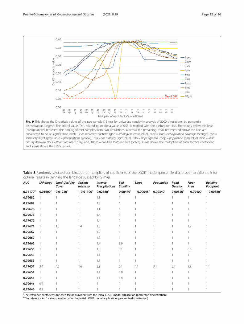
Fig. 9 This shows the D-statistic values of the two-sample K-S test for univariate sensitivity analysis of 2000 simulations, by percentilediscretization. Legend: The critical value (Dα), related to an alpha value of 0.05, is marked with the dashed red line. The values below this level(precipitations) represent the non-significant samples from two simulations, whereas the remaining 1998, represented above the line, areconsidered to be at significance levels. Lines represent factors: 1geo = lithology (electric blue), 2cov = land use/vegetation coverage (orange), 3sei =seismicity (light gray), 4pre = precipitations (yellow), 5sta = soil stability (light blue), 6slo = slope (green), 7pop = population (dark blue), 8roa = roaddensity (brown), 9bui = floor area (dark gray) and, 10gro = building footprint area (ochre). X-axis shows the multipliers of each factor’s coefficientand Y-axis shows the D/KS values

Table 8 Randomly selected combination of multipliers of coefficients of the LOGIT model (percentile-discretized) to calibrate it foroptimal results in defining the landslide susceptibility map

AUC Lithology Land Use/VegCover

SeismicIntensity

IntensePrecipitations

SoilStability

Slope Population RoadDensity

FloorArea

BuildingFootprint

0.74170b 0.01600a 0.01220a − 0.01100a 0.02380a 0.00470a − 0.00045a 0.00340a 0.00520a − 0.00400a − 0.00380a

0.79682 1 1 1 1.3 1 1 1 1 1 1

0.79682 1 1 1 1.3 1 1 1 1 1 1

0.79676 1 1 1 1.4 1 1 1 1 1 1

0.79676 1 1 1 1.4 1 1 1 1 1 1

0.79676 1 1 1 1.4 1 1 1 1 1 1

0.79671 1 1.5 1.4 1.3 1 1 1 1 1.9 1

0.79667 1 1 1 1.2 1 1 1 1 1 1

0.79667 1 1 1 1.2 1 1 1 1 1 1

0.79662 1 1 1 1.4 3.9 1 1 1 1 1

0.79655 1 1 1 1.5 3.1 1 1 1 0.3 1

0.79653 1 1 1 1.1 1 1 1 1 1 1

0.79653 1 1 1 1.1 1 1 1 1 1 1

0.79651 3.4 4.2 1.6 3.9 0.1 4.1 3.1 3.7 2.9 1.1

0.79651 1 1 1 1.1 1.8 1 1 1 1 1

0.79651 1 1 1 1.1 1.8 1 1 1 1 1

0.79646 0.9 1 1 1 1 1 1 1 1 1

0.79646 0.9 1 1 1 1 1 1 1 1 1aThe reference coefficients for each factor provided from the initial LOGIT model application (percentile-discretization)bThe reference AUC values provided after the initial LOGIT model application (percentile-discretization)


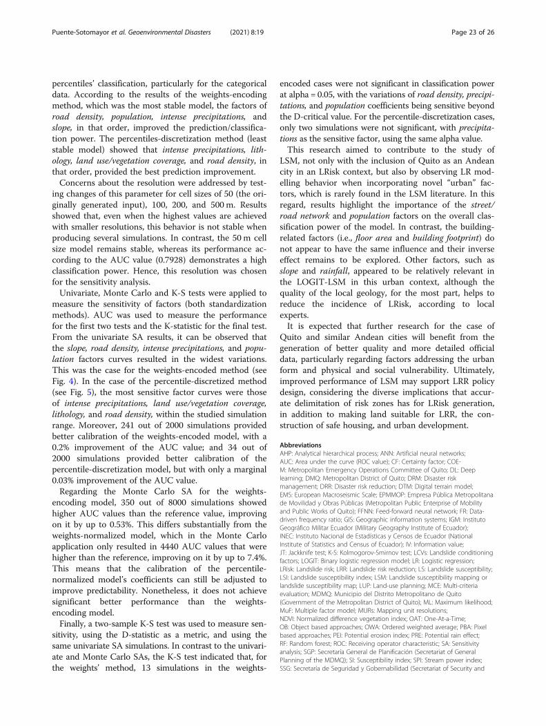
percentiles’ classification, particularly for the categoricaldata. According to the results of the weights-encodingmethod, which was the most stable model, the factors ofroad density, population, intense precipitations, andslope, in that order, improved the prediction/classifica-tion power. The percentiles-discretization method (leaststable model) showed that intense precipitations, lith-ology, land use/vegetation coverage, and road density, inthat order, provided the best prediction improvement.Concerns about the resolution were addressed by test-

ing changes of this parameter for cell sizes of 50 (the ori-ginally generated input), 100, 200, and 500 m. Resultsshowed that, even when the highest values are achievedwith smaller resolutions, this behavior is not stable whenproducing several simulations. In contrast, the 50 m cellsize model remains stable, whereas its performance ac-cording to the AUC value (0.7928) demonstrates a highclassification power. Hence, this resolution was chosenfor the sensitivity analysis.Univariate, Monte Carlo and K-S tests were applied to

measure the sensitivity of factors (both standardizationmethods). AUC was used to measure the performancefor the first two tests and the K-statistic for the final test.From the univariate SA results, it can be observed thatthe slope, road density, intense precipitations, and popu-lation factors curves resulted in the widest variations.This was the case for the weights-encoded method (seeFig. 4). In the case of the percentile-discretized method(see Fig. 5), the most sensitive factor curves were thoseof intense precipitations, land use/vegetation coverage,lithology, and road density, within the studied simulationrange. Moreover, 241 out of 2000 simulations providedbetter calibration of the weights-encoded model, with a0.2% improvement of the AUC value; and 34 out of2000 simulations provided better calibration of thepercentile-discretization model, but with only a marginal0.03% improvement of the AUC value.Regarding the Monte Carlo SA for the weights-

encoding model, 350 out of 8000 simulations showedhigher AUC values than the reference value, improvingon it by up to 0.53%. This differs substantially from theweights-normalized model, which in the Monte Carloapplication only resulted in 4440 AUC values that werehigher than the reference, improving on it by up to 7.4%.This means that the calibration of the percentile-normalized model’s coefficients can still be adjusted toimprove predictability. Nonetheless, it does not achievesignificant better performance than the weights-encoding model.Finally, a two-sample K-S test was used to measure sen-

sitivity, using the D-statistic as a metric, and using thesame univariate SA simulations. In contrast to the univari-ate and Monte Carlo SAs, the K-S test indicated that, forthe weights’ method, 13 simulations in the weights-

encoded cases were not significant in classification powerat alpha = 0.05, with the variations of road density, precipi-tations, and population coefficients being sensitive beyondthe D-critical value. For the percentile-discretization cases,only two simulations were not significant, with precipita-tions as the sensitive factor, using the same alpha value.This research aimed to contribute to the study of

LSM, not only with the inclusion of Quito as an Andeancity in an LRisk context, but also by observing LR mod-elling behavior when incorporating novel “urban” fac-tors, which is rarely found in the LSM literature. In thisregard, results highlight the importance of the street/road network and population factors on the overall clas-sification power of the model. In contrast, the building-related factors (i.e., floor area and building footprint) donot appear to have the same influence and their inverseeffect remains to be explored. Other factors, such asslope and rainfall, appeared to be relatively relevant inthe LOGIT-LSM in this urban context, although thequality of the local geology, for the most part, helps toreduce the incidence of LRisk, according to localexperts.It is expected that further research for the case of

Quito and similar Andean cities will benefit from thegeneration of better quality and more detailed officialdata, particularly regarding factors addressing the urbanform and physical and social vulnerability. Ultimately,improved performance of LSM may support LRR policydesign, considering the diverse implications that accur-ate delimitation of risk zones has for LRisk generation,in addition to making land suitable for LRR, the con-struction of safe housing, and urban development.

AbbreviationsAHP: Analytical hierarchical process; ANN: Artificial neural networks;AUC: Area under the curve (ROC value); CF: Certainty factor; COE-M: Metropolitan Emergency Operations Committee of Quito; DL: Deeplearning; DMQ: Metropolitan District of Quito; DRM: Disaster riskmanagement; DRR: Disaster risk reduction; DTM: Digital terrain model;EMS: European Macroseismic Scale; EPMMOP: Empresa Pública Metropolitanade Movilidad y Obras Públicas (Metropolitan Public Enterprise of Mobilityand Public Works of Quito); FFNN: Feed-forward neural network; FR: Data-driven frequency ratio; GIS: Geographic information systems; IGM: InstitutoGeográfico Militar Ecuador (Military Geography Institute of Ecuador);INEC: Instituto Nacional de Estadísticas y Censos de Ecuador (NationalInstitute of Statistics and Census of Ecuador); IV: Information value;JT: Jackknife test; K-S: Kolmogorov-Smirnov test; LCVs: Landslide conditioningfactors; LOGIT: Binary logistic regression model; LR: Logistic regression;LRisk: Landslide risk; LRR: Landslide risk reduction; LS: Landslide susceptibility;LSI: Landslide susceptibility index; LSM: Landslide susceptibility mapping orlandslide susceptibility map; LUP: Land-use planning; MCE: Multi-criteriaevaluation; MDMQ: Municipio del Distrito Metropolitano de Quito(Government of the Metropolitan District of Quito); ML: Maximum likelihood;MuF: Multiple factor model; MURs: Mapping unit resolutions;NDVI: Normalized difference vegetation index; OAT: One-At-a-Time;OB: Object based approaches; OWA: Ordered weighted average; PBA: Pixelbased approaches; PEI: Potential erosion index; PRE: Potential rain effect;RF: Random forest; ROC: Receiving operator characteristic; SA: Sensitivityanalysis; SGP: Secretaría General de Planificación (Secretariat of GeneralPlanning of the MDMQ); SI: Susceptibility index; SPI: Stream power index;SSG: Secretaría de Seguridad y Gobernabilidad (Secretariat of Security and


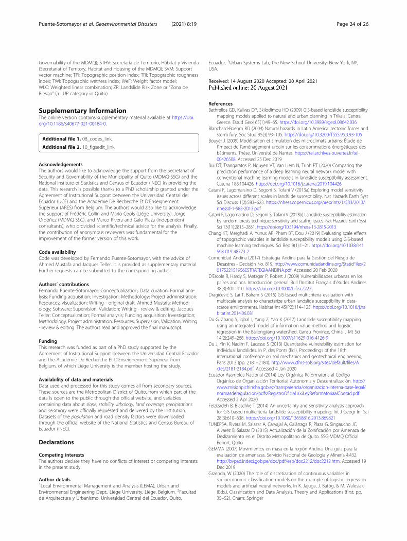
Governability of the MDMQ); STHV: Secretaría de Territorio, Hábitat y Vivienda(Secretariat of Territory, Habitat and Housing of the MDMQ); SVM: Supportvector machine; TPI: Topographic position index; TRI: Topographic roughnessindex; TWI: Topographic wetness index; WeF: Weight factor model;WLC: Weighted linear combination; ZR: Landslide Risk Zone or “Zona deRiesgo” (a LUP category in Quito)

Supplementary InformationThe online version contains supplementary material available at https://doi.org/10.1186/s40677-021-00184-0.

Additional file 1. 08_codes_link.

Additional file 2. 10_figsedit_link.

AcknowledgementsThe authors would like to acknowledge the support from the Secretariat ofSecurity and Governability of the Municipality of Quito (MDMQ-SSG) and theNational Institute of Statistics and Census of Ecuador (INEC) in providing thedata. This research is possible thanks to a PhD scholarship granted under theAgreement of Institutional Support between the Universidad Central delEcuador (UCE) and the Académie De Recherche Et D’EnseignementSupérieur (ARES) from Belgium. The authors would also like to acknowledgethe support of Frédéric Collin and Mario Cools (Liège University), JorgeOrdóñez (MDMQ-SSG), and Marco Rivera and Galo Plaza (independentconsultants), who provided scientific/technical advice for the analysis. Finally,the contribution of anonymous reviewers was fundamental for theimprovement of the former version of this work.

Code availabilityCode was developed by Fernando Puente-Sotomayor, with the advice ofAhmed Mustafa and Jacques Teller. It is provided as supplementary material.Further requests can be submitted to the corresponding author.

Authors’ contributionsFernando Puente-Sotomayor: Conceptualization; Data curation; Formal ana-lysis; Funding acquisition; Investigation; Methodology; Project administration;Resources; Visualization; Writing - original draft. Ahmed Mustafa: Method-ology; Software; Supervision; Validation; Writing - review & editing. JacquesTeller: Conceptualization; Formal analysis; Funding acquisition; Investigation;Methodology; Project administration; Resources; Supervision; Validation; Writing- review & editing. The authors read and approved the final manuscript.

FundingThis research was funded as part of a PhD study supported by theAgreement of Institutional Support between the Universidad Central Ecuadorand the Académie De Recherche Et D’Enseignement Supérieur fromBelgium, of which Liège University is the member hosting the study.

Availability of data and materialsData used and processed for this study comes all from secondary sources.These sources are the Metropolitan District of Quito, from which part of thedata is open to the public through the official website, and variablescontaining data about slope, stability, lithology, land coverage, precipitationsand seismicity were officially requested and delivered by the institution.Datasets of the population and road density factors were downloadedthrough the official website of the National Statistics and Census Bureau ofEcuador (INEC).

Declarations

Competing interestsThe authors declare they have no conflicts of interest or competing interestsin the present study.

Author details1Local Environmental Management and Analysis (LEMA), Urban andEnvironmental Engineering Dept., Liège University, Liège, Belgium. 2Facultadde Arquitectura y Urbanismo, Universidad Central del Ecuador, Quito,

Ecuador. 3Urban Systems Lab, The New School University, New York, NY,USA.

Received: 14 August 2020 Accepted: 20 April 2021

ReferencesBathrellos GD, Kalivas DP, Skilodimou HD (2009) GIS-based landslide susceptibility

mapping models applied to natural and urban planning in Trikala, CentralGreece. Estud Geol 65(1):49–65. https://doi.org/10.3989/egeol.08642.036

Blanchard-Boehm RD (2004) Natural hazards in Latin America: tectonic forces andstorm fury. Soc Stud 95(3):93–105. https://doi.org/10.3200/TSSS.95.3.93-105

Bouyer J (2009) Modélisation et simulation des microclimats urbains: Étude del’impact de l’aménagement urbain sur les consommations énergétiques desbâtiments. Thèse, Université de Nantes. https://tel.archives-ouvertes.fr/tel-00426508. Accessed 25 Dec 2019

Bui DT, Tsangaratos P, Nguyen VT, Van Liem N, Trinh PT (2020) Comparing theprediction performance of a deep learning neural network model withconventional machine learning models in landslide susceptibility assessment.Catena 188:104426. https://doi.org/10.1016/j.catena.2019.104426

Catani F, Lagomarsino D, Segoni S, Tofani V (2013a) Exploring model sensitivityissues across different scales in landslide susceptibility. Nat Hazards Earth SystSci Discuss 1(2):583–623. https://nhess.copernicus.org/preprints/1/583/2013/nhessd-1-583-2013.pdf

Catani F, Lagomarsino D, Segoni S, Tofani V (2013b) Landslide susceptibility estimationby random forests technique: sensitivity and scaling issues. Nat Hazards Earth SystSci 13(11):2815–2831. https://doi.org/10.5194/nhess-13-2815-2013

Chang KT, Merghadi A, Yunus AP, Pham BT, Dou J (2019) Evaluating scale effectsof topographic variables in landslide susceptibility models using GIS-basedmachine learning techniques. Sci Rep 9(1):1–21. https://doi.org/10.1038/s41598-019-48773-2

Comunidad Andina (2017) Estrategia Andina para la Gestión del Riesgo deDesastres - Decisión No. 819. http://www.comunidadandina.org/StaticFiles/2017522151956ESTRATEGIAANDINA.pdf. Accessed 20 Feb 2020

D’Ercole R, Hardy S, Metzger P, Robert J (2009) Vulnerabilidades urbanas en lospaíses andinos. Introducción general. Bull l’Institut Français d’études Andines38(3):401–410. https://doi.org/10.4000/bifea.2222

Dragićević S, Lai T, Balram S (2015) GIS-based multicriteria evaluation withmultiscale analysis to characterize urban landslide susceptibility in data-scarce environments. Habitat Int 45(P2):114–125. https://doi.org/10.1016/j.habitatint.2014.06.031

Du G, Zhang Y, Iqbal J, Yang Z, Yao X (2017) Landslide susceptibility mappingusing an integrated model of information value method and logisticregression in the Bailongjiang watershed, Gansu Province, China. J Mt Sci14(2):249–268. https://doi.org/10.1007/s11629-016-4126-9

Du J, Yin K, Nadim F, Lacasse S (2013) Quantitative vulnerability estimation forindividual landslides. In P. des Ponts (Ed.), Proceedings of the 18thinternational conference on soil mechanics and geotechnical engineering,Paris 2013 (pp. 2181–2184). http://www.cfms-sols.org/sites/default/files/Actes/2181-2184.pdf. Accessed 4 Jan 2020

Ecuador Asamblea Nacional (2014) Ley Orgánica Reformatoria al CódigoOrgánico de Organización Territorial, Autonomía y Descentralización. http://www.misionpichincha.gob.ec/transparencia/organizacion-interna-base-legal/normasderegulacion/pdfs/RegistroOficial166LeyReformatoriaalCootad.pdf.Accessed 2 Apr 2020

Feizizadeh B, Blaschke T (2014) An uncertainty and sensitivity analysis approachfor GIS-based multicriteria landslide susceptibility mapping. Int J Geogr Inf Sci28(3):610–638. https://doi.org/10.1080/13658816.2013.869821

FUNEPSA, Rivera M, Salazar A, Carvajal A, Galárraga R, Plaza G, Singaucho JC,Álvarez B, Salazar D (2015) Actualización de la Zonificación por Amenaza deDeslizamiento en el Distrito Metropolitano de Quito. SSG-MDMQ OfficialReport, Quito

GEMMA (2007) Movimientos en masa en la región Andina: Una guía para laevaluación de amenazas. Servicio Nacional de Geología y Minería 4:432.http://bvpad.indeci.gob.pe/doc/pdf/esp/doc2212/doc2212.htm. Accessed 19Dec 2019

Grzenda, W (2020) The role of discretization of continuous variables insocioeconomic classification models on the example of logistic regressionmodels and artificial neural networks. In K. Jajuga, J. Batóg, & M. Walesiak(Eds.), Classification and Data Analysis. Theory and Applications (first, pp.35–52). Cham: Springer


https://doi.org/10.1186/s40677-021-00184-0

https://doi.org/10.1186/s40677-021-00184-0

https://doi.org/10.3989/egeol.08642.036

https://doi.org/10.3200/TSSS.95.3.93-105

https://tel.archives-ouvertes.fr/tel-00426508

https://tel.archives-ouvertes.fr/tel-00426508

https://doi.org/10.1016/j.catena.2019.104426

https://nhess.copernicus.org/preprints/1/583/2013/nhessd-1-583-2013.pdf

https://nhess.copernicus.org/preprints/1/583/2013/nhessd-1-583-2013.pdf

https://doi.org/10.5194/nhess-13-2815-2013

https://doi.org/10.1038/s41598-019-48773-2

https://doi.org/10.1038/s41598-019-48773-2

http://www.comunidadandina.org/StaticFiles/2017522151956ESTRATEGIAANDINA.pdf

http://www.comunidadandina.org/StaticFiles/2017522151956ESTRATEGIAANDINA.pdf

https://doi.org/10.4000/bifea.2222

https://doi.org/10.1016/j.habitatint.2014.06.031


https://doi.org/10.1007/s11629-016-4126-9

http://www.cfms-sols.org/sites/default/files/Actes/2181-2184.pdf

http://www.cfms-sols.org/sites/default/files/Actes/2181-2184.pdf

http://www.misionpichincha.gob.ec/transparencia/organizacion-interna-base-legal/normasderegulacion/pdfs/RegistroOficial166LeyReformatoriaalCootad.pdf



https://doi.org/10.1080/13658816.2013.869821

http://bvpad.indeci.gob.pe/doc/pdf/esp/doc2212/doc2212.htm

Gudiyangada Nachappa T, Kienberger S, Meena SR, Hölbling D, Blaschke T (2020)Comparison and validation of per-pixel and object-based approaches forlandslide susceptibility mapping. Geomatics Nat Hazards Risk 11(1):572–600.https://doi.org/10.1080/19475705.2020.1736190

Hemasinghe H, Rangali RSS, Deshapriya NL, Samarakoon L (2018) Landslidesusceptibility mapping using logistic regression model (a case study inBadulla District, Sri Lanka). Proc Eng 212:1046–1053. https://doi.org/10.1016/j.proeng.2018.01.135

Highland LM, Bobrowsky P (2008) The Landslide Handbook — A Guide toUnderstanding Landslides. US Geological Survey Circular 1325, Reston.https://pubs.usgs.gov/circ/1325/pdf/C1325_508.pdf. Accessed 12 Nov 2019

INEC (2016) Proyeccion Cantonal Total 2010–2020. INEC Registry. http://www.inec.gob.ec/estadisticas/index.php?option=com_content&view=article&id=329&Itemid=328&lang=es. Accessed 12 Nov 2019

Inostroza L (2017) Informal urban development in Latin American urban peripheries.Spatial assessment in Bogota, Lima and Santiago de Chile. Landscape UrbanPlan 165(1):267–279. https://doi.org/10.1016/j.landurbplan.2016.03.021

Kaynia AM, Papathoma-Köhle M, Neuhäuser B, Ratzinger K, Wenzel H, Medina-Cetina Z (2008) Probabilistic assessment of vulnerability to landslide:application to the village of Lichtenstein, Baden-Württemberg, Germany. EngGeol 101(1–2):33–48. https://doi.org/10.1016/j.enggeo.2008.03.008

Kirschbaum D, Stanley T (2018) Satellite-based assessment of rainfall-triggeredlandslide Hazard for situational awareness. Earth’s Future 6(3):505–23. https://doi.org/10.1002/2017EF00071

Klimeš J, Rios Escobar V (2010) A landslide susceptibility assessment in urbanareas based on existing data: an example from the Iguaná Valley, MedellínCity, Colombia. Natural Hazards Earth Syst Sci 10(10):2067–2079. https://doi.org/10.5194/nhess-10-2067-2010

Lara M, Sepúlveda SA, Celis C, Rebolledo S, Ceballos P (2018) Landslidesusceptibility maps of Santiago city, Andean foothills, Chile. Andean Geol45(3):433–442. https://doi.org/10.5027/andgeoV45n3-3151

Lee S, Baek WK, Jung HS, Lee S (2020) Susceptibility mapping on urbanlandslides using deep learning approaches in mt. Umyeon. Appl Sci 10(22):1–18. https://doi.org/10.3390/app10228189

Leoni G, Barchiesi F, Catallo F, Dramis F, Fubelli G, Lucifora S, Mattei M, Pezzo G,Puglisi C (2009) GIS methodology to assess landslide susceptibility:application to a river catchment of Central Italy. J Maps 5(1):87–93.https://doi.org/10.4113/jom.2009.1041

Lombardo L, Mai PM (2018) Presenting logistic regression-based landslide susceptibilityresults. Eng Geol 244(January):14–24. https://doi.org/10.1016/j.enggeo.2018.07.019

Meena SR, Ghorbanzadeh O, Blaschke T (2019) A comparative study of statistics-based landslide susceptibility models: a case study of the region affected bythe Gorkha earthquake in Nepal. ISPRS Int J Geo Inf 8(2). https://doi.org/10.3390/ijgi8020094

Melchiorre C, Castellanos Abella EA, van Westen CJ, Matteucci M (2011)Evaluation of prediction capability, robustness, and sensitivity in non-linearlandslide susceptibility models, Guantánamo, Cuba. Comput Geosci 37(4):410–425. https://doi.org/10.1016/j.cageo.2010.10.004

Norman G (2010) Likert scales, levels of measurement and the “laws” of statistics.Adv Health Sci Educ 15(5):625–632. https://doi.org/10.1007/s10459-010-9222-y

Orán Cáceres JP, Gómez Delgado M, Bosque Sendra J (2010) Una propuestacomplementaria de análisis de sensibilidad de un modelo basado entécnicas sig y evaluación multicriterio. Pubs. Univ. de Sevilla. 2010(14):971–987. http://hdl.handle.net/11441/66681. Accessed 21 Nov 2019

Pascale S, Parisi S, Mancini A, Schiattarella M, Conforti M, Sole A, MurganteB, Sdao F (2013) Landslide susceptibility mapping using artificial neuralnetwork in the urban area of Senise and San Costantino Albanese(Basilicata, southern Italy). In: Murgante B. et al. (eds) ComputationalScience and Its Applications. ICCSA 2013. Lecture Notes in ComputerScience. Springer, Berlin, Heidelberg (pp. 473–488). https://doi.org/10.1007/978-3-642-39649-6_34

Pasta DJ (2009) Learning when to be discrete: continuous vs. categoricalpredictors. In: SAS Global Forum 2009, Statistics and Data Analysis. 2009 Mar(p. 248). https://support.sas.com/resources/papers/proceedings09/248-2009.pdf. Accessed 19 Nov 2019

Pawluszek K, Borkowski A, Tarolli P (2018) Sensitivity analysis of automaticlandslide mapping: numerical experiments towards the best solution.Landslides 15(9):1851–1865. https://doi.org/10.1007/s10346-018-0986-0

Poelmans L, Van Rompaey A (2010) Complexity and performance of urbanexpansion models. Comput Environ Urban Syst 34(1):17–27. https://doi.org/10.1016/j.compenvurbsys.2009.06.001

Puente-Sotomayor F, Egas A, Teller J (2021) Land policies for landslide riskreduction in Andean cities. Habitat International 107(Jan):102298. https://doi.org/10.1016/j.habitatint.2020.102298

Puente-Sotomayor F, Villamarin P, Cevallos A (2018) Riesgos de deslizamiento enQuito, ¿funciona la política? In: Asociación Geográfica del Ecuador (ed)Territorios en transición: Transformaciones de la Geografía del Ecuador en elsiglo XXI - Memorias del 1er Congreso Nacional de Geografía del Ecuador.Asociación Geográfica del Ecuador, Quito, pp 1–15. https://congresonacionalagec.files.wordpress.com/2018/02/memoria_cng_2018.pdf. Accessed 15 Dec2019.

Psomiadis E, Papazachariou A, Soulis KX, Alexiou DS, Charalampopoulos I (2020)Landslide mapping and susceptibility assessment using geospatial analysisand earth observation data. Land 9(5):133. https://doi.org/10.3390/land9050133.

Quito Alcaldia del Distrito Metropolitano (2018) Resolución Administrativa A008,Ordenanzas y Resoluciones 1–5 (2018). http://www7.quito.gob.ec/mdmq_ordenanzas/Resoluciones de Alcaldía/Año 2018/RA-2018-008-DIRECCIONMETROPOLITANA DE RESILIENCIACREACION.PDF. Accessed 20 Feb 2020

Quito Concejo del Distrito Metropolitano (2003) Ordenanza Metropolitana No.095 Régimen de Suelo. http://www7.quito.gob.ec/mdmq_ordenanzas/Ordenanzas/ORDENANZAS AÑOS ANTERIORES/ORDM-095 - NUEVO REGIMENDELSUELO.pdf. Accessed 15 Dec 2019

Quito Concejo del Distrito Metropolitano (2011) Ordenanza Metropolitana No.172 Régimen de Suelo de Quito. http://www7.quito.gob.ec/mdmq_ordenanzas/ConcejoAbierto/Ordenanzas/ORDENANZASMUNICIPALES/MUNICIPAL(172)/MUNICIPAL_0172_517.pdf. Accessed 4 Jan 2020.

Quito Municipio del Distrito Metropolitano (2015) Plan de Desarrollo yOrdenamiento Territorial 2015 - Diagnóstico Eje Territorial. MDMQ. http://www7.quito.gob.ec/mdmq_ordenanzas/Sesiones del Concejo/2015/SesiónExtraordinaria 2015-02-13/PMDOT 2015-2025/Volumen I/6. DiagnósticoTerritorial.pdf. Accessed 12 Nov 2019

Quito Municipio del Distrito Metropolitano (2017) Estrategia de ResilienciaDistrito Metropolitano de Quito. MDMQ. http://www.pichincha.gob.ec/pichincha/cantones/item/23-distrito-metropolitano-de-quito.html. Accessed21 Nov 2019

Ramos-Bernal RN, Vázquez-Jiménez R, Sánchez Tizapa S, Arroyo Matus R (2019)Characterization of susceptible landslide zones by an accumulated index. In R.Ram & M. Lazzari (Eds.), Landslides - Investigation and Monitoring (first, pp. 1–26). Intech Open. https://www.intechopen.com/books/advanced-biometric-technologies/liveness-detection-in-biometrics. Accessed 12 Feb 2020

Rebotier J (2016) El Riesgo y su Gestión en Ecuador - Una Mirada de GeografíaSocial y Política. Centro de Publicaciones Pontificia Universidad Católica delEcuador, Quito. https://biblio.flacsoandes.edu.ec/shared/biblio_view.php?bibid=143165&tab=opac. Accessed 15 May 2018.

Reichenbach P, Rossi M, Malamud BD, Mihir M, Guzzetti F (2018) A review ofstatistically-based landslide susceptibility models. Earth Sci Rev 180(March):60–91. https://doi.org/10.1016/j.earscirev.2018.03.001

Ronchetti F, Corsini A, Kollarits S, Leber D, Papez J, Plunger K, Preseren T,Schnetzer I, Stefani M (2013) Improve information provision for disastermanagement: MONITOR II, EU project. In: Margottini C, Canuti P, Sassa K(eds) Landslide science and practice, Social and Economic Impact andPolicies, vol 7. Springer, Rome, pp 47–54. https://doi.org/10.1007/978-3-642-31313-4_7

Saltelli A, Aleksankina K, Becker W, Fennell P, Ferretti F, Holst N, Li S, Wu Q (2019)Why so many published sensitivity analyses are false: a systematic review ofsensitivity analysis practices. Environ Model Softw, 114(2019):29–39. https://doi.org/10.1016/j.envsoft.2019.01.012

Shahabi H, Hashim M (2015) Landslide susceptibility mapping using GIS-basedstatistical models and remote sensing data in tropical environment. Sci Rep5:1–15. https://doi.org/10.1038/srep09899

Shahri AA, Spross J, Johansson F, Larsson S (2019) Landslide susceptibility hazardmap in Southwest Sweden using artificial neural network. Catena 183(2019):104225. https://doi.org/10.1016/j.catena.2019.104225

Sepúlveda SA, Petley DN (2015) Regional trends and controlling factors of fatallandslides in Latin America and the Caribbean. Nat Hazards Earth Syst Sci15(8):1821–1833. https://doi.org/10.5194/nhess-15-1821-2015

Sîrbu F, Drăguț L, Oguchi T, Hayakawa Y, Micu M (2019) Scaling land-surfacevariables for landslide detection. Progress Earth Planet Sci 6(1):1–13. https://doi.org/10.1186/s40645-019-0290-1

UNISDR (2018) UNISDR annual report 2017. UNISDR, Geneva. https://www.unisdr.org/files/58158_unisdr2017annualreport.pdf. Accessed 12 Nov 2019.


https://doi.org/10.1080/19475705.2020.1736190

https://doi.org/10.1016/j.proeng.2018.01.135

https://doi.org/10.1016/j.proeng.2018.01.135

https://pubs.usgs.gov/circ/1325/pdf/C1325_508.pdf

http://www.inec.gob.ec/estadisticas/index.php?option=com_content&view=article&id=329&Itemid=328&lang=es



https://doi.org/10.1016/j.landurbplan.2016.03.021

https://doi.org/10.1016/j.enggeo.2008.03.008

https://doi.org/10.1002/2017EF00071

https://doi.org/10.1002/2017EF00071



https://doi.org/10.5027/andgeoV45n3-3151

https://doi.org/10.3390/app10228189

https://doi.org/10.4113/jom.2009.1041

https://doi.org/10.1016/j.enggeo.2018.07.019

https://doi.org/10.3390/ijgi8020094

https://doi.org/10.3390/ijgi8020094

https://doi.org/10.1016/j.cageo.2010.10.004

https://doi.org/10.1007/s10459-010-9222-y

http://hdl.handle.net/11441/66681

https://doi.org/10.1007/978-3-642-39649-6_34

https://doi.org/10.1007/978-3-642-39649-6_34

https://support.sas.com/resources/papers/proceedings09/248-2009.pdf

https://support.sas.com/resources/papers/proceedings09/248-2009.pdf

https://doi.org/10.1007/s10346-018-0986-0

https://doi.org/10.1016/j.compenvurbsys.2009.06.001

https://doi.org/10.1016/j.compenvurbsys.2009.06.001

https://doi.org/10.1016/j.habitatint.2020.102298

https://doi.org/10.1016/j.habitatint.2020.102298

https://congresonacionalagec.files.wordpress.com/2018/02/memoria_cng_2018.pdf

https://congresonacionalagec.files.wordpress.com/2018/02/memoria_cng_2018.pdf

https://doi.org/10.3390/land9050133

https://doi.org/10.3390/land9050133

http://www7.quito.gob.ec/mdmq_ordenanzas/Resoluciones

http://www7.quito.gob.ec/mdmq_ordenanzas/Resoluciones

http://www7.quito.gob.ec/mdmq_ordenanzas/Ordenanzas/ORDENANZAS

http://www7.quito.gob.ec/mdmq_ordenanzas/Ordenanzas/ORDENANZAS

http://www7.quito.gob.ec/mdmq_ordenanzas/ConcejoAbierto/Ordenanzas/ORDENANZASMUNICIPALES/MUNICIPAL(172)/MUNICIPAL_0172_517.pdf



http://www7.quito.gob.ec/mdmq_ordenanzas/Sesiones

http://www7.quito.gob.ec/mdmq_ordenanzas/Sesiones

http://www.pichincha.gob.ec/pichincha/cantones/item/23-distrito-metropolitano-de-quito.html

http://www.pichincha.gob.ec/pichincha/cantones/item/23-distrito-metropolitano-de-quito.html

https://www.intechopen.com/books/advanced-biometric-technologies/liveness-detection-in-biometrics

https://www.intechopen.com/books/advanced-biometric-technologies/liveness-detection-in-biometrics

https://biblio.flacsoandes.edu.ec/shared/biblio_view.php?bibid=143165&tab=opac

https://biblio.flacsoandes.edu.ec/shared/biblio_view.php?bibid=143165&tab=opac

https://doi.org/10.1016/j.earscirev.2018.03.001

https://doi.org/10.1007/978-3-642-31313-4_7

https://doi.org/10.1007/978-3-642-31313-4_7

https://doi.org/10.1016/j.envsoft.2019.01.012

https://doi.org/10.1016/j.envsoft.2019.01.012

https://doi.org/10.1038/srep09899



https://doi.org/10.1186/s40645-019-0290-1

https://doi.org/10.1186/s40645-019-0290-1

https://www.unisdr.org/files/58158_unisdr2017annualreport.pdf

https://www.unisdr.org/files/58158_unisdr2017annualreport.pdf

USGS (2004) Landslide Types and Processes. Highway Research Board SpecialReport. U.S. Department of the Interior, U.S. Geological Survey. https://pubs.usgs.gov/fs/2004/3072/pdf/fs2004-3072.pdf. Accessed 21 Nov 2019.

van Dessel W, van Rompaey A, Szilassi P (2011) Sensitivity analysis of logisticregression parameterization for land use and land cover probabilityestimation. Int J Geogr Inf Sci 25(3):489–508. https://doi.org/10.1080/13658810903194256

van Lindert P (2016) Rethinking urban development in Latin America: a review ofchanging paradigms and policies. Habitat Int 54:253–264. https://doi.org/10.1016/j.habitatint.2015.11.017

Wang Y, Feng L, Li S, Ren F, Du Q (2020) A hybrid model considering spatialheterogeneity for landslide susceptibility mapping in Zhejiang Province,China. Catena 188(July 2019):104425. https://doi.org/10.1016/j.catena.2019.104425

Williams R (2019) Ordinal independent variables. Notre Dame. https://www3.nd.edu/~rwilliam/xsoc73994/OrdinalIndependent.pdf. Accessed 21 Nov 2019.

Wubalem A (2020) Modeling of landslide susceptibility in a part of Abay Basin,northwestern Ethiopia. Open Geosciences 12(1):1440–1467. https://doi.org/10.1515/geo-2020-0206

Zhang L, Ray H, Priestley J, Tan S (2020) A descriptive study of variable discretizationand cost-sensitive logistic regression on imbalanced credit data. J Appl Stat47(3):568–581. https://doi.org/10.1080/02664763.2019.1643829

Publisher’s NoteSpringer Nature remains neutral with regard to jurisdictional claims inpublished maps and institutional affiliations.


https://pubs.usgs.gov/fs/2004/3072/pdf/fs2004-3072.pdf

https://pubs.usgs.gov/fs/2004/3072/pdf/fs2004-3072.pdf

https://doi.org/10.1080/13658810903194256

https://doi.org/10.1080/13658810903194256





https://www3.nd.edu/%7erwilliam/xsoc73994/OrdinalIndependent.pdf

https://www3.nd.edu/%7erwilliam/xsoc73994/OrdinalIndependent.pdf

https://doi.org/10.1515/geo-2020-0206

https://doi.org/10.1515/geo-2020-0206

https://doi.org/10.1080/02664763.2019.1643829

Documents

Landslide Susceptibility Mapping of Urban Areas: Logistic