THE LANGUAGE OF PARTICLE SIZE As published in GXP, Spring 2011 (Vol15/No2)

Rebecca Lea Wolfrom

KEY POINTS The following key points are discussed:

• Knowledge and understanding of particle size data are vital to practitioners in the pharmaceutical, mining,

environmental, paints and coatings, and other industries.

• The vocabulary of particle size is unique and complex. Clear understanding of terminology is necessary

for correct interpretation of data.

• Graphical representation of particle size distributions by histogram and / or cumulative distributions is

fundamental. Distributions may also be expressed by various percentile notations.

• Laser light scattering and other instrumentation report particle size distribution data in terms of equivalent

spherical diameter.

• Data from various instruments may be expressed as a number distribution or a volume distribution.

• A listing of relevant particle size terminology and definitions is provided.

• Important details associated with the interpretation and understanding of particle size data are discussed.

• Correct interpretation of particle size analyses is rooted in an understanding of distributions and the

associated statistical descriptive terminology.

INTRODUCTION Most practitioners in the pharmaceutical, mining, environmental, paints and coatings, and other fields have

reason to know the sizes of particles in a given powder or slurry sample. While many technologies exist to

describe that collection of sizes, the reports delivered by those technologies are written in their own

vocabulary. This particle size lexicon can convey a tremendous amount of information as long as the terms

and their definitions are clearly understood and their underlying assumptions are fully considered. This

discussion introduces the common values encountered on a typical particle size report and provides references

for deeper mathematical interpretations. With this information in hand, the reader will be well-equipped to

judge compliance.

THE PARTICLE SIZE DISTRIBUTION AND ITS REPRESENTATION A fundamental concept to understand is that any accumulation of particles larger than molecular scale actually

contains many different sizes of particles (1). Thus the term distribution is applied. In this way, it is

acknowledged that a collection of particulate contains a continuous range of sizes. A collection of particles

having a single size is only attainable with meticulous classification effort.

In order to represent the size range, a frequency diagram or histogram is typically produced. The histogram

is a bar graph wherein the x-axis represents the particle size.

The vertical height of the bars (the y-axis) represents the relative amount of matter contained at that size, or

the frequency of occurrences. ISO 9276-1:1998(E) (2) describes the plotting procedure in detail.

A sieve analysis demonstrates the concept. A free-flowing powder sample is introduced to the top of a stack

of six sieves having graduated mesh sizes, closed by a solid pan at the bottom. After completing the requisite

agitating methodology, some portion of the original sample rests on each sieve, with the finest portion falling

all the way through to the pan at the bottom. Hypothetically, the data could resemble Table I.

TABLE I. SIEVE RESULTS

Sieve Size

(Length Units)

Amount Retained on

Respective Sieve

(Weight Units)

Incremental Weight %

Retained

60 0 0/220 = 0%

50 5 5/220 ≈ 2%

40 30 30/220 ≈ 14%

30 150 150/220 ≈ 68%

20 30 30/220 ≈ 14%

10 5 5/220 ≈ 2%

Pan Trace 0/220 ≈ 0%

Sum = 220 Sum = 100%

The sieve sizes are plotted on the x-axis, while the calculated Incremental Weight % Retained on each sieve

governs the height of each bar (y-axis point). In this case, convention is to plot the height at the center of the

size bin, i.e. 68% weight between 30 length and 40 length, at 35 length units. Instrument software can often

be customized, however, so it is important to check the output settings. The Beckman Coulter laser

diffractors, for example, give the option to print data at the left, right, or center of the size bin. As a result,

this should be kept in mind when evaluating results with respect to Certificates of Analysis specifications, or

when cross-comparing two datasets from different labs.

The histogram for the Table I sieve dataset above follows in Figure 1.

0-10um10-20um

20-30um

30-40um

40-50um

50-60um60+ um

0

10

20

30

40

50

60

70

80

Sieve Sizes (Length Units)

Incre

men

tal W

t %

Reta

ined

FIGURE 1. Histogram based on Table I.

Note there exists an amount of material between two sieve sizes. This size range is called a size bin. Bins are

represented by the width of the bars in the histogram. In an instrumentation output, the size bins (or channels)

are typically predefined and numbered consecutively. Each detected occurrence is “filed” into the appropriate

section (3). The number of bins or channels in the output indicates the resolution of the instrument.

The size bins may be wide or narrow, depending on the resolution of the data. Increasing the resolution in

this example would be the equivalent of inserting more sieves into the stack. The overall size range remains

the same, but the number of data points collected within that range increases. As the number of data points

increases, the bins narrow smaller and smaller and the graph tends toward a smooth line. To obtain a graph

made up of only points on a smoothed line, calculate the Cumulative % Retained as in Table II. The resulting

Cumulative distribution is shown in Figure 2 (1).

TABLE II. SIEVE RESULTS, INCLUDING CUMULATIVE CALCULATIONS

Sieve Size

(Length Units)

Amount Retained

(Weight Units)

Incremental

Weight %

Retained

Cumulative

Weight %

Retained

Cumulative

Weight % Passing

60 Trace 0/220 = 0% 0 100-0 = 100%

50 5 5/220 ≈ 2% 0+2 = 2% 100-2 = 98%

40 30 30/220 ≈ 14% 2+14 = 16% 100-16 = 84%

30 150 150/220 ≈ 68% 16+68 = 84% 100-84 = 16%

20 30 30/220 ≈ 14% 84+14 = 98% 100-98 = 2%

10 5 5/220 ≈ 2% 98+2 = 100% 100-100 = 0%

Pan Trace 0/220 = 0% 100+0 = 100% 100-100 = 0%

Sum = 220 Sum = 100%

0.0

10.0

20.0

30.0

40.0

50.0

60.0

0 10 20 30 40 50 60 70

Sieve Sizes (Length Units)

Cu

mu

lati

ve W

eig

ht

% P

assin

g

FIGURE 2. Continuous Cumulative Curve.

In order to convert a cumulative curve back to a continuous incremental distribution, take the derivative of the

cumulative curve with respect to size (2). Figure 3 shows the result of this process, including higher

resolution. Here, the bins are aligned at the left-hand side with each x-axis value.

FIGURE 3. Continuous Incremental Distribution: Derivative of the Cumulative Distribution.

Reviewing Figures 1-3 shows that all data have been plotted on linear x-axes. Some readers may have

encountered particle size data plotted with the x-axis on a log scale. The log scale adds convenience for

several reasons. According to Brittain, applying a log scale to the x-axis helps to convert leaning or skewed

linear histograms into a more normal or Gaussian shape (1). Also, the equal distance spacing between size

bins on a linear scale can produce cumbersome graphical representations of the widely distributed data often

encountered in particle size measurements. Use of a log scale thus manageably compacts the data

presentation (2).

EMBEDDED MEANING IN THE NOTATION Particle size reports use notation specific to the field that may not be intuitive. The following are common

terminologies associated with particle size data presentation.

Percentiles are of utmost importance. The shorthand is usually written as ‘d’ or ‘x’ with a subscripted number

referring to a percent. For example, d50 or x50 refers to the 50th percentile, meaning the diameter of a sphere

at which 50% of the particles in the sample are smaller. ISO 9276-1:1998(E) (2) specifically indicates that d

is interchangeable with x. Other terminology for the same value is D(v, 0.5). The v represents a volume

weighted basis, in this example.

Similarly, d10 = x10 = the 10th percentile = the diameter of a sphere at which 10% of the particles in the

sample are smaller; on a volume basis = D(v, 0.1), and so on.

Other details in the notation can change as well. D(n,0.1) = the diameter of a sphere at which 10% of the

particles in the samples are smaller on a number basis. The ‘n’ indicates the basis.

Sieve Sizes (Length Units)

Incre

men

tal

Wt

% R

eta

ined

Most instruments default to a percent smaller (or “<” or “less than”) basis. However, this can be typically

changed by the operator depending upon the desired output. Keep this in mind when evaluating results for

comparison to specifications or other datasets.

EQUIVALENT SPHERICAL DIAMETER Particle size results from an assortment of instruments are reported in the form of a histogram. However, the

graphs are developed more indirectly than the direct weighing technique described earlier in the sieve

example. A very commonly used output is that of laser light scattering (laser diffraction). This technique,

along with numerous others described in detail by Allen (4), defaults to reporting in terms of Equivalent

Spherical Diameter [or Volume Weighted Equivalent Spherical Diameter for laser diffractors]. This phrase

is critically important to assess the possible subtleties underlying a particle size measurement result.

Equivalent spherical diameter is defined by ISO 9276-1:1998(E) (2) as the diameter of a sphere having the

same physical properties as the particle under examination. Some examples of such physical properties (5)

include the following: Particles reported using this assumption will

• Particles reported using this assumption will pass through the same sized aperture as the equivalent sphere

(sieving)

• Will settle at the same velocity as the equivalent sphere (sedimentation)

• Will scatter light at the same intensity at the same angle as the equivalent sphere (laser diffraction)

• Will displace the same volume of liquid as the equivalent sphere (electrosensing zone).

The reason the concept is so common in the field is due to the extreme programming requirements of the

electronics used and the extensive dataset that would be generated if information could be collected on all

possible dimensions. Visually, the human eye can distinguish several dimensions within a single irregularly-

shaped particle (see the diagrams by Brittain [1]). However, the end user is expecting a “short answer.” How

can a rod, for example, with one long axis and one short axis, or even corner-to-corner within the rod, be

defined in a single number?

The custom is to describe a singular feature of the particle which can be mathematically converted back to the

dimensions of a sphere, the only three-dimensional shape which has truly one measurement in all directions—

its diameter (d). Some such singular features are weight, surface area, or volume of the rod. Each can be

described with one value regardless of how different the axes are from each other. As such, the volume (for

example) of a rod (or cylinder) is

hrVrod

2π=

where r is the radius of the end circle (r is half of the circle’s diameter, or d/2), h is the height of the rod, and

V is the volume. Instead of needing to know how wide and high the rod is, one can simply determine V (say

33.5 µm3), then equate that to the volume of a sphere

rodsphere Vd

V =

=

3

23

4π

By doing so, one eliminates the two variables r and h, and obtains a single value for the diameter (d = 4 µm in

this example). This diameter is that of a sphere having the same volume as the original rod, which had

several different linear dimensions. The programming and reporting becomes far more manageable. Rawle

(6) thoroughly describes the concept and all its implications in his technical paper.

The primary message to take away is to know something about the shape of the measured particulate. This

will help with interpretations of the measurement technique results and their effect on the detected size.

Shape information is usually evaluated using a microscope or by image analysis.

The National Institute of Standards and Technology (NIST) gives an exhaustive list of definitions of

diameters delivered by different measurement techniques (7). The differences are subtle but important in data

interpretation. An example is that the flow paths the particles follow during certain analyses will tend to align

elongated particles, thereby presenting only maximum dimensions to the detectors (which normally assume

tumbling in random orientation). This can bias the results large when considering the back-calculation to

equivalent spherical diameter.

NUMBER DISTRIBUTIONS VS. VOLUME DISTRIBUTIONS AND OTHERS The sieve example at the beginning of the article reported results in terms of weight. This directly-measured

reporting basis, however, is uncommon for most modern analysis techniques. The frequently encountered

terminology is either volume basis or number basis. Laser light scattering (laser diffraction) defaults to a

volume reporting structure, as does sedimentation. A histogram produced in this way reads as “x% of the

particles at the detected size occupy this much volume.” The histograms typically resemble a bell-shaped

(normal or Gaussian) curve in which a majority of the volume is occupied by the mid-range sized particles. It

may be difficult to conceptualize, but it has become standard language due to the direct output of the

instruments.

Laser diffraction, sedimentation, and several other forms of particle sizing techniques do not count or assign

size to individual particles. These techniques look at a measured property via a cloud or assemblage of

particles, and are thus termed “ensemble analyzers.”

Other techniques such as electro-sensing zone (Coulter) and light obscuration are designed to truly count

particles one by one and report the size of each. In this way, an actual number distribution is developed. A

typical number distribution genuinely shows the huge amount of fines present in the system, and it often

grows exponentially to be cut off by the y-axis at the technique’s lower detection limit. This is important to

note when evaluating data. An abrupt end to a distribution does not typically indicate an absence of

particulate below or above the designated size (unless, for example, it has been sieved) but generally indicates

a detection limit of the instrument or technique.

Computerized instruments are programmed to convert from their base outputs (microscope = number, laser

diffraction = volume) to the other presentation formats as detailed mathematically by Stintz (8). These

conversions should be regarded with caution, as the exponents in the equations are also applied to the inherent

error in the measurements, multiplying the error quickly (9).

To visualize a practical example of the difference between a number-based distribution and a volume-based

one, start by imagining a fruit basket. Only one huge juicy watermelon will fit in it, but plenty of small round

grapes can nestle into the nooks and crannies. The number distribution counts far more grapes (fines) than

watermelons (coarse), but the volume distribution clearly shows that the watermelon occupies far more space

than the entire collection of grapes that are scattered around, fitting in where possible. Giving these fruits

some dimensions, it can be said it only takes a single particle of 100-micron diameter to occupy the same

space as one million particles of 1-micron diameter!

33 )1(000,000,1)100(1 mm µµ ×=×

On a volume-based distribution, the coarse particulate volume far overshadows that of the fines in a normally

distributed sample, so the fines can easily be overlooked. A particle counter, which provides a number-based

distribution, will report the true story if fines are of critical import. Once again, this concept is of vital

importance when setting specifications, interpreting data, or investigating processing issues.

DEFINING TERMS GIVEN BY THE INSTRUMENT OUTPUTS The values above can be categorized in terms of their exponent: linear (first dimension or number) and cubic

(third dimension or volume.) Area would be square (second dimension.) These have great importance in

mathematically describing all typical terms reported by particle sizing instruments. A basic statistics text

could describe all of the following in terms of mathematical formulae.

The most basic terms describing the key points of a distribution curve are as follows:

• Mode – the most commonly occurring signal or size, also known as peak diameter.

• Median – the signal or size at which exactly half of the responses are below and half of the responses are above. On

a cumulative distribution, d50 is the median.

• Mean – the average.

A normal (or Gaussian) distribution has identical values for mode, median, and mean. It is also possible to find two

completely different shaped curves having the same values for mode, median, and mean.

Many different means can be calculated:

• Arithmetic Mean is the first dimension average, the one learned in grade school. It is the sum of all values

divided by the total number of values.

Arithmetic Mean n

xxx

n

xn

n

i

i +++==

∑= ...211

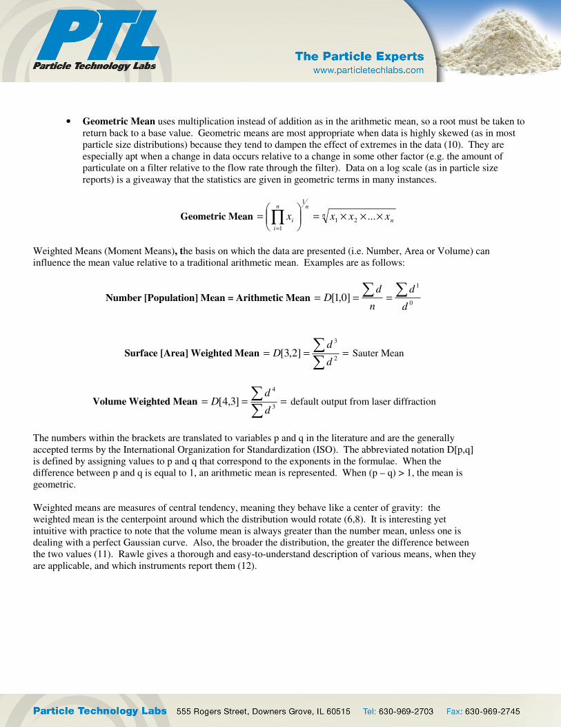
• Geometric Mean uses multiplication instead of addition as in the arithmetic mean, so a root must be taken to

return back to a base value. Geometric means are most appropriate when data is highly skewed (as in most

particle size distributions) because they tend to dampen the effect of extremes in the data (10). They are

especially apt when a change in data occurs relative to a change in some other factor (e.g. the amount of

particulate on a filter relative to the flow rate through the filter). Data on a log scale (as in particle size

reports) is a giveaway that the statistics are given in geometric terms in many instances.

Geometric Mean nn

nn

i

i xxxx ×××=

= ∏

=

...21

1

1

Weighted Means (Moment Means), the basis on which the data are presented (i.e. Number, Area or Volume) can

influence the mean value relative to a traditional arithmetic mean. Examples are as follows:

Number [Population] Mean = Arithmetic Mean 0

1

]0,1[d

d

n

dD

∑∑===

Surface [Area] Weighted Mean ===∑∑

2

3

]2,3[d

dD Sauter Mean

Volume Weighted Mean ===∑∑

3

4

]3,4[d

dD default output from laser diffraction

The numbers within the brackets are translated to variables p and q in the literature and are the generally

accepted terms by the International Organization for Standardization (ISO). The abbreviated notation D[p,q]

is defined by assigning values to p and q that correspond to the exponents in the formulae. When the

difference between p and q is equal to 1, an arithmetic mean is represented. When (p – q) > 1, the mean is

geometric.

Weighted means are measures of central tendency, meaning they behave like a center of gravity: the

weighted mean is the centerpoint around which the distribution would rotate (6,8). It is interesting yet

intuitive with practice to note that the volume mean is always greater than the number mean, unless one is

dealing with a perfect Gaussian curve. Also, the broader the distribution, the greater the difference between

the two values (11). Rawle gives a thorough and easy-to-understand description of various means, when they

are applicable, and which instruments report them (12).

The following are other definitions to describe the shape of the distribution curve:

• Standard Deviation – an indication of the spread of the curve about the mean.

• Variance – the square of the standard deviation; therefore also an indication of the spread of the data points. When

two factors act together to cause variability in a distribution, their standard deviation is a square root function.

Squaring it to obtain a value is therefore convenient in certain applications (13).

• Coefficient of Variation – another indication of the spread of the data, this one being normalized so it can be used to

compare datasets having very different means. Coefficient of variation is defined as the ratio of the standard

deviation to the mean. Sometimes the ratio is multiplied by 100 to report the coefficient as a percent; in any case the

value is always dimensionless. When reported as a percentage, it is commonly called the Percent Relative Standard

Deviation or %RSD.

• Skew (Skewness) – an indication of how far the distribution deviates from symmetry. A normal (Gaussian)

distribution has 0 skew. A distribution that “leans” to the right with a long tail at coarse sizes and with mean > mode

has positive skew, and the value will increase with increasing lean. A distribution that “leans” to the left with a long

tail at fine sizes and with mean < mode has negative skew (see Figure 4.)

Normal Distribution

Positive Skew

Negative Skew

FIGURE 4. Examples of Skew.

• Kurtosis – an indication of how sharply peaked the distribution plot is compared to a normal (Gaussian) distribution.

If the peak is very narrow and sharp with most particles having a size close to the mean, the distribution is leptokurtic

and the kurtosis is large. If the peak is broad, flat, and shaped like a plateau, the distribution is platykurtic and the

kurtosis is small (14) (see Figure 5).

Normal Distribution

Leptokurtic

Platykurtic

FIGURE 5. Examples of Kurtosis.

• Span – an indication of the width of the distribution. Span is the distance between two points equally spaced from the

median. A commonly reported span is as follows:

50

1090

d

ddSpan

−=

• Uniformity – usually grouped with span, a ratio of the absolute distances between data points to the distribution

stretch from the median.

∑∑ −

=i

ii

Vd

ddVUniformity

50

50

APPLYING THE LESSONS Allen reminds all practitioners to use a measurement technique that reports a result having properties relevant

to the application anticipated for the material of interest (4). Recalling that the equivalent spherical diameter

reported by various instruments may be based upon settling, aerodynamic movement, or area of a shadow

being cast, it becomes very important to consider that, although sizes are being reported in terms of equivalent

spheres, they may not actually behave as spheres in the particular application or processing environment. A

catalysis application should focus on a surface area weighted result, for example. An evaluation of

contamination will use information related to number. Knowing and understanding the basis behind the

reports is, as they say, half the battle.

DETAILS TO REMEMBER The following details are important to remember:

• The alignment of the data point with the left, right, or center of each bar in the histogram can be

changed by the operator in some software platforms. It implies whether the result is below or

above the corresponding size.

• The x-axis in most instrumental particle size reports is logarithmic largely because it allows for a

greater range of sizes to be represented; the log means that all statistical calculations are delivered

on a geometric basis in most cases.

• The equivalent spherical diameter concept allows for complex shapes to be represented in single-

value terms. It also makes the computer programming far more manageable.

• Because the particles being measured are not typically spheres, they may not behave as spheres

would in a manufacturing process, ascension up a smokestack, or analysis method. Therefore, the

particle size measurement report should include caveats describing possible areas of discrepancy

due to influences of shape where applicable.

• True Number (or population) distributions grow exponentially toward the fines in most sample

types unless they are classified or intentionally produced. They can never actually show all

particles present because the lower detection limits of particle counters restricts the level of

measurement.

• Particle size analyzers (ensemble analyzers) that are not true counters can only convert a

distribution mathematically from volume or area to number, so the resulting number distributions

are incomplete with a high degree of error. As a result they should not be used as a basis for

specification. If number-weighted statistics are required, a direct particle counting technique

should be used.

• While interpreting volume distributions, it is important to remember that the fine particulate can

be overwhelmed by the coarse, so the fines may not be seen at all in the histogram. Conversely,

if an amount of fines are discernible in the distribution, it indicates that a significantly large

amount of fines are present in the sample in order to command a presence alongside the coarse.

• Unless otherwise indicated, the statistical measures reported on the data as d90, x50, etc. represent

the particle size at which i% of the population of particles are smaller or less than that size.

• Understand the critical properties needed for your application, and then choose the measurement technique that

is best suited to deliver that answer.

CONCLUSION The successful study of particle size analysis is rooted in an understanding of distributions and the statistical terms

describing them. A report can give a wealth of information on a single page. It is important to understand the

assumptions behind the descriptions, as well as the inherent features of the measurement techniques, in order to choose

the appropriate particle size measurement for your application. After the analysis is complete and the numbers are

presented, every detail is important. From these, an astute evaluator can determine whether the material indeed complies

with the established specifications.

Works Cited

1. Brittain, H.G., “Particle Size Distribution Part I: Representations of Particle Shape, Size, and Distribution”.

Pharmaceutical Technology North America, December 2001.

2. International Standards Organization ISO 9276-1:1998(E), Representation of Results of Particle Size Analyses – Part

I: Graphical Representation.

3. Tinke, A.P., Govoreanu, R., Vanhoutte, K. Brewster, M., “Particulate System Characterization: Evaluation of Particle

Size Distribution Data”, American Pharmaceutical Review, Sept./Oct. 2007.

4. Allen, T., Particle Size Measurement, 5th edition, Chapman & Hall, London, 1997.

5. Webb, P. “Interpretation of Particle Size Reported by Different Analytical Techniques”, Micromeritics Technical

Article.

6. Rawle, A. “Basic Principles of Particle Size Analysis”, Malvern Instruments Technical Paper MRK034.

7. Jillavenkatesa, A. Dapkunas, S. Lem, L.H., Particle Size Characterization, NIST Recommended Practice Guide,

Special Publication 960-1, 2001.

8. Stintz, M., “Representation of Results of Particle Size Analysis – Calculation of Average Particle Sizes/Distributions

and Moments from Particle Size Distributions”, Dresden University of Technology, Institute of Chemical

Engineering.

9. Horiba Instruments, “Particle Size Result Interpretation: Number vs. Volume Distributions”, Technical Note TN154.

10. Karuhn, R.K., personal communication, 2010.

11. Vasiliou, J., “Understanding the Differences Between Volume and Population Means”, Microsphere and Particle

Universe, Fall 2004, p. 4-5.

12. Rawle, A., “Particle Sizing – An Introduction”, Silver Colloids Tutorial.

13. Fisher, R., “The correlation between relatives on the supposition of Mendelian Inheritance”, Transactions of the Royal

Society of Edinburgh, Vol. 52, pp. 399-433, 1918.

14. Beckman Coulter Particle Characterization Group, LS 13 320 Particle Size Analyzer Manual, PN 383462 Rev. A.,

Appendix IV, pp. 117-121.

ACKNOWLEDGEMENTS The author sincerely thanks Aubrey Montana and Bill Kopesky for their editing input, as well as Eric Olson and Amy

Sabin for assistance with the Figures.

ABOUT THE AUTHOR Rebecca Lea Wolfrom earned a B.S. in GeoEnvironmental Engineering and an M.S. in Mineral Processing from The

Pennsylvania State University under the advisorship of Dr. Richard Hogg and Dr. Subhash Chander in the College of

Earth and Mineral Sciences. Prior to her employment at Particle Technology Labs, Rebecca was a Scientist in the

formulations development department of a multinational personal care company. In her spare time, Rebecca enjoys

traveling, creating with textiles, and spending time with friends and family. Rebecca may be contacted at

rwolfrom@particletechlabs.com.