LAO: A heuristic search algorithm that ﬁnds solutions ...rbr.cs.umass.edu/papers/HZaij01b.pdfArtiﬁcial Intelligence 129 (2001) 35–62 LAO: A heuristic search algorithm that

Artificial Intelligence 129 (2001) 35–62

LAO*: A heuristic search algorithmthat finds solutions with loops

Eric A. Hansen a,∗, Shlomo Zilberstein b

a Computer Science Department, Mississippi State University, Mississippi State, MS 39762, USAb Computer Science Department, University of Massachusetts, Amherst, MA 01002, USA

Received 15 February 2000; received in revised form 8 March 2001

Abstract

Classic heuristic search algorithms can find solutions that take the form of a simple path (A*), atree, or an acyclic graph (AO*). In this paper, we describe a novel generalization of heuristic search,called LAO*, that can find solutions with loops. We show that LAO* can be used to solve Markovdecision problems and that it shares the advantage heuristic search has over dynamic programmingfor other classes of problems. Given a start state, it can find an optimal solution without evaluatingthe entire state space. 2001 Elsevier Science B.V. All rights reserved.

Keywords: Heuristic search; Dynamic programming; Markov decision problems

1. Introduction

One of the most widely-used frameworks for problem-solving in artificial intelligenceis state-space search. A state-space search problem is defined by a set of states, a set ofactions (or operators) that map states to successor states, a start state, and a set of goalstates. The objective is to find a sequence of actions that transforms the start state into agoal state, and also optimizes some measure of the quality of the solution.

Two well-known heuristic search algorithms for state-space search problems are A* andAO* [18]. A* finds a solution that takes the form of a sequence of actions leading in a pathfrom the start state to a goal state. AO* finds a solution that has a conditional structureand takes the form of a tree, or more generally, an acyclic graph. But no heuristic search

* Corresponding author.E-mail address: [email protected] (E.A. Hansen).

0004-3702/01/$ – see front matter 2001 Elsevier Science B.V. All rights reserved.PII: S0004-3702(01)0 01 06 -0

36 E.A. Hansen, S. Zilberstein / Artificial Intelligence 129 (2001) 35–62

algorithm has been developed that can find a solution that takes the form of a cyclic graph,that is, a solution with loops.

For many problems that can be formalized in the state-space search model, it does notmake sense for a solution to contain loops. A loop in a solution to a theorem-provingproblem represents circular reasoning. A loop in a solution to a problem-reduction taskrepresents a failed reduction to primitive subproblems. However, there is an importantclass of problems for which it does make sense for a solution to contain loops. Theseproblems can be formalized as Markov decision processes, a framework that is widelyused in artificial intelligence for problems of planning and learning under uncertainty [1,5]. A Markov decision process (MDP) models problems of sequential decision making thatinclude actions that transform a state into one of several possible successor states, with eachpossible state transition occurring with some probability. A solution to an MDP takes theform of a mapping from states to actions called a policy. A policy is executed by observingthe current state and taking the action prescribed for it. A solution represented in thisway implicitly contains both branches and loops. Branching is present because the statethat stochastically results from an action determines the next action. Looping is presentbecause the same state may be revisited under a policy. (As an example of a plan with aconditional loop, consider an action that has its desired effect with probability less thanone and otherwise has no effect. An appropriate plan might be to repeat the action until it“succeeds”.)

An optimal policy can be found using a dynamic programming algorithm such as policyiteration or value iteration [2]. But a disadvantage of dynamic programming is that itevaluates the entire state space. In effect, it finds a policy for every possible startingstate. By contrast, heuristic search algorithms solve a problem for a particular startingstate and use an admissible heuristic to focus the search, and remove from considerationregions of the state space that can’t be reached from the start state by an optimal solution.For problems with large state spaces, heuristic search has an advantage over dynamicprogramming because it can find an optimal solution for a start state without evaluatingthe entire state space.

This advantage is well-known for problems that can be solved by A* or AO*. In fact, animportant theorem about the behavior of A* is that (under certain conditions) it evaluatesthe minimal number of states among all algorithms that find an optimal solution using thesame heuristic [7]. A related result has also been established for AO* [3]. In this paper,we generalize the heuristic search approach to find solutions with loops and show that theresulting algorithm, which we call LAO*, can solve planning problems that are formalizedas MDPs.

The paper is organized as follows. Section 2 reviews dynamic programming algorithmsfor MDPs and heuristic search algorithms for state-space search problems, and discussestheir relationship. Section 3 introduces the LAO* algorithm and Section 4 describes someextensions of this algorithm that illustrate the relevance of heuristic search techniquesto the problem of solving MDPs more efficiently. Section 5 describes the performanceof LAO* on two test problems, and discusses some search control issues that affect itsefficiency.

E.A. Hansen, S. Zilberstein / Artificial Intelligence 129 (2001) 35–62 37

2. Background

We begin with a review of MDPs and dynamic programming algorithms for solvingthem. We then review the heuristic search algorithm AO*, and discuss the relationshipbetween dynamic programming and heuristic search.

2.1. Markov decision processes

We consider an MDP with a finite set of states, S. For each state i ∈ S, let A(i) denotea finite set of actions available in that state. Let pij (a) denote the probability that takingaction a in state i results in a transition to state j . Let ci(a) denote the expected immediatecost of taking action a in state i .

We focus on a special class of MDPs called stochastic shortest-path problems [2]because it generalizes traditional shortest-path problems for which artificial intelligence(AI) search algorithms have been developed. (The name “shortest-path” reflects aninterpretation of action costs as arc lengths.) A stochastic shortest-path problem is an MDPwith a set of terminal states, T ⊆ S. For every terminal state i ∈ T , no action can cause atransition out of this state (i.e., it is an absorbing state) and the immediate cost of any actiontaken in this state is zero. Formally, pii(a)= 1 and ci(a)= 0 for all i ∈ T and a ∈ A(i).For all other states, immediate costs are assumed to be positive for every action, that is,ci(a) > 0 for all states i /∈ T and actions a ∈ A(i). The objective is to reach a terminalstate while incurring minimum expected cost. Thus, we can think of terminal states as goalstates and we will use the terms “terminal state” and “goal state” interchangeably fromnow on. Because the probabilistic outcomes of actions can create a nonzero probabilityof revisiting the same state, the worst-case number of steps needed to reach a goal statecannot be bounded. Hence, stochastic shortest-path problems are said to have an indefinitehorizon.

A solution to an indefinite-horizon MDP can be represented as a stationary mappingfrom states to actions, π :S→A, called a policy. A policy is said to be proper if, for everystate, it ensures that a goal state is reached with probability 1.0. For a proper policy, theexpected cost for reaching a goal state from each state i ∈ S is finite and can be computedby solving the following system of |S| linear equations in |S| unknowns:

f π (i)={

0 if i is a goal state,ci(π(i))+ ∑

j∈S pij (π(i))f π(j) otherwise. (1)

We call f π the evaluation function of policy π . We assume that the stochastic shortest-pathproblems we consider have at least one proper policy, and that every improper policy hasinfinite expected cost for at least one state. This assumption is made by Bertsekas [2] indeveloping the theory of stochastic shortest-path problems. It generalizes the assumptionfor deterministic shortest-path problems that there is a path to the goal state from everyother state, and all cycles have positive cost.

A policy π is said to dominate a policy π ′ if f π (i)� f π ′(i) for every state i . An optimal

policy, π∗, dominates every other policy, and its evaluation function, f ∗, satisfies the


following system of |S| nonlinear equations in |S| unknowns, called the Bellman optimalityequation:

f ∗(i)={

0 if i is a goal state,mina∈A(i)

[ci(a)+ ∑

j∈S pij (a)f ∗(j)]

otherwise. (2)

Dynamic programming algorithms for MDPs find the evaluation function that satisfiesthe Bellman equation by successively improving an estimated evaluation function, f , byperforming backups. For each state i , a backup takes the following form:

f (i) := mina∈A(i)

[ci(a)+

∑j∈Spij (a)f (j)

]. (3)

Performing a backup for every state i in the state set is referred to as a dynamic-programming update. It is the core step of dynamic-programming algorithms for solvingMDPs. The fact that a backup is performed for every state in the state set is characteristicof dynamic programming, which evaluates all problem states.

There are two related dynamic programming algorithms for indefinite-horizon MDPs:policy iteration and value iteration. Policy iteration is summarized in Table 1. It interleavesthe dynamic-programming update, used for policy improvement, with policy evaluation.When the current policy π is not optimal, the dynamic-programming update finds a newpolicy π ′ such that f π

′(i) � f π(i) for every state i and f π

′(i) < f π(i) for at least one

state i . Because the number of possible policies is finite and policy iteration improves thecurrent policy each iteration, it converges to an optimal policy after a finite number ofiterations.

Value iteration is summarized in Table 2. Each iteration, it improves an evaluationfunction f by performing a dynamic programming update. When the evaluation function

Table 1Policy iteration

1. Start with an initial policy π .

2. Evaluate policy: Compute the evaluation function f π for policy π by solving the following setof |S| equations in |S| unknowns,

fπ (i)= ci (π(i))+∑j∈Spij (π(i))f

π (j).

3. Improve policy: For each state i ∈ S, let

π ′(i) := arg mina∈A(i)

[ci (a)+

∑j∈Spij (a)f

π (j)

].

Resolve ties arbitrarily, but give preference to the currently selected action.

4. Convergence test: If π ′ is the same as π , go to step 5. Otherwise, set π = π ′ and go to step 2.

5. Return an optimal policy.


Table 2Value iteration

1. Start with an initial evaluation function f and parameter ε for detecting convergence to anε-optimal evaluation function.

2. Improve evaluation function: For each state i ∈ S,

f ′(i) := mina∈A(i)

[ci (a)+


].

3. Convergence test: If the error bound of the evaluation function is less than or equal to ε, go tostep 4. Otherwise, set f = f ′ and go to step 2.

4. Extract an ε-optimal policy from the evaluation function as follows. For each state i ∈ S,

π(i) := arg mina∈A(i)

[ci (a)+


].

is sufficiently close to optimal, as measured by an error bound, a policy can be extractedfrom the evaluation function as follows:


[ci(a)+


]. (4)

For stochastic shortest-path problems, an error bound can be computed based on theBellman residual of the dynamic programming update, which is

r = maxi∈S

∣∣f ′(i)− f (i)∣∣, (5)

and the mean first passage times for every state i under the current policy π . The meanfirst passage time for state i under policy π , denoted φπ (i), is the expected number of timesteps it takes to reach a goal state, beginning from state i and following policy π . Meanfirst passage times can be computed by solving the following system of linear equationsfor all i ∈ S:

φπ(i)= 1 +∑j∈Spij

(π(i)

)φπ(j). (6)

Given the Bellman residual and mean first passage times, a lower bound, f L, on the optimalevaluation function, f ∗, is given by:

f L(i)= f π(i)− φπ (i) r, (7)

where f π is the evaluation function of policy π . For value iteration, an upper bound, f U ,on the optimal evaluation function is given by:

f U(i)= f π(i)+ φπ(i) r. (8)

For policy iteration, the current evaluation function is an upper bound on the optimalevaluation function. The maximum difference between the upper and lower bounds,


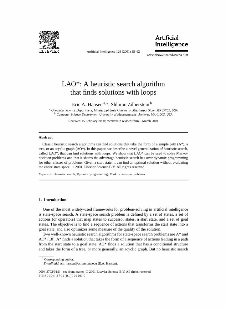
Table 3Trial-based RTDP

1. Start with an admissible evaluation function f .

2. Repeat the following trial n times.

Trial: Set the current state i to the start state and repeat the following steps m times or until a goal stateis reached.

(a) Improve the evaluation function by performing the following backup for the current state i,


[ci (a)+


].

(b) Take the action determined to be best for state i by the backup and change the current state i to thestate that results from a stochastic transition caused by the action.

3. Extract a partial policy from evaluation function f as follows. For each state i ∈ S that can be reachedfrom the start state by selecting actions greedily,


[ci (a)+


].

defined as maxi∈S |f U(i) − f L(i)|, gives a bound on the error of the current solution.A solution is ε-optimal if the error bound is less than ε. For any real number ε > 0, bothpolicy iteration and value iteration converge to an ε-optimal solution after a finite numberof iterations.

Real-time dynamic programming We are particularly interested in stochastic shortest-path problems that include a start state, s ∈ S, and for which the objective is to find asolution that minimizes the expected cost of reaching a goal state from the start state.Bertsekas [2] does not discuss this special case of a stochastic shortest-path problem.However, Barto et al. [1] do and note that it generalizes the classic AI search problemof finding a minimum-cost path from a start state to a goal state. Because findinga minimum-cost solution from a start state to a goal state is a special case of theproblem of finding a minimum-cost solution from every state to a goal state, it canbe solved using either policy iteration or value iteration. However, neither of thesealgorithms uses knowledge of the start state to focus computation on just those statesthat are reachable from the start state by following an optimal policy. Instead, both repeatan improvement step (the dynamic programming update) that updates the evaluationfunction for all states. In effect, both algorithms solve an MDP for all possible startingstates.

Barto et al. [1] describe an algorithm called real-time dynamic programming (RTDP)that avoids exhaustive evaluation of the state set. Table 3 summarizes trial-based RTDP,which solves an MDP by organizing computation as a sequence of trials. Each trial consistsof a sequence of steps. In each step, an action is selected based on lookahead search of


depth one or more, and the current state is updated based on the outcome of the action. Inaddition, the evaluation function is updated for a subset of states that includes the currentstate. At the beginning of each trial, the current state is set to the start state. A trial endswhen the goal state is reached, or after a specified number of steps. An important feature oftrial-based RTDP is that the evaluation function is only updated for states that are reachedfrom the start state when actions are selected greedily based on the current evaluationfunction. Thus, RTDP may ignore large regions of the state space. Barto et al. [1] provethat under certain reasonable conditions, RTDP converges (asymptotically) to an optimalsolution without necessarily evaluating the entire state space. They relate this result toheuristic search theory by showing that it generalizes the convergence theorem of Korf’slearning real-time heuristic search algorithm (LRTA*) [11].

Dean et al. [5] describe a related algorithm that performs policy iteration on a subsetof the states of an MDP, using various methods to identify the most relevant statesand gradually increasing the subset until eventual convergence (or until the algorithm isstopped). The subset of states is called an envelope and a policy defined on this subsetof states is called a partial policy. Adding states to an envelope is similar to expanding apartial solution in a search graph and the idea of using a heuristic to evaluate the fringestates of an envelope has been explored [6,21]. However, this algorithm is presented asa modification of policy iteration (and value iteration), rather than a generalization ofheuristic search. In particular, the assumption is explicitly made that convergence to anoptimal policy requires evaluating the entire state space.

Both RTDP and the related envelope algorithm are motivated by the problem of search(or planning) in real time. Both allow search to be interleaved with execution. The timeconstraint on search is usually the time before the next action needs to be executed, andboth Dean et al. [5] and Tash and Russell [21] describe decision-theoretic approaches tooptimizing the value of search in the interval between actions. The possibility of usingreal-time search to solve MDPs raises the following question: is there an off-line heuristicsearch algorithm that can solve MDPs? Before addressing this question directly, we reviewthe framework of state-space heuristic search.

2.2. Heuristic search in AND/OR graphs

Like an MDP, a state-space search problem is defined by a set of states (including a startstate and a set of goal states), a set of actions that cause state transitions, and a cost functionthat specifies costs for state transitions. The objective is to find a minimal-cost path fromthe start state to a goal state. It is customary to formalize a state-space search problem as agraph in which each node of the graph represents a problem state and each arc represents astate transition that results from taking an action. We use the same notation for state-spacesearch problems as for MDPs. Let S denote the set of possible states, let s ∈ S denote astart state that corresponds to the root of the graph, and let T ⊂ S denote a set of goal (orterminal) states that occur at the leaves of the graph. Let A denote a finite set of actionsand let A(i) denote the set of actions applicable in state i .

The most general state-space search problem considered in the AI literature is AND/ORgraph search. Following Martelli and Montanari [14] and Nilsson [18], we define anAND/OR graph as a hypergraph. Instead of arcs that connect pairs of states as in an


Fig. 1. (a) shows an OR node with two arcs leaving it, one for action a1 and one for action a2. Each arc leads to anAND node with two successor OR nodes, one for each possible successor state. (By convention, a square denotesan OR node and a circle denotes an AND node. In the terminology of decision analysis, a square correspondsto a choice node and a circle corresponds to a chance node.) (b) shows a state, indicated by a circle, with two2-connectors leaving it, one for action a1 and one for action a2. Each 2-connector leads to two possible successorstates. The representation on the right, using state nodes and k-connectors, is equivalent to the representation onthe left, which uses OR and AND nodes.

ordinary graph, a hypergraph has hyperarcs or k-connectors that connect a state to a setof k successor states. Fig. 1 relates the concept of OR and AND nodes to the concept of ahyperarc or k-connector.

A k-connector can be interpreted in different ways. In problem-reduction search, it isinterpreted as the transformation of a problem into k subproblems. We consider problemsof planning under uncertainty in which it is interpreted as an action with an uncertainoutcome. The action transforms a state into one of k possible successor states, with aprobability attached to each successor. We let pij (a) denote the probability that takingaction a in state i results in a transition to state j . This interpretation of AND/OR graphsis made by Martelli and Montanari [14] and Pattipati and Alexandridis [19], among others.

In AND/OR graph search, a solution takes the form of an acyclic subgraph called asolution graph, which is defined as follows:

• the start state belongs to a solution graph;• for every nongoal state in a solution graph, exactly one outgoing k-connector

(corresponding to an action) is part of the solution graph and each of its successorstates also belongs to the solution graph;

• every directed path in the solution graph terminates at a goal state.A cost function assigns a cost to each k-connector. Let ci(a) denote the cost for the k-connector that corresponds to taking action a in state i . We assume each goal state has acost of zero. A minimal-cost solution graph is found by solving the following system ofequations,

f ∗(i)={

0 if i is a goal state,mina∈A(i)

[ci(a)+ ∑

j∈S pij (a)f ∗(j)]

otherwise, (9)

where f ∗(i) denotes the cost of an optimal solution for state i and f ∗ is called the optimalevaluation function. Note that this is identical to the optimality equation defined for MDPsin Eq. (2), although we now assume the solution can be represented as an acyclic graph.This assumption means that a goal state can be reached from the start state after a boundednumber of actions (where the bound is equal to the longest path from the start state to agoal state). By contrast, a stochastic shortest-path problem has an unbounded or indefinite


horizon. Thus the traditional framework of AND/OR graph search does not directly applyto stochastic shortest-path problems.

AO* For state-space search problems that are formalized as AND/OR graphs, an optimalsolution graph can be found using the heuristic search algorithm AO*. Nilsson [16,17] firstdescribed a version of AO* for searching AND/OR trees to find a solution in the form ofa tree. Martelli and Montanari [13,14] generalized this algorithm for searching AND/ORgraphs to find a solution in the form of an acyclic graph. Nilsson [18] also used the nameAO* for this more general algorithm. Because any acyclic graph can be unfolded into anequivalent tree, the tree-search and graph-search versions of AO* solve the same class ofproblems. The graph-search version is more efficient when the same state can be reachedalong different paths because it avoids performing duplicate searches.

Like other heuristic search algorithms, AO* can find an optimal solution withoutconsidering every problem state. Therefore, a graph is not usually supplied explicitly tothe search algorithm. An implicit graph, G, is specified implicitly by a start state s anda successor function. The search algorithm constructs an explicit graph, G′, that initiallyconsists only of the start state. A tip or leaf state of the explicit graph is said to be terminalif it is a goal state; otherwise, it is said to be nonterminal. A nonterminal tip state can beexpanded by adding to the explicit graph its outgoing k-connectors (one for each action)and any successor states not already in the explicit graph.

AO* solves a state-space search problem by gradually building a solution graph,beginning from the start state. A partial solution graph is defined similarly to a solutiongraph, with the difference that the tip states of a partial solution graph may be nonterminalstates of the implicit AND/OR graph. A partial solution graph is defined as follows:

• the start state belongs to a partial solution graph;• for every nontip state in a partial solution graph, exactly one outgoing k-connector

(corresponding to an action) is part of the partial solution graph and each of itssuccessor states also belongs to the partial solution graph;

• every directed path in a partial solution graph terminates at a tip state of the explicitgraph.

As with solution graphs, there are many possible partial solution graphs and anevaluation function can be used to rank them. The cost of a partial solution graph is definedsimilarly to the cost of a solution graph. The difference is that if a tip state of a partialsolution graph is nonterminal, it does not have a cost that can be propagated backwards.Instead, we assume there is an admissible heuristic estimate h(i) of the minimal-costsolution graph for state i . A heuristic evaluation function h is said to be admissible ifh(i)� f ∗(i) for every state i . We can recursively calculate an admissible heuristic estimatef (i) of the optimal cost of any state i in the explicit graph as follows:

f (i)=

0 if i is a goal state,

h(i) if i is a nonterminal tip state,

mina∈A(i)[ci(a)+ ∑

j∈S pij (a)f (j)]

otherwise. (10)

The best partial solution graph can be determined at any time by propagating heuristicestimates from the tip states of the explicit graph to the start state. If we mark the action


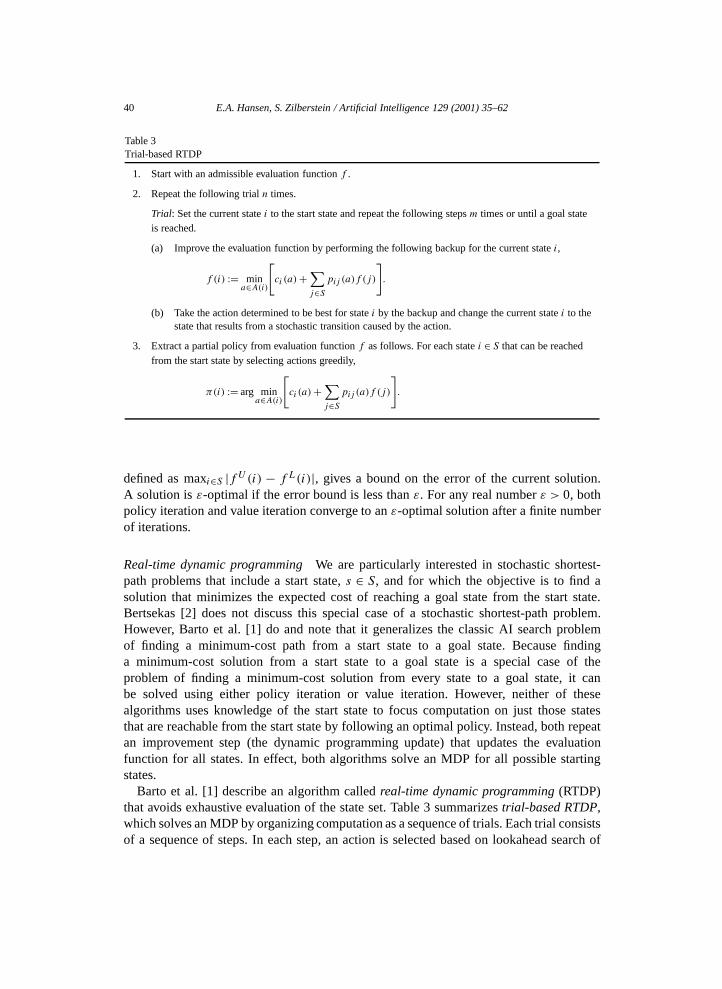
Table 4AO*

1. The explicit graph G′ initially consists of the start state s .

2. While the best solution graph has some nonterminal tip state:

(a) Expand best partial solution: Expand some nonterminal tip state n of the best partial solution graph andadd any new successor states to G′. For each new state i added to G′ by expanding n, if i is a goal statethen f (i) := 0; else f (i) := h(i).

(b) Update state costs and mark best actions:i. Create a set Z that contains the expanded state and all of its ancestors in the explicit graph along

marked action arcs. (I.e., only include ancestor states from which the expanded state can be reachedby following the current best solution.)

ii. Repeat the following steps until Z is empty.A. Remove from Z a state i such that no descendent of i in G′ occurs in Z.B. Set f (i) := mina∈A(i)[ci (a) + ∑

j pij (a)f (j)] and mark the best action for i. (Whendetermining the best action resolve ties arbitrarily, but give preference to the currently markedaction.)

3. Return an optimal solution graph.

that minimizes the value of each state, the best partial solution graph can be determined bystarting at the root of the graph and selecting the best action for each reachable state.

Table 4 outlines the algorithm AO* for finding a minimal-cost solution graph in anacyclic AND/OR graph. It interleaves forward expansion of the best partial solution witha cost revision step that updates estimated state costs and the best partial solution. In thesimplest version of AO*, the costs of the expanded state and all of its ancestor states in theexplicit graph are updated [13]. However, Martelli and Montanari [14] and Nilsson [18]note that the only ancestor states that may have their costs change are those from whichthe expanded state can be reached by taking marked actions (i.e., by choosing the bestaction for each state). Thus, the parenthetical remark in step 2(b)i of Table 4 indicates thata parent i of state j is not added to Z unless both the estimated cost of state j has changed,and state j can be reached from state i by choosing the best action for state i .

To simplify exposition, we have omitted from our outline of AO* a solve-labelingprocedure that is often included in the algorithm to improve efficiency. Briefly, a stateis labeled solved if it is a goal state or if all of its successor states are labeled solved.Labeling states as solved can improve the efficiency of the solution expansion step becauseit is unnecessary to search below a solved state for nonterminal tip states.

We also note that the best partial solution graph may have many nonterminal tip states.AO* works correctly no matter which of these tip states is chosen for expansion. However,the efficiency of AO* can be improved by using a good selection function to choose whichnonterminal tip state of the best partial solution graph to expand next. Possibilities includeselecting the tip state with the least estimated cost, or selecting the tip state with greatestprobability of being reached.

Although AND/OR graphs are usually assumed to be acyclic, the possibility of searchingcyclic AND/OR graphs has been studied [10]. In previous work, however, the solutiongraph is assumed to be acyclic. In Section 3, we consider how to generalize AND/ORgraph search to find cyclic solution graphs.


Dynamic programming and heuristic search It is possible to find an optimal solution toan AND/OR search problem using dynamic programming, instead of using AO*. Givena complete AND/OR graph containing every problem state, backwards induction can beperformed to find the optimal action for every state. Starting from goal states that havea cost of zero, the optimality equation can be solved by performing a backup for eachnonterminal state in backwards order from the leaves of the AND/OR graph toward theroot. Given the optimal cost for every successor of a state, the optimal cost for a state canbe determined by performing a single backup for that state. Because a backup is performedonce for each state and each backup has constant-time complexity, the complexity ofbackwards induction is linear in the number of states, even though the number of possiblesolution graphs is exponential in the number of states.

Dynamic programming is said to be an implicit-enumeration algorithm because it findsan optimal solution without evaluating all possible solutions. Once an optimal solutionfor a state is found, Bellman’s principle of optimality allows us to infer that an optimalsolution that reaches this state must include the solution that is optimal for this state. Thisis the reason for solving the problem in a backwards order from the leaves of the treeto the root, recursively combining solutions to increasingly larger subproblems until theoriginal problem is solved. Using Bellman’s principle of optimality to avoid enumeratingall possible solutions is sometimes called pruning by dominance.

Pruning by dominance, upon which dynamic programming relies, is a technique forpruning the space of solutions so that not every solution has to be evaluated in order to findthe best one. It is not a technique for pruning the state space. However, it is also possibleto prune states, and thus avoid generating the entire AND/OR graph, by using a techniquecalled pruning by bounds. This approach is taken by branch-and-bound algorithms. Toavoid evaluating the entire AND/OR graph, a branch-and-bound algorithm generates thegraph incrementally in a forward direction, beginning from the start state at the root of thegraph. It does not generate and evaluate subgraphs that can be pruned by comparing upperand lower bounds on their optimal cost. Given a lower-bound function (or equivalently, anadmissible heuristic evaluation function), it uses the following rule to avoid generating andevaluating a subgraph of an AND/OR graph: if a lower bound on the optimal cost of onek-connector (corresponding to one possible action) is greater than an upper bound on thecost of the state (determined by evaluating a subgraph that begins at another k-connector),then the first k-connector cannot be part of an optimal solution and the subgraph below itdoes not need to be evaluated.

Like branch-and-bound, best-first heuristic search can find an optimal solution withoutevaluating every state in the AND/OR graph. It is called “best-first” because it uses thelower-bound function to determine which tip state of the explicit graph to expand next, aswell as to prune the search space. Instead of expanding states in a depth-first (or breadth-first) order, the idea of best-first search is to expand states in an order that maximizes theeffect of pruning. The objective is to find an optimal solution while evaluating as little ofthe AND/OR graph as possible. A “best-first” order for expanding an AND/OR graph is toexpand the state that is most likely to be part of an optimal solution. This means expandinga tip state of the best partial solution graph.

So, in order to expand the graph in best-first order, AO* must identify the best partialsolution graph in an explicit graph. To do so, AO* uses backwards induction to propagate


state costs from the leaves of the explicit graph to its root. In other words, AO* usesdynamic programming in its cost revision step. In its forward expansion step, it uses thestart state and an admissible heuristic to focus computation on the part of the AND/ORgraph where an optimal solution is likely to be. In summary, AO* uses branch-and-bound inits forward expansion step and dynamic programming in its cost revision step. Integratingthese two techniques makes it possible to find an optimal solution as efficiently as possible,without evaluating the entire state space. It also suggests a similar strategy for solvingMDPs using heuristic search.

3. LAO*

We now describe LAO*, a simple generalization of AO* that can find solutions withloops. (The “L” in the name LAO* stands for “loop”.) LAO* is a heuristic search algorithmthat can find optimal solutions for MDPs without evaluating the entire state space. Thus, itprovides a useful alternative to dynamic programming algorithms for MDPs such as valueiteration and policy iteration.

It is straightforward to represent an indefinite-horizon MDP as an AND/OR graph. Welet each state of the AND/OR graph correspond to a state of the MDP and we let eachk-connector correspond to an action with k possible outcomes. In reviewing MDPs andAND/OR graph search, we used the same notation for their transition functions, costfunctions, and optimality equations, to help clarify the close relationship between thesetwo frameworks. A difference is that a solution to an indefinite-horizon MDP containsloops (i.e., it allows the same state to be visited more than once). Loops express indefinite-horizon behavior.

The classic AO* algorithm can only solve problems that have acyclic solutions becausethe backwards induction algorithm used in its cost revision step assumes an acyclicsolution. The key step in generalizing AO* to create LAO* is to recognize that the costrevision step of AO* is a dynamic programming algorithm, and to generalize this stepappropriately. Instead of using backwards induction, state costs can be updated by usinga dynamic programming algorithm for indefinite-horizon MDPs, such as policy iterationor value iteration. This simple generalization creates the algorithm LAO* summarized inTable 5.

As in AO*, the cost revision step of LAO* is only performed on the set of states thatincludes the expanded state and the states in the explicit graph from which the expandedstate can be reached by taking marked actions (i.e., by choosing the best action for eachstate). This is the set Z in step 2(b) of Table 5. The estimated cost of states that are not inthis subset are unaffected by any change in the cost of the expanded state or its ancestors.

The cost revision step of LAO* can be performed using either policy iteration or valueiteration. An advantage of using policy iteration is that it can compute an exact cost foreach state of the explicit graph after a finite number of iterations, based on the heuristicestimates at the tip states. When value iteration is used, convergence to exact state costsis asymptotic. However, this disadvantage is usually offset by the improved efficiency ofvalue iteration for larger problems.


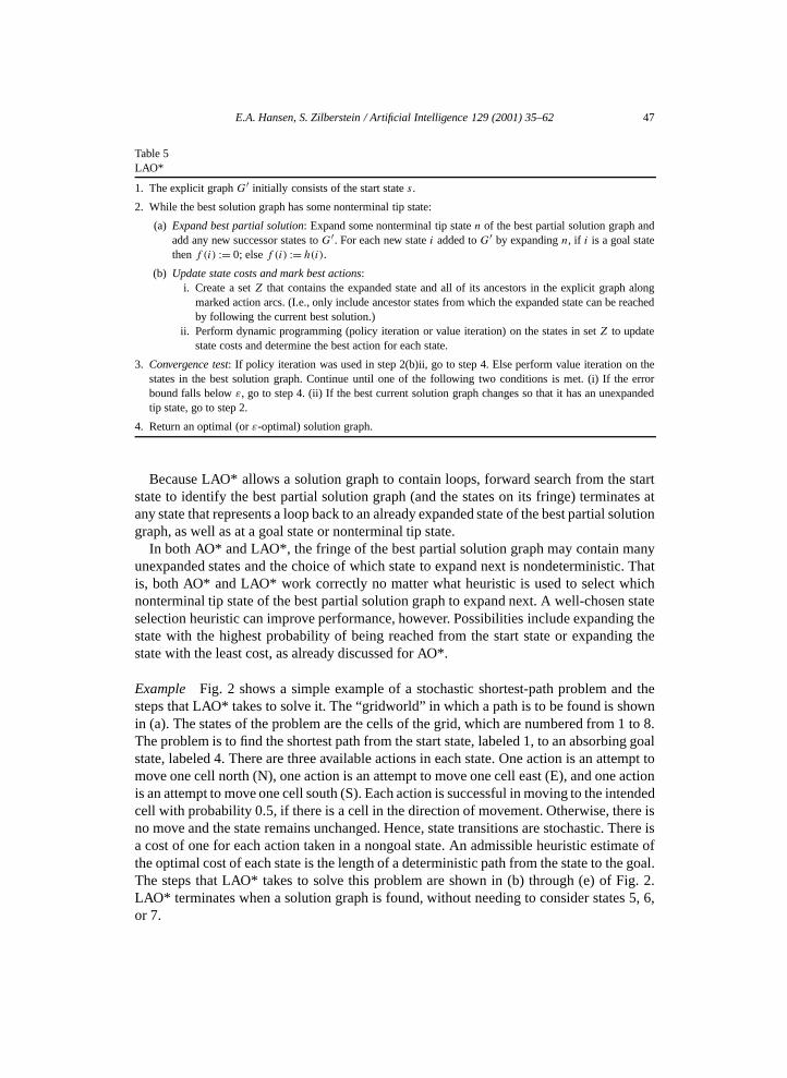
Table 5LAO*


2. While the best solution graph has some nonterminal tip state:

(a) Expand best partial solution: Expand some nonterminal tip state n of the best partial solution graph andadd any new successor states to G′. For each new state i added to G′ by expanding n, if i is a goal statethen f (i) := 0; else f (i) := h(i).

(b) Update state costs and mark best actions:i. Create a set Z that contains the expanded state and all of its ancestors in the explicit graph along

marked action arcs. (I.e., only include ancestor states from which the expanded state can be reachedby following the current best solution.)

ii. Perform dynamic programming (policy iteration or value iteration) on the states in set Z to updatestate costs and determine the best action for each state.

3. Convergence test: If policy iteration was used in step 2(b)ii, go to step 4. Else perform value iteration on thestates in the best solution graph. Continue until one of the following two conditions is met. (i) If the errorbound falls below ε, go to step 4. (ii) If the best current solution graph changes so that it has an unexpandedtip state, go to step 2.

4. Return an optimal (or ε-optimal) solution graph.

Because LAO* allows a solution graph to contain loops, forward search from the startstate to identify the best partial solution graph (and the states on its fringe) terminates atany state that represents a loop back to an already expanded state of the best partial solutiongraph, as well as at a goal state or nonterminal tip state.

In both AO* and LAO*, the fringe of the best partial solution graph may contain manyunexpanded states and the choice of which state to expand next is nondeterministic. Thatis, both AO* and LAO* work correctly no matter what heuristic is used to select whichnonterminal tip state of the best partial solution graph to expand next. A well-chosen stateselection heuristic can improve performance, however. Possibilities include expanding thestate with the highest probability of being reached from the start state or expanding thestate with the least cost, as already discussed for AO*.

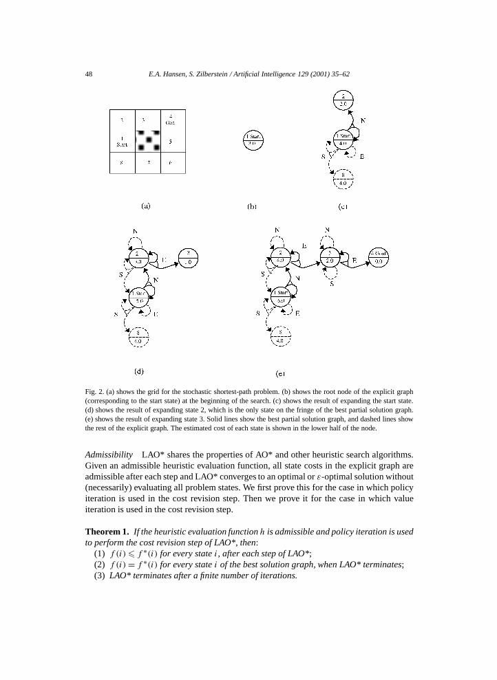
Example Fig. 2 shows a simple example of a stochastic shortest-path problem and thesteps that LAO* takes to solve it. The “gridworld” in which a path is to be found is shownin (a). The states of the problem are the cells of the grid, which are numbered from 1 to 8.The problem is to find the shortest path from the start state, labeled 1, to an absorbing goalstate, labeled 4. There are three available actions in each state. One action is an attempt tomove one cell north (N), one action is an attempt to move one cell east (E), and one actionis an attempt to move one cell south (S). Each action is successful in moving to the intendedcell with probability 0.5, if there is a cell in the direction of movement. Otherwise, there isno move and the state remains unchanged. Hence, state transitions are stochastic. There isa cost of one for each action taken in a nongoal state. An admissible heuristic estimate ofthe optimal cost of each state is the length of a deterministic path from the state to the goal.The steps that LAO* takes to solve this problem are shown in (b) through (e) of Fig. 2.LAO* terminates when a solution graph is found, without needing to consider states 5, 6,or 7.


Fig. 2. (a) shows the grid for the stochastic shortest-path problem. (b) shows the root node of the explicit graph(corresponding to the start state) at the beginning of the search. (c) shows the result of expanding the start state.(d) shows the result of expanding state 2, which is the only state on the fringe of the best partial solution graph.(e) shows the result of expanding state 3. Solid lines show the best partial solution graph, and dashed lines showthe rest of the explicit graph. The estimated cost of each state is shown in the lower half of the node.

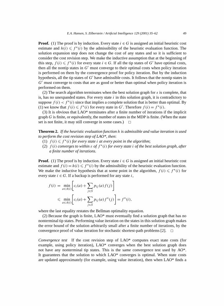
Admissibility LAO* shares the properties of AO* and other heuristic search algorithms.Given an admissible heuristic evaluation function, all state costs in the explicit graph areadmissible after each step and LAO* converges to an optimal or ε-optimal solution without(necessarily) evaluating all problem states. We first prove this for the case in which policyiteration is used in the cost revision step. Then we prove it for the case in which valueiteration is used in the cost revision step.

Theorem 1. If the heuristic evaluation function h is admissible and policy iteration is usedto perform the cost revision step of LAO*, then:

(1) f (i)� f ∗(i) for every state i , after each step of LAO*;(2) f (i)= f ∗(i) for every state i of the best solution graph, when LAO* terminates;(3) LAO* terminates after a finite number of iterations.


Proof. (1) The proof is by induction. Every state i ∈G is assigned an initial heuristic costestimate and h(i) � f ∗(i) by the admissibility of the heuristic evaluation function. Thesolution expansion step does not change the cost of any states and so it is sufficient toconsider the cost revision step. We make the inductive assumption that at the beginning ofthis step, f (i)� f ∗(i) for every state i ∈G. If all the tip states of G′ have optimal costs,then all the nontip states in G′ must converge to their optimal costs when policy iterationis performed on them by the convergence proof for policy iteration. But by the inductionhypothesis, all the tip states of G′ have admissible costs. It follows that the nontip states inG′ must converge to costs that are as good or better than optimal when policy iteration isperformed on them.

(2) The search algorithm terminates when the best solution graph for s is complete, thatis, has no unexpanded states. For every state i in this solution graph, it is contradictory tosuppose f (i) < f ∗(i) since that implies a complete solution that is better than optimal. By(1) we know that f (i)� f ∗(i) for every state in G′. Therefore f (i)= f ∗(i).

(3) It is obvious that LAO* terminates after a finite number of iterations if the implicitgraphG is finite, or equivalently, the number of states in the MDP is finite. (When the stateset is not finite, it may still converge in some cases.) ✷Theorem 2. If the heuristic evaluation function h is admissible and value iteration is usedto perform the cost revision step of LAO*, then:

(1) f (i)� f ∗(i) for every state i at every point in the algorithm;(2) f (i) converges to within ε of f ∗(i) for every state i of the best solution graph, after

a finite number of iterations.

Proof. (1) The proof is by induction. Every state i ∈G is assigned an initial heuristic costestimate and f (i)= h(i)� f ∗(i) by the admissibility of the heuristic evaluation function.We make the inductive hypothesis that at some point in the algorithm, f (i) � f ∗(i) forevery state i ∈G. If a backup is performed for any state i ,

f (i) = mina∈A(i)

[ci(a)+


]

� mina∈A(i)

[ci(a)+

∑j∈Spij (a)f

∗(j)]

= f ∗(i),

where the last equality restates the Bellman optimality equation.(2) Because the graph is finite, LAO* must eventually find a solution graph that has no

nonterminal tip states. Performing value iteration on the states in this solution graph makesthe error bound of the solution arbitrarily small after a finite number of iterations, by theconvergence proof of value iteration for stochastic shortest-path problems [2]. ✷Convergence test If the cost revision step of LAO* computes exact state costs (forexample, using policy iteration), LAO* converges when the best solution graph doesnot have any nonterminal tip states. This is the same convergence test used by AO*.It guarantees that the solution to which LAO* converges is optimal. When state costsare updated approximately (for example, using value iteration), then when LAO* finds a


solution graph that does not have any nonterminal tip states, this solution is not necessarilyoptimal. In this case, an additional convergence test can be used to determine when thesolution is ε-optimal.

The convergence test is simple and is summarized in step 3 of Table 5. It consists ofperforming value iteration on the set of states visited by the current best solution graph.Because value iteration may change the best action for some state, the best solution graphmay change from one iteration to the next. If the best solution graph changes to that itincludes a nonterminal tip state, control is passed from the convergence test back to themain algorithm so that the best partial solution can be expanded and re-evaluated. Whenthe best solution graph does not contain any nonterminal tip states, its error bound can becomputed. The convergence test is repeated until the error bound falls below ε. When itdoes, LAO* terminates with an ε-optimal solution.

The error bound is the difference between an upper and lower bound on the optimalcost of the start state of the solution. (This is different from the error bound for dynamicprogramming, which is the maximum difference over all states, not just the start state.)Because the current estimated cost of the start state is admissible, it serves as a lowerbound. An upper bound on the optimal cost of the start state is equal to f π (s)+ φπ (s)r ,where f π(s) is the estimated cost of the start state under the current policy π , φπ (s) isthe mean first passage time from the start state to any goal state under this policy, andr = maxi∈SG |f ′(i)− f (i)|, is the Bellman residual for this iteration of the convergencetest, where SG ⊆ S denotes the set of states visited by the current best solution graph.Because the estimated cost of every state in the explicit graph is admissible, the Bellmanresidual only needs to be computed for the states visited by the best solution in order todetermine the error bound of the solution. Similarly, first passage times only need to becomputed for states in the solution graph.

We note that while Barto et al. [1] prove that RTDP converges to an optimal solution,they do not describe a convergence test for RTDP or a method for computing an errorbound. The convergence test and error bound described here may also be adapted for useby RTDP.

Relationship to RTDP Both AO* and LAO*, as summarized in Tables 4 and 5, updatethe evaluation function for all ancestor states (along marked arcs) of an expanded state,whenever the best partial solution graph is expanded. They do so in order to maintainaccurate estimates of state costs for every state in the explicit graph. Updating theevaluation function for all states in the explicit graph can be time consuming, however,especially for LAO*, which uses a more complex dynamic programming algorithm.Therefore, it is useful to point out that LAO* only needs to update the evaluation functionfor the ancestor states of an expanded state that are in the best partial solution graph, inorder to ensure eventual convergence to an optimal or ε-optimal solution. To make thischange to LAO*, as summarized in Table 5, we simply change the phrase “explicit graph”to “best partial solution graph” in step 2(b)i of the algorithm. We described LAO* as weoriginally did to emphasize its similarity to AO*. (But if we made this same change toAO*, it would also still converge to an optimal solution.)

With this modification, the previous convergence theorems for LAO* still hold, by thefollowing reasoning. Consider any state i in the explicit graph that is not also in the best


partial solution graph. If f (i) is not updated, its value will be less than it would be if itwere updated—and therefore, it will still be admissible. Since f (i) is less than it would beif it were updated, it is more likely that it will be selected for inclusion in the best partialsolution graph. If it is not, it would not have been part of the best partial solution grapheven if it had been updated. If it is selected for inclusion in the best partial solution graph,then f (i) will be updated.

The observation that LAO* only needs to update f for states in the current best solutiongraph, in order to converge to an optimal solution, relates LAO* more closely to RTDP,which only updates f for states that can be reached from the start state by following thecurrent best solution.

4. Extensions

While RTDP is a real-time search algorithm and LAO* is an off-line search algorithm,both solve the same class of MDPs and both converge to an optimal solution withoutevaluating all problem states. An advantage of deriving LAO* from the heuristic searchalgorithm AO* is that it makes it easier to generalize refinements of classic heuristic searchalgorithms for use in solving MDPs more efficiently. To illustrate this, we describe someextensions of LAO* that are suggested by its derivation from AO* (and ultimately, fromA*). We conclude by briefly discussing the extension of LAO* to other MDPs besidesstochastic shortest-path problems.

4.1. Pathmax

In A* search, a heuristic evaluation function h is said to be consistent if it is bothadmissible and h(i) � ci(a) + h(j) for every state i ∈ S and action a ∈ A(i), where jis the successor state of state i when action a is taken. Consistency is a desirable propertybecause it ensures that state costs increase monotonically as the algorithm converges. If aheuristic evaluation function is admissible but not consistent, state costs need not increasemonotonically. However, they can be made to do so by adding a pathmax operation to theupdate step of the algorithm, as first suggested by Mérõ [15]. This common improvementof A* and AO* can also be made to LAO*.

For problems with stochastic state transitions, we generalize the definition of consistencyas follows: a heuristic evaluation function h is said to be consistent if it is both admissibleand h(i)� ci(a)+ ∑

j pij (a)h(j) for every state i ∈ S and action a ∈ A(i), where j is apossible successor state of state i when action a is taken. A pathmax operation is added toLAO* by changing the formula used to update state costs as follows:

f (i) := max

[f (i), min

a∈A(i)

[ci(a)+


]]. (10)

As it does for A* and AO*, use of the pathmax operation in LAO* can reduce the numberof states that are expanded to find an optimal solution, when the heuristic is not consistent.


4.2. Evaluation function decomposition

The A* search algorithm relies on a familiar f = g+ h decomposition of the evaluationfunction. Chakrabarti et al. [3] have shown that a similar decomposition of the evaluationfunction is possible for AO* and that it supports a weighted heuristic version of AO*. Wefirst show that this f = g+ h decomposition of the evaluation function can be extended toLAO*. Then we describe a similar weighted heuristic version of LAO*.

Each time a state i is generated by A*, a new estimate f (i) of the optimal cost from thestart state to a goal state is computed by adding g(i), the cost-to-arrive from the start stateto i , to h(i), the estimated cost-to-go from i to a goal state. Each time a state i is generatedby AO* or LAO*, the optimal cost from the start state to a goal state is also re-estimated.In this case, it is re-estimated by updating the estimated cost of every ancestor state of statei , including the start state. For the start state s, the estimated cost-to-go, denoted f (s), isdecomposed into g(s), the cost-to-arrive from the start state to a state on the fringe of thebest partial solution, and h(s), the estimated cost-to-go from the fringe of the best partialsolution to a goal state. In other words, g(s) represents the part of the solution cost that hasbeen explicitly computed so far and h(s) represents the part of the solution cost that is stillonly estimated. The same decomposition applies to every other state in the explicit graph.

For each state i , the values f (i), g(i), and h(i) are maintained, with f (i)= g(i)+h(i).After a state i is generated by AO* or LAO*, and before it is expanded, g(i) equals zeroand f (i) equals h(i). After state i is expanded, f (i) is updated in the same manner asbefore:


[ci(a)+


]. (11)

Having determined the action a that optimizes f (i), then g(i) and h(i) are updated asfollows:

g(i) := ci(a)+∑j∈Spij (a)g(j), (12)

h(i) :=∑j∈Spij (a)h(j). (13)

Once LAO* converges to a complete solution, note that h(i)= 0 and f (i)= g(i) for everystate i in the solution.

The possibility of decomposing the evaluation function of an MDP in this way elegantlyreflects the interpretation of an MDP as a state-space search problem that can be solved byheuristic search. It also makes it possible to create a weighted heuristic that can improvethe efficiency of LAO* in exchange for a bounded decrease in the optimality of the solutionit finds.

4.3. Weighted heuristic

Pohl [20] first described how to create a weighted heuristic and showed that it canimprove the efficiency of A* in exchange for a bounded decrease in solution quality. Given


the familiar decomposition of the evaluation function, f (i)= g(i)+h(i), a weightw, with0.5 � w � 1, is used to create a weighted heuristic, f (i)= (1 −w)g(i)+wh(i). Use ofthis heuristic guarantees that solutions found by A* are no more than a factor ofw/(1−w)worse than optimal [4]. Given a similar f = g+h decomposition of the evaluation functioncomputed by LAO*, it is straightforward to create a weighted version of LAO* that canfind an ε-optimal solution by evaluating a fraction of the states that LAO* might have toevaluate to find an optimal solution.

Note that a f = g+h decomposition of the evaluation function and a weighted heuristiccan also be used with RTDP. In fact, the idea of weighting a heuristic in order to finda bounded-optimal solution is explored by Ishida and Shimbo [9] for Korf’s LRTA*algorithm [11], which can be regarded as a special case of RTDP for solving deterministicsearch problems. They create a weighted heuristic by multiplying the initial heuristicestimate of each state’s value by a weight. (This approach is less flexible than one thatrelies on the f = g + h decomposition we have just described, however, because it doesnot allow the weight to be adjusted in the course of the search.) They find that a weightedheuristic can significantly reduce the number of states explored (expanded) by LRTA*without significantly decreasing the quality of the solution it finds.

4.4. Heuristic accuracy and search efficiency

In all heuristic search algorithms, three sets of states can be distinguished. The implicitgraph contains all problem states. The explicit graph contains those states that areevaluated in the course of the search. The solution graph contains those states that arereachable from the start state when the best solution is followed. The objective of a best-first heuristic search algorithm is to find an optimal solution graph while generating assmall an explicit graph as possible.

Like all heuristic search algorithms, the efficiency of LAO* depends crucially on theheuristic evaluation function that guides the search. The more accurate the heuristic, thefewer states need to be evaluated to find an optimal solution, that is, the smaller theexplicit graph generated by the search algorithm. For A*, the relationship between heuristicaccuracy and search efficiency has been made precise. Given two heuristic functions, h1

and h2, such that h1(i) � h2(i)� f ∗(i) for all states i , the set of states expanded by A*when guided by h2 is a subset of the set of states expanded by A* when guided by h1 [18].

A result this strong does not hold for AO*, or by extension, for LAO*. The reason it doesnot is that the selection of the next state to expand on the fringe of the best partial solutiongraph is nondeterministic. Although AO* and LAO* work correctly no matter which stateon the fringe of the best partial solution is expanded next, a particular choice may result insome states being expanded that would not be if the choice were different. Nevertheless,Chakrabarti et al. [3] show that a weaker result does hold for AO* and it is straightforwardto extend this result to LAO*.

Chakrabarti et al. [3] consider the worst-case set of states expanded by a searchalgorithm. Adapting their analysis, let W denote the worst-case set of states expandedby LAO*, defined as follows:

• the start state s is in W ;


• a state i is in W if there exists a partial solution graph p with an evaluation functionf p such that:– f p(s)� f ∗(s);– every nontip state of p is in W ;– i is a nonterminal tip state of p;

• no other states are inW .Given this definition, we have the following theorem.

Theorem 3. Given two heuristic functions, h1 and h2, such that h1(i)� h2(i)� f ∗(i) forall states i , the worst-case set of states expanded by LAO* when guided by h2 is a subsetof the worst-case set of states expanded by LAO* when guided by h1.

Proof. For any partial solution graph for start state s, we have

f1(s) = g(s)+ h1(s),

f2(s) = g(s)+ h2(s).

Since h1(s) � h2(s), we have f1(s) � f2(s). Thus, if f2(s) � f ∗(s), we also havef1(s)� f ∗(s). It follows that the worst-case set of states expanded by LAO* when guidedby h2 must be a subset of the worst-case set of states expanded by LAO* when guidedby h1. ✷

In other words, a more accurate heuristic does not necessarily make LAO* moreefficient. However, it makes it more efficient in the worst case. This result holds for a“pure” version of LAO* that updates state costs exactly in the dynamic-programming step.If LAO* updates state costs approximately, for example, by using value iteration with arelaxed criterion for convergence, the effect on the set of states expanded in the worst caseis not as clear.

4.5. Infinite-horizon problems

We have presented the results of this paper for stochastic shortest-path problems. ManyMDPs do not include terminal (or goal) states, or if they do, there is no guarantee that aterminal state can be reached from every other state. Problems that may never terminate arecalled infinite-horizon MDPs. For an infinite-horizon problem, one way to ensure that everystate has a finite expected cost is to discount future costs by a factor β , with 0 � β < 1. Forproblems for which discounting is not reasonable, other optimality criteria, such as averagecost per transition, can be adopted. Variations of policy and value iteration algorithms forthese other optimality criteria have been developed [2]. By incorporating them into LAO*,we claim that the results of this paper can be extended to infinite-horizon problems in astraightforward way. Hansen and Zilberstein [8] consider LAO* for discounted infinite-horizon MDPs and give convergence proofs.


5. Performance

We now examine the performance of LAO* on two test problems. The first is the racetrack problem used by Barto et al. [1] to illustrate the behavior of RTDP. The second is asimple example of a supply-chain management problem that has been studied extensivelyin operations research [12]. While further work is needed to fully evaluate LAO*, the twoproblems allow us to observe some important aspects of its behavior and to improve itsimplementation.

Race track problem To illustrate the behavior of RTDP, Barto et al. [1] describe a testproblem that involves a simple simulation of a race car on a track. The race track has anylength and shape, and includes a starting line at one end and a finish line at the other.The track is discretized into a grid of square cells, where each cell represents a possiblelocation of the car. Beginning at the starting line, the car attempts to move along the trackto the finish line. The state of the MDP is determined by the location of the car and its two-dimensional velocity. The car can change its velocity by ±1 in each dimension, for a totalof nine actions. The actual acceleration/deceleration that results from each action is zerowith some probability, in order to make state transitions stochastic. It is as if an attempt toaccelerate or decelerate sometimes fails because of an unpredictable slip on the track. Ifthe car hits the track boundary, it is moved back to the start state. For a full description ofthe problem, we refer to the paper by Barto et al. [1].

We test LAO* on an instance of this problem that has 21,371 states. When the race carit driven optimally, it avoids large parts of the track as well as dangerous velocities. Thus,only 2,248 states are visited by an optimal policy that starts at the beginning of the racetrack. Table 6 summarizes the performance of LAO* on this problem. It shows the numberof states evaluated by LAO* as a function of two different admissible heuristics. The “zeroheuristic” sets the initial heuristic cost of each state to zero. The “shortest-path heuristic”is computed by beginning from the set of goal states and determining the smallest possiblenumber of state transitions needed to reach a goal state, for each state. This more informed

Table 6Results for race track problem with 21,371 states. Optimal solution visits only 2,248states (Policy iteration is much slower than value iteration because exact policyevaluation has cubic complexity in the number of states, compared to the quadraticcomplexity of value iteration.)

Solution States Time to

Algorithm quality evaluated converge

Policy iteration Optimal 21,371 > 10 minutes

Value iteration Optimal 21,371 15.7 sec

LAO* w/ zero heuristic Optimal 18,195 10.7 sec

LAO* w/ shortest-path heuristic Optimal 14,252 4.7 sec

LAO* w/ weight = 0.6 Optimal 8,951 3.1 sec

LAO* w/ weight = 0.67 +4% 4,508 1.8 sec


heuristic enables LAO* to find an optimal solution by expanding fewer states. Weightingthe shortest-path heuristic allows a solution to be found by evaluating even fewer states,although the solution is not necessarily optimal. These results illustrate the importance ofheuristic accuracy in limiting the number of states evaluated by LAO*.

The number of states evaluated by LAO* is only one factor that influences its efficiency.Our experiments quickly revealed that a naive implementation of LAO* can be veryinefficient, even if it evaluates a fraction of the state space. The reason for this is that therunning time of LAO* is proportional to the total number of states evaluated multiplied bythe average number of times these states are evaluated. In a naive implementation of LAO*,the fact that fewer states are evaluated can be offset by an increase in the average numberof evaluations of these states. Using the race track problem as an example, expanding justone state on the fringe of the best partial solution graph at a time, and performing severaliterations of value iteration between each state expansion, results in many states beingevaluated tens of thousands of times before convergence.

We found that the performance of LAO* can be improved by using various techniquesto limit the number of times that states are evaluated. One technique is to expand multiplestates on the fringe of the best partial solution graph before performing the cost revisionstep. (Nilsson [18] makes a similar suggestion for AO*.) For this problem, expandingall states on the solution fringe before performing the cost revision step worked betterthan expanding any subset of the fringe states (although we do not claim that this is thebest strategy in general.) We also found it helpful to limit the number of iterations ofvalue iteration in each cost revision step, and to limit the number of ancestor states onwhich value iteration is performed. Because value and policy iteration are much morecomputationally expensive than expanding the best partial solution graph, finding ways tominimize the expense of the cost revision step usually improves the performance of LAO*.

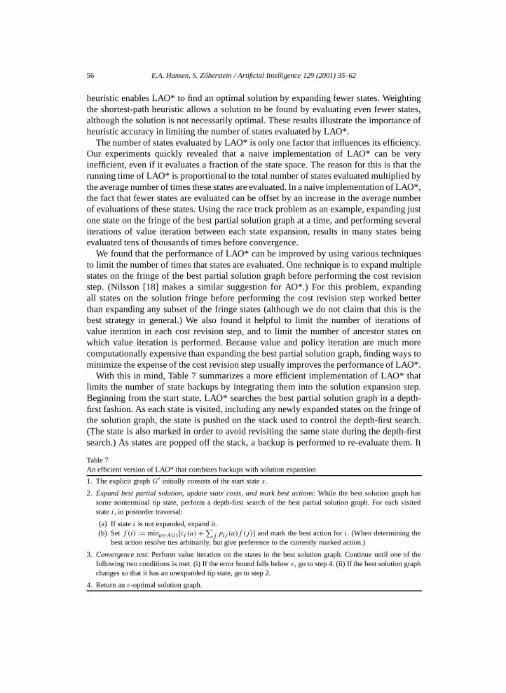
With this in mind, Table 7 summarizes a more efficient implementation of LAO* thatlimits the number of state backups by integrating them into the solution expansion step.Beginning from the start state, LAO* searches the best partial solution graph in a depth-first fashion. As each state is visited, including any newly expanded states on the fringe ofthe solution graph, the state is pushed on the stack used to control the depth-first search.(The state is also marked in order to avoid revisiting the same state during the depth-firstsearch.) As states are popped off the stack, a backup is performed to re-evaluate them. It

Table 7An efficient version of LAO* that combines backups with solution expansion


2. Expand best partial solution, update state costs, and mark best actions: While the best solution graph hassome nonterminal tip state, perform a depth-first search of the best partial solution graph. For each visitedstate i, in postorder traversal:

(a) If state i is not expanded, expand it.(b) Set f (i) := mina∈A(i)[ci (a)+

∑j pij (a)f (j)] and mark the best action for i. (When determining the

best action resolve ties arbitrarily, but give preference to the currently marked action.)

3. Convergence test: Perform value iteration on the states in the best solution graph. Continue until one of thefollowing two conditions is met. (i) If the error bound falls below ε, go to step 4. (ii) If the best solution graphchanges so that it has an unexpanded tip state, go to step 2.

4. Return an ε-optimal solution graph.


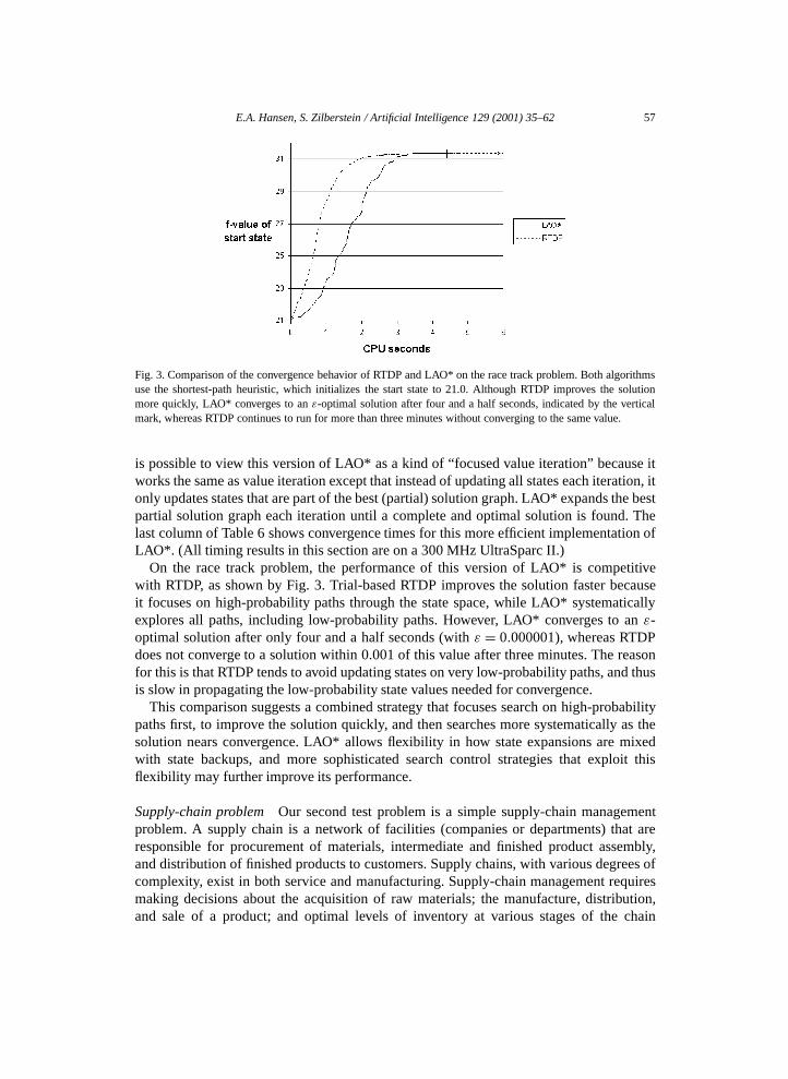
Fig. 3. Comparison of the convergence behavior of RTDP and LAO* on the race track problem. Both algorithmsuse the shortest-path heuristic, which initializes the start state to 21.0. Although RTDP improves the solutionmore quickly, LAO* converges to an ε-optimal solution after four and a half seconds, indicated by the verticalmark, whereas RTDP continues to run for more than three minutes without converging to the same value.

is possible to view this version of LAO* as a kind of “focused value iteration” because itworks the same as value iteration except that instead of updating all states each iteration, itonly updates states that are part of the best (partial) solution graph. LAO* expands the bestpartial solution graph each iteration until a complete and optimal solution is found. Thelast column of Table 6 shows convergence times for this more efficient implementation ofLAO*. (All timing results in this section are on a 300 MHz UltraSparc II.)

On the race track problem, the performance of this version of LAO* is competitivewith RTDP, as shown by Fig. 3. Trial-based RTDP improves the solution faster becauseit focuses on high-probability paths through the state space, while LAO* systematicallyexplores all paths, including low-probability paths. However, LAO* converges to an ε-optimal solution after only four and a half seconds (with ε = 0.000001), whereas RTDPdoes not converge to a solution within 0.001 of this value after three minutes. The reasonfor this is that RTDP tends to avoid updating states on very low-probability paths, and thusis slow in propagating the low-probability state values needed for convergence.

This comparison suggests a combined strategy that focuses search on high-probabilitypaths first, to improve the solution quickly, and then searches more systematically as thesolution nears convergence. LAO* allows flexibility in how state expansions are mixedwith state backups, and more sophisticated search control strategies that exploit thisflexibility may further improve its performance.

Supply-chain problem Our second test problem is a simple supply-chain managementproblem. A supply chain is a network of facilities (companies or departments) that areresponsible for procurement of materials, intermediate and finished product assembly,and distribution of finished products to customers. Supply chains, with various degrees ofcomplexity, exist in both service and manufacturing. Supply-chain management requiresmaking decisions about the acquisition of raw materials; the manufacture, distribution,and sale of a product; and optimal levels of inventory at various stages of the chain


of production. Such problems require sequential decision making under uncertainty(especially uncertainty about customer demand), and typically have very large statespaces [12].

We consider a small example of such a problem. To manufacture a product, say a lamp,we are dependent on supply of a part, say a flexible neck. Manufacture of the lamp dependson other parts as well, such as a lamp shade, bulb, basement, and cable, but we consideronly supply of one part for this example. Demand for the product is stochastic. The problemis to determine how many units of the product to produce, what price to sell the product for,how many units of the part to order, and what inventory to keep on hand. A complicatingfactor is that the cost of parts goes down if they are ordered in advance. Each order has aguaranteed delivery time. The longer the period between ordering and delivery, the lowerthe cost. This reflects the fact that advance notice allows the part manufacturer to increaseits own efficiency. We first specify the parameters of the problem. Then we describe theperformance of LAO*.

The problem state is defined by a tuple of state variables,

(ordAmt,ordTime, invProd, invPart,demand,price),

where ordAmt is the quantity of the part on order for each of the next ordTime time periods,invProd is the current inventory of the product, invPart is the current inventory of the part,demand defines a demand curve that gives the current demand for the product as a functionof price, and price is the current price of the product. We assume that each of these statevariables has a finite number of possible values, beginning from a minimum value andincreasing by a fixed step size to a maximum possible value. The size of the state space isthe cardinality of the cross-product of the domains of the state variables.

An action consists of two decisions. The first is to (possibly) change the price of thefinal product. The second is to (possibly) place a new order for parts. Each time period,a maximal number of new products is produced based on the available parts and theproduction capacity. Therefore, control of production is performed indirectly by limitingthe order of new parts. Once parts are available, we assume that it is beneficial to transformthem as soon as possible into complete products. To relax this assumption, one could addto each action a third component that controls the production level.

To limit the number of possible actions (in a reasonable way), we allow the price ofthe product to be increased or decreased by only the fixed step size each time period. Thenumber of actions and states is limited by the way we represent future orders. The mostgeneral representation is an arbitrary vector of orders [ordAmt1, ordAmt2, ordAmt3, . . . ,ordAmtn], where ordAmti represents the number of parts on order for delivery after i timeperiods. Instead, we assume the same number of parts, ordAmt, is ordered for deliveryin each of the next ordTime time periods. We also assume that existing orders form acommitment that cannot be canceled or changed. An action can only increase ordAmt orordTime, or both, up to some maximum. If no more parts are ordered, ordTime decreasesby one each time period until it reaches zero. Then it is possible to order any number ofparts for any number of periods.

As for the state transition function, we assume that actions have deterministic effects,but that demand is stochastic. Demand for the product is given by the formula

demand(price)= demand · eα·price,


where α is a constant that characterizes this product, and demand is a state variable thatchanges stochastically each time period. With probability 0.3, it increases by one unit; withprobability 0.3, it decreases by one unit; and with probability 0.4, it remains unchanged.The transition probabilities change when the demand variable is at its maximum orminimum value. At its maximum value, it decreases with probability 0.4 and otherwiseremains unchanged. At its minimum value, it increases with probability 0.4 and otherwiseremains unchanged.

We treat this as a reward-maximization problem (which is a simple modification of acost-minimization problem). The overall reward is the difference between the income fromselling products and the associated costs. In each action cycle, the immediate income isthe number of products sold times the price of a product. The immediate cost has threecomponents: production cost, inventory storage cost, and the cost of ordering parts. Theformer two are linear functions defined by the unit production cost, CostProd, and the unitstorage costs for inventory, InvCostPart and InvCostProd. The cost of an order depends ona variable unit cost for a part, which is a monotonically decreasing function of time thepart is ordered in advance. The minimum cost, MinCostPart, applies if the part is orderedat least tmin time periods in advance. The maximum cost, MaxCostPart, applies if the partif ordered less than tmax time periods in advance. The cost changes linearly between tmax

and tmin.The objective is to maximize the discounted sum of rewards over an infinite horizon.

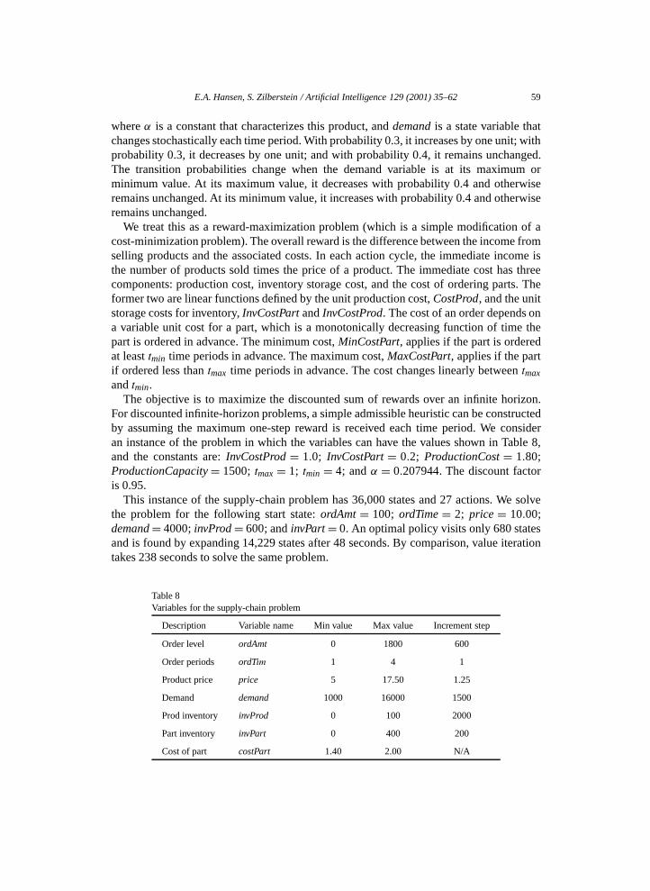
For discounted infinite-horizon problems, a simple admissible heuristic can be constructedby assuming the maximum one-step reward is received each time period. We consideran instance of the problem in which the variables can have the values shown in Table 8,and the constants are: InvCostProd = 1.0; InvCostPart = 0.2; ProductionCost = 1.80;ProductionCapacity = 1500; tmax = 1; tmin = 4; and α = 0.207944. The discount factoris 0.95.

This instance of the supply-chain problem has 36,000 states and 27 actions. We solvethe problem for the following start state: ordAmt = 100; ordTime = 2; price = 10.00;demand = 4000; invProd = 600; and invPart = 0. An optimal policy visits only 680 statesand is found by expanding 14,229 states after 48 seconds. By comparison, value iterationtakes 238 seconds to solve the same problem.

Table 8Variables for the supply-chain problem

Description Variable name Min value Max value Increment step

Order level ordAmt 0 1800 600

Order periods ordTim 1 4 1

Product price price 5 17.50 1.25

Demand demand 1000 16000 1500

Prod inventory invProd 0 100 2000

Part inventory invPart 0 400 200

Cost of part costPart 1.40 2.00 N/A


We have experimented with additional problem instances created by varying theparameters of this problem and found that LAO* consistently outperforms value iteration.It is well-suited for this supply-chain problem because, regardless of the starting state,an optimal policy is to try to enter a certain steady state of production and orders, and thissteady state involves a small fraction of the state space (less than 2% in the above example).While it is difficult to generalize these results to other problems, or even to more complexsupply-chain problems, they improve our intuition about the performance of LAO* andshow that it can be a useful algorithm.

For what types of problem is LAO* useful? Given a start state and an admissible heuristicto guide forward expansion of a partial solution, LAO* can find an optimal solution withoutevaluating the entire state space. However, it only enjoys this advantage for problems forwhich an optimal solution visits a fraction of the state space, beginning from the start state.Many problems have this property, including our two test problems. But many do not. Itwould be useful to have a way of identifying problems for which LAO* is effective. Theredoes not appear to be an easy answer to this question. Nevertheless, we make a few remarksin this direction.

One relevant factor appears to be how much overlap there is between the sets ofsuccessor states for different actions, taken in the same state. If there is little overlap,a policy can more easily constrain the set of reachable states. If there is much (or evencomplete) overlap, it cannot. For example, each action in the race track problem has twopossible successor states. The action of accelerating or decelerating either succeeds or fails.(It fails due to a slip on the track. This is the stochastic element of the problem.) Thus, theoverlap between the successor states for different actions is limited to the case of failure.Otherwise, each action has a distinct successor state. Now, consider the following slightmodification of the race track problem. With some small probability, each action has theeffect of any other action. In this case, every action has the same set of possible successorstates and the choice of one action instead of another does not affect the set of reachablestates. With this change to the race track problem, every policy visits all the states of therace track problem.

Even for problems for which an optimal policy visits all (or most) of the state space,LAO* may provide a useful framework for finding partial solutions under time constraints.Instead of finding a complete policy, it can focus computation on finding a policy for asubset of states that is most likely to be reached from the starting state. This approachto solving MDPs approximately has been explored by Dean et al. [5]. The framework ofLAO* relates this approach more closely to classic heuristic search algorithms.

6. Conclusion

We have presented a generalization of AO*, called LAO*, that can find solutions withloops, and we have shown that it can be used to solve indefinite-horizon MDPs. Like otherheuristic search algorithms, LAO* can find an optimal solution for a start state withoutevaluating the entire state space.


Although real-time search has been applied to MDPs before [1,5,6,21], LAO* is the firstoff-line heuristic search algorithm for MDPs. The derivation of LAO* from the classicheuristic search algorithm AO* provides a foundation for a heuristic search approach toMDPs. It also makes it easier to generalize enhancements of classic search algorithms foruse in solving MDPs more efficiently. The results presented in this paper illustrate therelevance of the rich body of AI research on heuristic search to the problem of solvingMDPs more efficiently. They also help to clarify the relationship between classic AI searchtechniques and dynamic programming algorithms developed in operations research.

Acknowledgements

We thank Dietrich Eisenhardt for implementing the supply chain example and runningthe experiments on it. We thank the anonymous reviewers for helpful comments. Supportfor this work was provided in part by the National Science Foundation under grant IIS-9984952 to the first author and grants IRI-9624992 and IRI-9634938 to the second author.

References

[1] A.G. Barto, S.J. Bradtke, S.P. Singh, Learning to act using real-time dynamic programming, ArtificialIntelligence 72 (1995) 81–138.

[2] D. Bertsekas, Dynamic Programming and Optimal Control, Athena Scientific, Belmont, MA, 1995.[3] P.P. Chakrabarti, S. Ghose, S.C. DeSarkar, Admissibility of AO* when heuristics overestimate, Artificial

Intelligence 34 (1988) 97–113.[4] H.W. Davis, A. Bramanti-Gregor, J. Wang, The advantages of using depth and breadth components in

heuristic search, in: Z.W. Ras, L. Saitta (Eds.), Methodologies for Intelligent Systems Vol. 3, North-Holland,Amsterdam, 1989, pp. 19–28.

[5] T. Dean, L.P. Kaelbling, J. Kirman, A. Nicholson, Planning under time constraints in stochastic domains,Artificial Intelligence 76 (1995) 35–74.

[6] R. Dearden, C. Boutilier, Integrating planning and execution in stochastic domains, in: Proc. TenthConference on Uncertainty in Artificial Intelligence, Washington, DC, 1994, pp. 162–169.

[7] R. Dechter, J. Pearl, Generalized best-first search strategies and the optimality of A*, J. ACM 32 (1985)505–536.

[8] E.A. Hansen, S. Zilberstein, Heuristic search in cyclic AND/OR graphs, in: Proc. AAAI-98, Madison, WI,1998, pp. 412–418.

[9] T. Ishida, M. Shimbo, Improving the learning efficiencies of realtime search, in: Proc. AAAI-96, Portland,OR, 1996, pp. 305–310.

[10] P. Jiménez, C. Torras, An efficient algorithm for searching implicit AND/OR graphs with cycles, ArtificialIntelligence 124 (2000) 1–30.

[11] R. Korf, Real-time heuristic search, Artificial Intelligence 42 (1990) 189–211.[12] Z. Lian, A. Deshmukh, J. Wang, Optimal frozen period in a periodic review inventory model with updateable

demand forecasts, in: Proc. 15th International Conference on Production Research, 1999.[13] A. Martelli, U. Montanari, Additive AND/OR graphs, in: Proc. IJCAI-73, Stanford, CA, 1973, pp. 1–11.[14] A. Martelli, U. Montanari, Optimizing decision trees through heuristically guided search, Comm.

ACM 21 (12) (1978) 1025–1039.[15] L. Mérõ, A heuristic search algorithm with modifiable estimate, Artificial Intelligence 23 (1) (1984) 13–27.[16] N.J. Nilsson, Search problem-solving and game-playing trees for minimal cost solutions, in: A. Morrell

(Ed.), Information Processing 68, Vol. 2, North-Holland, Amsterdam, 1969, pp. 1556–1562.[17] N.J. Nilsson, Problem Solving Methods in Artificial Intelligence, McGraw-Hill, New York, 1971.


[18] N.J. Nilsson, Principles of Artificial Intelligence, Tioga Publishing, Palo Alto, CA, 1980.[19] K.R. Pattipati, M.G. Alexandridis, Application of heuristic search and information theory to sequential fault

diagnosis, IEEE Trans. Systems Man Cybernet. 20 (4) (1990) 872–887.[20] I. Pohl, First results on the effect of error in heuristic search, Machine Intelligence 5 (1973) 219–236.[21] J. Tash, S.J. Russell, Control strategies for a stochastic planner, in: Proc. AAAI-94, Seattle, WA, 1994,

pp. 1079–1085.

Documents

LAO*: A heuristic search algorithm that ﬁnds solutions ...rbr.cs.umass.edu/papers/HZaij01b.pdfArtiﬁcial Intelligence 129 (2001) 35–62 LAO*: A heuristic search algorithm that

LAO: A heuristic search algorithm that ﬁnds solutions ...rbr.cs.umass.edu/papers/HZaij01b.pdfArtiﬁcial Intelligence 129 (2001) 35–62 LAO: A heuristic search algorithm that