Embed Size (px)
Citation preview
Laplace Transform
BIOE 4200
Why use Laplace Transforms?
Find solution to differential equation using algebra
Relationship to Fourier Transform allows easy way to characterize systems
No need for convolution of input and differential equation solution
Useful with multiple processes in system
How to use Laplace
Find differential equations that describe system
Obtain Laplace transformPerform algebra to solve for output or
variable of interestApply inverse transform to find solution
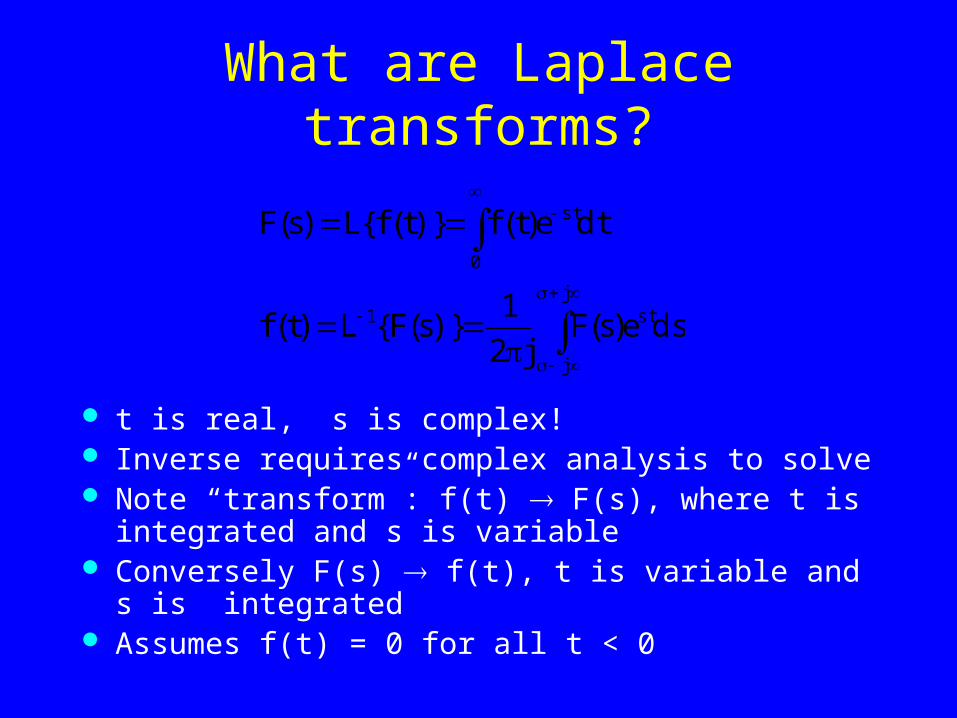
What are Laplace transforms?
j
j
st1
0
st
dse)s(Fj2
1)}s(F{L)t(f
dte)t(f)}t(f{L)s(F
t is real, s is complex! Inverse requires complex analysis to solve Note “transform”: f(t) F(s), where t is integrated and
s is variable Conversely F(s) f(t), t is variable and s is
integrated Assumes f(t) = 0 for all t < 0
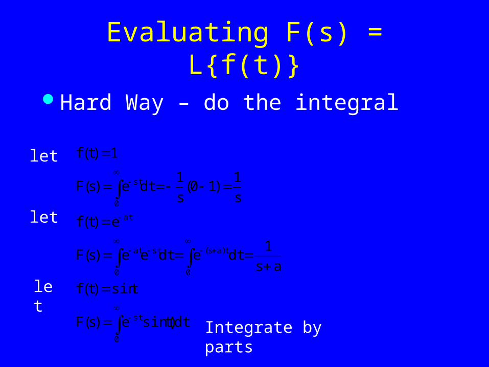
Evaluating F(s) = L{f(t)}
Hard Way – do the integral
0
st
0 0
t)as(stat
at
0
st
dt)tsin(e)s(F
tsin)t(f
as
1dtedtee)s(F
e)t(f
s
1)10(
s
1dte)s(F
1)t(flet
let
let
Integrate by parts
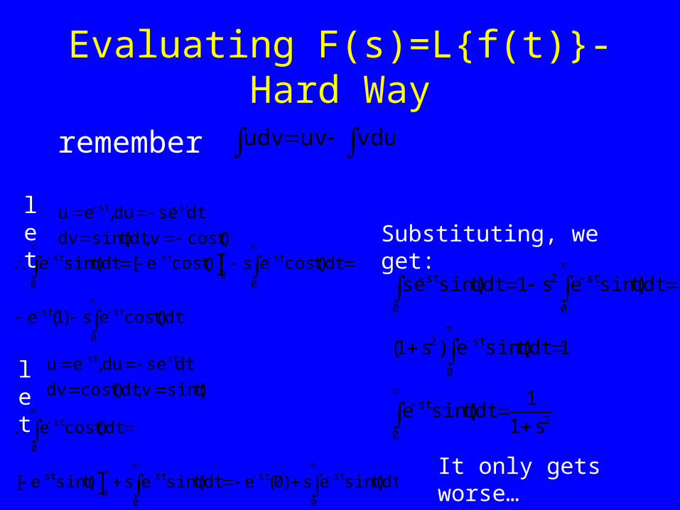
Evaluating F(s)=L{f(t)}- Hard Way
remember vduuvudv
)tcos(v,dt)tsin(dv
dtsedu,eu stst
0
stst
0 0
st
0
stst
dt)tcos(es)1(e
dt)tcos(es)tcos(e[dt)tsin(e ]
)tsin(v,dt)tcos(dv
dtsedu,eu stst
0
stst
0
st
0
st
0
st
dt)tsin(es)0(edt)tsin(es)tsin(e[
dt)tcos(e
]
20
st
0
st2
0 0
st2st
s1
1dt)tsin(e
1dt)tsin(e)s1(
dt)tsin(es1dt)tsin(se
let
let
Substituting, we get:
It only gets worse…
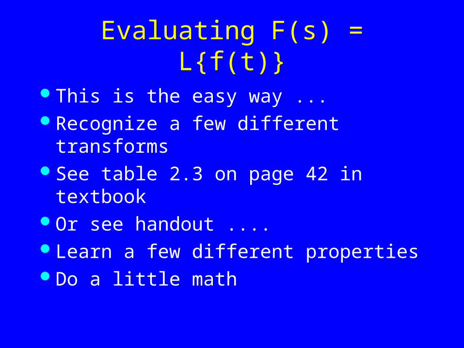
Evaluating F(s) = L{f(t)}
This is the easy way ...Recognize a few different transformsSee table 2.3 on page 42 in textbookOr see handout .... Learn a few different properties Do a little math
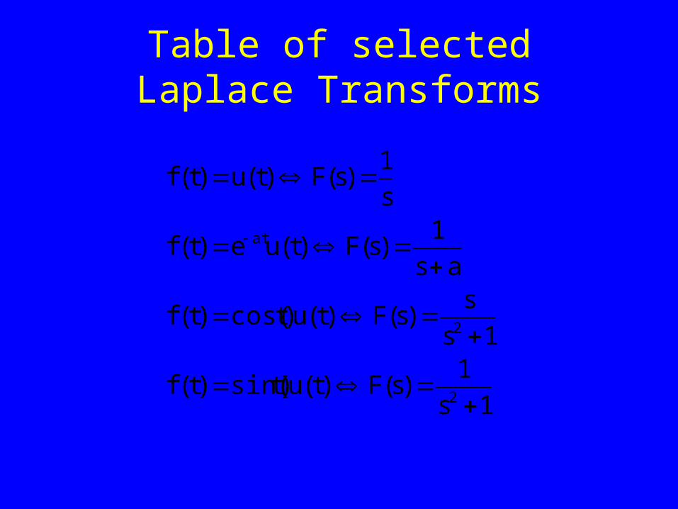
Table of selected Laplace Transforms
1s
1)s(F)t(u)tsin()t(f
1s
s)s(F)t(u)tcos()t(f
as
1)s(F)t(ue)t(f
s
1)s(F)t(u)t(f
2
2
at
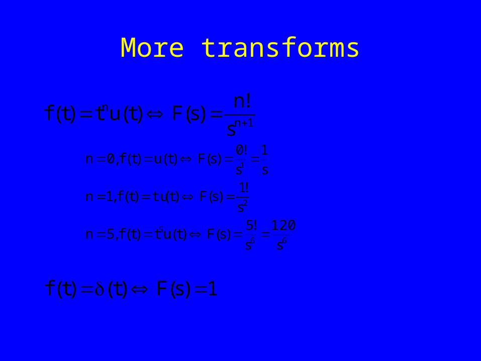
More transforms
1nn
s
!n)s(F)t(ut)t(f
665
2
1
s
120
s
!5)s(F)t(ut)t(f,5n
s
!1)s(F)t(tu)t(f,1n
s
1
s
!0)s(F)t(u)t(f,0n
1)s(F)t()t(f
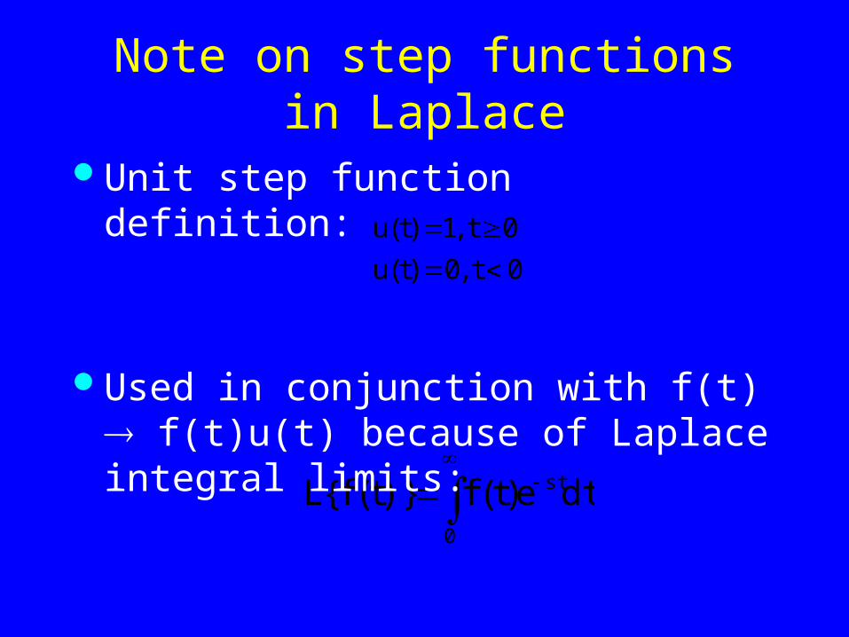
Note on step functions in Laplace
0
stdte)t(f)}t(f{L
0t,0)t(u
0t,1)t(u
Unit step function definition:
Used in conjunction with f(t) f(t)u(t) because of Laplace integral limits:
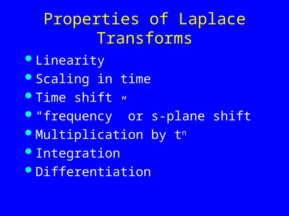
Properties of Laplace Transforms
LinearityScaling in timeTime shift“frequency” or s-plane shiftMultiplication by tn
IntegrationDifferentiation
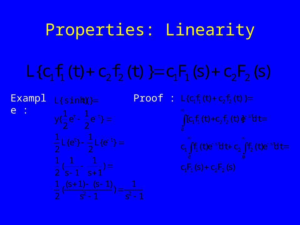
Properties: Linearity
)s(Fc)s(Fc)}t(fc)t(fc{L 22112211 Example :
1s
1)
1s
)1s()1s((
2
1
)1s
1
1s
1(
2
1
}e{L2
1}e{L
2
1
}e2
1e
2
1{y
)}t{sinh(L
22
tt
tt
Proof :
)s(Fc)s(Fc
dte)t(fcdte)t(fc
dte)]t(fc)t(fc[
)}t(fc)t(fc{L
2211
0
st22
0
st11
st22
0
11
2211
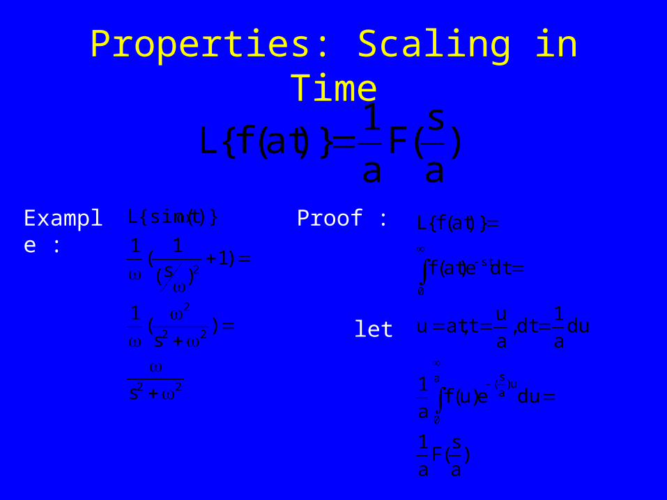
)a
s(F
a
1)}at(f{L
Example :
22
22
2
2
s
)s
(1
)1)s(
1(
1
)}t{sin(L
Proof :
)a
s(F
a
1
due)u(fa
1
dua
1dt,
a
ut,atu
dte)at(f
)}at(f{L
a
0
u)a
s(
0
st
let
Properties: Scaling in Time
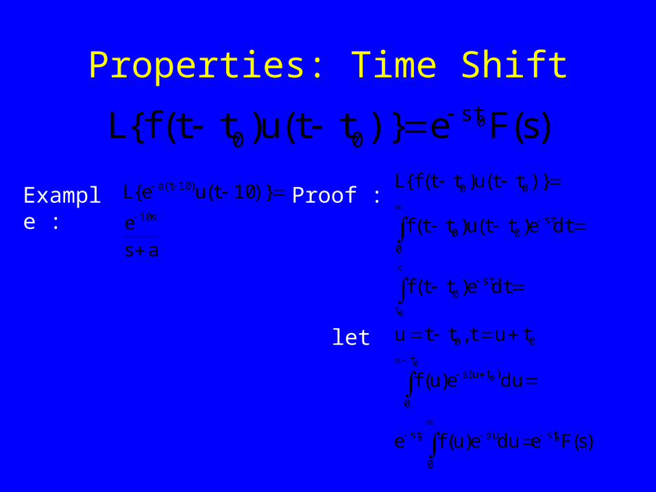
Properties: Time Shift
)s(Fe)}tt(u)tt(f{L 0st00
Example :
as
e
)}10t(ue{Ls10
)10t(a
Proof :
)s(Fedue)u(fe
due)u(f
tut,ttu
dte)tt(f
dte)tt(u)tt(f
)}tt(u)tt(f{L
00
0
0
0
st
0
sust
t
0
)tu(s
00
t
st0
0
st00
00
let
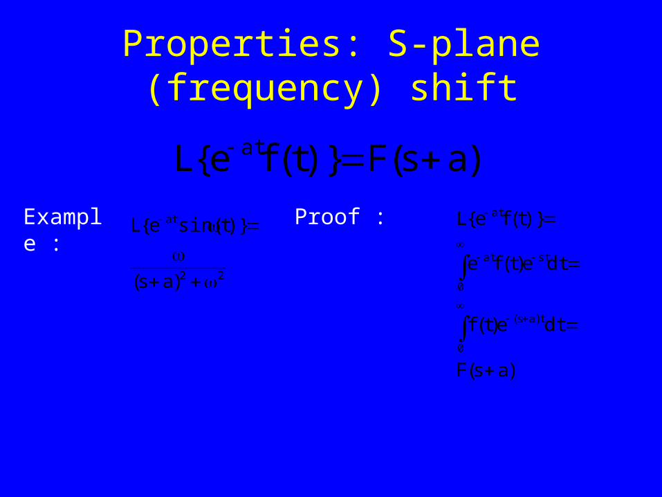
Properties: S-plane (frequency) shift
)as(F)}t(fe{L at
Example :
22
at
)as(
)}tsin(e{L
Proof :
)as(F
dte)t(f
dte)t(fe
)}t(fe{L
0
t)as(
0
stat
at
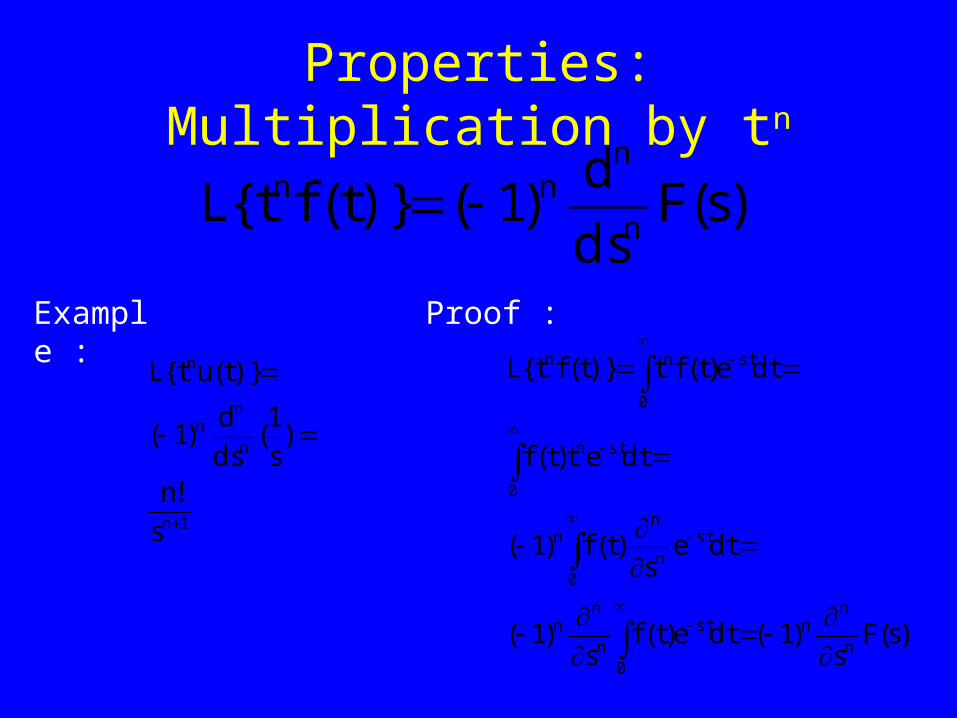
Properties: Multiplication by tn
)s(Fds
d)1()}t(ft{L
n
nnn
Example :
1n
n
nn
n
s
!n
)s
1(
ds
d)1(
)}t(ut{L
Proof :
)s(Fs
)1(dte)t(fs
)1(
dtes
)t(f)1(
dtet)t(f
dte)t(ft)}t(ft{L
n
nn
0
stn
nn
0
stn
nn
0
stn
0
stnn
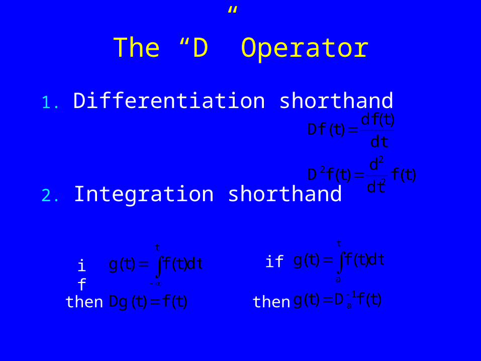
The “D” Operator
1. Differentiation shorthand
2. Integration shorthand)t(f
dt
d)t(fD
dt
)t(df)t(Df
2
22
)t(f)t(Dg
dt)t(f)t(gt
)t(fD)t(g
dt)t(f)t(g
1a
t
a
if
then then
if
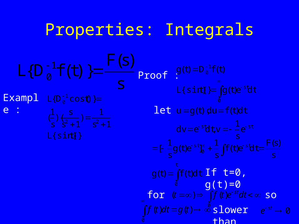
Properties: Integrals
s
)s(F)}t(fD{L 1
0
Example :
)}t{sin(L1s
1)
1s
s)(
s
1(
)}tcos(D{L
22
10
Proof :
let
stst
0
st
10
es
1v,dtedv
dt)t(fdu),t(gu
dte)t(g)}t{sin(L
)t(fD)t(g
t
0
st0
st
dt)t(f)t(g
s
)s(Fdte)t(f
s
1]e)t(g
s
1[
0
)()( dtetft st
If t=0, g(t)=0
for so
slower than
0
)()( tgdttf 0 ste
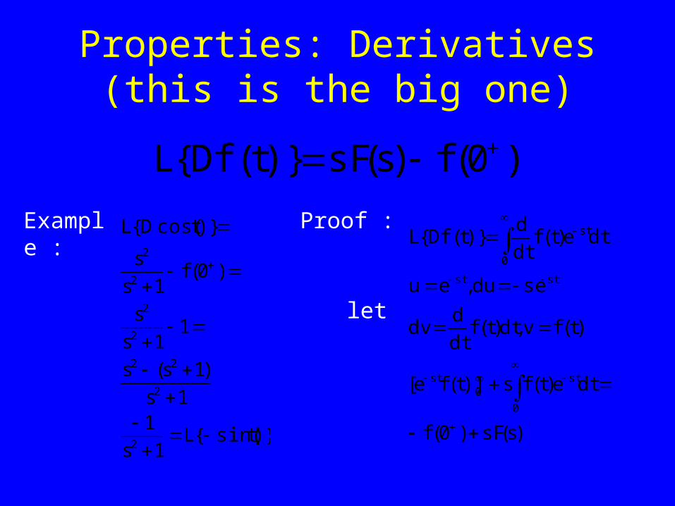
Properties: Derivatives(this is the big one)
)0(f)s(sF)}t(Df{L Example :
)}tsin({L1s
11s
)1s(s
11s
s
)0(f1s
s
)}tcos(D{L
2
2
22
2
2
2
2
Proof :
)s(sF)0(f
dte)t(fs)]t(fe[
)t(fv,dt)t(fdt
ddv
sedu,eu
dte)t(fdt
d)}t(Df{L
0
st0
st
stst
0
st
let
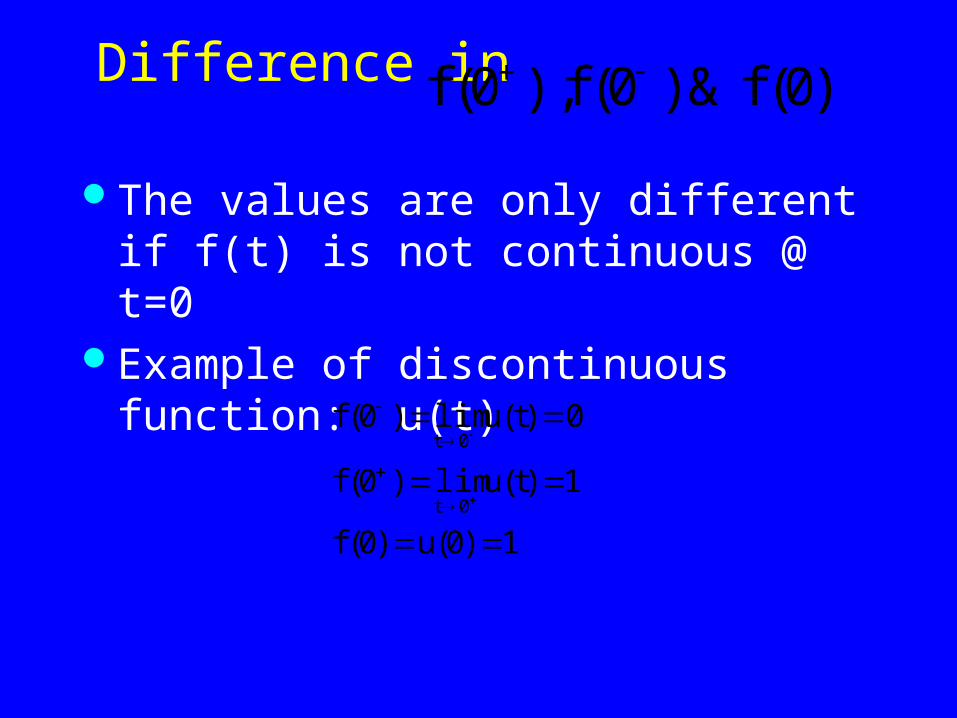
Difference in
The values are only different if f(t) is not continuous @ t=0
Example of discontinuous function: u(t)
)0(f&)0(f),0(f
1)0(u)0(f
1)t(ulim)0(f
0)t(ulim)0(f
0t
0t
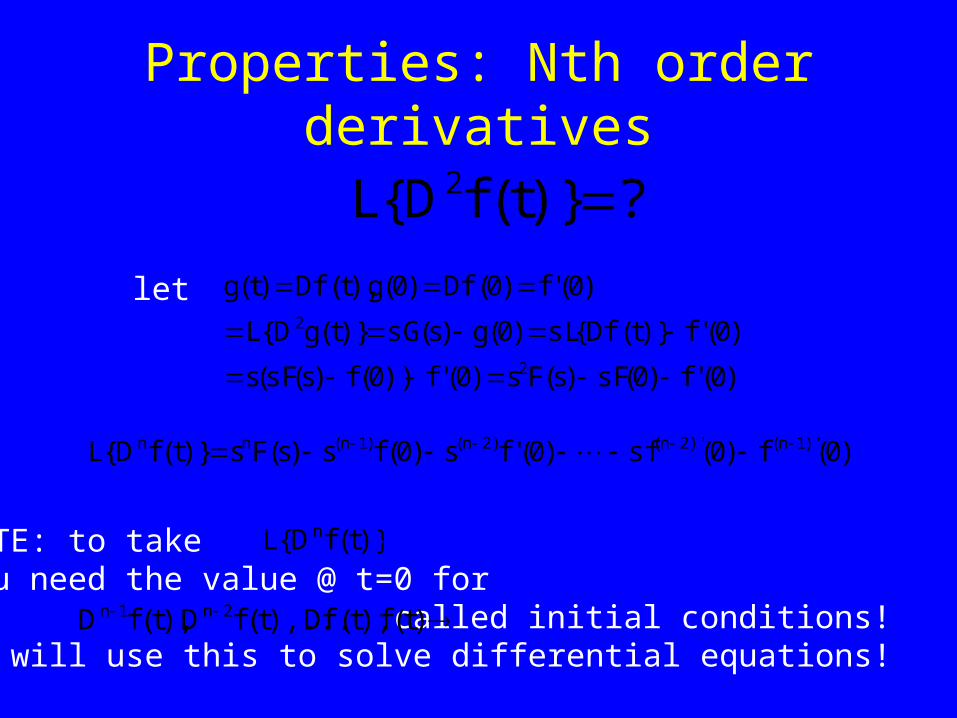
?)}t(fD{L 2
)0('f)0(sF)s(Fs)0('f))0(f)s(sF(s
)0('f)}t(Df{sL)0(g)s(sG)}t(gD{L
)0('f)0(Df)0(g),t(Df)t(g
2
2
let
)0(f)0(sf)0('fs)0(fs)s(Fs)}t(fD{L )'1n()'2n()2n()1n(nn
NOTE: to takeyou need the value @ t=0 for
called initial conditions!We will use this to solve differential equations!
)t(f),t(Df),...t(fD),t(fD 2n1n
)}t(fD{L n
Properties: Nth order derivatives
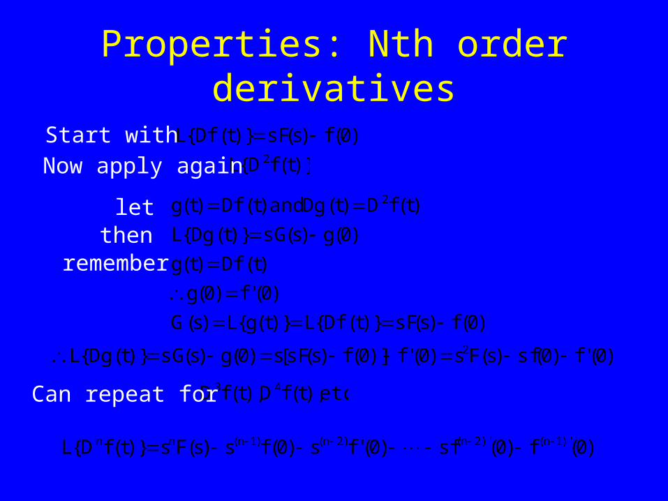
Properties: Nth order derivatives
)0(f)s(sF)}t(Df{L )}t(fD{L 2
)0(f)s(sF)}t(Df{L)}t(g{L)s(G
)0('f)0(g
)t(Df)t(g
)0(g)s(sG)}t(Dg{L
)t(fD)t(Dgand)t(Df)t(g 2
)0('f)0(sf)s(Fs)0('f)]0(f)s(sF[s)0(g)s(sG)}t(Dg{L 2
.etc),t(fD),t(fD 43
Start with
Now apply again
letthen
remember
Can repeat for
)0(f)0(sf)0('fs)0(fs)s(Fs)}t(fD{L )'1n()'2n()2n()1n(nn
Relevant Book Sections
Modeling - 2.2Linear Systems - 2.3, page 38 onlyLaplace - 2.4Transfer functions – 2.5 thru ex 2.4