1

Laplace's Equation in Cartesian Coordinates and Satellite Altimetry(Copyright 2002, David T. Sandwell)

Variations in the gravitational potential and the gravitational force are caused by localvariations in the mass distribution in the Earth. As described in an earlier lecture, we decomposethe gravity field of the Earth into three fields:

• the main field due to the total mass of the earth;• the second harmonic due to the flattening of the Earth by rotation; and• anomalies which can be expanded in spherical harmonics or fourier series.

Here we are interested in anomalies due to local structure. Consider a patch on the Earth havinga width and length less than about 1000 km or 1/40 of the circumference of the Earth. Withinthat patch we are interested in features as small as perhaps 1-km wavelength. Using a sphericalharmonic representation would require 40,000 squared coefficients! To avoid this enormouscomputation and still achieve accurate results, we will treat the Earth as being locally flat. Hereis a remove/restore approach that has worked well in our analysis of gravity and topography:

(1) Acquire a spherical harmonic model of the gravitational potential of the Earth and generatemodels of the relevant quantities (e.g., geoid height, gravity anomaly, deflection of thevertical, . . .) out to say harmonic 80. You may want to taper the harmonics between say 60and 120 to avoid Gibb's phenomenon; this depends on the application.

(2) Remove that model from the local geoid, gravity, . . . . An alternate method is to remove atrend from the data and then apply some type of window prior to performing the fourieranalysis. I do not recommend this practice because the trend being removed will contain abroad spectrum, it is dependent on the size of the area, and it cannot be restored accurately.

(3) Project the residual data onto a Mercator grid so the cells are approximately square and usethe central latitude of the grid to establish the dimensions of the grid for Fourier analysis.

(4) Perform the desired calculation (e.g., upward continuation, gravity/topography transferfunction, . . .).

(5) Restore the appropriate spherical harmonic quantity using the exact model that was removedoriginally.

Consider the disturbing potential

Φ = U - Uo (1)disturbing = total referencepotential potential potential

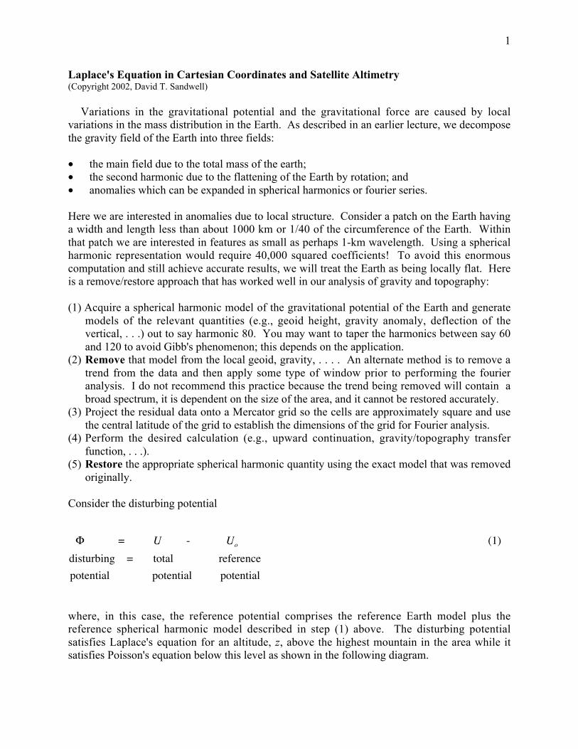
where, in this case, the reference potential comprises the reference Earth model plus thereference spherical harmonic model described in step (1) above. The disturbing potentialsatisfies Laplace's equation for an altitude, z, above the highest mountain in the area while itsatisfies Poisson's equation below this level as shown in the following diagram.

2

Φ(x,y,z) -- disturbing potential (total - reference)G -- gravitational constantρ -- density anomaly (total - reference)

Laplace's equation is a second order partial differential equation in three dimensions.

∂ 2Φ∂x2 + ∂ 2Φ

∂y2 + ∂ 2Φ∂z2 = 0, z > 0 (2)

Six boundary conditions are needed to develop a unique solution. Far from the region, thedisturbing potential must go to zero; this accounts for 5 of the boundary conditions

At the surface of the earth (or at some elevation), one must either prescribe the potential or thevertical derivative of the potential.

To solve this differential equation, we'll use the 2-D fourier transform again where the forwardand inverse transform are

Φ(x,y,0)=Φo(x,y) -- Dirichlet

∂Φ∂z

= − Δg(x,y) -- Neumann (4)

limx→∞

Φ = 0, limy→∞

Φ = 0, limz→∞

Φ = 0 (3)

z

∇2Φ = 0 air

y

x

∇2Φ = −4πGρ rock

3

F(k) = f (x−∞

∞

∫−∞

∞

∫ )e−i 2π (k ⋅x )d2x (5)

f (x) = F(k−∞

∞

∫−∞

∞

∫ )ei2π (k ⋅x)d2k

where x = (x, y) is the position vector, k = (1/λx,1/ λy) is the wavenumber vector, and

kix = kxx + kyy . Fourier transformation reduces Laplace's equation and the surface boundary to

−4π 2 kx2 + ky

2( )Φ(k,z ) + ∂ 2Φ∂z2 = 0 (6)

limz→∞

Φ(k,z) = 0, Φ(k,0) = Φo (7)

The general solution is

Φ(k, z) = A(k)e2π k z + B(k)e−2π k z (8)

To satisfy the boundary condition as z→ ∞ , the A(k) term must be zero. To satisfy theboundary condition on the z=0 plane, B(k) must be Φ(k,0). The final result is

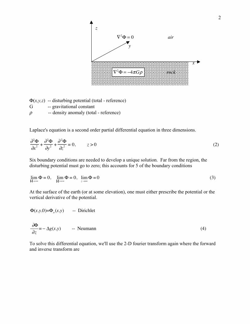
Φ(k, z) = Φo (k,0) e−2π k z (9)

potential at = potential at × upwardaltitude z = 0 continuation

Figure 1. Gain of upwardcontinuation kernel as a function ofthe altitude of the observation z,divided by the wavelength of theanomaly λ.

4

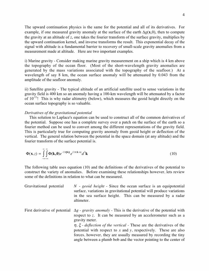
The upward continuation physics is the same for the potential and all of its derivatives. Forexample, if one measured gravity anomaly at the surface of the earth Δg(x,0), then to computethe gravity at an altitude of z, one takes the fourier transform of the surface gravity, multiplies bythe upward continuation kernel, and inverse transforms the result. This exponential decay of thesignal with altitude is a fundamental barrier to recovery of small-scale gravity anomalies from ameasurement made at altitude. Here are two important examples.

i) Marine gravity - Consider making marine gravity measurement on a ship which is 4 km abovethe topography of the ocean floor. (Most of the short-wavelength gravity anomalies aregenerated by the mass variations associated with the topography of the seafloor.) At awavelength of say 8 km, the ocean surface anomaly will be attenuated by 0.043 from theamplitude of the seafloor anomaly.

ii) Satellite gravity - The typical altitude of an artificial satellite used to sense variations in thegravity field is 400 km so an anomaly having a 100-km wavelength will be attenuated by a factorof 10-11! This is why radar altimetry (below), which measures the geoid height directly on theocean surface topography is so valuable.

Derivatives of the gravitational potentialThis solution to Laplace's equation can be used to construct all of the common derivatives of

the potential. Suppose one has a complete survey over a patch on the surface of the earth so afourier method can be used to convert among the different representations of the gravity field.This is particularly true for computing gravity anomaly from geoid height or deflection of thevertical. The general relation between the potential in the space domain (at any altitude) and thefourier transform of the surface potential is.

Φ(x,z) = Φ(k,0−∞

∞

∫−∞

∞

∫ )e−2π k z ei 2π (k⋅x)d2k (10)

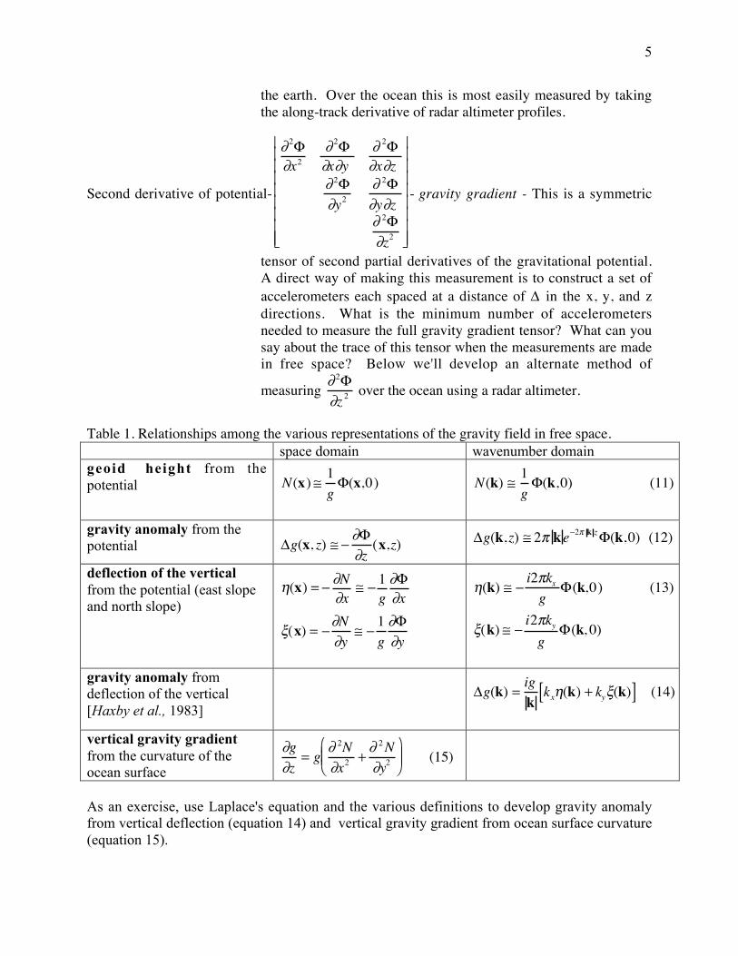
The following table uses equation (10) and the definitions of the derivatives of the potential toconstruct the variety of anomalies. Before examining these relationships however, lets reviewsome of the definitions in relation to what can be measured.

Gravitational potential N - geoid height - Since the ocean surface is an equipotentialsurface, variations in gravitational potential will produce variationsin the sea surface height. This can be measured by a radaraltimeter.

First derivative of potential Δg - gravity anomaly - This is the derivative of the potential withrespect to z. It can be measured by an accelerometer such as agravity meter.η, ξ - deflection of the vertical - These are the derivatives of thepotential with respect to x and y, respectively. These are alsoforces, however, they are usually measured by recording the tinyangle between a plumb bob and the vector pointing to the center of

5

the earth. Over the ocean this is most easily measured by takingthe along-track derivative of radar altimeter profiles.

Second derivative of potential-

∂ 2Φ∂x2

∂ 2Φ∂x∂y

∂ 2Φ∂x∂z

∂ 2Φ∂y2

∂ 2Φ∂y∂z∂ 2Φ∂z2

⎡

⎣

⎢ ⎢ ⎢ ⎢ ⎢ ⎢ ⎢ ⎢

⎤

⎦

⎥ ⎥ ⎥ ⎥ ⎥ ⎥ ⎥ ⎥

- gravity gradient - This is a symmetric

tensor of second partial derivatives of the gravitational potential.A direct way of making this measurement is to construct a set ofaccelerometers each spaced at a distance of Δ in the x, y, and zdirections. What is the minimum number of accelerometersneeded to measure the full gravity gradient tensor? What can yousay about the trace of this tensor when the measurements are madein free space? Below we'll develop an alternate method of

measuring ∂2Φ∂z 2

over the ocean using a radar altimeter.

Table 1. Relationships among the various representations of the gravity field in free space.space domain wavenumber domain

geoid height from thepotential N(x) ≅ 1

gΦ(x,0) N(k) ≅ 1

gΦ(k,0) (11)

gravity anomaly from thepotential Δg(x, z) ≅ − ∂Φ

∂z(x,z) Δg(k,z) ≅ 2π ke−2π k zΦ(k,0) (12)

deflection of the verticalfrom the potential (east slopeand north slope)

η(x) = − ∂N∂x

≅ − 1g∂Φ∂x

ξ(x) = −∂N∂y

≅ −1g∂Φ∂y

η(k) ≅ −i2πkxg

Φ(k,0) (13)

ξ(k) ≅ −i2πkyg

Φ(k, 0)

gravity anomaly fromdeflection of the vertical[Haxby et al., 1983]

Δg(k) = igkkxη(k) + kyξ(k)[ ] (14)

vertical gravity gradientfrom the curvature of theocean surface

∂g∂z

= g ∂ 2N∂x2 +

∂ 2N∂y2

⎛

⎝ ⎜ ⎜

⎞

⎠ ⎟ ⎟ (15)

As an exercise, use Laplace's equation and the various definitions to develop gravity anomalyfrom vertical deflection (equation 14) and vertical gravity gradient from ocean surface curvature(equation 15).

6

Here is a practical example. Suppose one has measurements of geoid height N(x)over a largearea on the surface of the ocean and we wish to calculate the gravity anomaly, Δg(x,z) at altitude.The prescription is:

(1) remove an appropriate spherical harmonic model from the geoid;(2) take the 2-D fourier transform of Ν(x);(3) multiply by g2π ke−2π k ;(4) take inverse 2-D fourier transform;(5) restore the matching gravity anomaly calculated from the spherical harmonic model at

altitude.

Conversion of geoid height to vertical deflection, gravity anomaly, and vertical gravitygradient from satellite altimeter profiles

As described above, geoid height N(x) and other measurable quantities such as gravityanomaly g(x) are related to the anomalous gravitational potential Φ(x,z) through Laplace'sequation. It is instructive to go through an example of how measurements of ocean surfacetopography from satellite altimetry can be used to construct geoid height, deflection of thevertical, gravity anomaly, and vertical gravity gradient.

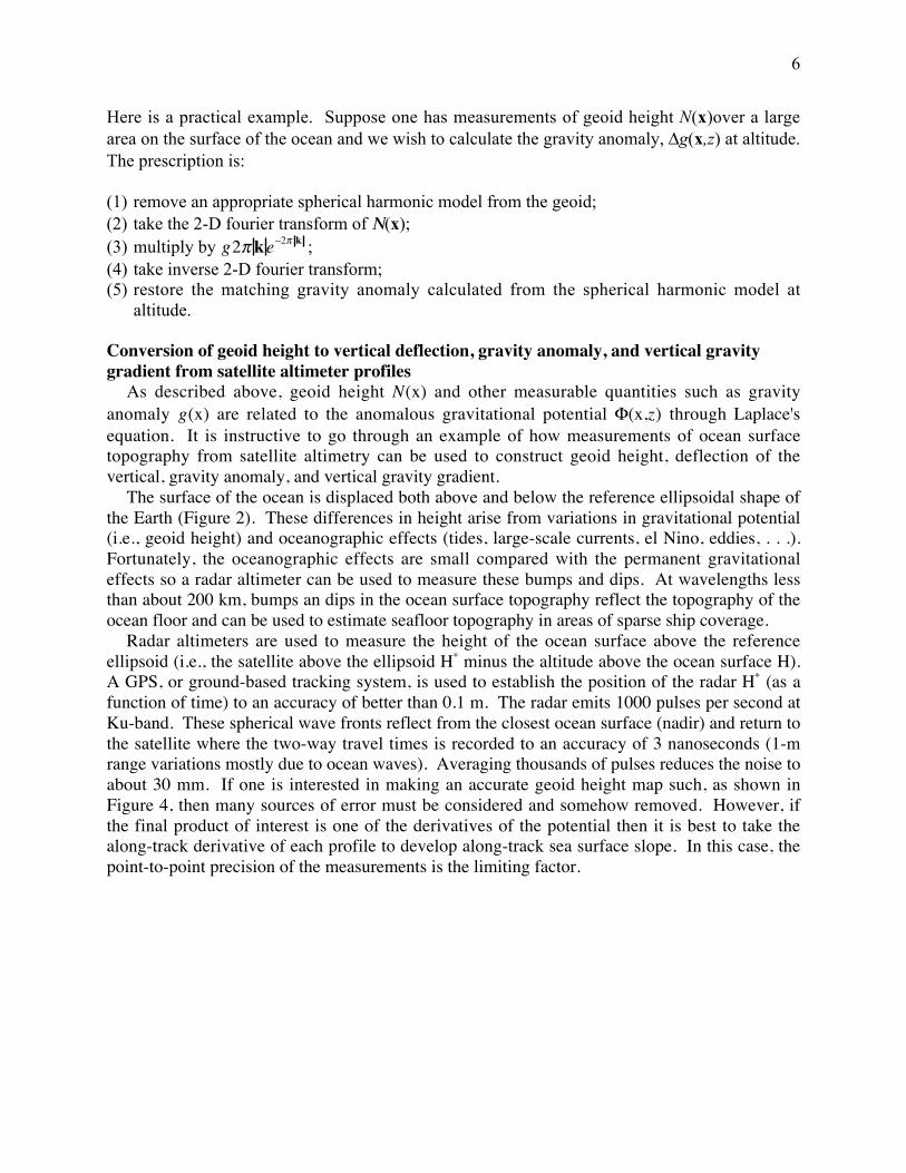
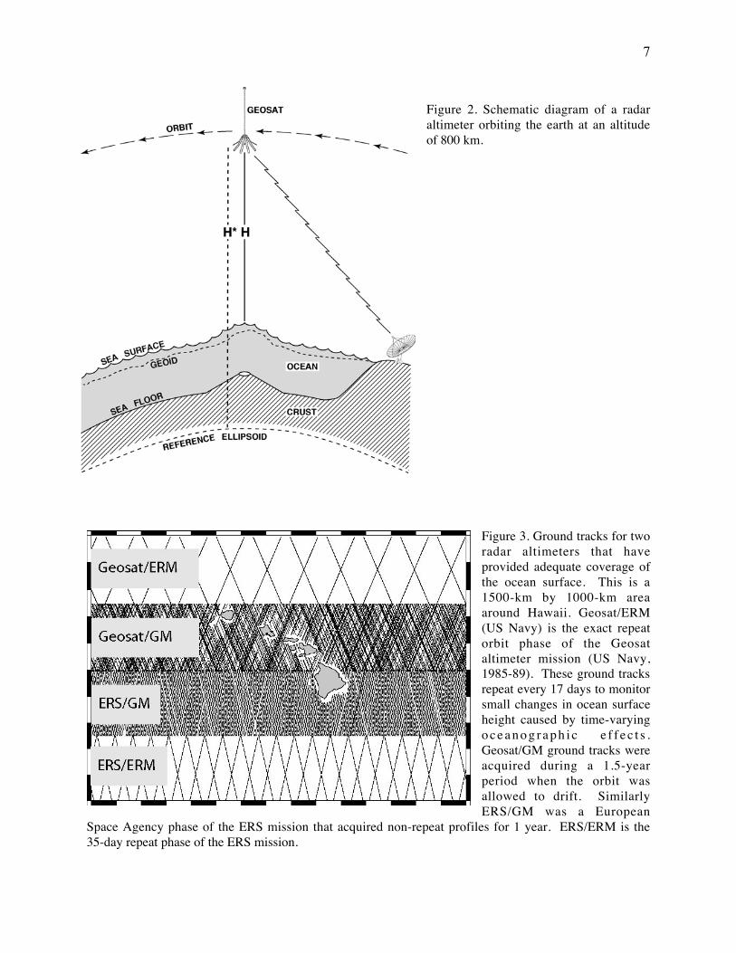
The surface of the ocean is displaced both above and below the reference ellipsoidal shape ofthe Earth (Figure 2). These differences in height arise from variations in gravitational potential(i.e., geoid height) and oceanographic effects (tides, large-scale currents, el Nino, eddies, . . .).Fortunately, the oceanographic effects are small compared with the permanent gravitationaleffects so a radar altimeter can be used to measure these bumps and dips. At wavelengths lessthan about 200 km, bumps an dips in the ocean surface topography reflect the topography of theocean floor and can be used to estimate seafloor topography in areas of sparse ship coverage.

Radar altimeters are used to measure the height of the ocean surface above the referenceellipsoid (i.e., the satellite above the ellipsoid H* minus the altitude above the ocean surface H).A GPS, or ground-based tracking system, is used to establish the position of the radar H* (as afunction of time) to an accuracy of better than 0.1 m. The radar emits 1000 pulses per second atKu-band. These spherical wave fronts reflect from the closest ocean surface (nadir) and return tothe satellite where the two-way travel times is recorded to an accuracy of 3 nanoseconds (1-mrange variations mostly due to ocean waves). Averaging thousands of pulses reduces the noise toabout 30 mm. If one is interested in making an accurate geoid height map such, as shown inFigure 4, then many sources of error must be considered and somehow removed. However, ifthe final product of interest is one of the derivatives of the potential then it is best to take thealong-track derivative of each profile to develop along-track sea surface slope. In this case, thepoint-to-point precision of the measurements is the limiting factor.

7

Figure 2. Schematic diagram of a radaraltimeter orbiting the earth at an altitudeof 800 km.

Figure 3. Ground tracks for tworadar altimeters that haveprovided adequate coverage ofthe ocean surface. This is a1500-km by 1000-km areaaround Hawaii. Geosat/ERM(US Navy) is the exact repeatorbit phase of the Geosataltimeter mission (US Navy,1985-89). These ground tracksrepeat every 17 days to monitorsmall changes in ocean surfaceheight caused by time-varyingo c e a n o g r a p h i c e f f e c t s .Geosat/GM ground tracks wereacquired during a 1.5-yearperiod when the orbit wasallowed to drift. SimilarlyERS/GM was a European

Space Agency phase of the ERS mission that acquired non-repeat profiles for 1 year. ERS/ERM is the35-day repeat phase of the ERS mission.

8

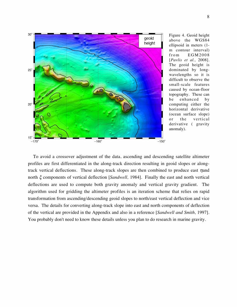
Figure 4. Geoid heightabove the WGS84ellipsoid in meters (1-m contour interval)f r o m E G M 2 0 0 8[Pavlis et al., 2008].The geoid height isdominated by long-wavelengths so it isdifficult to observe thesmall-scale featurescaused by ocean-floortopography. These canbe enhanced bycomputing either thehorizontal derivative(ocean surface slope)o r the ve r t i ca lderivative ( gravityanomaly).

To avoid a crossover adjustment of the data, ascending and descending satellite altimeterprofiles are first differentiated in the along-track direction resulting in geoid slopes or along-track vertical deflections. These along-track slopes are then combined to produce east η andnorth ξ components of vertical deflection [Sandwell, 1984]. Finally the east and north verticaldeflections are used to compute both gravity anomaly and vertical gravity gradient. Thealgorithm used for gridding the altimeter profiles is an iteration scheme that relies on rapidtransformation from ascending/descending geoid slopes to north/east vertical deflection and viceversa. The details for converting along-track slope into east and north components of deflectionof the vertical are provided in the Appendix and also in a reference [Sandwell and Smith, 1997].You probably don't need to know these details unless you plan to do research in marine gravity.

9

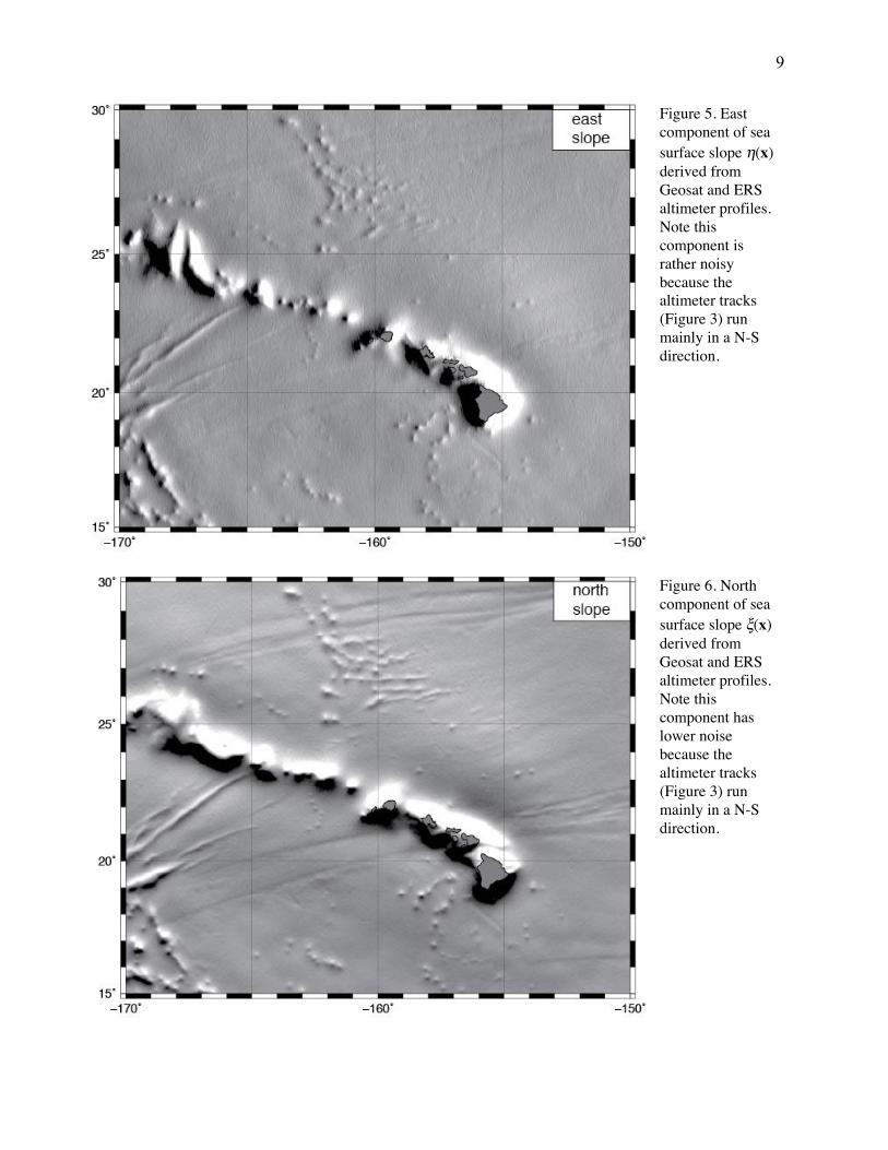
Figure 5. Eastcomponent of seasurface slope η(x)derived fromGeosat and ERSaltimeter profiles.Note thiscomponent israther noisybecause thealtimeter tracks(Figure 3) runmainly in a N-Sdirection.

Figure 6. Northcomponent of seasurface slope ξ(x)derived fromGeosat and ERSaltimeter profiles.Note thiscomponent haslower noisebecause thealtimeter tracks(Figure 3) runmainly in a N-Sdirection.

10

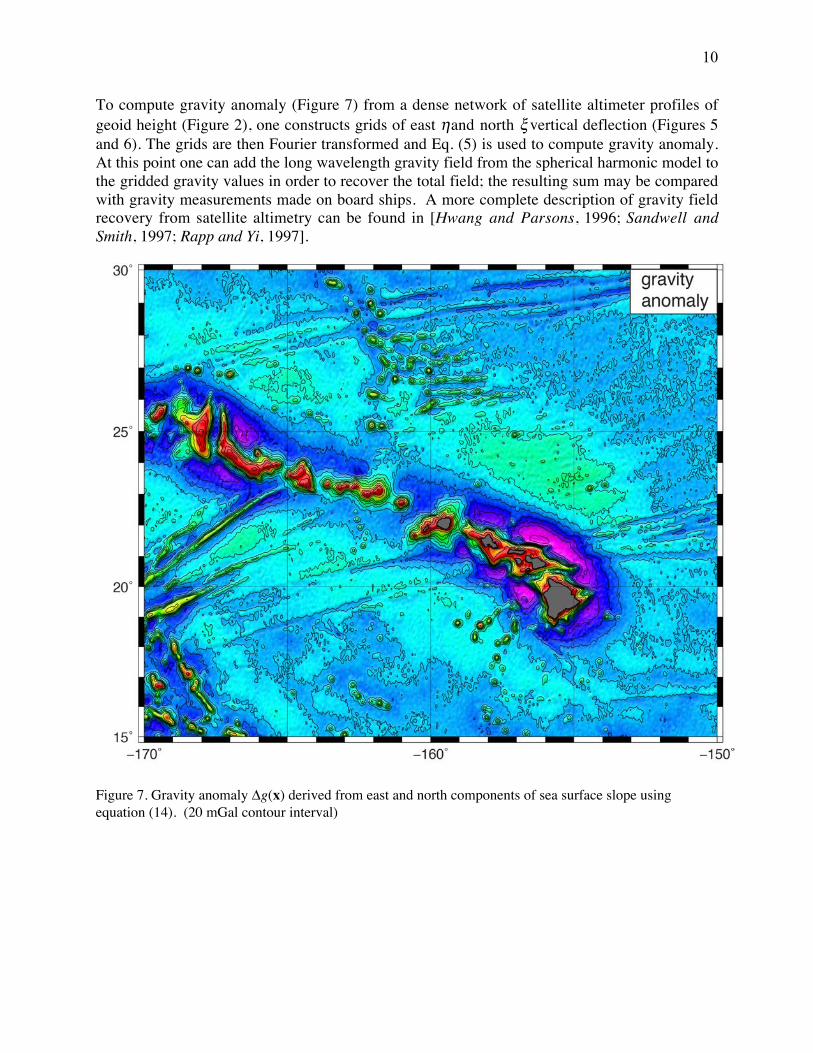
To compute gravity anomaly (Figure 7) from a dense network of satellite altimeter profiles ofgeoid height (Figure 2), one constructs grids of east η and north ξ vertical deflection (Figures 5and 6). The grids are then Fourier transformed and Eq. (5) is used to compute gravity anomaly.At this point one can add the long wavelength gravity field from the spherical harmonic model tothe gridded gravity values in order to recover the total field; the resulting sum may be comparedwith gravity measurements made on board ships. A more complete description of gravity fieldrecovery from satellite altimetry can be found in [Hwang and Parsons, 1996; Sandwell andSmith, 1997; Rapp and Yi, 1997].

Figure 7. Gravity anomaly Δg(x) derived from east and north components of sea surface slope usingequation (14). (20 mGal contour interval)

11

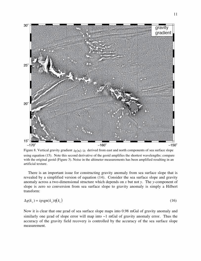
Figure 8. Vertical gravity gradient ∂g x( ) / ∂z derived from east and north components of sea surface slopeusing equation (15). Note this second derivative of the geoid amplifies the shortest wavelengths; comparewith the original geoid (Figure 3). Noise in the altimeter measurements has been amplified resulting in anartificial texture.

There is an important issue for constructing gravity anomaly from sea surface slope that isrevealed by a simplified version of equation (14). Consider the sea surface slope and gravityanomaly across a two-dimensional structure which depends on x but not y. The y-component ofslope is zero so conversion from sea surface slope to gravity anomaly is simply a Hilberttransform:

Δg(kx ) = igsgn(kx)η kx( ) (16)

Now it is clear that one µrad of sea surface slope maps into 0.98 mGal of gravity anomaly andsimilarly one µrad of slope error will map into ~1 mGal of gravity anomaly error. Thus theaccuracy of the gravity field recovery is controlled by the accuracy of the sea surface slopemeasurement.

12

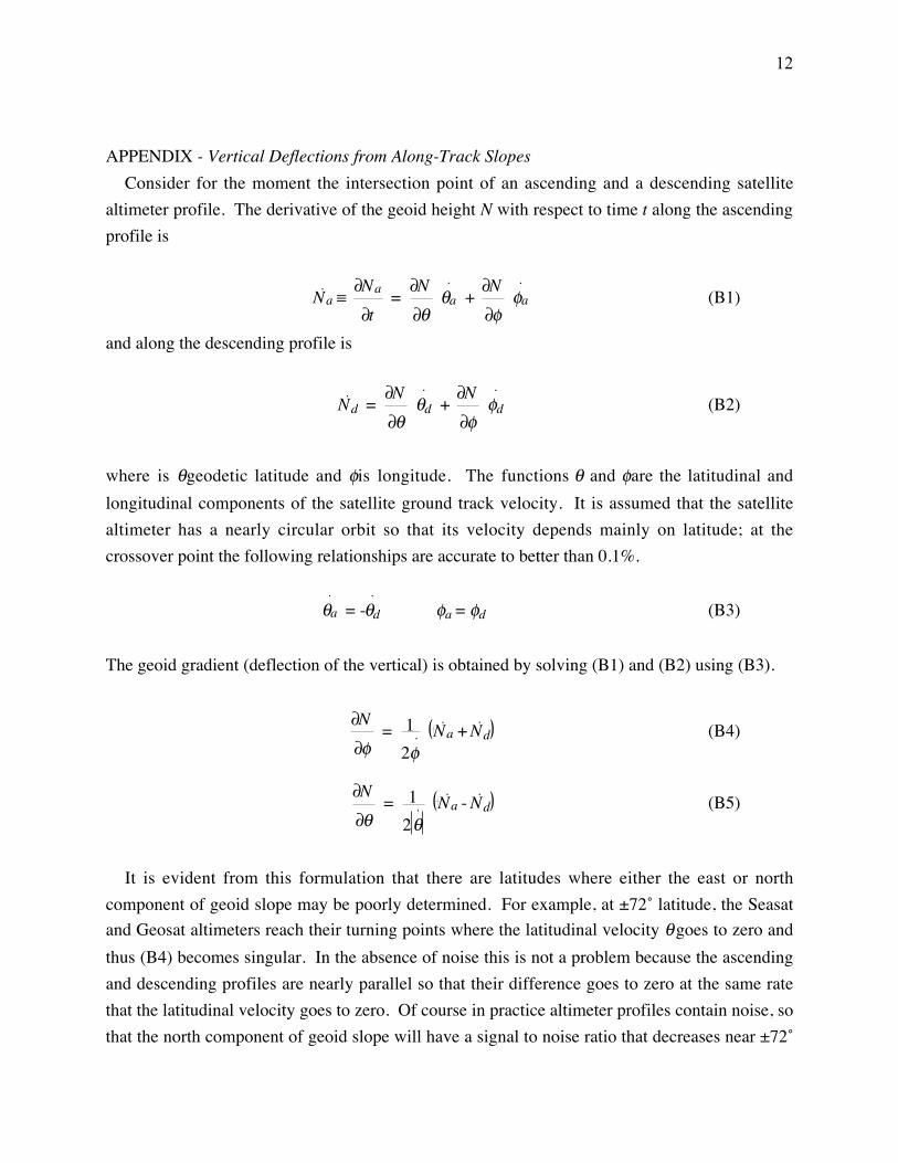
APPENDIX - Vertical Deflections from Along-Track SlopesConsider for the moment the intersection point of an ascending and a descending satellite

altimeter profile. The derivative of the geoid height N with respect to time t along the ascendingprofile is

Na ≡ ∂Na

∂t = ∂N

∂θ θa +

∂N∂φ

φa (B1)

and along the descending profile is

Nd = ∂N∂θ

θd + ∂N∂φ

φd (B2)

where is θ geodetic latitude and φ is longitude. The functions θ and φ are the latitudinal andlongitudinal components of the satellite ground track velocity. It is assumed that the satellitealtimeter has a nearly circular orbit so that its velocity depends mainly on latitude; at thecrossover point the following relationships are accurate to better than 0.1%.

θa = -θd φa = φd (B3)

The geoid gradient (deflection of the vertical) is obtained by solving (B1) and (B2) using (B3).

∂N∂φ

= 12φ

Na + Nd (B4)

∂N∂θ

= 12θ

Na - Nd (B5)

It is evident from this formulation that there are latitudes where either the east or northcomponent of geoid slope may be poorly determined. For example, at ±72˚ latitude, the Seasatand Geosat altimeters reach their turning points where the latitudinal velocity θ goes to zero andthus (B4) becomes singular. In the absence of noise this is not a problem because the ascendingand descending profiles are nearly parallel so that their difference goes to zero at the same ratethat the latitudinal velocity goes to zero. Of course in practice altimeter profiles contain noise, sothat the north component of geoid slope will have a signal to noise ratio that decreases near ±72˚

13

latitude. Similarly for an altimeter in a near polar orbit, the ascending and descending profilesare nearly anti-parallel at the low latitudes; the east component of geoid slope is poorlydetermined and the north component is well determined. The optimal situation occurs when thetracks are nearly perpendicular so that the east and north components of geoid slope have thesame signal to noise ratio.

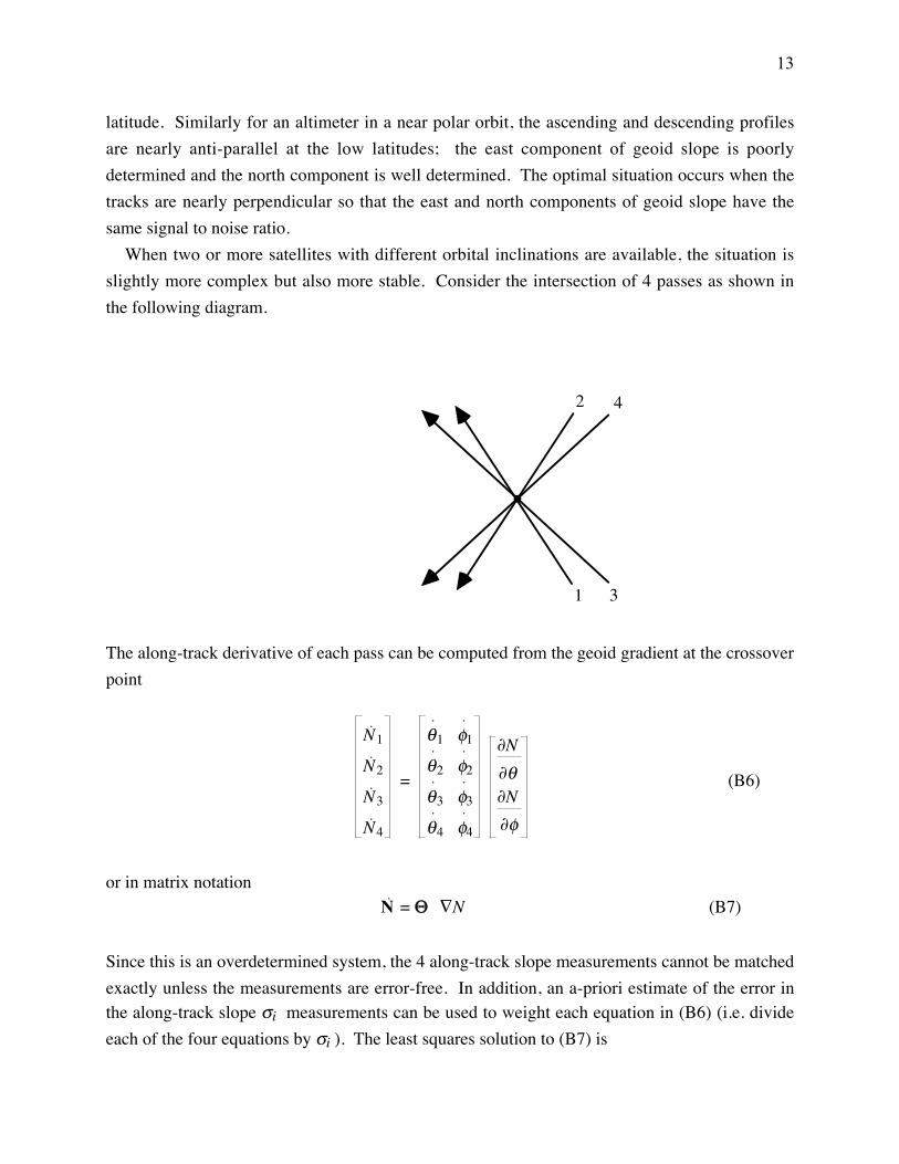
When two or more satellites with different orbital inclinations are available, the situation isslightly more complex but also more stable. Consider the intersection of 4 passes as shown inthe following diagram.

1 3

2 4

The along-track derivative of each pass can be computed from the geoid gradient at the crossoverpoint

N1

N2

N3

N4

=

θ1 φ1θ2 φ2θ3 φ3θ4 φ4

∂N∂θ∂N∂φ

(B6)

or in matrix notationN = Θ ∇N (B7)

Since this is an overdetermined system, the 4 along-track slope measurements cannot be matchedexactly unless the measurements are error-free. In addition, an a-priori estimate of the error inthe along-track slope σi measurements can be used to weight each equation in (B6) (i.e. divideeach of the four equations by σi ). The least squares solution to (B7) is

14

∇N = Θt Θ-1Θt N (B8)

where t and -1 are the transpose and inverse operations, respectively. In this case a 2 by 4system must be solved at each crossover point although the method is easily extended to three ormore satellites. Later we will assume that every grid cell corresponds to a crossover point of allthe satellites considered so this small system must be solved many times.

In addition to the estimates of geoid gradient, the covariances of these estimates are alsoobtained

σθθ2 σθφ

2

σφθ2 σφφ

2 = (ΘtΘ)-1

(B9)

Since Geosat and ERS-1 are high inclination satellites, the estimated uncertainty of the eastcomponent is about 3 times greater than the estimated uncertainty of the north component at theequator. At higher latitudes of 60˚-70˚ where the tracks are nearly perpendicular, the north andeast components are equally well determined. At 72˚ north where the Geosat tracks run in awesterly direction, the uncertainty of the east component is low and the higher inclination ERS-1tracks prevent the estimate of the north component from becoming singular at 72˚.

Finally, the east η and north ξ components of vertical deflection are related to the two geoidslopes by

η = - 1a cos θ

∂N∂φ

(B10)

ξ = - 1a ∂N∂θ

(B11)

where a is the mean radius of the earth.

REFERENCES

Haxby, W. F., Karner, G. D., LaBrecque, J. L., and Weissel, J. K. (1983). Digital images of

combined oceanic and continental data sets and their use in tectonic studies. EOS Trans.

Amer. Geophys. Un. 64, 995-1004.

Hwang, C., and Parsons, B. (1996). An optimal procedure for deriving marine gravity from

multi-satellite altimetry. J. Geophys. Int. 125, 705-719.

15

Pavlis, N. K., S. A. Holmes, S.C. Kenyon, and J.K. Factor, (2008) An Earth Gravitational Model

do Degree 2160: EGM2008, presented at the 2008 General Assembly of the European

Geosciences Union, Vienna, Austria, April 13-18.

Rapp, R. H., and Yi, Y. (1997). Role of ocean variability and dynamic topography in the

recovery of the mean sea surface and gravity anomalies from satellite altimeter data. J.

Geodesy 71, 617-629.

Sandwell, D. T. (1984). A detailed view of the South Pacific from satellite altimetry. J.

Geophys. Res. 89, 1089-1104.

Sandwell, D. T., and Smith, W. H. F. (1997). Marine gravity anomaly from Geosat and ERS-1

satellite altimetry. J. Geophys. Res. 102, 10,039-10,054.

Yale, M. M., D. T. Sandwell, and W. H. F. Smith, Comparison of along-track resolution of

stacked Geosat, ERS-1 and TOPEX satellite altimeters, J. Geophys. Res., 100, p. 15117-

15127, 1995.