Embed Size (px)
Citation preview
Adv. Appl. Prob. 40, 1048–1071 (2008)Printed in Northern Ireland
© Applied Probability Trust 2008
LARGE DEVIATIONS FOR EIGENVALUESOF SAMPLE COVARIANCE MATRICES,WITH APPLICATIONS TO MOBILECOMMUNICATION SYSTEMS
ANNE FEY,∗ Delft University of Technology
REMCO VAN DER HOFSTAD,∗∗ Eindhoven University of Technology
MARTEN J. KLOK,∗∗∗ Delft University of Technology
Abstract
We study sample covariance matrices of the form W = (1/n)CC�, where C is a k × n
matrix with independent and identically distributed (i.i.d.) mean 0 entries. This is ageneralization of the so-called Wishart matrices, where the entries of C are i.i.d. standardnormal random variables. Such matrices arise in statistics as sample covariance matrices,and the high-dimensional case, when k is large, arises in the analysis of DNA experiments.We investigate the large deviation properties of the largest and smallest eigenvalues ofW when either k is fixed and n → ∞ or kn → ∞ with kn = o(n/log log n), in thecase where the squares of the i.i.d. entries have finite exponential moments. Previousresults, proving almost sure limits of the eigenvalues, require only finite fourth moments.Our most explicit results for large k are for the case where the entries of C are ±1 withequal probability. We relate the large deviation rate functions of the smallest and largesteigenvalues to the rate functions for i.i.d. standard normal entries of C. This case is ofparticular interest since it is related to the problem of decoding of a signal in a code-division multiple-access (CDMA) system arising in mobile communication systems. Inthis example, k is the number of users in the system and n is the length of the codingsequence of each of the users. Each user transmits at the same time and uses the samefrequency; the codes are used to distinguish the signals of the separate users. The resultsimply large deviation bounds for the probability of a bit error due to the interference ofthe various users.
Keywords: Sample covariance matrix; large deviation; eigenvalue; CDMA with soft-decision parallel interference cancellation
2000 Mathematics Subject Classification: Primary 60F10; 62H20; 94A99
1. Introduction
The sample covariance matrix W of a matrix C with k rows and n columns is defined as(1/n)CC�. If C has random entries then the spectrum of W is random as well. Typically, W isstudied in the case that C has independent and identically distributed (i.i.d.) entries, with mean0 and variance 1. For this kind of C, it is known that, when k, n → ∞ such that k/n = β, where
Received 8 June 2007; revision received 10 November 2008.∗ Postal address: DIAM, Delft University of Technology, Mekelweg 4, 2628 CD Delft, The Netherlands.Email address: [email protected]∗∗ Postal address: Department of Mathematics, Eindhoven University of Technology, PO Box 513, 5600 MBEindhoven, The Netherlands. Email address: [email protected]∗∗∗ Current address: ORTEC BV, Orlyplein 145c, 1043 DV Amsterdam, The Netherlands.Email address: [email protected]
1048
Large deviations for eigenvalues of sample covariance matrices 1049
β is a constant, the eigenvalue density tends to a deterministic density [14]. The boundariesof the support of this distribution are (1 − √
β)2+ and (1 + √β)2, where x+ = max{0, x}.
This suggests that the smallest eigenvalue, λmin, converges to (1 − √β)2+, while the largest
eigenvalue, λmax, converges to (1 +√β)2. Bai andYin [3] proved the almost sure convergence
of λmin to (1 − √β)2+. Bai et al. [4] proved the almost sure convergence of λmax to (1 + √
β)2;see also [23]. The strongest results apply in the case that all the entries of C are i.i.d. with mean0, variance 1, and finite fourth moment. Related results, including a central limit theorem forthe linear spectral statistics, can be found in [1] and [2], to which we also refer for an overviewof the extensive literature.
In the special case that the entries of C have a standard normal distribution, W is calleda Wishart matrix. Wishart matrices play an important role in multivariate statistics as theydescribe the correlation structure in i.i.d. Gaussian multivariate data. For Wishart matrices, thelarge deviation rate function for the eigenvalue density with rate 1/n2 has been derived in [10]and [12]. However, the proofs heavily depend on the fact that C has standard normal i.i.d.entries, for which the density of the ordered eigenvalues can be explicitly computed.
In this paper we investigate the large deviation rate functions with rate 1/n of the smallestand largest eigenvalues of W for certain non-Gaussian entries of C. We pose a strong conditionon the tails of the entries, by requiring that the exponential moment of the square of the entriesis bounded in a neighborhood of the origin. We will also comment on this assumption, whichwe believe to be necessary for our results to apply.
We let n → ∞, and k is either fixed or tends to ∞ not faster than o(n/log log n). Ourresults imply that all eigenvalues tend to 1 and that all other values are large deviations. Weobtain the asymptotic large deviation rate function of λmin and λmax when k → ∞. In certainspecial cases we can show that the asymptotic large deviation rate function is equal to the onefor Wishart matrices, which can be interpreted as saying that the spectrum of sample covariancematrices with large k and n is close to the one for i.i.d. standard normal entries. This proves akind of universality result for the large deviation rate functions.
This paper is organized as follows. In Section 2 we derive an explicit expression for the largedeviation rate functions of λmin and λmax. In Section 3 we calculate lower bounds for the casein which the distribution of Cmi is symmetric around 0 and |Cmi | < M almost surely (a.s.) forsome M > 0. In Section 4 we specialize to the case where Cmi = ±1 with equal probability,which arises in an application in wireless communication. We describe the implications ofour results in this application in Section 5. Part of the results for this application have beenpresented at an electrical engineering conference [8].
2. General mean 0 entries of C
In this section we prove large deviation results for the smallest and largest eigenvalues ofsample covariance matrices.
2.1. Large deviations for λmin and λmax
Define W = (1/n)CC� to be the matrix of sample covariances. We denote by P the lawof C and by E the corresponding expectation. Throughout the paper, we assume that the i.i.d.real matrix elements of C are normalized, i.e.
E[Cij ] = 0, var(Cij ) = 1. (2.1)
The former assumption implies that, a.s., the off-diagonal elements of the matrix W converge

1050 A. FEY ET AL.
to 0, the latter assumption implies that the diagonal elements converge to 1 a.s. By a rescalingargument, the second assumption is without loss of generality.
In this subsection we rewrite the probability for a large deviation of the largest and smallesteigenvalues of W , λmax and λmin, respectively, into that of a large deviation of a sum of i.i.d.random variables. This rewrite allows us to use Cramér’s theorem to obtain an expression forthe rate function. In this subsection we give a heuristic derivation of our result, which will beturned into a proof in Subsection 2.2.
For any matrix W , and any vector x with k coordinates and norm ‖x‖2 = 1, we have
λmin ≤ 〈x, Wx〉 ≤ λmax,
where 〈x, y〉 denotes the inner product in Rk . Moreover, for the normalized eigenvector xmin
corresponding to λmin, the lower bound is attained, while for the normalized xmax correspondingto λmax, the upper bound is attained. Therefore, we can write
Pmin(α) = P(λmin ≤ α) = P(there exists x : ‖x‖2 = 1, 〈x, Wx〉 ≤ α),
Pmax(α) = P(λmax ≥ α) = P(there exists x : ‖x‖2 = 1, 〈x, Wx〉 ≥ α).
We use the fact that Pmin(α) and Pmax(α) are the probabilities of union of events, and boundthis probability from below by considering only one x and from above by summing over all x.Since there are uncountably many possible x, we will do this approximately by summing overa finite number of vectors. The lower bound for the probability yields an upper bound for therate function, and vice versa.
We first heuristically explain the form of the rate functions of λmax and λmin, and highlightthe proof. The special form of a sample covariance matrix allows us to rewrite
〈x, Wx〉 = 1
n‖C�x‖2
2 = 1
n
n∑i=1
( k∑m=1
xmCmi
)2
= 1
n
n∑i=1
S2x,i , (2.2)
where
Sx,i =k∑
m=1
xmCmi, (2.3)
with Sx,i i.i.d. for i = 1, . . . , m. Define
Ik(α) = infx∈Rk : ‖x‖2=1
supt
(tα − log E[exp{tS2x,1}]). (2.4)
Since E[S2x,1] = 1 and t �→ log E[exp{tS2
x,1}] is increasing and convex, we see that, for fixedx, the optimal t is nonnegative for α ≥ 1 and nonpositive for α ≤ 1. The sign of t will play animportant role in the proofs in Sections 3 and 4.
We can now state the first result of this paper.
Theorem 2.1. Assume that (2.1) holds. Then,
(a) for all α ≥ 1 and fixed k ≥ 2,
lim supn→∞
−1
nlog P(λmax ≥ α) ≤ Ik(α) (2.5)
and
lim infn→∞ −1
nlog P(λmax ≥ α) ≥ lim
ε↓0Ik(α − ε), (2.6)
Large deviations for eigenvalues of sample covariance matrices 1051
(b) for all 0 ≤ α ≤ 1 and fixed k ≥ 2,
lim supn→∞
−1
nlog P(λmin ≤ α) ≤ Ik(α) (2.7)
and
lim infn→∞ −1
nlog P(λmin ≤ α) ≥ lim
ε↓0Ik(α + ε). (2.8)
When there exists an ε > 0 such that E[exp{εC211}] < ∞ and when var(C2
11) > 0, thenIk(α) > 0 for all α �= 1.
We will now discuss the main result in Theorem 2.1. Theorem 2.1 is only useful whenIk(α) > 0, which we prove under the strong condition that there exists an ε > 0 such thatE[exp{εC2
11}] < ∞. For example, almost sure limits for the largest and smallest eigenvaluesare proved under the much weaker condition that the fourth moment of the matrix entries Cim
is finite. However, it is well known that the exponential bounds present in large deviationsare valid only when the random variables under consideration have finite exponential moments(see, e.g. Theorem 2.2, below). In this case, the rate functions can be equal to 0, and the largedeviation results are rather uninformative. Since the eigenvalues are quadratic in the entries{Cim}i,m, this translates into the above condition, which we therefore believe to be necessary.
Secondly, we note that, due to the occurrence of an infimum over x and a supremum overt , it is unclear whether the function α �→ Ik(α) is continuous. Clearly, when α �→ Ik(α) iscontinuous, the upper and lower bounds in (2.5) and (2.6), as well as the ones in (2.7) and (2.8),are equal. We will see that this is the case for Wishart matrices in Subsection 2.3. The functionα �→ Ik(α) can easily be seen to be increasing on [1, ∞) and decreasing on (0, 1], sinceα �→ supt (tα − log E[exp{tS2
x,1}]) has the same monotonicity properties for every fixed x, sothat the limits limε↓0 Ik(α + ε) and limε↓0 Ik(α − ε) exist as monotone limits. The continuityof α �→ Ik(α) is not obvious. For example, in the simplest case where Cij = ±1 with equalprobability, we know that the large deviation rate function is not continuous, since the largesteigenvalue is at most k. Therefore, P(λmax ≥ α) = 0 for any α > k, and if α �→ Ik(α) is therate function of λmax for α ≥ 1 then Ik(α) = ∞ for α > k. It remains an interesting problemto determine in what cases α �→ Ik(α) is continuous.
Finally, we only prove that Ik(α) > 0 for all α �= 1 when var(C211) > 0. By the normalization
that E[C11] = 0 and E[C211] = 1, this excludes only the case in which C11 = ±1 with equal
probability. This case will be investigated in more detail in Theorem 4.1, below, where we willalso prove a lower bound implying that Ik(α) > 0 for all α �= 1.
Let
Ik(α, β) = infx,y∈R
k : ‖x‖2=‖y‖2=1〈x,y〉=0
sups,t
(tα + sβ − log E[exp{tS2x,1 + sS2
y,1}]).
Our proof also reveals that, for all 0 ≤ β ≤ 1 and α ≥ 1,
lim supn→∞
−1
nlog P(λmax ≥ α, λmin ≤ β) ≥ Ik(α, β) (2.9)
and
limn→∞ −1
nlog P(λmax ≥ α, λmin ≤ β) ≤ lim
ε↓0Ik(α + ε, β − ε). (2.10)
1052 A. FEY ET AL.
For Wishart matrices, for which the entries of C are i.i.d. standard normal, the random variableSx,i has a standard normal distribution, so that we can explicitly calculate Ik(α). We willelaborate on this in Subsection 2.3. For the case in which Cmi = ±1 with equal probability,Theorem 2.1 and its proof have also appeared in [8].
2.2. Proof of Theorem 2.1(a) and (b)
In the proof we will repeatedly make use of the largest-exponent-wins principle. We firstgive a short explanation of this principle. This principle concerns the exponential rate of thesum of two (or more) probabilities. From this point, we will abbreviate ‘exponential rate ofa probability’ by ‘rate’. Because of the minus sign, a smaller rate I means a larger exponentand, thus, a larger probability. Thus, if, for two events E1 and E2, both depending on someparameter n, we have
P(E1) ∼ exp{−nI1} and P(E2) ∼ exp{−nI2},then
− limn→∞
1
nlog(P(E1) + P(E2)) ∼ min{I1, I2}. (2.11)
In words, the principle states that, as n → ∞, the smallest exponent (i.e. the largest rate) willbecome negligible. It also implies that
− limn→∞
1
nlog P(E1 ∪ E2) ∼ min{I1, I2}.
In the proof we will make essential use of Cramér’s theorem, which we state here for thesake of completeness.
Theorem 2.2. (Cramér’s theorem and the Chernoff bound.) Let (Xi)∞i=1 be a sequence of i.i.d.
random variables. Then, for all a ≥ E[X1],
− limn→∞
1
nlog P
(1
n
n∑i=1
Xi ≥ a
)= sup
t≥0(ta − log E[exp{tX1}]), (2.12)
while, for all a ≤ E[X1],
− limn→∞
1
nlog P
(1
n
n∑i=1
Xi ≤ a
)= sup
t≤0(ta − log E[exp{tX1}]). (2.13)
The upper bounds in (2.12) and (2.13) hold for every n. Furthermore, when E[exp{tX1}] < ∞for all t with |t | ≤ ε and some ε > 0, then the right-hand sides of (2.12) and (2.13) are strictlypositive for all a �= E[X1].
See, e.g. [15, Theorem 1.1 and Proposition 1.9] for this result, and see [6] and [7] for generalintroductions to large deviation theory.
For the proof of Theorem 2.1(a) and (b), we start by showing that Ik(α) > 0 for all α �= 1when there exists an ε > 0 such that E[exp{εC2
11}] < ∞ and when var(C211) > 0. For this, we
note that, by the Cauchy–Schwarz inequality and (2.3), for every x with ‖x‖2 = 1,
S2x,i ≤
k∑m=1
x2m
k∑m=1
C2mi =
k∑m=1
C2mi,

Large deviations for eigenvalues of sample covariance matrices 1053
so that E[exp{tS2x,i}] ≤ E[exp{tC2
11}]k < ∞ whenever there exists an ε > 0 such thatE[exp{εC2
11}] < ∞. Thus, uniformly in x with ‖x‖2 = 1, the random variables S2x,i have
bounded exponential moments for t ≤ ε. As a result, the Taylor expansion,
log E[exp{tS2x,i}] = t + t2
2var(S2
x,i ) + O(|t |3), (2.14)
holds uniformly in x with ‖x‖2 = 1. We compute, since E[S2x,i] = E[C2
11] = 1 and, for x with‖x‖2 = 1,
E[S4x,i] = 3
(∑m
x2m
)2
− 3∑m
x4m + E[C4
11]∑m
x4m = 3 − 3
∑m
x4m + E[C4
11]∑m
x4m,
that
var(S2x,i ) = 3 − 3
∑m
x4m + E[C4
11]∑m
x4m − 1 = 2 − 2
∑m
x4m + var(C2
11)∑m
x4m,
which is bounded, since, by assumption, E[exp{tC211}] < ∞. Furthermore,
∑m x4
m ∈ [0, 1]uniformly in x with ‖x‖2 = 1, so that, again uniformly in x with ‖x‖2 = 1, var(S2
x,i ) ≥min{2, var(C2
11)} > 0. We conclude that, for sufficiently small t , uniformly in x with ‖x‖2 = 1,and by ignoring higher-order Taylor expansion terms of t �→ log E[exp{tS2
x,i}] in (2.14), whichis allowed when |t | is sufficiently small,
log E[exp{tS2x,i}] ≤ t + t2 min{2, var(C2
11)}.In turn, this implies that, for |t | ≤ ε small, and uniformly in x with ‖x‖2 = 1,
Ik(α) ≥ infx∈Rk : ‖x‖2=1
sup|t |≤ε
(tα − log E[exp{tS2x,1}])
≥ infx∈Rk : ‖x‖2=1
sup|t |≤ε
(t (α − 1) − t2
2min{2, var(C2
11)})
> 0,
the latter bound holding for every α �= 1 when var(C211) > 0. This completes the proof
that Ik(α) > 0 for all α �= 1 when there exists an ε > 0 such that E[exp{εC211}] < ∞ and
var(C211) > 0.
We continue by proving (2.5)–(2.8). The proof for λmax is similar to the one for λmin, so wewill focus on the latter. To obtain the upper bound of the rate of (2.2), we use the fact that, forany x′ with ‖x′‖2 = 1,
P(λmin ≤ α) = P(there exists x : 〈x, Wx〉 ≤ α) ≥ P(〈x′, Wx′〉 ≤ α). (2.15)
Now insert (2.2). Since x′ is fixed, the S2x′,i are i.i.d. variables, and we can apply Cramér’s
theorem to obtain the upper bound for the rate function for fixed x′. This yields, for every x′,
−lim infn→∞
1
nlog P(λmin ≤ α) ≤ sup
t(tα − log E[exp{tS2
x′,1}]).
If we maximize the right-hand side over x′ then we arrive at Ik(α) as the upper bound, and wehave proved (2.7). The proof of (2.5) is identical.

1054 A. FEY ET AL.
We are left to prove the lower bounds in (2.6) and (2.8). For this, we wish to sum over allpossible x. We approximate the sphere ‖x‖2 = 1 by a finite set of vectors x(j) with ‖x(j)‖2 = 1,such that the distance between two of these vectors is at most d, and observe that
|〈x, Wx〉 − 〈x(j), Wx(j)〉| = |〈(x − x(j)), Wx〉 + 〈x(j), W (x − x(j))〉|= |〈x, W (x − x(j))〉 + 〈x(j), W (x − x(j))〉|≤ (‖x‖ + ‖x(j)‖)‖W‖‖x − x(j)‖≤ 2λmaxd.
We need λmax ≤ κk, where κ is some large enough constant, with sufficiently high proba-bility, which we will prove first. We have λmax ≤ TW , where TW is the trace of W , since W isnonnegative. Note that
TW = 1
n
n∑i=1
k∑m=1
C2mi.
Thus, TW is a sum of nk i.i.d. variables.Since E[exp{tC2
11}] < ∞ for all t ≤ ε, we can use Cramér’s theorem for TW . Therefore,for any κ , by the Chernoff bound,
P(TW > κk) ≤ exp{−nkIC2(κ)},where
IC2(a) = supt
(ta − log E[exp{tC211}]).
Since E[C211] = var(C11) = 1, we have IC2(κ) > 0 for any κ > 1. Therefore, by picking κ > 1
large enough, we can make kIC2(κ) arbitrarily large. If we take kIC2(κ) larger than Ik(α − ε),according to (2.11), this will not influence the result. (Note that, when Ik(α − ε) = ∞ for allε > 0, then we can also let kIC2(κ) tend to ∞ by taking κ → ∞.)
It follows that
P(λmin ≤ α) ≤ P(there exists x(j) : 〈x(j), Wx(j)〉 ≤ α + 2dκk) + P(TW > κk)
≤∑j
P(〈x(j), Wx(j)〉 ≤ α + 2dκk) + P(TW > κk)
≤ Nd supx(j)
P(〈x(j), Wx(j)〉 ≤ α + 2dκk) + P(TW > κk), (2.16)
where Nd is the number of vectors in the finite approximation of the sphere. The above boundis valid for every choice of κ , k, α, and d .
We write ε = 2dκk, and we will later let ε ↓ 0. Then, applying the largest-exponent-winsprinciple for κ > 0 large enough, as well as Cramér’s theorem together with (2.2), we arrive at
−lim supn→∞
1
nlog P(λmin ≤ α) ≥ inf
x(j)sup
t(t (α + ε) − log E[exp{tS2
x(j),1}])
+ lim infn→∞
1
nlog Nd
≥ Ik(α + ε) + lim infn→∞
1
nlog Nd.
Large deviations for eigenvalues of sample covariance matrices 1055
In a similar way, we obtain
−lim supn→∞
1
nlog P(λmax ≥ α) ≥ inf
x(j)sup
t(t (α − ε) − log E[exp{tS2
x(j),1}])
+ lim infn→∞
1
nlog Nd
≥ Ik(α − ε) + lim infn→∞
1
nlog Nd,
where we take d so small that α − ε > 0.A simple overestimation of Nd is obtained by first taking [−1, 1]k ⊂ R
k around the origin,and laying a grid on this cube with grid length 1/L. We then normalize the centers of thesecubes to have norm 1. The finite set of vectors consists of the centers of the small cubes ofwidth 2/L. In this case,
d ≤ 3√
k
Land Nd ≤ Lk. (2.17)
Indeed, the first bound follows since, for any vector x, there exists a center of a small cube forwhich all coordinates are at most 1/L away. Therefore, the distance to this center is at most√
k/L. Since x has norm 1, the norm of the center of the cube is between 1 − √k/L and
1 + √k/L, and we find that the distance of x to the normalized center of the small cube is at
most
d ≤√
k
L+
√k/L
1 − √k/L
≤ 3
√k
L,
when√
k/L ≤ 12 . For this choice, we have ε = 6κk3/2/L, which we can make small by taking
L large.We conclude that, for any L < ∞, limn→∞(1/n) log Nd = 0, so that, for any κ > 1
sufficiently large,
−lim supn→∞
1
nlog P(λmin ≤ α) ≥ Ik(α + ε)
and
−lim supn→∞
1
nlog P(λmax ≥ α) ≥ Ik(α − ε),
when the right-hand sides are finite. Since the above statement is true for any ε, we can takeε ↓ 0 by letting L ↑ ∞. When the right-hand sides are infinite, we conclude that the left-handsides can also be made arbitrarily large by letting L ↑ ∞. This completes the proof of (2.6)and (2.8).
To prove (2.9) and (2.10), we follow the above proof. We first note that the eigenvectorscorresponding to λmax and λmin are orthogonal. Therefore, we obtain
P(λmax ≥ α, λmin ≤ β) = P(there exists x, y : ‖x‖2 = ‖y‖2 = 1, 〈x, y〉 = 0,
〈x, Wx〉 ≥ α, 〈y, Wy〉 ≤ β).
We now proceed as above, and for the lower bound, we pick any x and y satisfying therequirements in the probability on the right-hand side. The upper bound is slightly harder. Forthis, we need to pick a finite approximation for the choices of x andy such that‖x‖2 = ‖y‖2 = 1and 〈x, y〉 = 0. We will now show that we can do this in such a way that the total number ofpairs {x(i), y(i,j)}i,j≥1 is bounded by N2
d , where Nd is as in (2.17).
1056 A. FEY ET AL.
We pick {x(i)}i≥1, as in the above proof. Then, for fixed x(i), we define a finite numberof y such that 〈x(i), y〉 = 0. For this, we consider, for fixed x(i), only those cubes of width1/L around an x(j) for some j that contain at least one element z having norm 1 and such that〈z, x(i)〉 = 0. Fix one such cube. If there are more such z in this cube around x(j) then we pickthe unique element that is closest to x(j). We denote this element by y(j,i). The set of theseelements y(j,i) will be denoted by {y(j,i)}i≥1. The finite subset of the set ‖x‖2 = ‖y‖2 = 1and 〈x, y〉 = 0 then consists of {x(i), y(i,j)}i,j≥1.
Clearly, every x and y with ‖x‖2 = ‖y‖2 = 1 and 〈x, y〉 = 0 can be approximated by apair x(j) and y(j,i) such that ‖x − x(j)‖2 ≤ d and ‖y − y(i,j)‖2 ≤ 2d. Then we can completethe proof as above.
2.3. Special case: Wishart matrices
To give an example, we consider Wishart matrices, for which Cij are i.i.d. standard normal.In this case we can compute Ik(α) and Ik(α, β) explicitly. To compute Ik(α), we note that, forany x such that ‖x‖2 = 1, Sx,1 is standard normal. Therefore,
E[exp{tS2x,1}] = 1√
1 − 2t,
so that
Ik(α) = supt
(tα − log
(1√
1 − 2t
)).
In order to compute Ik(α), we note that the maximization problem over t in supt (tα −log(1/
√1 − 2t)) is straightforward, and yields t∗ = 1
2 − 1/2α and Ik(α) = 12 (α − 1 − log α).
Note that Ik(α) is independent of k. In particular, we see that α �→ Ik(α) is continuous, whichleads us to the following corollary.
Corollary 2.1. Let Cij be independent standard normals. Then,
(a) for all α ≥ 1 and fixed k ≥ 2,
limn→∞ −1
nlog P(λmax ≥ α) = 1
2(α − 1 − log α),
(b) for all 0 ≤ α ≤ 1 and fixed k ≥ 2,
lim supn→∞
−1
nlog P(λmin ≤ α) = 1
2(α − 1 − log α).
We next turn to the computation of Ik(α, β). When x and y are such that ‖x‖2 = ‖y‖2 = 1and 〈x, y〉 = 0, then (Sx,1, Sy,1) are normally distributed. It can be easily seen that E[Sx,1] = 0and E[S2
x,1] = ‖x‖22 = 1, so that Sx,1 and Sy,1 are standard normal. Moreover, E[Sx,1Sy,1] =
〈x, y〉 = 0, so that (Sx,1, Sy,1) are in fact independent standard normal random variables.Therefore,
E[exp{tS2x,1 + sS2
y,1}] = E[exp{tS2x,1}] E[exp{sS2
y,1}] = 1√1 − 2t
1√1 − 2s
and, for α ∈ [0, 1] and β ≥ 1,
Ik(α, β) = sups,t
(tα + sβ − log
(1√
1 − 2t
)− log
(1√
1 − 2s
))= Ik(α) + Ik(β),

Large deviations for eigenvalues of sample covariance matrices 1057
so that the exponential rate of the probability that λmax ≥ α and λmin ≤ β is equal to theexponential rate of the product of the probabilities that λmax ≥ α and λmin ≤ β. This remarkableform of independence seems to be true only for Wishart matrices.
The above considerations lead to the following corollary.
Corollary 2.2. Let Cij be independent standard normals. Then,
limn→∞ −1
nlog P(λmax ≥ α, λmin ≤ β) = 1
2(α − 1 − log α) + 1
2(β − 1 − log β).
In the sequel we will, among other things, investigate cases where, for k → ∞, the ratefunction Ik(α) for general Cij converges to the Gaussian limit I∞(α) = 1
2 (α − 1 − log α).
3. Asymptotics for the eigenvalues for symmetric and bounded entries of C
In this section we investigate the case where Cmi is symmetric around 0 and |Cmi | < M < ∞a.s., or Cmi is standard normal. To emphasize the role of k, we will denote the law of W for agiven k by Pk . We define the extension to k = ∞ of Ik(α) to be
I∞(α) = infx∈�2(N) : ‖x‖2=1
supt
(tα − log E[exp{tS2x,1}]), (3.1)
where �2(N) is the space of all infinite square-summable sequences with norm
‖x‖2 =√√√√ ∞∑
i=1
x2i .
The main result in this section is the following theorem.
Theorem 3.1. Suppose that Cmi is symmetric around 0 and that |Cmi | < M < ∞ a.s., or Cmi
is standard normal. Then, for all kn → ∞ such that kn = o(n/log log n),
(a) for all α ≥ 1,
lim infn→∞ −1
nlog Pkn(λmax ≥ α) ≤ I∞(α) (3.2)
and
lim supn→∞
−1
nlog Pkn(λmax ≥ α) ≥ lim
ε↓0I∞(α − ε), (3.3)
(b) for all 0 < α ≤ 1,
lim infn→∞ −1
nlog Pkn(λmin ≤ α) ≤ I∞(α) (3.4)
and
lim infn→∞ −1
nlog Pkn(λmin ≤ α) ≥ lim
ε↓0I∞(α + ε). (3.5)
A version of this result has also been published in a conference proceeding [8] for the specialcase Cmi = ±1, each with probability 1
2 , and where the restriction on kn was kn = O(n/log n).Unfortunately, there is a technical error in the proof; we present the corrected proof below. Inorder to do so, we will rely on explicit lower bounds for Ik(α), α ≥ 1.
A priori, it is not obvious that the limit I∞(α) is strictly positive for α �= 1. However, in theexamples we will investigate later on, such as Cmi = ±1 with equal probability, we will seethat indeed I∞(α) > 0 for α �= 1. Possibly, such a result can be shown more generally.
The following proposition is instrumental in the proof of Theorem 3.1.

1058 A. FEY ET AL.
Proposition 3.1. Assume that Cmi is symmetric around 0 and that |Cmi | < M < ∞ a.s., orCmi is standard normal. Then, for all k, α ≥ M2, and x with ‖x‖2 = 1,
Pk(〈x, Wx〉 ≥ α) ≤ exp{−nJ k(α)},where
Jk(α) = 1
2
(α
M2 − 1 − logα
M2
).
In the case where Cmi = ±1, for which M > 1, we will present an improved version of thisbound, valid when α ≥ 1
2 , in Theorem 4.1, below.
3.1. Proof of Proposition 3.1
Throughout this proof, we fix x with ‖x‖2 = 1. We use (2.2) to bound, for every t ≥ 0 andk ∈ N, by the Markov inequality,
Pk(〈x, Wx〉 ≥ α) = Pk
(exp
{t
n∑i=1
S2x,i
}≥ entα
)≤ exp{−n(αt − log Ekn [exp{tS2
x,1}])}.
We claim that, for all 0 ≤ t ≤ 1/M2,
Ekn [exp{tS2x,i}] ≤ 1√
1 − 2M2t. (3.6)
In the case of Wishart matrices, for which Sx,i has a standard normal distribution, (3.6) holdswith equality for M = 1.
We first note that (3.6) is proven in [18, Section IV] for the case in which Cij = ±1 withequal probability. For any k and x, the bound is even valid for all − 1
2 ≤ t ≤ 12 . We now extend
the case where Cij = ±1 to the case where Cij is symmetric around 0 and satisfies |Cij | < M
a.s.We write Cij = AijC
∗ij , where Aij = |Cij | < M a.s. and C∗
ij = sgn(Cij ). Moreover, Aij
and C∗ij are independent, since Cij has a symmetric distribution around 0. Thus, we obtain
Sx,i = S∗Aix,i , where (Aix)j = Aijxj , and
S∗y,i =
k∑j=1
C∗ij yj .
For S∗y,i , we know that (3.6) is proven. Therefore,
Ek[exp{tS2Aix,i}] ≤ Ek
[1√
1 − 2t‖Aix‖22
]
for all t such that − 12 ≤ t‖Aix‖2 ≤ 1
2 a.s. When ‖x‖22 = 1, we have
0 ≤ ‖Aix‖2 < M a.s.
Therefore,
Ek[exp{tS2Aix,i}] ≤ 1√
1 − 2M2t‖x‖22
for all 0 ≤ tM2‖x‖22 ≤ 1
2 .
Large deviations for eigenvalues of sample covariance matrices 1059
Thus, we arrive at
Pk(〈x, Wx〉 ≥ α) ≤ exp
{−n
(sup
0≤t≤1/M2
(tα − log
1√1 − 2M2t
))}. (3.7)
Note that, since ‖x‖2 = 1, the bound is independent of x. Taking the maximum over t ofthe right-hand side of (3.7) yields t∗ = 1/2M2 − 1/2α, and inserting this value of t∗ into theright-hand side of (3.7) gives the result.
3.2. Proof of Theorem 3.1
The proof is similar to that of Theorem 2.1. For the proofs of (3.2) and (3.4), we again use(2.15), but now choose an x′ of which only the first k components are nonzero. This leads to,using the fact that kn → ∞, so that kn ≥ k for sufficiently large n,
lim infn→∞ −1
nlog Pkn(λmax ≥ α) ≤ sup
t(tα − log E[exp{tS2
x′,1}]).
Maximizing over all x′ of which only the first k components are nonzero leads to
lim infn→∞ −1
nlog Pkn(λmax ≥ α) ≤ Ik(α),
where this bound is valid for all k ∈ N. We next claim that
limk→∞ Ik(α) = I∞(α). (3.8)
For this, we first note that the sequence k �→ Ik(α) is nonincreasing and nonnegative, so that ithas a pointwise limit. Secondly, Ik(α) ≥ I∞(α) for all k, since the number of possible choicesof x in (3.1) is larger than the one in (2.4). Now it is not hard to see that limk→∞ Ik(α) = I∞(α),
by splitting into the two cases depending on whether the infimum over x in (3.1) is attained ornot. This completes the proof of (3.2) and (3.4).
For the proof of (3.3) and (3.5), we adapt the proof of (2.6) and (2.8). As in the proof ofTheorem 2.1(a)–(b), we wish to show that the terms (1/n) log Nd and 2dλmax vanish when wetake the logarithm of (2.16), divide by n, and let n → ∞. However, this time we wish to letkn → ∞ as well, for kn as large as possible. We will have kn = o(n) in mind.
The overestimation (2.17) can be improved using an upper bound for the number MR = N1/R
of spheres of radius 1/R needed to cover the surface of a k-dimensional sphere of radius 1[17]: when k → ∞,
MR = 4k√
kRk(log k + log log k + log R)
(1 + O
(1
log k
))≡ f (k, R)Rk. (3.9)
This bound is valid for R >√
k/(k − 1). Since we use small spheres this time, d ≤ 1/R.We can also improve the upper bound for λmax. For any �n > 1, which we will choose
appropriately later on, we split
Pmin(α) ≤ P(λmin ≤ α, λmax ≤ �n) + Pmax(�n),
Pmax(α) = P(α ≤ λmax ≤ �n) + Pmax(�n). (3.10)
We first give a sketch of the proof, omitting the details. The idea is that the first term ofthese expressions will yield the rate function I∞(α). The term Pmax(�n) has an exponential

1060 A. FEY ET AL.
rate which is O(�n) − O(kn log kn/n), and, since kn log kn/n = o(log n), can thus be madearbitrarily large by taking �n = K log n with K > 1 large enough. This means that we canchoose �n large enough to make this rate disappear according to the largest-exponent-winsprinciple, (2.11). We will need different choices of R for the two terms. We will now give thedetails of the proof.
We first bound Pmax(�n) in (3.10) using (2.16). In (2.16) we choose κ = M2. This leads to
Pmax(�n) ≤ MR supx
P(〈x, Wx〉 ≥ �n − 2dM2kn) + P(TW ≥ M2kn),
where the supremum over x runs over the centers of the small balls. Inserting (3.9), choosingR = kn, and using d ≤ 1/R, this becomes
Pmax(�n) ≤ f (kn, kn)kknn sup
xP(〈x, Wx〉 ≥ �n − 2M2) + P(TW ≥ M2kn).
Using Proposition 3.1, we find that
Pmax(�n) ≤ f (kn, kn)kknn exp
{−1
2n
(�n
M2 − 3 − log
(�n
M2 − 2
))}+ exp{−nknIC2
11(M2)}
= f (kn, kn) exp
{kn log kn − 1
2n
(�n
M2 − 3 − log
(�n
M2 − 2)
)}
+ exp{−nknIC211
(M2)}.We choose �n = K log n with K so large that
kn log kn
n<
1
4
(�n
M2 − 3 − log
(�n
M2 − 2
)).
Therefore, also using the fact that
f (kn, kn) = eo(n log n),
we obtain
Pmax(�n) ≤ exp
{− K
4M2 n log n(1 + o(1))
}+ exp{−nknIC2
11(M2)}. (3.11)
Next, we investigate the first term of (3.10). In this term we can use �n as the upper boundfor λmax. Therefore, again starting with (2.16), we obtain, for any R,
−1
nlog P(λmin ≤ α, λmax ≤ �n) ≥ −1
n
[log MR + sup
xlog P
(〈x, Wx〉 ≤ α + 2�n
R
)].
(3.12)For λmax, we get a similar expression. Inserting (3.9), we need to choose R again. This time wewish to choose R = Rn to increase in such a way that kn log Rn = o(n) and �n = K log n =o(Rn). For the latter, we need Rn � log n, so that we can satisfy only the first restriction whenkn = o(n/log log n). Then this is sufficient to make the term 2�n/Rn disappear as kn → ∞,and to make the term (1/n)(log MRn) = O(kn log Rn) be o(n), so that it also disappears.Therefore, for any R = Rn satisfying the above two restrictions,
−1
nlog P(λmin ≤ α, λmax ≤ �n) ≥ Ikn
(α + 2
�n
Rn
)+ o(1). (3.13)
Large deviations for eigenvalues of sample covariance matrices 1061
Similarly,
−1
nlog P(α ≤ λmax ≤ �n) ≥ Ikn
(α − 2
�n
Rn
)+ o(1).
Moreover, by the fact that �n = K log n = o(Rn), we have 2�n/Rn ≤ ε for all large enough n.By the monotonicity of α �→ Ikn(α) we then have
Ikn
(α + 2�n
Rn
)≥ Ikn(α + ε), Ikn
(α − 2�n
Rn
)≥ Ikn(α − ε). (3.14)
Since limk→∞ Ik(α) = I∞(α) (see (3.8)), putting (3.13), (3.14), and (3.11) together andapplying the largest-exponent-wins principle, (2.11), we see that the proof follows when
I∞(α ± ε) < min
{log n
K
4M2 , knIC211
(M2)
}. (3.15)
Both terms are increasing in n, as long as IC211
(M2) > 0. This is true for the C11 we consider:if C11 is symmetric around 0 such that |C11| < M < ∞ a.s., then IC2
11(M2) = ∞, and if Cmi
is standard normal then IC211
(M2) > 0.Therefore, (3.15) is true when n is large enough, when I∞(α ± ε) < ∞. On the other hand,
when I∞(α ± ε) = ∞, then we find that the exponential rates converge to ∞, as stated in (3.3)and (3.5). We conclude that, for every ε > 0,
lim infn→∞ −1
nlog Pkn(λmin ≤ α) ≥ I∞(α + ε)
and
lim infn→∞ −1
nlog Pkn(λmax ≥ α) ≥ I∞(α − ε),
and letting ε ↓ 0 completes the proof for every sequence kn such that kn = o(n/log log n). Theproof for λmax is identical to the above proof.
We believe that the above argument can be extended somewhat further, by making a furthersplit into K ′ log log n ≤ λmax ≤ K log n and λmax ≤ K ′ log log n, but we refrain from writingthis down.
3.3. The limiting rate for large k
In this subsection we investigate what happens when we take k large. In certain cases wecan show that the rate function, which depends on k, converges to the rate function for Wishartmatrices. This will be formulated in the following theorem.
Theorem 3.2. Assume that Cij satisfies (2.1) and, moreover, that φC(t) = E[exp{tC11}] ≤exp{t2/2} for all t . Then, for all α ≥ 1 and all k ≥ 2,
Ik(α) ≥ 12 (α − 1 − log α), (3.16)
and, for all α ≥ 1,lim
k→∞ Ik(α) = I∞(α) = 12 (α − 1 − log α). (3.17)
Finally, for all kn → ∞ such that kn = o(n/log log n) and α ≥ 1,
limn→∞ −1
nlog Pkn(λmax ≥ α) = 1
2(α − 1 − log α). (3.18)

1062 A. FEY ET AL.
Note that, in particular, Theorem 3.2 implies that I∞(α) = 12 (α − 1 − log α) > 0 for all
α > 1.Theorem 3.2 is a kind of universality result, and shows that, for large k, the rate functions
of certain sample covariance matrices converge to the rate functions for Wishart matrices. Anexample where φC(t) ≤ exp{t2/2} holds is when Cij = ±1 with equal probability. We willcall this example the Bernoulli case. A second example is the uniform random variable on[−√
3,√
3], for which the variance also equals 1. We will prove these bounds below.Of course, the relation φC(t) ≤ exp{t2/2} for random variables with mean 0 and variance 1
is equivalent to the statement that φC(t) ≤ exp{t2σ 2/2} for a random variable C with mean 0and variance σ 2. Thus, we will check the condition for uniform random variables on [−1, 1]and for the Bernoulli case. We will denote the moment generating functions by φU and φB .We start with φB , for which we have
φB(t) = cosh(t) =∞∑
n=0
t2n
(2n)! ≤∞∑
n=0
t2n
2nn! = exp
{t2
2
},
since (2n)! ≥ 2nn! for all n ≥ 0. The proof for φU is similar. Indeed,
φU(t) = sinh(t)
t=
∞∑n=0
t2n
(2n + 1)! ≤∞∑
n=0
t2n
6nn! = exp
{t2
6
}= exp
{t2σ 2
2
},
since now (2n + 1)! ≥ 6nn! for all n ≥ 0.
Proof of Theorem 3.2. Using Theorems 2.1 and 3.1, we claim that it suffices to prove that,uniformly for x with ‖x‖2 = 1 and t < 1,
E[exp{tS2x,i}] ≤ 1√
1 − 2t. (3.19)
We will prove (3.19) below, but first we prove Theorem 3.2, assuming that (3.19) holds.When (3.19) holds, then, using Theorem 3.1 and (2.4), it immediately follows that (3.16)
holds. Here we also use the fact that α �→ 12 (α − 1 − log α) is continuous, so that the limit
over ε ↓ 0 can be computed.To prove (3.17), we take x = (1/
√k)(1, . . . , 1), to obtain, with Sk = ∑k
i=1 Ci1,
Ik(α) ≤ supt
(tα − log E
[exp
{t
kS2
k
}]).
We claim that, when k → ∞, for all 0 ≤ t < 1,
E
[exp
{t
kS2
k
}]→ E[exp{tZ2}] = 1√
1 − 2t, (3.20)
where Z is a standard normal random variable. This implies the lower bound for Ik(α) and, thus,(3.17). Equation (3.18) follows in a similar way, also using the fact that α �→ 1
2 (α − 1 − log α)
is continuous.We complete the proof by showing that (3.19) and (3.20) hold. We start with (3.19). We
rewrite, for t ≥ 0,
E[exp{tS2x,i}] = E[exp{√2tZSx,i}] = E
[ k∏j=1
φC(√
2tZxj )
],
Large deviations for eigenvalues of sample covariance matrices 1063
where Z is a standard normal random variable. We now use the fact that φC(t) ≤ exp{t2/2} toarrive at
E[exp{tS2x,i}] ≤ E
[ k∏j=1
exp{tZ2x2j }
]= E[exp{tZ2}] = 1√
1 − 2t.
This completes the proof of (3.19). We proceed with (3.20). We use
E[exp{tS2k}] = E
[ k∏j=1
φC
(√2t
kZ
)].
We will use dominated convergence. By the assumption that φC(t) ≤ exp{t2/2}, we have
φC
(√2t
kZ
)≤ exp
{t
kZ2
}, so that
k∏j=1
φC
(√2t
kZ
)≤ exp{tZ2},
which has a finite expectation when t < 12 . Moreover,
∏kj=1 φC((2t/k)1/2z) converges to
exp{tz2} pointwise in z. Therefore, dominated convergence proves the claim in (3.20), andcompletes the proof.
4. The smallest eigenvalue for Cij = ±1
Unfortunately, we are not able to prove a similar result as in Theorem 3.2 for the smallesteigenvalue. In fact, as we will comment on in more detail in Subsection 4.2, we expect theresult to be false for the smallest eigenvalue, in particular, when α is small. There is oneexample where we can prove a partial convergence result, and that is when Cij = ±1 withequal probability. Indeed, in this case it was shown in [18, Section IV] that (3.19) holds for allt ≥ −1. This leads to the following result, which also implies that Ik(α) > 0 for α �= 1 in thecase where var(C2
11) = 0 (recall also Theorem 2.1).
Theorem 4.1. Assume that Cij = ±1 with equal probability. Then, for all α ≥ 12 and all
k ≥ 2,
Ik(α) ≥ 12 (α − 1 − log α), (4.1)
and, for all α ≥ 12 ,
I∞(α) = 12 (α − 1 − log α). (4.2)
Finally, for all 0 < α ≤ 12 ,
Ik(α) ≥ 12 (−α + log 2). (4.3)
Proof. The proofs of (4.1) and (4.2) are identical to the proof of Theorem 3.2, now assumingthat (3.19) holds for all t ≥ −1. Equation (4.3) follows since
Ik(α) ≥ infx : ‖x‖2=1
(−α
2− log E
[exp
{−1
2S2
x,i
}])
and the bound on the moment generating function in (3.19), which, as discussed above, holdsfor all t ≥ −1 when Cij = ±1 with equal probability, for t = −1.

1064 A. FEY ET AL.
4.1. Rate for the probability of one or more zero eigenvalues for Cij = ±1
In the above computations we obtain no control over the probability of a large deviation ofthe smallest eigenvalue, λmin. In this and the next subsection we investigate this problem forthe case in which Cij = ±1.
Proposition 4.1. Suppose that Cij = ±1 with equal probability. Then, for all 0 < l ≤ k − 1and any kn = O(nb) for some b,
limn→∞ −1
nlog Pkn(λ1 = · · · = λl = 0) = l log 2, (4.4)
where the λi denote eigenvalues of W arranged in increasing order.
Proof. The upper bound in (4.4) is simple, since, to have l eigenvalues equal to 0, we cantake the first l + 1 columns of C to be equal. For eigenvectors w of W ,
〈w, Ww〉 = 1
n〈w, CC�w〉 = 1
n‖C�w‖2
2,
we find that w is an eigenvector with eigenvalue 0 precisely when ‖C�w‖2 = 0. When the firstl + 1 columns of C are equal, there are l linearly independent vectors for which ‖C�w‖2 = 0,so that the multiplicity of the eigenvalue 0 is at least l. Moreover, the probability that the firstl + 1 columns of C are equal is equal to 2nl .
We prove the lower bound in (4.4) by induction by showing that
limn→∞ −1
nlog Pkn(λ1 = · · · = λl = 0) ≥ l log 2. (4.5)
When l = 0, the claim is trivial. It suffices to advance the induction hypothesis.Suppose that there are l linear independent eigenvectors with eigenvalue 0. Since the
eigenvectors can be chosen to be orthogonal, it is possible to make linear combinations, suchthat the first l − 1 eigenvectors all have one zero coordinate j , whereas the lth eigenvectorshas all zero coordinates except for coordinate j . This means that the first l − 1 eigenvectorsfix some part of C�, but not the j th column. The lth eigenvector however fixes precisely thiscolumn. Fixing one column of C� has probability 2−n. The number of possible rows j isbounded by k, which in turn is bounded by nb = eo(n). Therefore, we have
limn→∞ −1
nlog Pkn(λ1 = · · · = λl = 0)
≥ log 2 + limn→∞ −1
nlog Pkn(λ1 = · · · = λl−1 = 0).
The claim follows from the induction hypothesis.
Note that Proposition 4.1 shows that (4.2) cannot be extended to α = 0. Therefore, achangeover takes place between α = 0 and α ≥ 1
2 , where, for α ≥ 12 , the rate function equals
the one for Wishart matrices, while, for α = 0, this is not the case. We will comment more onthis in Conjecture 4.1, below.
4.2. A conjecture about the smallest eigenvalue for Cij = ±1
We have already shown that (4.1) is sharp. By Proposition 4.1, (4.3) is not sharp, sinceImin(0) = log 2, whereas (4.3) only yields limα↓0 Imin(α) ≥ 1
2 log 2.

Large deviations for eigenvalues of sample covariance matrices 1065
We can use (2.15) again with x′ = (1/√
2)(1, 1, 0, . . .). For this vector, E[exp{tS2x′,i}] =
12 (e2t + 1), and calculating the corresponding rate function gives
Ik(α) ≤ I (2)(α) = α
2log α + 2 − α
2log(2 − α),
which implies that limα↓0 Ik(α) ≤ log 2.It appears that below a certain α = α∗
k , the optimal strategy changes from
x(k) = 1√k(1, 1, . . .) to x(2) = 1√
2(1, 1, 0, . . .).
In words, this means that, for not too small eigenvalues of W , all entries of C contribute equallyto create a small eigenvalue. However, smaller values of the smallest eigenvalues of W arecreated by only two columns of C, whereas the others are close to orthogonal. Thus, a changein strategy occurs, which gives rise to a phase transition in the asymptotic exponential rate forthe smallest eigenvalue.
We have the following conjecture.
Conjecture 4.1. For each k and all α ≥ 0, there exists an α∗ = α∗k > 0 such that
Ik(α) = I (2)(α) = α
2log α + (2 − α)
2log (2 − α) for α ≤ α∗
k .
For α > α∗k ,
I (2)(α) > Ik(α) ≥ I∞(α) = 12 (α − 1 − log α).
For k → ∞, the last inequality will become an equality. Consequently, limk→∞ α∗k = α∗,
which is the positive solution of I∞(α) = I (2)(α).
For k = 2, the conjecture is trivially true, since the two optimal strategies are the same,and the only possible. Note that in the proof of Proposition 4.1 we needed two vectors of C
to be equal in order to have a zero eigenvalue. Thus, the conjecture is also proven for α = 0.Furthermore, with Theorem 3.1 and (3.6), the conjecture follows for all k for α ≥ 1
2 . We lacka proof for 0 < α < 1
2 . Numerical evaluation gives α∗3 ≈ 0.425 and, for k → ∞, α∗
k ≈ 0.253.We have some evidence that suggests that α∗
k decreases with k.
5. An application: mobile communication systems
Our results on the eigenvalues of sample covariance matrices were triggered by a problemin mobile communication systems. In this case we take the C matrix as a coding sequence, forwhich we can assume that the elements are ±1. Thus, all our results apply to this case. In thissection we will describe the consequences of our results on this problem.
5.1. Soft-decision parallel interference cancellation
In code-division multiple-access (CDMA) communication systems, each of the k users mul-tiplies his data signal by an individual coding sequence. The base station can distinguish the dif-ferent messages by taking the inner product of the total signal with each coding sequence. Thisis called matched filter (MF) decoding. An important application is mobile telephony. Since,owing to synchronization problems, it is unfeasible to implement completely orthogonal codesfor mobile users, the decoded messages will suffer from multiple-access interference (MAI).
1066 A. FEY ET AL.
In practice, pseudorandom codes are used. Designers of decoding schemes are interested inthe probability that a decoding error is made.
In the following we explain a specific method to iteratively estimate and subtract the MAI,namely, soft-decision parallel interference cancellation (SD-PIC). For more background onSD-PIC, see [5], [9], [11], and [13], as well as the references therein. Because this procedureis linear, it can be expressed in matrix notation. We will show that the possibility of a decodingerror is related to a large deviation of the maximum or minimum eigenvalue of the codecorrelation matrix.
To highlight the aspects that are relevant in this paper, we suppose that each user sends onlyone data bit bm ∈ {+1, −1}, and we omit noise from additional sources. We can denote all sentdata multiplied by their amplitude in a column vector Z, i.e. Zm = √
Pmbm, where Pm is thepower of the mth user. The k codes are modeled as the different rows of length n of the codematrix C, consisting of i.i.d. random bits with distribution
P(Cmi = +1) = P(Cmi = −1) = 12 .
Thus, k plays the role of the number of users, while n is the length of the different codes.The base station then receives a total signal s = C�Z. Decoding for user m is done by
taking the inner product with the code of the mth user, (C1m, . . . , Cnm), and dividing by n. Thisyields an estimate Z
(1)m for the sent signal Zm. In matrix notation, the vector Z is estimated by
Z(1) = 1
nCs = WZ.
Thus, we see that multiplying with the matrix W is equivalent to the MF decoding scheme. Inorder to estimate the signal, we must find the inverse matrix W−1. From Z(1) we estimate thesent bit bm by
b(1)m = sgn(Z(1)
m )
(where, when Z(1)m = 0, we toss an independent fair coin to decide what the value of sgn(Z
(1)m )
is). Below, we explain the role of the eigenvalues of W in the more advanced SD-PIC decodingscheme.
The MF estimate contains MAI. When we write Z = Z + (W − I )Z, where I is thek-dimensional identity matrix, it is clear that the estimated bit vector is a sum of the correct bitvector and MAI. In SD-PIC, the second term is subtracted, with Z replaced by Z. In the caseof multistage PIC, each new estimate is used in the next PIC iteration. We will now write themultistage SD-PIC procedure in matrix notation. We number the successive SD estimates forZ with an index s, where s = 1 corresponds to the MF decoding. In each new iteration, thelatest guess for the MAI is subtracted. The iteration in a recursive form is therefore
Z(s) = Z(1) − (W − I )Z(s−1).
This can be reformulated as
Z(s) =s−1∑ς=0
(I − W )ςWZ.
We then estimate bm byb(s)m = sgn(Z(s)
m ).
When s → ∞, the series∑s−1
ς=0(I − W )ς converges to W−1, as long as the eigenvalues ofW are between 0 and 2. Otherwise, a decoding error is made. This is the crux to the method; see

Large deviations for eigenvalues of sample covariance matrices 1067
also [16] for the above matrix computations. When k = o(n/log log n), the values λmin = 0 andλmax ≥ 2 are large deviations, and, therefore, our derived rate functions provide informationon the error probability. In the next subsection we will describe these results, and we will alsoobtain bounds on the exponential rate of a bit error in the case that s is fixed and k is large. Foran extensive introduction to CDMA and PIC procedures, we refer the reader to [13].
5.2. Results for SD-PIC
There are two cases that need to be distinguished, namely, the case where s → ∞ and thecase where s is fixed. We start with the former, which is simplest. As explained in the previoussubsection, due to the absence of noise, there can only be bit errors when λmin = 0 or whenλmax ≥ 2. By (4.3), the rate of λmin = 0 is at least 1
2 log 2 ≈ 0.35 . . . , whereas the rate ofλmax ≥ 2 is bounded below by 1
2 − 12 log 2 ≈ 0.15 . . . . The latter bound is weaker and, thus,
by the largest-exponent-wins principle, we obtain the following result.
Theorem 5.1. (Bit-error rate for optimal SD-PIC.) For all k fixed, or for k = kn → ∞ suchthat kn = o(n/log log n),
−1
nlog Pk
(there exists m = 1, . . . , k for which lim
s→∞ b(s)m �= bm
)≥ 1
2− 1
2log 2. (5.1)
We emphasize that in the statement of the result we write that lims→∞ b(s)m �= bm for all
m = 1, . . . , k for the statement that either lims→∞ b(s)m does not exist or that lims→∞ b
(s)m
exists, but is unequal to bm. We observe that, when λmax > 2,
Z(s) =s−1∑ς=0
(I − W )ςWZ
oscillates, so that we can expect there to be errors in every stage. This is sometimes called theping-pong effect (see [16]). Thus, we would expect that
−1
nlog Pkn
(there exists m = 1, . . . , k for which lim
s→∞ b(s)m �= bm
)= 1
2− 1
2log 2.
However, this also depends on the relation between Z and the eigenvector corresponding toλmax. Indeed, when Z is orthogonal to the eigenvector corresponding to λmax, the equality doesnot follow. To avoid such problems, we stick to lower bounds on the rates in this subsection,rather than asymptotics.
Next we examine the case in which s is fixed. We again consider the case where k is largeand fixed, or where k = kn → ∞. In this case, it can be expected that the rate converges to 0as k → ∞. We already know that the probability that λmax ≥ 2 or λmin = 0 is exponentiallysmall with fixed strictly positive lower bound on the exponential rate. Thus, we will assumethat 0 < λmin ≤ λmax < 2. We can then rewrite
Z(s) =s−1∑ς=0
(I − W )ςWZ = [I − (I − W )s]Z.
For simplicity, we will first assume that Zi = ±1 for all i = 1, . . . , k, which is equivalent toassuming that all powers are equal. When s is fixed, we cannot have any bit errors when
|((I − W )sZ)i | < 1.
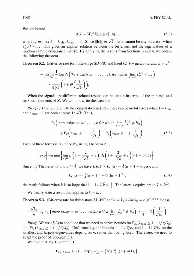
1068 A. FEY ET AL.
We can bound|((I − W )sZ)i | ≤ εs
k‖b‖2, (5.2)
where εk = max{1 − λmin, λmax − 1}. Since ‖b‖2 = √k, there cannot be any bit errors when
εsk
√k < 1. This gives an explicit relation between the bit errors and the eigenvalues of a
random sample covariance matrix. By applying the results from Sections 3 and 4, we obtainthe following theorem.
Theorem 5.2. (Bit-error rate for finite-stage SD-PIC and fixed k.) For all k such that k > 22s ,
−lim infn→∞
1
nlog Pk
(there exists m = 1, . . . , k for which lim
s→∞ b(s)m �= bm
)
≥ 1
4 s√
k
(1 + O
(1
s√
k
)).
When the signals are different, related results can be obtain in terms of the minimal andmaximal elements of Z. We will not write this case out.
Proof of Theorem 5.2. By the computation in (5.2), there can be no bit errors when 1−λminand λmax − 1 are both at most 1/
2s√
k. Thus,
Pk
(there exists m = 1, . . . , k for which lim
s→∞ b(s)m �= bm
)
≤ Pk
(λmin ≤ 1 − 1
2s√
k
)+ Pk
(λmax ≥ 1 + 1
2s√
k
). (5.3)
Each of these terms is bounded by, using Theorem 2.1,
exp
{−n min
{limε↓0
Ik
(1 − 2
2s√
k− ε
), Ik
(1 + 2
2s√
k+ ε
)}(1 + o(1))
}.
Since, by Theorem 4.1 and α ≥ 12 , we have Ik(α) ≥ I∞(α) = 1
2 (α − 1 − log α), and
I∞(α) = 14 (α − 1)2 + O(|α − 1|3), (5.4)
the result follows when k is so large that 1 − 1/2s√
k > 12 . The latter is equivalent to k > 22s .
We finally state a result that applies to k = kn.
Theorem 5.3. (Bit-error rate for finite-stage SD-PIC and k = kn.) For kn = o(ns/(s+1)/log n),
−s√
kn
nlog Pkn
(there exists m = 1, . . . , k for which lim
s→∞ b(s)m �= bm
)≥ 1
4+ O
(1
s√
kn
).
Proof. We use (5.3) to conclude that we need to derive bounds for Pkn(λmin ≤ 1 − 1/ 2s√
kn)
and Pkn(λmax ≥ 1 + 1/ 2s√
kn). Unfortunately, the bounds 1 − 1/ 2s√
kn and 1 + 1/ 2s√
kn on thesmallest and largest eigenvalues depend on n, rather than being fixed. Therefore, we need toadapt the proof of Theorem 3.1.
We note that, by Theorem 3.1,
Pkn(λmax ≥ 2) = exp{−( 1
2 − 12 log 2
)n(1 + o(1))
}.
Large deviations for eigenvalues of sample covariance matrices 1069
Then, we use (3.13) with �n = 2, and choose Rn such that
2
Rn
= o
(1
2s√
kn
),
so that Rn � 2s√
kn. Applying (3.12) and (3.9), we see that we need Rknn = exp{o(n/ s
√kn)}, so
that kn = o(ns/(s+1)/log n) is sufficient. Finally, by Theorem 4.1 and (5.4), we have
Ikn
(1 ± 1
2s√
kn
)≥ 1
4 s√
kn
(1 + O
(1
s√
kn
)).
This completes the proof.
We now discuss the above results. In [20], it was conjectured that, when s = 2, the rate ofa single bit error for a fixed user is asymptotic to 1/2
√k when k → ∞. See also [21]. We see
that we obtain a similar result, but our constant is 14 rather than the expected 1
2 . On the otherhand, our result is valid for all s ≥ 2.
Related results where obtained for a related model, hard-decision parallel interferencecancellation (HD-PIC), where bits are iteratively estimated by bits, i.e. the estimates are roundedto ±1. Thus, this scheme is not linear, as SD-PIC is. In [18] and [19], similar results to the abovewere obtained, and it was shown that the rate for a bit error for a given user is asymptotic to(s/8) s
√4/k when s is fixed and k → ∞. This result is similar in spirit to the one in Theorem 5.2.
The explanation of why the rate tends to 0 as 1/s√
k is much simpler for the case of SD-PIC,where the relation to eigenvalues is rather direct, compared to the explanation for HD-PIC,which is much more elaborate. It is interesting to see that both when s = ∞ and when s isfinite and k → ∞, the rates in the two systems are of the same order.
Interestingly, in [22], it was shown that, for s = 1 and kn = n/γ log n, with high probability,all bits are estimated correctly when γ < 2, while, with high probability, there is at least onebit error when γ > 2. Thus, kn = O(n/log n) is critical for the MF system, where we do notapply SD-PIC. For SD-PIC with an arbitrary number of stages of SD-PIC, we have no bit errorswith large probability for all kn = n/γ log n for all γ > 0, and we can even pick larger valuesof kn such that kn = o(n/log log n). Thus, SD-PIC is more efficient than MF, in the sense thatit allows more users to transmit without creating bit errors. Furthermore, in [22], the resultsproved in this paper are used for a further comparison between SD-PIC, HD-PIC, and MF.Unfortunately, when we apply only a finite number of stages of SD-PIC, we can allow only forkn = o(ns/(s+1)/log n) users. Similar results were obtained for HD-PIC when kn = o(n/log n).
We close this discussion on SD-PIC and HD-PIC by noting that, for k = βn, λmin convergesto (1 − √
β)2+, while the largest eigenvalue, λmax, converges to (1 + √β)2 (see [3], [4],
and [23]). This is explained in more detail in [9], and illustrates that SD-PIC has no bit errorswith probability converging to 1 whenever β < (
√2 − 1)2 ≈ 0.17 . . . . However, unlike the
case where kn = o(n/log log n), we do not obtain bounds on how the probability of a bit errortends to 0.
A further CDMA system is the decorrelator, which explicitly inverts the matrix W (withoutapproximating it by the partial sum
∑s−1ς=0(I − W )ς ). One way of doing so is to fix a large
value M and to compute
Z(s)M = M−1
s−1∑ς=0
(I − W
M
)ς
WZ
andb
(s)m,M = sgn(Z
(s)m,M).
1070 A. FEY ET AL.
This is a certain weighted SD-PIC scheme. This scheme will converge to b as s → ∞ wheneverλmin > 0 and λmax < M . By taking M such that I∞(M) ≥ log 2, and using Proposition 4.1,we obtain the following result.
Theorem 5.4. (Bit-error rate for optimal weighted SD-PIC.) For all k fixed, or for k = kn → ∞such that kn = o(n/log log n) and M such that I∞(M) ≥ log 2,
−1
nlog Pk(there exists m = 1, . . . , k for which b
(s)m,M �= bm) ≥ log 2. (5.5)
The above result can even be generalized to kn that grow arbitrarily fast with n, by takingM dependent on n. For example, when we take M > kn, λmax ≤ kn < M is guaranteed.
Further interesting problems arise when we allow the received signal to be noisy. In thiscase, the bit error can be caused either by the properties of the eigenvalues, as in the case whenthere is no noise, or by the noise. When there is noise, weighted SD-PIC for large M enhancesthe noise, which makes the problem significantly harder. See [13] for further details. A solutionto Conjecture 4.1 may prove to be useful in such an analysis.
Acknowledgements
The work of AF and RvdH was supported in part by NWO. The work of RvdH and MJKwas performed in part at Delft University of Technology.
References
[1] Bai, Z. D. and Silverstein, J. W. (1998). No eigenvalues outside the support of the limiting spectral distributionof large-dimensional sample covariance matrices. Ann. Prob. 26, 316–345.
[2] Bai, Z. D. and Silverstein, J. W. (2004). CLT for linear spectral statistics of large-dimensional samplecovariance matrices. Ann. Prob. 32, 553–605.
[3] Bai, Z. D. and Yin, Y. Q. (1993). Limit of the smallest eigenvalue of a large-dimensional sample covariancematrix. Ann. Prob. 21, 1275–1294.
[4] Bai, Z. D., Silverstein, J. W. and Yin, Y. Q. (1988). A note on the largest eigenvalue of a large-dimensionalsample covariance matrix. J. Multivariate Anal. 26, 166–168.
[5] Buehrer, R. M., Nicoloso, S. P. and Gollamudi, S. (1999). Linear versus non-linear interference cancellation.J. Commun. Networks 1, 118–133.
[6] Dembo, A. and Zeitouni, O. (1998). Large Deviations Techniques and Applications, 2nd edn. Springer, NewYork.
[7] Den Hollander, F. (2000). Large Deviations (Fields Inst. Monogr. 14). American Mathematical Society,Providence, RI.
[8] Fey-den Boer, A. C., van der Hofstad, R. and Klok, M. J. (2003). Linear interference cancellation inCDMA systems and large deviations of the correlation matrix eigenvalues. In Proc. Symp. IEEE Benelux ChapterCommum. Veh. Tech. (Eindhoven, 2003).
[9] Grant, A. and Schlegel, C. (2001). Convergence of linear interference cancellation multiuser receivers. IEEETrans. Commun. 49, 1824–1834.
[10] Guionnet, A. (2002). Large deviations asymptotics for spherical integrals. J. Funct. Anal. 188, 461–515.[11] Guo, D., Rasmussen, L. K., Tun, S. and Lim, T. J. (2000). A matrix-algebraic approach to linear parallel
interference cancellation in CDMA. IEEE Trans. Commun. 48, 152–161.[12] Hiai, F. and Petz, D. (1998). Eigenvalue density of the Wishart matrix and large deviations. Infin. Dimens.
Anal. Quantum Prob. 1, 633–646.[13] Klok, M. J. (2001). Performance analysis of advanced third generation receivers. Doctoral Thesis, Delft
University of Technology.[14] Marchenko, V. A. and Pastur, L. A. (1967). The distribution of eigenvalues in certain sets of random matrices.
Mat. Sb. 72, 507–536.[15] Olivieri, E. and Vares, M. E. (2005). Large Deviations and Metastability (Encyclopedia Math. Appl. 100).
Cambridge University Press.[16] Rasmussen, L. K. and Oppermann, I. J. (2003). Ping-pong effects in linear parallel interference cancellation
for CDMA. IEEE Trans. Wireless Commun. 2, 357–363.

Large deviations for eigenvalues of sample covariance matrices 1071
[17] Rogers, C. A. (1963). Covering a sphere with spheres. Mathematika 10, 157–164.[18] Van der Hofstad, R. and Klok, M. J. (2003). Performance of DS-CDMA systems with optimal hard-decision
parallel interference cancellation. IEEE Trans. Inf. Theory 25, 2918–2940.[19] Van der Hofstad, R. and Klok, M. J. (2004). Improving the performance of third-generation wireless
communication systems. Adv. Appl. Prob. 36, 1046–1084.[20] Van der Hofstad, R., Hooghiemstra, G. and Klok, M. J. (2002). Analytical methods for CDMA systems
with parallel interference cancellation: the large deviation approach. Wireless Personal Commun. 21, 289–307.[21] Van der Hofstad, R. Hooghiemstra, G. and Klok, M. J. (2002). Large deviations for code division multiple
access systems. SIAM J. Appl. Math. 62, 1044–1065.[22] Van der Hofstad, R., Löwe, M. and Vermet, F. (2006). The effect of system load on the existence of bit
errors in CDMA with and without parallel interference cancelation. IEEE Trans. Inf. Theory 52, 4733–4741.[23] Yin, Y. Q., Bai, Z. D. and Krishnaiah, P. R. (1988). On the limit of the largest eigenvalue of the large-
dimensional sample covariance matrix. Prob. Theory Relat. Fields 78, 509–521.