Large-eddy simulation of compressible flows using aspectral multi-domain method

K. Sengupta1, G. B. Jacobs2 and F. Mashayek1∗

1 Department of Mechanical and Industrial Engineering, University of Illinois at Chicago,842 W. Taylor, Chicago, IL 60607.

2 Department of Aerospace Engineering, San Diego State University,5500 Campanile Drive, San Diego, CA 92182

SUMMARY

This paper discusses the development of a high-order, multidomain based large-eddy simulation(LES) for compressible flows. The LES model equations are approximated on unstructured gridsof non-overlapping hexahedrals subdomains providing geometric flexibility. In each domain a high-order Chebyshev polynomial approximation represents the solution ensuring a highly accurateapproximation with little numerical dispersion and diffusion. The sub-grid scale stress in the filteredLES equations is modeled with a dynamic eddy viscosity model, while the heat flux is representedwith an eddy diffusivity model, employing a turbulent Prandtl number. The model constants areevaluated through a flexible dynamic procedure, that uses a high-order domain level filtering for thediscrete test filter. The LES methodology is tested in a decaying isotropic turbulence and channelflow. The LES method improves the resolution of the turbulence spectrum as compared to a directnumerical simulation with the same method at the same grid resolution. The averaged and secondorder statistics for LES computations are in close agreement with published results and resolveddirect numerical simulations. The high-order LES methodology requires fewer degrees of freedom ascompared to lower order LES methodologies to accurately resolve the turbulent flows.

key words: Large-eddy simulation; multidomain method; compressible flow; spectral element

filtering; isotropic turbulence; channel flow

1. INTRODUCTION

Large-eddy simulation has proven to be a viable technique for the computation of

unsteady turbulent flows with large coherent structures in real complex applications. At

moderate Reynolds numbers, LES is more economical and/or accurate than other established

∗Correspondence to: mashayek@uic.edu

2

computational techniques such as Direct Numerical Simulation (DNS) and Reynolds-Averaged

Navier-Stokes (RANS) methods. DNS solves the governing equations without any turbulence

modeling. Though it is accurate, DNS requires excessive computational cost to resolve the

increasing turbulence scale range with increasing geometric complexity and Reynolds number.

In RANS, on the other hand, all unsteady turbulence scales are modeled. While this reduces

computational cost and enables computation of most engineering applications, it also prevents

RANS from adequately capturing the true dynamics of the flow. LES bridges the gap between

DNS and RANS and efficiently computes unsteady turbulent flows in moderately complex

geometries at mid range Reynolds numbers found in many real applications. LES is based

on scale separation in turbulent flows. The large scales, which are anisotropic and sensitive

to boundary conditions are computed directly as in DNS, while the small scales that are

more isotropic and universal are modeled. The modeling of the small scales reduces the

computational cost, while the computation of the large scales provides detailed flow field

information.

Numerical schemes are crucially affecting the fidelity of large-eddy simulations. Numerical

errors in space and time can smear the solutions, overly dissipate turbulence, and so lead

to an inaccurate computation of the turbulent flow. Ghosal [1] performed an analysis of the

effect of numerical errors of a finite difference method on large-eddy simulation. He found

that for low order finite difference schemes, the truncation error may be larger than modeled

sub-grid stresses, unless the filter width is significantly larger than the grid size. Kravchenko

and Moin [2] later extended the analysis to include the role of aliasing errors. It was shown

that for low-order finite-differences, the high-wavenumber part of the energy spectrum is

heavily distorted by truncation errors and the contribution from the sub-grid model becomes

small. Inaddition, low-order schemes have large dispersion errors, which reduces the temporal

accuracy of unsteady (wave dominated) flow computations.

With a high-order scheme many of the numerical error related inaccuracies of lower-

order schemes can be reduced and fewer degrees of freedom are required for an accurate

solution. However, combining high-order accuracy with other desirable properties of a LES

method including geometric flexibility and conservation properties has proven challenging.

Conservative, low-order finite volume [3, 4] and finite element [5] methods have been developed

that allow for complex geometry computation, but the geometric flexibility of current high-

3

order LES, that mostly rely on spectral and compact finite difference methods [6], is limited.

Single domain spectral methods based on for example Fourier series approximations have

desirable high-wavenumber characteristics, but can only be used for rectangular geometries.

Compact finite difference methods are more versatile than the single domain spectral schemes.

However, the block Cartesian mesh requirement and overlapping stencil of compact difference

methods complicates both boundary condition implementation and an accurate, robust,

parallel implementation for complex geometries. Another drawback of the high accuracy of

both spectral and high-order finite difference methods is that aliasing errors affect the stability

of the methods. Aliasing errors can be reduced by a modified form of the non-linear advection

terms [7] or by using non-conservative form of the energy equation [8]. Unfortunately these

modifications do not guarantee robustness especially at high Mach numbers.

Spectral element methods [9, 10] are excellent candidates for LES, since they combine the

accuracy of single domain spectral schemes with the flexibility of finite element method. In

spectral elements the spatial resolution can be conveniently altered either by increasing the

number of elements (h-refinement) or by increasing the polynomial order within the elements

(p-refinement). In smooth solution spaces, the method provides asymptotically exponential rate

of spatial convergence with p-refinement. Low dispersion errors in these methods lead to high

temporal accuracy, making them suitable for wave dominated, unsteady problems. Moreover,

low degree of data connectivity between non-overlapping elements facilitates efficient boundary

condition implementation and parallel implementation.

Though spectral/hp element based DNS computations are well established, there have been

limited attempts to perform spectral element based LES. Spectral element filtering strategies

for LES was studied by Blackburn and Schmidt [11]. They investigated three different filtering

techniques within two-dimensional spectral elements for the simulation of incompressible

turbulent channel flow with a dynamic sub-grid model. Fischer and Mullen [12] introduced

a spectral element filtering technique to stabilize their direct numerical simulation. Levin et

al. [13] applied a two-step filtering procedure to control the growth of non-linear instabilities

in their eddy resolving spectral element ocean model. A combined spectral element-Fourier

method was used by Karamanos [14] for LES with an explicit sub-grid model. Karamanos and

Karniadakis [15] introduced spectral vanishing viscosity concept for large-eddy simulation.

The implementation was tested for turbulent channel flow using Fourier discretization in the

4

streamwise direction and spectral/hp quadrilateral elements in the cross flow and wall-normal

directions. These studies have focused on LES of incompressible flows. To the best of the

authors knowledge there has not been any published work on LES of compressible flows using

spectral element method.

In this paper, we develop a spectral/hp element large-eddy simulation technique for

compressible flows using a Chebyshev spectral multi-domain method [16, 17, 18]. The

method combines many features that are desirable in a numerical methodology for large-eddy

simulation of turbulent flows in complex geometries, including: a high-order approximation

within each sub-domain which restricts the numerical errors; complex geometries are easily

computed with the unstructured hexahedral grid; the method is robust; the flux based

methodology leads to a conservative scheme; and the non-overlapping elements yield perfect

parallelization implementation as well as easy boundary condition implementation. We model

the sub-grid scales using an eddy-viscosity model. A flexible dynamic procedure is employed

to evaluate the sub-grid model constants. The explicit filtering associated with the dynamic

procedure is accomplished through a sub-domain based high-order Lagrange-interpolant

projection procedure consistent with the high-order multidomain method. The characteristics

of the LES methodology are tested in a decaying isotropic turbulence and a turbulent channel

flow.

The paper is organized as follows. First, we describe the governing equations for compressible

flows and present the numerical method. Then, we discuss the LES formulation including the

filtered equations, sub-grid models and the dynamic procedure. Next, we test our methodology

in an isotropic turbulence and a turbulent channel flow. Conclusions and recommendations are

reserved for the final section.

2. GOVERNING EQUATIONS AND NUMERICAL FORMULATION

2.1. Compressible Navier-Stokes equations

The governing equations for the compressible and viscous fluid flow are the conservation

statements for mass, momentum and energy. They are presented in non-dimensional,

5

conservative form with Cartesian tensor notation,∂ρ

∂t+

∂(ρuj)∂xj

= 0, (1)

∂(ρui)∂t

+∂(ρuiuj + pδij)

∂xj=

∂σij

∂xj, (2)

∂(ρe)∂t

+∂[(ρe + p)uj ]

∂xj= − ∂qj

∂xj+

∂(σijui)∂xj

. (3)

The total energy, viscous stress tensor and heat flux vector are, respectively, given as,

ρe =p

γ − 1+

12ρukuk, (4)

σij =µ

Ref

(∂ui

∂xj+

∂uj

∂xi− 2

3∂uk

∂xkδij

), (5)

qj = − µ

(γ − 1)RefPrfM2f

∂T

∂xj. (6)

The reference Reynolds number Ref is based on the reference density ρ∗f , velocity Uf∗, length

Lf∗, and molecular viscosity µ∗f and is given by Ref = ρ∗f Uf

∗Lf∗/µ∗f . Prf = µ∗f Cp/k∗ is

the reference Prandtl number. The superscript ∗ denotes dimensional quantities. The above

equation set is closed by the equation of state,

p =ρT

γM2f

, (7)

where Mf is the reference Mach number, taken to be 1 in this work. The conservation equations

can be cast in the matrix form∂Q

∂t+

∂F ai

∂xi− ∂F v

i

∂xi= 0, (8)

where

Q =

ρ

ρu1

ρu2

ρu3

ρe

, (9)

F ai =

ρui

ρu1ui + pδi1

ρu2ui + pδi2

ρu3ui + pδi3

(ρe + p)ui

, (10)

6

F vi =

0

σi1

σi2

σi3

−qi + ukσik

. (11)

Here Q is the vector of the conserved variables, while F ai and F v

i are the advective and viscous

flux vectors respectively, in the xi direction.

2.2. Numerical methodology

This section briefly describes the staggered-grid Chebyshev multidomain method. For a more

complete description of the method see [16, 18]. In this method, the computational domain,

Ω, is divided into non-overlapping hexahedral sub-domains, Dk,

Ω =∑

Dk. (12)

The sub-domains are mapped onto a unit hexahedron Dk ↔ [0, 1] × [0, 1] × [0, 1] by an

isoparametric mapping [19]. Isoparametric mapping ensures that the spectral accuracy of the

scheme is not affected by the domain boundary approximation. The staggered grid method uses

two sets of grids, one for the solution (Chebyshev-Gauss grid) and one for computation of the

fluxes (Chebyshev-Gauss-Lobatto grids). In one space dimension the Gauss and Gauss-Lobatto

quadrature points are defined by,

Xj+1/2 =12

1− cos

[(2j + 1)π

2N

], j = 0, ....N − 1, (13)

and

Xj =12

1− cos

[πj

N

], j = 0, ....N, (14)

respectively, on the unit interval [0, 1]. The Gauss grid in three-dimensions, henceforth referred

to as the ggg grid, is the tensor product of the one-dimensional grid defined in Eq. (13). The

solution vector, Q, where the tilde denotes mapped space, is approximated on the ggg grid, as

Qggg

(X, Y, Z) =N−1∑

i=0

N−1∑

j=0

N−1∑

k=0

Qggg

i+1/2,j+1/2,k+1/2hi+1/2(X)hj+1/2(Y )hk+1/2(Z), (15)

7

where N − 1 is the approximation order. Here hi+1/2 ∈ P N−1 is the Lagrange interpolating

polynomial defined on the Gauss grid,

hi+1/2(ξ) =N−1∏

m=0,m 6=i

(ξ −Xm+1/2

Xi+1/2 −Xm+1/2

). (16)

The fluxes in each direction F i are defined on the Gauss-Lobatto grids, shown in figure 1.

The x-direction flux (F 1) is evaluated at the Lobatto-Gauss-Gauss grid (lgg) denoted by open

squares, (Xi, Yj+1/2, Zk+1/2), i = 0, 1 · · ·N , j, k = 0, 1 · · ·N−1, the y-direction flux (F 2) at the

Gauss-Lobatto-Gauss grid (glg) denoted by open circles, (Xi+1/2, Yj , Zk+1/2), j = 0, 1 · · ·N ,

i, k = 0, 1 · · ·N−1 and the z-direction flux (F 3) at the Gauss-Gauss-Lobatto grid (ggl) denoted

by closed squares, (Xi+1/2, Yj+1/2, Zk), k = 0, 1 · · ·N , i, j = 0, 1 · · ·N −1. The flux vectors are

computed by reconstructing the solution at the Lobatto points through interpolations using

polynomials of the type in Eq. (15). The interpolation operation is given as,

Qlgg(Xi, Yj+1/2, Zk+1/2) =N−1∑m=0

N−1∑n=0

N−1∑p=0

Qggg

m+1/2,n+1/2,p+1/2

Jm+1/2,n+1/2,p+1/2hm+1/2(Xi)× (17)

hn+1/2(Yj+1/2)hp+1/2(Zk+1/2),

in the X-direction, which reduces to a one-dimensional operation,

Qlgg(Xi, Yj+1/2, Zk+1/2) =N−1∑m=0

Qggg

m+1/2,j+1/2,k+1/2

Jm+1/2,j+1/2,k+1/2hm+1/2(Xi), (18)

due to the cardinal property of the Lagrange interpolating polynomial. Similarly for the Y and

Z directions the interpolants are given by,

Qglg(Xi+1/2, Yj , Zk+1/2) =N−1∑n=0

Qggg

i+1/2,n+1/2,k+1/2

Ji+1/2,n+1/2,k+1/2hn+1/2(Yj), (19)

Qggl(Xi+1/2, Yj+1/2, Zk) =N−1∑p=0

Qggg

i+1/2,j+1/2,p+1/2

Ji+1/2,j+1/2,p+1/2hp+1/2(Zk), (20)

where, J is the Jacobian of transformation from the physical space to the mapped space. Once

the solution values are interpolated to the Lobatto grid the advective fluxes are computed.

The interface points will have different flux values due to discontinuity of solution values

at the sub-domain boundaries. The patching of the advective fluxes is described later. The

viscous fluxes are computed in two steps. The solution interpolant at the Lobatto grids must

be continuous for an unique first derivative at the subdomain interfaces. This is ensured by

8

a Dirichlet patching, or averaging of the solution on both sides of the interface. After the

Lobatto interpolants for the solution values are patched, their derivatives are computed at the

Gauss points. The gradients are then interpolated back to Lobatto points. The viscous fluxes

are computed using the functional relations (5) and (6). The interface condition for viscous

fluxes and any Neumann boundary condition are applied at this point. Finally, the total flux

is obtained by adding the inviscid and viscous parts. Once the total fluxes are computed at

the lgg, glg and ggl points, the flux interpolants are constructed as,

F1(X, Y, Z) =N∑

m=0

N−1∑n=0

N−1∑p=0

F1m,n+1/2,p+1/2lm(X)hn+1/2(Y )hp+1/2(Z), (21)

F2(X, Y, Z) =N−1∑m=0

N∑n=0

N−1∑p=0

F2m+1/2,n,p+1/2hm+1/2(X)ln(Y )hp+1/2(Z), (22)

F3(X, Y, Z) =N−1∑m=0

N−1∑n=0

N∑p=0

F3m+1/2,n+1/2,phm+1/2(X)hn+1/2(Y )lp(Z). (23)

These fluxes are differentiated and evaluated at the Gauss-Gauss-Gauss grid, to give pointwise

derivatives,

∂F1(Xi+1/2, Yj+1/2, Zk+1/2)∂X

=N∑

m=0

F1(Xm, Yj+1/2, Zk+1/2)∂lm(Xi+1/2)

∂X(24)

∂F2(Xi+1/2, Yj+1/2, Zk+1/2)∂Y

=N∑

n=0

F2(Xi+1/2, Yn, Zk+1/2)∂ln(Yj+1/2)

∂Y(25)

∂F3(Xi+1/2, Yj+1/2, Zk+1/2)∂Z

=N∑

p=0

F3(Xi+1/2, Yj+1/2, Zp)∂lp(Zk+1/2)

∂Z. (26)

Finally the semi-discrete equation for the solution unknowns at the Gauss-Gauss-Gauss grid

is given by, [dQ

dt

]

i+1/2,j+1/2,k+1/2

+

[∂F i

∂Xi

]

i+1/2,j+1/2,k+1/2

= 0, (27)

which is advanced in time using a 4th-order low storage Runge-Kutta scheme.

2.3. Interface and boundary treatment

Interpolation of the solution by Eqs. (18)-(20) leads to different solution values at the

sub-domain interface points, one from each of the contributing sub-domains. The solution

9

is therefore discontinuous. The coupling between sub-domains is enforced by a continuous

advective and viscous fluxes at the interface points. Enforcing flux continuity yields a

conservative method. The inviscid fluxes are computed using an approximate Riemann solver.

Formally, given the two solution states Qk−1N and Qk

0 (the superscript denotes the sub-domain

number and the subscript denotes the node number within a sub-domain), the flux in each

spatial direction, with the assumption that waves are normal to the interface, can be written

as,

Γa(Qk−1N , Qk

0) =12

[F a(Qk−1

N ) + F a(Qk0)

]− 1

2R|λ|R−1(Qk

0 −Qk−1N ), (28)

where Fa is the vector of advective fluxes. R is the matrix of the right eigenvectors of the

Jacobian of Fa, computed using Roe-average of Qk−1N and Qk

0 . For imposing inviscid boundary

conditions, the physical boundary can be viewed as an interface between the external state

and the computational domain. The Riemann solver is applied between the external specified

flow solution and internal solution vector.

The viscous fluxes are determined as outlined in the previous sub-section. Continuity of

the viscous fluxes is established by averaging the viscous flux vector from both sides of the

interface

Γv,k0 = Γv,k−1

N =12(F v,k

0 + F v,k−1N ). (29)

The Neumann boundary conditions are imposed at the boundary points at this stage.

3. LES FORMULATION

3.1. Filtered Navier-Stokes equations

The LES method presented here solves the filtered Navier-Stokes equations. By applying a

spatial low-pass (in frequency domain) convolution filter to the Navier-Stokes equations, the

turbulence scales are separated. The filter in physical space is represented by the following

convolution product,

f(x, t) =∫

Ω

f(x′, t)G(x− x

′)dx

′, (30)

10

where G is the filter kernel and Ω represents the flow domain. We apply the Favre, density

weighted filtering operation, typical for LES of compressible turbulence

f =ρf

ρ, (31)

where overbar denotes the filtering operation.

Applying this filter yields the following filtered conservation equations,

∂ρ

∂t+

∂(ρuj)∂xj

= 0, (32)

∂(ρui)∂t

+∂(ρuiuj + pδij)

∂xj=

∂σij

∂xj− ∂τ sgs

ij

∂xj+

∂(σij − σij)∂xj

, (33)

∂(ρe)∂t

+∂[(ρe + p)uj ]

∂xj= − ∂qj

∂xj+

∂(σij ui)∂xj

− 1(γ − 1)M2

f

∂qsgsj

∂xj+

∂(qj − qj)∂xj

+ (34)

∂(uj [σjk − σjk])∂xk

+12

∂

∂xjρ(ukukuj − ukukuj − τsgs

kk uj).

The filtering leads to several terms in Eqs. (33) and (34) that require closure. τsgsij is the

sub-grid scale stress tensor and qsgsj is the sub-grid turbulent heat flux. The sub-grid terms

physically represent the effect of the unresolved (sub-grid) scales on the resolved scales. The

second unclosed term in the filtered momentum equation is (σij−σij), which results from Favre

filtering of the viscous stresses. The filtered energy equation has three more unclosed terms

in addition to the sub-grid heat flux: the term ∂(qj−eqj)

∂xjwhich results from Favre filtering of

the diffusive heat flux; the term ∂(uj [σjk−eσjk])∂xk

which is analogous to the sub-grid scale viscous

dissipation; and finally the divergence of turbulent diffusion, 12

∂∂xj

ρ(ukukuj−ukukuj−τsgskk uj).

The modeling of the unclosed terms is discussed in Section 3.2.

3.2. Sub-grid scale model

The unclosed terms in the filtered equations require modeling. We first consider the modeling

of the unclosed terms in the momentum equation (Eq. (33)). The term (σij − σij) is neglected

following [20, 21]. The sub-grid term τsgsij = ρ(uiuj − uiuj) is modeled using the modification

of the Germano model [22] for compressible flows (given by Moin et al. [8]). The expression

for τsgsij is accordingly given as

τsgsij = −2Cs42

ρ|S|(

Sij − 13Smmδij

)+

13τsgskk δij . (35)

11

The trace of the sub-grid stress tensor τsgskk cannot be included in the modified pressure in

compressible flow, and thus has to be modeled separately. Different models of τsgskk have been

proposed (see [23, 24]). However, the study by Squires [25] demonstrated that there is no

difference in the LES results of compressible isotropic turbulence at low Mach number when

τsgskk is neglected. Vreman et al. [26] confirmed the above findings with their simulation of 3D

compressible mixing layers at a mean convective Mach number of 0.2. In their a priori test,

the SGS model that neglects τsgskk was found to be in better agreement with DNS results.

Moreover, simulations conducted with a dynamic model for τsgskk were often unstable for the

cases studied by Vreman et al. [26]. So, in LES of low Mach number flow, neglecting the trace

of sub-grid stress tensor will not introduce large errors. We will therefore neglect the term

here. The details of the dynamic procedure to obtain the estimate for Cs42are provided in

Section 3.3.

The sub-grid term

qsgsj = ρ

(T uj − T uj

)(36)

is described according to the derivation in [6] and is modeled using the eddy-viscosity

hypothesis and a turbulent Prandtl number. The modeled expression is,

qsgsj =

ρCs42|S|Prt

∂T

∂xj. (37)

The turbulent Prandtl number Prt is evaluated using the dynamic procedure (see Section 3.3).

A priori analysis of the magnitude of various terms in the filtered energy equation by Vreman

et al. [20] has shown that the fourth and fifth terms on the right-hand side of Eq. (34) are

small compared to the sub-grid heat flux vector and can be neglected, especially at low and

moderate Mach numbers. Finally, the last term in the filtered energy equation (Eq. (34)) is

similar to turbulent diffusion of sub-grid scale kinetic energy. The contribution of this term is

again small compared to other sub-grid terms (see [6]), although there has been some attempts

to model it (e.g. Okong’o et al. [27]). We neglected the term here.

3.3. Dynamic procedure

We employ a dynamic procedure to evaluate the constants in the modeled sub-grid terms.

The dynamic model [22] is based on self-similarity of the inertial range of the turbulence

12

energy spectrum at different length scales. Therefore, the same functional form for the sub-

grid quantities can be assumed at the grid length scale 4, representative of the computational

mesh, and at a larger test filter length scale 4. The application of the test filter to the grid

filtered Navier-Stokes equation (Eq. (33)) leads to a residual stress at the test filter level,

Tij = ρuiuj − ρuiρuj

ρ. (38)

Similarly, applying the test filter to the residual stresses at the grid filter level (τsgsij ) gives,

τsgsij = ρuiuj − ρuiρuj

ρ. (39)

The difference between Eqs. (38) and (39) leads to the Germano’s identity,

Lij = Tij − τsgsij = ρuiuj − ρuiρuj

ρ. (40)

Assuming that the same functional form (Smagorinsky model) could be used for the residual

stresses at both levels, we have the modeled forms as,

Tij = −2Cs42ρ|S|(

Sij − 1

3Smmδij

)+

13Tkkδij , (41)

τsgsij = −2Cs42

ρ|S|(

Sij − 13Smmδij

)+

13τsgskk δij . (42)

Substituting the above two expressions into Eq. (40) we obtain the modeled expression for Lij ,

Lmodij = Cs42

Mij − 13τ sgskk δij +

13Tkkδij . (43)

where Mij is defined as,

Mij = 2

ρ|S|(

Sij − 13Smmδij

)− 2

42

42 ρ|S|(

Sij − 1

3Smmδij

), (44)

where typicallyb44 = 2 is assumed. Here, we neglect both τsgs

kk and Tkk. Finally, using Lily’s

[28] least square minimization procedure we obtain,

Cs42=

LijMij

MklMkl, (45)

where Lij is explicitly given by Eq. (40). This procedure gives a local time-dependent estimate

of Cs42, which is updated at each time iteration. It is worthwhile to note that the above

procedure computes the Smagorinsky length scale Cs42directly without the need to specify

13

the grid filter width 4. This is advantageous in the current context considering that for

unstructured hexahedral grid it is difficult to provide a general expression for the filter width

4.

Since the solution, Q, is discontinuous, the value of Cs42is also discontinuous across the

sub-domains. The sub-grid length scale is used to evaluate the sub-grid momentum flux (Eq.

(35)), on which we impose continuity by averaging neighboring flux vectors. This is consistent

with the flux continuity of the multidomain method.

The turbulent Prandtl number (Eq. (37)) is evaluated using a dynamic procedure similar to

the one described above. A heat flux vector at the test filter level is defined analogous to the

heat flux at the grid filter level (Eq. (36)),

Qj = ρujT − 1ρρT ρuj . (46)

Applying the test filter on the sub-grid heat flux (Eq. (36)) and subtracting the resulting

expression from the test filter heat flux gives an expression analogous to the Germano’s identity

(Eq. (40)),

Kj = Qj − qsgsj = ρT uj −

ρT ρuj

ρ . (47)

The same eddy diffusivity model is used for the heat flux at the test filter level,

Qj =−Csρ42|S|

Prt

∂T

∂xj. (48)

Therefore, substituting Eqs. (37) and (48) into Eq. (47), the modeled form for Kj is obtained

as,

Kmodj =

Cs42

Prt

ρ|S| ∂T

∂xj− ˆρ

42

42 |S| ∂

T

∂xj

. (49)

Finally, following the procedure for computing the sub-grid viscosity, a least square

minimization technique is used for evaluating the sub-grid Prandtl number,

Prt =2NiNi

KjNj(Cs42

), (50)

where Ni is given by,

Ni =

ρ|S| ∂T

∂xi− ˆρ4|S| ∂

T

∂xi, (51)

assumingb44 = 2 and Cs42

is given by Eq. (45).

14

3.4. Element level filtering

The dynamic procedure requires the definition of an explicit, low pass filter for the test filtering

operation. Spectral filtering can be constructed using either discrete polynomial transform

(DPT) or interpolant-projection (see [11]) over each element. DPT filtering can be conveniently

applied for methods with modal basis. For methods with nodal basis, the solution has to be

first transformed to modal basis before the DPT filter can be applied. Projection filtering on

the other hand can be constructed directly on the nodal basis. Since it does not require an

extra transformation, interpolant-projection filtering is more efficient than DPT for methods

with nodal basis. Therefore, for our nodal basis we use an interpolant-projection filter.

In the interpolant-projection filtering procedure, the filtered variable of degree N is obtained

by projecting the variable back and forth to a lower order approximation of degree M defined

on a subset of the original nodal values. As a first step the original function is interpolated

from a polynomial degree, N , to a polynomial of lower degree, M ,

Q′(xi) =

N∑

j=0

Lj(xi)Q(xj), (52)

where xi, xj are the nodes corresponding to PM and PN , respectively. Lj ∈ PN is the Lagrange

interpolating polynomial. The above operation can be cast in terms of matrix-vector product,

Q′i = Iint

ij Qj , (53)

where

Iintij =

N∏

k=0,k 6=j

xi − xk

xj − xk, i = 0, · · · , M, j = 0, · · · , N. (54)

In the second step the function Q′(x) is projected back to the polynomial space N giving the

filtered function,

Qfilt(xe) =M∑

f=0

Lf (xe)Q′(xf ). (55)

Again, the above can be cast in matrix-vector form,

Qfilte = Ipro

ef Q′f , (56)

with

Iproef =

M∏

k=0,k 6=f

xe − xk

xf − xk, e = 0, · · · , N, f = 0, · · · ,M. (57)

15

In the staggered grid method, this interpolation-projection operation could be applied to

both the nodal sets (Gauss-Gauss and Gauss-Lobatto nodes). We apply the filter on the

Gauss-Lobatto basis since it preserves the end values of the original function and ensures C0

continuity.

4. TESTING THE LARGE-EDDY SIMULATION METHOD

We test the performance of the staggered grid, multidomain large-eddy simulation method

for two different classes of turbulent flows. The first case study is on an isotropic decaying

turbulence, and enables a first order investigation of the characteristics of the LES method,

since the flow doesn’t involve turbulence shear production and specification of boundary

conditions. Many sub-grid models have been calibrated with this flow (e.g. [22, 29]). Then,

we perform a more complex test by simulating a plane, parallel channel flow at two different

Reynolds numbers, that does involve boundary condition specification and shear production.

4.1. Decaying isotropic turbulence

Computation of the decaying isotropic turbulence is performed within a periodic box of size

2π. An initial correlated turbulence flow field is specified according to the procedure outlined

by Rogallo [30] using a specified energy spectra. We take an initial energy spectrum that

was modeled in Blaisdell et al. [31]. We refer to this spectrum and case as BMR93. The

spectra are purely solenoidal (divergence free) and there is no fluctuation in the thermodynamic

variables. The spectra are top hat and have non-zero contributions in the wavenumber range

of 8 ≤ k ≤ 16. The initial flow field for velocities (u, v, w), density (ρ) and temperature (T) are

obtained on a uniform grid from the Fourier coefficients using a fast Fourier transform. The

resultant flow field is correlated according to the top hat spectra. Finally, the initial flow field

on the Chebyshev-Gauss points is obtained by interpolating from the Fourier grid using an

eighth-order Lagrangian interpolation. The interpolation was shown to be adequately accurate

even for low polynomial orders in [16]. The initial root mean square (rms) Mach number is 0.3

with a peak Reλ ≈ 40.

Resolution and spectra

We start by establishing resolution requirements for a resolved LES and the effect of

16

resolution on the accurate representation of the spectrum. To this end, we computed several

cases with different h and p resolutions that are summarized in table I. The number of sub-

domains in x, y, and z direction is given by hx, hy and hz, while p represents the order of

polynomial in each sub-domain. LES-BASE is the base case with six domains in each directions

and p=8. LES-RFNDp and LES-RFNDh have a finer resolution of p=10 and h=7, respectively.

The DNS-RES and DNS-URES refer to a resolved and unresolved DNS without filtering.

The total energy spectra in figure 2 show that the resolved DNS (DNS-RES) is in good

agreement with previously published BMR93 data. The sharp, matching drop-off in the spectra

indicates that the DNS is resolved. The BMR93 case was computed with a Fourier-spectral

method with 963 grid points. DNS-RES uses comparable amount of degrees of freedom with

h=6 domains in each direction and p=15, yielding h ∗ (p + 2) = 102 Lobatto points in each

direction, to resolve the flow. This is consistent with the validation study in [16].

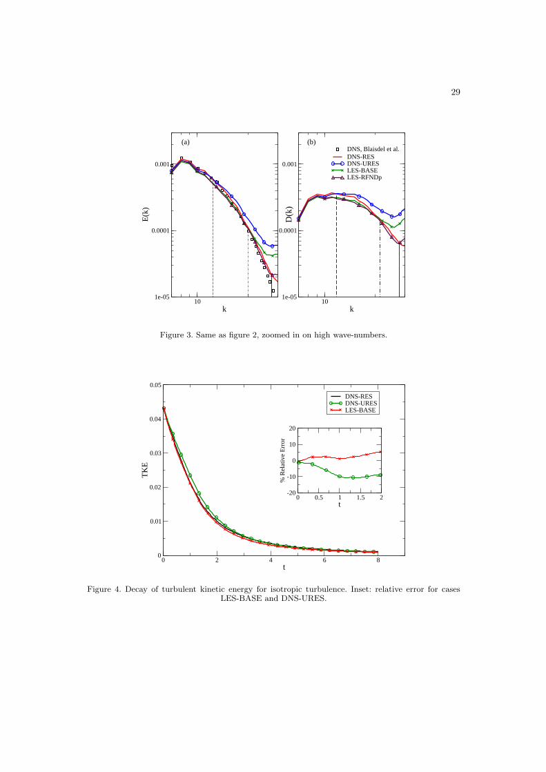
Comparison of the energy and dissipation spectra between DNS-URES, LES-BASE and

the resolved DNS-RES (figure 2), reveals that LES is clearly capturing the drop-off in the

spectra better than the under-resolved DNS. A zoom-in on the high-frequency part (k ≥ 7)

of the spectrum in figure 3 underscores the improved capturing. LES-BASE resolves the flow

upto k ≈ 20 while the increase of the spectrum for k ≥ 12 of the coarse DNS indicates an

inaccurate solution. The dashed-dashed line in the figure highlights the point upto which there

is agreement between the BMR93 spectra and DNS-URES, while the dashed-dot line shows the

same for LES-BASE. Clearly the sub-grid model in LES is correctly modeling the dissipative

effect of the small scale on the turbulence, that leads to the steep drop-off of the spectrum

at high wavenumbers. While in a resolved DNS these small scales are accurately captured,

in the under-resolved DNS insufficient resolution is unable to accurately compute the high-

frequency spectrum. Instead, the numerical errors determine the behavior at the small scale.

In a numerical method with very small dissipation like the multi-domain spectral method, the

numerical errors are not dissipated like in dissipative method (e.g. upwind schemes). Rather,

the numerical errors pile up at high wavenumbers, as seen in the spectra. In LES, the scales

upto k = 20 are numerically resolved. At k ≥ 12 the LES sub-grid model accurately models

the dissipative term to the filtered equations.

Comparison of the turbulence kinetic energy (tke) decay rate for DNS-RES, DNS-URES

and LES-BASE in figure 4, confirms the improved dissipation modeling. At t = 2, 75% of

17

the initial energy has decayed. The decay rate determined with LES is in closer agreement

with DNS-RES than the rate determined with DNS-URES. DNS-URES under-predicts the

decay rate. The additional dissipation provided by the sub-grid model in LES increases the

turbulence dissipation and improves comparison with DNS-RES. In the inset of figure 4 we

plot the percentage relative error, defined as (tkeDNS−RES − tke)/tkeDNS−RES × 100, for LES-

BASE and DNS-URES. On average, the magnitude of error for the coarse DNS is twice of the

LES case.

We assess the resolution requirement for LES with multidomain Chebyshev method from

the cutoff wavenumber (kc = 20). The total number of Lobatto points in each direction is 60

(6 sub-domains times 10 Lobatto points). This implies that in order to resolve the spectrum

till k = 20, 3 points are needed per wavelength. The value is further confirmed by the refined

LES case (LES-RFNDp), where the total number of Lobatto points is 72 (6 sub-domains times

12 Lobatto points) and the flow is resolved upto k = 27 (the cut-off is marked by solid line).

Therefore, again 72/27 ≈ 3 points are required per wavelength. This resolution is consistent

with the requirements reported in [16].

Dilatational and thermodynamic field

Decomposition of the velocity spectrum into solenoidal (figure 5(a)) and dilatational

spectrum (figure 5(b)), shows that the dilatational spectrum is two orders of magnitude less

than the solenoidal spectrum, which is in agreement with BMR93. The solenoidal velocity

is associated with vorticity [32]. The vortical mode can generate both larger length scales,

through vortex merging and smaller scales, through vortex stretching. Therefore, the initial

tophat solenoidal spectrum smoothes out at both low and high wavenumbers in time.

The dilatational velocity is associated with the acoustic and entropy mode [32]. In the

acoustic mode small length scales are generated through non-linear steepening of pressure

waves, but there is no direct mechanism for generation of larger length scales like in

the solenoidal mode. Since the simulation is started with zero fluctuations in dilatational

velocity and thermodynamic fields, the acoustic fluctuations were created through non-linear

production from the solenoidal velocity field. For small turbulent Mach numbers the length

scale of the acoustic fluctuations generated from the vorticity fluctuations is much larger than

the length scale of vortical turbulence [16, 31]. In time the acoustic length scales grow to

become comparable to the size of the simulation box and hence cannot be resolved. As a result

18

the dilatational velocity spectra has a very flat character at low wavenumbers. Case DNS-

RES shows good agreement for the dilatational spectrum upto k = 15, but the sharp drop-off

at high wavenumbers as in BMR93 is not observed. Since the dilatational spectrum is two

orders of magnitude less than the solenoidal spectrum, a much higher resolution is required

to capture the drop-off. This is evident from figure 5(b), where the spectrum for a DNS

case with p = 20 and h = 6 shows better agreement with BMR93. However, the dilatational

spectrum has very small contribution to the total spectrum and therefore the case DNS-RES,

which accurately resolves the solenoidal spectrum is considered as the resolved DNS. The

dilatational spectra for case LES-BASE is closer to BMR93 than DNS-URES (coarse DNS).

The normalized fluctuations of pressure and density are shown in figure 6 for cases DNS-RES,

DNS-URES and LES-BASE. Both pressure and density fluctuations initially grows with time

as energy is drained from the velocity field. After attaining peaks, which are approximately

same for both the quantities, they start decaying. The figure shows that LES-BASE predicts

a more accurate decay than DNS-URES.

Test filter effect

The Lagrange interpolant-projection filtering requires two sets of Lobatto grids (section

3.4). The polynomial space of degree N is fixed by the polynomial approximation used within

each subdomain for the flow computation , i.e. N = 10 when p = N− 2 = 8. On the other

hand, the size of the lower-degree grid of order, M, used for the interpolation can be varied

independently and determines the strength of the test filter. With decreasing M, the strength

and consequently the effect of the filter is larger. To investigate how the degree M of the

lower-order grid affects the flow, LES results based on two test filters are compared, listed as

LES-BASE and LES-FILT in table I. The lower-order grid for the test filter of LES-BASE is

of degree M = (N + 1)/2, while the test filter in LES-FILT is of degree M = N− 2.

The decay of turbulence kinetic energy for the two LES cases are compared with DNS-RES

in figure 7. The percentage relative errors are shown in the inset of the figure. LES-BASE has

a lower error for t < 1, while for t > 1 the error magnitude is lower for LES-FILT. For both

cases the predictions are within 5% of the reference case, indicating that the choice of the

filter strength has small influence on the decay of turbulent kinetic energy, since the sub-grid

viscosities are nearly equal in both cases. Decays of normalized fluctuations of pressure and

density (shown in figure 8), however, show considerable differences. For both quantities, the

19

decay rate for LES-FILT has larger deviation from the reference DNS case (DNS-RES), as

compared to LES-BASE. This indicates that the modeled sub-grid quantities in LES-BASE is

able to reproduce the cascade of energy in acoustic and entropy mode accurately. Therefore,

we conclude that when the effect of the test filter is larger, more small scale acoustic waves

are modeled.

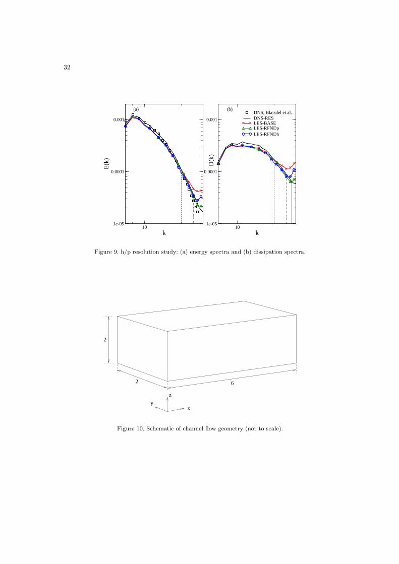
h/p resolution study

One of the distinguishing aspects of spectral/hp element methods is the feature of controlling

the spatial resolution at two different levels. The resolution can be altered either by changing

the number of sub-domains (h-refinement) or by changing the order of the polynomial within

each sub-domain (p-refinement).

Here, we study the effect of independently changing the h and p resolutions on the LES

results. Cases LES-BASE and LES-RFNDp have the same h-grid but different polynomial

orders, while cases LES-BASE and LES-RFNDh have the same polynomial order but different

h-grids. The total number of Lobatto points for cases LES-RFNDp and LES-RFNDh are 72

and 70, respectively, which is comparable. The total energy spectra for cases LES-BASE,

LES-RFNDp and LES-RFNDh is shown in figure 9. As the polynomial order is increased from

p = 8 (LES-BASE) to p = 10 (LES-RFNDp), the maximum resolved wavenumber increases

from k = 20 (the cut-off is marked by dashed-dashed line) to k = 27 (the cut-off is marked

by solid line). Whereas, increasing the number of sub-domains in each direction from h = 6

(LES-BASE) to h = 7 (LES-RFNDh), the maximum resolved wavenumber increases to k = 25

(the cut-off is marked by dashed-dot line). This indicates that p-refinement resolves the flow

better than h-refinement, which is consistent with the h/p spectral convergence [9].

4.2. Turbulent channel flow

Next, the LES methodology is tested for a three-dimensional, subsonic, plane, parallel channel

flow. Presence of the wall significantly increases the complexity of the flow, the analysis and

the LES implementation as compared to the isotropic turbulence case. Traditionally, the near

wall region in LES of wall bounded flows is either resolved with a fine mesh like in DNS, or

modeled [33]. Moin and Kim [34] performed LES of incompressible channel flow, with a Fourier

spectral-finite difference scheme using a non-dynamic eddy viscosity model. Application of the

dynamic Smagorinsky model to incompressible channel flow at high Reynolds numbers was

20

studied by Piomelli [35], where a Fourier-Chebyshev pseudospectral collocation scheme was

used. Wang and Pletcher [36] performed LES of low speed flows with significant heat transfer

at the wall, using a low Mach number algorithm coupled to a dynamic eddy viscosity model.

LES of compressible channel flow in both subsonic and supersonic regimes, at a bulk Reynolds

number of 3000 was performed by Lenormand et al. [37]. They used fourth and second order

finite difference to discretize the convective and diffusive terms, respectively. The subgrid scales

were represented through Smagorinsky and scale similarity models. Channel flow was also used

for validating LES methodologies with finite element (e.g. [5]) and spectral element (e.g. [11])

methods. In [5] it was shown that the finite element method gave better prediction of the

normal Reynolds stresses over a second order central difference scheme. In their validation

study, Blackburn and Schmidt [11] found that test filtering in Legendre basis gave best result

for the mean velocity profile, while the projection filter provided best agreement with DNS for

both normal and shear stress.

Computational model

A schematic of the computational domain is shown in figure 10. The domain extents are

Lx = 6, Ly = 2, Lz = 2 in the streamwise, spanwise and wall normal directions, respectively.

Periodic boundary conditions are employed in the streamwise and spanwise directions, while

the conservative isothermal wall boundary condition of Jacobs et al. [38] is used for the bottom

and top wall. The flow is simulated at bulk Reynolds number of Ref = 3000 and Ref = 10, 000,

based on channel half width and bulk velocity. The corresponding friction Reynolds numbers

were Reτ ≈180 and Reτ ≈570, respectively. The Mach number is taken to be Ma = 0.4 based on

bulk velocity and wall temperature (Twall). Following Lenormand et al. [37], a time dependent

forcing term is included in the streamwise momentum equation in order to drive the flow.

The velocity field is initialized with the laminar parabolic profile for u with a small random

disturbance superimposed on it,

u(z) = −6[(z

2

)2

− z

2

](1 + ε), v = 0, w = 0, (58)

where ε is a 10% random disturbance. The temperature is initially set to laminar Poiseuille

profile,

T (z) = Twall +

3(γ − 1)4Pr

[1− (z − 1)4

]. (59)

Here Twall = 6.25 is the wall temperature and Pr = 0.72 is the Prandtl number. The density is

21

initially set as constant. The initial pressure is calculated from the constant density, the initial

temperature and the ideal gas law. Previous studies [16, 39] have shown that at Ma = 0.4,

plane parallel channel flow is pseudo-incompressible. Therefore, our simulation results are

compared with incompressible DNS study of Moser et al. [40] and experimental measurements

of Niedershulte et al. [41].

Low-Reynolds-number simulation

The first test case is for Re = 3000. This is close to the lowest Reynolds number at which

a fully developed turbulent channel flow can be sustained without relaminarization. The

computational domain (figure 10) is decomposed with 10 sub-domains in the streamwise (x)

and spanwise (y) directions, while 16 sub-domains are taken in the wall normal (z) direction.

The sub-domains in the wall direction are stretched out towards the center of the channel with

a cosine distribution. The polynomial order within each sub-domain is taken as p = 6. The

total number of Lobatto points for the above h/p grid is 819,200. The subgrid constant Cs42

and Prt are obtained by averaging right-hand side of Eqs. (45) and (50) along homogenous

(x-y) planes within each sub-domain,

Cs42=

⟨LijMij

MklMkl

⟩, P rt =

⟨2NiNi

KjNj

⟩ (Cs42

). (60)

where 〈〉 indicates averaging. This averaging technique was proposed by Zhao and Voke [42],

and was shown to be more stable and give better agreement with the asymptotic behavior of

turbulent length scales near the wall as compared to the Germano-Lily averaging approach

[22]. The sub-grid viscosity is computed once in every time step.

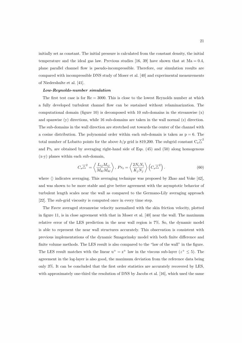
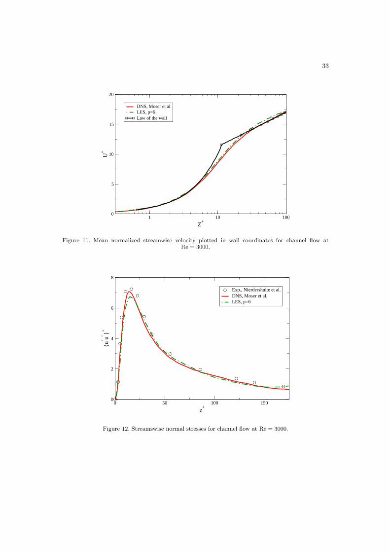
The Favre averaged streamwise velocity normalized with the skin friction velocity, plotted

in figure 11, is in close agreement with that in Moser et al. [40] near the wall. The maximum

relative error of the LES prediction in the near wall region is 7%. So, the dynamic model

is able to represent the near wall structures accurately. This observation is consistent with

previous implementations of the dynamic Smagorinsky model with both finite difference and

finite volume methods. The LES result is also compared to the “law of the wall” in the figure.

The LES result matches with the linear u+ = z+ law in the viscous sub-layer (z+ ≤ 5). The

agreement in the log-layer is also good, the maximum deviation from the reference data being

only 3%. It can be concluded that the first order statistics are accurately recovered by LES,

with approximately one-third the resolution of DNS by Jacobs et al. [16], which used the same

22

Chebyshev spectral multidomain method, and Moser et al. [40] who used a pseudo-spectral

code. The gain in computational time is slightly offset by the computational overhead of the

sub-grid model. The cost of LES was 1.44 times that of the simulation without the sub-grid

model on the same grid.

In figure 12, the resolved-scale Favre-fluctuating streamwise turbulent stress computed with

LES, is compared to the DNS and the experiment. The results are normalized with u2τ and

plotted in wall coordinates. It is noted that although the usual practice in a posteriori testing

is to compare the resolved-scale Reynolds stresses from LES directly with unfiltered DNS or

experiment, the two quantities are not equivalent and therefore are not expected to match

exactly. The location for the peak streamwise fluctuation is accurately represented by LES,

although there is a 4% under-prediction in the magnitude of the peak. Except for the peak

value, the resolved-scale stress from LES compares well with the DNS and experiment. The

Favre-fluctuating spanwise (v”v”+) and wall normal (w”w”+) stresses are shown in figure

13 (a). The peak v”v”+ and w”w”+ values are under-predicted by 6% and 9%, respectively.

The otherwise overall good agreement in the normal stresses indicates that the primary energy

containing motions are resolved in the simulation. Finally, figure 13(b) shows that LES under-

predicts the resolved-scale shear stress, with a maximum difference of 10% with the DNS. The

experimental data shows a large scatter across the channel.

High-Reynolds-number simulation

LES is considered robust if it is stable and accurate at high Reynolds number with a

coarse grid. Here, we demonstrate the robustness of our LES methodology by simulating the

same channel configuration as in the previous section at a Reynolds number of Ref = 10, 000

(Reτ ≈570). We keep the h-resolution the same as before, while increasing the polynomial

order within each sub-domain to p = 8. The total number of Lobatto points is 1.6 million. The

LES results are compared with DNS data of Moser et al. [40] for Reτ ≈590.

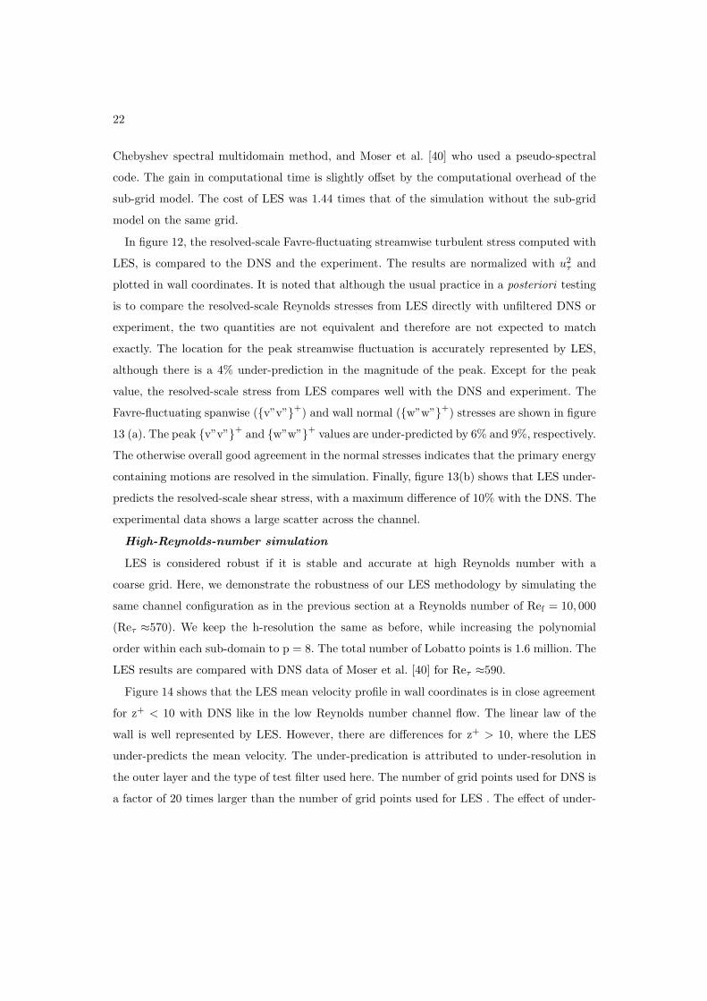
Figure 14 shows that the LES mean velocity profile in wall coordinates is in close agreement

for z+ < 10 with DNS like in the low Reynolds number channel flow. The linear law of the

wall is well represented by LES. However, there are differences for z+ > 10, where the LES

under-predicts the mean velocity. The under-predication is attributed to under-resolution in

the outer layer and the type of test filter used here. The number of grid points used for DNS is

a factor of 20 times larger than the number of grid points used for LES . The effect of under-

23

resolution was investigated in several studies. In Bagget et al. [43] the resolution requirement

for LES of shear flows using the dynamic Smagronsky model was studied through a series of

channel flow simulations at high Reynolds number (Reτ ≈ 1000). They varied the resolution

in the outer-layer while keeping the near wall mesh the same, which essentially resolved the

near wall structures. It was shown that the sub-grid shear stress predicted by the dynamic

model in posteriori simulation, was less than the shear stress obtained using filtered DNS data.

Such under-prediction in shear stress directly affects the averaged velocity profile. Using the

data from [43], Jimenez and Moser [44] showed that the fractional error in prediction of mean

velocity is roughly proportional to and is of the same order as the fraction of shear stress

carried by the sub-grid model. Therefore, they concluded that the prediction in mean velocity

can be improved by adjusting the resolution so that the amount of shear stress carried by

the sub-grid model is small. Under-prediction in the averaged velocity was also observed by

Blackburn and Schmidt [11], for their spectral element LES using interpolant-projection type

filtering.

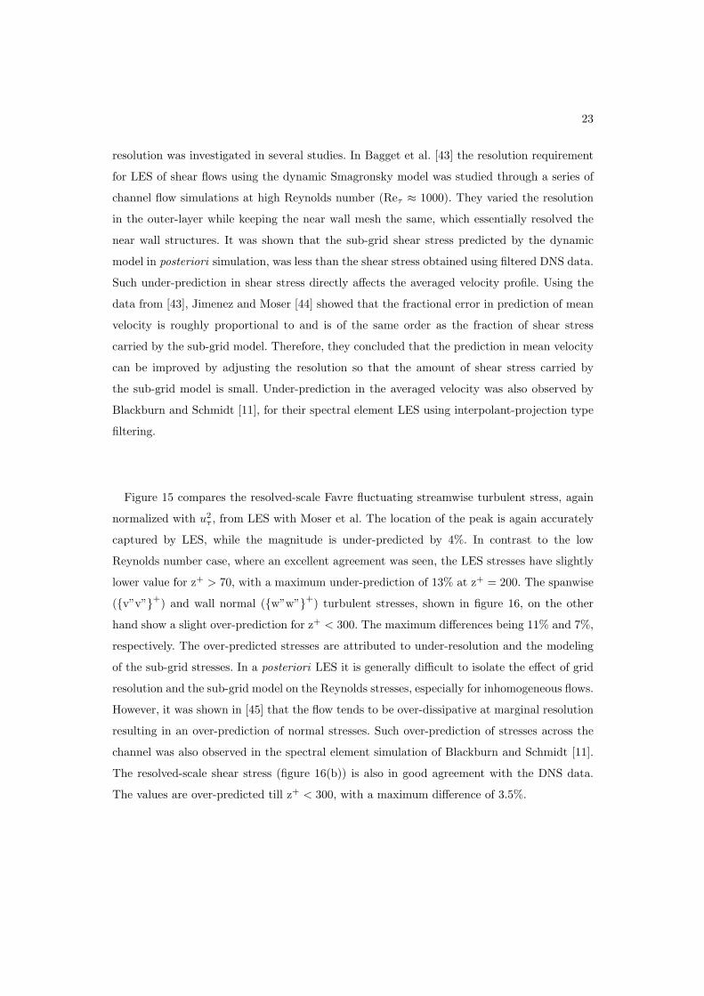
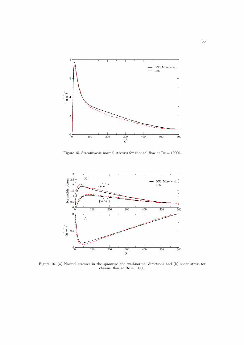
Figure 15 compares the resolved-scale Favre fluctuating streamwise turbulent stress, again

normalized with u2τ , from LES with Moser et al. The location of the peak is again accurately

captured by LES, while the magnitude is under-predicted by 4%. In contrast to the low

Reynolds number case, where an excellent agreement was seen, the LES stresses have slightly

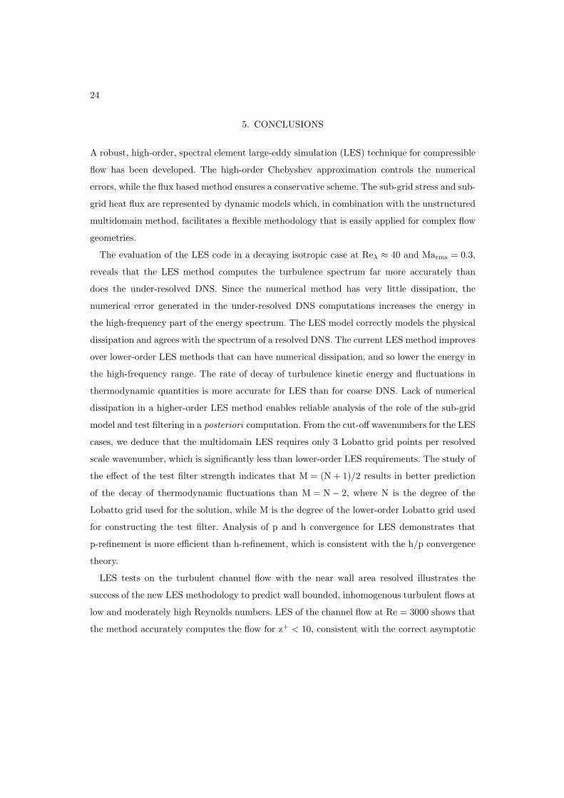
lower value for z+ > 70, with a maximum under-prediction of 13% at z+ = 200. The spanwise

(v”v”+) and wall normal (w”w”+) turbulent stresses, shown in figure 16, on the other

hand show a slight over-prediction for z+ < 300. The maximum differences being 11% and 7%,

respectively. The over-predicted stresses are attributed to under-resolution and the modeling

of the sub-grid stresses. In a posteriori LES it is generally difficult to isolate the effect of grid

resolution and the sub-grid model on the Reynolds stresses, especially for inhomogeneous flows.

However, it was shown in [45] that the flow tends to be over-dissipative at marginal resolution

resulting in an over-prediction of normal stresses. Such over-prediction of stresses across the

channel was also observed in the spectral element simulation of Blackburn and Schmidt [11].

The resolved-scale shear stress (figure 16(b)) is also in good agreement with the DNS data.

The values are over-predicted till z+ < 300, with a maximum difference of 3.5%.

24

5. CONCLUSIONS

A robust, high-order, spectral element large-eddy simulation (LES) technique for compressible

flow has been developed. The high-order Chebyshev approximation controls the numerical

errors, while the flux based method ensures a conservative scheme. The sub-grid stress and sub-

grid heat flux are represented by dynamic models which, in combination with the unstructured

multidomain method, facilitates a flexible methodology that is easily applied for complex flow

geometries.

The evaluation of the LES code in a decaying isotropic case at Reλ ≈ 40 and Marms = 0.3,

reveals that the LES method computes the turbulence spectrum far more accurately than

does the under-resolved DNS. Since the numerical method has very little dissipation, the

numerical error generated in the under-resolved DNS computations increases the energy in

the high-frequency part of the energy spectrum. The LES model correctly models the physical

dissipation and agrees with the spectrum of a resolved DNS. The current LES method improves

over lower-order LES methods that can have numerical dissipation, and so lower the energy in

the high-frequency range. The rate of decay of turbulence kinetic energy and fluctuations in

thermodynamic quantities is more accurate for LES than for coarse DNS. Lack of numerical

dissipation in a higher-order LES method enables reliable analysis of the role of the sub-grid

model and test filtering in a posteriori computation. From the cut-off wavenumbers for the LES

cases, we deduce that the multidomain LES requires only 3 Lobatto grid points per resolved

scale wavenumber, which is significantly less than lower-order LES requirements. The study of

the effect of the test filter strength indicates that M = (N + 1)/2 results in better prediction

of the decay of thermodynamic fluctuations than M = N− 2, where N is the degree of the

Lobatto grid used for the solution, while M is the degree of the lower-order Lobatto grid used

for constructing the test filter. Analysis of p and h convergence for LES demonstrates that

p-refinement is more efficient than h-refinement, which is consistent with the h/p convergence

theory.

LES tests on the turbulent channel flow with the near wall area resolved illustrates the

success of the new LES methodology to predict wall bounded, inhomogenous turbulent flows at

low and moderately high Reynolds numbers. LES of the channel flow at Re = 3000 shows that

the method accurately computes the flow for z+ < 10, consistent with the correct asymptotic

25

variation of the sub-grid length scale with the distance from the wall as enforced by the dynamic

Smagorinsky model. LES under-predicts peak value of normal stresses, also consistent with the

predictions of LES based on finite difference methods. Since the multidomain method is not

dissipative, the under-prediction is attributed to the under-dissipative nature of the dynamic

model.

The LES methodology was shown to be robust, i.e. it is able to predict high-Reynolds

number flows with fair accuracy on a relatively coarse grid. Robustness was demonstrated by

a simulation of the channel flow at Re = 10, 000. The mean flow and the Reynolds stress are in

fair agreement with the published DNS result. The dynamic model is known to under-predict

the sub-grid shear stresses in turbulent channel flows, especially at high Reynolds numbers.

This leads to error in the prediction of averaged velocity unless the resolution is increased

sufficiently to reduce the proportion of the shear stress carried by the model. The marginal

resolution in our simulation, results in under-prediction of the average velocity in the outer

layer at z+ > 10 and larger deviation of the Reynolds stresses compared to the low Reynolds

number case.

With tests on the isotropic turbulence and the turbulent channel flow, the characteristics

of the LES methodology have been exposed. Further research is currently underway to apply

the methodologies presented here, for simulation of more complex flows like the flow over a

backward-facing step, where the method is expected to improve over most other LES numerical

schemes.

The multidomain spectral method is of the same type as the discontinuous Galerkin method

and discontinuous finite element method. The conclusion and observations from this paper

thus extend to this broader class of numerical methods.

ACKNOWLEDGEMENTS

The support for this work was provided by the U.S. Office of Naval Research with Dr. G.D. Roy asthe Program Officer. Computational time was provided in part by National Center for SupercomputingApplications (NCSA).

REFERENCES

1. Ghosal S. An analysis of numerical errors in large-eddy simulations of turbulence. Journal of Comput.Physics 1996; 125:187–206.

26

2. Kravchenko AG, Moin P. On the effect of numerical errors in large eddy simulation of turbulent flows.Journal of Comput. Physics 1997; 131:310–322.

3. Bui TT. A parallel, finite volume algorithm for large-eddy simulation of turbulent flows. Computer andFluids 2000; 29:877–915.

4. Mahesh K, Constantinescu G, Moin P. A numerical method for large-eddy simulation in complexgeometries. Journal of Comput. Physics 2004; 197:215–240.

5. Jansen K. A stabilized finite element method for computing turbulence. Comput. Methods. Appl. Mech.Engrg 1999; 174:299–317.

6. Santhanam S, Lele SK, Ferziger JH. A robust high-order compact method for large-eddy simulation.Journal of Computational Physics 2003; 191:392–419.

7. Blaisdell GA, Spyropoulos ET, Qin JH. The effect of the formulation of nonlinear terms on aliasing errorsin spectral methods. Appl. Numer. Math. 1996; 21:207.

8. Moin P, Squires K, Cabot W, Lee S. A dynamic subgrid model for compressible turbulence and scalartransport. Phys. Fluids A 3 1991; 11:2746–2757.

9. Karniadakis GEM, Sherwin S. Spectral/hp Element Methods for Computational Fluid Dynamics. OxfordUniversity Press: New York, USA, 2005.

10. Deville MO, Fischer PF, Mund EH. High-Order Methods for Incompressible Fluid Flow. CambridgeUniversity Press: Cambridge, UK, 2002.

11. Blackburn HM, Schmidt S. Spectral element filtering techniques for large eddy simulation with dynamicestimation. Journal of Computational Physics 2003; 186:610–629.

12. Fischer PF, Mullen JS. Filter based stabilization of spectral element methods. Comptes Rendus al’Academie des Sciences Paris, Ser. 1, Anal. Numer 2001; 332:265–270.

13. Levin JG, Iskandarani M, Haidvogel DB. A spectral filtering procedure for eddy-resolving simulations witha spectral element ocean model. Journal of Computational Physics 1997; 137:130–154.

14. Karamanos GS. Large eddy simulation using unstructured spectral/hp finite elements. PhD Thesis,Imperial College, London 1999.

15. Karamanos GS, Karniadakis GE. A spectral vanishing viscosity method for large-eddy simulations. Journalof Comput. Physics 2000; 163:22–50.

16. Jacobs GB, Kopriva DA, Mashayek F. Validation study of a multidomain spectral code for simulation ofturbulent flows. AIAA Journal 2005; 43(6):1256–1264.

17. Kopriva DA, Kolias JH. A conservative staggared-grid Chebyshev multidomain method for compressibleflows. Journal of Comput. Physics 1996; 125:244–261.

18. Kopriva DA. A staggared-grid multidomain spectral method for compressible Navier-Stokes equations.Journal of Comput. Physics 1998; 143:125–158.

19. Jacobs GB. Numerical simulation of two-phase turbulent compressible flows with a multidomain spectralmethod. PhD Thesis, University of Illinois at Chicago, Chicago 2003.

20. Vreman B, Guerts B, Kuerten H. Subgrid-modeling in LES of compressible flow. Appl. Sci. Res. 1995;54:191–203.

21. Vreman B, Guerts B, Kuerten H. Large-eddy simulation of turbulent mixing layers. Journal of FluidMechanics 1997; 339:357–390.

22. Germano M, Piomelli U, Moin P, Cabot WH. A dynamic subgrid scale eddy viscosity model. Phys. FluidsA 3 1991; 7:1760–1765.

23. Yoshizawa A. Statistical theory for compressible turbulent shear flows, with the application to subgridmodeling. Physics of Fluids A 1986; 29(7):2152–2164.

24. Erlebacher G, Hussaini MY, Speziale CG, Zang TA. Toward the large-eddy simulation of compressibleturbulent flows. Journal of Fluid Mechanics 1992; 238:155–185.

25. Squires KD. Dynamic subgrid scale modeling of compressible turbulence. Annual Research Brief, StanfordUniversity 1991.

26. Vreman AW, Guerts BJ, Kuerten J. Direct and large-eddy simulation I. Kluwer academic publisher:Netherlands, 1994.

27. Okong’o N, Knight DD, Zhou G. Large-eddy simulations using an unstructured grid compressible Navier-Stokes algorithm. International Journal of Computational Fluid Dynamics 2000; 13(4):303–326.

28. Lily DK. A proposed modification of the Germano subgrid-scale closure method. Phys. Fluids A 4 1992;3:633–635.

29. Bardina J, Ferziger JH, Reynolds WC. Improved turbulence models based on large eddy simulationof homogeneous, incompressible, turbulent flows. Report, Thermosciences Division, Dept. MechanicalEngineering TF-19, Stanford University 1983.

30. Rogallo RS. Numerical experiments in homogeneous turbulence. NASA Report TM 81315, NASA 1981.31. Blaisdell GA, Mansour NN, Reynolds WC. Compressibility effects on the growth and structure of

homogeneous turbulent shear flow. Journal of Fluid Mechanics 1993; 256:443–485.32. Smits AJ, Dussage JP. Turbulent Shear Layers in Supersonic Flow. Springer: Springer, 2006.

27

33. Piomelli U. Large-eddy simulation: achievements and challenges. Progress in Aerospace Sciences 1999;35:335–362.

34. Moin P, Kim J. Numerical investigation of turbulent channel flow. Journal of Fluid Mechanics 1982;118:341–377.

35. Piomelli U. High Reynolds number calculations using the dynamic subgrid-scale stress model. Phys. FluidsA 1993; 5(6):1484–1490.

36. Wang WP, Pletcher RH. On the large eddy simulation of a turbulent channel flow with significant heattransfer. Physics of Fluids 1996; 8(12):3354–3366.

37. Lenormand E, Sagaut P, Ta Phuoc T. Large eddy simulation of subsonic and supersonic channel flow atmoderate Reynolds number. Int. J. Numer. Meth. Fluids 2000; 32:369–406.

38. Jacobs GB, Kopriva DA, Mashayek F. A conservative isothermal wall boundary condition for thecompressible Navier-Stokes equation. Journal of Scientific Computing 2007; 30(2):177–192.

39. Ridder JP, Beddini R. Large eddy simulation of compressible channel flow. NASA Tech. Report NGT-50363, NASA 1993.

40. Moser R, Kim J, Mansour NN. Direct numerical simulation of turbulent channel flow up to Reτ = 590.Physics of Fluids 1999; 11(4):943–945.

41. Niederschulte MA, Adrian RJ, Hanratty TJ. Measurements of turbulent flow in a channel at low Reynoldsnumbers. Exp. Fluids 1990; 9:222–230.

42. Zhao H, Voke PR. A dynamic subgrid-scale model for low-Reynolds number channel flow. InternationalJournal for Numerical Methods in Fluids 1996; 23:19–27.

43. Bagget JS, Jimenez J, Kravchenko AG. Resolution requirements in large-eddy simulation of shear flows.Annual Research Briefs, Center for Turbulence Research, Stanford University, Stanford, CA 1997.

44. Jimenez J, Moser RD. Large-eddy simulations: where are we and what can we expect? AIAA Journal2000; 38(4):605–612.

45. Najjar FM, Tafti DK. Study of discrete test filter and finite difference approximations for the dynamicsubgrid-scale stress model. Physics of Fluids 1996; 8(4):1076–1088.

Table I. Cases for decaying isotropic turbulence simulation.

Case hx × hy × hz p M

DNS-RES 6× 6× 6 15 NA

DNS-URES 6× 6× 6 8 NA

LES-BASE 6× 6× 6 8 (N+1)/2

LES-RFNDp 6× 6× 6 10 (N+1)/2

LES-FILT 6× 6× 6 8 N-2

LES-RFNDh 7× 7× 7 8 (N+1)/2

28

X

Z

Y

Figure 1. Staggared arrangement of solution variable and fluxes, closed circles: ggg points, opensquares: lgg points, open circles: glg points, closed squares: ggl points.

1 10k

1e-06

0.0001

E(k

)

DNS, Blaisdel et al.DNS-RESDNS-URESLES-BASELES-RFNDp

1 10k

1e-08

1e-07

1e-06

1e-05

0.0001

0.001

D(k

)

(b)(a)

Figure 2. Comparison of (a) energy spectra and (b) dissipation spectra at t=3.2 for isotropicturbulence.

29

10k

1e-05

0.0001

0.001

E(k

)DNS, Blaisdel et al.DNS-RESDNS-URESLES-BASELES-RFNDp

10k

1e-05

0.0001

0.001

D(k

)

(a) (b)

Figure 3. Same as figure 2, zoomed in on high wave-numbers.

0 2 4 6 8t

0

0.01

0.02

0.03

0.04

0.05

TK

E

DNS-RESDNS-URESLES-BASE

0 0.5 1 1.5 2t

-20

-10

0

10

20

% R

elat

ive

Err

or

Figure 4. Decay of turbulent kinetic energy for isotropic turbulence. Inset: relative error for casesLES-BASE and DNS-URES.

30

1 10k

1e-08

1e-06

0.0001

0.01E

s(k)

1 10k

1e-08

1e-07

1e-06

1e-05

0.0001

Ed(k

)

DNS, Blaisdel et al.DNS-RESDNS-URESLES-BASEDNS, p=20

(a) (b)

Figure 5. Comparison of decomposed energy spectra at t=3.2 for isotropic turbulence: (a) solenoidalspectrum (b) dilatational spectrum.

0 1 2 3 4 50

0.001

0.002

0.003

<p’ p’ >

/(γ2 <

p>2 ) DNS-RES

LES-BASEDNS-URES

0 1 2 3 4 5tε0/k0

0

0.001

0.002

0.003

<ρ’ ρ’ >

/(γ2 <

ρ>2 )

(a)

(b)

Figure 6. Decay of (a) pressure and (b) density fluctuations.

31

0 2 4 6 8t

0

0.01

0.02

0.03

0.04

0.05

TK

EDNS-RESLES-BASELES-FILT

0 0.5 1 1.5 2t

-4

-2

0

2

4

% R

elat

ive

Err

or

Figure 7. Decay of turbulent kinetic energy, for DNS and LES with different test filter strengths. Inset:relative error for cases LES-BASE and LES-FILT.

0 1 2 3 4 50

0.001

0.002

0.003

<p’ p’ >

/(γ2 <

p>2 ) DNS-RES

LES-BASELES-FILT

0 1 2 3 4 5tε0/k0

0

0.001

0.002

0.003

<ρ’ ρ’ >

/(γ2 <

ρ>2 )

(a)

(b)

Figure 8. Decay of (a) pressure and (b) density fluctuations, for DNS and LES with different test filterstrengths.

32

10k

1e-05

0.0001

0.001

E(k

)DNS, Blaisdel et al.DNS-RESLES-BASELES-RFNDpLES-RFNDh

10k

1e-05

0.0001

0.001

D(k

)

(a) (b)

Figure 9. h/p resolution study: (a) energy spectra and (b) dissipation spectra.

2

2 6

x

z

y

Figure 10. Schematic of channel flow geometry (not to scale).

33

1 10 100

Z+

0

5

10

15

20

U+

DNS, Moser et al.LES, p=6Law of the wall

Figure 11. Mean normalized streamwise velocity plotted in wall coordinates for channel flow atRe = 3000.

0 50 100 150

z+

0

2

4

6

8

u" u" +

Exp., Nierdershulte et al.DNS, Moser et al.LES, p=6

Figure 12. Streamswise normal stresses for channel flow at Re = 3000.

34

0 50 100 1500

0.5

1

1.5

Rey

nold

s St

ress

Exp., Nierdershulte et al.DNS, Moser et al.LES, p=6

0 50 100 150

z+

-0.8

-0.6

-0.4

-0.2

0

u" w

" +v

"v

"

w"w

"

(a)

(b)

Figure 13. (a) Normal stresses in the spanwise and wall-normal directions and (b) shear stress forchannel flow at Re = 3000.

1 10 100

Z+

0

5

10

15

20

25

30

U+

DNS, Moser et al.LESLaw of the wall

Figure 14. Mean normalized streamwise velocity plotted in wall coordinates for channel flow atRe = 10000.

35

0 100 200 300 400 500 600

Z+

0

2

4

6

8

u" u" +

DNS, Moser et al.LES

Figure 15. Streamswise normal stresses for channel flow at Re = 10000.

0 100 200 300 400 500 6000

0.5

1

1.5

2

2.5

3

Rey

nold

s St

ress DNS, Moser et al.

LES

0 100 200 300 400 500 600

Z+

-1

-0.5

0

u" w

" +

(a)

(b)

v"v

"

+

w"w

"

+

Figure 16. (a) Normal stresses in the spanwise and wall-normal directions and (b) shear stress forchannel flow at Re = 10000.