Embed Size (px)
Citation preview
Large-Scale Evaluations of Curricular Effectiveness:
The Case of Elementary Mathematics in Indiana
Rachana Bhatt
Georgia State University
Cory Koedel*
University of Missouri
January 2012
We use data from one of the few states where information on curriculum
adoptions is available – Indiana – to empirically evaluate differences in
performance across three elementary-mathematics curricula. The three
curricula that we evaluate were popular nationally during the time of our study,
and two of the three remain popular today. We find large differences in
effectiveness between the curricula, most notably between the two that held the
largest market shares in Indiana. Both are best-characterized as traditional in
pedagogy. We also show that the publisher of the least-effective curriculum
did not lose market share in Indiana in the following adoption cycle; one
explanation is that educational decision makers lack information about
differences in curricular effectiveness.
* We thank Emek Basker, Julie Cullen, Gordon Dahl, Barry Hirsch, Josh Kinsler, David Mandy,
Peter Mueser, Rusty Tchernis and many seminar and conference participants for useful
comments and suggestions. We also thank Karen Lane and Molly Chamberlin at the Indiana
Department of Education for help with data. This work was not funded or influenced by any
outside entity.
1
I. Introduction
According to a 2002 survey sponsored by the National Education Association and the
American Association of Publishers, 80 percent of teachers use textbooks in the classroom and
over half of students’ in-class instructional time involves textbook use (Finn, 2004).1 Braswell et
al. (2001) report that 56 percent of fourth graders do math problems from their textbooks every
day. Given the central role that curriculum materials play in the education production process, it
stands to reason that differences across curricula in terms of content, organization, and pedagogy
can lead to differences in student achievement. This sentiment is echoed in a recent research
brief from the National Council of Teachers of Mathematics, which notes that selecting a math
curriculum is “one of the most critical decisions educational leaders make.” (NCTM, 2009)
The curriculum market is diverse – in the case of elementary mathematics, for example,
the What Works Clearinghouse (WWC) has identified over 70 different curriculum options.2 But
there are few rigorous, empirical evaluations of curricular effectiveness; the research literature is
surprisingly thin. One reason is that most state education agencies do not provide information
about which curricula are used in which schools and districts. In fact, many states do not collect
centralized data at all. The lack of data prevents empirical analyses, and as a result there is little
in the way of reliable evidence on curricular effectiveness (Slavin and Lake, 2008; WWC, 2007).
This limits the ability of educational administrators to make informed curriculum-adoption
decisions.
This study makes two contributions to the research literature on curricular effectiveness.
First, we use data from one of two states that track curriculum adoptions over time (Indiana) to
estimate differences in effectiveness between three elementary-mathematics curricula. Each of
1 Textbooks are just one component of the curricula purchased by schools from publishers. Other materials include
teacher instructional support services and supplementary materials such as student workbooks and solution manuals. 2 Note that some of these are inactive or discontinued, but nonetheless, many active options are available.
2
the curricula had large, national market shares during the time of our study (1998-2004), and two
of the three have large market shares today. The three curricula differ in organization and
pedagogy, and share similarities with other curricula that we do not evaluate directly. A notable
and ongoing disagreement in the literature is between advocates of “traditional” and “reform”
approaches to mathematics instruction. A key insight from our analysis is that there can be large
differences in effectiveness between curricula that share the same pedagogical approach.
A second contribution of our study relates to the larger issue that the research literature in
this area is so thin. There are too many curriculum options within any given subject-grade group,
including elementary mathematics, for a single study to cover them all. Moreover, a single study
cannot replicate the variety of educational environments in which curricula are used, which is
important given that curricula may perform differently in different contexts. But a series of
independent evaluations from multiple contexts, taken together, could provide valuable
information about the effectiveness of the various curricular alternatives. With this in mind, we
provide extensive technical details regarding our evaluation so that it can be used as a resource
for future, similar studies (some of these details are provided in the online appendix: [EEPA link
here]). Every evaluation environment will be different, but empirical studies along the lines of
what we present here are likely to be feasible in many states. Furthermore, they would be
relatively inexpensive to perform. If state education agencies would simply begin collecting data
on curriculum adoptions, and make these data available, studies could be produced that would
arm decision makers with valuable information on this important topic.
We highlight two key findings from this particular evaluation. First, we identify
statistically significant and meaningful differences in curriculum performance as measured by
school-level test scores on the Indiana state test (ISTEP). We find the most substantial
3
differences between two curricula that use the same pedagogical approach (traditional) but differ
in other respects. Although much attention is devoted to the debate over traditional- versus
reform-based mathematics instruction, our findings suggest that other differences in curriculum
design are substantively important. A second key result is that the publisher of the curriculum we
found to be least-effective did not lose market share in the following adoption cycle in Indiana.
There are several potential explanations for this result. Perhaps the most compelling is that
decision makers have virtually no information about which curricula are most effective.3
II. Background
To the best of our knowledge only two states – Indiana and Florida – make current and
historical information on curriculum adoptions publicly available. Many states do not track
curriculum adoptions at all, making it impossible to perform empirical analyses that can inform
decision makers. This is an issue that can be easily remedied moving forward, and we argue that
it should be remedied; but the current data infrastructure in most states makes large-scale
empirical investigations of curricular effectiveness infeasible.
In the present study we use the Indiana data to estimate relative curriculum effects for the
three most commonly adopted elementary-mathematics curricula in the state during the 1998-
2004 curriculum-adoption cycle.4 These three curricula – Saxon Math (Saxon), Silver-Burdett
Ginn Mathematics (SBG), and Scott Foresman-Addison Wesley (SFAW) – accounted for 86
percent of all curriculum adoptions in Indiana during our study. All three were popular outside of
Indiana as well, and used in other states including California, Florida, Louisiana, Tennessee and
Texas (Educational Marketer; 1998a,b; 1999a,b). And two of the three remain popular today.
The exception is SBG, which was bought by the publisher of SFAW and ultimately discontinued.
3 An alternative explanation is that educational administrators do not consistently make optimal decisions in general.
For example, see Ballou’s (1996) study on teacher hiring. 4 We focus on this adoption cycle to maximize the number of cohorts whose achievement data we observe.
4
Curriculum Descriptions
The three curricula share similarities with other curricula that are widely circulated. For
instance, Saxon and SBG both are best described as “traditional” in pedagogy. Both emphasize
teacher-led instruction where students receive step-by-step guidance for problem solving and are
drilled in implementation. Singapore Math, a curriculum that is gaining popularity in schools
across the United States, takes a similar pedagogical approach (WWC, 2007). Alternatively,
SFAW is best characterized as a blend of “traditional” and “reform” instruction. Reform-based
curricula emphasize student inquiry, real-world applications of problems, and the use of visual
aids for understanding.5 Recent research suggests that reform-based instruction can be highly
effective (e.g., Riordan and Noyce, 2001; WWC, 2007), and SFAW shares similarities with
popular reform-based curricula including Everyday Mathematics (WWC, 2007).
There are many other differences between the curricula beyond the dimension of
pedagogy, which we highlight in comparative reviews below. Our reviews draw on information
from the WWC, the publishers themselves, several research studies, and a curriculum advocacy
group (Mathematically Correct).6 They reveal four main differences between the curricula: (1)
Saxon presents related material in incremental units (distributive approach), whereas SBG and
SFAW present related material in self-contained units (massed approach), (2) SBG structures
lessons by interweaving examples and student practice, (3) the “reform” elements of SFAW
include an emphasis on real-world examples and conceptual understanding before technical
details, and (4) Saxon does not cover some higher-order topics covered by the other curricula.
5 Further discussion can be found in Agodini et al. (2010), National Mathematics Advisory Panel (2007, 2008) and
An (2004). These sources describe what is perhaps best viewed as a continuum of curriculum options with endpoints
at “purely traditional” and “purely reform.” Most curricula fall somewhere in-between. 6 The information that we obtained from the WWC and the research literature is likely the most objective. The
information from the publishers and Mathematically Correct is likely the least objective. We try to avoid carrying
over subjective curriculum descriptions when we can. Note that in some cases the reviews are for different editions
of the curricula; however, we expect within-curriculum, across-edition differences to be small.
5
Saxon Math
The WWC (2007) describes instruction to students in Saxon Math as “incremental and
explicit,” and based on “teacher-directed conversations.” Slavin and Lake (2008) similarly
describe Saxon Math as “traditional” and “algorithmically focused.” Saxon provides teachers
with scripts for each lesson, and teachers are directed to structure daily lessons in three parts.
First, teachers review prior concepts with students, usually through an interactive activity. Next
they introduce new concepts, and teach students exact methods for solving problems. Finally,
students practice solving problems in class. Students are assigned homework to be completed
individually and assessments are given every five lessons (Agodini et al., 2010; Slavin and Lake,
2008). Continued practice and review is a key aspect of Saxon (Bolser and Gilman, 2003).
A feature of the Saxon curriculum that differentiates it from the other two curricula is its
use of the distributed approach to presenting related material (WWC, 2007; HMHP, 2008). That
is, for a given topic, instruction and assessment on the topic is distributed throughout the
academic year in incremental phases, rather than in a single setting. For instance, when students
are taught how to tell time in grade-2, they are first taught how to tell time to the hour, then move
on to another subject, return back to time and learn half hour increments, move on, learn five
minute increments, move on again, and finally learn how to tell time to the minute level.7 This is
in stark contrast to how SBG and SFAW teach time – both use a massed approach where all
concepts related to time are taught without interruption in a self-contained unit (Ellis, 2006).
Silver-Burdett Ginn Mathematics
SBG is also best classified as a traditional mathematics curriculum. A 1999 review from
Mathematically Correct describes SBG as providing material to students in a structured way,
7 Prior research suggests that the distributed approach increases the amount of information that students retain and
understand (Bloom and Shuell, 1981; Rea and Modigliani, 1985).
6
similarly to Saxon.8 Teachers first introduce a topic to the class and students participate in small-
group or whole-class activities on the topic. Students are then tested using book problems.
Teachers re-assess student understanding with another activity, followed by student practice.
While Saxon and SBG fall on the same end of the traditional/reform spectrum, three
notable differences became apparent during our review. First, as noted above, SBG uses a
massed approach to instruction whereas Saxon uses a distributive approach. Second, SBG
focuses more on group work, and interweaves class or small group activities with individual
practice. This is in contrast to presenting all examples upfront and then having students practice
afterward.9 Finally, SBG presents higher-order material for some topics that is not presented in
Saxon. As an example, the grade-2 SBG curriculum covers addition and subtraction for three-
digit numbers, whereas Saxon only covers addition and subtraction up to two-digit numbers.10
Scott-Foresman Addison Wesley Math
SFAW offers a blend between the traditional and reform approaches to mathematics
instruction. A traditional feature of the curriculum is that it encourages students to practice,
although there are no “drills” per se. Instead, teachers are directed to structure lessons in a check-
learn-check-practice format. First, teachers check student knowledge about a particular concept,
then introduce new concepts, then check their understanding, and then students practice
problems from the text. The problems are designed to be real-world oriented in the reform-based
mold. The organization of SFAW also highlights the “reform” aspect of the curriculum. For
8 We had difficulty obtaining information about the SBG curriculum because it has been discontinued. We primarily
draw on Mathematically Correct (MC), an advocacy group in favor of traditional-based mathematics instruction, for
our review here. MC is not an objective source, but we do our best to pull only objective information. We also note
that any bias from MC’s pedagogical preference is less likely to be an issue when comparing Saxon and SBG since
both are traditional-based. More information is available at: http://www.mathematicallycorrect.com. 9 Previous research shows that interspersing examples with practice is an effective organizational tool for student
learning (Sweller and Cooper, 1985; Trafton and Reiser, 1993). 10
The current edition of Saxon Math covers three-digit addition and subtraction, however the edition studied here
did not. For more information: http://saxonpublishers.hmhco.com/HA/correlations/pdf/s/SM_2_NA_TOC.pdf).
7
example, when covering one-digit addition and subtraction, SFAW first devotes an entire unit to
conceptual understanding and recognizing patterns, and then lays out strategies for problem
solving, whereas SBG and Saxon teach problem-solving strategies upfront.
The WWC report also indicates that the SFAW curriculum is well-designed for use by
students of differing ability levels. Correspondingly, it covers higher-order topics not covered by
Saxon, similarly to SBG. A final notable feature of SFAW is that it uses of a variety of different
instructional materials including transparencies, workbooks and technology (Agodini et al.,
2010; Resendez and Manley, 2005; WWC, 2007).11
Curriculum Selection Process in Indiana
Curriculum adoptions occur annually in Indiana and rotate in six-year cycles by subject.
For example, Indiana’s districts adopted new math curricula in 1998, 2004, and 2010. Similarly,
recent reading adoptions occurred in 1994, 2000 and 2006. We focus our evaluation on the math-
curriculum adoption that occurred in 1998, and on adoptions in grades 1, 2 and 3.
The adoption process has centralized and decentralized components. It begins in July of
the year prior to the new adoption (for the cycle where the new curricula were first used in the
fall of 1998, this was July 1997). First, there is a four month review of the curriculum options by
an official Textbook Advisory Committee (TAC) at the Indiana DOE (state level). By October,
the TAC compiles a list of approved curricula and distributes this list to school districts. At this
point the review process becomes decentralized and varies from district to district, but a common
approach is for a district to form a committee of administrators, parents, and teachers to review
the material and recommend a curriculum. The general public is also typically given an
opportunity to comment. Overall, the district portion of the review process lasts for roughly 9
11
Several studies suggest that combining verbal descriptions with visual aids is an effective instructional practice
(Mayer and Anderson, 1992; Mayer, 2001).
8
months and involves many individuals in different capacities. Each district makes a final
decision in the summer before the new curricula are used in classrooms.12
At the conclusion of the process districts make one of three decisions. First, and most
commonly, they choose to adopt one or more of the state-approved curricula. Second, they may
apply to use alternative curricula that are not on the list, but this rarely happens in practice (e.g.,
no more than one out of the roughly 300 districts chooses this option in any grade in our data).
Third, districts can apply for “continued use” where they quite literally continue to use the old
textbooks from the prior adoption cycle. Over 98 percent of the districts in Indiana adopted new
math curricula from the approved list during the 1998 adoption cycle.
III. Data
We construct a 17-year data panel of schools and districts for our analysis. The data
include information about curriculum adoptions along with detailed school- and district-level
information on student achievement, attendance, enrollment, demographics, and financing. We
perform our primary analysis at the school level.
Our data panel starts with the 1991-1992 school year and ends in 2007-2008. The
curricula of interest were first used in schools in the fall of 1998, and replaced in the fall of 2004.
We observe seven cohorts of grade-3 students who were never exposed to the curricula during
the pre-period (1991-1992 through 1997-1998), one cohort that was exposed in grade three only
(1998-1999), one cohort that was exposed in grades two and three only (1999-2000), four
cohorts that used the curricula in all three grades and were thus “fully exposed” (2000-2001
through 2003-2004), one cohort that was exposed in grades one and two only (2004-2005), one
cohort that was exposed in grade one only (2005-2006), and two cohorts in the post period
(2006-2007 and 2007-2008) that were never exposed. They key cohorts of interest are the
12
For an example of a district review process, see http://www.munster.k12.in.us/ParentHandout.pdf.
9
cohorts that were directly exposed to the curricula that we evaluate. We use the unexposed
cohorts to perform falsification tests, which allow us to investigate the extent to which our
primary findings are likely to be biased (see Section VII).
Our measure of achievement is the Indiana Statewide Testing for Educational Progress
(ISTEP) exam. The ISTEP is a standards-based, criterion-referenced test administered in math
and language arts. During most of our data panel it was administered in grades 3, 6, 8, and 10
(more recently it has been given annually in grades 3-8). The math ISTEP assesses student skills
in the following areas: number sense, computation, algebra, geometry, measurement, and
problem solving. Student scores on the ISTEP are reported in scale scores, and the tests are
constructed to measure student knowledge of the core concepts and practices outlined in the
Indiana DOE standards. Given that the DOE standards for mathematics are a major factor in the
curriculum selection process, and that the ISTEP is designed to test mastery of these standards,
the test should be well-suited to evaluate the relative effectiveness of the three curricula.13
ISTEP scores are first available for analysis in grade-3, and grade-3 scores are a function
of the curricula to which students are exposed in earlier grades as well. Therefore, our estimates
are best viewed as characterizing the impacts of sequences of curriculum treatments. To allow
for cleanly identified effects we exclude districts that adopted more than one curriculum across
grades 1-3. To illustrate the assignment problem in such circumstances, consider a district that
adopted Saxon in grade one and SBG in grades two and three. In identifying the effect of Saxon
relative to SBG, schools in this district are not well-defined as either treatments or controls. We
refer to districts that used the same curriculum in all three grades as “uniform curriculum
adopters.” Restricting our analysis to these districts reduces our district sample size by eight
percent and our school sample size by seven percent (see Appendix Table C.1). After restricting
13
Perhaps the most Indiana-specific feature of our study is that we measure outcomes using the ISTEP. Our results
may not extend to settings where the testing instrument differs a great deal from the ISTEP, although we note that
the core concepts that are tested on the ISTEP are common math concepts nationally.
10
our sample we are left with data from 213 districts and 716 schools. By a large margin, this
makes our study the largest curriculum evaluation of which we are aware.14
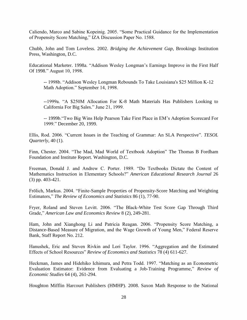
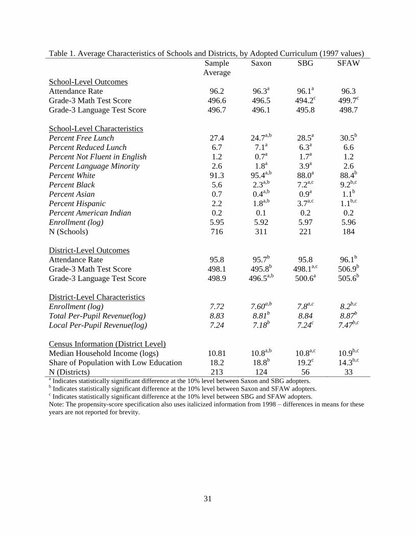
In Table 1 we report differences in means across the schools and districts that adopted
different curricula prior to adoption (1997). There are only small differences in test scores and
attendance across curriculum adopters. There are larger differences in school demographics,
district size, and to some extent, median household income. But even in some cases where the
differences are statistically significant they are substantively small. Overall, the descriptive
statistics in Table 1 are encouraging because the differences across curriculum adopters imply
considerable overlap in the distributions of characteristics across treatment groups. This is a key
condition for the successful implementation of our empirical strategy, which we discuss further
in Section IV.
A final data issue relates to the long duration of our study. Specifically, over the 17 years
of our data panel the composition of schools in Indiana changed to some degree (due to school
closings). This issue will almost surely come up in other large-scale curriculum evaluations
given the typically long duration of implementation.15
The key issue is whether changes in the
composition of schools are correlated with curriculum adoptions – if they are, they can introduce
bias into the evaluation. We discuss this issue in detail in the appendix– we find no evidence to
suggest that compositional changes in our sample over time bias our findings.
IV. Empirical Strategy
School-level Matching Estimators
We use school-level matching estimators to estimate the curriculum effects. Matching is
an increasingly common empirical technique, and the conditions under which matching will
14
The largest experimental study of which we are aware is by Agodini et al. (2010), which examines four curricula
in over 100 schools. More typically, experimental studies cover just a handful of schools (e.g., Borman et al. 2008). 15
As noted above, the adoption cycles in Indiana last for six years. Adoption cycles in Florida also last for six years.
11
identify causal treatment effects have been well-documented (Rosenbaum and Rubin, 1983;
Heckman et al., 1997). The key benefits of matching relative to simple regression analysis are (1)
matching imposes weaker functional form restrictions and (2) matching resolves any
“extrapolation” problems that may arise in regression analysis by limiting the influence of non-
comparable treatment and control units in the data (Black and Smith, 2004).
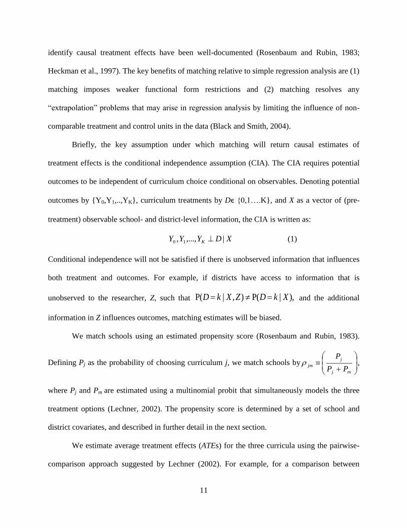
Briefly, the key assumption under which matching will return causal estimates of
treatment effects is the conditional independence assumption (CIA). The CIA requires potential
outcomes to be independent of curriculum choice conditional on observables. Denoting potential
outcomes by {Y0,Y1,..,YK}, curriculum treatments by Dє {0,1….K}, and X as a vector of (pre-
treatment) observable school- and district-level information, the CIA is written as:
XDYYY K |,...,, 10 (1)
Conditional independence will not be satisfied if there is unobserved information that influences
both treatment and outcomes. For example, if districts have access to information that is
unobserved to the researcher, Z, such that P( | , ) P( | ),D k X Z D k X and the additional
information in Z influences outcomes, matching estimates will be biased.
We match schools using an estimated propensity score (Rosenbaum and Rubin, 1983).
Defining Pj as the probability of choosing curriculum j, we match schools by
mj
j
jmPP
P ,
where Pj and Pm are estimated using a multinomial probit that simultaneously models the three
treatment options (Lechner, 2002). The propensity score is determined by a set of school and
district covariates, and described in further detail in the next section.
We estimate average treatment effects (ATEs) for the three curricula using the pairwise-
comparison approach suggested by Lechner (2002). For example, for a comparison between
12
curricula j and m, where Yj and Ym are outcomes for treated and control schools, respectively, we
estimate }),{|(, mjDYYEATE mjmj . We use kernel and local-linear-regression matching
estimators (with the Epanechnikov kernel), which construct the match for each “treated” school
using a weighted average of “control” schools, and vice versa. Prior research suggests that kernel
matching should perform well in our context (Frölich, 2004).16
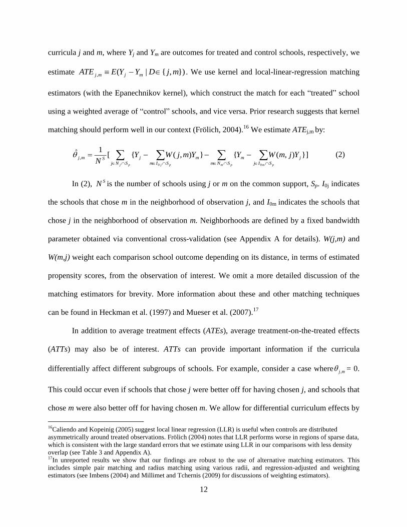
We estimate ATEj,m by:
pm pmpj pj SNm SIj
jm
SNj SIm
mjSmj YjmWYYmjWYN
00
}]),({}),({[1ˆ
, (2)
In (2), SN is the number of schools using j or m on the common support, Sp. I0j indicates
the schools that chose m in the neighborhood of observation j, and I0m indicates the schools that
chose j in the neighborhood of observation m. Neighborhoods are defined by a fixed bandwidth
parameter obtained via conventional cross-validation (see Appendix A for details). W(j,m) and
W(m,j) weight each comparison school outcome depending on its distance, in terms of estimated
propensity scores, from the observation of interest. We omit a more detailed discussion of the
matching estimators for brevity. More information about these and other matching techniques
can be found in Heckman et al. (1997) and Mueser et al. (2007).17
In addition to average treatment effects (ATEs), average treatment-on-the-treated effects
(ATTs) may also be of interest. ATTs can provide important information if the curricula
differentially affect different subgroups of schools. For example, consider a case where ,j m = 0.
This could occur even if schools that chose j were better off for having chosen j, and schools that
chose m were also better off for having chosen m. We allow for differential curriculum effects by
16
Caliendo and Kopeinig (2005) suggest local linear regression (LLR) is useful when controls are distributed
asymmetrically around treated observations. Frölich (2004) notes that LLR performs worse in regions of sparse data,
which is consistent with the large standard errors that we estimate using LLR in our comparisons with less density
overlap (see Table 3 and Appendix A). 17
In unreported results we show that our findings are robust to the use of alternative matching estimators. This
includes simple pair matching and radius matching using various radii, and regression-adjusted and weighting
estimators (see Imbens (2004) and Millimet and Tchernis (2009) for discussions of weighting estimators).
13
estimating ATTs for all of the comparisons in both directions (i.e. ATTj,m and ATTm,j). We briefly
discuss our findings in Section VI, but in general we gain little additional insight from the ATTs.
Finally, it is important to emphasize what a “curriculum effect” means in the context of
our study. Of course, differences in content, pedagogy and presentation will be reflected in our
estimates; but so will other systematic differences in implementation across curricula. For
example, if one curriculum is more amenable to teacher implementation, say by offering a more
detailed teaching guide or providing more publisher support, our estimates will reflect this
difference. As another example, Agodini et al. (2010) report that the average teacher using
SFAW spends 4.8 hours per week on mathematics instruction, whereas for Saxon the average
teacher spends 6.1 hours. Our estimates will capture differences along these lines as well.
One way to describe our estimates is that they capture the “total treatment effects” of the
curricula on mathematics instruction. In many circumstances this is desirable, but in some cases
it may not be. For example, if more time on math instruction reduces time for other subjects then
there could be adverse consequences that would be missed by our estimates. In practice, we find
little evidence to suggest that there are spillover effects, at least on reading scores, but
conceptually it is important to recognize that our estimates will embody all of the systematic
differences in math instruction that come with the adoption of one of these curricula.
Are Schools an Appropriate Unit of Analysis?
We perform our analysis at the school level throughout, despite the fact that the official
curriculum orders come from districts. There are several benefits to our school-level approach
over the district-level alternative. First, the sample of schools is much larger than the sample of
districts. Matching is often described as a “data hungry” procedure, and a key benefit of the
larger sample of schools is that it facilitates better matches (Zhao, 2004). An analogous district
14
level analysis could be performed in principle, and in fact we do verify our findings are
qualitatively similar if we match at the district level instead, but the school-level approach should
result in higher quality matches and is conceptually preferred for this reason.
Second, the CIA requires that we condition on all of the factors that determine curriculum
selection and outcomes. As discussed above, the curriculum-selection process is complicated –
the fact that districts mechanically place the orders does not mean that schools are not involved
in the process. Performing our analysis at the school level allows us to directly control for school
and district-specific features, whereas it is not possible to do the reverse – for example, when we
match districts it is not straightforward to control for disaggregated characteristics of schools.
Third, it is conceptually plausible that administrators focus on raising school-level
achievement. Clearly, school-level administrators will have this focus, but district-level
administrators may also evaluate district performance on a building-by-building basis. If nothing
else, our focus on school-level performance is consistent with recent accountability targets at all
levels (local, state, federal).18
Noting these benefits of the school-level approach, it is still important to acknowledge the
role that districts play in the adoption process. Our matching procedure accounts for this role by
matching schools in terms of district similarity as well (see Section V). In addition, the fact that
schools within a district all move together creates a clustering structure in the data that cannot be
ignored. Accordingly, we cluster our standard errors at the district level throughout the analysis.
The school-level data are the most disaggregated data available in Indiana, and for the
above reasons, we argue that schools are the best units of analysis for our study. Still, the school-
level variables are aggregated up from individual students, and the issue of aggregation bias
18
Federal legislation like NCLB is targeted at the school level. But even in other areas, like teacher accountability,
recent work points to the use of school-level performance measures as being desirable (Ahn and Vigdor, 2011).
15
merits attention. We test for the importance of aggregation bias in our study indirectly using the
falsification exercise in Section VII. There we show that our findings are not driven by
aggregation bias.19
A related and more general issue is in regard to cross-level inference about
the efficacy of educational interventions (Burstein, 1980). In our study the key concern is that
curriculum effects may be different at different levels of analysis. For example, it would be
inadvisable to use our estimates to gain inference about student-level curriculum effects. As a
practical matter our main findings can be replicated if we aggregate up to the district level, but
the same may not occur if we could disaggregate down to the student level (although it is not
clear that student level inference would be conceptually desirable for curriculum interventions).20
V. The Propensity Score
Specification
We use a multinomial probit (MNP) to estimate the propensity scores for schools based
on pre-adoption characteristics. Noting that the curricula of interest were first used in schools in
the fall of 1998, the MNP includes information from the 1996-1997 and 1997-1998 school years.
At the school level we include controls for enrollment, demographics (race, free lunch status,
language status) and outcomes (grade-3 test scores in math and language arts, and attendance)
from 1996-1997, and analogous controls for enrollment and demographics from 1997-1998. At
the district level we include enrollment, outcome and finance controls from 1996-1997, and
enrollment and finance controls from 1997-1998. We also use district-level zip codes to assign
19
Hanushek et al. (1996) show that aggregation leads to upward bias in the estimated effects of educational
interventions in multi-state studies where state information is omitted. Within state, the effect of aggregation bias is
ambiguous. 20
There is a large literature that discusses how inference can be confounded across levels of aggregation in
educational research (for example, see Burstein, 1980; Hanushek et al., 1996; Raudenbush and Bryk, 1986;
Raudenbush, 1988). To illustrate the potential problems with cross-level inference in the present study, consider a
comparison between student-level and school-level curriculum effects. Hypothetically, one could imagine estimating
the student-level effect of SBG from a classroom where students used different curricula. The student-level effect
may be different than the school- or classroom-level effect because SBG involves group work. Because curricula are
group-level interventions, student-level curriculum effects seem conceptually unappealing.
16
year-2000 Census measures of local-area socioeconomic status to each school; namely, median
household income and the share of adults without a high-school diploma. We treat these
variables as fixed-area characteristics. The list of covariates from the MNP is shown in Table 1.
The propensity score model was constructed to include the relevant information available
to schools and districts at the time of the adoption. For instance, we control for 1996-97 school
and district test scores to account for pre-treatment differences in achievement. But because the
adoption decision was made by the summer of 1998, it is unlikely that decision makers had
access to spring 1998 test scores and consequently we do not include these scores in the model
(similarly, we omit annual attendance from 1997-1998). The model also reflects the variety of
potential actors involved in the adoption process. In addition to including school- and district-
level controls, for example, the Census controls are included in acknowledgement of the role of
the local community can play in the adoption process (see Section II).
Although it is impossible to verify that the matching procedure includes all relevant
factors, two pieces of evidence suggest that matching performs reasonably well. First, our
findings are not qualitatively sensitive to reasonable adjustments to the MNP, including the
addition of the 1997-1998 outcome variables, or the addition of more years of lagged test scores.
Second, we perform falsification tests where we estimate curriculum “effects” for students who
were not actually exposed to the curricula (see Section VII). If unobserved factors that are
otherwise unaccounted for in our models are driving our findings, we would anticipate
estimating non-zero curriculum “effects” for the cohorts of unexposed students. The falsification
tests provide no evidence to suggest that our primary estimates are biased by unobservables.
Balancing
In each comparison we match treated and control schools based on the pairwise
propensity scores, and test for covariate balance. Balancing tests are motivated by Rosenbaum
and Rubin (1983), and determine whether )|(| XKDPDX , a necessary condition if the
17
propensity score is to be used to match schools.21
Although achieving covariate balance is
important for any matching analysis that relies on a propensity score, there is no clearly preferred
test for balance. Furthermore, in some cases different balancing tests return different results
(Smith and Todd, 2005). Given this limitation we consider two different tests. The first is a
regression-based test suggested by Smith and Todd (2005) that we perform separately for each
pairwise comparison and for each covariate in each year. In the comparison between curricula j
and m we estimate:
4
9
3
8
2
765
4
4
3
3
2
210
******* jmjmjmjm
jmjmjmjmk
DDDDD
X (3)
In (3), Xk represents a covariate from the propensity-score specification, jm is the estimated
pairwise propensity score, and D indicates treatment. We test whether the coefficients 5 9- are
jointly equal to zero in each regression – that is, we test whether treatment predicts the X’s
conditional on a quartic of the propensity score.
The second test measures the absolute standardized difference in observables after
matching, and was originally suggested by Rosenbaum and Rubin (1985). The formula for the
absolute standardized difference for covariate Xk is given by:
0 0
1| [ { ( , ) } { ( , ) }] |
( ) *100( ) ( )
2
j p j p m p m p
kj km km kjSj N S m I S m N S j I S
k
kj km
X W j m X X W m j XN
SDIFF XVar X Var X
(4)
The numerator in (4) is analogous to the formula for our matching estimators in (2) where we
replace Y with Xk and take the absolute value (note the denominator is calculated using the full
21
The MNP results are omitted for brevity but available upon request. To provide a sense of the predictive power of
the covariates we estimate separate linear-regression models for each curriculum comparison. The dependent
variable indicates the adoption of one of the curricula, and the independent variables are the covariates from the
MNP. Within comparison pairs, the covariates explain 23 to 42 percent of the variability in curriculum adoptions.
18
sample). A weakness of using standardized differences is that there is not a clear rule by which to
judge the results, although Rosenbaum and Rubin (1985) suggest that a value of 20 is large.
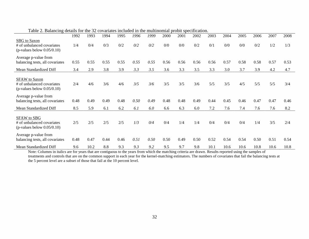
Our MNP uses 32 school- and district-level covariates. Table 2 reports summary results
from the balancing tests by comparison and year. From the regression tests we report the number
of covariates where the F-test rejects the null hypothesis at the 5- or 10-percent level, and the
average p-value across all F-tests. We also report the average absolute standardized difference
across all covariates.22
Table 2 shows that our comparison between SBG and Saxon is
particularly well-balanced. For our other comparisons the covariates are less balanced, although
it is not clear that the levels of imbalance are cause for concern. For example, although the
average absolute standardized difference is larger in the comparisons involving SFAW,
compared to other methodologically-similar studies the averages in Table 2 are quite reasonable.
We also calculate the divergence between the densities of the estimated propensity scores
for treated and control units. Intuitively, density divergence will affect the precision of the
estimates, and can be generally informative about the extent to which the data environment is
favorable for matching (the key issue being overlap in the distributions of observables). Similarly
to the balancing tests, our analysis of density divergence suggests that the data conditions are
most favorable in our comparison of SBG and Saxon. See Appendix A for details.
VI. Results
Table 3 presents the estimated curriculum effects for all grade-3 cohorts who were ever
exposed to the curricula of interest. Each cohort is labeled according to the year of its spring test
(e.g., the 1998-1999 cohort is labeled “1999”). All of the estimates are standardized using the
22
These reporting measures are somewhat standard in the literature (e.g., see Smith and Todd, 2005; Sianesi, 2004),
but in summarizing the information some details are lost. Appendix Table B.1 reports balancing results for all 32
covariates in each comparison for a single year of our data (2002) to illustrate covariate balance more fully.
19
distribution of student-level test scores.23
In addition to the matching estimators, we also report
OLS estimates where we regress test score outcomes on the covariates used in the propensity
score model and indicator variables for curriculum adoptions, retaining the pairwise
comparisons. The standard errors for the matching and OLS estimates are clustered at the district
level and the matching-estimator standard errors are bootstrapped with 250 repetitions.24
Focusing first on our largest comparison between SBG and Saxon, and the estimates for
the fully-exposed cohorts (2001-2004), we find that SBG meaningfully outperformed Saxon. By
averaging the kernel-matching estimates across these cohorts we estimate that among the sample
of schools that chose SBG or Saxon, the average effect of using SBG was roughly 0.13 standard
deviations of the test. Our estimates are also consistent with SFAW outperforming Saxon. There
we estimate an average effect of 0.06 standard deviations, although only two of the four
estimates are statistically significant and the estimate from 2004 is particularly small. Our results
also suggest, at least weakly, that SBG outperformed SFAW, although the estimates are noisy
enough that we cannot draw strong inference from this latter comparison.
We also briefly consider the possibility that treatment effects depend on treatment status.
In unreported results we estimate ATTs for each comparison and in each direction. In our
comparison between SBG and Saxon the treatment effects do not depend on treatment status, and
similarly for our comparison between SFAW and SBG (although again, these estimates are
noisy). Only in our comparison between SFAW and Saxon do we find any evidence of
differential effects – Saxon appears to perform less poorly relative to SFAW at schools that
actually chose Saxon. Nonetheless, even our estimates of ATTSaxon,SFAW suggest that schools that
23
Our outcome data are reported at the building level. Appendix Table C.2 shows how we scale our estimates so
that they are in the metric of the student-level distribution of scores. 24
We obtain the optimal number of bootstrap repetitions following Ham et al. (2006). We re-sample entire districts.
Abadie and Imbens (2006) show that bootstrapping cannot be used to obtain standard errors for nearest-neighbor
matching estimators, but their result does not apply to smoother estimators like those used here.
20
chose Saxon would have been better off had they instead chosen SFAW.
The magnitudes of the curriculum effects are economically meaningful, particularly when
weighed against the marginal costs of choosing one curriculum over another. For instance, Fryer
and Levitt (2006) show that between grades one and three, the black-white achievement gap
grows at a rate of approximately 0.10 standard deviations per year. Contrasting this estimate with
the results from our most-compelling comparison suggests that choosing SBG over Saxon has an
effect that is equivalent to roughly one year’s worth of expansion of the black-white achievement
gap.25
Given that curricula tend to be similarly priced (the texts from Saxon, SBG, and SFAW,
were, averaged over grades 1-3, $23.08, $24.80 and $25.34, respectively), selecting a better
curriculum appears to be a cost-effective way to improve student achievement.26
Next we turn to the partially-exposed cohorts. One common theme is that the point
estimates for the 2005 and 2006 cohorts are generally larger than for the 1999 and 2000 cohorts.
An explanation is that there are familiarity issues related to curriculum implementation. For
example, students who used the curricula when the curricula were first introduced may have had
a different experience than the students who used the curricula toward the end of the adoption
cycle.27
The curricula of may also have had legacy effects on instruction, which would have
affected the 2005 and 2006 cohorts even as they transitioned out of the adoption cycle.
An issue with interpreting the estimates from the partially exposed cohorts is that these
students were also exposed to other curricula in other adoption cycles, and this may attenuate the
25
Fryer and Levitt (2006) analyze a different testing instrument; however, similar estimates of the black-white
achievement gap spread are available elsewhere (see, for example, Chubb and Loveless, 2002). 26
Certainly the short-term achievement effects are notable, but a qualification is that we do not know whether
curriculum effects persist over time. Recent evidence in other contexts raises concerns about the general persistence
of educational interventions (e.g., Jacob et al., 2008; U.S. Department of Health and Human Services, 2010). Earlier
versions of this work attempted to evaluate the persistence of curriculum effects; however, there are too many
potentially confounding factors to draw conclusions from the Indiana data. This is an area for future research. 27
We cannot directly test for familiarity effects among the partially exposed cohorts because differences in
familiarity as the curricula are phased in are confounded by differences in exposure by cohort.
21
estimates. The degree of attenuation will depend on the extent to which curriculum quality is
correlated across adoption cycles for treatment and control schools. We explore this issue to the
extent possible in Table 4, where we compare curriculum adoptions for grades 1-3 in the 2004
adoption cycle across uniform adopters from 1998 (we do not observe math curriculum
adoptions prior to 1998, therefore we cannot examine across-cycle adoptions in earlier periods).
Table 4 shows adoption shares in 2004 for the four most popular curricula from that
adoption cycle. Saxon adopters in 1998 were much more likely to adopt Saxon in 2004, but
adopters of the other two curricula are dispersed across alternative options. Without knowing the
respective qualities of the different curricula adopted outside of the 1998 adoption cycle it is
difficult to form expectations based on the patterns in Table 4. Ultimately, given the potential for
attenuation in the estimates for the partially exposed cohorts, and the sizes of our standard errors,
we cannot make strong inference about partial-exposure curriculum effects.
Another interesting aspect of Table 4 is that it shows the changing market shares of
curriculum publishers over time in Indiana. Saxon, despite its relative underperformance in our
analysis, maintained its near-50-percent market share in 2004. Although we found SBG was the
most effective curriculum during the 1998 adoption cycle, it did not appear in 2004. The
publisher of SBG was bought by Pearson Publishing, and Pearson phased out SBG in favor of
SFAW, which it also publishes. SFAW’s market share fell from roughly fifteen to nine percent.
Overall, our most reliable estimates come from the four fully-exposed cohorts. In our
most compelling comparison, we find that SBG outperformed Saxon by a substantial margin.
Both of these curricula share the same basic pedagogical approach (traditional). With researchers
and policymakers placing so much emphasis on differences between the traditional and reform
pedagogies, our findings serve as a reminder that other differences should not be overlooked.
22
Our analysis also suggests that SFAW somewhat outperformed Saxon; and if anything, SBG
outperformed SFAW, although inference from the latter comparison is clouded by statistical
imprecision. Finally, we show that Saxon’s market share did not diminish in the next adoption
cycle despite our finding of relative underperformance during the 1998 cycle. One explanation is
that educational administrators do not have reliable evidence on curricular effectiveness.28
VII. Falsification Tests
Matching estimators will not return causal estimates if conditional independence is
violated, and there are a number of ways that this could occur in our study. For example, there
could be systematic differences in teacher or administrator quality across different curriculum
adopters. If these differences are correlated with the curriculum adoptions and student
achievement, but poorly proxied for by the controls in the propensity-score model, they could
introduce bias. Or, if there are differences across adopters with respect to mathematics
instruction – perhaps in districts’ general commitments to mathematics – that are not driven by
the curricula themselves, this could bias our estimates. A third possibility is that curriculum
adoptions in other subjects (like reading) may be correlated with math adoptions and math
achievement.29
Any of these factors, or many others, could potentially bias our findings.
While it is impossible to exhaustively consider all possible sources of bias, we provide
evidence about the general reliability of our findings using two types of falsification tests. First,
we estimate curriculum effects on test scores for cohorts of students who never used the curricula
of interest. The logic of these tests can be illustrated with an example. Suppose that there are
28
We cannot rule out that Saxon does not perform better on tests in different grades. We base our conclusion on our
findings for grade-3 achievement during this particular adoption cycle. That said, it is likely that grade-3 was closely
tracked by school administrators during our data panel since grade-3 was the only tested grade in most elementary
schools prior to NCLB. In Section VIII we discuss how our results may not extend to other contexts-such as in
settings where the student population differs from the student population in Indiana. 29
In fact, we directly tested for this particular possibility by estimating the correlations between reading adoptions
and math achievement (non-zero correlations are a prerequisite if reading adoptions are to be a relevant omitted
variable). Even unconditionally, reading adoptions do not predict math achievement.
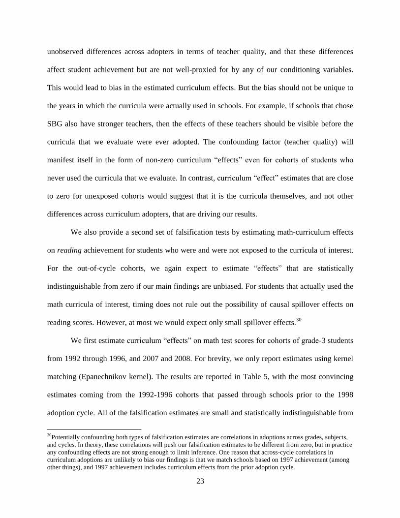
23
unobserved differences across adopters in terms of teacher quality, and that these differences
affect student achievement but are not well-proxied for by any of our conditioning variables.
This would lead to bias in the estimated curriculum effects. But the bias should not be unique to
the years in which the curricula were actually used in schools. For example, if schools that chose
SBG also have stronger teachers, then the effects of these teachers should be visible before the
curricula that we evaluate were ever adopted. The confounding factor (teacher quality) will
manifest itself in the form of non-zero curriculum “effects” even for cohorts of students who
never used the curricula that we evaluate. In contrast, curriculum “effect” estimates that are close
to zero for unexposed cohorts would suggest that it is the curricula themselves, and not other
differences across curriculum adopters, that are driving our results.
We also provide a second set of falsification tests by estimating math-curriculum effects
on reading achievement for students who were and were not exposed to the curricula of interest.
For the out-of-cycle cohorts, we again expect to estimate “effects” that are statistically
indistinguishable from zero if our main findings are unbiased. For students that actually used the
math curricula of interest, timing does not rule out the possibility of causal spillover effects on
reading scores. However, at most we would expect only small spillover effects.30
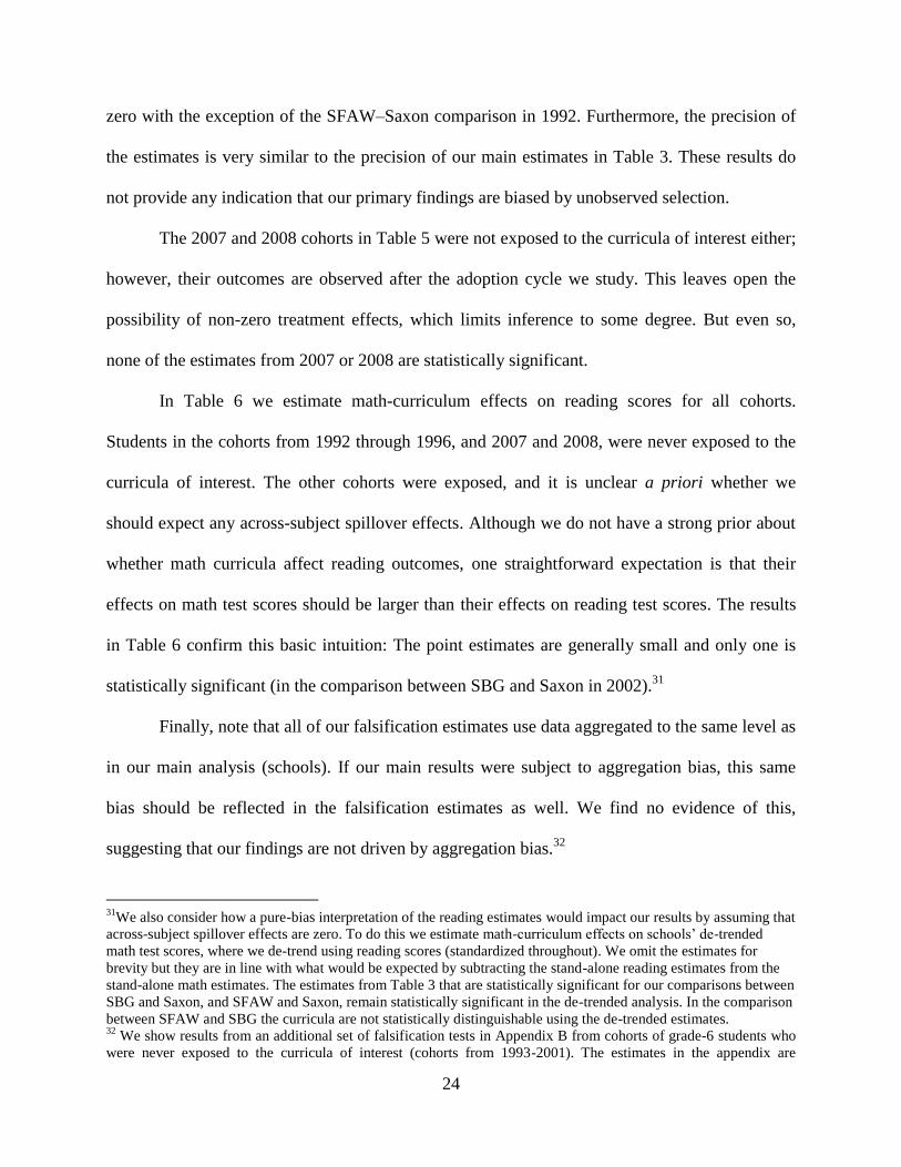
We first estimate curriculum “effects” on math test scores for cohorts of grade-3 students
from 1992 through 1996, and 2007 and 2008. For brevity, we only report estimates using kernel
matching (Epanechnikov kernel). The results are reported in Table 5, with the most convincing
estimates coming from the 1992-1996 cohorts that passed through schools prior to the 1998
adoption cycle. All of the falsification estimates are small and statistically indistinguishable from
30
Potentially confounding both types of falsification estimates are correlations in adoptions across grades, subjects,
and cycles. In theory, these correlations will push our falsification estimates to be different from zero, but in practice
any confounding effects are not strong enough to limit inference. One reason that across-cycle correlations in
curriculum adoptions are unlikely to bias our findings is that we match schools based on 1997 achievement (among
other things), and 1997 achievement includes curriculum effects from the prior adoption cycle.
24
zero with the exception of the SFAW–Saxon comparison in 1992. Furthermore, the precision of
the estimates is very similar to the precision of our main estimates in Table 3. These results do
not provide any indication that our primary findings are biased by unobserved selection.
The 2007 and 2008 cohorts in Table 5 were not exposed to the curricula of interest either;
however, their outcomes are observed after the adoption cycle we study. This leaves open the
possibility of non-zero treatment effects, which limits inference to some degree. But even so,
none of the estimates from 2007 or 2008 are statistically significant.
In Table 6 we estimate math-curriculum effects on reading scores for all cohorts.
Students in the cohorts from 1992 through 1996, and 2007 and 2008, were never exposed to the
curricula of interest. The other cohorts were exposed, and it is unclear a priori whether we
should expect any across-subject spillover effects. Although we do not have a strong prior about
whether math curricula affect reading outcomes, one straightforward expectation is that their
effects on math test scores should be larger than their effects on reading test scores. The results
in Table 6 confirm this basic intuition: The point estimates are generally small and only one is
statistically significant (in the comparison between SBG and Saxon in 2002).31
Finally, note that all of our falsification estimates use data aggregated to the same level as
in our main analysis (schools). If our main results were subject to aggregation bias, this same
bias should be reflected in the falsification estimates as well. We find no evidence of this,
suggesting that our findings are not driven by aggregation bias.32
31
We also consider how a pure-bias interpretation of the reading estimates would impact our results by assuming that
across-subject spillover effects are zero. To do this we estimate math-curriculum effects on schools’ de-trended
math test scores, where we de-trend using reading scores (standardized throughout). We omit the estimates for
brevity but they are in line with what would be expected by subtracting the stand-alone reading estimates from the
stand-alone math estimates. The estimates from Table 3 that are statistically significant for our comparisons between
SBG and Saxon, and SFAW and Saxon, remain statistically significant in the de-trended analysis. In the comparison
between SFAW and SBG the curricula are not statistically distinguishable using the de-trended estimates. 32
We show results from an additional set of falsification tests in Appendix B from cohorts of grade-6 students who
were never exposed to the curricula of interest (cohorts from 1993-2001). The estimates in the appendix are
25
VIII. Conclusion
We use a unique administrative data panel from Indiana to compare the effectiveness of
three elementary-mathematics curricula. We measure curriculum effects using test scores on the
Indiana state test (the ISTEP). Our results indicate that there are substantial differences in
effectiveness across the three curricula, and in particular, between the two curricula that held the
largest market shares in the state during our study.
Our research makes two contributions to the literature. First, we show that important
differences in curricular effectiveness can exist between curricula that share the same
pedagogical approach. Specifically, we find that during the 1998-2004 adoption cycle in Indiana,
the Silver Burdett Ginn curriculum meaningfully outperformed the Saxon curriculum, and both
curricula are best-characterized as traditional in pedagogy. This suggests that other differences
between these curricula, and other curricula more generally, are important determinants of
achievement and merit attention from researchers and policymakers.
Our study also provides a template for how similar studies in other states could be
performed. The thinness of the empirical literature on curricular effectiveness is striking, and the
most prominent obstacle in the way of producing more studies is the lack of data. Currently,
Indiana is one of only two states of which we are aware that collects and makes curriculum-
adoption information available, and many states do not collect data at all. Such data would be
cheap and easy to collect, particularly compared to other data elements in many state
longitudinal systems, and could be used to learn much about this important educational resource.
One advantage of having more studies on curricular effectiveness is that they can be used
to examine how different curricula perform in different contexts. Unlike some other educational
qualitatively consistent with the other falsification findings.
26
interventions, curricula are used by virtually all students in all schools. This implies considerable
heterogeneity in the contexts in which curricula are used; both in terms of the actors involved
(students and teachers), and potentially the objectives of the intervention (e.g., differences in
standards across states or school districts). The right curriculum in one circumstance may not be
right in another. As a specific example, Agodini et al. (2010) find that Saxon outperforms
SFAW, while our findings suggest the opposite (weakly). An important contextual difference is
that Agodini et al. analyze schools where students are significantly more disadvantaged than
students in the typical Indiana school.33
It may be inadvisable for a disadvantaged school district
to choose SFAW (or perhaps SBG) based on our study, or alternatively, for an advantaged
district to choose Saxon based on the Agodini et al. study.34
But both studies provide valuable
information for administrators in the right context. More generally, the current sparseness of the
literature makes it difficult for educational administrators to make informed curriculum-adoption
decisions. But if the literature were expanded, patterns would emerge across multiple studies that
would allow us to determine which curricula are most effective in which circumstances.35
33
The average share of students on free/reduced-price lunch in the schools in Agodini et al. (2010) is 50 percent; in
our study it is 27 percent. Schools in their study are, on average, 38.5 percent white; in our study the white share is
over 90 percent. Also, they find that Saxon outperforms SFAW in grade-2; our findings are for grade-3. 34
We attempted to directly examine the role of student disadvantage as a cause of the discrepancy in findings across
studies, but could not construct a large enough sample of Indiana schools that matched the level of disadvantage in
the Agodini et al. (2010) study. Based on what we could ascertain from our supplementary analysis, however,
differences in student disadvantage appear to explain some of discrepancy between studies. This hypothesis is
further supported by comparing the findings in wave-1 and wave-2 of the Agodini et al. study. The sample of
schools in wave-1 of the experiment was more disadvantaged than the sample in wave-2, and the differences that
they document between Saxon and SFAW are smaller in the second wave (and significant only in grade-2). 35
Virtually every study has contextual features that limit external validity to some degree (see Schoenfeld (2006) for
a general discussion of contextual issues in curriculum evaluation). The two most prominent Indiana-specific
features in our analysis are the students and the test. We would expect our findings to carry over well for states that
use tests similar to the ISTEP, but perhaps not elsewhere. And our findings may not extrapolate well to states or
regions where the population differs greatly from Indiana, which is a fairly rural state and, as noted in the text,
relatively advantaged (relative to both the Agodini et al. sample and the nation as a whole). A third issue is that our
analysis is based entirely on grade-3 test scores and it is not clear how our results would replicate in other grades.
All of these issues point back to the larger problem that the literature on curricular effectiveness is so thin – more
studies from more states and more grades would be greatly informative.

27
References
Abadie, Alberto and Guido W. Imbens. 2006. On the Failure of the Bootstrap for Matching
Estimators. NBER Technical Working Paper No. 325.
Agodini, Robert and Barbara Harris and Sally Atkins-Burnett and Sheila Heaviside, and Timothy
Novak. 2010. Achievement Effects of Four Early Elementary School Math Curricula: Findings
for First and Second Graders. National Center for Education Evaluation and Regional
Assistance, U.S. Department of Education, Institute of Education Sciences. NCEE 2011-4001.
Agodini, Robert and Barbara Harris and Sally Atkins-Burnett and Sheila Heaviside, and Timothy
Novak. 2009. Achievement Effects of Four Early Elementary School Math Curricula: Findings
From First Graders in 39 Schools. National Center for Education Evaluation and Regional
Assistance, U.S. Department of Education, Institute of Education Sciences. NCEE 2009-4052.
Ahn, Thomas and Jacob L. Vigdor. 2011. Making Teacher Incentives Work. Education Outlook
No. 5, American Enterprise Institute for Public Policy Research.
An, Shuhua. 2004. The Middle Path in Math Instruction: Solutions for Improving Math
Education. Scarecrow Education. Oxford, U.K.
Association of American Publishers. 2001. Less than a Penny: The Instructional Materials
Shortage & How It Shortchanges Students, Teachers, & Schools. Association of American
Publishers Report.
Ballou, Dale. 1996. "Do Public Schools Hire the Best Applicants?” Quarterly Journal of
Economics 111(1), pp. 97-133.
Black, Dan and Jeffrey Smith. 2004. “How Robust is the Evidence on the Effects of College
Quality? Evidence From Matching,” Journal of Econometrics 121 (2), 99-124.
Bloom, K.C. and Shuell, T.J. 1981.Effects of massed and distributive practice on the learning
and retention of second-language vocabulary. Journal of Education Research, 74, 245-248.
Bolser, S., and D. Gilman. 2003. Saxon Math, Southeast Fountain Elementary School: Effective
or ineffective? (ERIC Document Reproduction Service No. ED474537).
Borman, Geoffrey D. and N. Maritza Dowling and Carrie Schneck. 2008. “A Multisite Cluster
Randomized Field Trial of Open Court Reading,” Educational Evaluation and Policy Analysis
30 (4), 389-407.
Braswell, James S. and Anthony D. Lutkus and Wendy S. Grigg and Shari L. Santapau and
Brenda Tay-Lim and Matthew Johnons. 2001. “The Nation’s Report Card: Mathematics 2000”,
U.S. Department of Education: Office of Educational Research and Improvement.
Burstein, Leigh. 1980. “The Analysis of Multilevel Data in Educational Research and
Evaluation,”Review of Research in Education, Vol. 8, 158-233.
28
Caliendo, Marco and Sabine Kopeinig. 2005. “Some Practical Guidance for the Implementation
of Propensity Score Matching,” IZA Discussion Paper No. 1588.
Chubb, John and Tom Loveless. 2002. Bridging the Achievement Gap, Brookings Institution
Press, Washington, D.C.
Educational Marketer. 1998a. “Addison Wesley Longman’s Earnings Improve in the First Half
Of 1998.” August 10, 1998.
-- 1998b. “Addison Wesley Longman Rebounds To Take Louisiana's $25 Million K-12
Math Adoption.” September 14, 1998.
--1999a. “A $250M Allocation For K-8 Math Materials Has Publishers Looking to
California For Big Sales.” June 21, 1999.
-- 1999b.“Two Big Wins Help Pearson Take First Place in EM’s Adoption Scorecard For
1999.” December 20, 1999.
Ellis, Rod. 2006. “Current Issues in the Teaching of Grammar: An SLA Perspective”. TESOL
Quarterly, 40 (1).
Finn, Chester. 2004. “The Mad, Mad World of Textbook Adoption” The Thomas B Fordham
Foundation and Institute Report. Washington, D.C.
Freeman, Donald J. and Andrew C. Porter. 1989. “Do Textbooks Dictate the Content of
Mathematics Instruction in Elementary Schools?” American Educational Research Journal 26
(3) pp. 403-421.
Frölich, Markus. 2004. “Finite-Sample Properties of Propensity-Score Matching and Weighting
Estimators,” The Review of Economics and Statistics 86 (1), 77-90.
Fryer, Roland and Steven Levitt. 2006. “The Black-White Test Score Gap Through Third
Grade,” American Law and Economics Review 8 (2), 249-281.
Ham, John and Xianghong Li and Patricia Reagan. 2006. “Propensity Score Matching, a
Distance-Based Measure of Migration, and the Wage Growth of Young Men,” Federal Reserve
Bank, Staff Report No. 212.
Hanushek, Eric and Steven Rivkin and Lori Taylor. 1996. “Aggregation and the Estimated
Effects of School Resources” Review of Economics and Statistics 78 (4) 611-627.
Heckman, James and Hidehiko Ichimura, and Petra Todd. 1997. “Matching as an Econometric
Evaluation Estimator: Evidence from Evaluating a Job-Training Programme,” Review of
Economic Studies 64 (4), 261-294.
Houghton Mifflin Harcourt Publishers (HMHP). 2008. Saxon Math Response to the National
29
Math Advisory Panel Report. Accessed online at:
http://www.hmheducation.com/saxonmathaga/pdf/topics/nmap_response.pdf
Imbens, Guido. 2004. “Nonparametric Estimation of Average Treatment Effects Under
Exogeneity: A Review,” The Review of Economics and Statistics 86 (1), 4-29.
Jacob, Brian and Lars Lefgren and David Sims. 2008. “The Persistence of Teacher-Induced
Learning Gains,” NBER Working Paper No. 14065.
Kullback, Solomon and Richard Leibler. 1951. “On Information and Sufficiency,” Annals of
Mathematical Statistics 22 (1), 79-86.
Lechner, Michael. 2002. “Program Heterogeneity and Propensity Score Matching: An
Application to the Evaluation of Active Labor Market Policies,” The Review of Economics and
Statistics 84 (2), 205-220.
Mayer, R.E. (2001). Multimedia learning. New York: Cambridge University Press.
Mayer, R.E., and Moreno, R. 1998. A split-attention effect in multimedia learning: Evidence for
dual-processing systems in working memory. Journal of Educational Psychology, 90, 312–20.
Millimet, Daniel L. and Rusty Tchernis. 2009. “On the Specification of Propensity Scores, with
Applications to the Analysis of Trade Policies,” Journal of Business & Economic Statistics 27
(3), 397-415.
Mueser, Peter R. and Kenneth R. Troske and Alexey Gorislavsky.2007. “Using State
Administrative Data to Measure Program Performance,” The Review of Economics and Statistics
89 (4), 761-83.
National Research Board. 2004. On Evaluating Curricular Effectiveness: Judging the quality of
K-12 Mathematics Evaluations, The National Academies Press, Washington DC.
National Council of Teachers of Mathematics. 2009. “Selecting the Right Curriculum”,
Curriculum Research Brief.
National Mathematics Advisory Panel. 2008. “The Final Report of the National Mathematics
Advisory Panel”, U.S. Department of Education. Accessed online at:
http://www2.ed.gov/about/bdscomm/list/mathpanel/report/final-report.pdf
National Mathematics Advisory Panel. 2007. “Preliminary Report to the President”, U.S.
Department of Education. Accessed online at:
http://www2.ed.gov/about/bdscomm/list/mathpanel/pre-report.pdf
Rea, C.P. and V. Modigliani. 1985. “The Effect of expanded versus massed practice on the
retention of multiplication facts and spelling lists”, Human Learning, 4, 11-18.
30
Resendez, M. and Manley. M.A. 2005. “The relationship between using Saxon Elementary and
Middle School Math and student performance on Georgia Statewide assessments”, Harcourt.
Riordan, Julie E. and Pendred E. Noyce. 2001. The impact of two standards-based mathematics
curricula on student achievement in Massachusetts. Journal for Research in Mathematics
Education32(4), 368–398.
Raudenbush, Stephen W. 1988. Educational Applications of Hierarchical Linear Models: A
Review. Journal of Education Statistics, 13(2), 85-116.
Raudenbush, Stephen W. and Anthony S. Bryk. 1986. A Hierarchical Model for Studying School
Effects. Sociology of Education, 59(1), 1-17.
Rosenbaum, Paul R. and Donald B. Rubin. 1983. “The Central Role of the Propensity Score in
Observtional Studies for Causal Effects,” Biometrika 70 (1), 41-55.
Rosenbaum, Paul R. and Donald B. Rubin. 1985. “The Bias due to Incomplete Matching,”
Biometrika 41 (1), 103-116.
Sianesi, Barbara. 2004. An evaluation of the Swedish system of active labor market programs in
the 1990s. Review of Economics and Statistics, 86(1), 133-155.
Schoenfeld, Alan H. (2006). What doesn't work: The challenges and failure of the what works
clearinghouse to conduct meaningful reviews of studies of mathematics curricula. Educational
Researcher, 35(2): 13-21.
Slavin, Robert E. and Cynthia Lake.2008. “Effective Programs in Elementary Mathematics: A
Best-Evidence Synthesis,” Review of Educational Research, 78 (3), 427-515.
Smith, Jeffrey and Petra Todd. 2005. “Rejoinder,” Journal of Econometrics 125 (2), 365-375.
Sweller, John and Graham Cooper. 1985. “The Use of Worked Examples as a Substitute for
Problem Solving in Learning Algebra”, Cognition and Instruction, 2 (1), 59-89.
U.S. Department of Health and Human Services, Administration for Children and Families.
2010. Head Start Impact Study. Final Report. Washington, DC.
Trafton, J.G. and B.J. Reiser. 1993. The contributions of studying examples and solving
problems to skill acquisition. In M. Polson (Ed.), Proceedings of the 15th
Annual Conference of
the Cognitive Science Society, 1017-1022.
What Works Clearinghouse. 2007. Topic Report: Elementary School Math. Available at:
http://ies.ed.gov/ncee/wwc/reports/elementary_math/topic
Zhao, Zhong. 2004. “Using Matching to Estimate Treatment Effects: Data Requirements,
Matching Metrics, and Monte Carlo Evidence” Review of Economics and Statistics, 86, 91-107.
31
Table 1. Average Characteristics of Schools and Districts, by Adopted Curriculum (1997 values)
Sample
Average
Saxon SBG SFAW
School-Level Outcomes
Attendance Rate 96.2 96.3a 96.1
a 96.3
Grade-3 Math Test Score 496.6 496.5 494.2c 499.7
c
Grade-3 Language Test Score 496.7 496.1 495.8 498.7
School-Level Characteristics
Percent Free Lunch 27.4 24.7a,b
28.5a 30.5
b
Percent Reduced Lunch 6.7 7.1a 6.3
a 6.6
Percent Not Fluent in English 1.2 0.7a 1.7
a 1.2
Percent Language Minority 2.6 1.8a 3.9
a 2.6
Percent White 91.3 95.4a,b
88.0a 88.4
b
Percent Black 5.6 2.3a,b
7.2a,c
9.2b,c
Percent Asian 0.7 0.4a,b
0.9a 1.1
b
Percent Hispanic 2.2 1.8a,b
3.7a,c
1.1b,c
Percent American Indian 0.2 0.1 0.2 0.2
Enrollment (log) 5.95 5.92 5.97 5.96
N (Schools) 716 311 221 184
District-Level Outcomes
Attendance Rate 95.8 95.7b 95.8 96.1
b
Grade-3 Math Test Score 498.1 495.8b 498.1
a,c 506.9
b
Grade-3 Language Test Score 498.9 496.5a,b
500.6a 505.6
b
District-Level Characteristics
Enrollment (log) 7.72 7.60a,b
7.8a,c
8.2b,c
Total Per-Pupil Revenue(log) 8.83 8.81b 8.84 8.87
b
Local Per-Pupil Revenue(log) 7.24 7.18b 7.24
c 7.47
b,c
Census Information (District Level)
Median Household Income (logs) 10.81 10.8a,b
10.8a,c
10.9b,c
Share of Population with Low Education 18.2 18.8b 19.2
c 14.3
b,c
N (Districts) 213 124 56 33 a Indicates statistically significant difference at the 10% level between Saxon and SBG adopters.
b Indicates statistically significant difference at the 10% level between Saxon and SFAW adopters.
c Indicates statistically significant difference at the 10% level between SBG and SFAW adopters.
Note: The propensity-score specification also uses italicized information from 1998 – differences in means for these
years are not reported for brevity.
32
Table 2. Balancing details for the 32 covariates included in the multinomial probit specification. 1992 1993 1994 1995 1996 1999 2000 2001 2002 2003 2004 2005 2006 2007 2008
SBG to Saxon
# of unbalanced covariates
(p-values below 0.05/0.10)
1/4 0/4 0/3 0/2 0/2 0/2 0/0 0/0 0/2 0/1 0/0 0/0 0/2 1/2 1/3
Average p-value from
balancing tests, all covariates 0.55 0.55 0.55 0.55 0.55 0.55 0.56 0.56 0.56 0.56 0.57 0.58 0.58 0.57 0.53
Mean Standardized Diff 3.4 2.9 3.8 3.9 3.3 3.5 3.6 3.3 3.5 3.3 3.0 3.7 3.9 4.2 4.7
SFAW to Saxon
# of unbalanced covariates
(p-values below 0.05/0.10)
2/4 4/6 3/6 4/6 3/5 3/6 3/5 3/5 3/6 5/5 3/5 4/5 5/5 5/5 3/4
Average p-value from
balancing tests, all covariates 0.48 0.49 0.49 0.48 0.50 0.49 0.48 0.48 0.49 0.44 0.45 0.46 0.47 0.47 0.46
Mean Standardized Diff 8.5 5.9 6.1 6.2 6.1 6.0 6.6 6.3 6.0 7.2 7.6 7.4 7.6 7.6 8.2
SFAW to SBG
# of unbalanced covariates
(p-values below 0.05/0.10)
2/5 2/5 2/5 2/5 1/3 0/4 0/4 1/4 1/4 0/4 0/4 0/4 1/4 3/5 2/4
Average p-value from
balancing tests, all covariates 0.48 0.47 0.44 0.46 0.51 0.50 0.50 0.49 0.50 0.52 0.54 0.54 0.50 0.51 0.54
Mean Standardized Diff 9.6 10.2 8.8 9.3 9.3 9.2 9.5 9.7 9.8 10.1 10.6 10.6 10.8 10.6 10.8
Note: Columns in italics are for years that are contiguous to the years from which the matching criteria are drawn. Results reported using the samples of
treatments and controls that are on the common support in each year for the kernel-matching estimators. The numbers of covariates that fail the balancing tests at
the 5 percent level are a subset of those that fail at the 10 percent level.
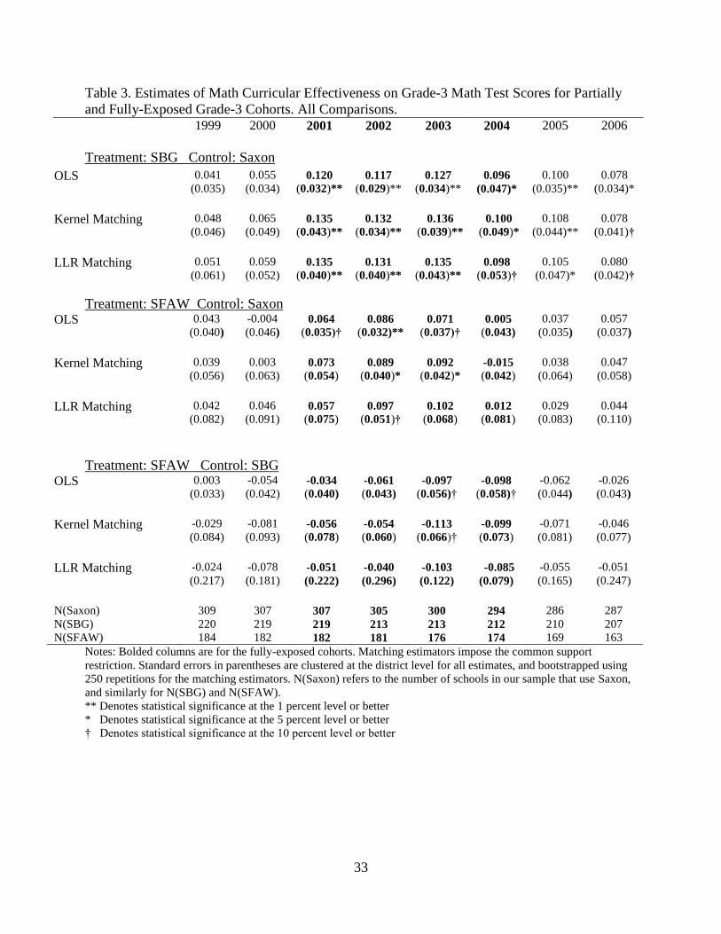
33
Table 3. Estimates of Math Curricular Effectiveness on Grade-3 Math Test Scores for Partially
and Fully-Exposed Grade-3 Cohorts. All Comparisons.
1999 2000 2001 2002 2003 2004 2005 2006
Treatment: SBG Control: Saxon
OLS 0.041
(0.035)
0.055
(0.034) 0.120
(0.032)**
0.117
(0.029)**
0.127
(0.034)**
0.096
(0.047)*
0.100
(0.035)**
0.078
(0.034)*
Kernel Matching 0.048
(0.046)
0.065
(0.049) 0.135
(0.043)**
0.132
(0.034)**
0.136
(0.039)**
0.100
(0.049)*
0.108
(0.044)**
0.078
(0.041)†
LLR Matching 0.051
(0.061)
0.059
(0.052) 0.135
(0.040)**
0.131
(0.040)**
0.135
(0.043)**
0.098
(0.053)†
0.105
(0.047)*
0.080
(0.042)†
Treatment: SFAW Control: Saxon OLS 0.043
(0.040)
-0.004
(0.046) 0.064
(0.035)†
0.086
(0.032)**
0.071
(0.037)†
0.005
(0.043)
0.037
(0.035)
0.057
(0.037)
Kernel Matching 0.039
(0.056)
0.003
(0.063) 0.073
(0.054) 0.089
(0.040)*
0.092
(0.042)*
-0.015
(0.042)
0.038
(0.064)
0.047
(0.058)
LLR Matching 0.042
(0.082)
0.046
(0.091) 0.057
(0.075) 0.097
(0.051)†
0.102
(0.068) 0.012
(0.081)
0.029
(0.083)
0.044
(0.110)
Treatment: SFAW Control: SBG OLS 0.003
(0.033)
-0.054
(0.042) -0.034
(0.040)
-0.061
(0.043)
-0.097
(0.056)†
-0.098
(0.058)†
-0.062
(0.044)
-0.026
(0.043)
Kernel Matching -0.029
(0.084)
-0.081
(0.093) -0.056
(0.078) -0.054
(0.060) -0.113
(0.066)†
-0.099
(0.073)
-0.071
(0.081)
-0.046
(0.077)
LLR Matching -0.024
(0.217)
-0.078
(0.181) -0.051
(0.222)
-0.040
(0.296)
-0.103
(0.122)
-0.085
(0.079)
-0.055
(0.165)
-0.051
(0.247)
N(Saxon) 309 307 307 305 300 294 286 287
N(SBG) 220 219 219 213 213 212 210 207
N(SFAW) 184 182 182 181 176 174 169 163
Notes: Bolded columns are for the fully-exposed cohorts. Matching estimators impose the common support
restriction. Standard errors in parentheses are clustered at the district level for all estimates, and bootstrapped using
250 repetitions for the matching estimators. N(Saxon) refers to the number of schools in our sample that use Saxon,
and similarly for N(SBG) and N(SFAW).
** Denotes statistical significance at the 1 percent level or better
* Denotes statistical significance at the 5 percent level or better
† Denotes statistical significance at the 10 percent level or better
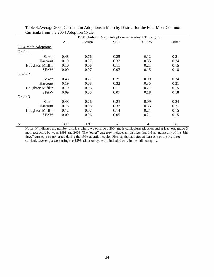
34
Table 4.Average 2004 Curriculum Adoptionsin Math by District for the Four Most Common
Curricula from the 2004 Adoption Cycle.
1998 Uniform Math Adoptions – Grades 1 Through 3
All Saxon SBG SFAW Other
2004 Math Adoptions Grade 1
Saxon 0.48 0.76 0.25 0.12 0.21 Harcourt 0.19 0.07 0.32 0.35 0.24
Houghton Mifflin 0.10 0.06 0.11 0.21 0.15 SFAW 0.09 0.07 0.07 0.15 0.18
Grade 2 Saxon 0.48 0.77 0.25 0.09 0.24
Harcourt 0.19 0.08 0.32 0.35 0.21 Houghton Mifflin 0.10 0.06 0.11 0.21 0.15
SFAW 0.09 0.05 0.07 0.18 0.18 Grade 3
Saxon 0.48 0.76 0.23 0.09 0.24 Harcourt 0.18 0.08 0.32 0.35 0.21
Houghton Mifflin 0.12 0.07 0.14 0.21 0.15 SFAW 0.09 0.06 0.05 0.21 0.15
N 286 128 57 34 33
Notes: N indicates the number districts where we observe a 2004 math-curriculum adoption and at least one grade-3
math test score between 1998 and 2008. The “other” category includes all districts that did not adopt any of the “big
three” curricula in any grade during the 1998 adoption cycle. Districts that adopted at least one of the big-three
curricula non-uniformly during the 1998 adoption cycle are included only in the “all” category.
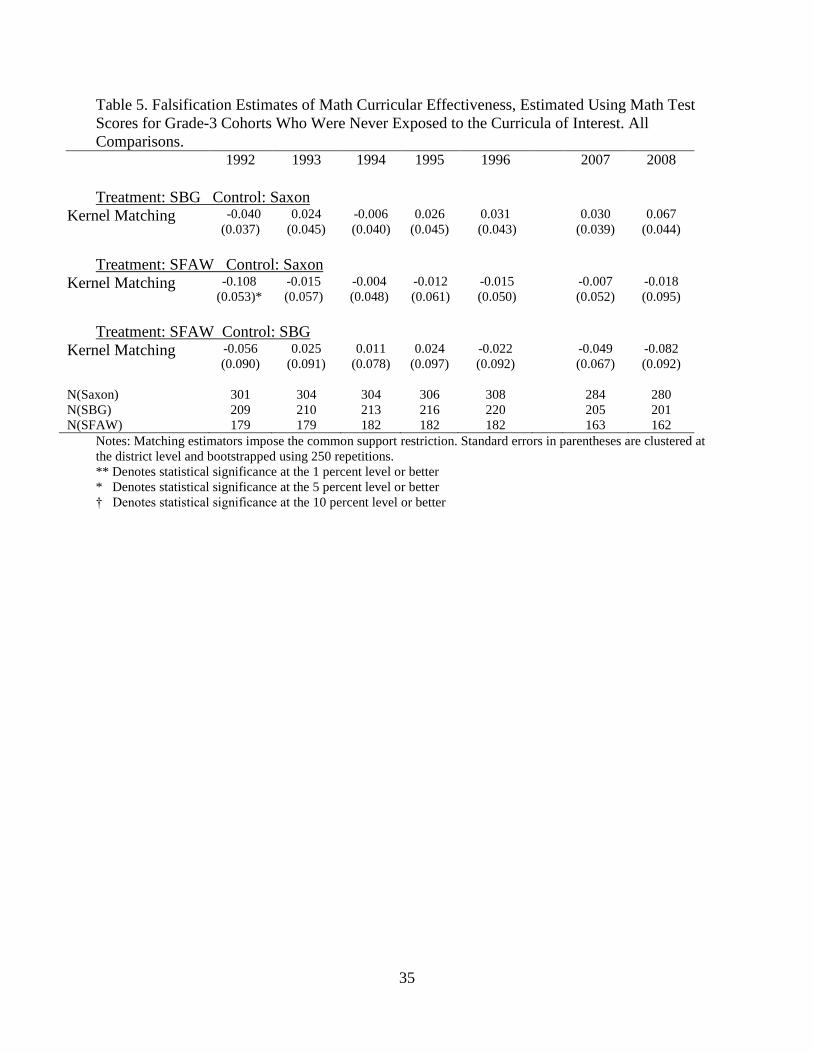
35
Table 5. Falsification Estimates of Math Curricular Effectiveness, Estimated Using Math Test
Scores for Grade-3 Cohorts Who Were Never Exposed to the Curricula of Interest. All
Comparisons.
1992 1993 1994 1995 1996 2007 2008
Treatment: SBG Control: Saxon
Kernel Matching -0.040
(0.037)
0.024
(0.045)
-0.006
(0.040)
0.026
(0.045)
0.031
(0.043)
0.030
(0.039)
0.067
(0.044)
Treatment: SFAW Control: Saxon
Kernel Matching -0.108
(0.053)*
-0.015
(0.057)
-0.004
(0.048)
-0.012
(0.061)
-0.015
(0.050) -0.007
(0.052)
-0.018
(0.095)
Treatment: SFAW Control: SBG
Kernel Matching -0.056
(0.090)
0.025
(0.091)
0.011
(0.078)
0.024
(0.097)
-0.022
(0.092) -0.049
(0.067)
-0.082
(0.092)
N(Saxon) 301 304 304 306 308 284 280
N(SBG) 209 210 213 216 220 205 201
N(SFAW) 179 179 182 182 182 163 162
Notes: Matching estimators impose the common support restriction. Standard errors in parentheses are clustered at
the district level and bootstrapped using 250 repetitions.
** Denotes statistical significance at the 1 percent level or better
* Denotes statistical significance at the 5 percent level or better
† Denotes statistical significance at the 10 percent level or better
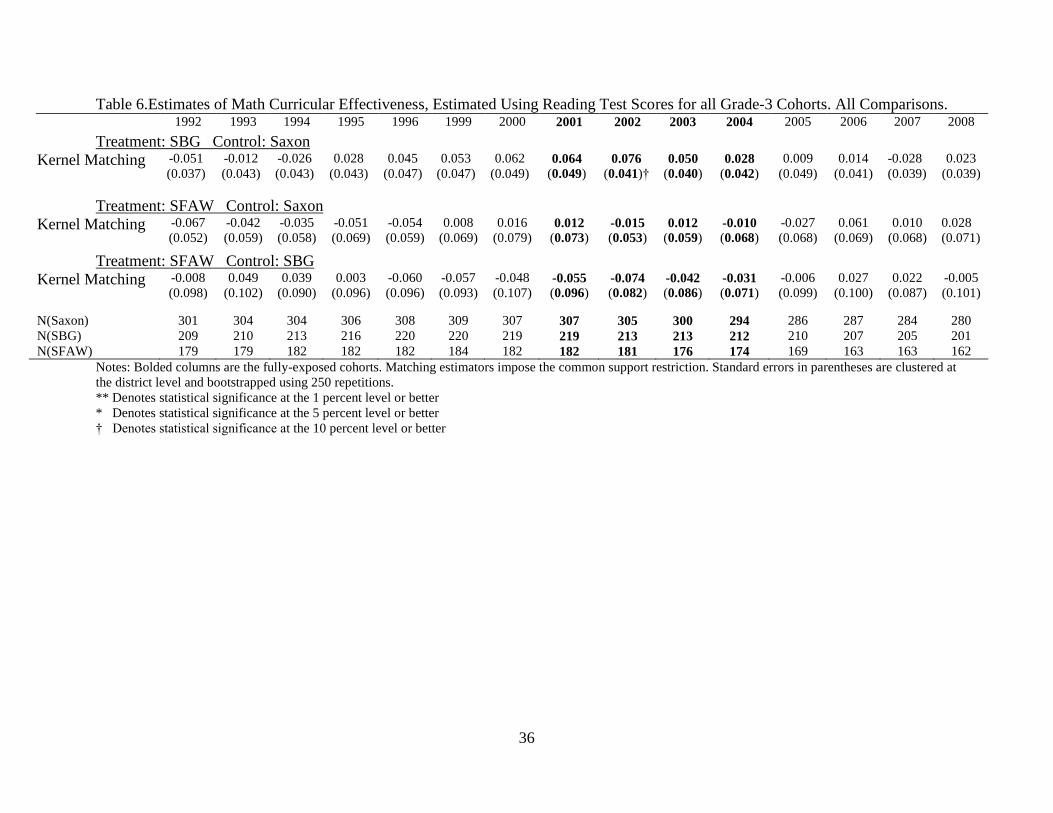
36
Table 6.Estimates of Math Curricular Effectiveness, Estimated Using Reading Test Scores for all Grade-3 Cohorts. All Comparisons.
1992 1993 1994 1995 1996 1999 2000 2001 2002 2003 2004 2005 2006 2007 2008
Treatment: SBG Control: Saxon
Kernel Matching -0.051
(0.037)
-0.012
(0.043)
-0.026
(0.043)
0.028
(0.043)
0.045
(0.047)
0.053
(0.047)
0.062
(0.049) 0.064
(0.049) 0.076
(0.041)†
0.050
(0.040)
0.028
(0.042)
0.009
(0.049)
0.014
(0.041)
-0.028
(0.039)
0.023
(0.039)
Treatment: SFAW Control: Saxon
Kernel Matching
-0.067
(0.052)
-0.042
(0.059)
-0.035
(0.058)
-0.051
(0.069)
-0.054
(0.059)
0.008
(0.069)
0.016
(0.079) 0.012
(0.073) -0.015
(0.053) 0.012
(0.059) -0.010
(0.068)
-0.027
(0.068)
0.061
(0.069)
0.010
(0.068)
0.028
(0.071)
Treatment: SFAW Control: SBG
Kernel Matching -0.008
(0.098)
0.049
(0.102)
0.039
(0.090)
0.003
(0.096)
-0.060
(0.096)
-0.057
(0.093)
-0.048
(0.107) -0.055
(0.096) -0.074
(0.082) -0.042
(0.086) -0.031
(0.071)
-0.006
(0.099)
0.027
(0.100)
0.022
(0.087)
-0.005
(0.101)
N(Saxon) 301 304 304 306 308 309 307 307 305 300 294 286 287 284 280
N(SBG) 209 210 213 216 220 220 219 219 213 213 212 210 207 205 201
N(SFAW) 179 179 182 182 182 184 182 182 181 176 174 169 163 163 162
Notes: Bolded columns are the fully-exposed cohorts. Matching estimators impose the common support restriction. Standard errors in parentheses are clustered at
the district level and bootstrapped using 250 repetitions.
** Denotes statistical significance at the 1 percent level or better
* Denotes statistical significance at the 5 percent level or better
† Denotes statistical significance at the 10 percent level or better