Proc. Nati. Acad. Sci. USAVol. 78, No. 4, pp. 1981-1985, April 1981Applied PhysicU and Mathematical Sciences

Large-scale flow generation in turbulent convection(instability/transition/turbulence/large-scale order)

RUBY KRISHNAMURTI* AND Louis N. HOWARDt*Department of Oceanography, Florida State University, Tallahassee, Florida 32306; and tDepartment of Mathematics, Massachusetts Institute of Technology,Cam ridge, Massachusetts 02139

Contributed by Louis N. Howard, January 5, 1981

ABSTRACT In a horizontal layer of fluid heated from belowand cooled from above, cellular convection with horizontal lengthscale comparable to the layer depth occurs for small enough valuesof the Rayleigh number. As the Rayleigh number is increased,cellular flow disappears and is replaced by a random array of tran-sient plumes. Upon further increase, these plumes drift in onedirection near the bottom and in the opposite direction near thetop of the layer with the axes of plumes tilted in such a way thathorizontal momentum is transported upward via the Reynoldsstress. With the onset of this large-scale flow, the largest scale ofmotion has increased from that comparable to the layer depth toa scale comparable to the layer width. The conditions for occur-rence and determination of the direction of this large-scale cir-culation are described.

This is a report on a laboratory study of convection in a hori-zontal layer of fluid uniformly and steadily heated from belowand cooled from above. This is the arrangement that leads tocellular convection for a range of values of the Rayleigh number(the dimensionless measure of temperature difference, definedbelow) sufficiently small but greater than a critical value. Thehorizontal scale of these cells is comparable to the depth d ofthe layer. At successively larger values ofthis parameter, a num-ber of transitions in the flow pattern as well as in the heat fluxare observed (1-6). Most ofthese changes are within the regimeof cellular flows.We shall describe here a further transition which leads to a

very different scale of motion and very different transport prop-erties. In this regime the flow is no longer cellular. It is a flowhaving primarily two scales of motion. The smaller scale flow,with horizontal scale comparable to the layer depth d, is bestdescribed as transient bubbles or plumes that have an organizedtilt away from the vertical. The larger scale flow, having scaleL, is a horizontal flow with vertical shear such that the flow isoppositely directed near the bottom and the top. L is usuallythe container width which, in these experiments, is an orderof magnitude larger than d. The large-scale flow is apparentlymaintained against viscous dissipation by the Reynolds stressdivergence of the tilted plume motions.

APPARATUS AND PROCEDUREThe convecting fluid occupied a space ofdepth d and horizontalextent L by L such that d/L was a small number (of order 102to 10-l). Most of the new results reported below were obtainedwith d = 2 and 5 cm, L = 48 cm. The fluid layer was boundedabove and below by metal blocks whose thermal conductivitywas several thousand times that ofthe liquids used. Even in themost extreme case within this set of experiments, when theconvective heat flux was 30 times the conductive heat flux, theboundaries had conductivity 2 orders of magnitude higher than

the effective conductivity of the fluid layer. Thus, the boundarycondition was one of constant temperature along both top andbottom boundaries. On all its lateral boundaries, the fluid layerwas bounded and insulated by 3 cm of Plexiglas and 5 cm ofStyrofoam. Normally the apparatus was leveled so that its slopewas no more than 0.0006 cm in 30 cm. The flatness and par-allelism of the horizontal boundaries were comparable to this.The fluids used were water and some of the silicone oils.

The auxiliary equipment for control and measurement ofheatflux are described briefly here and in detail in ref. 3. In additionto the convecting layer, six layers of solid materials, each 51 cmsquare, were used in a stack. The bottom layer was a 10-cm-thick aluminum block with the heater (made of a fine mesh ofresistance material) attached to its bottom. Above this lay a 0.64-cm-thick Plexiglas layer and above this a 5-cm-thick copperlayer. Above this lay the convecting fluid. Above the fluid were5 cm of copper, then 0.64 cm of Plexiglas, and then a 10-cmaluminum block containing channels for circulating coolingfluid. (In some of the earlier experiments, 2.5-cm-thick alu-minum blocks were used in place ofthe copper blocks.) The low-conductivity Plexiglas gives rise to measurably large tempera-ture differences between the metal blocks and was used to mea-sure the total heat flux [a method devised by Malkus (1)]. Theentire stack was placed in a Plexiglas tank which was surroundedon all sides by Styrofoam 5 cm thick.

The procedure was to set the heater voltage and then adjustthe temperature of the cooling water so that, when the tem-peratures measured in the four metal blocks reached steadystate, the mean temperature of the convecting fluid remainedat room temperature. Thus, the total heat flux H was prescribed(although not measured) by the input voltage. The temperaturewas constant on the top and bottom boundaries of the fluid, butthe magnitude ofthe difference ATbetween these constants wasdetermined indirectly through the convective heat flux of thefluid.

The Rayleigh number was computed from the measured AT.The total heat flux H through the fluid was equated to the con-ductive flux through either of the Plexiglas layers. The con-ductivity of the Plexiglas was determined in terms ofthe knownconductivity ofwater by performing the experiment with water0.5 cm deep and AT smaller than the critical value for onset ofconvection.

To study the geometry of the time-dependent flow, the fol-lowing arrangement was used to obtain (x, t) photographs fromwhich information about the Eulerian velocity could be de-duced. Here x refers to the horizontal coordinate along a fixedline within the fluid, perpendicular to the optic axis of the cam-era, and t refers to the time. We also let y be the coordinatealong the optic axis and z the vertical coordinate. The fluid con-tained suspended tracer particles (small light-reflecting flakes)that became aligned by the shear of the flow. The illuminatedregion was 2-3 mm in diameter, 48 cm long along x, and chosento lie near either the bottom or the top of the fluid layer. The

1981

The publication costs ofthis article were defrayed in part by page chargepayment. This article must therefore be hereby marked "advertise-ment" in accordance with 18 U. S. C. §1734 solely to indicate this fact.

Dow

nloa

ded

by g

uest

on

May

3, 2

020

1982 Applied Physical and Mathematical Sciences: Krishnamurti and Howard Proc. Natl. Acad. Sci. USA 78 (1981)

lightsused were either two 2-W zirconium arc lamps or a 5-mWcontinuous laser.

With the illuminated region fixed in space, a wedge wasmoved under the camera in such a way that the camera wouldrotate about a horizontal axis (parallel to the x axis) through itslens. The resulting photograph showed x along the abscissa andt along the ordinate. For example, if x were a line near the bot-tom of the layer, perpendicular to the longitudinal axis of rollconvection cells, the (x, t) photograph would be as shown in Fig.2a. A tracer particle within the illuminated region and properlyoriented so as to send light into the camera produced a markon the film. Individual particles generally remained in this re-gion long enough to make a short line segment in the picture,as is clearly seen in Fig. 2a. The local slope dx/dt ofthe directionfield in the (x, t) photograph produced by these line segmentsgave the horizontal velocity component as a function of x andt. Cell boundaries, from which fluid is diverging or towardwhich it is converging, are readily identified not only from thisdivergence or convergence but from changes in the generalbrightness or darkness brought about by the tendency of theflakes to become oriented in regions of high shear. In steadyconvection, as in Fig. 2a, cell boundaries remained fixed for alltime.

Stray heat sources that might produce lateral temperaturegradients were minimized by the physical arrangement of theequipment. The convection tank and the photographic appa-ratus were enclosed in a light-tight housing. Except for thelights, the motor drive for the camera, and the heater for thefluid layer, all other heat-producing instruments of control ormeasurement (apart from the experimentalist) were kept out-side this housing.

After the large-scale flow was detected, several additions tothe apparatus were made to test what controlled the directionof this circulation. The first was a paddle made of 0.32-cm-di-ameter stainless steel rod, 47 cm long, which could be drawnin the x direction perpendicular to its length. The second ad-dition was a jack to tilt the entire apparatus. The third was theaddition of a heater in the side boundary of the fluid layer. A35-cm length of nichrome wire was embedded in a 0.64-cm-thick sheet of Plexiglas. This sheet replaced a similar one thatwas part of the side wall. The heater wire occupied a horizontalposition approximately 1 cm higher than the bottom of the con-vecting layer and 1.3 cm outside the fluid.

Finally, the large-scale circulation was also observed in a cy-lindrical annular tank of fluid uniformly heated below andcooled above. The diameter of the outer Plexiglas cylinder was

45.8 cm, the gap width between the two cylinders was 4.3 cm,and the fluid depth d was 10.6 cm. The lid was floated on an

air bearing but restrained from rotating except for tests of theeffect of imposed motion of the lid upon direction of large-scalecirculation. For cooling the top boundary, the lid carried a vol-atile fluid open to the air.

OBSERVATIONSFig. 1 summarizes some observations of the flow found in thevarious ranges of the parameters. These parameters are theRayleigh number R and the Prandtl number P defined as

follows:

R = g ATd3, p =-KV K

where g is the acceleration ofgravity, a is the thermal expansioncoefficient, K iS the thermal diffusivity, v is the kinematic vis-cosity, d is the depth of the fluid layer, and AT is the temper-ature difference between bottom and top boundaries. The new

observations refer to flows found to the upper left of the curve

labeled V in Fig. 1. To the lower right of this curve the flows

are cellular: as labeled, the flow is steady two-dimensional inthe range between curves I and II. It is steady three-dimen-sional cellular between curves II and III, and time-dependent(quasi-periodic), three dimensional, and cellular betweencurves III and V. By cellular we mean that a fluid parcel initiallyat some horizontal location is always confined to the vicinity ofthat location, horizontal excursions being limited by cell bound-aries that have horizontal separation comparable to the layerdepth. (This is certainly so between curves I and III and at leastlargely so between curves III and V.) Because most of thesestates are history dependent, the actual transition point variesdepending upon how it was attained. Fig. 1 obtains when thestate of the system was reached from lower values of Rayleighnumber, by small increments in R. Further explanation can befound in ref 5.

Curve V was defined in ref 2 as the Rayleigh number abovewhich irregular fluctuations in temperature at a point mid-depthin the fluid layer were nearly always present. Although some-what subjective, it is a useful criterion.One of the major differences between the flows occurring to

the upper left of curve V and those to the lower right is seenin the (x, t) photographs in Fig. 2. Fig. 2 b and c show a linein the fluid layer 0.2 cm above the bottom boundary. Fig. 2b,at R = 106 and P = 0.86 X 103, is for parameter values to theright of curve V. Fig. 2c, at R = 106 but P = 7, is to the left ofcurve V. In Fig. 2b there are cell boundaries which, althoughthey may oscillate laterally, are always identifiable. In Fig. 2c,there are no cell boundaries. Fig. 2b is a cellular flow with brightor dark regions moving repeatedly from one cell boundary toa neighboring one. These regions have been shown (5) to cor-

respond to hot or cold spots convected around the cell. In Fig.2c, hot bubbles or plumes off the bottom, randomly spaced inposition and time, form and vanish. Cold bubbles off the toplikewise form and vanish, much as described by the bubblemodel (7). At any instant of time, their horizontal spacing isapproximately d or somewhat less. It should be pointed out alsothat Fig. 2c is not an initial transient state; it is the statisticallysteady state that is observed 1 hr or 100 hr after convection isstarted.At P = 7 and R = 5 X 104, the flow is similar to Fig. 2b, so

that increasing R at fixed P also leads to the change of flow de-picted from Fig. 2b to Fig. 2c.

The other major difference-and the one to which we par-ticularly wish to call attention in this report-is seen in Fig. 2dwhich shows an (x, t) photograph for P = 7 and R = 2.4 X 106,taken 0.2 cm above the bottom boundary. It shows that theplumes have a net drift from left to right with an average speedof 7 X 10-2 cm sec1. A similar photograph taken 0.2 cm belowthe top showed plumes drifting from right to left with the sameaverage speed.

From the (x, t) photographs it is not known if this apparentmotion is a wave propagation or if there is an associated mass

flux. Thymol blue was added to the water so that neutrally buoy-ant dye could be produced at an electrode, and the dyed fluidwas followed with time. Fig. 3 shows a sequence, at 30-sec in-tervals, of a vertical slice (x, z) view of the fluid. In this case thelayer depth was 10 cm. The dye front along the bottom pro-gressed at an average speed fi of 3 X 10-2 cm sec&1 from leftto right and actually reached the opposite wall, by which timeit was quite diffuse. These magnitudes are not easily comparedfrom case to case because only the x component, fi, is measured,whereas in some repetitions of the experiment there was a ve-

locity component v3 in the y direction as well. Maximum valuesof ft on the order of 10-1 cm sec' have been observed.

In Fig. 3, as the dyed fluid became buoyant, it rose into theinterior of the layer where it became entangled in the motionofthe plume. It often rose to become caught in the leftward drift

Dow

nloa

ded

by g

uest

on

May

3, 2

020

Applied Physical and Mathematical Sciences: Krishnamurti and Howard Proc. NatI. Acad. Sci. USA 78 (1981)

Turbulent fli

TimeIflow

lo-2 ,10I 10

Steady two-dimensional flow FIG. 1. Regime diagram. o, Steady cellularflow; e, time-dependent cellular flow; O, cellsand transient bubbles (transitional); A, tran-

102 103 104 sient bubbles; _, large-scale flow with tiltedplumes; *, heat flux transitions (see text and ref.

PRANDTL NO. 5 for further explanation).

at the top of the layer. A general tilt of the plumes from lowerright to upper left can be discerned even though the flow was

quite turbulent. Thus, we conclude that there is not only a (timeand/or horizontal) mean Eulerian velocity fi(z) but also a nethorizontal Lagrangian transport extending the entire width ofthe tank. Observations of the occurrence of cells, plumes, andlarge-scale flow in various regions of parameter space are sum-

marized in Fig. 1.On repetitions of the experiment, the large-scale flow was

seen to be sometimes from left to right along x at the bottomand from right to left along x at the top (ft counterclockwise).On other realizations, the flow was clockwise. On still others,the large-scale flow was in the y direction (v) and either clock-wise or counterclockwise. It may also be at some other angleto the x direction. When the flow was and clockwise, this flowwas often nearly independent of y but, on another repetition,it might be that the center of the large-scale rising was at theleft wall at some value of y; at other values of y, the center ofthe rising wandered to other values of x.

When this large-scale flow was first discovered, various testswere made to see if it were inadvertently being driven directlyby horizontal asymmetries. The leveling of the apparatus was

checked. Horizontal temperature gradients in the boundarieswere measured to check the possibility of malfunction of thecooling or heating system. In the aluminum blocks with theheater, or the cooler, horizontal gradients were oforder 10-30Cacross 35 cm. In the middle two (copper) blocks, which do notcontain any thermal forcing, the horizontal gradients were

larger: 10-20C in 25 cm. However, this magnitude of horizontalgradient would drive, in water, a horizontal velocity u =10-3cm sec6 I which is 2 orders ofmagnitude smaller than observed.Although horizontal asymmetries certainly must be present,due to errors in leveling the apparatus or to small differencesin temperature of the Plexiglas side walls, these had no ob-servable effect at lower Rayleigh number, or even at the same

Rayleigh number (with the same ratio of side wall area to hor-izontal area), when a higher Prandtl number fluid was used andno large-scale flow was observed.

Convinced that the large-scale flow was not externally driven,we attempted to check, as to order ofmagnitude, that the large-scale flow and the tilt of the plumes were consistent with theReynolds equations relating a (time- and horizontal-) mean flowwith the Reynolds stress associated with fluctuations. The prin-

cipal equation here is the mean horizontal momentum equationwhich, if the tank were horizontally unbounded (or in the caseof the cylindrical annulus), is:

[1]

The overbar indicates a horizontal and time average, u' and w'are the fluctuations from the mean, and v is the kinematic vis-cosity. (With the finite horizontal extent there could conceiv-ably also be a nonzero mean horizontal pressure gradient termin this equation-which indeed might well be important were

there external driving-but we omit this here.) Integrating ver

tically from the bottom wall we obtain u'w' = >i{si - w), usjbeing the mean shear at the wall. Now, for a rough estimate wemay perhaps suppose that the mean flow is has a profile in z

something like = - U sin(2i7rz/d), taking the origin of z at thecenter of the fluid layer so -d/2 < z < d/2. This would cor-

respond to a Reynolds stress uVw' = (4irUv/d) cos2(irz/d).Thus, with U - 0, corresponding to flow from left to right inthe lower half of the layer (as in Fig. 3), uVw' must be negativeand its maximal magnitude, achieved at the center, should beabout 10v/d times the maximum of ft. Detailed measurementsof the fluctuating velocity components u' and w', and of theircorrelation, have not yet been made. However visual obser-vation and photographs like Fig. 3, together with the (x, t) pho-tographs, indicate the following. (i) The fluctuations are on thewhole associated with motions in the tilting plumes. (ii) Theplumes tilt in such a way (about 450 from lower right to upperleft in cases such as shown in Fig. 3) that uV' has sign oppositeto that of ft in the lower halfand w' is characteristically of aboutthe same magnitude as U'. (iii) The maximal magnitudes of u',w', and all are about 0.1 cm sec1 in our experiments in whichthe large-scale flow is observed.We thus may estimate uVw' as about 0.2 X 10-2 cm2 sec-2

if we include factors of about 1/2 for the x average (assumingu' and w' have sinusoidal variation with x) and also for the timeaverage. The last is a rough estimate from the fraction ofthe time

that plumes are seen at any location on the (x, t) photographs.With d = 5 cm and Is = 0.01 cm2 sec' we get (10v/d)tm1nax0.2 X 10-2 cm2 see-2, so there does not appear to be any clearinconsistency with the Reynolds equation (Eq. 1). One may

regard the mean flow as being "driven" by the Reynolds stressassociated with the tilting plumes. We emphasize that such a

lO0

o lo5z

x

-J

< 104

I0

1983

I I=(Uw PU-,.

Dow

nloa

ded

by g

uest

on

May

3, 2

020

1984 Applied Physical and Mathematical Sciences: Krishnamurti and Howard Proc. Nati. Acad. Sci. USA 78 (1981)

b

c

d

FIG. 2. (x, t) representations of the flow 0.2 cm above the bottomboundary. The range in x along the abscissa is 0 to 45 cm; t increasesdownward; range in time is 0 to T. (a) R = 7.5 x 104, P = 0.86 x 103,T = 17 min. (b) R = 106 P = 0.86 x 103, T = 22 min. (c) R = 106, P= 7, T = 22 min. (d) R = 2.4 x 106, P = 7, T = 9 min.

statement is a description, not an explanation, of the large-scaleflow. The Reynolds equation would also be consistent with no

mean flow, and no tilting ofthe plumes-and in fact this appearsto be what occurs below a Rayleigh number of about 2 x 106in water. The theoretical understanding of why this transitionoccurs and why it occurs at R = 2 X 106 remains a challenge.

The phenomenon seems to resemble the onset of steady con-

vection in that the physically realized "state" changes to one ofa set, each member of which individually has less symmetrythan the equations and boundary conditions describing themotion. Such symmetry-breaking occurs in many mathematicalmodels involving changes of stability of stationary or periodicsolutions and associated bifurcations, and Rayleigh's explana-tion of the onset of cellular convection in such terms has beenfollowed in spirit by essentially all of the many subsequent ex-

plorations ofother aspects ofcellular convection. Whether suchconcepts as stability and bifurcation can contribute usefully toan understanding of a transition entirely in the turbulent rangeseems less clear; this report, in any case, is about the obser-vation of the transition, not its theoretical interpretation.What determines the direction of the large-scale flow? We

were not successful in altering the direction of the established

FIG. 3. Sequence of views of (x, z) slice through convecting fluid,showing the rightward progress of dye along bottom and the lowerright to upper left tilt of plumes.

large-scale flow by drawing the paddle along the bottom of theconvecting layer, although we tried various speeds includingone approximately the speed ofthe large-scale flow. We did notattempt this while the Rayleigh number was being increasedthrough R1 2 X 106. It was not possible to match the timescales involved. Similarly, in the annular tank it was not possibleto alter the direction of the already established large-scale flowby rotating the lid through one revolution, at various speeds,in either the clockwise or counterclockwise direction.When the entire convection tank was tilted at various angles

up to a maximum of 0.23 degrees, neither the already estab-lished large-scale flow nor the large-scale flow that set in as Rwas increased from zero to >2 X 106 was determined by thetilt ofthe layer. Certainly it is known that, ifthe tilt angle is largeenough, the direction of the flow is determined by that tilt butfor the tilts used here (which were 102 times larger than any tiltofthe layer due to leveling error) there was no such determination.When the fluid layer was heated from the side, the direction

of the large-scale flow could be determined when the heatingrate was large enough. Several different heating rates weretried. For example, when the power to the side heater was 3W, this heating rate did not reverse an already established large-

Dow

nloa

ded

by g

uest

on

May

3, 2

020

Applied Physical and Mathematical Sciences: Krishnamurti and Howard Proc. NatI. Acad. Sci. USA 78 (1981) 1985

scale flow. The rising motion induced at the heated side wallwas accompanied by sinking motion a short distance (<d) away,and the rest of the layer behaved as without the side heating.When the side heater, at 3 W, was on while R was increasedfrom zero through 2 x 106, the direction of the large-scale flowwas not determined by the side on which the heater was placed.However, when the heating was at 11 W, as R was increasedfrom zero to 2 x 106 the large-scale flow was ti, clockwise, whenthe heater was on the left, and fi, counterclockwise, when theheater was on the right.

Furthermore, at 11 W, an established large-scale flow couldbe made to reverse direction by switching the heater to theother side of the tank. The response was within an hour; thethermal diffusion time ofthe Plexiglas spacer was approximatelyone-half hour. Also, after the side heater was turned off, thedirection ofthe large-scale flow remained-unchanged for severaldays thereafter. This was with R = 107. The heating at 11 Wcaused an increase in temperature of approximately 1MC at theoutside of the Plexiglas spacer, about 1 cm from the fluid. Thetemperature difference in the vertical was 20C. This heatingalone, with the vertical Rayleigh number R = 0, produced a

large-scale overturning with horizontal velocity u(x) measuredat a distancez = 0.2 cm below the top of the 5-cm-deep layer.The measurement was conveniently made from the slopes ofparticles in an (x, t) photograph. The maximum u, which oc-

curred at x = 14 cm from the heated wall, for z = 0.2 cm, was8 x 10-' cm sec-1. This is still 1 order of magnitude less thanthe ui produced by the tilting plumes.

Finally, large-scale flow was observed in the cylindrical an-

nulus, showing that a pressure difference between two lateral

4.20

3.60-

*.

3.00-

O 2.40.

x /'

t~~~~~~~~0 ,,/X

1.80 ,

1.20 r , -I

0.60 ;,'.

0.0010.00 0.70 1.40 2.10 2.80

R, x 10-6

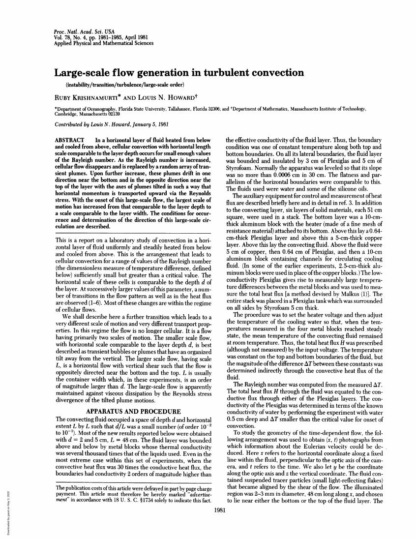
FIG. 4. Heat flux H vs. Rayleigh number R. H has been nondi-mensionalized to equal N x R (N is the Nusselt number). The coor-

dinate scale is appropriate for the data shown by dots. For +, the scaleshould be decreased by a factor 10. A least-squares fit of segments ofdata to a straight lineNR = aR + b gave a = 5.05 for the line labeledI, a = 8.40 for II, and a = 10.7 for III. The change in slope at R = 1.1x 106 may be associated with the onset of the large-scale circulationwhich is seen atR 2 x 106.

boundaries is not necessary to produce this flow. The small-scaleplumes were considerably narrower than the depth d of thelayer, but they tilted approximately 450 and in this sense theyoccupied a horizontal distance of about d. The large-scale flowwas observed to continue around the annulus, in one directionnear the bottom and in the opposite direction near the top. Withthe geometry thus unbounded in x, the large-scale flow hashorizontal wave number 0.

Movies of the flow in the annulus and of an (x, z) slice in thesquare tank are available.The heat flux, nondimensionalized to equal the Nusselt num-

ber times the Rayleigh number, is plotted against Rayleighnumber in Fig. 4. (The Nusselt number is the ratio of total heatflux to conductive heat flux.) Discrete changes in slope wereseen at Rayleigh numbers RI,, = 3.3 X 104, RIv = 5.5 X 104,Rv = 1.0 X 105, RvI = 5.0 X 105, and RvII = 1.1 X 106, thelast three ofwhich are shown in Fig. 4. Some ofthese are in goodagreement with the Malkus heat flux transitions RIM = 3 X 104,RIv = 5.5 X 104, Rv = 1.7 X 10, RvI = 4.1 X 10, RvjI = 8.5x 105, and RvIII = 1.6 X 106. It appears that the onset of thelarge-scale circulation might be associated with the slope changeat RvII = 1.1 X 106.

DISCUSSIONAs the Rayleigh number is increased, cellular flow vanishes andis replaced by a flow that has no permanent cell boundaries. Itconsists of hot rising and cold sinking transient bubbles orplumes. At still higher R, the plumes drift in one direction nearthe bottom, in the opposite direction near the top of the layer,and tilt from the vertical and thereby transport mean horizontalmomentum in the vertical direction. When viewed in the (x,t) representation, the transition is reminiscent of a phase tran-sition. When there are cell boundaries as in Fig. 2a, fluid parcelsare forever confined to circulate in the lattice-like confines ofthe cell walls. In Fig. 2b, plumes appear but are constrainedby the cell walls to circulate within the cell. In Fig. 2c the cellboundaries have vanished and, as R is increased further in Fig.2d, the "melt" begins to flow. The largest scale of motion whichwas previously equal to the depth d has suddenly changed tothe layer width L. The appearance of this new large scale hasmany implications. Turbulent horizontal transport of a passivetracer is completely changed when this large-scale flow sets in.Continental drift and sea floor spreading, which have generallybeen thought to require deep convection in the mantle to ex-plain the large scales observed at the crust, might perhaps beviewed in terms of a large-scale convective flow in the muchshallower but more plastic asthenosphere.

This work was supported by the Fluid Dynamics Division of theOffice ofNaval Research and by the National Science Foundation (GrantOCE-772-7939). This is Geophysical Fluid Dynamics Institute contri-bution 162.

1. Malkus, W. V. R. (1954) Proc. R. Soc. London Ser. A 225,185-195.

2. Willis, G. E. & Deardorff, J. W. (1967) Phys. Fluids 10, 931-937.3. Willis, G. E. & Deardorff, J. W. (1967) Phys. Fluids 10,

1861-1866.4. Krishnamurti, R. (1970) J. Fluid Mech. 42, 295-307.5. Krishnamurti, R. (1970) J. Fluid Mech. 42, 309-320.6. Busse, F. H. & Whitehead, J. A. (1971) J. Fluid Mech. 47,

305-320.7. Howard, L. N. (1966) Proceedings of the Eleventh International

Congress of Applied Mechanics, Munich, Federal Republic ofGermany, August 1964, ed. Gortler, H. (Springer, Berlin), pp.1109-1115.

Dow

nloa

ded

by g

uest

on

May

3, 2

020