Large-Scale L1-Related Minimization in Compressive Sensing ...plato.asu.edu/slides/zhang_cs.pdf · Large-Scale L1-Related Minimization in Compressive Sensing and ... Yilun Wang, Junfeng

CS Fundamental Missing Data Recovery Theory Challenges Algorithms FPC Total Variation

Large-Scale L1-Related Minimization inCompressive Sensing and Beyond

Yin Zhang

Department of Computational and Applied MathematicsRice University, Houston, Texas, U.S.A.

Arizona State University

March 5th, 2008


Outline

Outline:

CS: Application and TheoryComputational Challenges and Existing AlgorithmsFixed-Point Continuation: theory to algorithmExploit Structures in TV-Regularization

Acknowledgments: (NSF DMS-0442065)

Collaborators: Elaine Hale, Wotao YinStudents: Yilun Wang, Junfeng Yang


Compressive Sensing Fundamental

Recover sparse signal from incomplete data

Unknown signal x∗ ∈ Rn

Measurements: Ax∗ ∈ Rm, m < nx∗ is sparse (#nonzeros ‖x∗‖0 < m)

Unique x∗ = arg min{‖x‖1 : Ax = Ax∗} ⇒ x∗ is recoverable

Ax = Ax∗ under-determined, min‖x‖1 favors sparse xTheory: ‖x∗‖0 < O(m/ log(n/m)) ⇒ recoveryfor random A (Donoho et al, Candes-Tao et al ..., 2005)


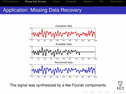
Application: Missing Data Recovery

0 100 200 300 400 500 600 700 800 900 1000−0.5

0

0.5Complete data

0 100 200 300 400 500 600 700 800 900 1000−0.5

0

0.5Available data

0 100 200 300 400 500 600 700 800 900 1000−0.5

0

0.5Recovered data

The signal was synthesized by a few Fourier components.


Application: Missing Data Recovery II

Complete data

Available data

Recovered data

75% of pixels were blacked out (becoming unknown).


Application: Missing Data Recovery III

Complete data

Available data

Recovered data

85% of pixels were blacked out (becoming unknown).


How are missing data recovered?

Data vector f has a missing part u:

f :=

[bu

], b ∈ <m, u ∈ <n−m.

Under a basis Φ, f has a representation x∗, f = Φx∗, or[AB

]x∗ =

[bu

].

Under favorable conditions (x∗ is sparse and A is “good”),

x∗ = arg min{‖x‖1 : Ax = b},

then we recover missing data u = Bx∗.


Sufficient Condition for Recovery

Feasibility: F = {x : Ax = Ax∗} ≡ {x∗ + v : v ∈ Null(A)}

Define: S∗ = {i : x∗i 6= 0}, Z ∗ = {1, · · · , n} \ S∗

‖x‖1 = ‖x∗‖1 + (‖vZ∗‖1 − ‖vS∗‖1) +(‖x∗S∗ + vS∗‖1 − ‖x∗S∗‖1 + ‖vS∗‖1

)> ‖x∗‖1, if ‖vZ∗‖1 > ‖vS∗‖1

x∗ is the unique min. if ‖v‖1 > 2‖vS∗‖1, ∀v ∈ Null(A) \ {0}.

Since ‖x∗‖1/20 ‖v‖2 ≥ ‖vS∗‖1, it suffices that

‖v‖1 > 2‖x∗‖1/20 ‖v‖2, ∀v ∈ Null(A) \ {0}


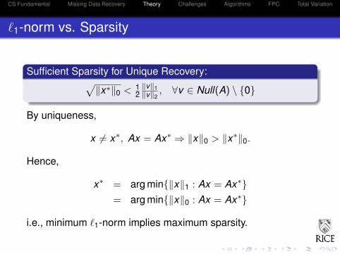
`1-norm vs. Sparsity

Sufficient Sparsity for Unique Recovery:√‖x∗‖0 < 1

2‖v‖1‖v‖2

, ∀v ∈ Null(A) \ {0}

By uniqueness,

x 6= x∗, Ax = Ax∗ ⇒ ‖x‖0 > ‖x∗‖0.

Hence,

x∗ = arg min{‖x‖1 : Ax = Ax∗}= arg min{‖x‖0 : Ax = Ax∗}

i.e., minimum `1-norm implies maximum sparsity.


In most subspaces, ‖v‖1 � ‖v‖2

In Rn, 1 ≤ ‖v‖1‖v‖2

≤√

n. However, ‖v‖1 � ‖v‖2 in mostsubspaces (due to concentration of measure).

Theorem: (Kashin 77, Garnaev-Gluskin 84)

Let A ∈ Rm×n be standard iid Gaussian. With probability above1− e−c1(n−m),

‖v‖1

‖v‖2≥ c2

√m√

log(n/m), ∀v ∈ Null(A) \ {0}

where c1 and c2 are absolute constants.

Immediately, for random A and with high probability

‖x∗‖0 <Cm

log(n/m)⇒ x∗ is recoverable.


Signs help

Theorem:There exist good measurement matrices A ∈ Rm×n so that if

x∗ ≥ 0 and ‖x∗‖0 ≤ bm/2c,

thenx∗ = arg min{‖x‖1 : Ax = Ax∗, x ≥ 0}.

In particular, (generalized) Vandermonde matrices (includingpartial DFT matrices) are good.

(“x∗ ≥ 0” can be replaced by “sign(x∗) is known”.)


Discussion

Further Results:Better estimates on constants (still uncertain)Some non-random matrices are good too(e.g. partial transforms)

Implications of CS:Theoretically, sample size n → O(k log (n/k))

Work-load shift: encoder → decoderNew paradigm in data acquisition?In practice, compression ratio not dramatic, but— longer battery life for space devises?— shorter scan time for MRI? ...


Related `1-minimization Problems

min{‖x‖1 : Ax = b} (noiseless)

min{‖x‖1 : ‖Ax − b‖ ≤ ε} (noisy)

min µ‖x‖1 + ‖Ax − b‖2 (unconstrained)

min µ‖Φx‖1 + ‖Ax − b‖2 (Φ−1 may not exist)

min µ‖G(x)‖1 + ‖Ax − b‖2 (G(·) may be nonlinear)

min µ‖G(x)‖1 + ν‖Φx‖1 + ‖Ax − b‖2 (mixed form)

Φ may represent wavelet or curvelet transform‖G(x)‖1 can represent isotropic TV (total variation)Objectives are not necessarily strictly convexObjectives are non-differentiable


Algorithmic Challenges

Large-scale, non-smooth optimization problems with densedata that require low storage and fast algorithms.

1k × 1k, 2D-images give over 106 variables.“Good" matrices are dense (random, transforms...).Often (near) real-time processing is required.Matrix factorizations are out of question.Algorithms must be built on Av and AT v .


Algorithm Classes (I)

Greedy Algorithms:Marching Pursuits (Mallat-Zhang, 1993)OMP (Gilbert-Tropp, 2005)StOMP (Donoho et al, 2006)Chaining Pursuit (Gilbert et al, 2006)Cormode-Muthukrishnan (2006)HHS Pursuit (Gilbert et al, 2006)

Some require special encoding matrices.


Algorithm Classes (II)

Introducing extra variables, one can convert compressivesensing problems into smooth linear or 2nd-order coneprograms; e.g. min{‖x‖1 : Ax = b} ⇒ LP

min{eT x+ − eT x− : Ax+ − Ax− = b, x+, x− ≥ 0}

Smooth Optimization Methods:Projected Gradient: GPSR (Figueiredo-Nowak-Wright, 07)Interior-point algorithm: `1-LS (Boyd et al 2007)(pre-conditioned CG for linear systems)`1-Magic (Romberg 2006)


Fixed-Point Shrinkage

min µ‖x‖1 + f (x) ⇐⇒ x = Shrink(x − τ∇f (x), τµ)

where Shrink(y , t) = sign(y) ◦max(|y | − t , 0)

Fixed-point iterations:

xk+1 = Shrink(xk − τ∇f (xk ), τµ)

directly follows from forward-backward operator splitting(a long history in PDE and optimization since 1950’s)Rediscovered in signal processing by many since 2000’s.Convergence properties analyzed extensively


Forward-Backward Operator Splitting

Derivation:

min µ‖x‖1 + f (x)

⇔ 0 ∈ µ∂‖x‖1 +∇f (x)

⇔ −τ∇f (x) ∈ τµ∂‖x‖1

⇔ x − τ∇f (x) ∈ x + τµ∂‖x‖1

⇔ (I + τµ∂‖ · ‖1)x 3 x − τ∇f (x)

⇔ {x} 3 (I + τµ∂‖ · ‖1)−1(x − τ∇f (x))

⇔ x = shrink(x − τ∇f (x), τµ)

min µ‖x‖1 + f (x) ⇐⇒ x = Shrink(x − τ∇f (x), τµ)


New Convergence Results

The following are obtained by E. Hale, W, Yin and YZ, 2007.Finite Convergence: for k = O(1/τµ)

xkj = 0, if x∗j = 0

sign(xkj ) = sign(x∗j ), if x∗J 6= 0

Rate of convergence depending on “reduced” Hessian:

lim supk→∞

‖xk+1 − x∗‖‖xk − x∗‖

≤κ(H∗EE)− 1κ(H∗EE) + 1

where H∗EE is the sub-Hessian corresponding to x∗ 6= 0.The bigger µ is, the sparser x∗ is, the faster is the convergence.


Fixed-Point Continuation

For each µ > 0,

x = Shrink(x − τ∇f (x), τµ) =⇒ x(µ)

Idea: approximately follow the path x(µ)

FPC:Set µ to a larger value. Set initial x .DO until µ it reaches its “right” value

Adjust stopping criterionStart from x , do fixed-point iterations until “stop”Decrease µ value

END DO


Continuation Makes It Kick

0 50 100 150

10−3

10−2

10−1

100

Iteration

||x −

xs||/

||xs||

(a) µ = 200

With ContinuationWithout Continuation

0 200 400 600 800

10−3

10−2

10−1

100

Iteration

(b) µ = 1200


Discussion

Continuation make fixed-point shrinkage practical.FPC appears more robust than StOMP and GPSR,and is faster most times. `1-LS is generally slower.1st-order methods slows down on less sparse problems.2-order methods have their own set of problems.A comprehensive evaluation is still needed.


Total Variation Regularization

Discrete (isotropic) TV for a 2D variable:

TV (u) =∑i,j

‖(Du)ij‖

(1-norm of 2-norms of 1st-order finite difference vectors)

convex, non-linear, non-differentiablesuitable for sparse Du, not sparse u

A mixed-norm formulation:

minu

µTV (u) + λ‖Φu‖1 + ‖Au − b‖2


Alternating Minimization

Consider linear operator A being a convolution:

minu

µ∑i,j

‖(Du)ij‖+ ‖Au − b‖2

Introducing wij ∈ R2 and a penalty term:

minu,w

µ∑i,j

‖wij‖+ ρ‖w − Du‖2 + ‖Au − b‖2

Exploit structure by alternating minimization:For fixed u, w has a closed-form solution.For fixed w , quadratic can be minimized by 3 FFTs.

(similarly for A being a partial discrete Fourier matrix)


MRI Reconstruction from 15% Fourier Coefficients

Original 250 x 250

SNR:14.74, t=0.09

Original 250 x 250

SNR:16.12, t=0.09

Original 250 x 250

SNR:17.72, t=0.08

Original 250 x 250

SNR:16.40, t=0.10

Original 250 x 250

SNR:13.86, t=0.08

Original 250 x 250

SNR:17.27, t=0.10

Reconstruction time ≤ 0.1s on a Dell PC (3GHz Pentium).


Image Deblurring: Comparison to Matlab Toolbox

Original image: 512x512 Blurry & Noisy SNR: 5.1dB. deconvlucy: SNR=6.5dB, t=8.9

deconvreg: SNR=10.8dB, t=4.4 deconvwnr: SNR=10.8dB, t=1.4 MxNopt: SNR=16.3dB, t=1.6

512× 512 image, CPU time 1.6 seconds


The End

Thank You!

Documents

Large-Scale L1-Related Minimization in Compressive Sensing ...plato.asu.edu/slides/zhang_cs.pdf · Large-Scale L1-Related Minimization in Compressive Sensing and ... Yilun Wang, Junfeng