Embed Size (px)
Citation preview
Financial support from the
Deutsche Forschungsgemeinschaft (German Research Foundation)
through grant GSC 111 is gratefully acknowledged.
Aachen Institute
for Advanced Study in
Computational Engineering Science
Large-scale linear regression:
Development of
high-performance routines
Alvaro Frank, Diego Fabregat-Traver and Paolo Bientinesi
arX
iv:1
504.
0789
0v1
[cs
.CE
] 2
9 A
pr 2
015

Large-scale linear regression: Development of
high-performance routines
Alvaro Frank, Diego Fabregat-Traver, and Paolo Bientinesi
AICES, RWTH Aachen, 52062 Aachen, Germany
Abstract. In statistics, series of ordinary least squares problems (OLS) are used to study
the linear correlation among sets of variables of interest; in many studies, the number of such
variables is at least in the millions, and the corresponding datasets occupy terabytes of disk
space. As the availability of large-scale datasets increases regularly, so does the challenge in
dealing with them. Indeed, traditional solvers—which rely on the use of “black-box” routines
optimized for one single OLS—are highly inefficient and fail to provide a viable solution for big-
data analyses. As a case study, in this paper we consider a linear regression consisting of two-
dimensional grids of related OLS problems that arise in the context of genome-wide association
analyses, and give a careful walkthrough for the development of ols-grid, a high-performance
routine for shared-memory architectures; analogous steps are relevant for tailoring OLS solvers
to other applications. In particular, we first illustrate the design of efficient algorithms that
exploit the structure of the OLS problems and eliminate redundant computations; then, we
show how to effectively deal with datasets that do not fit in main memory; finally, we discuss
how to cast the computation in terms of efficient kernels and how to achieve scalability.
Importantly, each design decision along the way is justified by simple performance models.
ols-grid enables the solution of 1011 correlated OLS problems operating on terabytes of data
in a matter of hours.
Keywords: Linear regression, ordinary least squares, grids of problems, genome wide associ-
ation analysis, algorithm design, out-of-core, parallelism, scalability
1 Introduction
Linear regression is an extremely common statistical tool for modeling the relationship between two
sets of data. Specifically, given a set of “independent variables” x1, x2, . . . , xp, and a “dependent
variable” y, one seeks the correlation terms βi, i = 1, . . . , p in the linear model
y = β1x1 + . . . βpxp. (1)
In matrix form, Eq. (1) is expressed as y = Xβ + ε, where y ∈ Rn is a vector of n “observations”,
the columns of X ∈ Rn×p are “predictors” or “covariates”, the vector β = [β1, . . . , βp]T contains the
“regression coefficients”, and ε is an error term that one wishes to minimize. In many disciplines,
linear regression is used to quantify the relationship between one or more y’s from the set Y, and
each of many x’s from the set X . The computational challenges raise from the all-to-all nature of
the problem (estimate how strongly each of the covariates is related to each of the observations),
and from the sheer size of the datasets Y and X , which often cannot be stored directly in main
memory.
One of the standard approaches to fit the model (1) to given y and X is by solving an ordinary
least squares (OLS) problem; in linear algebra terms, this corresponds to computing the vector β
such that
β =(XTX
)−1XTy.
In typical datasets, m, the number of available covariates (m = |X |), is much larger than p, the
number of variables actually used in the model. In this case, a group of l < p covariates is kept
fixed, and the remaining p − l slots are filled from X , in a rotating fashion; it is not uncommon
that the value p − l is very small, often just one, thus originating m ≥ m distinct OLS problems.
Mathematically, this means computing a series of βi’s such that
βi =(XT
i Xi
)−1XT
i y, where i = 1, . . . ,m; (2)
here Xi consists of two parts: XL, which contains l columns and is fixed across all m OLS problems,
and XRi , which instead contains p − l columns taken from X . In many applications, m can be of
the order of millions or even more.
When t > 1 dependent variables (t = |Y|) are to be studied against X , the problem (2) assumes
the more general form
βij =(XT
i Xi
)−1XT
i yj , (3)
where i = 1, . . . ,m, and j = 1, . . . , t, indicating that one has to compute a two-dimensional grid of
βij ’s, each one corresponding to an OLS problem. This is for instance the case in genomics (multi-
trait genome-wide association analyses) [1] and econometrics (explanatory variable exploration) [2].
Despite the fact that OLS solvers are provided by many libraries and languages (e.g., LAPACK,
NAG, MKL, Matlab, R), no matter how optimized those are, any approach that aims at computing
the 2D grid (3) via t × m invocations of a “black-box” routine is entirely unfeasible. The main
limitations come from the fact that this approach leads to the execution of inefficient and redundant
operations, lacks a mechanism to effectively manage data transfers from and to hard disk, and
underutilizes the resources on parallel architectures.
In this paper, we consider an instance of Eq. (3) as it arises in genomics, and develop ols-grid,
a parallel solver tailored for this application. Specifically, we focus on the study of omics data1 in the
context of genome wide association analyses (GWAA).2 Omics GWAA study the relation between
m groups of genetic markers and t phenotypic traits in populations of n individuals. In terms of
OLS, each trait is represented by a vector yj containing the trait measurements (one per individual);
each matrix Xi = [XL|XRi ] is composed of a set of l fixed covariates such as sex, age, and height
(XL), and one of the groups of r = p − l markers (XRi). A positive correlation between markers
XRiand trait yj indicates that the markers may have an impact in the expression of the trait.
Typical problem sizes in omics GWAA are roughly 103 ≤ n ≤ 105, 2 ≤ p ≤ 20 (with r = 1
or 2), 106 ≤ m ≤ 108, and 102 ≤ t ≤ 105. An exemplary analysis with size n = 30,000, p = 10
(l = 8, r = 2), m = 107, and t = 104, poses three considerable challenges. First, it requires the
computation of 1011 OLS problems, which, if tackled by a traditional “black-box” solver, would
perform O(1018) floating point operations (flops). Despite the fact that the problem lends itself to
a lower computational cost and efficient solutions, a black-box solver ignores the structure of the
problem and requires large clusters to obtain a solution. The second challenge is posed by the size of
the datasets to be processed: assuming single-precision data (4 bytes per element), a GWAA solver
reads as input about 2.4 TBs of data and produces as output 4 TBs of data. If the data movement
is not analyzed properly, the time spent in I/O transfers might render the computation unfeasible.
1 With the term omics we refer to large-scale analyses involving at least hundreds of traits [3,4,5].2 GWAA are often also referred to as genome wide association studies (GWAS) and whole genome associ-
ation studies (WGAS).
2
Finally, the computation needs to be parallelized and organized so that the potential of the current
multi-core and many-core architectures is fully exploited.
Contributions. This paper is concerned with the design and the implementation of ols-grid, a
high-performance algorithm for large-scale linear regression. While we use omics GWAA as a case
study, the discussion is relevant to a range of OLS-based applications. Specifically, we 1) illustrate
how to take advantage of the specific structure in the grid of OLS problems to design specialized
algorithms, 2) analyze the data transfers from and to disk to effectively deal with large datasets
that do not fit in main memory, and 3) discuss how to cast the computation in terms of efficient
kernels and how to attain scalability on many-core architectures. Moreover, by making use of simple
performance models, we identify the performance bottlenecks with respect to the problem size.
ols-grid, available as part of the GenABEL suite [6], allows one to execute an analysis of the
aforementioned size in less than 7 hours on a 40-core node.
Related work. Genome-wide association analyses received a lot of attention in the last decade [7].
Numerous high-impact findings have been reported, including but not limited to the identification
of genetic variations associated to a common form of blindness, type 2 diabetes, and Parkinson’s
disease [8,9,10,11]. A popular approach to GWAA is the so called Variance Components model,
which boils down to a set of equations similar to Eq. (3). The main difference with the present work
lies on the core equation, where one has to solve grids of generalized least squares (GLS) problems
instead of grids of OLSs. A number of libraries have been developed to carry out GLS-based GWAA,
the most relevant being FaST-LMM, GEMMA, GWFGLS, and OmicABEL [6,12,13,5].
OmicABEL, developed within our research group, showed remarkable performance improvements
with respect to the other existing methods [14,15]. Clearly, the same library can be used, by set-
ting the covariance matrix to the identity, to solve Eq. (3). While possible, this is not advisable:
OmicABEL reduces the two-dimensional grid of GLS problems to the grid of OLS problems
bij = (XTijXij)
−1XTij yj ,
which is deceivingly similar to Eq. (3); however, the subtle differences in the dependencies (subindices)
of the design matrix X lead to a more expensive and less efficient algorithm. In Sec. 5 we show how
the new ols-grid outperforms OmicABEL-Eig considerably.
A number of tools are focused on OLS-based linear regression analyses for GWAA; among them,
we mention ProbABEL (also part of the GenABEL suite), GWASP, and BOSS [16,17,18]. GWASP
stands out for its elegant algorithmic approach and a performance-oriented design; a more detailed
discussion is given in Sec. 5.4.
Organization of the paper. The remainder of the paper is organized as follows. In Sec. 2 we describe
the design of an efficient algorithm that exploits problem-specific knowledge. In Sec. 3 we analyze
the data transfers and discuss possible limitations inherent to the problem at hand, while in Sec. 4
we focus on the high performance and scalability of our software. Section 5 presents performance
results. Finally, Sec. 6 draws conclusions and discusses future work.
2 From the problem specification to an efficient algorithm
In this section we discuss the steps leading to the core algorithm behind ols-grid. Starting from
an elementary and generic algorithm, we incrementally refine it into an efficient algorithm tailored
specifically for grids of OLS arising in GWAA studies. The focus is on the reduction of the compu-
tational complexity.
3
As a starting point to solve Eq. (3), we consider a most naive black-box solver consisting of two
nested loops (for each i and j) around a QR-based algorithm for OLS [19]:
{Q,R} := qr(X)
b := R−1QT y.
Since the design matrix X only depends on the index i, the loop ordering i, j makes it possible to
compute the QR factorization once and reuse it across the j loop. Even with this simple code motion
optimization, this first algorithm performs substantial redundant calculations due to the structure
of Xi.
Recall that each matrix Xi can be logically seen as consisting of two parts (XL|XRi), where
XL is constant, and XRi varies across different instances of Xi. Aware that the QR factorization
of Xi has to be computed for each i, the question is whether or not such structure is exploitable.
The answer lies in the “Partitioned Matrix Expression” (PME) of the QR factorization: for a given
operation, the PME reveals how (portions of) the output operands can be expressed in terms of
(portions of) the input operands [20].
In this specific case, we wonder if and how the vertical partitioning of X propagates to the
computation of Q and R. Consider
(QL QR
)(RTL RTR
0 RBR
)=(XL XR
), (4)
where QL ∈ Rn×l, QR ∈ Rn×r, RTL ∈ Rl×l, RTR ∈ Rl×r, and RBR ∈ Rr×r. By rewriting Eq. (4) as(QLRTL = XL QLRTR +QRRBR = XR
),
and using the orthogonality of Q (QTLQR = 0), one derives the assignments
{QL, RTL} := qr(XL)
RTR := QTLXR (5)
{QR, RBR} := qr(XR −QLRTR),
which indicate that the factorization of XL can be computed only once and re-used as XR varies.
In Alg. 1 all the observations made so far are incorporated. In particular, the loop ordering is set
to i, j, and code motion is applied whenever possible, to avoid redundant calculations. Each line of
the algorithm is annotated with the corresponding BLAS or LAPACK kernel and its computational
cost. Realizing that not only XL, but also QL and RTL are constant (they only depend on XL), we
can now deliver a more sophisticated algorithm which saves even more flops.
As a direct effect of the partitioning of Qi in (QL|QRi) in line 7, the vector zij can be decomposed
as (zTj
zBij
):=
(QT
Lyj
QTRiyj
),
suggesting that the top part (zTj:= QT
Lyj) may be precomputed, once per vector yj , and then
reused.
Similarly, the structure of Ri can be exploited to avoid redundant computation within the trian-
gular system in line 8. By using the same top-bottom splitting for zij , and partitioning bj accordingly,
we obtain the expression (RTL RTRi
0 RBRi
)(bT
bB
)=
(zTj
zBij
),
4
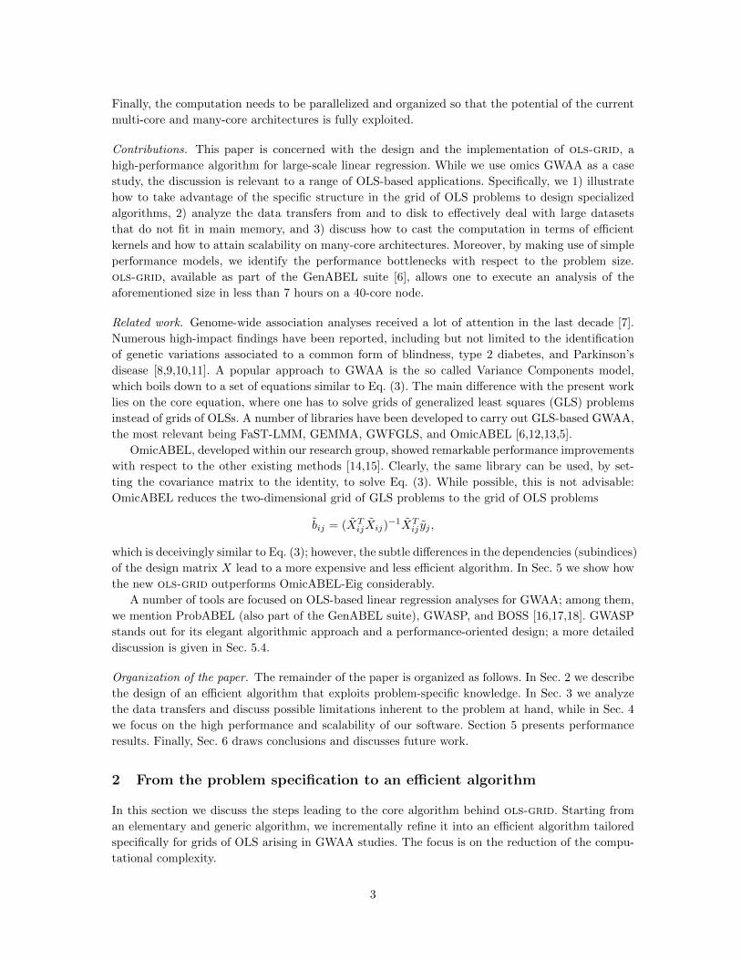
Algorithm 1 : Structure of X exposed and exploited
1: {QL, RTL} := qr(XL) (qr) 2nl2
2: for i := 1 to m do
3: RTRi := QTLXRi
(gemm) 2mlnr4: Ti := XRi −QLRTRi (gemm) 2mlnr5: {QRi , RBRi} := qr(Ti) (qr) 2mnr2
6: for j := 1 to t do
7: zij :=
(QT
L
QTRi
)yj (gemv) 2mtpn
8: bj :=
(RTL RTRi
0 RBRi
)−1
zij (trsv) mtp2
9: end for
10: end for
which can be rewritten as (RTLbT +RTRibB = zTj
RBRibB = zBij
).
Straightforward manipulation suffices to show that bT and bB can be computed as
bBij:= R−1
BRizBij
bTij := R−1TL(zTj −RTRibBij ). (6)
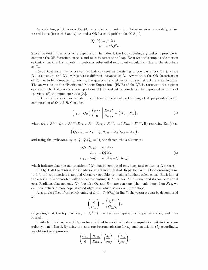
Given the dependencies with the loop indices, the top part of b can be partially precomputed by
first moving the operation kj := R−1TLzTij to the same initial loop where zTj := QT
Lyj is precomputed,
and then moving the operation hi := R−1TLRTRi out of the innermost loop. The resulting algorithm
is displayed in Alg. 2. As discussed, zTjand kj are precomputed in an initial loop (lines 2–5), and
kj is kept in memory (a few megabytes at most) for later use within the nested double-loop (line
14). Also, the computation of hi is taken out of the innermost loop (line 10) and reused within the
innermost loop (line 14). The cost of Alg. 2 is dominated by the term 2mtrn, that is, a factor of
p/r fewer operations with respect to Alg. 1.
3 Out-of-core algorithm: Analysis of data streaming
As mentioned in Sec. 1, the second challenge to be addressed when dealing with series and grids of
least squares problems is the management of large datasets. An example clarifies the situation; in
the characteristic scenario in which n = 30,000, p = 10 (r = 2), m = 107, and t = 104, the input
dataset is of size 2.4 TBs, and the computation generates 4 TBs as output. Since such datasets
exceed the main memory capacity of current shared-memory nodes and therefore reside on disk, one
has to resort to an out-of-core algorithm [21]. The main idea behind our design is to effectively tile
(block) the computation to amortize the time spent in moving data.
To emphasize the need for tiling, we commence by discussing the I/O requirements of a naive
out-of-core implementation of Alg. 2, as sketched in Alg. 3. First, the algorithm requires the loading
of the entire set of vectors yj (line 2) for the computations in the initial loop. Then, it loads once
the entire set of matrices XRi(line 6), loads m times the entire set of vectors yj (line 9), and finally
requires the storage of the resulting m × t vectors bij (line 11). The reading of yj for a total of m
times (line 9) is the clear I/O bottleneck. For the aforementioned example, the algorithm generates
12 petabytes of disk-to-memory traffic, which at a (rather optimistic) transfer rate of 2 GBytes/sec,
5
Algorithm 2 : Structure of Q and R exposed and exploited
1: {QL, RTL} := qr(XL) (qr) 2nl2
2: for j := 1 to t do
3: zTj := QTLyj (gemv) 2tln
4: kj := R−1TLzTj (trsv) tl2
5: end for
6: for i := 1 to m do
7: RTRi := QTLXRi
(gemm) 2mlnr8: Ti := XRi −QLRTRi (gemm) 2mlnr9: {QRi , RBRi} := qr(Ti) (qr) 2mnr2
10: hi := R−1TLRTRi
(trsm) ml2r11: for j := 1 to t do
12: zBij := QTRiyj (gemv) 2mtrn
13: bBij := R−1BRi
zBij (trsv) mtr2
14: bTij := kj − hibBij (gemv) 2mtlr15: end for
16: end for
would take 70 days of I/O. It is thus imperative to reorganize I/O and computation to greatly reduce
the amount of generated I/O traffic.
Algorithm 3 : Naive out-of-core approach1: Load matrix XL 4ln→ < 1 MBs
2: for j := 1 to t do
3: Load vector yj 4tn→ 1.2 GBs
4: Compute with yj
5: end for
6: for i := 1 to m do
7: Load matrix XRi 4mnr → 2.4 TBs
8: Compute with XRi
9: for j := 1 to t do
10: Load vector yj 4mtn→ 12 PBs
11: Compute with XRi , yj
12: Store vector βij 4mtp→ 4 TBs
13: end for
14: end for
3.1 Analysis of computational cost over data movement
A tiled algorithm decomposes the computation of the 2D grid of problems into subgrids or tiles.
Instead of loading one single matrix XRiand vector yj , and storing one single vector bij , the idea
is to load and store multiple of them in a slab. The tiled algorithm presented in Alg. 4 loads slabs
of tb vectors yj (Y ) and mb matrices XRi(XR) in lines 4, 11, and 19; and stores slabs of computed
mb × tb vectors bij (B) in line 27.
With tiling, the amount of I/O required by line 19 of Alg. 4 is constrained to
t× n× m
mb,
6
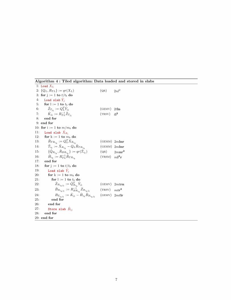
Algorithm 4 : Tiled algorithm: Data loaded and stored in slabs1: Load XL
2: {QL, RTL} := qr(XL) (qr) 2nl2
3: for j := 1 to t/tb do
4: Load slab Yj
5: for l := 1 to tb do
6: ZTjl:= QT
LYjl (gemv) 2tln
7: Kjl := R−1TLZTjl
(trsv) tl2
8: end for
9: end for
10: for i := 1 to m/mb do
11: Load slab XRi
12: for k := 1 to mb do
13: RTRik:= QT
LXRik(gemm) 2mlnr
14: Tik := XRik−QLRTRik
(gemm) 2mlnr
15: {QRik, RBRik
} := qr(Tik ) (qr) 2mnr2
16: Hik := R−1TLRTRik
(trsm) ml2r17: end for
18: for j := 1 to t/tb do
19: Load slab Yj
20: for k := 1 to mb do
21: for l := 1 to tb do
22: ZBikjl:= QT
RikYjl (gemv) 2mtrn
23: BBikjl:= R−1
BRikZBikjl
(trsv) mtr2
24: BTikjl:= Kjl − Hik BBikjl
(gemv) 2mtlr25: end for
26: end for
27: Store slab Bij
28: end for
29: end for
7
and, most importantly, can be adjusted by setting the parameter mb. We note that, in terms of
I/O overhead, there is no need to set mb to the largest possible value allowed by the available main
memory: it suffices to choose mb large enough so that the I/O bottleneck shifts to the loading of
XR and writing of B:
t× n× m
mb� m× n× r +m× t× p.
After choosing a sufficiently large value for mb, the ratio of computation over data movement is
O(mtrn)
O(mnr +mtp)≡ O(trn)
O(nr + tp). (7)
Therefore, beyond the freedom in parameterizing mb, it is the actual instance of the equation, that
is, the problem sizes, which determines whether the computation is compute-bound or IO-bound.
We illustrate the different scenarios (memory-bound vs IO-bound) in Sec. 5, where we present
experimental results.
3.2 Overlapping I/O with computation: double buffering
For problems that are not largely dominated by I/O, it is possible to reduce or even completely elim-
inate the overhead due to I/O operations by overlapping I/O with computation. In the development
of ols-grid, we adopted the well-known double buffering mechanism to asynchronously load and
store data: the main memory is logically split into two buffers; while operations within an iteration
of the innermost loop are performed on the slabs previously loaded in one of the buffers, a dedicated
I/O thread operating on the other buffer downloads the results of the previous iteration and uploads
the slabs for the next one. The experiments in Sec. 5 confirm that this mechanism mitigates the
negative effect of data transfers and, for compute-bound scenarios, it prevents I/O from limiting the
scalability of our solver.
4 High performance and scalability
In the previous sections, we designed an algorithm that avoids redundant computations, and studied
the impact of data transfers to constrain (or even eliminate) the overhead due to I/O. One last issue
remains to be addressed: how to exploit shared-memory parallelism. In this section, we illustrate
how to reorganize the computation so that it can be cast in terms of efficient BLAS-3 operations,
and discuss how to combine different types of parallelism to attain scalability.
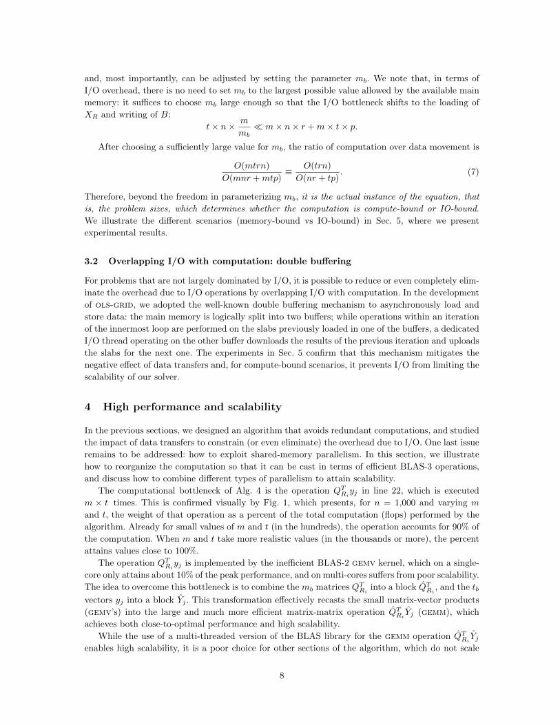
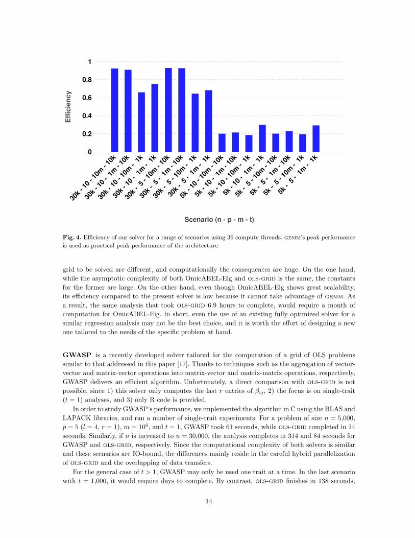
The computational bottleneck of Alg. 4 is the operation QTRiyj in line 22, which is executed
m × t times. This is confirmed visually by Fig. 1, which presents, for n = 1,000 and varying m
and t, the weight of that operation as a percent of the total computation (flops) performed by the
algorithm. Already for small values of m and t (in the hundreds), the operation accounts for 90% of
the computation. When m and t take more realistic values (in the thousands or more), the percent
attains values close to 100%.
The operation QTRiyj is implemented by the inefficient BLAS-2 gemv kernel, which on a single-
core only attains about 10% of the peak performance, and on multi-cores suffers from poor scalability.
The idea to overcome this bottleneck is to combine the mb matrices QTRi
into a block QTRi
, and the tb
vectors yj into a block Yj . This transformation effectively recasts the small matrix-vector products
(gemv’s) into the large and much more efficient matrix-matrix operation QTRiYj (gemm), which
achieves both close-to-optimal performance and high scalability.
While the use of a multi-threaded version of the BLAS library for the gemm operation QTRiYj
enables high scalability, it is a poor choice for other sections of the algorithm, which do not scale
8
104
Number of matrices X Ri
(m)10
3
102
10110
1
102
Number of vectors yj (t)
103
40%
50%
60%
70%
80%
90%
100%
104
50%
60%
70%
80%
90%
Fig. 1. Percentage of the computation performed by the operation QTRiyj from the total operations required
by Algorithm 4.
as nicely. In fact, when using a large number of cores (as is the case in our experiments), the
weight of these other sections increases to the point that it affects the overall scalability. As a
solution to mitigate this problem we turn to a hybrid parallelism combining multi-threaded BLAS
with OpenMP. Lines 13, 14, and 16 in Alg. 4 are examples of operations that do not scale with
a mere use of a multi-threaded BLAS. Let us illustrate the issue with the matrix product in line
13. One of these gemm’s in isolation multiplies QTL ∈ Rl×n with XRi ∈ Rn×r; that is, it multiplies
a wide matrix with only a few rows times a thin matrix with only a few columns. Even when mb
XRi’s are combined into the block XRi
, one of the matrices (QL) is still rather small. In terms of
number of operations per element, the ratio is very low, which results in an inefficient and poorly
scalable operation. In this case, using a multi-threaded BLAS is not sufficient (in our experiments we
observed a performance of about 5 GF/s, i.e., below 1% efficiency). Instead, we decide to explicitly
split the operation among the compute threads by means of OpenMP directives. Each thread takes
a proportional number of columns from XRi and computes the corresponding gemm using a single-
threaded BLAS call. This second alternative results in a speedup of 5x to 10x, sufficient to mitigate
the impact in the overall performance and scalability.
The resulting algorithm is displayed in Alg. 5. Among the computational bottlenecks, we high-
light in green the operations parallelized by means of a multi-threaded version of BLAS (line 18)
and in blue the operations parallelized using OpenMP (lines 10–12). As we show in the next sec-
tion, the recasting of small operations into larger ones and the use of a hybrid form of parallelism
that combines multi-threaded BLAS and OpenMP leads to satisfactory performance and scalability
signatures.
9
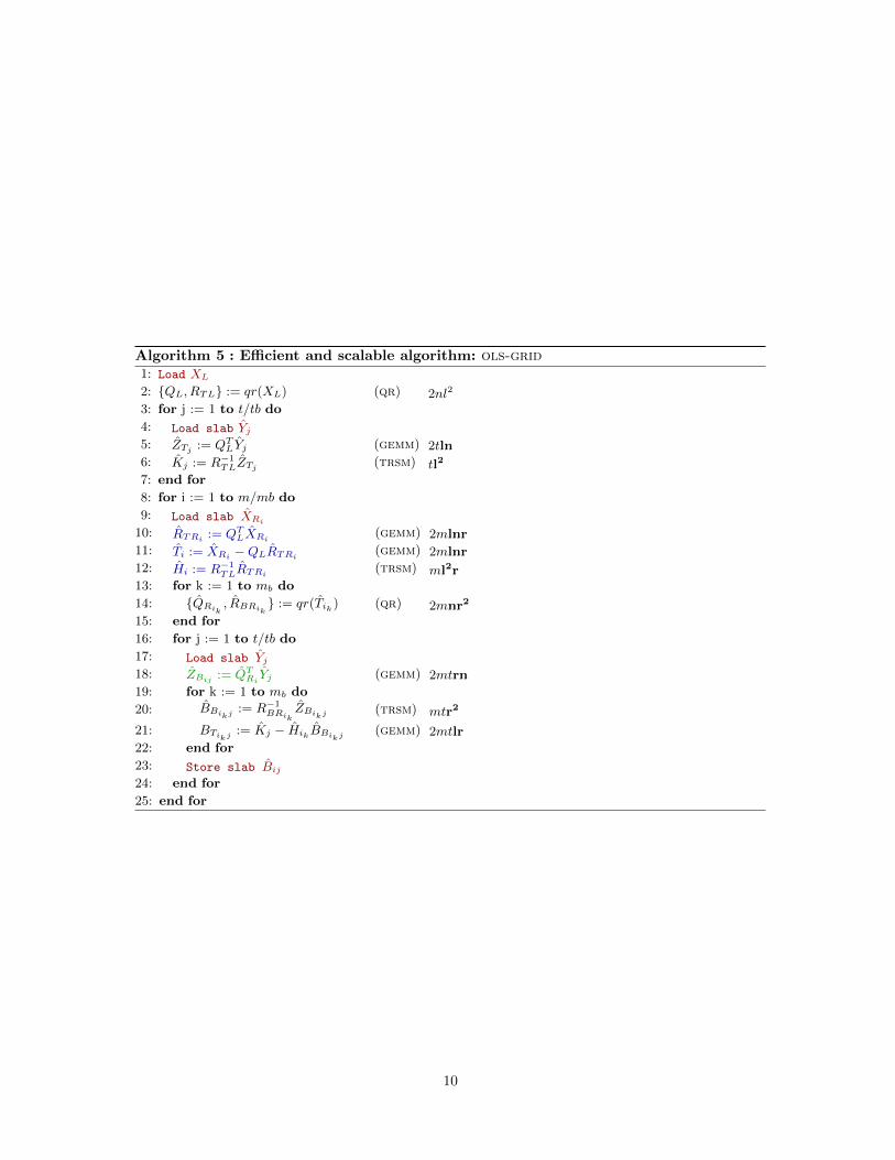
Algorithm 5 : Efficient and scalable algorithm: ols-grid1: Load XL
2: {QL, RTL} := qr(XL) (qr) 2nl2
3: for j := 1 to t/tb do
4: Load slab Yj
5: ZTj := QTLYj (gemm) 2tln
6: Kj := R−1TLZTj
(trsm) tl2
7: end for
8: for i := 1 to m/mb do
9: Load slab XRi
10: RTRi := QTLXRi
(gemm) 2mlnr11: Ti := XRi −QLRTRi
(gemm) 2mlnr12: Hi := R−1
TLRTRi(trsm) ml2r
13: for k := 1 to mb do
14: {QRik, RBRik
} := qr(Tik ) (qr) 2mnr2
15: end for
16: for j := 1 to t/tb do
17: Load slab Yj
18: ZBij := QTRiYj (gemm) 2mtrn
19: for k := 1 to mb do
20: BBikj := R−1BRik
ZBikj (trsm) mtr2
21: BTikj := Kj − Hik BBikj (gemm) 2mtlr22: end for
23: Store slab Bij
24: end for
25: end for
10
5 Experimental results
In this section, ols-grid (the implementation of Alg. 5) is tested in a variety of settings to provide
evidence that it makes a nearly optimal use of the available resources; it is also compared and
contrasted with a number of available alternatives, namely a naive solver (the linear regression
solver from ProbABEL), a specialized solver for grids of GLS (generalized least squares) problems
(OmicABEL-Eig), and a specialized solver for grids of OLS problems (GWASP).
All our tests were run on a system consisting of 4 Intel(R) Xeon(R) E7-4850 Westmere-EX
multi-core processors. Each processor comprises 10 cores operating at a frequency of 2.00 GHz,
for a combined peak performance in single precision of 640 GFlops/sec. The system is equipped
with 256 GBs of RAM and 8 TBs of disk as secondary memory; our measurements indicate that
the Lustre file system attains a maximum bandwidth of about 300 MBs/sec and 1.7 GBs/sec for
writing and reading operations, respectively. The solver was compiled using Intel’s icc compiler
(v14.0.1), and linked to Intel’s MKL multi-threaded library (v14.0.1), which provides for BLAS and
LAPACK functionality. The routine makes use of the OpenMP parallelism provided by the compiler
through a number of pragma directives. All computations were performed in single precision, and
the correctness of the results was assessed by direct comparison with the OLS solver from LAPACK
(sgels).
For the asynchronous I/O transfers, we initially tested the AIO library (available in all Unix
systems). We observed that I/O operations had a considerable impact in performance by limiting
the flops attained by gemm. Since AIO does not offer the means to specify the amount of threads
spawned for I/O and to pin threads to cores, we developed our own light-weight library which uses
one single thread for I/O operations and allows thread pinning.3
5.1 Compute-bound vs IO-bound scenarios
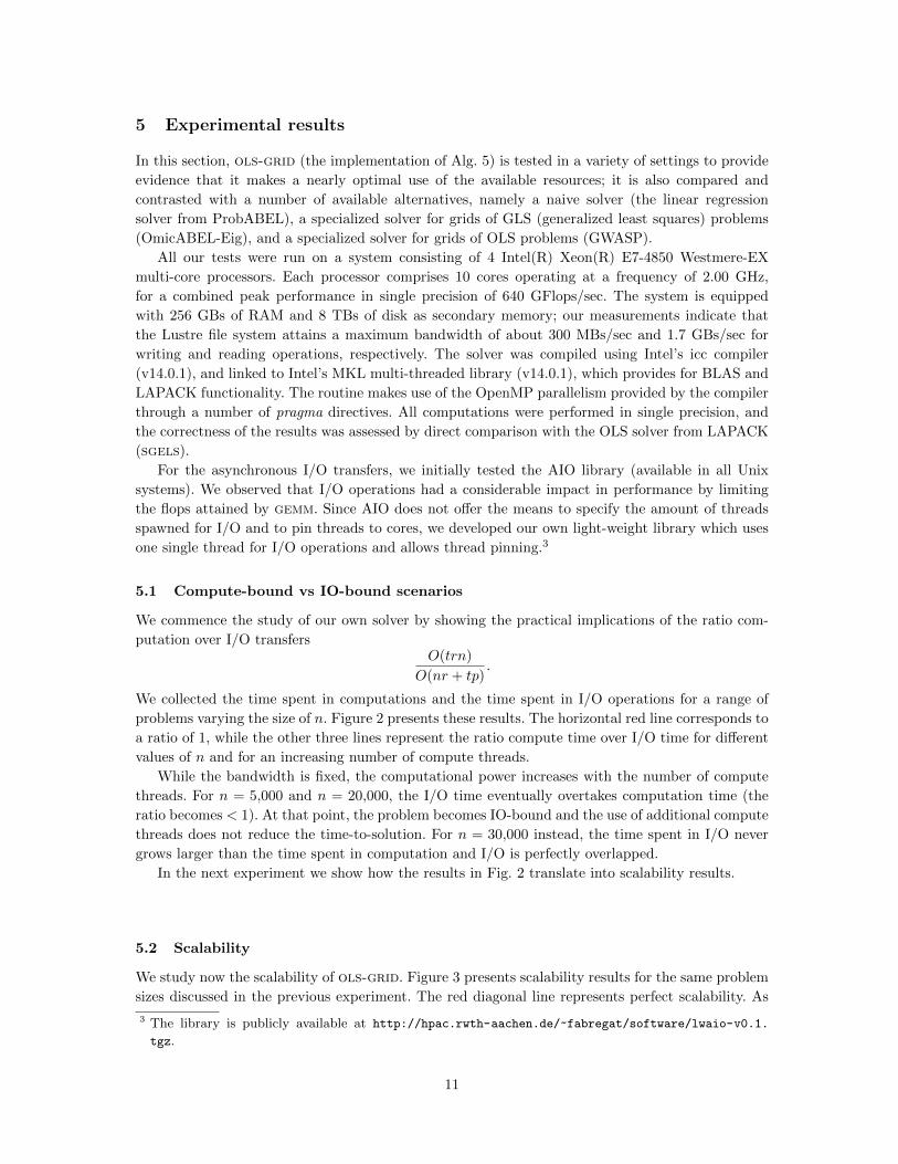
We commence the study of our own solver by showing the practical implications of the ratio com-
putation over I/O transfersO(trn)
O(nr + tp).
We collected the time spent in computations and the time spent in I/O operations for a range of
problems varying the size of n. Figure 2 presents these results. The horizontal red line corresponds to
a ratio of 1, while the other three lines represent the ratio compute time over I/O time for different
values of n and for an increasing number of compute threads.
While the bandwidth is fixed, the computational power increases with the number of compute
threads. For n = 5,000 and n = 20,000, the I/O time eventually overtakes computation time (the
ratio becomes < 1). At that point, the problem becomes IO-bound and the use of additional compute
threads does not reduce the time-to-solution. For n = 30,000 instead, the time spent in I/O never
grows larger than the time spent in computation and I/O is perfectly overlapped.
In the next experiment we show how the results in Fig. 2 translate into scalability results.
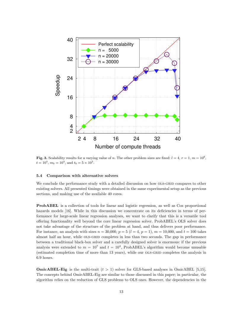
5.2 Scalability
We study now the scalability of ols-grid. Figure 3 presents scalability results for the same problem
sizes discussed in the previous experiment. The red diagonal line represents perfect scalability. As
3 The library is publicly available at http://hpac.rwth-aachen.de/~fabregat/software/lwaio-v0.1.
tgz.
11
0
0.5
1
1.5
2
2.5
3
4 8 16 24 32 39
Ratio (
Com
puta
tion tim
e / IO
tim
e)
Number of compute threads
n = 5000
n = 20000
n = 30000
Fig. 2. Ratio of compute time over I/O time. Results for a varying value of n and an increasing number
of compute threads. The other problem sizes are fixed: l = 4, r = 1, m = 106, t = 104, mb = 104, and
tb = 5× 10³.
the ratio in Fig. 2 suggested, the line for n = 5,000 shows perfect scalability for up to 8 threads; from
that point on, the I/O transfers dominate the execution time and no larger speedups are possible.
Similarly, for n = 20,000, almost perfect scalability is attained with up to 28 compute threads. Again,
beyond that number, the I/O dominates and the scalability plateaus. Instead, for n = 30,000, the
I/O never dominates execution time and the solver attains speedups of around 34x when 36 compute
threads are used. In all cases, we observe a drop in scalability when 40 compute threads are used;
this is because one compute thread and the I/O thread share one core. We attribute the drop at
39 compute threads for the experiment with n = 30,000—and, less apparently, at n = 5,000 and
n = 20,000—to potential memory conflicts, since in the used architecture each pair of threads share
the L1 and L2 caches.
An important message to extract from these results is the need to understand the characteristics
of the problem at hand to decide which architecture fits best our needs. In the case of omics GWAA,
the size of n plays an important role in the decision of whether investing in further computational
power or larger bandwidth.
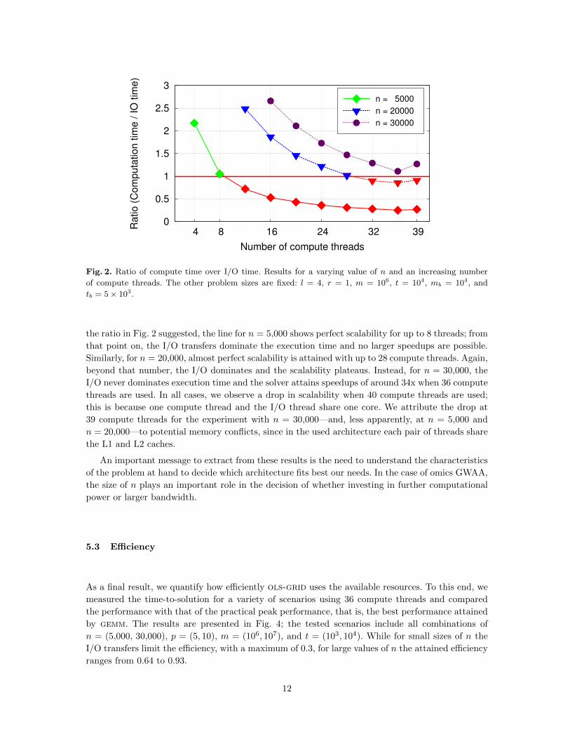
5.3 Efficiency
As a final result, we quantify how efficiently ols-grid uses the available resources. To this end, we
measured the time-to-solution for a variety of scenarios using 36 compute threads and compared
the performance with that of the practical peak performance, that is, the best performance attained
by gemm. The results are presented in Fig. 4; the tested scenarios include all combinations of
n = (5,000, 30,000), p = (5, 10), m = (106, 107), and t = (103, 104). While for small sizes of n the
I/O transfers limit the efficiency, with a maximum of 0.3, for large values of n the attained efficiency
ranges from 0.64 to 0.93.
12
2 4
8
16
24
32
40
2 4 8 16 24 32 40
Sp
ee
du
p
Number of compute threads
Perfect scalability
n = 5000
n = 20000
n = 30000
Fig. 3. Scalability results for a varying value of n. The other problem sizes are fixed: l = 4, r = 1, m = 106,
t = 104, mb = 104, and tb = 5× 10³.
5.4 Comparison with alternative solvers
We conclude the performance study with a detailed discussion on how ols-grid compares to other
existing solvers. All presented timings were obtained in the same experimental setup as the previous
sections, and making use of the available 40 cores.
ProbABEL is a collection of tools for linear and logistic regression, as well as Cox proportional
hazards models [16]. While in this discussion we concentrate on its deficiencies in terms of per-
formance for large-scale linear regression analyses, we want to clarify that this is a versatile tool
offering functionality well beyond the core linear regression solver. ProbABEL’s OLS solver does
not take advantage of the structure of the problem at hand, and thus delivers poor performance.
For instance, an analysis with sizes n = 30,000, p = 5 (l = 4, p = 1), m = 10,000, and t = 100 takes
almost half an hour, while ols-grid completes in less than two seconds. The gap in performance
between a traditional black-box solver and a carefully designed solver is enormous: if the previous
analysis were extended to m = 107 and t = 104, ProbABEL’s algorithm would become unusable
(estimated completion time of more than 13 years), while our ols-grid completes the analysis in
6.9 hours.
OmicABEL-Eig is the multi-trait (t > 1) solver for GLS-based analyses in OmicABEL [5,15].
The concepts behind OmicABEL-Eig are similar to those discussed in this paper; in particular, the
algorithm relies on the reduction of GLS problems to OLS ones. However, the dependencies in the
13
0
0.2
0.4
0.6
0.8
1
30k
- 10
- 10m
- 10
k
30k
- 10
- 1m
- 10
k
30k
- 10
- 10m
- 1
k
30k
- 10
- 1m
- 1
k
30k
- 5
- 10m
- 10
k
30k
- 5
- 1m
- 10
k
30k
- 5
- 10m
- 1
k
30k
- 5
- 1m
- 1
k
5k
- 10
- 10m
- 10
k
5k
- 10
- 1m
- 10
k
5k
- 10
- 10m
- 1
k
5k
- 10
- 1m
- 1
k
5k
- 5
- 10m
- 10
k
5k
- 5
- 1m
- 10
k
5k
- 5
- 10m
- 1
k
5k
- 5
- 1m
- 1
k
Eff
icie
ncy
Scenario (n - p - m - t)
Fig. 4. Efficiency of our solver for a range of scenarios using 36 compute threads. gemm’s peak performance
is used as practical peak performance of the architecture.
grid to be solved are different, and computationally the consequences are huge. On the one hand,
while the asymptotic complexity of both OmicABEL-Eig and ols-grid is the same, the constants
for the former are large. On the other hand, even though OmicABEL-Eig shows great scalability,
its efficiency compared to the present solver is low because it cannot take advantage of gemm. As
a result, the same analysis that took ols-grid 6.9 hours to complete, would require a month of
computation for OmicABEL-Eig. In short, even the use of an existing fully optimized solver for a
similar regression analysis may not be the best choice, and it is worth the effort of designing a new
one tailored to the needs of the specific problem at hand.
GWASP is a recently developed solver tailored for the computation of a grid of OLS problems
similar to that addressed in this paper [17]. Thanks to techniques such as the aggregation of vector-
vector and matrix-vector operations into matrix-vector and matrix-matrix operations, respectively,
GWASP delivers an efficient algorithm. Unfortunately, a direct comparison with ols-grid is not
possible, since 1) this solver only computes the last r entries of βij , 2) the focus is on single-trait
(t = 1) analyses, and 3) only R code is provided.
In order to study GWASP’s performance, we implemented the algorithm in C using the BLAS and
LAPACK libraries, and ran a number of single-trait experiments. For a problem of size n = 5,000,
p = 5 (l = 4, r = 1), m = 106, and t = 1, GWASP took 61 seconds, while ols-grid completed in 14
seconds. Similarly, if n is increased to n = 30,000, the analysis completes in 314 and 84 seconds for
GWASP and ols-grid, respectively. Since the computational complexity of both solvers is similar
and these scenarios are IO-bound, the differences mainly reside in the careful hybrid parallelization
of ols-grid and the overlapping of data transfers.
For the general case of t > 1, GWASP may only be used one trait at a time. In the last scenario
with t = 1,000, it would require days to complete. By contrast, ols-grid finishes in 138 seconds,
14
thanks to the optimizations enabled when considering the 2D grid of problems as a whole. Despite
this relatively large gap, we believe that GWASP can be extended to multi-trait analyses and to the
computation of entire β’s, while achieving performance comparable to that of our solver.
6 Conclusions
We addressed the design and implementation of efficient solvers for large-scale linear regression
analyses. As case study, we focused on the computation of a two-dimensional grid of ordinary least
squares problems as it appears in the context of genome-wide association analyses. The resulting
routine, ols-grid, showed to be highly efficient and scalable.
Starting from the mathematical description of the problem, we designed an incore algorithm
that exploits the available problem-specific knowledge and structure. Next, to enable the solution of
problems with large datasets that do not fit in today multi-core’s main memory, we transformed the
incore algorithm into an out-of-core one, which, thanks to tiling, constrains the amount of required
data movement. By incorporating the double-buffering technique and using an asynchronous I/O
library, we completely eliminated I/O overhead whenever possible.
Finally, by reorganizing the calculations, the computational bottleneck was cast in terms of the
highly efficient gemm routine. Combining multi-threaded BLAS and OpenMP parallelism, ols-grid
also attains high performance and high scalability. More specifically, for large enough analyses, the
solver achieves single-core efficiency beyond 90% of peak performance, and speedups of up to 34x
with 36 cores.
While previously existing tools allow for multiple trait analysis, these are limited to small datasets
and require considerable runtimes. We enable the analysis of previously intractable datasets and offer
shorter times to solution. Our ols-grid solver is already integrated in the GenABEL suite, and
adopted by a number of research groups.
6.1 Future work
Two main research directions remain open. On the one hand, support for distributed-memory ar-
chitectures is desirable, allowing for further reduction in time-to-solution. This step will require a
careful distribution of workload among nodes and the use of advanced I/O techniques to prevent
data movement from becoming a bottleneck.
On the other hand, we are already working on the support for so-called missing and erroneous
data. Often, large datasets are collected by combining data from different sources. Therefore, subsets
of data for certain individuals (for instance, entries in yj vectors) may not be available and labeled
as missing values (NaNs). Erroneous data may origin, for instance, from errors in the acquisition.
Accepting input data with NaN values (and preprocessing it accordingly) will make our software of
broader appeal and will facilitate its adoption by the broad GWAA community.
Acknowledgments
Financial support from the Deutsche Forschungsgemeinschaft (German Research Association)
through grant GSC 111 is gratefully acknowledged. The authors thank Yurii Aulchenko for fruitful
discussions on the biological background of GWAA.
References
1. L. A. Hindorff, P. Sethupathy, H. A. Junkins, E. M. Ramos, J. P. Mehta, F. S. Collins, T. A. Manolio,
Potential etiologic and functional implications of genome-wide association loci for human diseases and
traits, Proc. Natl. Acad Sci. USA 106 (23) (2009) 9362–9367. doi:10.1073/pnas.0903103106.
15
2. X. Sala-I-Martin, I just ran two million regressions, The American Economic Review 87 (2) (1997)
178–183.
3. C. Gieger, L. Geistlinger, E. Altmaier, M. Hrabe de Angelis, F. Kronenberg, T. Meitinger, H.-W. W.
Mewes, H.-E. E. Wichmann, K. M. Weinberger, J. Adamski, T. Illig, K. Suhre, Genetics meets
metabolomics: a genome-wide association study of metabolite profiles in human serum., PLoS Genet
4 (11) (2008) e1000282+.
4. A. Demirkan, C. M. Van Duijn, P. Ugocsai, A. Isaacs, P. P. Pramstaller, G. Liebisch, J. F. Wilson, . Jo-
hansson, I. Rudan, Y. S. Aulchenko, et al., Genome-wide association study identifies novel loci associated
with circulating phospho- and sphingolipid concentrations., PLoS Genetics 8 (2) (2012) e1002490.
5. D. Fabregat-Traver, S. Sharapov, C. Hayward, I. Rudan, H. Campbell, Y. Aulchenko, P. Bientinesi,
Big-Data, High-Performance, Mixed Models Based Genome-Wide Association Analysis with omicABEL
software, F1000Research 3 (200).
6. Y. S. Aulchenko, S. Ripke, A. Isaacs, C. M. van Duijn, Genabel: an R library for genome-wide association
analysis., Bioinformatics 23 (10) (2007) 1294–6.
7. L. Hindorff, J. MacArthur, A. Wise, H. Junkins, P. Hall, A. Klemm, T. Manolio, A catalog of published
genome-wide association studies, available at: www.genome.gov/gwastudies. Accessed April 12th (2015).
8. G. S. Hageman, et al., A common haplotype in the complement regulatory gene factor H (HF1/CFH)
predisposes individuals to age-related macular degeneration, Proc. Natl. Acad Sci. USA 102 (20) (2005)
7227–7232.
9. A. O. Edwards, R. Ritter, K. J. Abel, A. Manning, C. Panhuysen, L. A. Farrer, Complement factor H
polymorphism and age-related macular degeneration, Science 308 (5720) (2005) 421–424.
10. T. M. Frayling, Genome-wide association studies provide new insights into type 2 diabetes aetiology,
Nat Rev Genet 8 (9) (2007) 657–662.
11. M. A. Nalls, et al., Large-scale meta-analysis of genome-wide association data identifies six new risk loci
for Parkinson’s disease, Nat Genet 46 (9) (2014) 989–993, letter.
12. C. Lippert, J. Listgarten, Y. Liu, C. M. Kadie, R. I. Davidson, D. Heckerman, Fast linear mixed models
for genome-wide association studies, Nat. Methods 8 (10) (2011) 833–835.
13. X. Zhou, M. Stephens, Genome-wide efficient mixed-model analysis for association studies, Nat. Genet.
44 (7) (2012) 821–824.
14. D. Fabregat-Traver, Y. S. Aulchenko, P. Bientinesi, Solving sequences of generalized least-squares prob-
lems on multi-threaded architectures, Applied Mathematics and Computation (AMC) 234 (2014) 606–
617.
15. D. Fabregat-Traver, P. Bientinesi, Computing petaflops over terabytes of data: The case of genome-wide
association studies, ACM Trans. Math. Software 40 (4) (2014) 27:1–27:22.
16. Y. S. Aulchenko, M. V. Struchalin, C. M. van Duijn, ProbABEL package for genome-wide association
analysis of imputed data, BMC Bioinformatics 11 (2010) 134.
17. K. Sikorska, E. Lesaffre, P. F. J. Groenen, P. H. C. Eilers, GWAS on your notebook: fast semi-parallel
linear and logistic regression for genome-wide association studies, BMC Bioinformatics 14 (2013) 166.
18. A. Voorman, K. Rice, T. Lumley, Fast computation for genome-wide association studies using boosted
one-step statistics, Bioinformatics 28 (14) (2012) 1818–1822.
19. G. H. Golub, C. F. Van Loan, Matrix computations (3rd ed.), Johns Hopkins University Press, Baltimore,
MD, USA, 1996.
20. D. Fabregat-Traver, P. Bientinesi, Knowledge-based automatic generation of Partitioned Matrix Expres-
sions, in: Computer Algebra in Scientific Computing, Vol. 6885 of Lecture Notes in Computer Science,
Springer Berlin Heidelberg, 2011, pp. 144–157.
21. S. Toledo, External memory algorithms, American Mathematical Society, Boston, MA, USA, 1999, Ch.
A survey of out-of-core algorithms in numerical linear algebra, pp. 161–179.
16