Embed Size (px)
Citation preview

Large-scale machine learningand convex optimization
Francis Bach
INRIA - Ecole Normale Superieure, Paris, France
Allerton Conference - September 2015
Slides available at www.di.ens.fr/~fbach/gradsto_allerton.pdf
Context
Machine learning for “big data”
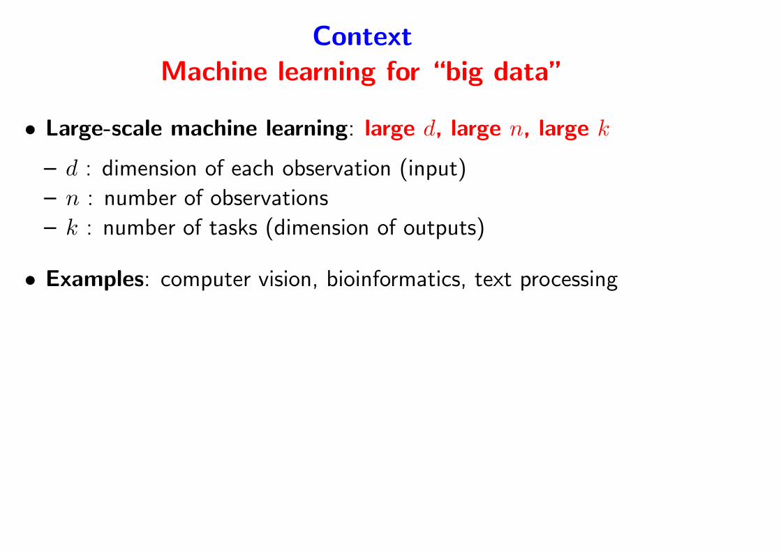
• Large-scale machine learning: large d, large n, large k
– d : dimension of each observation (input)
– n : number of observations
– k : number of tasks (dimension of outputs)
• Examples: computer vision, bioinformatics, text processing
– Ideal running-time complexity: O(dn+ kn)
– Going back to simple methods
– Stochastic gradient methods (Robbins and Monro, 1951)
– Mixing statistics and optimization
– Using smoothness to go beyond stochastic gradient descent
Visual object recognition

Personal photos
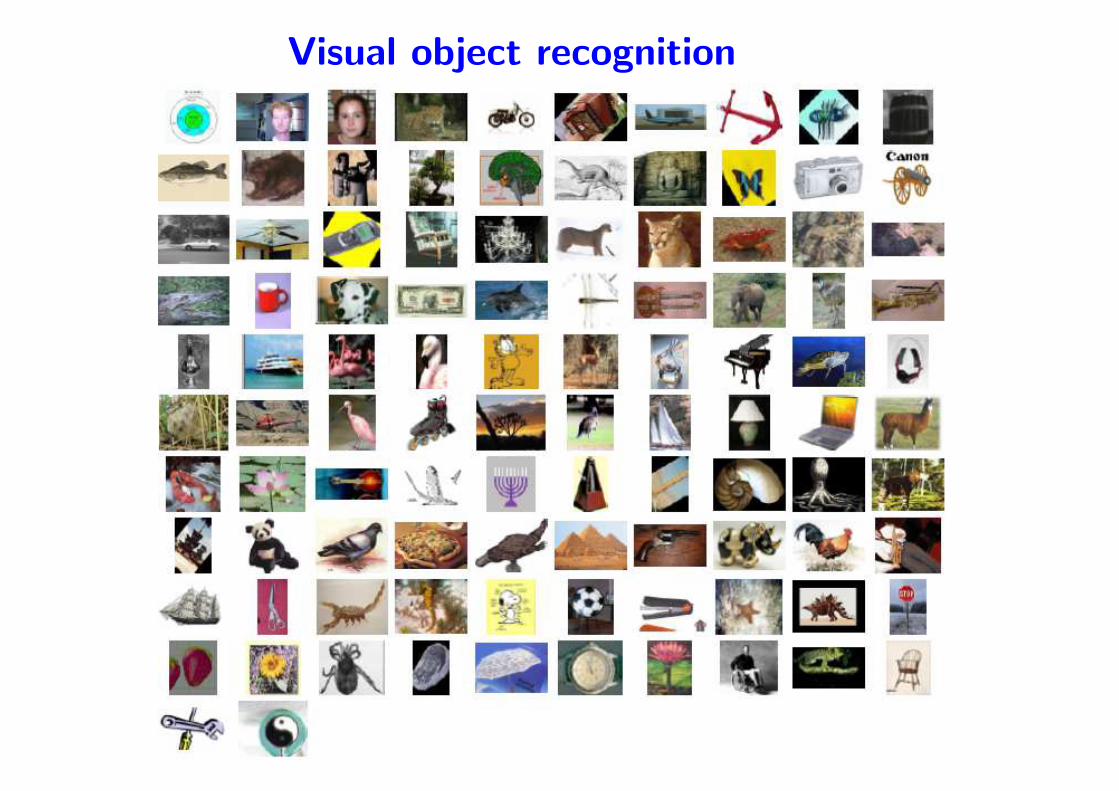
Learning for bioinformatics - Proteins
• Crucial components of cell life
• Predicting multiple functions and
interactions
• Massive data: up to 1 millions for
humans!
• Complex data
– Amino-acid sequence
– Link with DNA
– Tri-dimensional molecule

Search engines - advertising
Context
Machine learning for “big data”
• Large-scale machine learning: large d, large n, large k
– d : dimension of each observation (input)
– n : number of observations
– k : number of tasks (dimension of outputs)
• Examples: computer vision, bioinformatics, text processing
• Ideal running-time complexity: O(dn+ kn)
– Going back to simple methods
– Stochastic gradient methods (Robbins and Monro, 1951)
– Mixing statistics and optimization
– Using smoothness to go beyond stochastic gradient descent
Context
Machine learning for “big data”
• Large-scale machine learning: large d, large n, large k
– d : dimension of each observation (input)
– n : number of observations
– k : number of tasks (dimension of outputs)
• Examples: computer vision, bioinformatics, text processing
• Ideal running-time complexity: O(dn+ kn)
• Going back to simple methods
– Stochastic gradient methods (Robbins and Monro, 1951)
– Mixing statistics and optimization
– Using smoothness to go beyond stochastic gradient descent

Outline
1. Large-scale machine learning and optimization
• Traditional statistical analysis
• Classical methods for convex optimization
2. Non-smooth stochastic approximation
• Stochastic (sub)gradient and averaging
• Non-asymptotic results and lower bounds
• Strongly convex vs. non-strongly convex
3. Smooth stochastic approximation algorithms
• Asymptotic and non-asymptotic results
• Beyond decaying step-sizes
4. Finite data sets

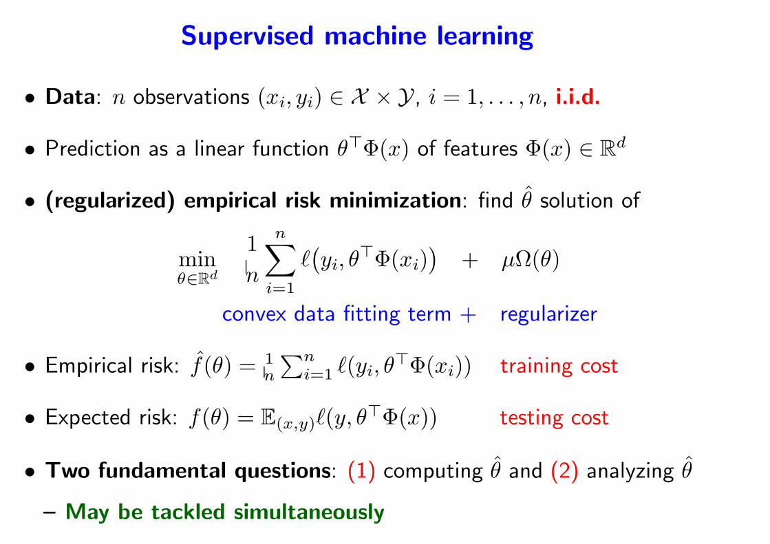
Supervised machine learning
• Data: n observations (xi, yi) ∈ X × Y, i = 1, . . . , n, i.i.d.
• Prediction as a linear function θ⊤Φ(x) of features Φ(x) ∈ Rd
• (regularized) empirical risk minimization: find θ solution of
minθ∈Rd
1
n
n∑
i=1
ℓ(
yi, θ⊤Φ(xi)
)
+ µΩ(θ)
convex data fitting term + regularizer
Usual losses
• Regression: y ∈ R, prediction y = θ⊤Φ(x)
– quadratic loss 12(y − y)2 = 1
2(y − θ⊤Φ(x))2
Usual losses
• Regression: y ∈ R, prediction y = θ⊤Φ(x)
– quadratic loss 12(y − y)2 = 1
2(y − θ⊤Φ(x))2
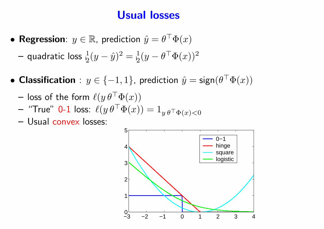
• Classification : y ∈ −1, 1, prediction y = sign(θ⊤Φ(x))
– loss of the form ℓ(y θ⊤Φ(x))– “True” 0-1 loss: ℓ(y θ⊤Φ(x)) = 1y θ⊤Φ(x)<0
– Usual convex losses:
−3 −2 −1 0 1 2 3 40
1
2
3
4
5
0−1hingesquarelogistic
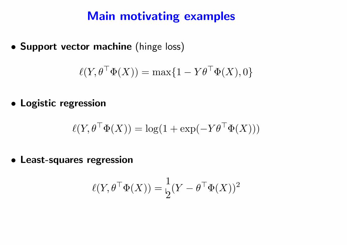
Main motivating examples
• Support vector machine (hinge loss)
ℓ(Y, θ⊤Φ(X)) = max1− Y θ⊤Φ(X), 0
• Logistic regression
ℓ(Y, θ⊤Φ(X)) = log(1 + exp(−Y θ⊤Φ(X)))
• Least-squares regression
ℓ(Y, θ⊤Φ(X)) =1
2(Y − θ⊤Φ(X))2
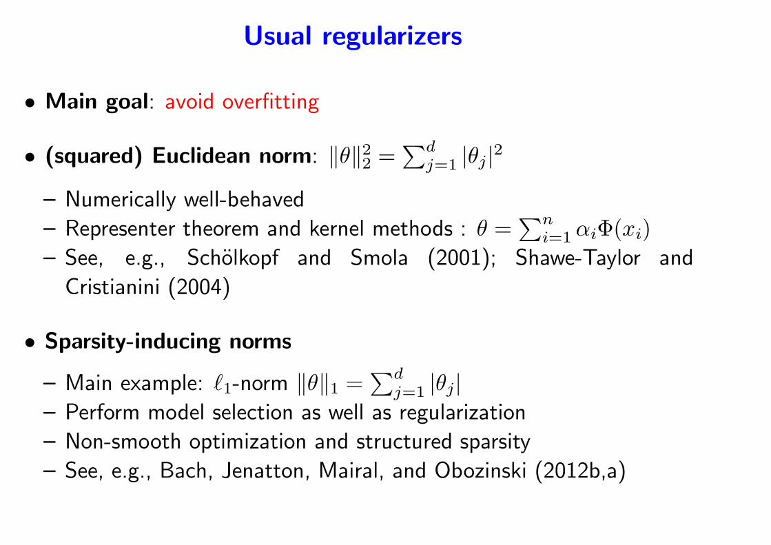
Usual regularizers
• Main goal: avoid overfitting
• (squared) Euclidean norm: ‖θ‖22 =∑d
j=1 |θj|2
– Numerically well-behaved
– Representer theorem and kernel methods : θ =∑n
i=1αiΦ(xi)
– See, e.g., Scholkopf and Smola (2001); Shawe-Taylor and
Cristianini (2004)
• Sparsity-inducing norms
– Main example: ℓ1-norm ‖θ‖1 =∑d
j=1 |θj|– Perform model selection as well as regularization
– Non-smooth optimization and structured sparsity
– See, e.g., Bach, Jenatton, Mairal, and Obozinski (2012b,a)
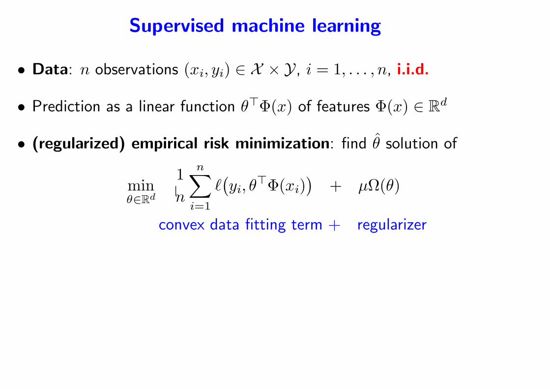
Supervised machine learning
• Data: n observations (xi, yi) ∈ X × Y, i = 1, . . . , n, i.i.d.
• Prediction as a linear function θ⊤Φ(x) of features Φ(x) ∈ Rd
• (regularized) empirical risk minimization: find θ solution of
minθ∈Rd
1
n
n∑
i=1
ℓ(
yi, θ⊤Φ(xi)
)
+ µΩ(θ)
convex data fitting term + regularizer
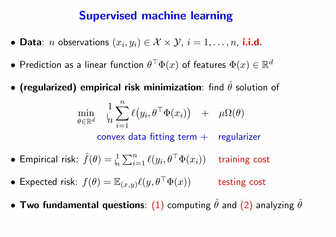
• Empirical risk: f(θ) = 1n
∑ni=1 ℓ(yi, θ
⊤Φ(xi)) training cost
• Expected risk: f(θ) = E(x,y)ℓ(y, θ⊤Φ(x)) testing cost
• Two fundamental questions: (1) computing θ and (2) analyzing θ
– May be tackled simultaneously
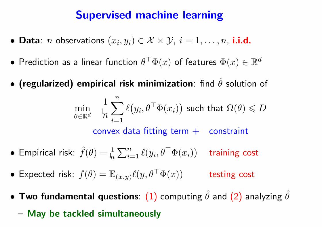
Supervised machine learning
• Data: n observations (xi, yi) ∈ X × Y, i = 1, . . . , n, i.i.d.
• Prediction as a linear function θ⊤Φ(x) of features Φ(x) ∈ Rd
• (regularized) empirical risk minimization: find θ solution of
minθ∈Rd
1
n
n∑
i=1
ℓ(
yi, θ⊤Φ(xi)
)
such that Ω(θ) 6 D
convex data fitting term + constraint
• Empirical risk: f(θ) = 1n
∑ni=1 ℓ(yi, θ
⊤Φ(xi)) training cost
• Expected risk: f(θ) = E(x,y)ℓ(y, θ⊤Φ(x)) testing cost
• Two fundamental questions: (1) computing θ and (2) analyzing θ
– May be tackled simultaneously
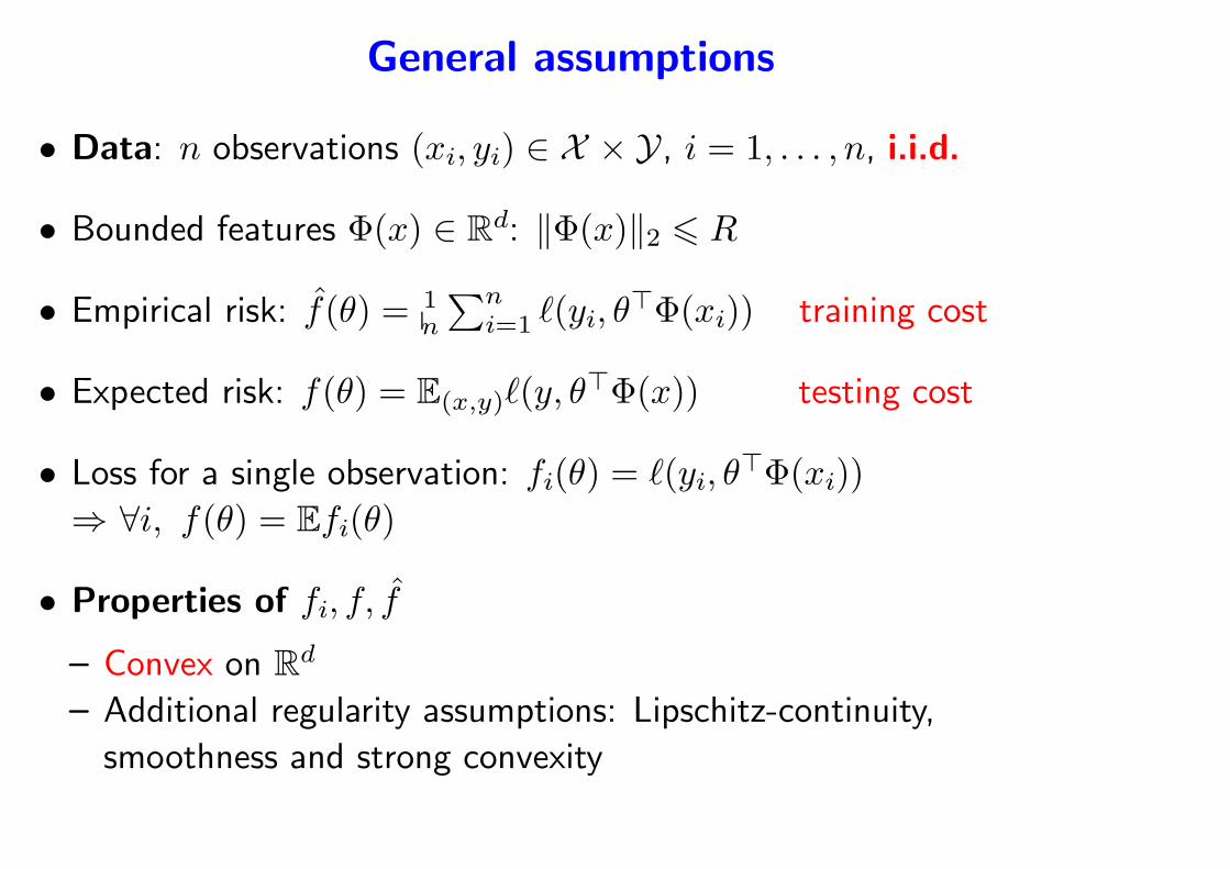
General assumptions
• Data: n observations (xi, yi) ∈ X × Y, i = 1, . . . , n, i.i.d.
• Bounded features Φ(x) ∈ Rd: ‖Φ(x)‖2 6 R
• Empirical risk: f(θ) = 1n
∑ni=1 ℓ(yi, θ
⊤Φ(xi)) training cost
• Expected risk: f(θ) = E(x,y)ℓ(y, θ⊤Φ(x)) testing cost
• Loss for a single observation: fi(θ) = ℓ(yi, θ⊤Φ(xi))
⇒ ∀i, f(θ) = Efi(θ)
• Properties of fi, f, f
– Convex on Rd
– Additional regularity assumptions: Lipschitz-continuity,
smoothness and strong convexity
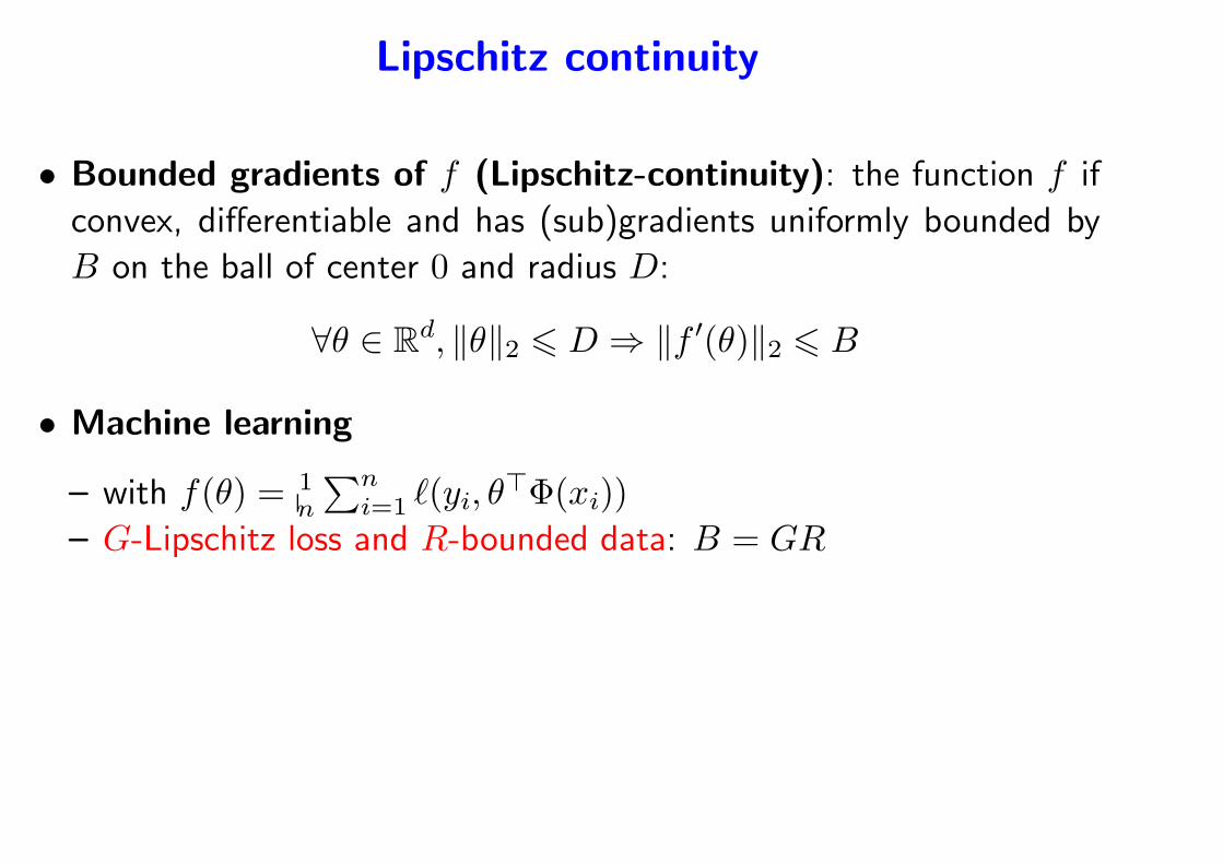
Lipschitz continuity
• Bounded gradients of f (Lipschitz-continuity): the function f if
convex, differentiable and has (sub)gradients uniformly bounded by
B on the ball of center 0 and radius D:
∀θ ∈ Rd, ‖θ‖2 6 D ⇒ ‖f ′(θ)‖2 6 B
• Machine learning
– with f(θ) = 1n
∑ni=1 ℓ(yi, θ
⊤Φ(xi))
– G-Lipschitz loss and R-bounded data: B = GR
Smoothness and strong convexity
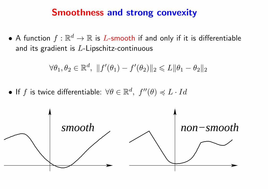
• A function f : Rd → R is L-smooth if and only if it is differentiable
and its gradient is L-Lipschitz-continuous
∀θ1, θ2 ∈ Rd, ‖f ′(θ1)− f ′(θ2)‖2 6 L‖θ1 − θ2‖2
• If f is twice differentiable: ∀θ ∈ Rd, f ′′(θ) 4 L · Id
smooth non−smooth
Smoothness and strong convexity
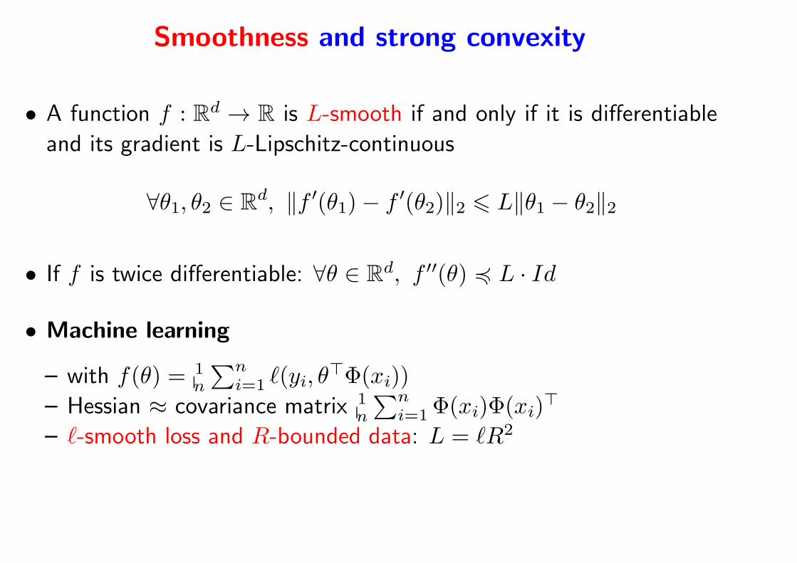
• A function f : Rd → R is L-smooth if and only if it is differentiable
and its gradient is L-Lipschitz-continuous
∀θ1, θ2 ∈ Rd, ‖f ′(θ1)− f ′(θ2)‖2 6 L‖θ1 − θ2‖2
• If f is twice differentiable: ∀θ ∈ Rd, f ′′(θ) 4 L · Id
• Machine learning
– with f(θ) = 1n
∑ni=1 ℓ(yi, θ
⊤Φ(xi))
– Hessian ≈ covariance matrix 1n
∑ni=1Φ(xi)Φ(xi)
⊤
– ℓ-smooth loss and R-bounded data: L = ℓR2
Smoothness and strong convexity
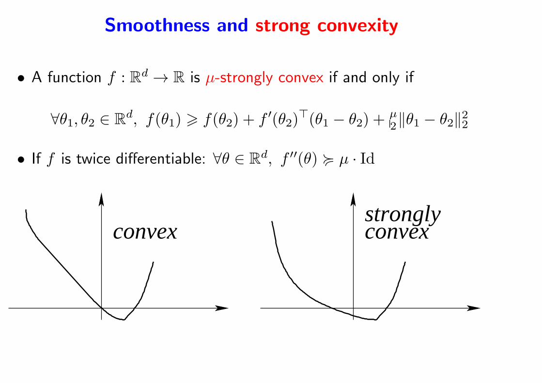
• A function f : Rd → R is µ-strongly convex if and only if
∀θ1, θ2 ∈ Rd, f(θ1) > f(θ2) + f ′(θ2)
⊤(θ1 − θ2) +µ2‖θ1 − θ2‖22
• If f is twice differentiable: ∀θ ∈ Rd, f ′′(θ) < µ · Id
convexstronglyconvex
Smoothness and strong convexity
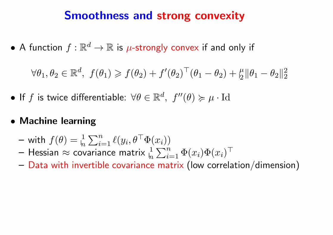
• A function f : Rd → R is µ-strongly convex if and only if
∀θ1, θ2 ∈ Rd, f(θ1) > f(θ2) + f ′(θ2)
⊤(θ1 − θ2) +µ2‖θ1 − θ2‖22
• If f is twice differentiable: ∀θ ∈ Rd, f ′′(θ) < µ · Id
• Machine learning
– with f(θ) = 1n
∑ni=1 ℓ(yi, θ
⊤Φ(xi))
– Hessian ≈ covariance matrix 1n
∑ni=1Φ(xi)Φ(xi)
⊤
– Data with invertible covariance matrix (low correlation/dimension)
Smoothness and strong convexity
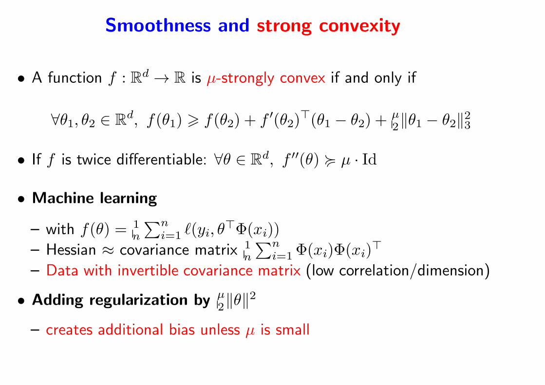
• A function f : Rd → R is µ-strongly convex if and only if
∀θ1, θ2 ∈ Rd, f(θ1) > f(θ2) + f ′(θ2)
⊤(θ1 − θ2) +µ2‖θ1 − θ2‖23
• If f is twice differentiable: ∀θ ∈ Rd, f ′′(θ) < µ · Id
• Machine learning
– with f(θ) = 1n
∑ni=1 ℓ(yi, θ
⊤Φ(xi))
– Hessian ≈ covariance matrix 1n
∑ni=1Φ(xi)Φ(xi)
⊤
– Data with invertible covariance matrix (low correlation/dimension)
• Adding regularization by µ2‖θ‖2
– creates additional bias unless µ is small

Summary of smoothness/convexity assumptions
• Bounded gradients of f (Lipschitz-continuity): the function f if
convex, differentiable and has (sub)gradients uniformly bounded by
B on the ball of center 0 and radius D:
∀θ ∈ Rd, ‖θ‖2 6 D ⇒ ‖f ′(θ)‖2 6 B
• Smoothness of f : the function f is convex, differentiable with
L-Lipschitz-continuous gradient f ′:
∀θ1, θ2 ∈ Rd, ‖f ′(θ1)− f ′(θ2)‖2 6 L‖θ1 − θ2‖2
• Strong convexity of f : The function f is strongly convex with
respect to the norm ‖ · ‖, with convexity constant µ > 0:
∀θ1, θ2 ∈ Rd, f(θ1) > f(θ2) + f ′(θ2)
⊤(θ1 − θ2) +µ2‖θ1 − θ2‖22
Analysis of empirical risk minimization
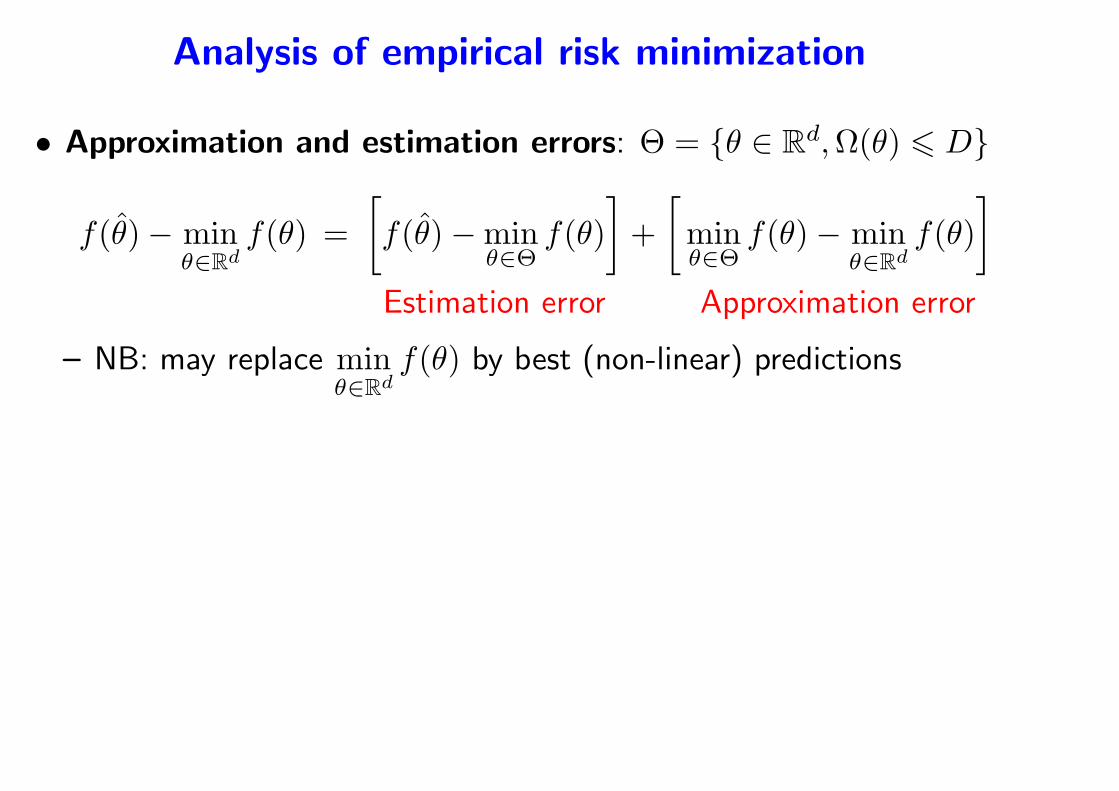
• Approximation and estimation errors: Θ = θ ∈ Rd,Ω(θ) 6 D
f(θ)− minθ∈Rd
f(θ) =
[
f(θ)−minθ∈Θ
f(θ)
]
+
[
minθ∈Θ
f(θ)− minθ∈Rd
f(θ)
]
Estimation error Approximation error
– NB: may replace minθ∈Rd
f(θ) by best (non-linear) predictions
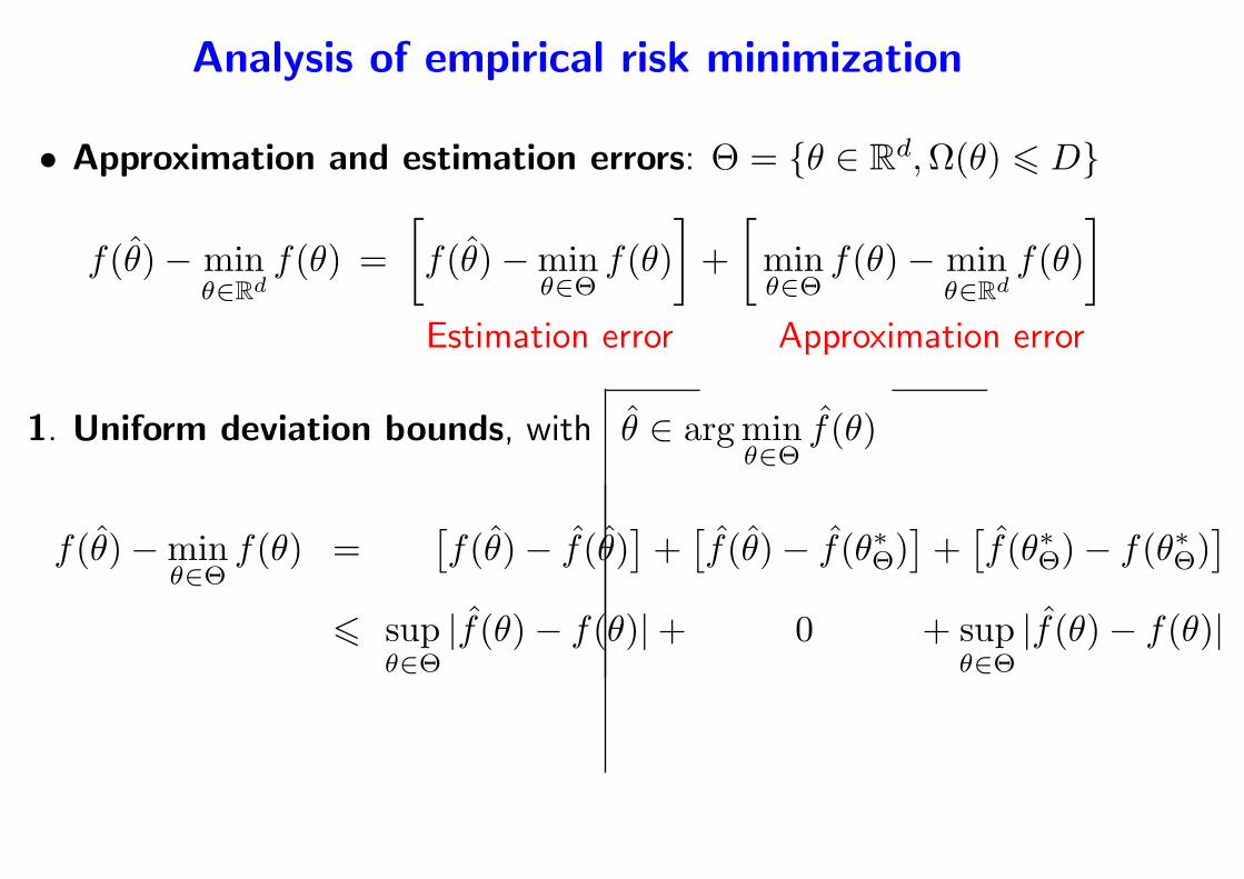
Analysis of empirical risk minimization
• Approximation and estimation errors: Θ = θ ∈ Rd,Ω(θ) 6 D
f(θ)− minθ∈Rd
f(θ) =
[
f(θ)−minθ∈Θ
f(θ)
]
+
[
minθ∈Θ
f(θ)− minθ∈Rd
f(θ)
]
Estimation error Approximation error
1. Uniform deviation bounds, with θ ∈ argminθ∈Θ
f(θ)
f(θ)−minθ∈Θ
f(θ) =[
f(θ)− f(θ)]
+[
f(θ)− f(θ∗Θ)]
+[
f(θ∗Θ)− f(θ∗Θ)]
6 supθ∈Θ
|f(θ)− f(θ)|+ 0 + supθ∈Θ
|f(θ)− f(θ)|
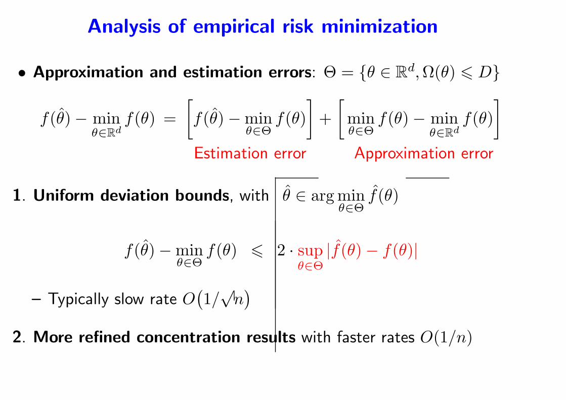
Analysis of empirical risk minimization
• Approximation and estimation errors: Θ = θ ∈ Rd,Ω(θ) 6 D
f(θ)− minθ∈Rd
f(θ) =
[
f(θ)−minθ∈Θ
f(θ)
]
+
[
minθ∈Θ
f(θ)− minθ∈Rd
f(θ)
]
Estimation error Approximation error
1. Uniform deviation bounds, with θ ∈ argminθ∈Θ
f(θ)
f(θ)−minθ∈Θ
f(θ) 6 2 · supθ∈Θ
|f(θ)− f(θ)|
– Typically slow rate O(
1/√n)
2. More refined concentration results with faster rates O(1/n)
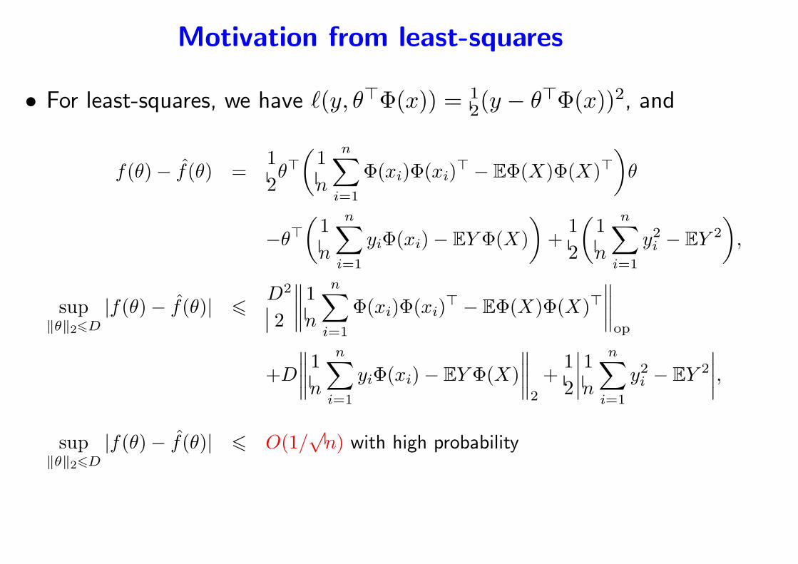
Motivation from least-squares
• For least-squares, we have ℓ(y, θ⊤Φ(x)) = 12(y − θ⊤Φ(x))2, and
f(θ)− f(θ) =1
2θ⊤
(
1
n
n∑
i=1
Φ(xi)Φ(xi)⊤ − EΦ(X)Φ(X)⊤
)
θ
−θ⊤(
1
n
n∑
i=1
yiΦ(xi)− EY Φ(X)
)
+1
2
(
1
n
n∑
i=1
y2i − EY 2
)
,
sup‖θ‖26D
|f(θ)− f(θ)| 6D2
2
∥
∥
∥
∥
1
n
n∑
i=1
Φ(xi)Φ(xi)⊤ − EΦ(X)Φ(X)⊤
∥
∥
∥
∥
op
+D
∥
∥
∥
∥
1
n
n∑
i=1
yiΦ(xi)− EY Φ(X)
∥
∥
∥
∥
2
+1
2
∣
∣
∣
∣
1
n
n∑
i=1
y2i − EY 2
∣
∣
∣
∣
,
sup‖θ‖26D
|f(θ)− f(θ)| 6 O(1/√n) with high probability
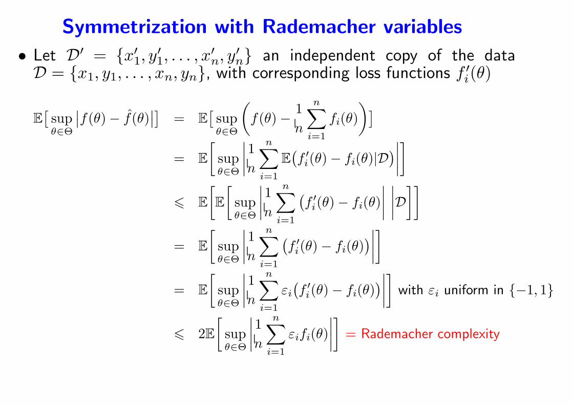
Symmetrization with Rademacher variables
• Let D′ = x′1, y
′1, . . . , x
′n, y
′n an independent copy of the data
D = x1, y1, . . . , xn, yn, with corresponding loss functions f ′i(θ)
E[
supθ∈Θ
∣
∣f(θ)− f(θ)∣
∣
]
= E[
supθ∈Θ
(
f(θ)− 1
n
n∑
i=1
fi(θ)
)
]
= E
[
supθ∈Θ
∣
∣
∣
∣
1
n
n∑
i=1
E(
f ′i(θ)− fi(θ)|D
)
∣
∣
∣
∣
]
6 E
[
E
[
supθ∈Θ
∣
∣
∣
∣
1
n
n∑
i=1
(
f ′i(θ)− fi(θ)
∣
∣
∣
∣
∣
∣
∣
∣
D]]
= E
[
supθ∈Θ
∣
∣
∣
∣
1
n
n∑
i=1
(
f ′i(θ)− fi(θ)
)
∣
∣
∣
∣
]
= E
[
supθ∈Θ
∣
∣
∣
∣
1
n
n∑
i=1
εi(
f ′i(θ)− fi(θ)
)
∣
∣
∣
∣
]
with εi uniform in −1, 1
6 2E
[
supθ∈Θ
∣
∣
∣
∣
1
n
n∑
i=1
εifi(θ)
∣
∣
∣
∣
]
= Rademacher complexity
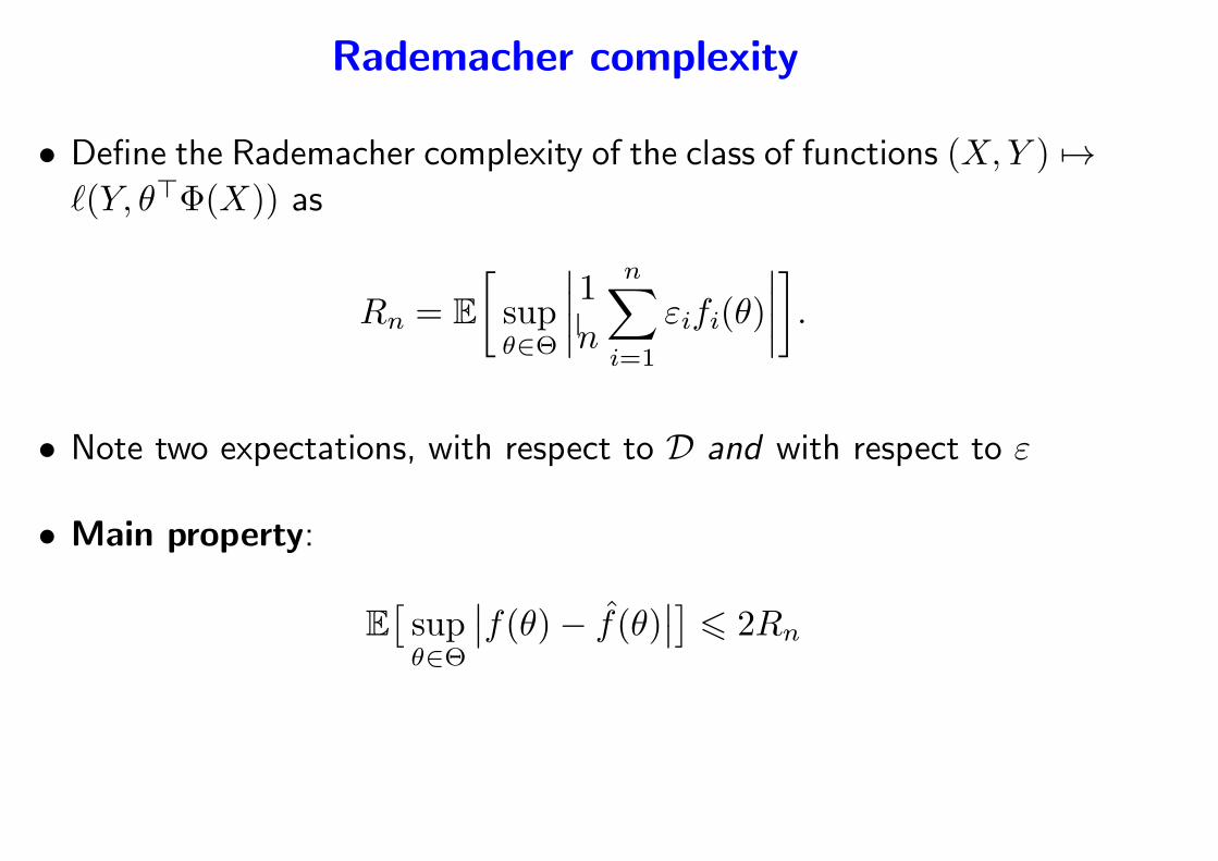
Rademacher complexity
• Define the Rademacher complexity of the class of functions (X,Y ) 7→ℓ(Y, θ⊤Φ(X)) as
Rn = E
[
supθ∈Θ
∣
∣
∣
∣
1
n
n∑
i=1
εifi(θ)
∣
∣
∣
∣
]
.
• Note two expectations, with respect to D and with respect to ε
• Main property:
E[
supθ∈Θ
∣
∣f(θ)− f(θ)∣
∣
]
6 2Rn
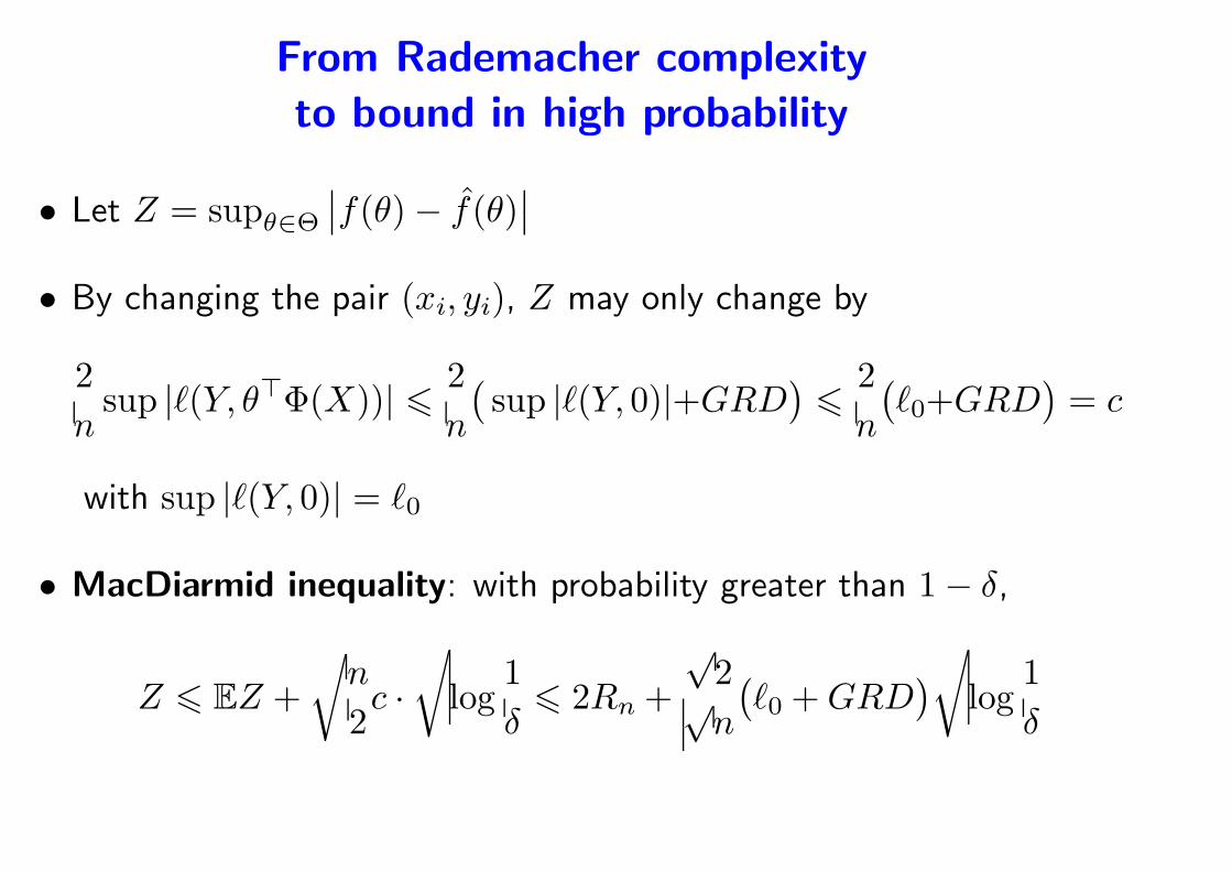
From Rademacher complexity
to bound in high probability
• Let Z = supθ∈Θ
∣
∣f(θ)− f(θ)∣
∣
• By changing the pair (xi, yi), Z may only change by
2
nsup |ℓ(Y, θ⊤Φ(X))| 6 2
n
(
sup |ℓ(Y, 0)|+GRD)
62
n
(
ℓ0+GRD)
= c
with sup |ℓ(Y, 0)| = ℓ0
• MacDiarmid inequality: with probability greater than 1− δ,
Z 6 EZ +
√
n
2c ·
√
log1
δ6 2Rn +
√2√n
(
ℓ0 +GRD)
√
log1
δ
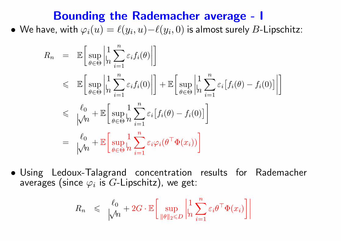
Bounding the Rademacher average - I• We have, with ϕi(u) = ℓ(yi, u)−ℓ(yi, 0) is almost surelyB-Lipschitz:
Rn = E
[
supθ∈Θ
∣
∣
∣
∣
1
n
n∑
i=1
εifi(θ)
∣
∣
∣
∣
]
6 E
[
supθ∈Θ
∣
∣
∣
∣
1
n
n∑
i=1
εifi(0)
∣
∣
∣
∣
]
+ E
[
supθ∈Θ
∣
∣
∣
∣
1
n
n∑
i=1
εi[
fi(θ)− fi(0)]
∣
∣
∣
∣
]
6ℓ0√n+ E
[
supθ∈Θ
1
n
n∑
i=1
εi[
fi(θ)− fi(0)]
]
=ℓ0√n+ E
[
supθ∈Θ
1
n
n∑
i=1
εiϕi(θ⊤Φ(xi))
]
• Using Ledoux-Talagrand concentration results for Rademacheraverages (since ϕi is G-Lipschitz), we get:
Rn 6ℓ0√n+ 2G · E
[
sup‖θ‖26D
∣
∣
∣
∣
1
n
n∑
i=1
εiθ⊤Φ(xi)
]∣
∣
∣
∣
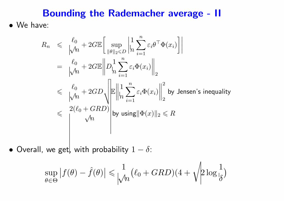
Bounding the Rademacher average - II• We have:
Rn 6ℓ0√n+ 2GE
[
sup‖θ‖26D
∣
∣
∣
∣
1
n
n∑
i=1
εiθ⊤Φ(xi)
]∣
∣
∣
∣
=ℓ0√n+ 2GE
∥
∥
∥
∥
D1
n
n∑
i=1
εiΦ(xi)
∥
∥
∥
∥
2
6ℓ0√n+ 2GD
√
√
√
√E
∥
∥
∥
∥
1
n
n∑
i=1
εiΦ(xi)
∥
∥
∥
∥
2
2
by Jensen’s inequality
62(ℓ0 +GRD)√
nby using‖Φ(x)‖2 6 R
• Overall, we get, with probability 1− δ:
supθ∈Θ
∣
∣f(θ)− f(θ)∣
∣ 61√n
(
ℓ0 +GRD)(4 +
√
2 log1
δ
)
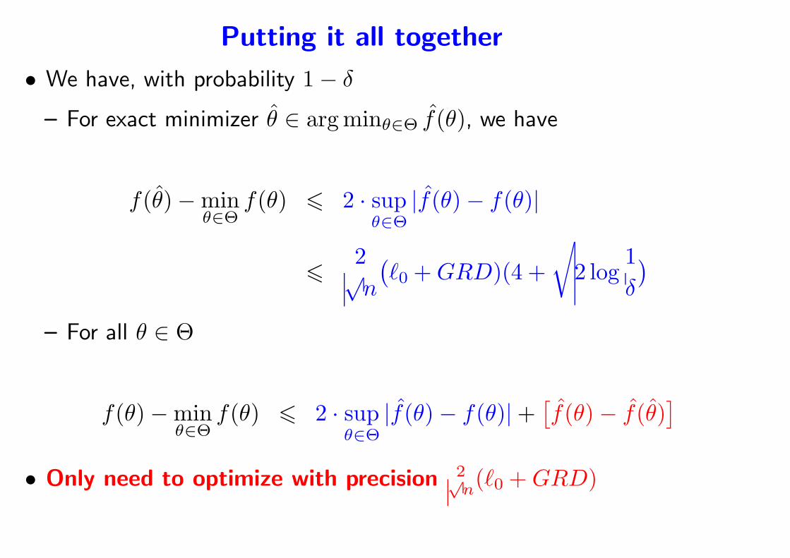
Putting it all together
• We have, with probability 1− δ
– For exact minimizer θ ∈ argminθ∈Θ f(θ), we have
f(θ)−minθ∈Θ
f(θ) 6 2 · supθ∈Θ
|f(θ)− f(θ)|
62√n
(
ℓ0 +GRD)(4 +
√
2 log1
δ
)
– For all θ ∈ Θ
f(θ)−minθ∈Θ
f(θ) 6 2 · supθ∈Θ
|f(θ)− f(θ)|+[
f(θ)− f(θ)]
• Only need to optimize with precision 2√n(ℓ0 +GRD)
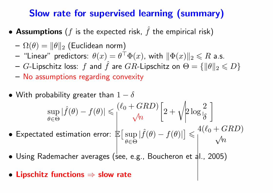
Slow rate for supervised learning (summary)
• Assumptions (f is the expected risk, f the empirical risk)
– Ω(θ) = ‖θ‖2 (Euclidean norm)
– “Linear” predictors: θ(x) = θ⊤Φ(x), with ‖Φ(x)‖2 6 R a.s.
– G-Lipschitz loss: f and f are GR-Lipschitz on Θ = ‖θ‖2 6 D– No assumptions regarding convexity
• With probability greater than 1− δ
supθ∈Θ
|f(θ)− f(θ)| 6 (ℓ0 +GRD)√n
[
2 +
√
2 log2
δ
]
• Expectated estimation error: E[
supθ∈Θ
|f(θ)− f(θ)|]
64(ℓ0 +GRD)√
n
• Using Rademacher averages (see, e.g., Boucheron et al., 2005)
• Lipschitz functions ⇒ slow rate
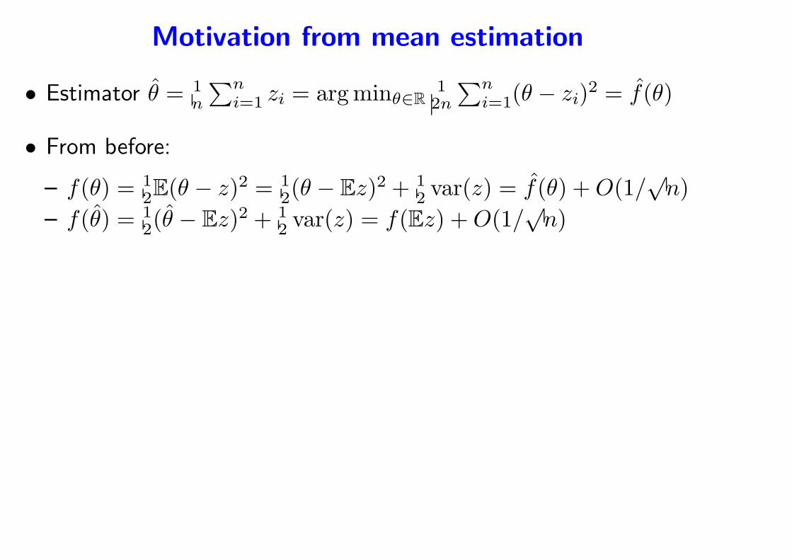
Motivation from mean estimation
• Estimator θ = 1n
∑ni=1 zi = argminθ∈R
12n
∑ni=1(θ − zi)
2 = f(θ)
• From before:
– f(θ) = 12E(θ − z)2 = 1
2(θ − Ez)2 + 12 var(z) = f(θ) +O(1/
√n)
– f(θ) = 12(θ − Ez)2 + 1
2 var(z) = f(Ez) +O(1/√n)
Motivation from mean estimation
• Estimator θ = 1n
∑ni=1 zi = argminθ∈R
12n
∑ni=1(θ − zi)
2 = f(θ)
• From before:
– f(θ) = 12E(θ − z)2 = 1
2(θ − Ez)2 + 12 var(z) = f(θ) +O(1/
√n)
– f(θ) = 12(θ − Ez)2 + 1
2 var(z) = f(Ez) +O(1/√n)
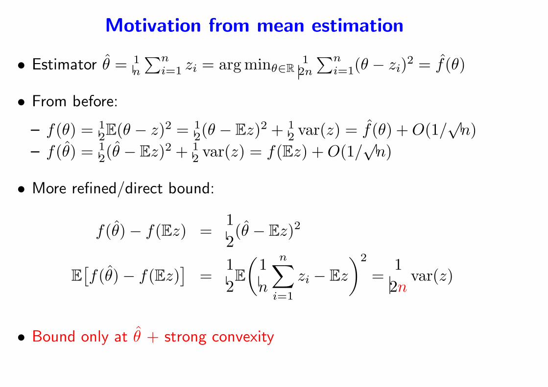
• More refined/direct bound:
f(θ)− f(Ez) =1
2(θ − Ez)2
E[
f(θ)− f(Ez)]
=1
2E
(
1
n
n∑
i=1
zi − Ez
)2
=1
2nvar(z)
• Bound only at θ + strong convexity
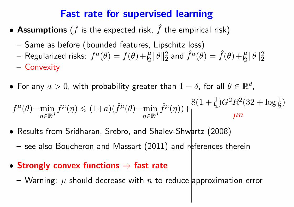
Fast rate for supervised learning
• Assumptions (f is the expected risk, f the empirical risk)
– Same as before (bounded features, Lipschitz loss)
– Regularized risks: fµ(θ) = f(θ)+µ2‖θ‖22 and fµ(θ) = f(θ)+µ
2‖θ‖22– Convexity
• For any a > 0, with probability greater than 1− δ, for all θ ∈ Rd,
fµ(θ)−minη∈Rd
fµ(η) 6 (1+a)(fµ(θ)−minη∈Rd
fµ(η))+8(1 + 1
a)G2R2(32 + log 1
δ)
µn
• Results from Sridharan, Srebro, and Shalev-Shwartz (2008)
– see also Boucheron and Massart (2011) and references therein
• Strongly convex functions ⇒ fast rate
– Warning: µ should decrease with n to reduce approximation error
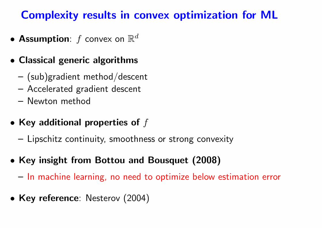
Complexity results in convex optimization for ML
• Assumption: f convex on Rd
• Classical generic algorithms
– (sub)gradient method/descent
– Accelerated gradient descent
– Newton method
• Key additional properties of f
– Lipschitz continuity, smoothness or strong convexity
• Key insight from Bottou and Bousquet (2008)
– In machine learning, no need to optimize below estimation error
• Key reference: Nesterov (2004)
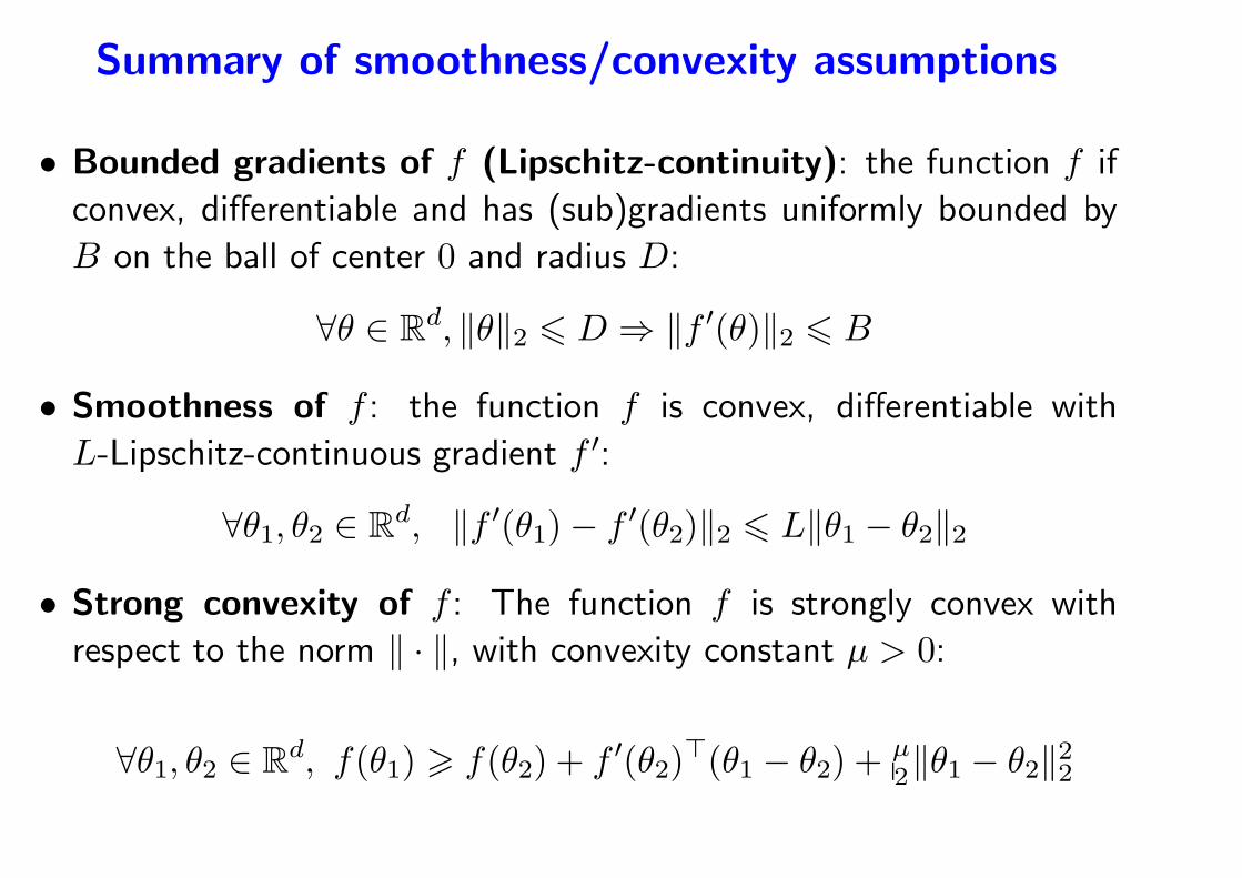
Summary of smoothness/convexity assumptions
• Bounded gradients of f (Lipschitz-continuity): the function f if
convex, differentiable and has (sub)gradients uniformly bounded by
B on the ball of center 0 and radius D:
∀θ ∈ Rd, ‖θ‖2 6 D ⇒ ‖f ′(θ)‖2 6 B
• Smoothness of f : the function f is convex, differentiable with
L-Lipschitz-continuous gradient f ′:
∀θ1, θ2 ∈ Rd, ‖f ′(θ1)− f ′(θ2)‖2 6 L‖θ1 − θ2‖2
• Strong convexity of f : The function f is strongly convex with
respect to the norm ‖ · ‖, with convexity constant µ > 0:
∀θ1, θ2 ∈ Rd, f(θ1) > f(θ2) + f ′(θ2)
⊤(θ1 − θ2) +µ2‖θ1 − θ2‖22
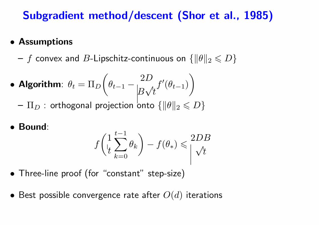
Subgradient method/descent (Shor et al., 1985)
• Assumptions
– f convex and B-Lipschitz-continuous on ‖θ‖2 6 D
• Algorithm: θt = ΠD
(
θt−1 −2D
B√tf ′(θt−1)
)
– ΠD : orthogonal projection onto ‖θ‖2 6 D
• Bound:
f
(
1
t
t−1∑
k=0
θk
)
− f(θ∗) 62DB√
t
• Three-line proof (for “constant” step-size)
• Best possible convergence rate after O(d) iterations
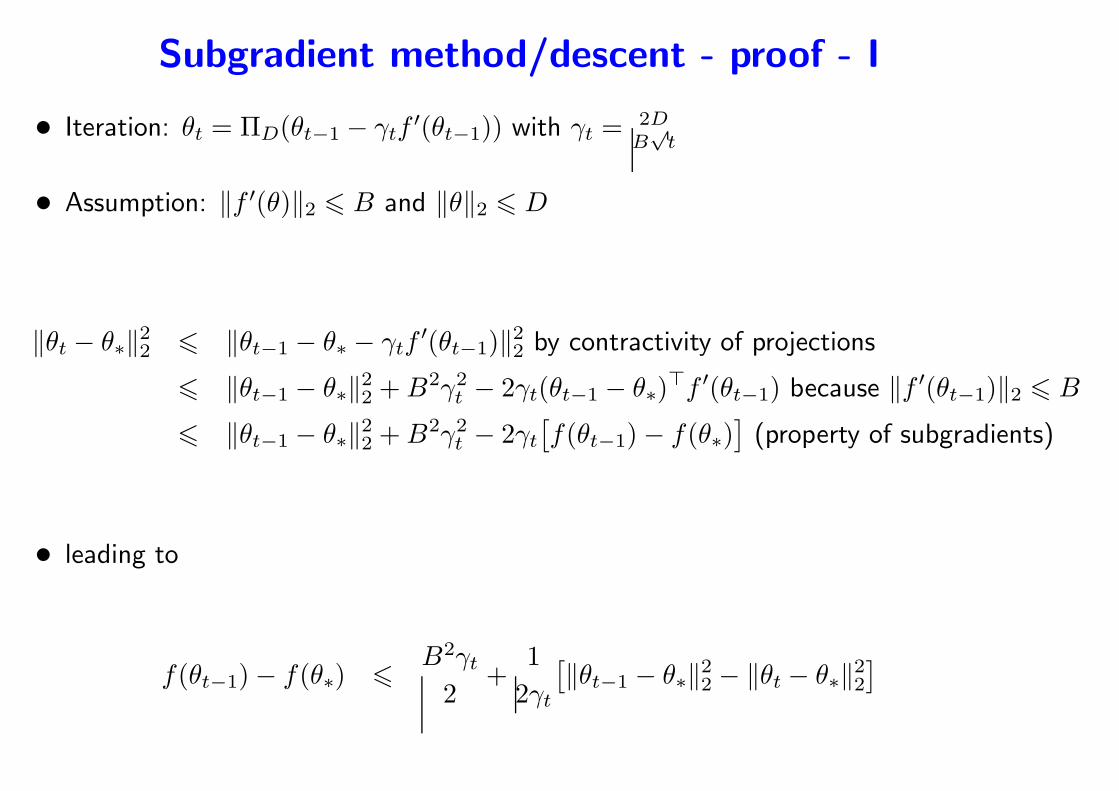
Subgradient method/descent - proof - I
• Iteration: θt = ΠD(θt−1 − γtf′(θt−1)) with γt =
2DB√t
• Assumption: ‖f ′(θ)‖2 6 B and ‖θ‖2 6 D
‖θt − θ∗‖22 6 ‖θt−1 − θ∗ − γtf′(θt−1)‖22 by contractivity of projections
6 ‖θt−1 − θ∗‖22 +B2γ2t − 2γt(θt−1 − θ∗)
⊤f ′(θt−1) because ‖f ′(θt−1)‖2 6 B
6 ‖θt−1 − θ∗‖22 +B2γ2t − 2γt
[
f(θt−1)− f(θ∗)]
(property of subgradients)
• leading to
f(θt−1)− f(θ∗) 6B2γt2
+1
2γt
[
‖θt−1 − θ∗‖22 − ‖θt − θ∗‖22]
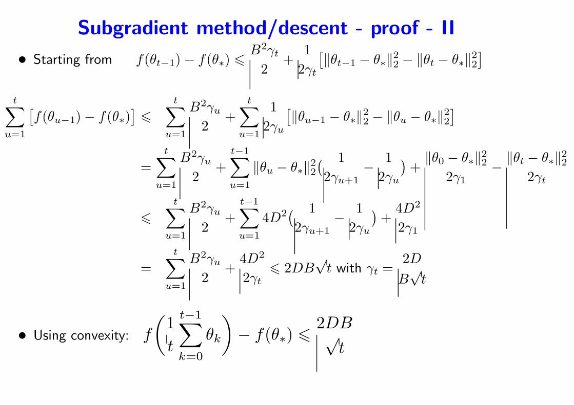
Subgradient method/descent - proof - II
• Starting from f(θt−1)− f(θ∗) 6B2γt2
+1
2γt
[
‖θt−1 − θ∗‖22 − ‖θt − θ∗‖22]
t∑
u=1
[
f(θu−1)− f(θ∗)]
6
t∑
u=1
B2γu2
+t
∑
u=1
1
2γu
[
‖θu−1 − θ∗‖22 − ‖θu − θ∗‖22]
=t
∑
u=1
B2γu2
+t−1∑
u=1
‖θu − θ∗‖22( 1
2γu+1− 1
2γu
)
+‖θ0 − θ∗‖22
2γ1− ‖θt − θ∗‖22
2γt
6
t∑
u=1
B2γu2
+t−1∑
u=1
4D2( 1
2γu+1− 1
2γu
)
+4D2
2γ1
=t
∑
u=1
B2γu2
+4D2
2γt6 2DB
√t with γt =
2D
B√t
• Using convexity: f
(
1
t
t−1∑
k=0
θk
)
− f(θ∗) 62DB√
t
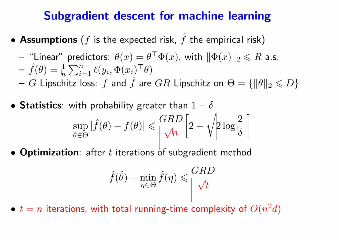
Subgradient descent for machine learning
• Assumptions (f is the expected risk, f the empirical risk)
– “Linear” predictors: θ(x) = θ⊤Φ(x), with ‖Φ(x)‖2 6 R a.s.
– f(θ) = 1n
∑ni=1 ℓ(yi,Φ(xi)
⊤θ)
– G-Lipschitz loss: f and f are GR-Lipschitz on Θ = ‖θ‖2 6 D
• Statistics: with probability greater than 1− δ
supθ∈Θ
|f(θ)− f(θ)| 6 GRD√n
[
2 +
√
2 log2
δ
]
• Optimization: after t iterations of subgradient method
f(θ)−minη∈Θ
f(η) 6GRD√
t
• t = n iterations, with total running-time complexity of O(n2d)
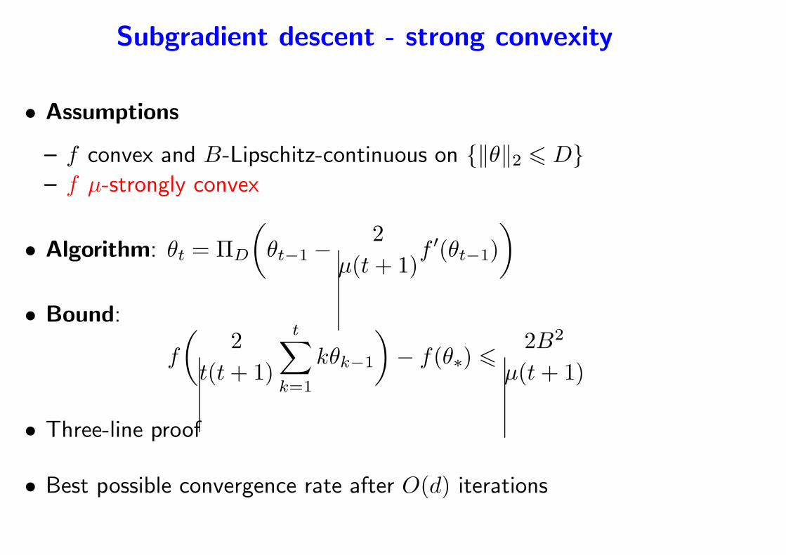
Subgradient descent - strong convexity
• Assumptions
– f convex and B-Lipschitz-continuous on ‖θ‖2 6 D– f µ-strongly convex
• Algorithm: θt = ΠD
(
θt−1 −2
µ(t+ 1)f ′(θt−1)
)
• Bound:
f
(
2
t(t+ 1)
t∑
k=1
kθk−1
)
− f(θ∗) 62B2
µ(t+ 1)
• Three-line proof
• Best possible convergence rate after O(d) iterations
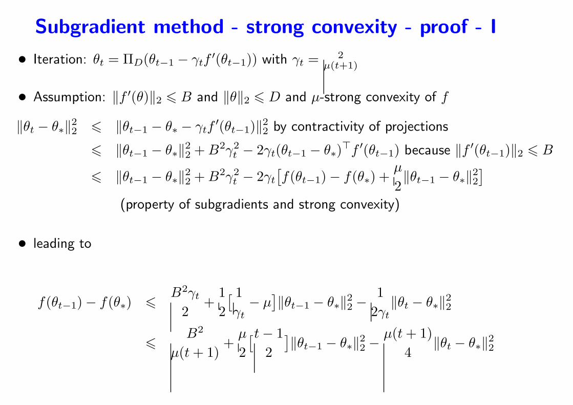
Subgradient method - strong convexity - proof - I
• Iteration: θt = ΠD(θt−1 − γtf′(θt−1)) with γt =
2µ(t+1)
• Assumption: ‖f ′(θ)‖2 6 B and ‖θ‖2 6 D and µ-strong convexity of f
‖θt − θ∗‖22 6 ‖θt−1 − θ∗ − γtf′(θt−1)‖22 by contractivity of projections
6 ‖θt−1 − θ∗‖22 +B2γ2t − 2γt(θt−1 − θ∗)
⊤f ′(θt−1) because ‖f ′(θt−1)‖2 6 B
6 ‖θt−1 − θ∗‖22 +B2γ2t − 2γt
[
f(θt−1)− f(θ∗) +µ
2‖θt−1 − θ∗‖22
]
(property of subgradients and strong convexity)
• leading to
f(θt−1)− f(θ∗) 6B2γt2
+1
2
[ 1
γt− µ
]
‖θt−1 − θ∗‖22 −1
2γt‖θt − θ∗‖22
6B2
µ(t+ 1)+
µ
2
[t− 1
2
]
‖θt−1 − θ∗‖22 −µ(t+ 1)
4‖θt − θ∗‖22
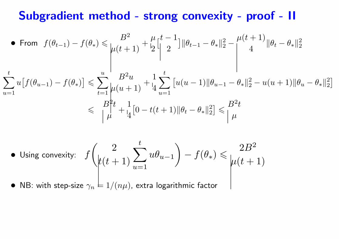
Subgradient method - strong convexity - proof - II
• From f(θt−1)− f(θ∗) 6B2
µ(t+ 1)+
µ
2
[t− 1
2
]
‖θt−1 − θ∗‖22 −µ(t+ 1)
4‖θt − θ∗‖22
t∑
u=1
u[
f(θu−1)− f(θ∗)]
6
u∑
t=1
B2u
µ(u+ 1)+
1
4
t∑
u=1
[
u(u− 1)‖θu−1 − θ∗‖22 − u(u+ 1)‖θu − θ∗‖22]
6B2t
µ+
1
4
[
0− t(t+ 1)‖θt − θ∗‖22]
6B2t
µ
• Using convexity: f
(
2
t(t+ 1)
t∑
u=1
uθu−1
)
− f(θ∗) 62B2
µ(t+ 1)
• NB: with step-size γn = 1/(nµ), extra logarithmic factor
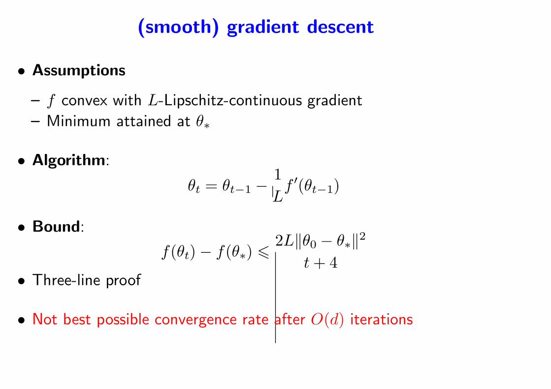
(smooth) gradient descent
• Assumptions
– f convex with L-Lipschitz-continuous gradient
– Minimum attained at θ∗
• Algorithm:
θt = θt−1 −1
Lf ′(θt−1)
• Bound:
f(θt)− f(θ∗) 62L‖θ0 − θ∗‖2
t+ 4• Three-line proof
• Not best possible convergence rate after O(d) iterations
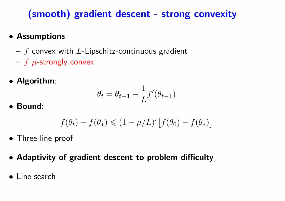
(smooth) gradient descent - strong convexity
• Assumptions
– f convex with L-Lipschitz-continuous gradient
– f µ-strongly convex
• Algorithm:
θt = θt−1 −1
Lf ′(θt−1)
• Bound:
f(θt)− f(θ∗) 6 (1− µ/L)t[
f(θ0)− f(θ∗)]
• Three-line proof
• Adaptivity of gradient descent to problem difficulty
• Line search
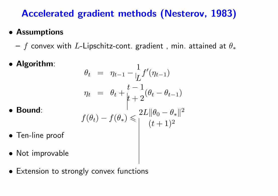
Accelerated gradient methods (Nesterov, 1983)
• Assumptions
– f convex with L-Lipschitz-cont. gradient , min. attained at θ∗
• Algorithm:θt = ηt−1 −
1
Lf ′(ηt−1)
ηt = θt +t− 1
t+ 2(θt − θt−1)
• Bound:f(θt)− f(θ∗) 6
2L‖θ0 − θ∗‖2(t+ 1)2
• Ten-line proof
• Not improvable
• Extension to strongly convex functions
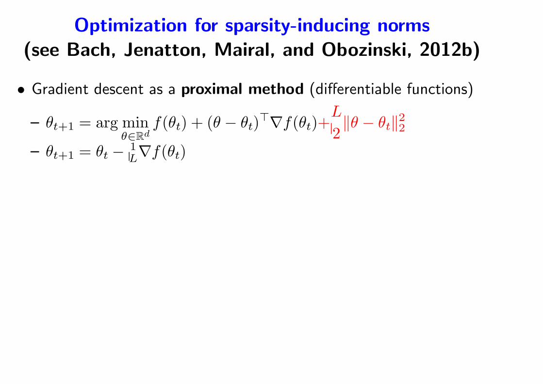
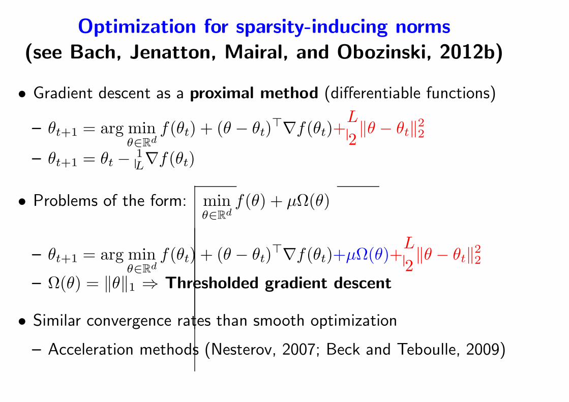
Optimization for sparsity-inducing norms
(see Bach, Jenatton, Mairal, and Obozinski, 2012b)
• Gradient descent as a proximal method (differentiable functions)
– θt+1 = arg minθ∈Rd
f(θt) + (θ − θt)⊤∇f(θt)+
L
2‖θ − θt‖22
– θt+1 = θt − 1L∇f(θt)
Optimization for sparsity-inducing norms
(see Bach, Jenatton, Mairal, and Obozinski, 2012b)
• Gradient descent as a proximal method (differentiable functions)
– θt+1 = arg minθ∈Rd
f(θt) + (θ − θt)⊤∇f(θt)+
L
2‖θ − θt‖22
– θt+1 = θt − 1L∇f(θt)
• Problems of the form: minθ∈Rd
f(θ) + µΩ(θ)
– θt+1 = arg minθ∈Rd
f(θt) + (θ − θt)⊤∇f(θt)+µΩ(θ)+
L
2‖θ − θt‖22
– Ω(θ) = ‖θ‖1 ⇒ Thresholded gradient descent
• Similar convergence rates than smooth optimization
– Acceleration methods (Nesterov, 2007; Beck and Teboulle, 2009)
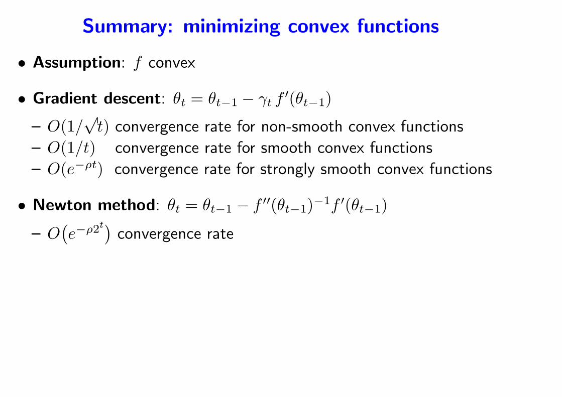
Summary: minimizing convex functions
• Assumption: f convex
• Gradient descent: θt = θt−1 − γt f′(θt−1)
– O(1/√t) convergence rate for non-smooth convex functions
– O(1/t) convergence rate for smooth convex functions
– O(e−ρt) convergence rate for strongly smooth convex functions
• Newton method: θt = θt−1 − f ′′(θt−1)−1f ′(θt−1)
– O(
e−ρ2t)
convergence rate
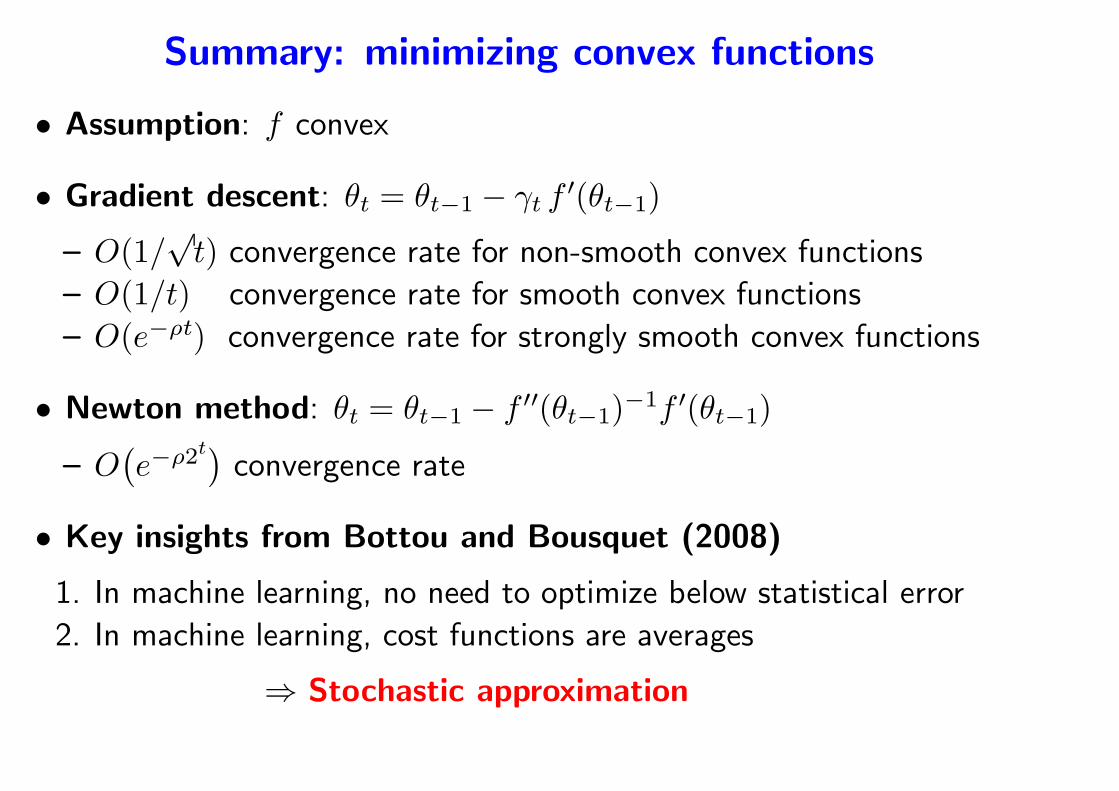
• Key insights from Bottou and Bousquet (2008)
1. In machine learning, no need to optimize below statistical error
2. In machine learning, cost functions are averages
⇒ Stochastic approximation

Outline
1. Large-scale machine learning and optimization
• Traditional statistical analysis
• Classical methods for convex optimization
2. Non-smooth stochastic approximation
• Stochastic (sub)gradient and averaging
• Non-asymptotic results and lower bounds
• Strongly convex vs. non-strongly convex
3. Smooth stochastic approximation algorithms
• Asymptotic and non-asymptotic results
• Beyond decaying step-sizes
4. Finite data sets
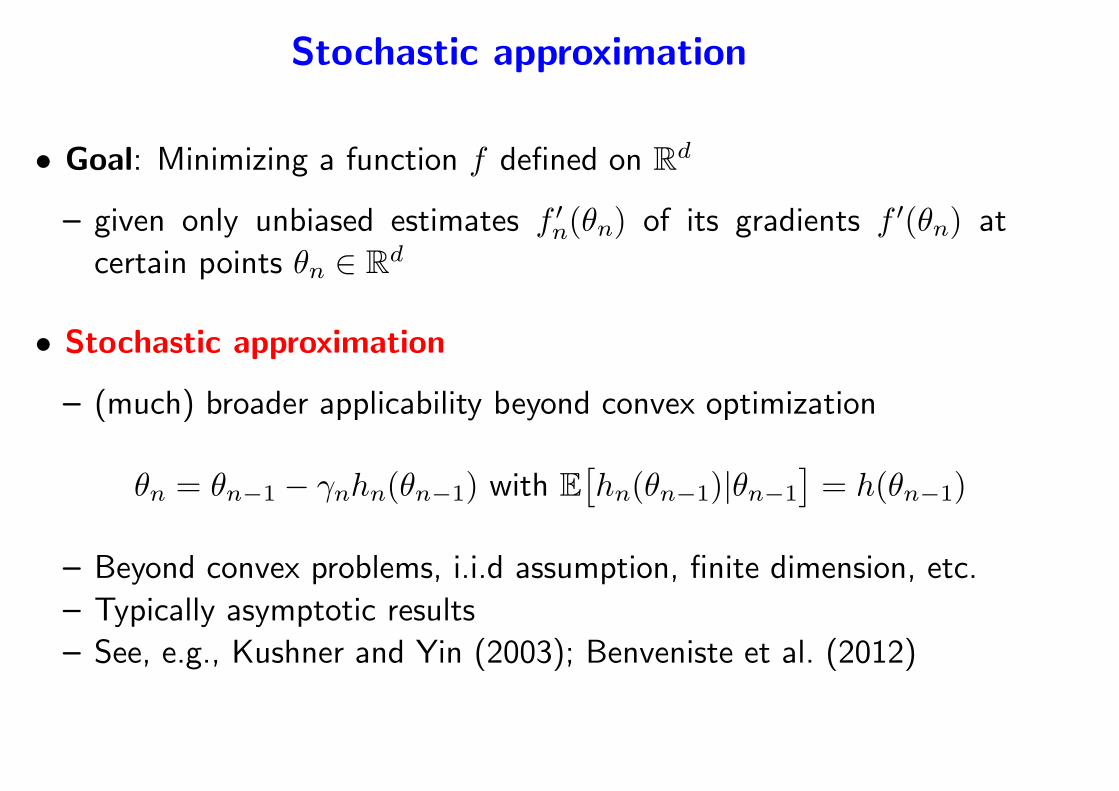
Stochastic approximation
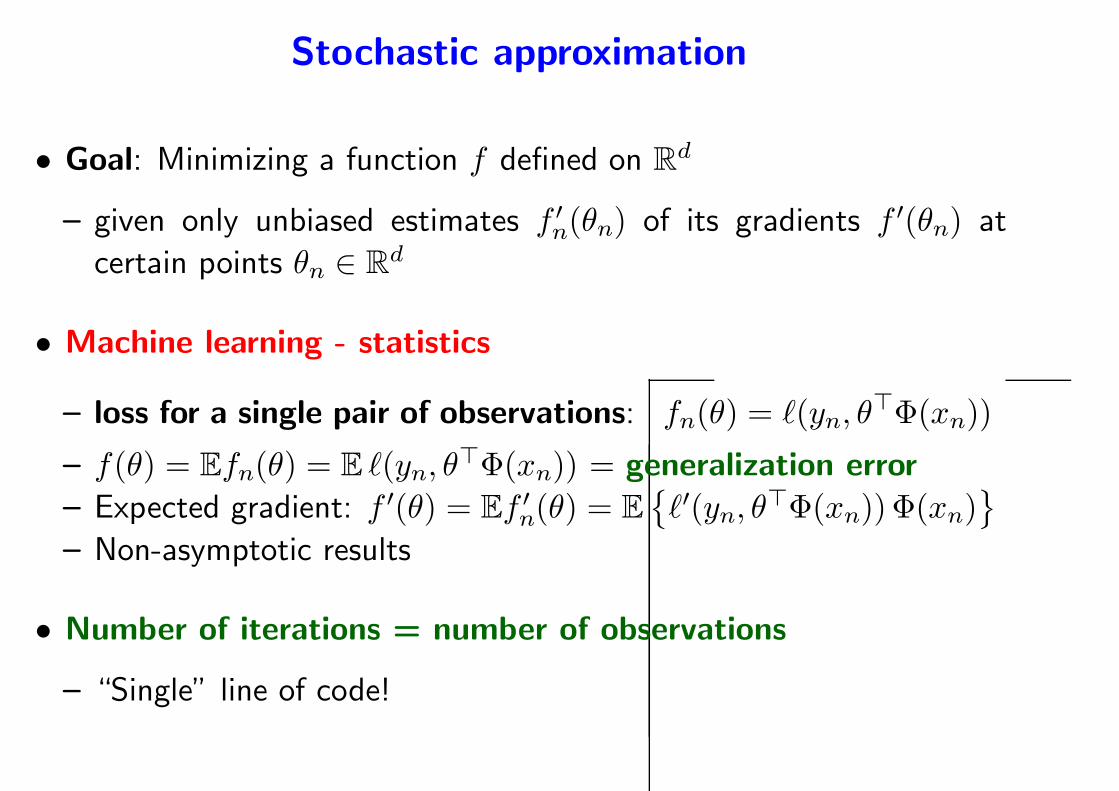
• Goal: Minimizing a function f defined on Rd
– given only unbiased estimates f ′n(θn) of its gradients f ′(θn) at
certain points θn ∈ Rd
• Stochastic approximation
– (much) broader applicability beyond convex optimization
θn = θn−1 − γnhn(θn−1) with E[
hn(θn−1)|θn−1
]
= h(θn−1)
– Beyond convex problems, i.i.d assumption, finite dimension, etc.
– Typically asymptotic results
– See, e.g., Kushner and Yin (2003); Benveniste et al. (2012)
Stochastic approximation
• Goal: Minimizing a function f defined on Rd
– given only unbiased estimates f ′n(θn) of its gradients f ′(θn) at
certain points θn ∈ Rd
• Machine learning - statistics
– loss for a single pair of observations: fn(θ) = ℓ(yn, θ⊤Φ(xn))
– f(θ) = Efn(θ) = E ℓ(yn, θ⊤Φ(xn)) = generalization error
– Expected gradient: f ′(θ) = Ef ′n(θ) = E
ℓ′(yn, θ⊤Φ(xn))Φ(xn)
– Non-asymptotic results
• Number of iterations = number of observations
– “Single” line of code!
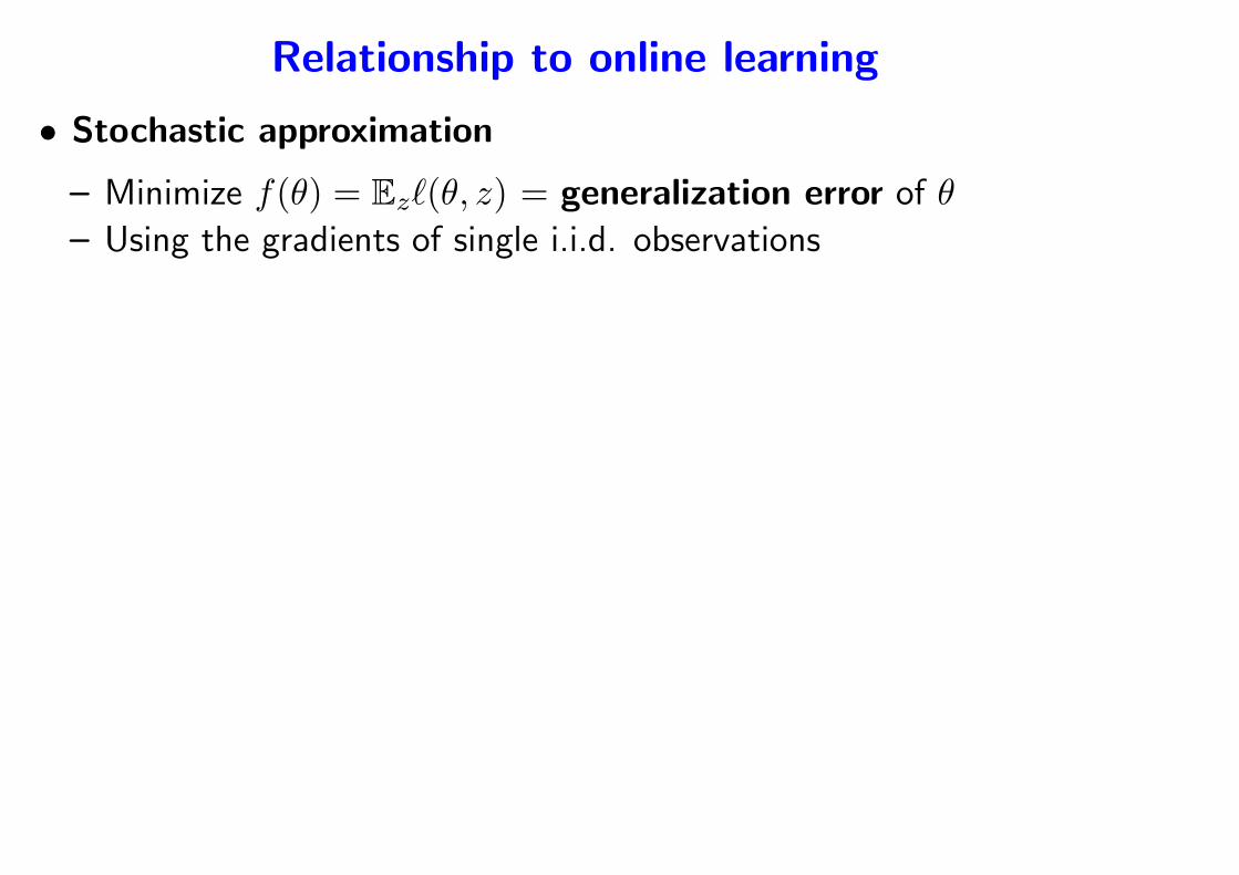
Relationship to online learning
• Stochastic approximation
– Minimize f(θ) = Ezℓ(θ, z) = generalization error of θ
– Using the gradients of single i.i.d. observations
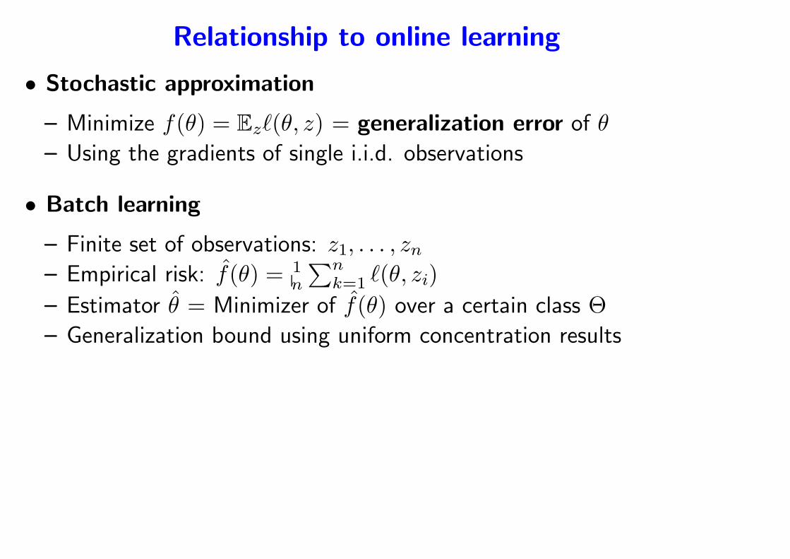
Relationship to online learning
• Stochastic approximation
– Minimize f(θ) = Ezℓ(θ, z) = generalization error of θ
– Using the gradients of single i.i.d. observations
• Batch learning
– Finite set of observations: z1, . . . , zn– Empirical risk: f(θ) = 1
n
∑nk=1 ℓ(θ, zi)
– Estimator θ = Minimizer of f(θ) over a certain class Θ
– Generalization bound using uniform concentration results
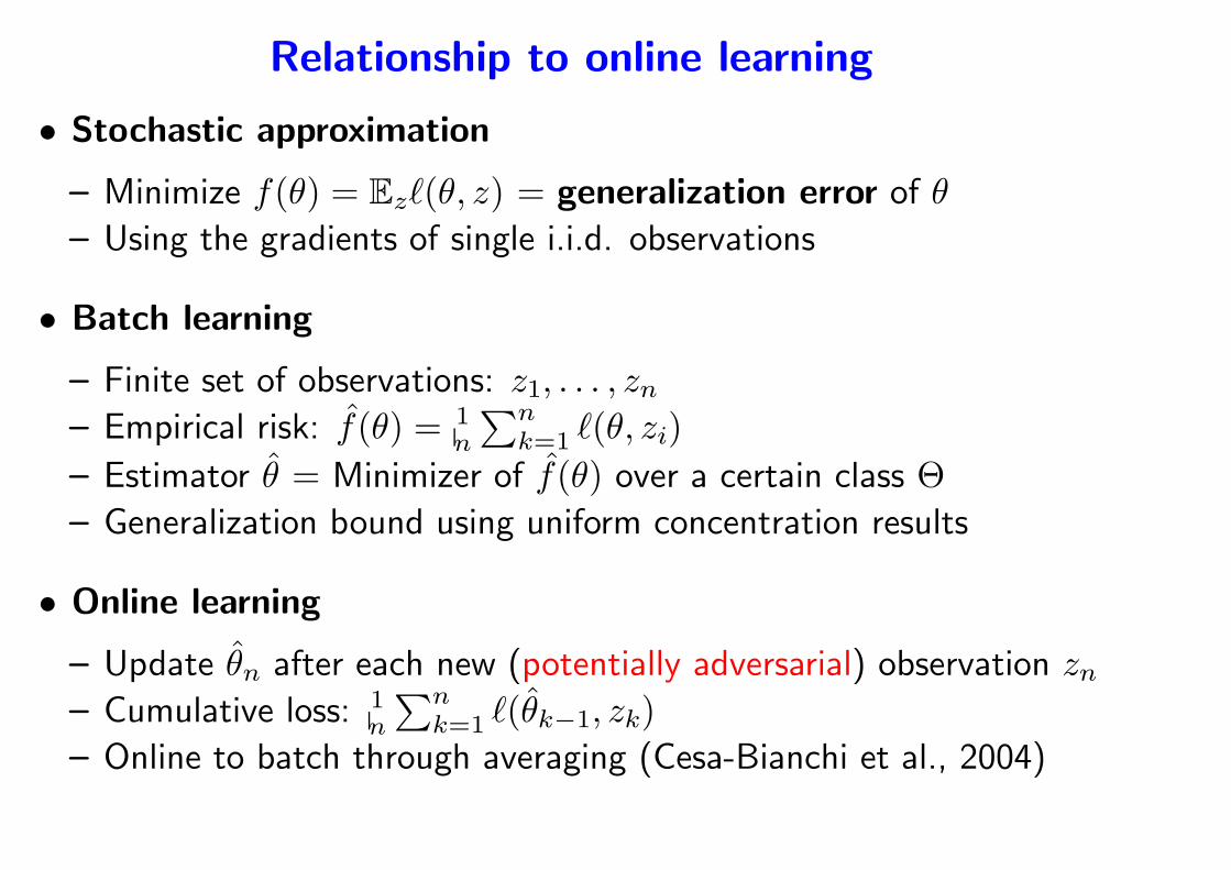
• Online learning
– Update θn after each new (potentially adversarial) observation zn– Cumulative loss: 1
n
∑nk=1 ℓ(θk−1, zk)
– Online to batch through averaging (Cesa-Bianchi et al., 2004)
Convex stochastic approximation
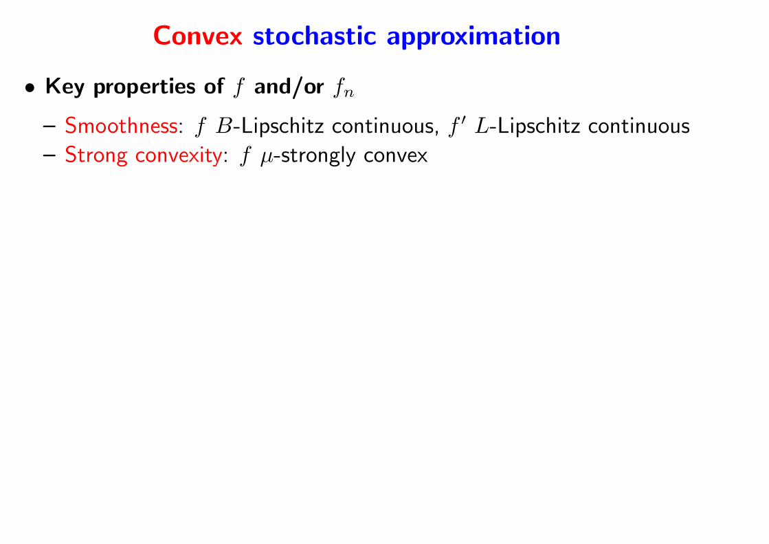
• Key properties of f and/or fn
– Smoothness: f B-Lipschitz continuous, f ′ L-Lipschitz continuous
– Strong convexity: f µ-strongly convex
Convex stochastic approximation
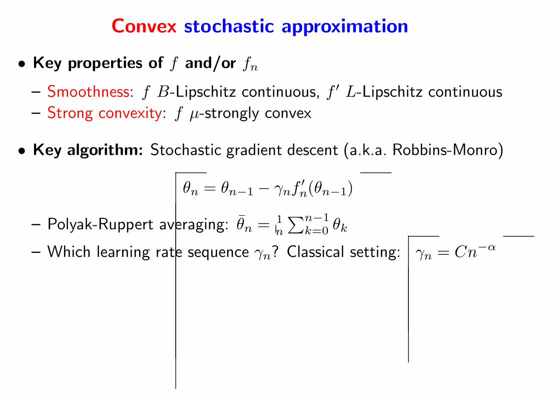
• Key properties of f and/or fn
– Smoothness: f B-Lipschitz continuous, f ′ L-Lipschitz continuous
– Strong convexity: f µ-strongly convex
• Key algorithm: Stochastic gradient descent (a.k.a. Robbins-Monro)
θn = θn−1 − γnf′n(θn−1)
– Polyak-Ruppert averaging: θn = 1n
∑n−1k=0 θk
– Which learning rate sequence γn? Classical setting: γn = Cn−α
Convex stochastic approximation
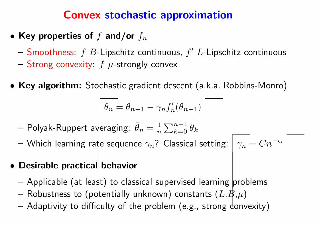
• Key properties of f and/or fn
– Smoothness: f B-Lipschitz continuous, f ′ L-Lipschitz continuous
– Strong convexity: f µ-strongly convex
• Key algorithm: Stochastic gradient descent (a.k.a. Robbins-Monro)
θn = θn−1 − γnf′n(θn−1)
– Polyak-Ruppert averaging: θn = 1n
∑n−1k=0 θk
– Which learning rate sequence γn? Classical setting: γn = Cn−α
• Desirable practical behavior
– Applicable (at least) to classical supervised learning problems
– Robustness to (potentially unknown) constants (L,B,µ)
– Adaptivity to difficulty of the problem (e.g., strong convexity)
Stochastic subgradient descent/method
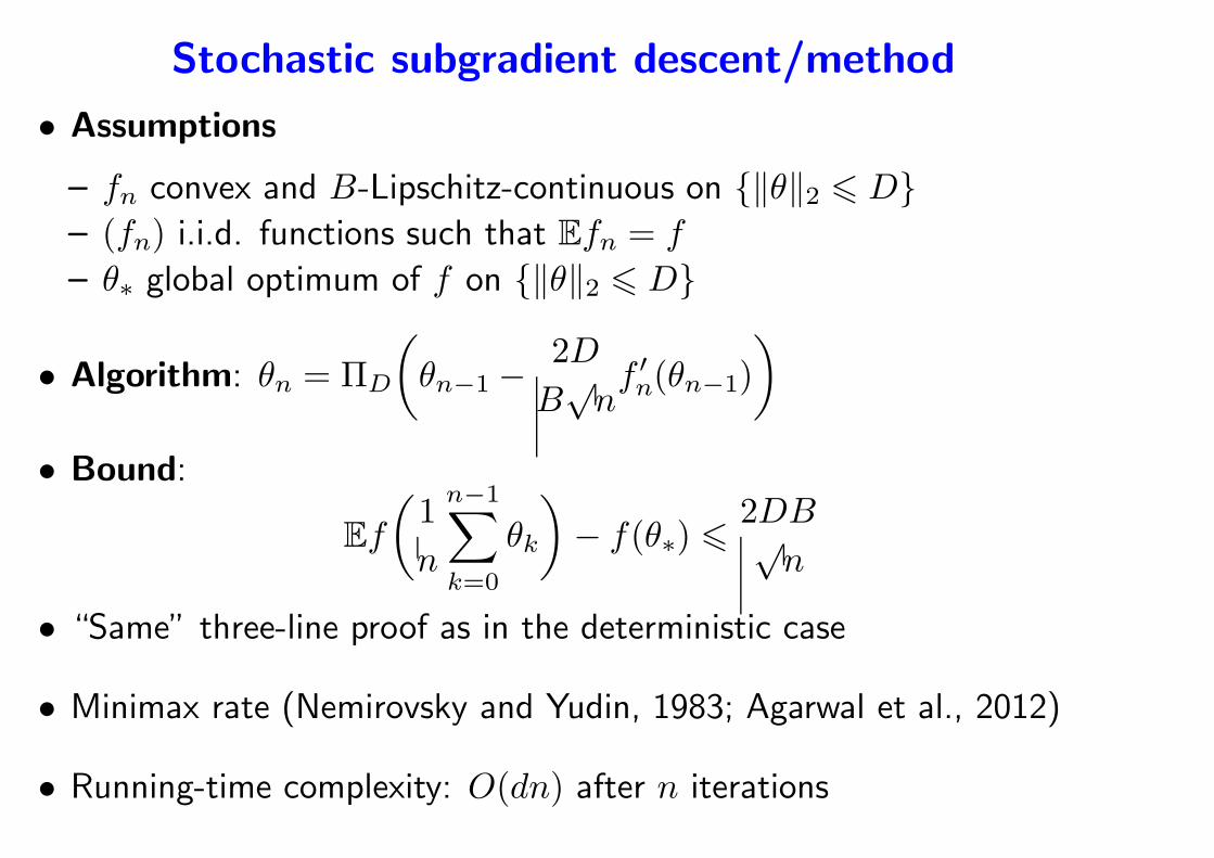
• Assumptions
– fn convex and B-Lipschitz-continuous on ‖θ‖2 6 D– (fn) i.i.d. functions such that Efn = f
– θ∗ global optimum of f on ‖θ‖2 6 D
• Algorithm: θn = ΠD
(
θn−1 −2D
B√nf ′n(θn−1)
)
• Bound:
Ef
(
1
n
n−1∑
k=0
θk
)
− f(θ∗) 62DB√
n
• “Same” three-line proof as in the deterministic case
• Minimax rate (Nemirovsky and Yudin, 1983; Agarwal et al., 2012)
• Running-time complexity: O(dn) after n iterations
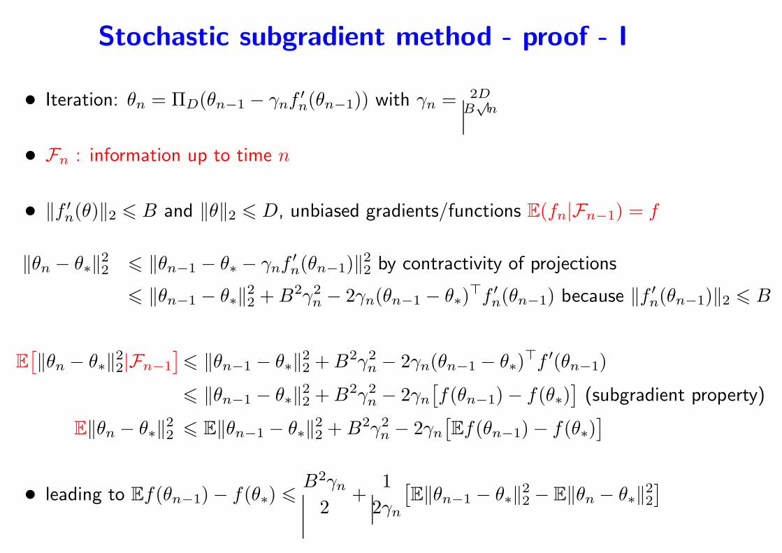
Stochastic subgradient method - proof - I
• Iteration: θn = ΠD(θn−1 − γnf′n(θn−1)) with γn = 2D
B√n
• Fn : information up to time n
• ‖f ′n(θ)‖2 6 B and ‖θ‖2 6 D, unbiased gradients/functions E(fn|Fn−1) = f
‖θn − θ∗‖22 6 ‖θn−1 − θ∗ − γnf′n(θn−1)‖22 by contractivity of projections
6 ‖θn−1 − θ∗‖22 +B2γ2n − 2γn(θn−1 − θ∗)
⊤f ′n(θn−1) because ‖f ′
n(θn−1)‖2 6 B
E[
‖θn − θ∗‖22|Fn−1
]
6 ‖θn−1 − θ∗‖22 +B2γ2n − 2γn(θn−1 − θ∗)
⊤f ′(θn−1)
6 ‖θn−1 − θ∗‖22 +B2γ2n − 2γn
[
f(θn−1)− f(θ∗)]
(subgradient property)
E‖θn − θ∗‖22 6 E‖θn−1 − θ∗‖22 + B2γ2n − 2γn
[
Ef(θn−1)− f(θ∗)]
• leading to Ef(θn−1)− f(θ∗) 6B2γn2
+1
2γn
[
E‖θn−1 − θ∗‖22 − E‖θn − θ∗‖22]
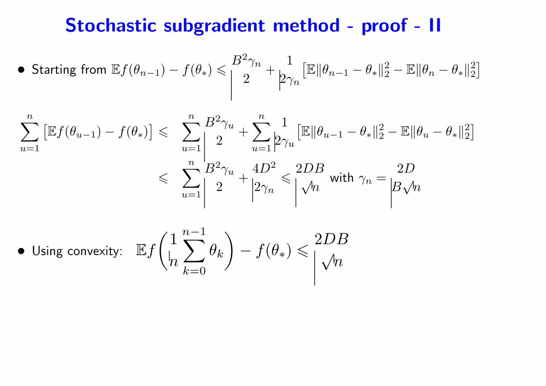
Stochastic subgradient method - proof - II
• Starting from Ef(θn−1)− f(θ∗) 6B2γn2
+1
2γn
[
E‖θn−1 − θ∗‖22 − E‖θn − θ∗‖22]
n∑
u=1
[
Ef(θu−1)− f(θ∗)]
6
n∑
u=1
B2γu2
+n∑
u=1
1
2γu
[
E‖θu−1 − θ∗‖22 − E‖θu − θ∗‖22]
6
n∑
u=1
B2γu2
+4D2
2γn6
2DB√n
with γn =2D
B√n
• Using convexity: Ef
(
1
n
n−1∑
k=0
θk
)
− f(θ∗) 62DB√
n
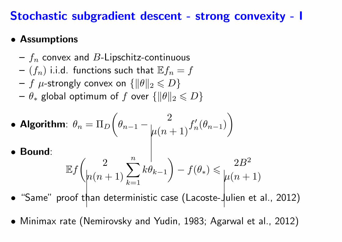
Stochastic subgradient descent - strong convexity - I
• Assumptions
– fn convex and B-Lipschitz-continuous
– (fn) i.i.d. functions such that Efn = f
– f µ-strongly convex on ‖θ‖2 6 D– θ∗ global optimum of f over ‖θ‖2 6 D
• Algorithm: θn = ΠD
(
θn−1 −2
µ(n+ 1)f ′n(θn−1)
)
• Bound:
Ef
(
2
n(n+ 1)
n∑
k=1
kθk−1
)
− f(θ∗) 62B2
µ(n+ 1)
• “Same” proof than deterministic case (Lacoste-Julien et al., 2012)
• Minimax rate (Nemirovsky and Yudin, 1983; Agarwal et al., 2012)
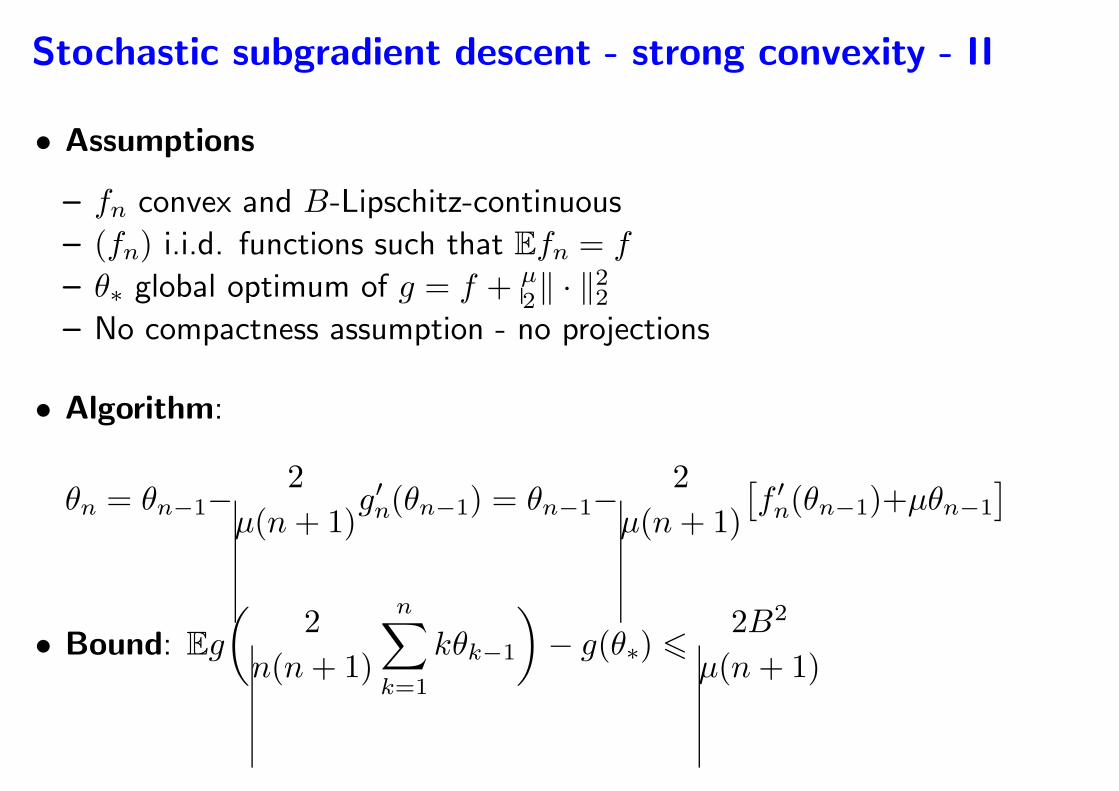
Stochastic subgradient descent - strong convexity - II
• Assumptions
– fn convex and B-Lipschitz-continuous
– (fn) i.i.d. functions such that Efn = f
– θ∗ global optimum of g = f + µ2‖ · ‖22
– No compactness assumption - no projections
• Algorithm:
θn = θn−1−2
µ(n+ 1)g′n(θn−1) = θn−1−
2
µ(n+ 1)
[
f ′n(θn−1)+µθn−1
]
• Bound: Eg
(
2
n(n+ 1)
n∑
k=1
kθk−1
)
− g(θ∗) 62B2
µ(n+ 1)

Outline
1. Large-scale machine learning and optimization
• Traditional statistical analysis
• Classical methods for convex optimization
2. Non-smooth stochastic approximation
• Stochastic (sub)gradient and averaging
• Non-asymptotic results and lower bounds
• Strongly convex vs. non-strongly convex
3. Smooth stochastic approximation algorithms
• Asymptotic and non-asymptotic results
• Beyond decaying step-sizes
4. Finite data sets
Convex stochastic approximation
Existing work
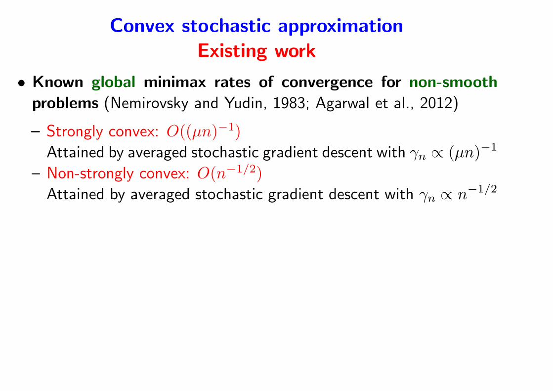
• Known global minimax rates of convergence for non-smooth
problems (Nemirovsky and Yudin, 1983; Agarwal et al., 2012)
– Strongly convex: O((µn)−1)
Attained by averaged stochastic gradient descent with γn ∝ (µn)−1
– Non-strongly convex: O(n−1/2)
Attained by averaged stochastic gradient descent with γn ∝ n−1/2
– Bottou and Le Cun (2005); Bottou and Bousquet (2008); Hazan
et al. (2007); Shalev-Shwartz and Srebro (2008); Shalev-Shwartz
et al. (2007, 2009); Xiao (2010); Duchi and Singer (2009); Nesterov
and Vial (2008); Nemirovski et al. (2009)
Convex stochastic approximation
Existing work
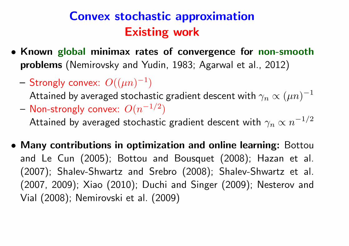
• Known global minimax rates of convergence for non-smooth
problems (Nemirovsky and Yudin, 1983; Agarwal et al., 2012)
– Strongly convex: O((µn)−1)
Attained by averaged stochastic gradient descent with γn ∝ (µn)−1
– Non-strongly convex: O(n−1/2)
Attained by averaged stochastic gradient descent with γn ∝ n−1/2
• Many contributions in optimization and online learning: Bottou
and Le Cun (2005); Bottou and Bousquet (2008); Hazan et al.
(2007); Shalev-Shwartz and Srebro (2008); Shalev-Shwartz et al.
(2007, 2009); Xiao (2010); Duchi and Singer (2009); Nesterov and
Vial (2008); Nemirovski et al. (2009)
Convex stochastic approximation
Existing work
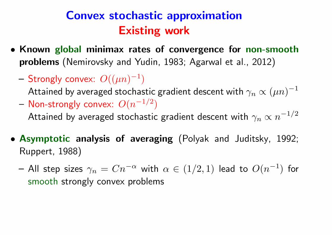
• Known global minimax rates of convergence for non-smooth
problems (Nemirovsky and Yudin, 1983; Agarwal et al., 2012)
– Strongly convex: O((µn)−1)
Attained by averaged stochastic gradient descent with γn ∝ (µn)−1
– Non-strongly convex: O(n−1/2)
Attained by averaged stochastic gradient descent with γn ∝ n−1/2
• Asymptotic analysis of averaging (Polyak and Juditsky, 1992;
Ruppert, 1988)
– All step sizes γn = Cn−α with α ∈ (1/2, 1) lead to O(n−1) for
smooth strongly convex problems
A single algorithm with global adaptive convergence rate for
smooth problems?
Convex stochastic approximation
Existing work
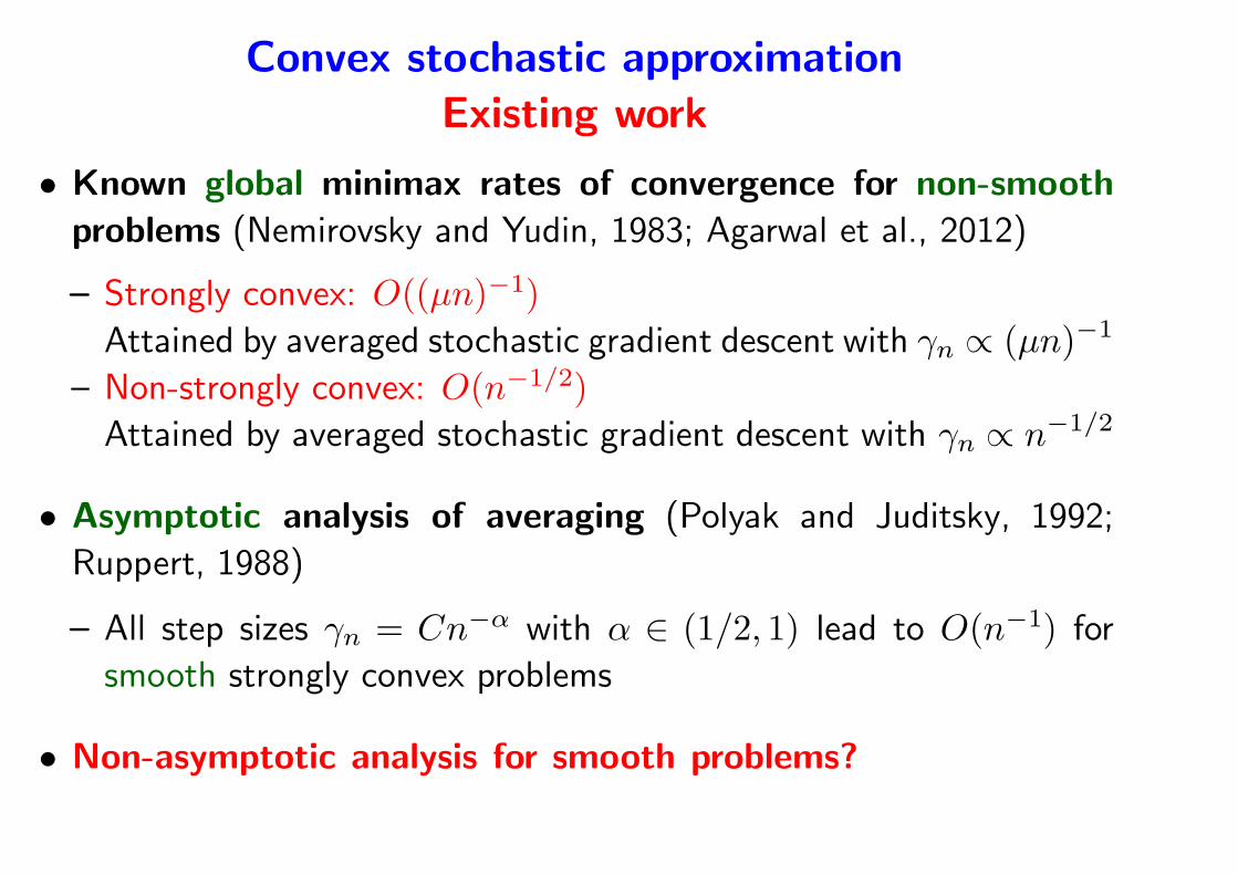
• Known global minimax rates of convergence for non-smooth
problems (Nemirovsky and Yudin, 1983; Agarwal et al., 2012)
– Strongly convex: O((µn)−1)
Attained by averaged stochastic gradient descent with γn ∝ (µn)−1
– Non-strongly convex: O(n−1/2)
Attained by averaged stochastic gradient descent with γn ∝ n−1/2
• Asymptotic analysis of averaging (Polyak and Juditsky, 1992;
Ruppert, 1988)
– All step sizes γn = Cn−α with α ∈ (1/2, 1) lead to O(n−1) for
smooth strongly convex problems
• Non-asymptotic analysis for smooth problems? problems with
convergence rate O(min1/µn, 1/√n)
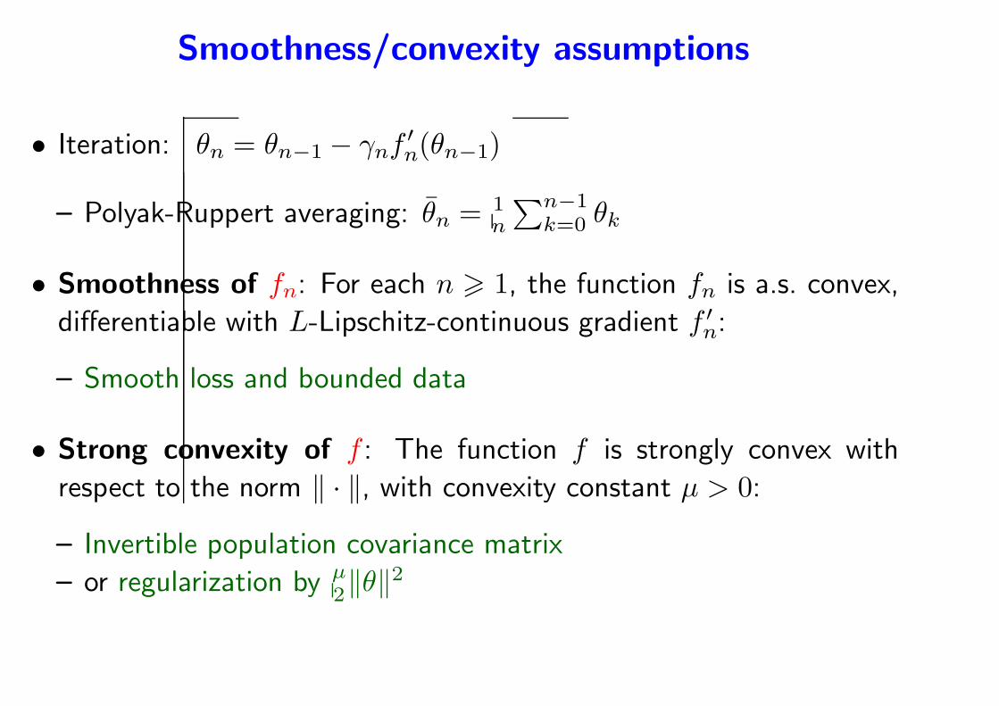
Smoothness/convexity assumptions
• Iteration: θn = θn−1 − γnf′n(θn−1)
– Polyak-Ruppert averaging: θn = 1n
∑n−1k=0 θk
• Smoothness of fn: For each n > 1, the function fn is a.s. convex,
differentiable with L-Lipschitz-continuous gradient f ′n:
– Smooth loss and bounded data
• Strong convexity of f : The function f is strongly convex with
respect to the norm ‖ · ‖, with convexity constant µ > 0:
– Invertible population covariance matrix
– or regularization by µ2‖θ‖2
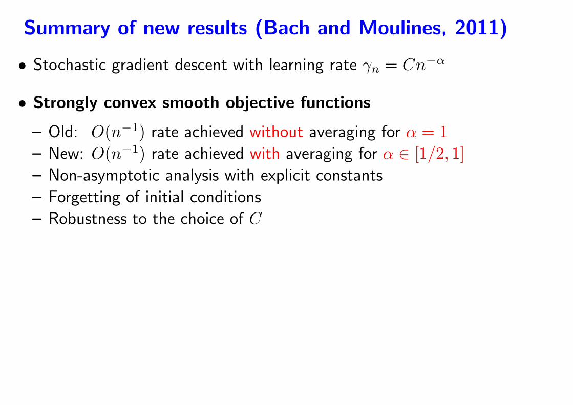
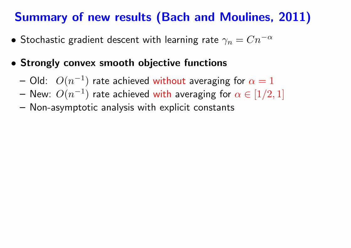
Summary of new results (Bach and Moulines, 2011)
• Stochastic gradient descent with learning rate γn = Cn−α
• Strongly convex smooth objective functions
– Old: O(n−1) rate achieved without averaging for α = 1
– New: O(n−1) rate achieved with averaging for α ∈ [1/2, 1]
– Non-asymptotic analysis with explicit constants
– Forgetting of initial conditions
– Robustness to the choice of C
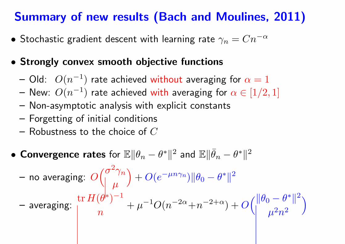
• Convergence rates for E‖θn − θ∗‖2 and E‖θn − θ∗‖2
– no averaging: O(σ2γn
µ
)
+O(e−µnγn)‖θ0 − θ∗‖2
– averaging:trH(θ∗)−1
n+ µ−1O(n−2α+n−2+α) +O
(‖θ0 − θ∗‖2µ2n2
)
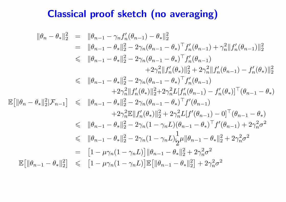
Classical proof sketch (no averaging)
‖θn − θ∗‖22 = ‖θn−1 − γnf′n(θn−1)− θ∗‖22
= ‖θn−1 − θ∗‖22 − 2γn(θn−1 − θ∗)⊤f ′
n(θn−1) + γ2n‖f ′
n(θn−1)‖226 ‖θn−1 − θ∗‖22 − 2γn(θn−1 − θ∗)
⊤f ′n(θn−1)
+2γ2n‖f ′
n(θ∗)‖22 + 2γ2n‖f ′
n(θn−1)− f ′n(θ∗)‖22
6 ‖θn−1 − θ∗‖22 − 2γn(θn−1 − θ∗)⊤f ′
n(θn−1)
+2γ2n‖f ′
n(θ∗)‖22+2γ2nL[f
′n(θn−1)− f ′
n(θ∗)]⊤(θn−1 − θ∗)
E[
‖θn − θ∗‖22|Fn−1
]
6 ‖θn−1 − θ∗‖22 − 2γn(θn−1 − θ∗)⊤f ′(θn−1)
+2γ2nE‖f ′
n(θ∗)‖22 + 2γ2nL[f
′(θn−1)− 0]⊤(θn−1 − θ∗)
6 ‖θn−1 − θ∗‖22 − 2γn(1− γnL)(θn−1 − θ∗)⊤f ′(θn−1) + 2γ2
nσ2
6 ‖θn−1 − θ∗‖22 − 2γn(1− γnL)1
2µ‖θn−1 − θ∗‖22 + 2γ2
nσ2
=[
1− µγn(1− γnL)]
‖θn−1 − θ∗‖22 + 2γ2nσ
2
E[
‖θn−1 − θ∗‖22]
6[
1− µγn(1− γnL)]
E[
‖θn−1 − θ∗‖22]
+ 2γ2nσ
2
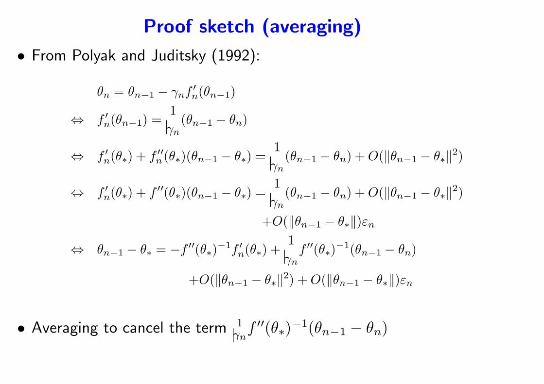
Proof sketch (averaging)
• From Polyak and Juditsky (1992):
θn = θn−1 − γnf′n(θn−1)
⇔ f ′n(θn−1) =
1
γn(θn−1 − θn)
⇔ f ′n(θ∗) + f ′′
n(θ∗)(θn−1 − θ∗) =1
γn(θn−1 − θn) +O(‖θn−1 − θ∗‖2)
⇔ f ′n(θ∗) + f ′′(θ∗)(θn−1 − θ∗) =
1
γn(θn−1 − θn) +O(‖θn−1 − θ∗‖2)
+O(‖θn−1 − θ∗‖)εn
⇔ θn−1 − θ∗ = −f ′′(θ∗)−1f ′
n(θ∗) +1
γnf ′′(θ∗)
−1(θn−1 − θn)
+O(‖θn−1 − θ∗‖2) +O(‖θn−1 − θ∗‖)εn
• Averaging to cancel the term 1γnf ′′(θ∗)−1(θn−1 − θn)
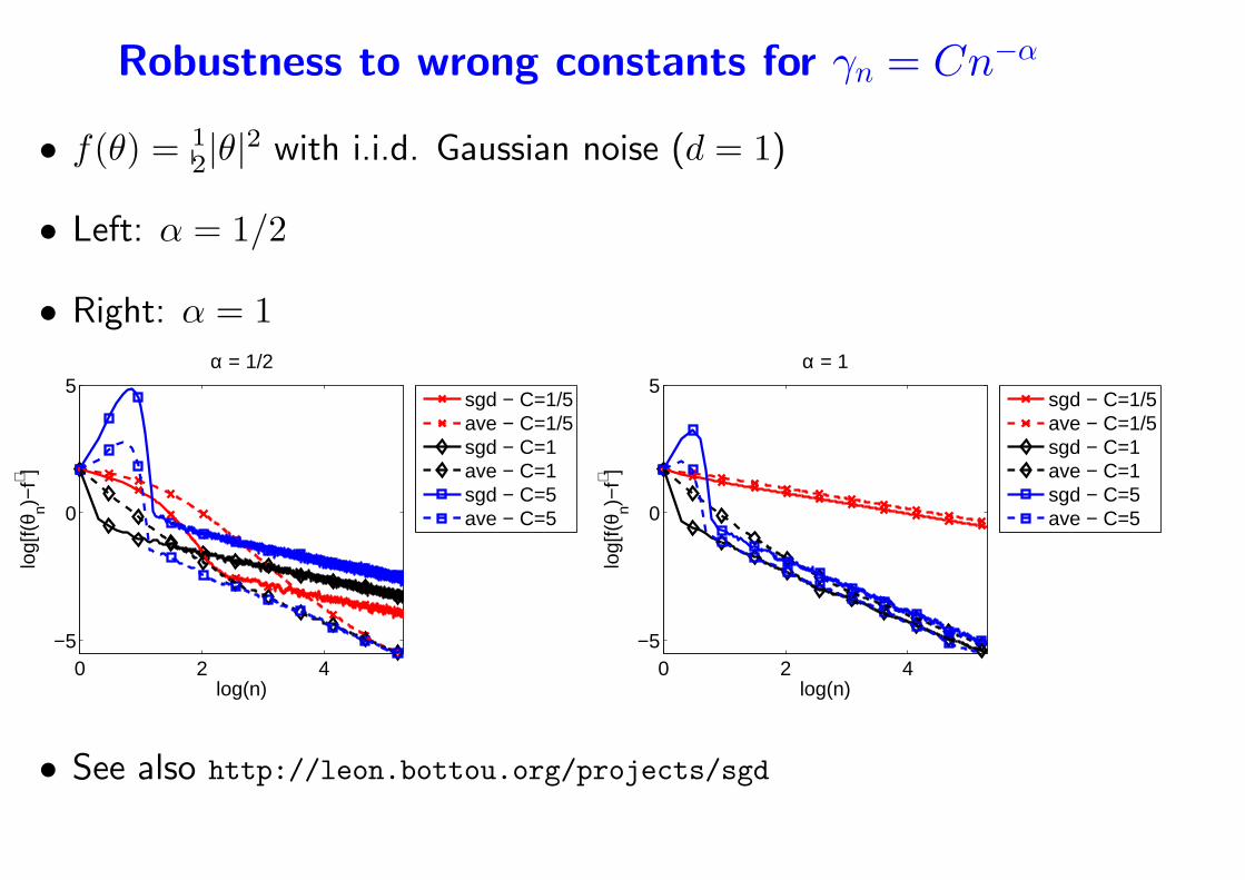
Robustness to wrong constants for γn = Cn−α
• f(θ) = 12|θ|2 with i.i.d. Gaussian noise (d = 1)
• Left: α = 1/2
• Right: α = 1
0 2 4−5
0
5
log(n)
log[
f(θ n)−
f∗ ]
α = 1/2
sgd − C=1/5ave − C=1/5sgd − C=1ave − C=1sgd − C=5ave − C=5
0 2 4−5
0
5
log(n)
log[
f(θ n)−
f∗ ]
α = 1
sgd − C=1/5ave − C=1/5sgd − C=1ave − C=1sgd − C=5ave − C=5
• See also http://leon.bottou.org/projects/sgd
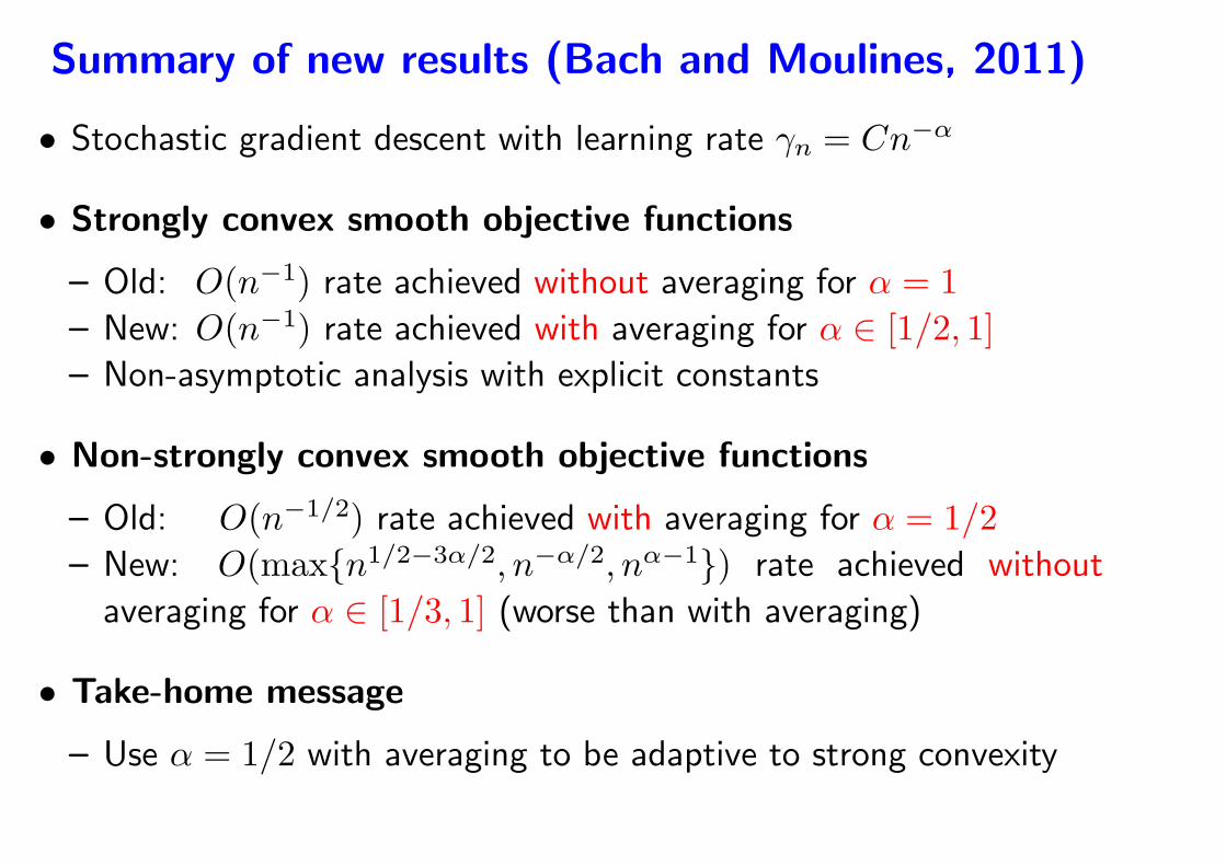
Summary of new results (Bach and Moulines, 2011)
• Stochastic gradient descent with learning rate γn = Cn−α
• Strongly convex smooth objective functions
– Old: O(n−1) rate achieved without averaging for α = 1
– New: O(n−1) rate achieved with averaging for α ∈ [1/2, 1]
– Non-asymptotic analysis with explicit constants
• Non-strongly convex smooth objective functions
– Old: O(n−1/2) rate achieved with averaging for α = 1/2
– New: O(maxn1/2−3α/2, n−α/2, nα−1) rate achieved without
averaging for α ∈ [1/3, 1] (worse than with averaging)
• Take-home message
– Use α = 1/2 with averaging to be adaptive to strong convexity
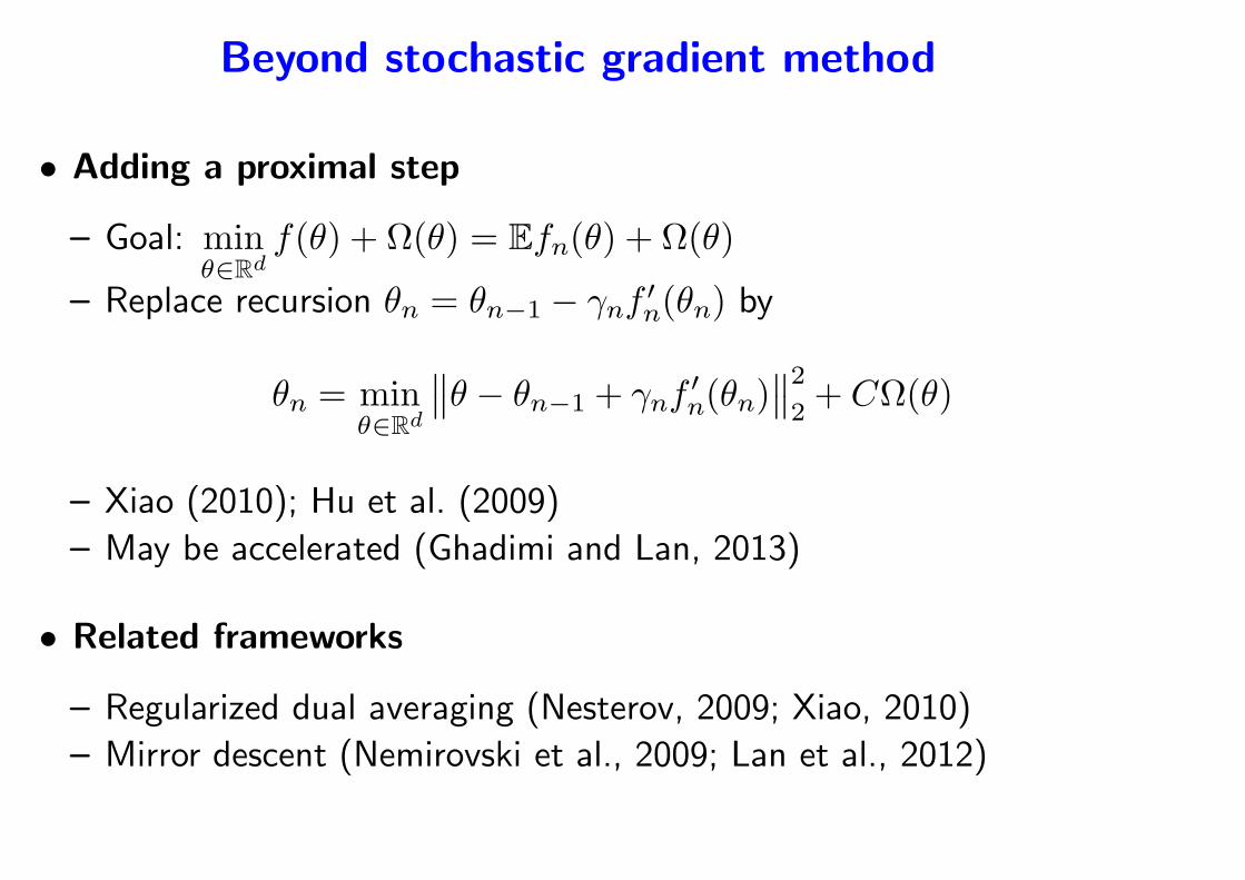
Beyond stochastic gradient method
• Adding a proximal step
– Goal: minθ∈Rd
f(θ) + Ω(θ) = Efn(θ) + Ω(θ)
– Replace recursion θn = θn−1 − γnf′n(θn) by
θn = minθ∈Rd
∥
∥θ − θn−1 + γnf′n(θn)
∥
∥
2
2+ CΩ(θ)
– Xiao (2010); Hu et al. (2009)
– May be accelerated (Ghadimi and Lan, 2013)
• Related frameworks
– Regularized dual averaging (Nesterov, 2009; Xiao, 2010)
– Mirror descent (Nemirovski et al., 2009; Lan et al., 2012)

Outline
1. Large-scale machine learning and optimization
• Traditional statistical analysis
• Classical methods for convex optimization
2. Non-smooth stochastic approximation
• Stochastic (sub)gradient and averaging
• Non-asymptotic results and lower bounds
• Strongly convex vs. non-strongly convex
3. Smooth stochastic approximation algorithms
• Asymptotic and non-asymptotic results
• Beyond decaying step-sizes
4. Finite data sets
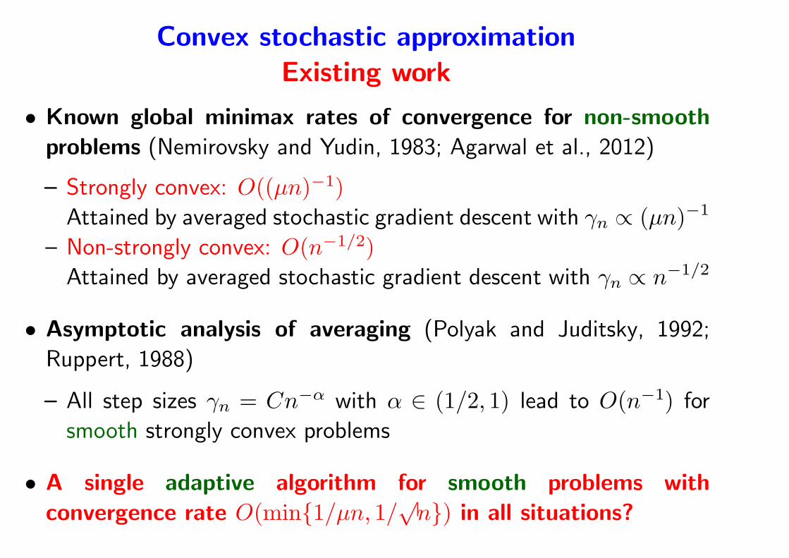
Convex stochastic approximation
Existing work
• Known global minimax rates of convergence for non-smooth
problems (Nemirovsky and Yudin, 1983; Agarwal et al., 2012)
– Strongly convex: O((µn)−1)
Attained by averaged stochastic gradient descent with γn ∝ (µn)−1
– Non-strongly convex: O(n−1/2)
Attained by averaged stochastic gradient descent with γn ∝ n−1/2
• Asymptotic analysis of averaging (Polyak and Juditsky, 1992;
Ruppert, 1988)
– All step sizes γn = Cn−α with α ∈ (1/2, 1) lead to O(n−1) for
smooth strongly convex problems
• A single adaptive algorithm for smooth problems with
convergence rate O(min1/µn, 1/√n) in all situations?
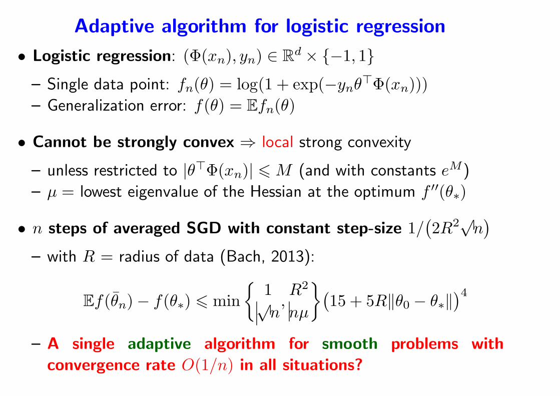
Adaptive algorithm for logistic regression
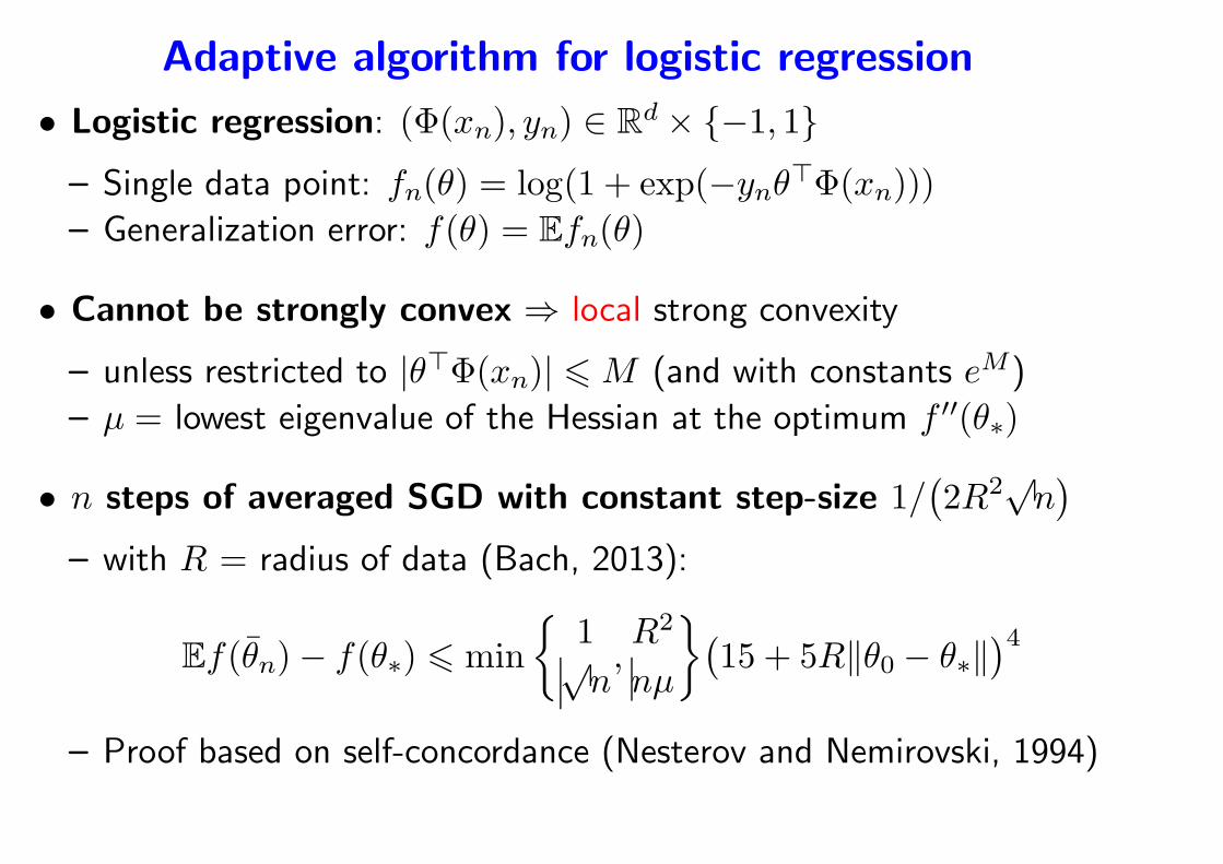
• Logistic regression: (Φ(xn), yn) ∈ Rd × −1, 1
– Single data point: fn(θ) = log(1 + exp(−ynθ⊤Φ(xn)))
– Generalization error: f(θ) = Efn(θ)
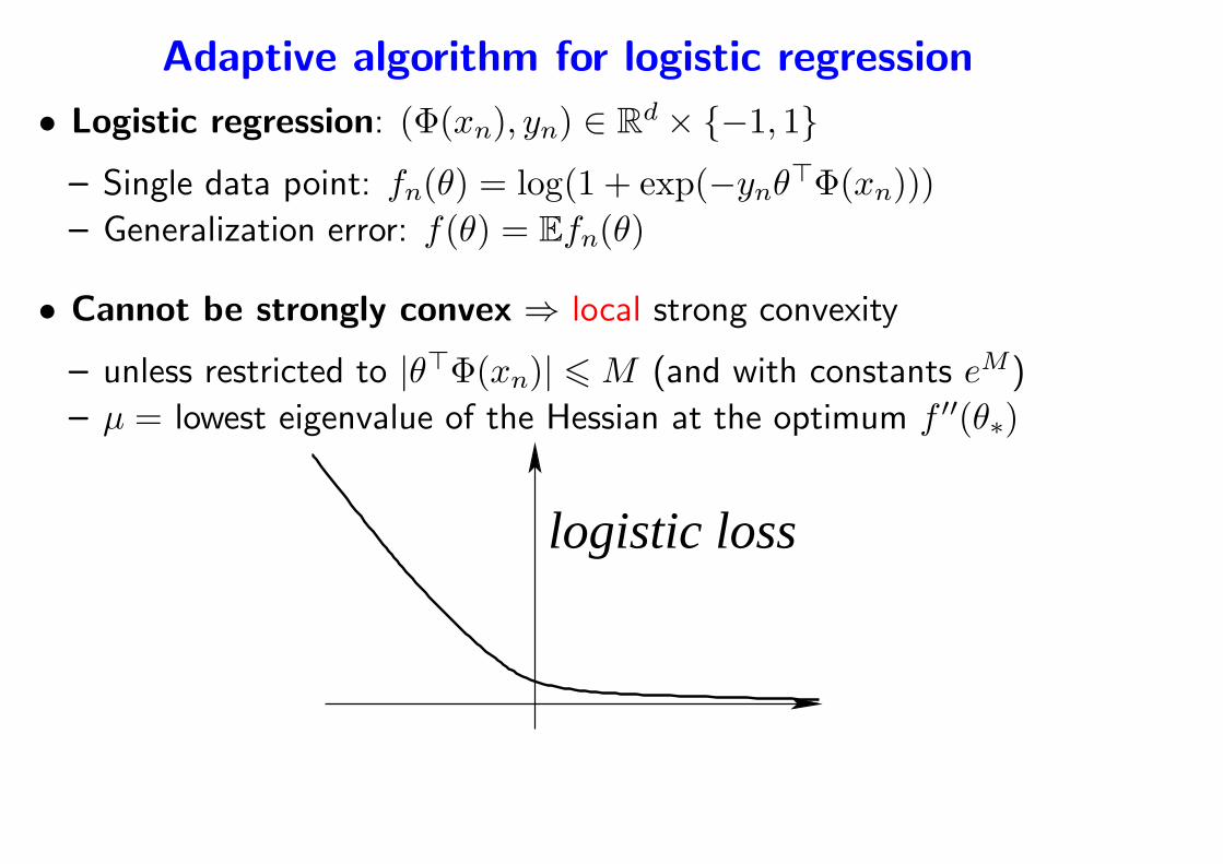
Adaptive algorithm for logistic regression
• Logistic regression: (Φ(xn), yn) ∈ Rd × −1, 1
– Single data point: fn(θ) = log(1 + exp(−ynθ⊤Φ(xn)))
– Generalization error: f(θ) = Efn(θ)
• Cannot be strongly convex ⇒ local strong convexity
– unless restricted to |θ⊤Φ(xn)| 6 M (and with constants eM)
– µ = lowest eigenvalue of the Hessian at the optimum f ′′(θ∗)
logistic loss

Adaptive algorithm for logistic regression
• Logistic regression: (Φ(xn), yn) ∈ Rd × −1, 1
– Single data point: fn(θ) = log(1 + exp(−ynθ⊤Φ(xn)))
– Generalization error: f(θ) = Efn(θ)
• Cannot be strongly convex ⇒ local strong convexity
– unless restricted to |θ⊤Φ(xn)| 6 M (and with constants eM)
– µ = lowest eigenvalue of the Hessian at the optimum f ′′(θ∗)
• n steps of averaged SGD with constant step-size 1/(
2R2√n)
– with R = radius of data (Bach, 2013):
Ef(θn)− f(θ∗) 6 min
1√n,R2
nµ
(
15 + 5R‖θ0 − θ∗‖)4
– Proof based on self-concordance (Nesterov and Nemirovski, 1994)
Self-concordance
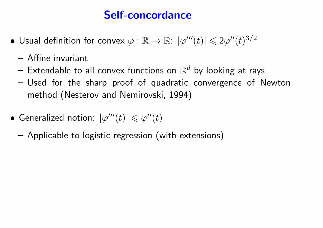
• Usual definition for convex ϕ : R → R: |ϕ′′′(t)| 6 2ϕ′′(t)3/2
– Affine invariant
– Extendable to all convex functions on Rd by looking at rays
– Used for the sharp proof of quadratic convergence of Newton
method (Nesterov and Nemirovski, 1994)
• Generalized notion: |ϕ′′′(t)| 6 ϕ′′(t)
– Applicable to logistic regression (with extensions)
Self-concordance
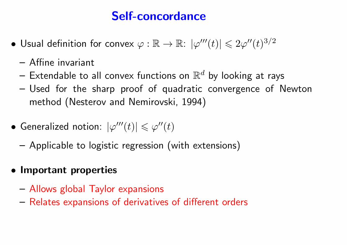
• Usual definition for convex ϕ : R → R: |ϕ′′′(t)| 6 2ϕ′′(t)3/2
– Affine invariant
– Extendable to all convex functions on Rd by looking at rays
– Used for the sharp proof of quadratic convergence of Newton
method (Nesterov and Nemirovski, 1994)
• Generalized notion: |ϕ′′′(t)| 6 ϕ′′(t)
– Applicable to logistic regression (with extensions)
• Important properties
– Allows global Taylor expansions
– Relates expansions of derivatives of different orders
Adaptive algorithm for logistic regression
Proof sketch
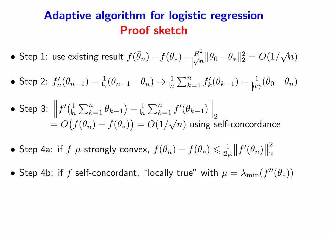
• Step 1: use existing result f(θn)−f(θ∗)+R2√n‖θ0−θ∗‖22 = O(1/
√n)
• Step 2: f ′n(θn−1) =
1γ(θn−1−θn) ⇒ 1
n
∑nk=1 f
′k(θk−1) =
1nγ(θ0−θn)
• Step 3:∥
∥
∥f ′(1
n
∑nk=1 θk−1
)
− 1n
∑nk=1 f
′(θk−1)∥
∥
∥
2
= O(
f(θn)− f(θ∗))
= O(1/√n) using self-concordance
• Step 4a: if f µ-strongly convex, f(θn)− f(θ∗) 612µ
∥
∥f ′(θn)∥
∥
2
2
• Step 4b: if f self-concordant, “locally true” with µ = λmin(f′′(θ∗))
Adaptive algorithm for logistic regression
• Logistic regression: (Φ(xn), yn) ∈ Rd × −1, 1
– Single data point: fn(θ) = log(1 + exp(−ynθ⊤Φ(xn)))
– Generalization error: f(θ) = Efn(θ)
• Cannot be strongly convex ⇒ local strong convexity
– unless restricted to |θ⊤Φ(xn)| 6 M (and with constants eM)
– µ = lowest eigenvalue of the Hessian at the optimum f ′′(θ∗)
• n steps of averaged SGD with constant step-size 1/(
2R2√n)
– with R = radius of data (Bach, 2013):
Ef(θn)− f(θ∗) 6 min
1√n,R2
nµ
(
15 + 5R‖θ0 − θ∗‖)4
– Proof based on self-concordance (Nesterov and Nemirovski, 1994)
Adaptive algorithm for logistic regression
• Logistic regression: (Φ(xn), yn) ∈ Rd × −1, 1
– Single data point: fn(θ) = log(1 + exp(−ynθ⊤Φ(xn)))
– Generalization error: f(θ) = Efn(θ)
• Cannot be strongly convex ⇒ local strong convexity
– unless restricted to |θ⊤Φ(xn)| 6 M (and with constants eM)
– µ = lowest eigenvalue of the Hessian at the optimum f ′′(θ∗)
• n steps of averaged SGD with constant step-size 1/(
2R2√n)
– with R = radius of data (Bach, 2013):
Ef(θn)− f(θ∗) 6 min
1√n,R2
nµ
(
15 + 5R‖θ0 − θ∗‖)4
– A single adaptive algorithm for smooth problems with
convergence rate O(1/n) in all situations?
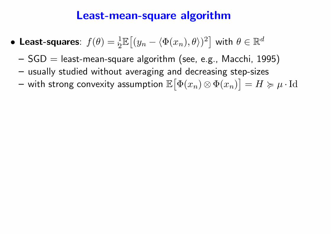
Least-mean-square algorithm
• Least-squares: f(θ) = 12E
[
(yn − 〈Φ(xn), θ〉)2]
with θ ∈ Rd
– SGD = least-mean-square algorithm (see, e.g., Macchi, 1995)
– usually studied without averaging and decreasing step-sizes
– with strong convexity assumption E[
Φ(xn)⊗Φ(xn)]
= H < µ · Id
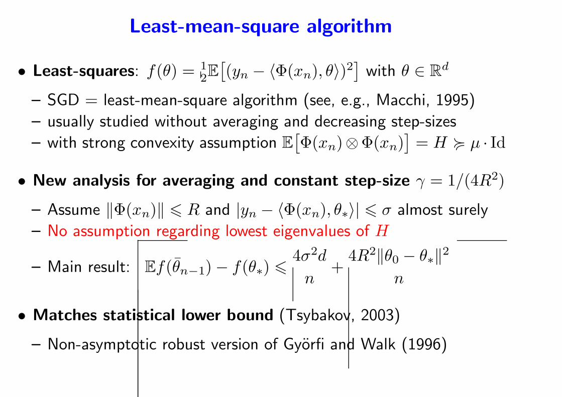
Least-mean-square algorithm
• Least-squares: f(θ) = 12E
[
(yn − 〈Φ(xn), θ〉)2]
with θ ∈ Rd
– SGD = least-mean-square algorithm (see, e.g., Macchi, 1995)
– usually studied without averaging and decreasing step-sizes
– with strong convexity assumption E[
Φ(xn)⊗Φ(xn)]
= H < µ · Id
• New analysis for averaging and constant step-size γ = 1/(4R2)
– Assume ‖Φ(xn)‖ 6 R and |yn − 〈Φ(xn), θ∗〉| 6 σ almost surely
– No assumption regarding lowest eigenvalues of H
– Main result: Ef(θn−1)− f(θ∗) 64σ2d
n+
4R2‖θ0 − θ∗‖2n
• Matches statistical lower bound (Tsybakov, 2003)
– Non-asymptotic robust version of Gyorfi and Walk (1996)
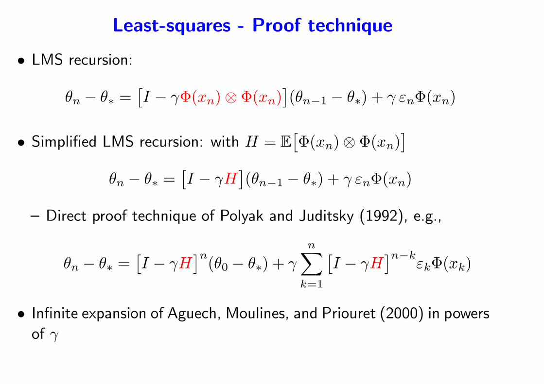
Least-squares - Proof technique
• LMS recursion:
θn − θ∗ =[
I − γΦ(xn)⊗ Φ(xn)]
(θn−1 − θ∗) + γ εnΦ(xn)
• Simplified LMS recursion: with H = E[
Φ(xn)⊗ Φ(xn)]
θn − θ∗ =[
I − γH]
(θn−1 − θ∗) + γ εnΦ(xn)
– Direct proof technique of Polyak and Juditsky (1992), e.g.,
θn − θ∗ =[
I − γH]n(θ0 − θ∗) + γ
n∑
k=1
[
I − γH]n−k
εkΦ(xk)
• Infinite expansion of Aguech, Moulines, and Priouret (2000) in powers
of γ
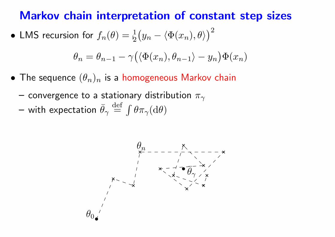
Markov chain interpretation of constant step sizes
• LMS recursion for fn(θ) =12
(
yn − 〈Φ(xn), θ〉)2
θn = θn−1 − γ(
〈Φ(xn), θn−1〉 − yn)
Φ(xn)
• The sequence (θn)n is a homogeneous Markov chain
– convergence to a stationary distribution πγ
– with expectation θγdef=
∫
θπγ(dθ)
- For least-squares, θγ = θ∗
θγ
θ0
θn
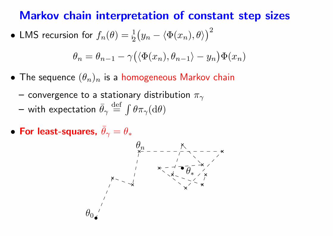
Markov chain interpretation of constant step sizes
• LMS recursion for fn(θ) =12
(
yn − 〈Φ(xn), θ〉)2
θn = θn−1 − γ(
〈Φ(xn), θn−1〉 − yn)
Φ(xn)
• The sequence (θn)n is a homogeneous Markov chain
– convergence to a stationary distribution πγ
– with expectation θγdef=
∫
θπγ(dθ)
• For least-squares, θγ = θ∗
θ∗
θ0
θn
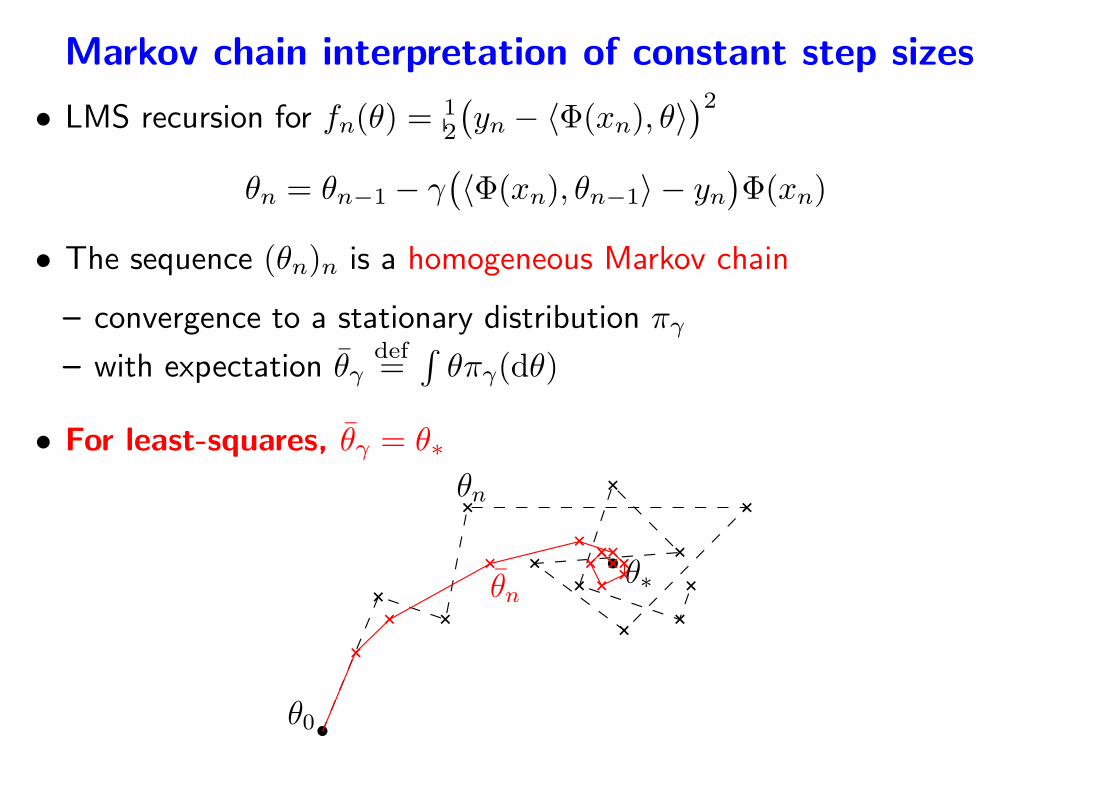
Markov chain interpretation of constant step sizes
• LMS recursion for fn(θ) =12
(
yn − 〈Φ(xn), θ〉)2
θn = θn−1 − γ(
〈Φ(xn), θn−1〉 − yn)
Φ(xn)
• The sequence (θn)n is a homogeneous Markov chain
– convergence to a stationary distribution πγ
– with expectation θγdef=
∫
θπγ(dθ)
• For least-squares, θγ = θ∗
θ∗
θ0
θn
θn
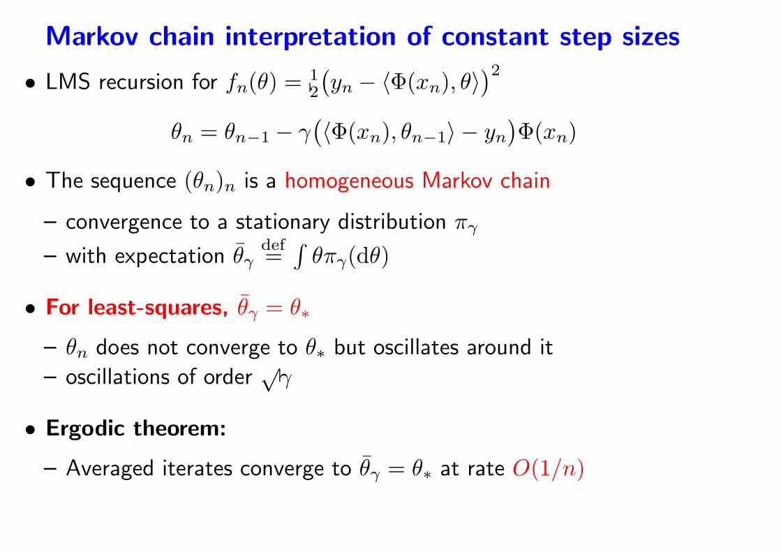
Markov chain interpretation of constant step sizes
• LMS recursion for fn(θ) =12
(
yn − 〈Φ(xn), θ〉)2
θn = θn−1 − γ(
〈Φ(xn), θn−1〉 − yn)
Φ(xn)
• The sequence (θn)n is a homogeneous Markov chain
– convergence to a stationary distribution πγ
– with expectation θγdef=
∫
θπγ(dθ)
• For least-squares, θγ = θ∗
– θn does not converge to θ∗ but oscillates around it
– oscillations of order√γ
• Ergodic theorem:
– Averaged iterates converge to θγ = θ∗ at rate O(1/n)
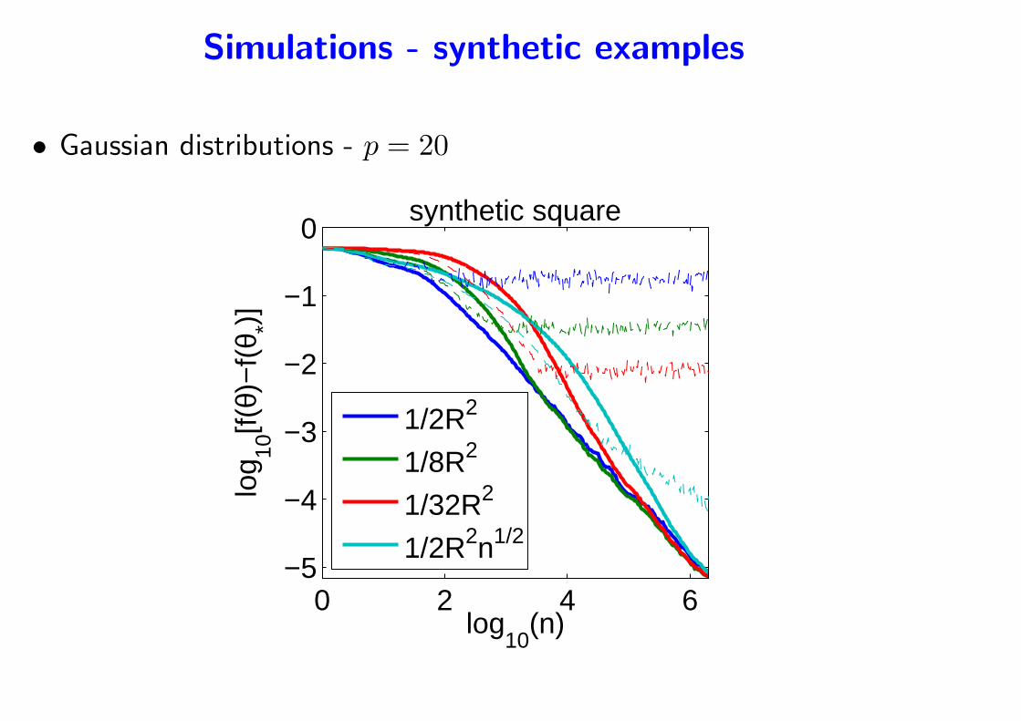
Simulations - synthetic examples
• Gaussian distributions - p = 20
0 2 4 6−5
−4
−3
−2
−1
0
log10
(n)
log 10
[f(θ)
−f(
θ *)]
synthetic square
1/2R2
1/8R2
1/32R2
1/2R2n1/2
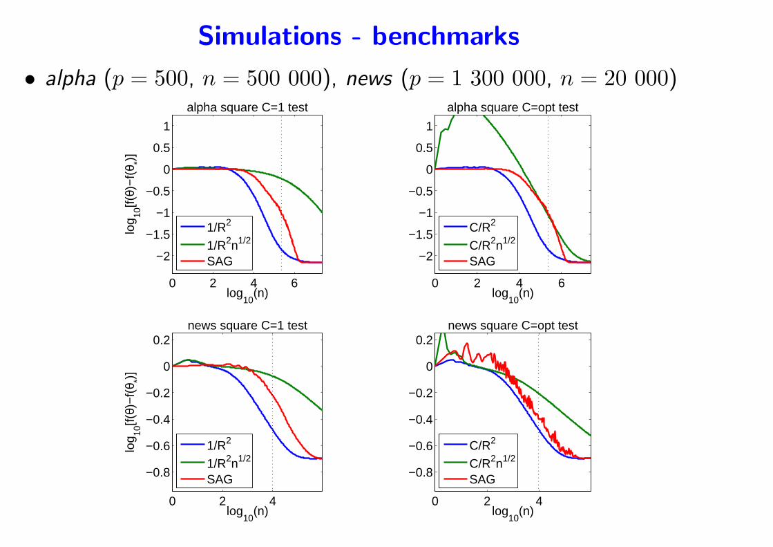
Simulations - benchmarks
• alpha (p = 500, n = 500 000), news (p = 1 300 000, n = 20 000)
0 2 4 6
−2
−1.5
−1
−0.5
0
0.5
1
log10
(n)
log 10
[f(θ)
−f(
θ *)]
alpha square C=1 test
1/R2
1/R2n1/2
SAG
0 2 4 6
−2
−1.5
−1
−0.5
0
0.5
1
log10
(n)
alpha square C=opt test
C/R2
C/R2n1/2
SAG
0 2 4
−0.8
−0.6
−0.4
−0.2
0
0.2
log10
(n)
log 10
[f(θ)
−f(
θ *)]
news square C=1 test
1/R2
1/R2n1/2
SAG
0 2 4
−0.8
−0.6
−0.4
−0.2
0
0.2
log10
(n)
news square C=opt test
C/R2
C/R2n1/2
SAG
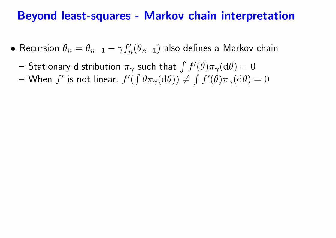
Beyond least-squares - Markov chain interpretation
• Recursion θn = θn−1 − γf ′n(θn−1) also defines a Markov chain
– Stationary distribution πγ such that∫
f ′(θ)πγ(dθ) = 0
– When f ′ is not linear, f ′(∫
θπγ(dθ)) 6=∫
f ′(θ)πγ(dθ) = 0
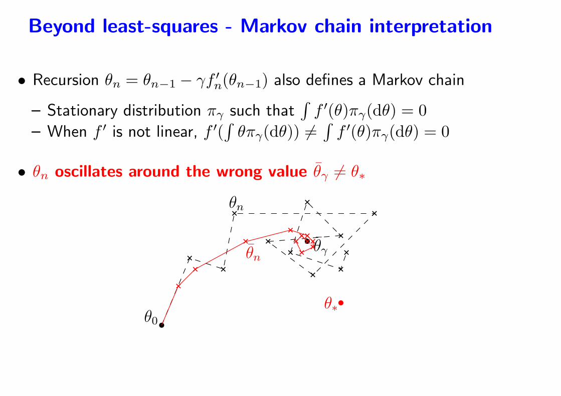
Beyond least-squares - Markov chain interpretation
• Recursion θn = θn−1 − γf ′n(θn−1) also defines a Markov chain
– Stationary distribution πγ such that∫
f ′(θ)πγ(dθ) = 0
– When f ′ is not linear, f ′(∫
θπγ(dθ)) 6=∫
f ′(θ)πγ(dθ) = 0
• θn oscillates around the wrong value θγ 6= θ∗
θγ
θ0
θn
θn
θ∗
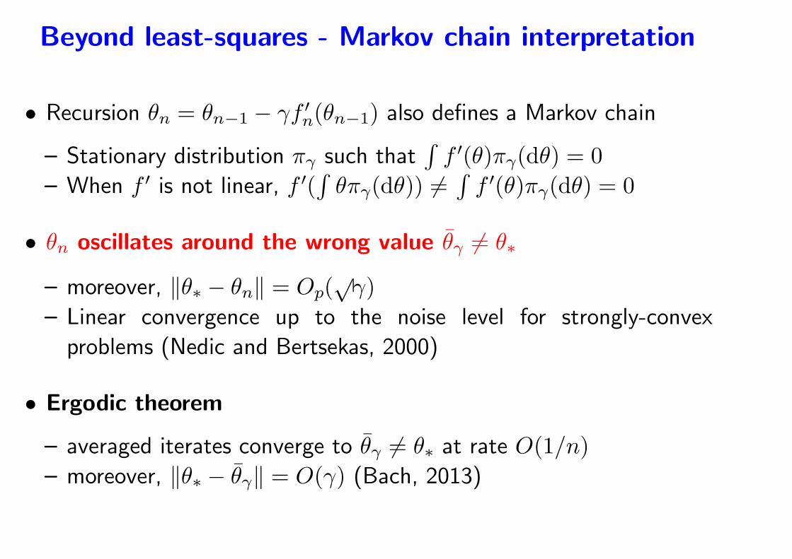
Beyond least-squares - Markov chain interpretation
• Recursion θn = θn−1 − γf ′n(θn−1) also defines a Markov chain
– Stationary distribution πγ such that∫
f ′(θ)πγ(dθ) = 0
– When f ′ is not linear, f ′(∫
θπγ(dθ)) 6=∫
f ′(θ)πγ(dθ) = 0
• θn oscillates around the wrong value θγ 6= θ∗
– moreover, ‖θ∗ − θn‖ = Op(√γ)
– Linear convergence up to the noise level for strongly-convex
problems (Nedic and Bertsekas, 2000)
• Ergodic theorem
– averaged iterates converge to θγ 6= θ∗ at rate O(1/n)
– moreover, ‖θ∗ − θγ‖ = O(γ) (Bach, 2013)
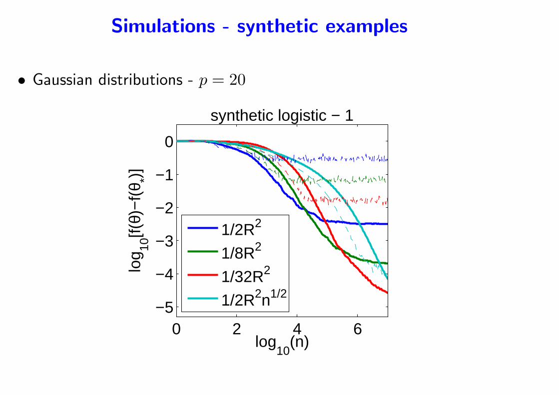
Simulations - synthetic examples
• Gaussian distributions - p = 20
0 2 4 6−5
−4
−3
−2
−1
0
log10
(n)
log 10
[f(θ)
−f(
θ *)]
synthetic logistic − 1
1/2R2
1/8R2
1/32R2
1/2R2n1/2
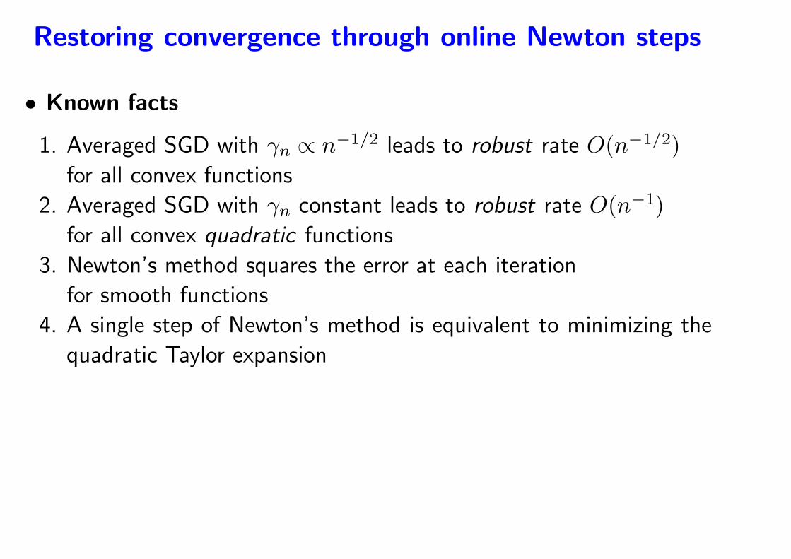
Restoring convergence through online Newton steps
• Known facts
1. Averaged SGD with γn ∝ n−1/2 leads to robust rate O(n−1/2)
for all convex functions
2. Averaged SGD with γn constant leads to robust rate O(n−1)
for all convex quadratic functions
3. Newton’s method squares the error at each iteration
for smooth functions
4. A single step of Newton’s method is equivalent to minimizing the
quadratic Taylor expansion
– Online Newton step
– Rate: O((n−1/2)2 + n−1) = O(n−1)
– Complexity: O(p) per iteration
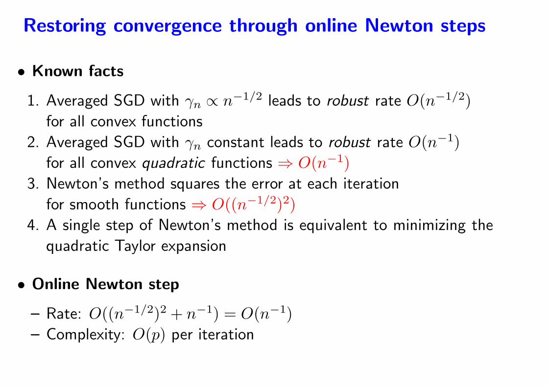
Restoring convergence through online Newton steps
• Known facts
1. Averaged SGD with γn ∝ n−1/2 leads to robust rate O(n−1/2)
for all convex functions
2. Averaged SGD with γn constant leads to robust rate O(n−1)
for all convex quadratic functions ⇒ O(n−1)
3. Newton’s method squares the error at each iteration
for smooth functions ⇒ O((n−1/2)2)
4. A single step of Newton’s method is equivalent to minimizing the
quadratic Taylor expansion
• Online Newton step
– Rate: O((n−1/2)2 + n−1) = O(n−1)
– Complexity: O(p) per iteration
Restoring convergence through online Newton steps
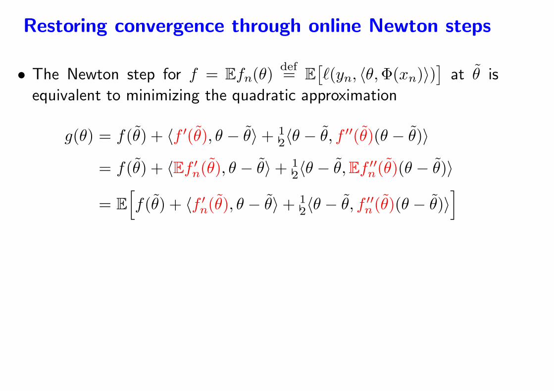
• The Newton step for f = Efn(θ)def= E
[
ℓ(yn, 〈θ,Φ(xn)〉)]
at θ is
equivalent to minimizing the quadratic approximation
g(θ) = f(θ) + 〈f ′(θ), θ − θ〉+ 12〈θ − θ, f ′′(θ)(θ − θ)〉
= f(θ) + 〈Ef ′n(θ), θ − θ〉+ 1
2〈θ − θ,Ef ′′n(θ)(θ − θ)〉
= E
[
f(θ) + 〈f ′n(θ), θ − θ〉+ 1
2〈θ − θ, f ′′n(θ)(θ − θ)〉
]
Restoring convergence through online Newton steps
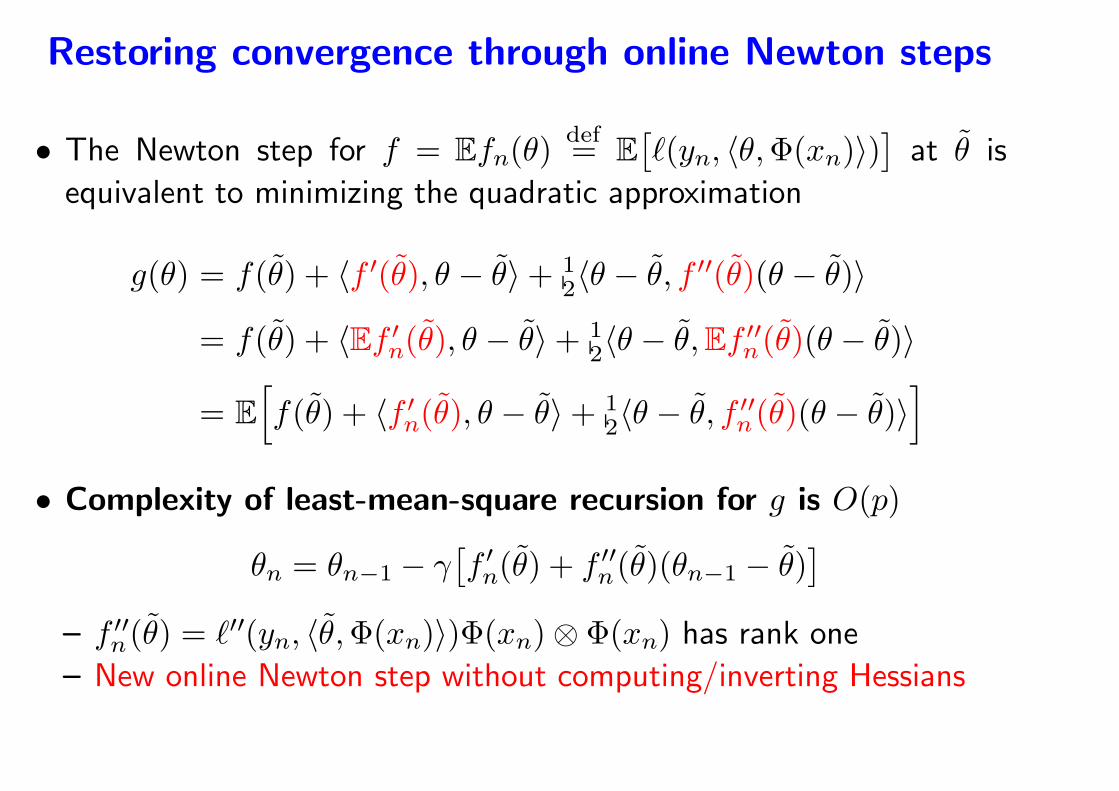
• The Newton step for f = Efn(θ)def= E
[
ℓ(yn, 〈θ,Φ(xn)〉)]
at θ is
equivalent to minimizing the quadratic approximation
g(θ) = f(θ) + 〈f ′(θ), θ − θ〉+ 12〈θ − θ, f ′′(θ)(θ − θ)〉
= f(θ) + 〈Ef ′n(θ), θ − θ〉+ 1
2〈θ − θ,Ef ′′n(θ)(θ − θ)〉
= E
[
f(θ) + 〈f ′n(θ), θ − θ〉+ 1
2〈θ − θ, f ′′n(θ)(θ − θ)〉
]
• Complexity of least-mean-square recursion for g is O(p)
θn = θn−1 − γ[
f ′n(θ) + f ′′
n(θ)(θn−1 − θ)]
– f ′′n(θ) = ℓ′′(yn, 〈θ,Φ(xn)〉)Φ(xn)⊗ Φ(xn) has rank one
– New online Newton step without computing/inverting Hessians
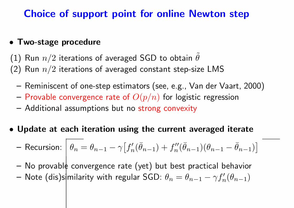
Choice of support point for online Newton step
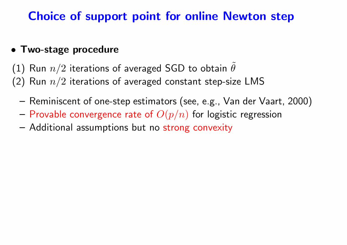
• Two-stage procedure
(1) Run n/2 iterations of averaged SGD to obtain θ
(2) Run n/2 iterations of averaged constant step-size LMS
– Reminiscent of one-step estimators (see, e.g., Van der Vaart, 2000)
– Provable convergence rate of O(p/n) for logistic regression
– Additional assumptions but no strong convexity
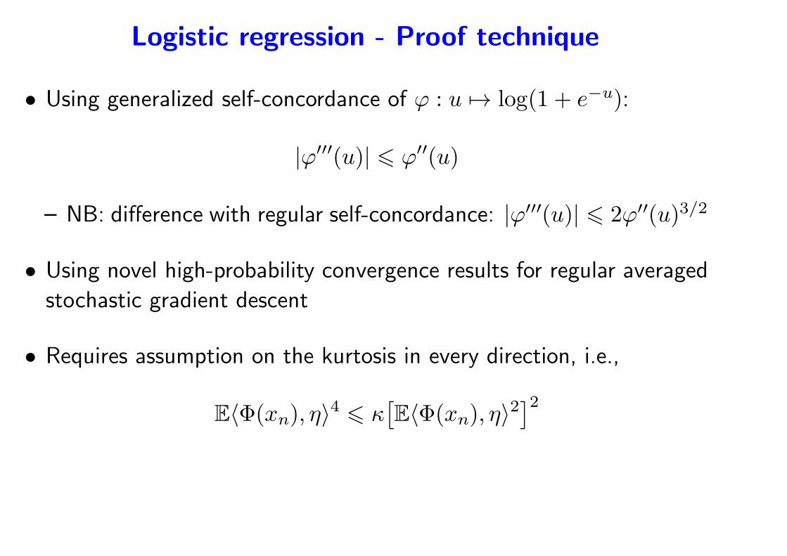
Logistic regression - Proof technique
• Using generalized self-concordance of ϕ : u 7→ log(1 + e−u):
|ϕ′′′(u)| 6 ϕ′′(u)
– NB: difference with regular self-concordance: |ϕ′′′(u)| 6 2ϕ′′(u)3/2
• Using novel high-probability convergence results for regular averaged
stochastic gradient descent
• Requires assumption on the kurtosis in every direction, i.e.,
E〈Φ(xn), η〉4 6 κ[
E〈Φ(xn), η〉2]2
Choice of support point for online Newton step
• Two-stage procedure
(1) Run n/2 iterations of averaged SGD to obtain θ
(2) Run n/2 iterations of averaged constant step-size LMS
– Reminiscent of one-step estimators (see, e.g., Van der Vaart, 2000)
– Provable convergence rate of O(p/n) for logistic regression
– Additional assumptions but no strong convexity
• Update at each iteration using the current averaged iterate
– Recursion: θn = θn−1 − γ[
f ′n(θn−1) + f ′′
n(θn−1)(θn−1 − θn−1)]
– No provable convergence rate (yet) but best practical behavior
– Note (dis)similarity with regular SGD: θn = θn−1 − γf ′n(θn−1)
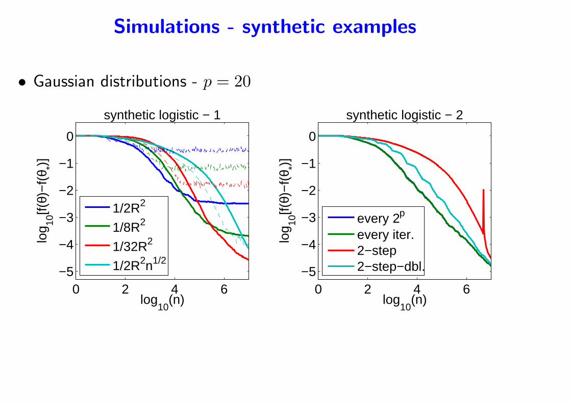
Simulations - synthetic examples
• Gaussian distributions - p = 20
0 2 4 6−5
−4
−3
−2
−1
0
log10
(n)
log 10
[f(θ)
−f(
θ *)]
synthetic logistic − 1
1/2R2
1/8R2
1/32R2
1/2R2n1/2
0 2 4 6−5
−4
−3
−2
−1
0
log10
(n)lo
g 10[f(
θ)−
f(θ *)]
synthetic logistic − 2
every 2p
every iter.2−step2−step−dbl.
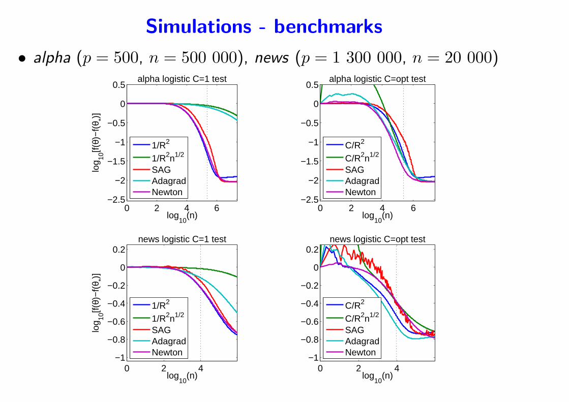
Simulations - benchmarks
• alpha (p = 500, n = 500 000), news (p = 1 300 000, n = 20 000)
0 2 4 6−2.5
−2
−1.5
−1
−0.5
0
0.5
log10
(n)
log 10
[f(θ)
−f(
θ *)]
alpha logistic C=1 test
1/R2
1/R2n1/2
SAGAdagradNewton
0 2 4 6−2.5
−2
−1.5
−1
−0.5
0
0.5
log10
(n)
alpha logistic C=opt test
C/R2
C/R2n1/2
SAGAdagradNewton
0 2 4−1
−0.8
−0.6
−0.4
−0.2
0
0.2
log10
(n)
log 10
[f(θ)
−f(
θ *)]
news logistic C=1 test
1/R2
1/R2n1/2
SAGAdagradNewton
0 2 4−1
−0.8
−0.6
−0.4
−0.2
0
0.2
log10
(n)
news logistic C=opt test
C/R2
C/R2n1/2
SAGAdagradNewton
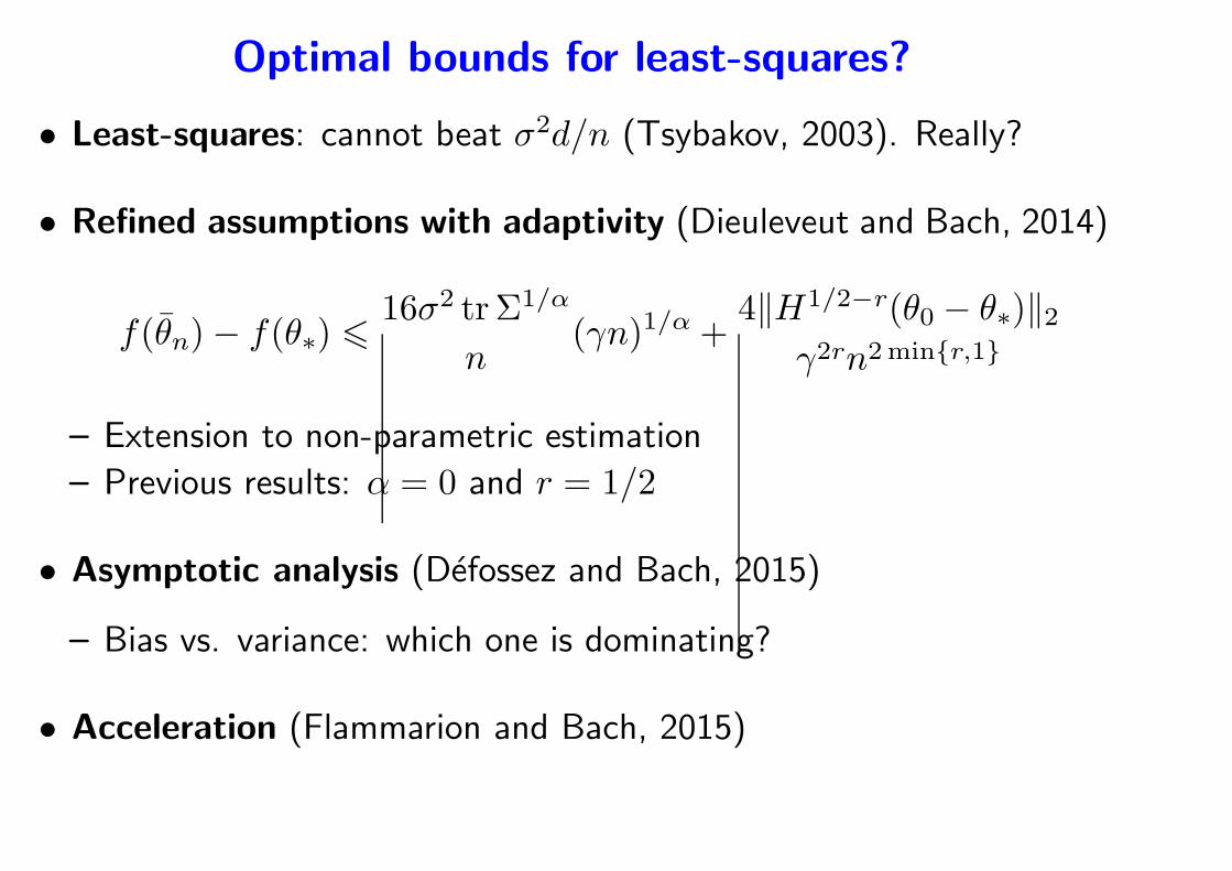
Optimal bounds for least-squares?
• Least-squares: cannot beat σ2d/n (Tsybakov, 2003). Really?
• Refined assumptions with adaptivity (Dieuleveut and Bach, 2014)
f(θn)− f(θ∗) 616σ2 tr Σ1/α
n(γn)1/α +
4‖H1/2−r(θ0 − θ∗)‖2γ2rn2minr,1
– Extension to non-parametric estimation
– Previous results: α = 0 and r = 1/2
• Asymptotic analysis (Defossez and Bach, 2015)
– Bias vs. variance: which one is dominating?
• Acceleration (Flammarion and Bach, 2015)
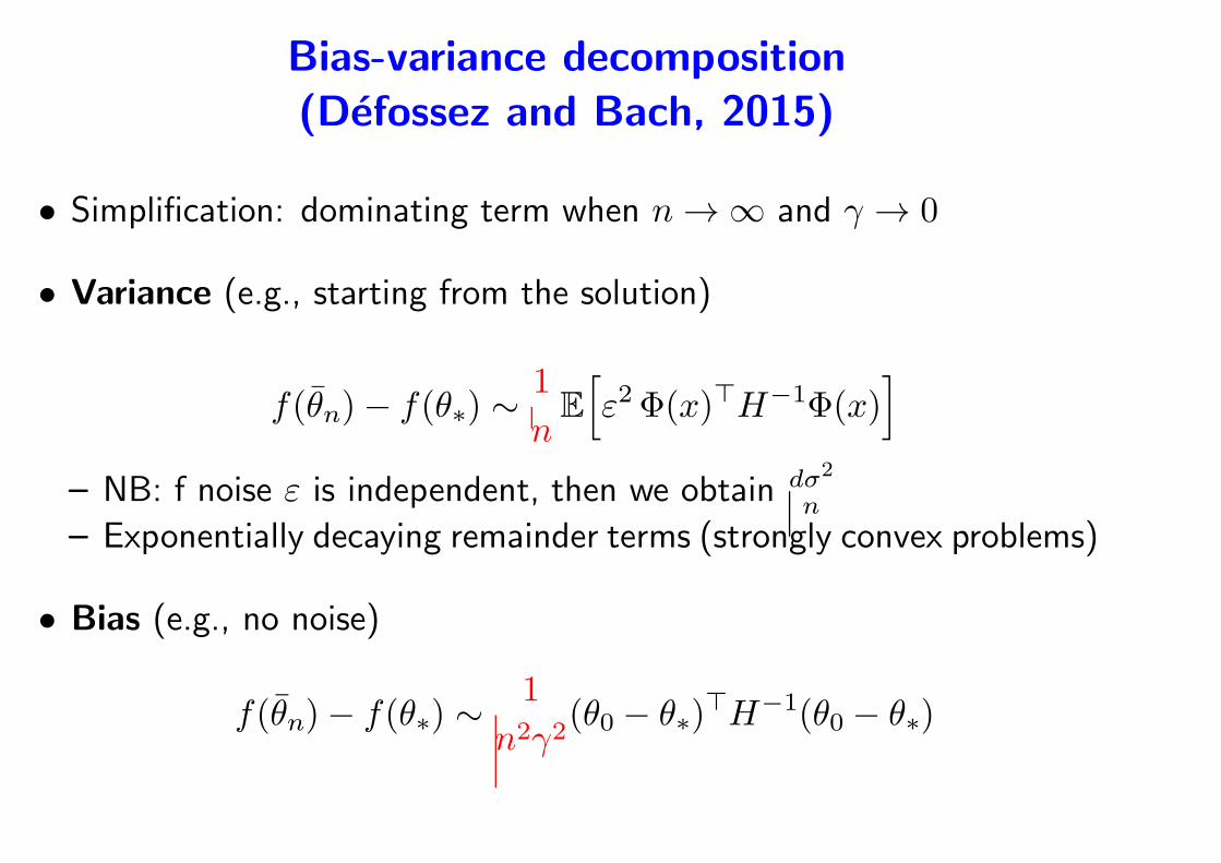
Bias-variance decomposition
(Defossez and Bach, 2015)
• Simplification: dominating term when n → ∞ and γ → 0
• Variance (e.g., starting from the solution)
f(θn)− f(θ∗) ∼1
nE
[
ε2Φ(x)⊤H−1Φ(x)]
– NB: f noise ε is independent, then we obtain dσ2
n
– Exponentially decaying remainder terms (strongly convex problems)
• Bias (e.g., no noise)
f(θn)− f(θ∗) ∼1
n2γ2(θ0 − θ∗)
⊤H−1(θ0 − θ∗)
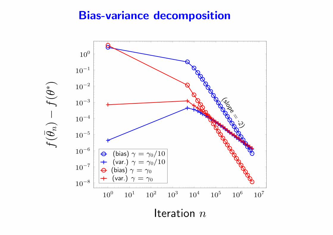
Bias-variance decomposition
100 101 102 103 104 105 106 107
10−8
10−7
10−6
10−5
10−4
10−3
10−2
10−1
100
(slope=-2)
Iteration n
f(θ
n)−
f(θ
∗ )
(bias) γ = γ0/10(var.) γ = γ0/10(bias) γ = γ0
(var.) γ = γ0
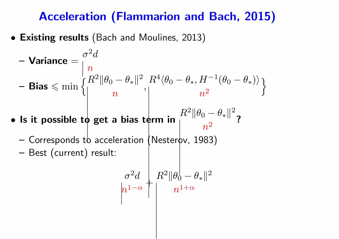
Acceleration (Flammarion and Bach, 2015)
• Existing results (Bach and Moulines, 2013)
– Variance =σ2d
n
– Bias 6 minR2‖θ0 − θ∗‖2
n,R4〈θ0 − θ∗,H−1(θ0 − θ∗)〉
n2
• Is it possible to get a bias term inR2‖θ0 − θ∗‖2
n2?
– Corresponds to acceleration (Nesterov, 1983)
– Best (current) result:
σ2d
n1−α+
R2‖θ0 − θ∗‖2n1+α
Outline
1. Large-scale machine learning and optimization
• Traditional statistical analysis
• Classical methods for convex optimization
2. Non-smooth stochastic approximation
• Stochastic (sub)gradient and averaging
• Non-asymptotic results and lower bounds
• Strongly convex vs. non-strongly convex
3. Smooth stochastic approximation algorithms
• Asymptotic and non-asymptotic results
• Beyond decaying step-sizes
4. Finite data sets
Going beyond a single pass over the data
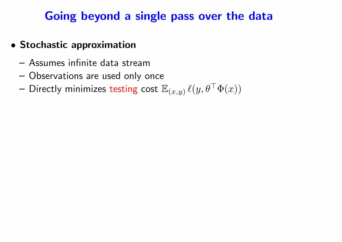
• Stochastic approximation
– Assumes infinite data stream
– Observations are used only once
– Directly minimizes testing cost E(x,y) ℓ(y, θ⊤Φ(x))
Going beyond a single pass over the data
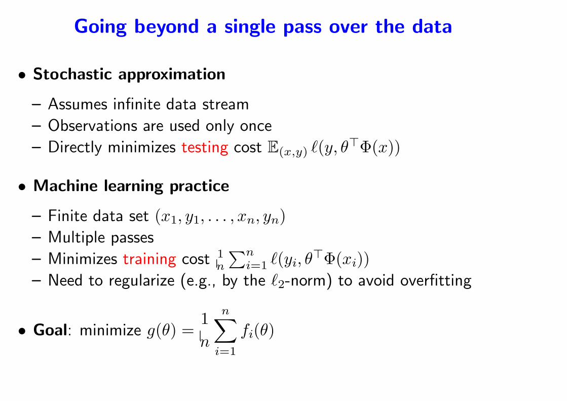
• Stochastic approximation
– Assumes infinite data stream
– Observations are used only once
– Directly minimizes testing cost E(x,y) ℓ(y, θ⊤Φ(x))
• Machine learning practice
– Finite data set (x1, y1, . . . , xn, yn)
– Multiple passes
– Minimizes training cost 1n
∑ni=1 ℓ(yi, θ
⊤Φ(xi))
– Need to regularize (e.g., by the ℓ2-norm) to avoid overfitting
• Goal: minimize g(θ) =1
n
n∑
i=1
fi(θ)
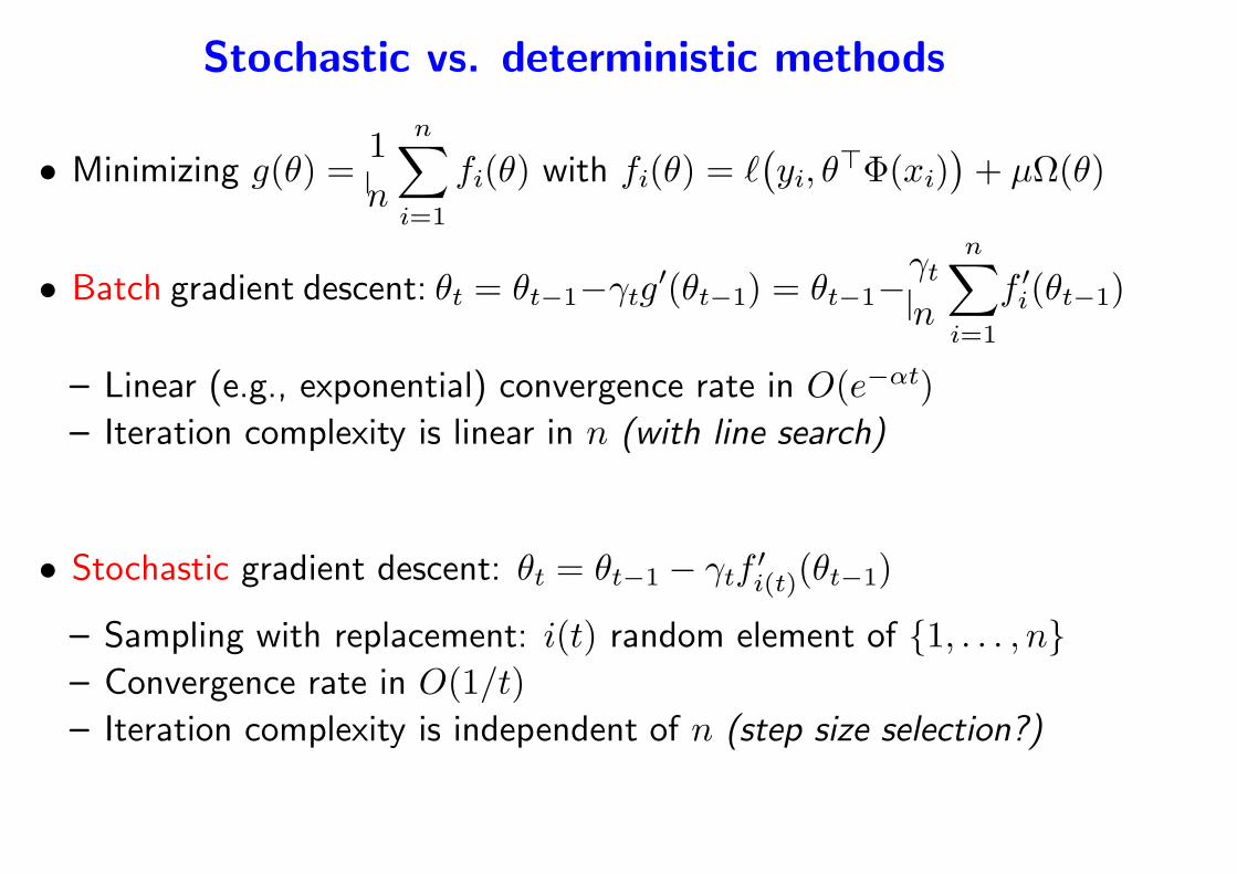
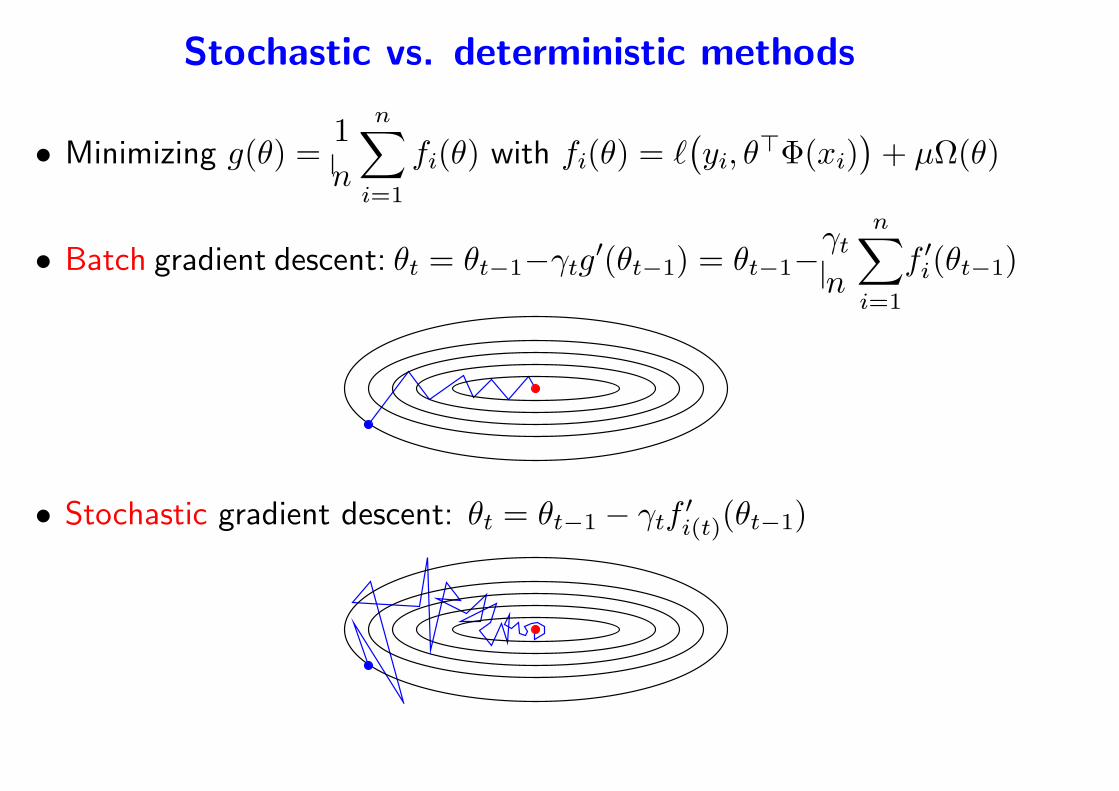
Stochastic vs. deterministic methods
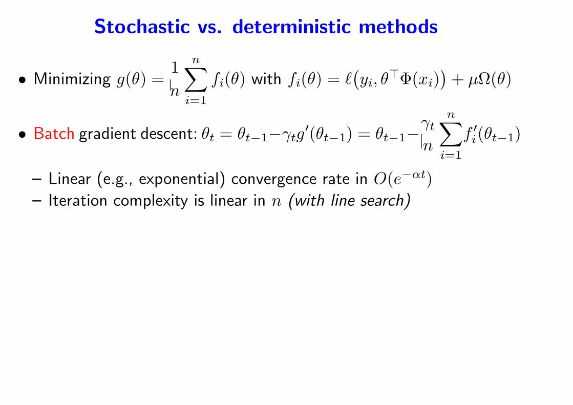
• Minimizing g(θ) =1
n
n∑
i=1
fi(θ) with fi(θ) = ℓ(
yi, θ⊤Φ(xi)
)
+ µΩ(θ)
• Batch gradient descent: θt = θt−1−γtg′(θt−1) = θt−1−
γtn
n∑
i=1
f ′i(θt−1)
– Linear (e.g., exponential) convergence rate in O(e−αt)
– Iteration complexity is linear in n (with line search)
Stochastic vs. deterministic methods
• Minimizing g(θ) =1
n
n∑
i=1
fi(θ) with fi(θ) = ℓ(
yi, θ⊤Φ(xi)
)
+ µΩ(θ)
• Batch gradient descent: θt = θt−1−γtg′(θt−1) = θt−1−
γtn
n∑
i=1
f ′i(θt−1)
Stochastic vs. deterministic methods
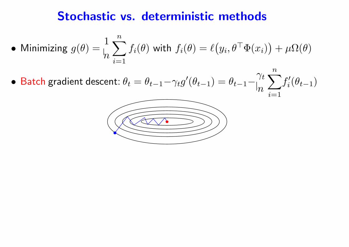
• Minimizing g(θ) =1
n
n∑
i=1
fi(θ) with fi(θ) = ℓ(
yi, θ⊤Φ(xi)
)
+ µΩ(θ)
• Batch gradient descent: θt = θt−1−γtg′(θt−1) = θt−1−
γtn
n∑
i=1
f ′i(θt−1)
– Linear (e.g., exponential) convergence rate in O(e−αt)
– Iteration complexity is linear in n (with line search)
• Stochastic gradient descent: θt = θt−1 − γtf′i(t)(θt−1)
– Sampling with replacement: i(t) random element of 1, . . . , n– Convergence rate in O(1/t)
– Iteration complexity is independent of n (step size selection?)
Stochastic vs. deterministic methods
• Minimizing g(θ) =1
n
n∑
i=1
fi(θ) with fi(θ) = ℓ(
yi, θ⊤Φ(xi)
)
+ µΩ(θ)
• Batch gradient descent: θt = θt−1−γtg′(θt−1) = θt−1−
γtn
n∑
i=1
f ′i(θt−1)
• Stochastic gradient descent: θt = θt−1 − γtf′i(t)(θt−1)
Stochastic vs. deterministic methods
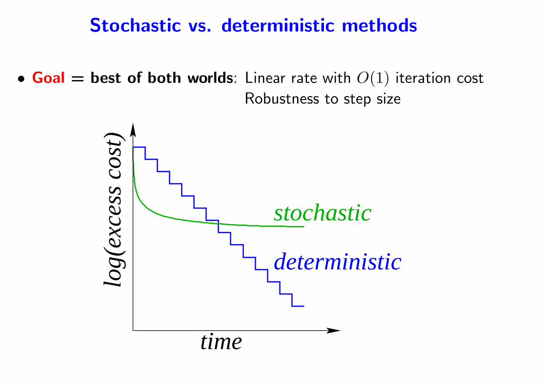
• Goal = best of both worlds: Linear rate with O(1) iteration cost
Robustness to step size
time
log
(exc
ess
co
st)
stochastic
deterministic
Stochastic vs. deterministic methods
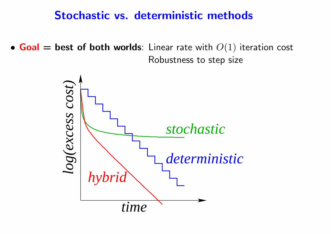
• Goal = best of both worlds: Linear rate with O(1) iteration cost
Robustness to step size
hybridlog
(exc
ess
co
st)
stochastic
deterministic
time
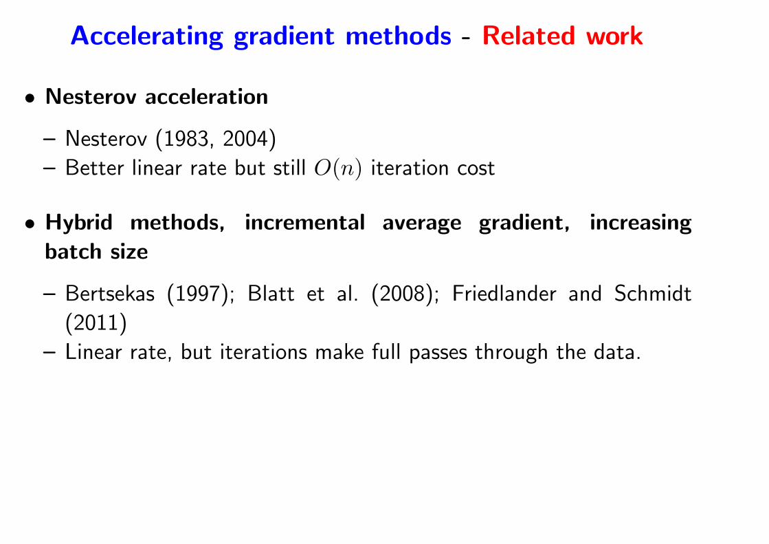
Accelerating gradient methods - Related work
• Nesterov acceleration
– Nesterov (1983, 2004)
– Better linear rate but still O(n) iteration cost
• Hybrid methods, incremental average gradient, increasing
batch size
– Bertsekas (1997); Blatt et al. (2008); Friedlander and Schmidt
(2011)
– Linear rate, but iterations make full passes through the data.
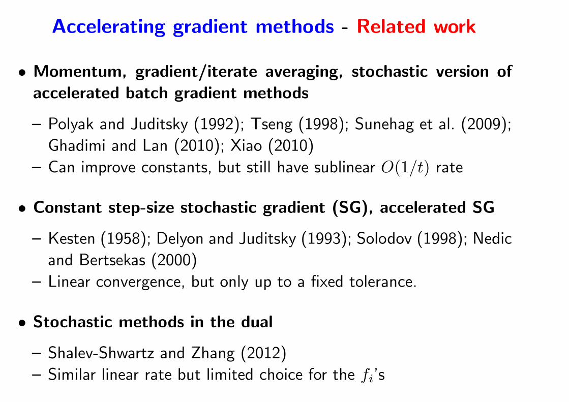
Accelerating gradient methods - Related work
• Momentum, gradient/iterate averaging, stochastic version of
accelerated batch gradient methods
– Polyak and Juditsky (1992); Tseng (1998); Sunehag et al. (2009);
Ghadimi and Lan (2010); Xiao (2010)
– Can improve constants, but still have sublinear O(1/t) rate
• Constant step-size stochastic gradient (SG), accelerated SG
– Kesten (1958); Delyon and Juditsky (1993); Solodov (1998); Nedic
and Bertsekas (2000)
– Linear convergence, but only up to a fixed tolerance.
• Stochastic methods in the dual
– Shalev-Shwartz and Zhang (2012)
– Similar linear rate but limited choice for the fi’s
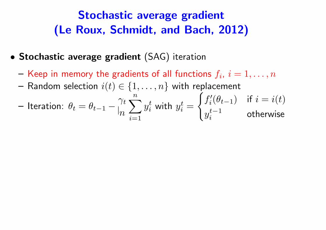
Stochastic average gradient
(Le Roux, Schmidt, and Bach, 2012)
• Stochastic average gradient (SAG) iteration
– Keep in memory the gradients of all functions fi, i = 1, . . . , n
– Random selection i(t) ∈ 1, . . . , n with replacement
– Iteration: θt = θt−1 −γtn
n∑
i=1
yti with yti =
f ′i(θt−1) if i = i(t)
yt−1i otherwise
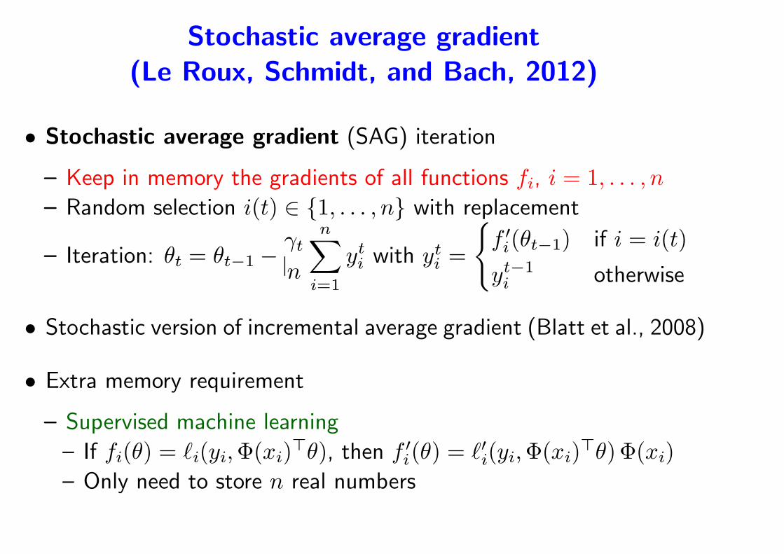
• Stochastic version of incremental average gradient (Blatt et al., 2008)
• Extra memory requirement
– Supervised machine learning
– If fi(θ) = ℓi(yi,Φ(xi)⊤θ), then f ′
i(θ) = ℓ′i(yi,Φ(xi)⊤θ)Φ(xi)
– Only need to store n real numbers
Stochastic average gradient - Convergence analysis
• Assumptions
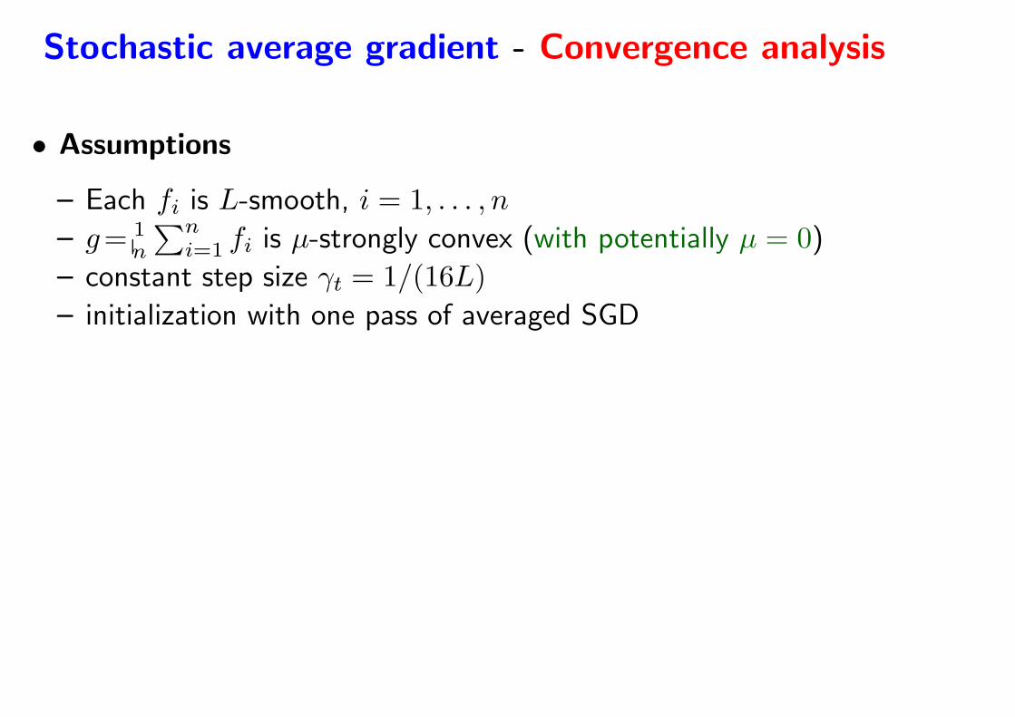
– Each fi is L-smooth, i = 1, . . . , n
– g= 1n
∑ni=1 fi is µ-strongly convex (with potentially µ = 0)
– constant step size γt = 1/(16L)
– initialization with one pass of averaged SGD
Stochastic average gradient - Convergence analysis
• Assumptions
– Each fi is L-smooth, i = 1, . . . , n
– g= 1n
∑ni=1 fi is µ-strongly convex (with potentially µ = 0)
– constant step size γt = 1/(16L)
– initialization with one pass of averaged SGD
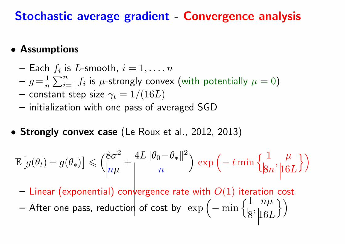
• Strongly convex case (Le Roux et al., 2012, 2013)
E[
g(θt)− g(θ∗)]
6
(8σ2
nµ+
4L‖θ0−θ∗‖2n
)
exp(
− tmin 1
8n,
µ
16L
)
– Linear (exponential) convergence rate with O(1) iteration cost
– After one pass, reduction of cost by exp(
−min1
8,nµ
16L
)
Stochastic average gradient - Convergence analysis
• Assumptions
– Each fi is L-smooth, i = 1, . . . , n
– g= 1n
∑ni=1 fi is µ-strongly convex (with potentially µ = 0)
– constant step size γt = 1/(16L)
– initialization with one pass of averaged SGD
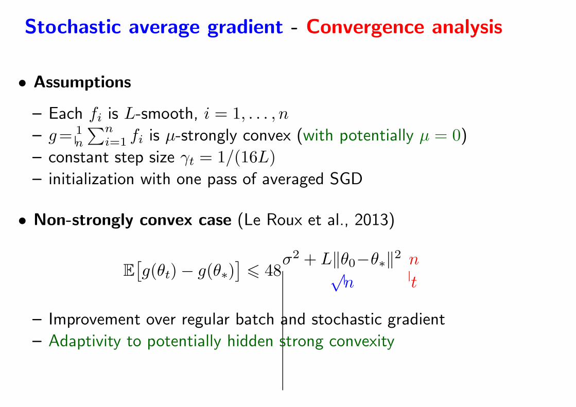
• Non-strongly convex case (Le Roux et al., 2013)
E[
g(θt)− g(θ∗)]
6 48σ2 + L‖θ0−θ∗‖2√
n
n
t
– Improvement over regular batch and stochastic gradient
– Adaptivity to potentially hidden strong convexity
Convergence analysis - Proof sketch
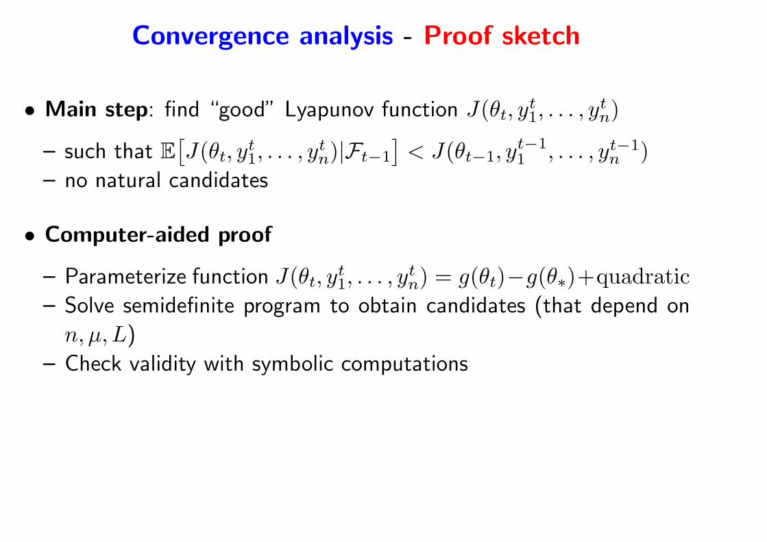
• Main step: find “good” Lyapunov function J(θt, yt1, . . . , y
tn)
– such that E[
J(θt, yt1, . . . , y
tn)|Ft−1
]
< J(θt−1, yt−11 , . . . , yt−1
n )
– no natural candidates
• Computer-aided proof
– Parameterize function J(θt, yt1, . . . , y
tn) = g(θt)−g(θ∗)+quadratic
– Solve semidefinite program to obtain candidates (that depend on
n, µ, L)
– Check validity with symbolic computations
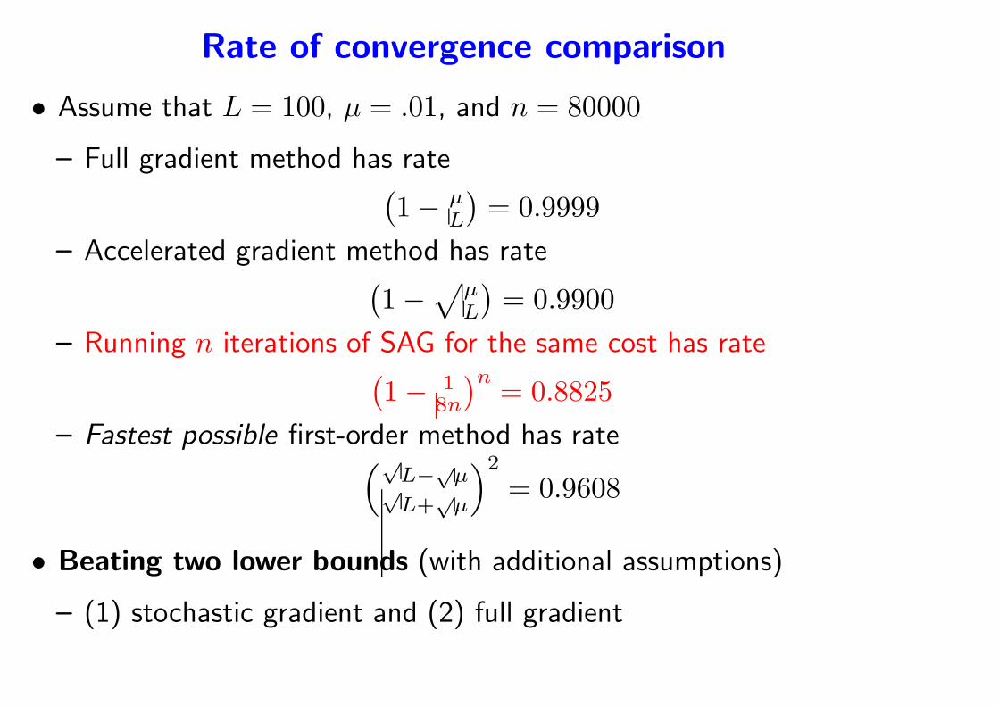
Rate of convergence comparison
• Assume that L = 100, µ = .01, and n = 80000
– Full gradient method has rate(
1− µL
)
= 0.9999
– Accelerated gradient method has rate(
1−√
µL
)
= 0.9900
– Running n iterations of SAG for the same cost has rate(
1− 18n
)n= 0.8825
– Fastest possible first-order method has rate(√
L−√µ√
L+õ
)2
= 0.9608
• Beating two lower bounds (with additional assumptions)
– (1) stochastic gradient and (2) full gradient
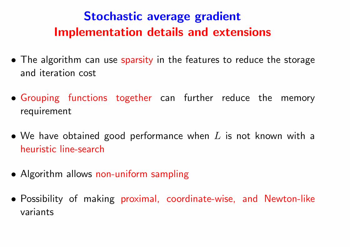
Stochastic average gradient
Implementation details and extensions
• The algorithm can use sparsity in the features to reduce the storage
and iteration cost
• Grouping functions together can further reduce the memory
requirement
• We have obtained good performance when L is not known with a
heuristic line-search
• Algorithm allows non-uniform sampling
• Possibility of making proximal, coordinate-wise, and Newton-like
variants
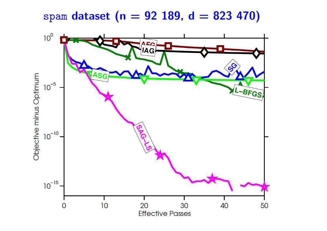
spam dataset (n = 92 189, d = 823 470)
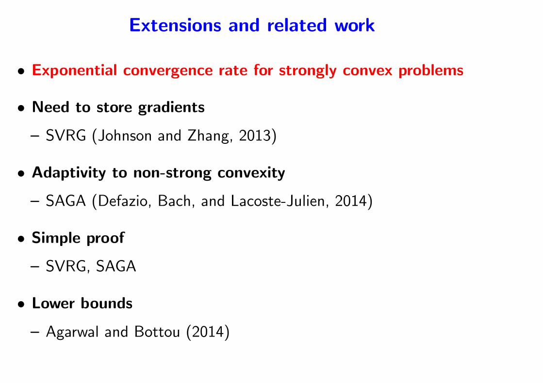
Extensions and related work
• Exponential convergence rate for strongly convex problems
• Need to store gradients
– SVRG (Johnson and Zhang, 2013)
• Adaptivity to non-strong convexity
– SAGA (Defazio, Bach, and Lacoste-Julien, 2014)
• Simple proof
– SVRG, SAGA
• Lower bounds
– Agarwal and Bottou (2014)
Summary and future work
• Constant-step-size averaged stochastic gradient descent
– Reaches convergence rate O(1/n) in all regimes
– Improves on the O(1/√n) lower-bound of non-smooth problems
– Efficient online Newton step for non-quadratic problems
– Robustness to step-size selection
• Going beyond a single pass through the data
• Extensions and future work
– Pre-conditioning
– Proximal extensions fo non-differentiable terms
– kernels and non-parametric estimation
– line-search
– parallelization

Outline
1. Large-scale machine learning and optimization
• Traditional statistical analysis
• Classical methods for convex optimization
2. Non-smooth stochastic approximation
• Stochastic (sub)gradient and averaging
• Non-asymptotic results and lower bounds
• Strongly convex vs. non-strongly convex
3. Smooth stochastic approximation algorithms
• Asymptotic and non-asymptotic results
• Beyond decaying step-sizes
4. Finite data sets
Conclusions
Machine learning and convex optimization
• Statistics with or without optimization?
– Significance of mixing algorithms with analysis
– Benefits of mixing algorithms with analysis
• Open problems
– Non-parametric stochastic approximation
– Going beyond a single pass over the data (testing performance)
– Characterization of implicit regularization of online methods
– Distributed processing
References
A. Agarwal, P. L. Bartlett, P. Ravikumar, and M. J. Wainwright. Information-theoretic lower bounds
on the oracle complexity of stochastic convex optimization. Information Theory, IEEE Transactions
on, 58(5):3235–3249, 2012.
Alekh Agarwal and Leon Bottou. A lower bound for the optimization of finite sums. arXiv preprint
arXiv:1410.0723, 2014.
R. Aguech, E. Moulines, and P. Priouret. On a perturbation approach for the analysis of stochastic
tracking algorithms. SIAM J. Control and Optimization, 39(3):872–899, 2000.
F. Bach. Adaptivity of averaged stochastic gradient descent to local strong convexity for logistic
regression. Technical Report 00804431, HAL, 2013.
F. Bach and E. Moulines. Non-asymptotic analysis of stochastic approximation algorithms for machine
learning. In Adv. NIPS, 2011.
F. Bach and E. Moulines. Non-strongly-convex smooth stochastic approximation with convergence
rate o(1/n). Technical Report 00831977, HAL, 2013.
F. Bach, R. Jenatton, J. Mairal, and G. Obozinski. Structured sparsity through convex optimization,
2012a.
Francis Bach, Rodolphe Jenatton, Julien Mairal, and Guillaume Obozinski. Optimization with sparsity-
inducing penalties. Foundations and Trends R© in Machine Learning, 4(1):1–106, 2012b.
A. Beck and M. Teboulle. A fast iterative shrinkage-thresholding algorithm for linear inverse problems.
SIAM Journal on Imaging Sciences, 2(1):183–202, 2009.
Albert Benveniste, Michel Metivier, and Pierre Priouret. Adaptive algorithms and stochastic
approximations. Springer Publishing Company, Incorporated, 2012.
D. P. Bertsekas. A new class of incremental gradient methods for least squares problems. SIAM
Journal on Optimization, 7(4):913–926, 1997.
D. Blatt, A. O. Hero, and H. Gauchman. A convergent incremental gradient method with a constant
step size. SIAM Journal on Optimization, 18(1):29–51, 2008.
L. Bottou and O. Bousquet. The tradeoffs of large scale learning. In Adv. NIPS, 2008.
L. Bottou and Y. Le Cun. On-line learning for very large data sets. Applied Stochastic Models in
Business and Industry, 21(2):137–151, 2005.
S. Boucheron and P. Massart. A high-dimensional wilks phenomenon. Probability theory and related
fields, 150(3-4):405–433, 2011.
S. Boucheron, O. Bousquet, G. Lugosi, et al. Theory of classification: A survey of some recent
advances. ESAIM Probability and statistics, 9:323–375, 2005.
N. Cesa-Bianchi, A. Conconi, and C. Gentile. On the generalization ability of on-line learning algorithms.
Information Theory, IEEE Transactions on, 50(9):2050–2057, 2004.
Aaron Defazio, Francis Bach, and Simon Lacoste-Julien. Saga: A fast incremental gradient method
with support for non-strongly convex composite objectives. In Advances in Neural Information
Processing Systems, pages 1646–1654, 2014.
A. Defossez and F. Bach. Constant step size least-mean-square: Bias-variance trade-offs and optimal
sampling distributions. 2015.
B. Delyon and A. Juditsky. Accelerated stochastic approximation. SIAM Journal on Optimization, 3:
868–881, 1993.
A. Dieuleveut and F. Bach. Non-parametric Stochastic Approximation with Large Step sizes. Technical
report, ArXiv, 2014.
J. Duchi and Y. Singer. Efficient online and batch learning using forward backward splitting. Journal
of Machine Learning Research, 10:2899–2934, 2009. ISSN 1532-4435.
N. Flammarion and F. Bach. From averaging to acceleration, there is only a step-size. arXiv preprint
arXiv:1504.01577, 2015.
M. P. Friedlander and M. Schmidt. Hybrid deterministic-stochastic methods for data fitting.
arXiv:1104.2373, 2011.
S. Ghadimi and G. Lan. Optimal stochastic approximation algorithms for strongly convex stochastic
composite optimization. Optimization Online, July, 2010.
Saeed Ghadimi and Guanghui Lan. Optimal stochastic approximation algorithms for strongly convex
stochastic composite optimization, ii: shrinking procedures and optimal algorithms. SIAM Journal
on Optimization, 23(4):2061–2089, 2013.
L. Gyorfi and H. Walk. On the averaged stochastic approximation for linear regression. SIAM Journal
on Control and Optimization, 34(1):31–61, 1996.
E. Hazan, A. Agarwal, and S. Kale. Logarithmic regret algorithms for online convex optimization.
Machine Learning, 69(2):169–192, 2007.
Chonghai Hu, James T Kwok, and Weike Pan. Accelerated gradient methods for stochastic optimization
and online learning. In NIPS, volume 22, pages 781–789, 2009.
Rie Johnson and Tong Zhang. Accelerating stochastic gradient descent using predictive variance
reduction. In Advances in Neural Information Processing Systems, pages 315–323, 2013.
H. Kesten. Accelerated stochastic approximation. Ann. Math. Stat., 29(1):41–59, 1958.
H. J. Kushner and G. G. Yin. Stochastic approximation and recursive algorithms and applications.
Springer-Verlag, second edition, 2003.
S. Lacoste-Julien, M. Schmidt, and F. Bach. A simpler approach to obtaining an o (1/t) convergence
rate for projected stochastic subgradient descent. Technical Report 1212.2002, ArXiv, 2012.
Guanghui Lan, Arkadi Nemirovski, and Alexander Shapiro. Validation analysis of mirror descent
stochastic approximation method. Mathematical programming, 134(2):425–458, 2012.
N. Le Roux, M. Schmidt, and F. Bach. A stochastic gradient method with an exponential convergence
rate for strongly-convex optimization with finite training sets. In Adv. NIPS, 2012.
N. Le Roux, M. Schmidt, and F. Bach. A stochastic gradient method with an exponential convergence
rate for strongly-convex optimization with finite training sets. Technical Report 00674995, HAL,
2013.
O. Macchi. Adaptive processing: The least mean squares approach with applications in transmission.
Wiley West Sussex, 1995.
A. Nedic and D. Bertsekas. Convergence rate of incremental subgradient algorithms. Stochastic
Optimization: Algorithms and Applications, pages 263–304, 2000.
A. Nemirovski, A. Juditsky, G. Lan, and A. Shapiro. Robust stochastic approximation approach to
stochastic programming. SIAM Journal on Optimization, 19(4):1574–1609, 2009.
A. S. Nemirovsky and D. B. Yudin. Problem complexity and method efficiency in optimization. Wiley
& Sons, 1983.
Y. Nesterov. A method for solving a convex programming problem with rate of convergence O(1/k2).
Soviet Math. Doklady, 269(3):543–547, 1983.
Y. Nesterov. Introductory lectures on convex optimization: a basic course. Kluwer Academic Publishers,
2004.
Y. Nesterov. Gradient methods for minimizing composite objective function. Center for Operations
Research and Econometrics (CORE), Catholic University of Louvain, Tech. Rep, 76, 2007.
Y. Nesterov. Primal-dual subgradient methods for convex problems. Mathematical programming, 120
(1):221–259, 2009.
Y. Nesterov and A. Nemirovski. Interior-point polynomial algorithms in convex programming. SIAM
studies in Applied Mathematics, 1994.
Y. Nesterov and J. P. Vial. Confidence level solutions for stochastic programming. Automatica, 44(6):
1559–1568, 2008. ISSN 0005-1098.
B. T. Polyak and A. B. Juditsky. Acceleration of stochastic approximation by averaging. SIAM Journal
on Control and Optimization, 30(4):838–855, 1992.
H. Robbins and S. Monro. A stochastic approximation method. Ann. Math. Statistics, 22:400–407,
1951. ISSN 0003-4851.
D. Ruppert. Efficient estimations from a slowly convergent Robbins-Monro process. Technical Report
781, Cornell University Operations Research and Industrial Engineering, 1988.
B. Scholkopf and A. J. Smola. Learning with Kernels. MIT Press, 2001.
S. Shalev-Shwartz and N. Srebro. SVM optimization: inverse dependence on training set size. In Proc.
ICML, 2008.
S. Shalev-Shwartz and T. Zhang. Stochastic dual coordinate ascent methods for regularized loss
minimization. Technical Report 1209.1873, Arxiv, 2012.
S. Shalev-Shwartz, Y. Singer, and N. Srebro. Pegasos: Primal estimated sub-gradient solver for svm.
In Proc. ICML, 2007.
S. Shalev-Shwartz, O. Shamir, N. Srebro, and K. Sridharan. Stochastic convex optimization. In proc.
COLT, 2009.
J. Shawe-Taylor and N. Cristianini. Kernel Methods for Pattern Analysis. Cambridge University Press,
2004.
Naum Zuselevich Shor, Krzysztof C. Kiwiel, and Andrzej Ruszcay?ski. Minimization methods for
non-differentiable functions. Springer-Verlag New York, Inc., 1985.
M.V. Solodov. Incremental gradient algorithms with stepsizes bounded away from zero. Computational
Optimization and Applications, 11(1):23–35, 1998.
K. Sridharan, N. Srebro, and S. Shalev-Shwartz. Fast rates for regularized objectives. 2008.
P. Sunehag, J. Trumpf, SVN Vishwanathan, and N. Schraudolph. Variable metric stochastic
approximation theory. International Conference on Artificial Intelligence and Statistics, 2009.
P. Tseng. An incremental gradient(-projection) method with momentum term and adaptive stepsize
rule. SIAM Journal on Optimization, 8(2):506–531, 1998.
A. B. Tsybakov. Optimal rates of aggregation. 2003.
A. W. Van der Vaart. Asymptotic statistics, volume 3. Cambridge Univ. press, 2000.
L. Xiao. Dual averaging methods for regularized stochastic learning and online optimization. Journal
of Machine Learning Research, 9:2543–2596, 2010. ISSN 1532-4435.