Large Scale Network-Centric Distributed Systems || Mobility Effects In Wireless Mobile Networks

8

MOBILITY EFFECTS IN WIRELESSMOBILE NETWORKS

Abbas Nayebi and Hamid Sarbazi-Azad

CONTENTS

8.1 Introduction

8.2 The Effect of Node Mobility on Wireless Links

8.2.1 Geometric Modeling

8.2.2 LL and RLL Properties

8.3 The Effect of Node Mobility on Network Topology

8.3.1 Definitions of Connectivity

8.3.2 Phase Transition Phenomenon in Connectivity and Disconnection Degree

8.4 Conclusion

References

8.1 INTRODUCTION

In recent years, wireless sensor networks (WSNs), mobile ad hoc networks (MANETs),and wireless mesh networks have sparked much research interest. These wireless

Large Scale Network-Centric Distributed Systems, First Edition. Edited by Hamid Sarbazi-Azad andAlbert Y. Zomaya.© 2014 John Wiley & Sons, Inc. Published 2014 by John Wiley & Sons, Inc.

167

168 MOBIL ITY EFFECTS IN WIRELESS MOBILE NETWORKS

networks offer promising technologies and are anticipated to make a great differencein everyday life in the near future.

Mobile ad hoc networks are comprised of mobile nodes communicating via wire-less links. Wireless sensor networks consist of a large number of small sensor nodesdistributed over a vast field to obtain fine-grained sensing data. Mobility is an importantfactor that affects performance of wireless networks [1, 2], including wireless sensornetworks [3, 4], mobile ad hoc networks, and wireless mesh networks. In fact, topologyof a mobile wireless network is subject to continuous changes, which considerably af-fects the performance of routing protocols [5]. Mobility might be controlled by networkmanagement [6, 7] and hence is useful for achieving sensing coverage, data gathering,or balancing energy consumption.

In a typical delay-tolerant network (DTN), mobility of nodes is used to deliver data.However, in a majority of applications, especially in mobile ad hoc networks and wire-less mesh networks, mobility of nodes is not a desirable characteristic of the networkin terms of performance. Mobility may degrade the performance of such networks dueto route cache misses, frequent calls for route discovery procedures, or misplacing thedestination. In these cases, analysis and design of reliable wireless networks in the pres-ence of node mobility is called mobility tolerance study. Mobility tolerance study canbe experimental or analytical. Analytic mobility tolerance study, as a field of analyticperformance evaluation, has its own advantages over simulation approach. However, an-alytical performance evaluation of wireless networks, even without considering mobilityis not a trivial task.

In order to ease the analysis of mobility effects on the performance of wirelessnetworks, a possible approach, called intermediate performance modeling (IPM), candivide the analysis into two steps:

Step I: Analysis of the effects of mobility on some intermediate performance mea-sures (e.g., link lifetime).

Step II: Analysis of the effects of the intermediate performance measures on somefinal performance measures (e.g., packet loss ratio).

The first step is actually an issue of geometry, probability theory, radio signal propagationmodels, and mobility traces. The second step is more specialized and relates to particularprotocols. Thus, using IPM, one may reuse results of the first step, for several evaluations.Moreover, given the results of the first step, for several mobility conditions a particularprotocol can be evaluated for all of them.

In the rest of the chapter, we first discuss the effect of mobility on the link lifetime ofthe wireless networks. Then we study the effect of mobility on the topology of wirelessnetworks.

8.2 THE EFFECT OF NODE MOBILITY ON WIRELESS LINKS

Link lifetime can be considered an intermediate performance measure. Link lifetimeis already used for performance evaluation of wireless networks (i.e., step II) in some

THE EFFECT OF NODE MOBIL ITY ON WIRELESS L INKS 169

studies [8–12]. Residual link lifetime can be easily sampled from network logs withoutadditional software/hardware components such as GPS, which make the application ofthe IPM method more practical. In comparison, performance evaluation using trace-based mobility simulations [13] requires special network setup and GPS devices, whichlimits applicability of these methods. For example, GPS devices cannot function at indoorenvironments. Moreover, the set of people who carry GPS devices is limited to particulargroups such as students, employees of a laboratory, or attendees of a conference [13,14]. In contrast, link lifetime measurements can be performed on actually functioningnetworks without interruption of the network operation.

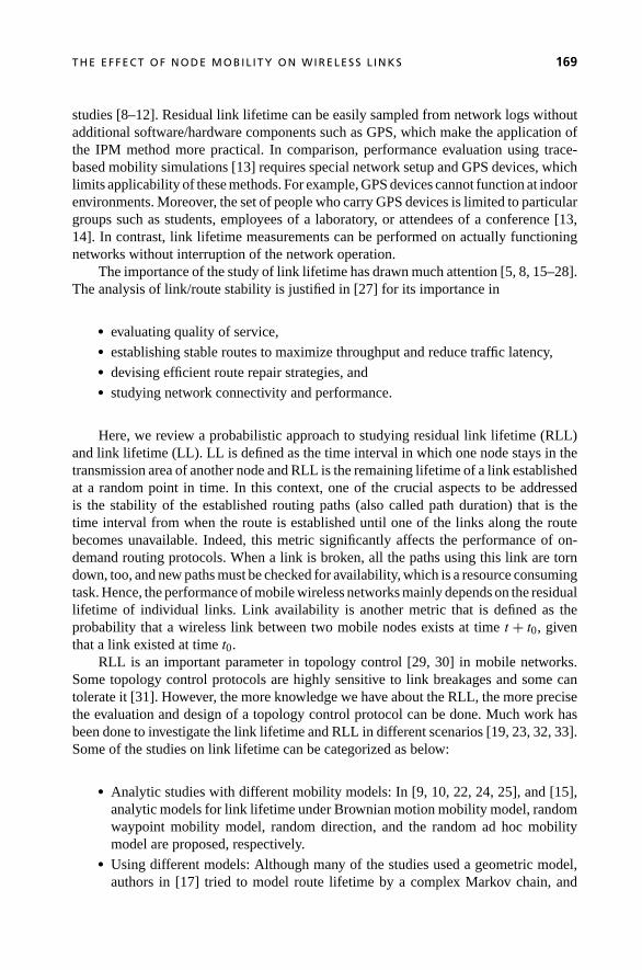
The importance of the study of link lifetime has drawn much attention [5, 8, 15–28].The analysis of link/route stability is justified in [27] for its importance in

• evaluating quality of service,• establishing stable routes to maximize throughput and reduce traffic latency,• devising efficient route repair strategies, and• studying network connectivity and performance.

Here, we review a probabilistic approach to studying residual link lifetime (RLL)and link lifetime (LL). LL is defined as the time interval in which one node stays in thetransmission area of another node and RLL is the remaining lifetime of a link establishedat a random point in time. In this context, one of the crucial aspects to be addressedis the stability of the established routing paths (also called path duration) that is thetime interval from when the route is established until one of the links along the routebecomes unavailable. Indeed, this metric significantly affects the performance of on-demand routing protocols. When a link is broken, all the paths using this link are torndown, too, and new paths must be checked for availability, which is a resource consumingtask. Hence, the performance of mobile wireless networks mainly depends on the residuallifetime of individual links. Link availability is another metric that is defined as theprobability that a wireless link between two mobile nodes exists at time t + t0, giventhat a link existed at time t0.

RLL is an important parameter in topology control [29, 30] in mobile networks.Some topology control protocols are highly sensitive to link breakages and some cantolerate it [31]. However, the more knowledge we have about the RLL, the more precisethe evaluation and design of a topology control protocol can be done. Much work hasbeen done to investigate the link lifetime and RLL in different scenarios [19, 23, 32, 33].Some of the studies on link lifetime can be categorized as below:

• Analytic studies with different mobility models: In [9, 10, 22, 24, 25], and [15],analytic models for link lifetime under Brownian motion mobility model, randomwaypoint mobility model, random direction, and the random ad hoc mobilitymodel are proposed, respectively.

• Using different models: Although many of the studies used a geometric model,authors in [17] tried to model route lifetime by a complex Markov chain, and


authors in [28] provided an approximation model for link lilfetime based on atwo-state Markov chain.

• Pure simulation-based or experimental studies: Link lifetime evaluations in[5, 16, 19] are based only on simulation experiments. An experimental studyof link statistics for a mobile network in a laboratory environment is reported in[26]. Authors in [16] experimentally investigate the link stability.

Here, we will review a geometrical model used to obtain a closed-form expressionfor the residual link lifetime PDF (probability density function). Then, we will studysome aspects of RLL and link lifetime.

8.2.1 Geometric Modeling

Several geometric models are proposed to study RLL or link lifetime [9, 10, 18, 23].However, modeling of RLL or link lifetime is a delicate probabilistic/geometric issue.For example, a small mistake in assumptions in [8] led to large errors in the results, whichis commented on in [34]. Here, we review a sample geometric model for RLL analysis.

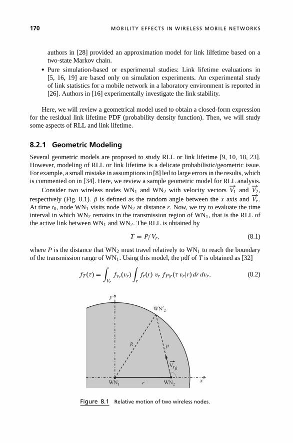
Consider two wireless nodes WN1 and WN2 with velocity vectors−→V1 and

−→V2,

respectively (Fig. 8.1). β is defined as the random angle between the x axis and−→Vr .

At time t0, node WN1 visits node WN2 at distance r. Now, we try to evaluate the timeinterval in which WN2 remains in the transmission region of WN1, that is the RLL ofthe active link between WN1 and WN2. The RLL is obtained by

T = P/Vr, (8.1)

where P is the distance that WN2 must travel relatively to WN1 to reach the boundaryof the transmission range of WN1. Using this model, the pdf of T is obtained as [32]

fT (τ) =∫

Vr

fvr (vr)∫

r

fr(r) vr fP |r(τ vr|r) dr dvr, (8.2)

Figure 8.1 Relative motion of two wireless nodes.

THE EFFECT OF NODE MOBIL ITY ON WIRELESS L INKS 171

where

fr(r) = 2r

R2, 0 ≤ r ≤ R (8.3)

and

fP |r(p|r) = 1

π

R2+p2−r2

p2 r√4 − (R2−p2−r2)2

p2 r2

, R − r ≤ p ≤ R + r. (8.4)

This relation is applicable for centro-symmetric mobility models. Using this relation, thedistribution of RLL is obtained given the distribution of relative velocity. For example,for constant velocity mobility model [23], in which nodes move with a constant velocity(|−→V | = vc) in a random direction, the pdf of relative velocity is obtained [9, 10] as

fVr (vr) = 2

π√

4v2c − v2

r

× [U(vr) − U(vr − 2 vc)], (8.5)

where U is the unit step function. Therefore, the pdf of RLL is obtained as

fT (τ) = 1

π2R2τ[4τvcR + 2(R − τvc)(R + τvc) ln(

R + τvc

|R − τvc| )]. (8.6)

Expression (8.6) can be used as a tight approximation of the distribution of RLL for thetraditional random direction mobility model as well. According to [32], the pdf of linklifetime is obtained by

fD(τ) = −dfT (τ)

dτ× π2R

8 vc

. (8.7)

8.2.2 LL and RLL Properties

Based on the model in [32], it is shown that the expected value of RLL is infinite whilethe average of LL is finite. That is why LL is proposed as a performance or connectivitymetric in the literature [23, 35], while RLL is never used as a metric. Maybe it looks likea paradox that the expected value of whole link lifetime is finite and the expected value ofresidual link lifetime (a portion of link lifetime) is greater. One may think that, becauselink establishment is performed at a random point of time (over the link lifetime) theaverage of the residual link lifetime must be half of the average of total link lifetime andconsequently could not be greater than the average of the link lifetime. However, the caseis analogous to the inspection paradox [36]. Briefly, when a node tries to establish a link,the neighbors with larger LL are more likely to be detected. In other words, average linklifetime is directly affected by the frequency of visiting (entrances to the transmissionrange) different nodes with different velocities, whereas average residual link lifetimeis directly affected by the density of different nodes with different link lifetimes in thevicinity of a particular node [34].


Another interesting outcome of the closed-form expression for the pdf of RLL isthat we can easily show RLL has a long-tailed distribution [33] and thus is heavy-tailedsince every long-tailed distribution is also heavy-tailed [37]. RLL has no finite mean orany higher moment. LL in the case of the constant velocity model has also a long-taileddistribution. However, LL has a finite mean but no higher moments. These results revealimportant facts about the behavior of LL and RLL random variables. Intuitively, thesetwo random variables take small values frequently and very large values rarely. This canbe of help to network designers in avoiding false heuristic assumptions. For example,a network designer may measure the average and variance of RLL from the logs of anactual network and estimate some RLL based on that. However, the results here confirmthat, firstly, the average of RLL is not a stable measure and cannot provide only concretefacts about RLL distribution. Secondly, as RLL takes small values frequently and verylarge values rarely, most of the realistic samples of RLL are not close to the calculatedaverage from the logs.

Other outcomes of the model are the investigation of the effect of the number ofstationary nodes on the LL and RLL, investigation of the effect of buffer zone on the LLand RLL, and study of the behavior of LL and RLL in multivelocity mobility models [33].

In the next section, we will investigate the effect of mobility on network topology.As delivering pure analytic methods for this case are very complicated, we will use somefacts obtained through simulation to ease the study.

8.3 THE EFFECT OF NODE MOBILITY ON NETWORK TOPOLOGY

It is a widely accepted fact that the limited energy available at the nodes of a wirelessmobile network must be used as efficiently as possible [38]. If energy conservationtechniques are used at different levels, the functional lifetime of both individual nodes andthe network can be extended considerably. For this reason, energy conserving protocolsat the MAC, routing, and upper layers have been proposed [39, 40]. Further energycan be saved if the network topology itself is energy-efficient, that is, if transmissionranges of the nodes are set in such a way that a target property (e.g., connectivity) ofthe resulting network topology is guaranteed, while the global energy consumption isreduced. Decreasing the nodes’ transmission power with respect to the maximum levelpotentially has two positive effects: (i) reducing nodes’ energy consumption, and (ii)increasing the spatial reuse, with a positive overall effect on network capacity [41].

Here, we will study a phase transition phenomenon in connectivity of topologiesmade by homogeneous topology control and k-Neigh topology control protocol, andbased on that we find a relation between topology update time and transmission range.

The simplest form of topology control is homogeneous topology control, where afixed value of transmission range is used for all nodes [29]. In the case that mobile nodesdo not have a mechanism to adjust their transmission power adaptively at run time, it isthe only possible solution. Thus, determining a proper global transmission range for thiskind of topology control is of great importance [29, 42–45].

The topology constructed by the TC protocol is called logical topology. Each nodekeeps a list of logical neighbors in the logical topology and only communicates with them.

THE EFFECT OF NODE MOBIL ITY ON NETWORK TOPOLOGY 173

The logical topology is required to be connected. Several protocols could be executed ontop of the logical topology and could construct a subgraph (e.g., a broadcast tree) out ofit. Connectivity of the logical topology is a necessary condition for connectivity of suchstructures. The connectivity is ensured under all localized topology control protocolswhen the network is static. However, due to node mobility, there is no guarantee that alogical neighbor is within the transmission range at a later time. In this case, some logicalneighbors are no longer reachable while others are still reachable (reachable neighborsare called effective neighbors). The union of the effective neighbor sets of all nodes formsan effective topology [31].

In case of homogeneous topology control, all the physical neighbors within criticaltransmission range are listed as logical neighbor list upon receiving a “hello” messagefrom each other. An important problem in application of TC protocols under mobilityconditions is the evaluation and determination of “hello” interval in order to conservemore energy while preserving connectivity. Obviously, setting a small value for “hello”interval leads to frequent execution of TC and more energy consumption. On the otherhand, setting a high value for this important parameter may lead to a disconnectedeffective topology in a portion of the network lifetime unless the transmission rangeof the nodes is increased to keep the network connected, which will increase powerconsumption of the network in another way. Therefore, there is an optimal setting fortransmission range and “hello” interval. To obtain such an optimal point, we need tohave the relation between the transmission range and the “hello” interval that keeps thenetwork connected.

The k-Neigh [46] topology protocol is based on the construction of a logical topologythrough connecting each node to its K nearest neighbors. Unidirectional links are eitherremoved or converted into bidirectional edges. k-Neigh is a simple, fully distributed,asynchronous, and localized protocol that relies only on distance estimation, a techniquethat can be implemented at a reasonable cost in many realistic scenarios, and it does notneed location information or angle of arrival (AoA) data to construct the topology.

In order to study mobility tolerance of a topology, we need to first define the connec-tivity requirement as a quantitative metric. In the next section, we will provide a formaldefinition of connectivity for the sake of this study.

8.3.1 Definitions of Connectivity

Below, some of the connectivity terms introduced in the literature are reviewed.

• Strict connectivity (SCON): Strict connectivity [31] is defined as traditional math-ematical connectivity.

• Weak connectivity (WCON): There are different definitions for the weak con-nectivity. In several cases, the main goal behind defining a weak connectivitycondition is for practical considerations. The rationale is that the network de-signer could be interested in maintaining only a certain fraction of the nodesconnected, if this would result in significant energy savings. In [31], the weakconnectivity is defined in terms of capability of completing a connectivity related


task, such as global flooding, measured in terms of the percentage of nodes thatreceive the message. In [46], a network is called weakly connected when at least95% of network nodes belong to the same connected component with probabilityof at least 0.95.

In [12], the following statistical connectivity requirements are defined:

• Statistical strict connectivity, SSC(α), is satisfied if the network is strongly con-nected with probability at least α.

• Mean largest connected component ratio, MLCCR (α), is satisfied if MLCCR≥ α where MLCCR is the ratio of the mean size of the largest connected compo-nent to the size of whole network and α is a parameter over [0,1] (size of a networkor a component is defined as the number of nodes included in it). For example, arandom graph satisfies MLCCR(0.95) if the average of largest connected compo-nent covers at least 95% of the nodes. In practice, we can measure MLCCR on alarge set of topologies.

• Weak connectivity probability, WCP (α, β), is satisfied if WCP ≥α where WCPis the probability of observing a weakly connected network and α and β areparameters over [0,1]. A network is considered weakly connected if the ratio ofthe size of the largest connected component to the size of network is greater thanor equal to β. For example, a random graph satisfies WCP(0.8,0.95) if the largestconnected component covers at least 95% of nodes with probability of 0.8 orhigher. Obviously, WCP(α, 1) is equivalent to SSC(α).

Now, we can formalize the problem of determining “hello” interval as the evaluationof statistical topology lifetime.

• Statistical topology lifetime (STL): Statistical topology lifetime is the maximumtime interval after construction of the topology in which a specific statisticalconnectivity requirement is met.

8.3.2 Phase Transition Phenomenon in Connectivity andDisconnection Degree

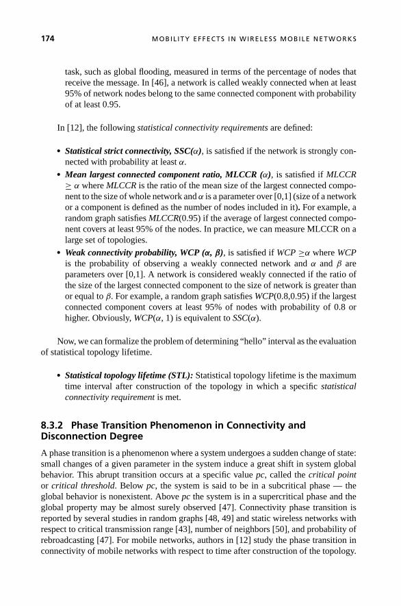
A phase transition is a phenomenon where a system undergoes a sudden change of state:small changes of a given parameter in the system induce a great shift in system globalbehavior. This abrupt transition occurs at a specific value pc, called the critical pointor critical threshold. Below pc, the system is said to be in a subcritical phase — theglobal behavior is nonexistent. Above pc the system is in a supercritical phase and theglobal property may be almost surely observed [47]. Connectivity phase transition isreported by several studies in random graphs [48, 49] and static wireless networks withrespect to critical transmission range [43], number of neighbors [50], and probability ofrebroadcasting [47]. For mobile networks, authors in [12] study the phase transition inconnectivity of mobile networks with respect to time after construction of the topology.

THE EFFECT OF NODE MOBIL ITY ON NETWORK TOPOLOGY 175

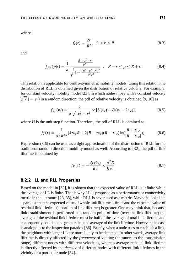
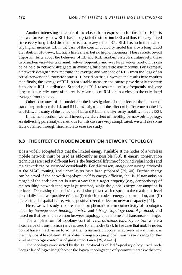
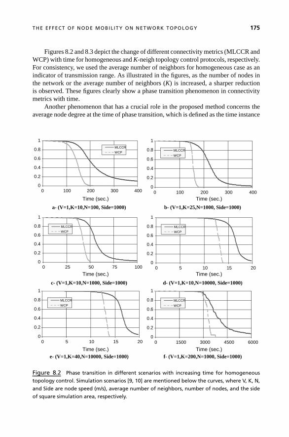
Figures 8.2 and 8.3 depict the change of different connectivity metrics (MLCCR andWCP) with time for homogeneous and K-neigh topology control protocols, respectively.For consistency, we used the average number of neighbors for homogeneous case as anindicator of transmission range. As illustrated in the figures, as the number of nodes inthe network or the average number of neighbors (K) is increased, a sharper reductionis observed. These figures clearly show a phase transition phenomenon in connectivitymetrics with time.

Another phenomenon that has a crucial role in the proposed method concerns theaverage node degree at the time of phase transition, which is defined as the time instance

0

0.2

0.4

0.6

0.8

1

4003002001000

MLCCR

WCP

Time (sec.)

0

0.2

0.4

0.6

0.8

1

4003002001000

MLCCR

WCP

Time (sec.)

Time (sec.) Time (sec.)


a- (V=1,K=10,N=100, Side=1000) b- (V=1,K=25,N=1000, Side=1000)

0

0.2

0.4

0.6

0.8

1

1007550250

MLCCR

WCP

0

0.2

0.4

0.6

0.8

1

20151050

MLCCR

WCP

c- (V=1,K=10,N=1000, Side=1000) d- (V=1,K=10,N=10000, Side=1000)

0

0.2

0.4

0.6

0.8

1

20151050

MLCCR

WCP

0

0.2

0.4

0.6

0.8

1

60004500300015000

MLCCR

WCP

e- (V=1,K=40,N=10000, Side=1000) f- (V=1,K=200,N=1000, Side=1000)

Figure 8.2 Phase transition in different scenarios with increasing time for homogeneous

topology control. Simulation scenarios [9, 10] are mentioned below the curves, where V, K, N,

and Side are node speed (m/s), average number of neighbors, number of nodes, and the side

of square simulation area, respectively.


0

0.2

0.4

0.6

0.8

1

4003002001000

MLCCR

WCP(0.95)

Time (sec.)

0

0.2

0.4

0.6

0.8

1

4003002001000

MLCCR

WCP(0.95)

Time (sec.)



a- (V=1,K=10,N=100, Side=1000) b- (V=1,K=25,N=1000, Side=1000)

0

0.2

0.4

0.6

0.8

1

604530150

MLCCR

WCP(0.95)

0

0.2

0.4

0.6

0.8

1

20151050

MLCCR

WCP(0.95)

c- (V=1,K=10,N=1000, Side=1000) d- (V=1,K=10,N=10000, Side=1000)

0

0.2

0.4

0.6

0.8

1

20151050

MLCCR

WCP(0.95)

0

0.2

0.4

0.6

0.8

1

60004500300015000

MLCCR

WCP(0.95)

e- (V=1,K=40,N=10000, Side=1000) f- (V=1,K=200,N=1000, Side=1000)

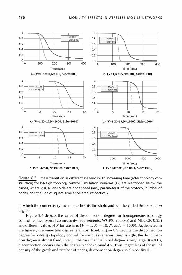
Figure 8.3 Phase transition in different scenarios with increasing time (after topology con-

struction) for k-Neigh topology control. Simulation scenarios [12] are mentioned below the

curves, where V, K, N, and Side are node speed (m/s), parameter K of the protocol, number of

nodes, and the side of square simulation area, respectively.

in which the connectivity metric reaches its threshold and will be called disconnectiondegree.

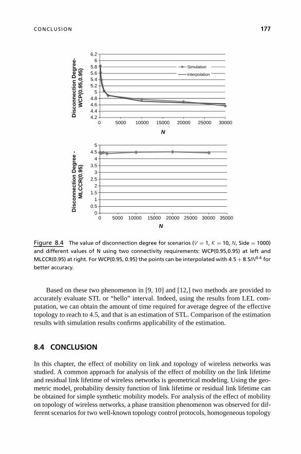
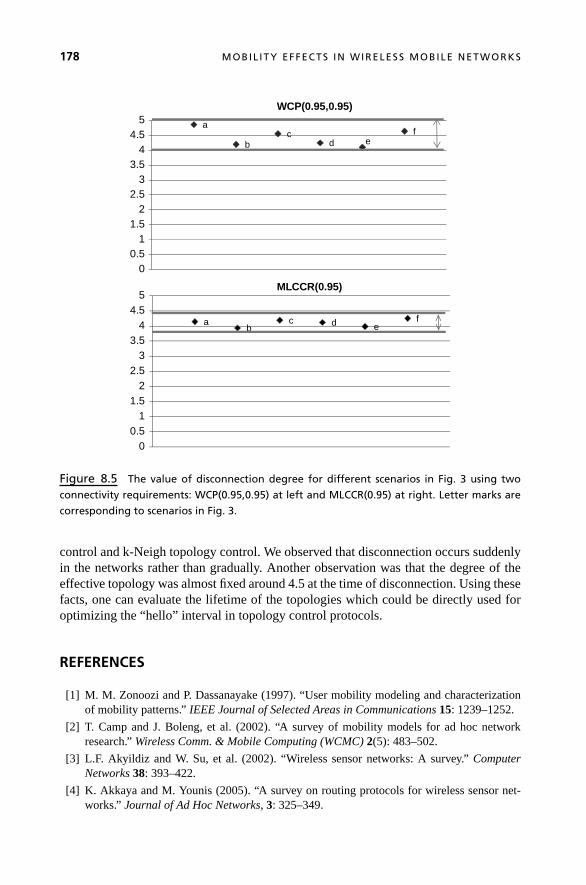
Figure 8.4 depicts the value of disconnection degree for homogeneous topologycontrol for two typical connectivity requirements: WCP(0.95,0.95) and MLCCR(0.95)and different values of N for scenario (V = 1, K = 10, N, Side = 1000). As depicted inthe figures, disconnection degree is almost fixed. Figure 8.5 depicts the disconnectiondegree for k-Neigh topology control for various scenarios. Surprisingly, the disconnec-tion degree is almost fixed. Even in the case that the initial degree is very large (K=200),disconnection occurs when the degree reaches around 4.5. Thus, regardless of the initialdensity of the graph and number of nodes, disconnection degree is almost fixed.

CONCLUS ION 177

4.24.44.64.8

55.25.45.65.8

66.2

300002500020000150001000050000

Dis

con

nec

tio

n D

egre

e-W

CP

(0.9

5,0.

95)

N

Simulation

Interpolation

00.5

11.5

22.5

33.5

44.5

5

35000300002500020000150001000050000

Dis

con

nec

tio

n D

egre

e -

ML

CC

R(0

.95)

N

Figure 8.4 The value of disconnection degree for scenarios (V = 1, K = 10, N, Side = 1000)

and different values of N using two connectivity requirements: WCP(0.95,0.95) at left and

MLCCR(0.95) at right. For WCP(0.95, 0.95) the points can be interpolated with 4.5 + 8.5/N0.4 for

better accuracy.

Based on these two phenomenon in [9, 10] and [12,] two methods are provided toaccurately evaluate STL or “hello” interval. Indeed, using the results from LEL com-putation, we can obtain the amount of time required for average degree of the effectivetopology to reach to 4.5, and that is an estimation of STL. Comparison of the estimationresults with simulation results confirms applicability of the estimation.

8.4 CONCLUSION

In this chapter, the effect of mobility on link and topology of wireless networks wasstudied. A common approach for analysis of the effect of mobility on the link lifetimeand residual link lifetime of wireless networks is geometrical modeling. Using the geo-metric model, probability density function of link lifetime or residual link lifetime canbe obtained for simple synthetic mobility models. For analysis of the effect of mobilityon topology of wireless networks, a phase transition phenomenon was observed for dif-ferent scenarios for two well-known topology control protocols, homogeneous topology


a

bc

d ef

00.5

11.5

22.5

33.5

44.5

5WCP(0.95,0.95)

ab

c d ef

00.5

11.5

22.5

33.5

44.5

5MLCCR(0.95)

Figure 8.5 The value of disconnection degree for different scenarios in Fig. 3 using two

connectivity requirements: WCP(0.95,0.95) at left and MLCCR(0.95) at right. Letter marks are

corresponding to scenarios in Fig. 3.

control and k-Neigh topology control. We observed that disconnection occurs suddenlyin the networks rather than gradually. Another observation was that the degree of theeffective topology was almost fixed around 4.5 at the time of disconnection. Using thesefacts, one can evaluate the lifetime of the topologies which could be directly used foroptimizing the “hello” interval in topology control protocols.

REFERENCES

[1] M. M. Zonoozi and P. Dassanayake (1997). “User mobility modeling and characterizationof mobility patterns.” IEEE Journal of Selected Areas in Communications 15: 1239–1252.

[2] T. Camp and J. Boleng, et al. (2002). “A survey of mobility models for ad hoc networkresearch.” Wireless Comm. & Mobile Computing (WCMC) 2(5): 483–502.

[3] L.F. Akyildiz and W. Su, et al. (2002). “Wireless sensor networks: A survey.” ComputerNetworks 38: 393–422.

[4] K. Akkaya and M. Younis (2005). “A survey on routing protocols for wireless sensor net-works.” Journal of Ad Hoc Networks, 3: 325–349.

REFERENCES 179

[5] N. Sadagopan and F. Bai, et al. (2003). PATHS: Analysis of Path Duration Statistics and theImpact on Reactive MANET Routing Protocols. ACM MobiHoc, Annapolis (MD).

[6] G. Cao and G. Kesidis, et al. (2005). “Purposeful mobility in tactical sensor networks.” SensorNetwork Operations, IEEE Press, Piscataway, NJ, pp. 113–126.

[7] D. Johnson and T. Stack, et al. (2006). “TrueMobile: A Mobile Robotic Wireless and SensorNetwork Testbed.” INFOCOMM.

[8] P. Samar and S. B. Wicker (2006). “Link dynamics and protocol design in a multihop mobileenvironment.” IEEE Transactions on Mobile Computing 5(9).

[9] A. Nayebi and H. Sarbazi-Azad (2007a). “Lifetime analysis of the logical topology con-structed by homogeneous topology control in wireless mobile networks.” The 13th Interna-tional Conference on Parallel and Distributed Systems (ICPADS), Taiwan, IEEE Publishing.

[10] A. Nayebi and H. Sarbazi-Azad (2007b). “A model for link excess life in mobile wirelessnetworks.” Technical report 2007-118, HPCAN lab., Sharif University of Technology, Tehran,Iran.

[11] A. Nayebi and G. Karlsson (2008). Neighbor Discovery in Mobile Wireless Networks. Stock-holm, Sweden, Royal Institute of Technology (KTH), Technical report: TRITA-EE 2008:066.

[12] A. Nayebi and H. Sarbazi-Azad (2009). “Analysis of k-Neigh topology control protocol formobile wireless networks.” Computer Networks 53(5): 613–633.

[13] I. Rhee and M. Shin, et al. (2007). “Human mobility patterns and their impact on routing inhuman-driven mobile networks.” Sixth Workshop on Hot Topics in Networks (HotNets-VI).

[14] P. Hui and A. Chaintreau, et al. (2005). “Pocket switched networks and human mobilityin conference environments.” ACM SIGCOMM Workshop on Delay-Tolerant Networking(WDTN ’05), Philadelphia, PA.

[15] A. B. McDonald and T. Znati (1999). “A path availability model for wireless ad hoc networks.”IEEE WCNC.

[16] M. Gerharz and C. de Waal, et al. (2002). “Link stability in mobile wireless ad hoc networks.”IEEE LCN.

[17] Y.-C. Tseng, Y.-F. Li, et al. (2003). “On route lifetime in multihop mobile ad hoc networks.”IEEE Transactions on Mobile Computing 2(4).

[18] D. Yu and H. Li, et al. (2003). “Path availability in ad-hoc network.” Int’l Conf. on Telecomm.(ICT 2003), Tahiti, France.

[19] F. Bai, and N. Sadagopan, et al. (2004). “Modeling path duration distributions in MANETsand their impact on reactive routing protocols.” IEEE Journal on Selected Areas of Commu-nications (JSAC) 22(7).

[20] Z. Cheng and W. B. Heinzelman (2004). “Exploring long lifetime routing (LLR) in ad hocnetworks.” 7th ACM International Symposium on Modeling, Analysis and Simulation ofWireless and Mobile Systems (MSWIM 2004).

[21] P. Samar and S. B. Wicker (2004). “On the behavior of communication links of a nodein a multi-hop mobile environment.” 5th ACM international symposium on Mobile ad hocnetworking and computing (MobiHoc), Roppongi, Japan.

[22] G. Carofiglio and C. Chiasserini, et al. (2005). Analysis of Route Stability in MANETs. SecondEuroNGI Workshop on New Trends in Modelling, Quantitative Methods and Measurements,Aveiro, Portugal.

[23] S. Cho and J. P. Hayes (2005). “Impact of mobility on connection stability in ad hoc networks.”IEEE WCNC.


[24] Y. Han and R. J. La (2006). “Maximizing path durations in mobile adhoc networks.” 40thAnnual Conference on Information Sciences and Systems, Princeton, NJ.

[25] Y. Han and R. J. La, et al. (2006). “Distribution of path durations in mobile ad-hoc networks—Palm’s Theorem to the rescue.” Computer Networks 50(12): 1887–1900.

[26] V. Lenders and J. Wagner, et al. (2006). Analyzing the Impact of Mobility in Ad HocNetworks. REALMAN06, Florence, Italy.

[27] G. Carofiglio and C. Chiasserini, et al. (2009). “Route stability in MANETs under the randomdirection mobility model.” IEEE Transactions on Mobile Computing 8(9): 1167–1179.

[28] X. Wu and H. R. Sadjadpour, et al. (2009). “From link dynamics to path lifetime and packet-length optimization in MANETs. Computer Networks 15(5): 637–650.

[29] P. Santi (2005). “The critical transmitting range for connectivity in mobile ad hoc networks.”IEEE Transactions on Mobile Computing 4(3).

[30] P. Santi (2005). Topology Control in Wireless Ad Hoc and Sensor Networks, John Wiley andSons.

[31] J. Wu and F. Dai (2006). “Mobility-sensitive topology control in mobile ad hoc networks.”IEEE Transactions on Parallel and Distributed Systems 17(6).

[32] A. Nayebi and A. Khosravi, et al. (2007). “On the link excess life in mobile wireless networks.”International Conference on Computing: Theory and Applications ICCTA, IEEE ComputerSociety.

[33] A. Nayebi and H. Sarbazi-Azad (2012). “Analysis of link lifetime in wireless mobile net-works.” Ad Hoc Networks 10(7): 1221–1237.

[34] A. Nayebi (2011). “A comment on link dynamics and protocol design in a multi-hop mobileenvironment.” Wireless Sensor Network 3(3): 114–116.

[35] F. Bai, and N. Sadagopan, et al. (2003). “The IMPORTANT framework for analyzing theimpact of mobility on performance of routing for ad hoc networks.” Ad Hoc Networks 1(4):383–403.

[36] S. M. Ross (1985). Introduction to Probability Models, Academic Press.

[37] S. Asmussen (2003). Applied Probability and Queues. Berlin, Springer.

[38] M. Ilyas and I. Mahgoub (2004). Handbook of Sensor Networks: Compact Wireless andWired Sensing Systems, CRC Press.

[39] L. Demirkol and C. Ersoy, et al. (2006). “MAC protocols for wireless sensor networks: asurvey.” IEEE Communications Magazine 44(4): 115–121.

[40] J. Ben-Othman and B. Yahya (2010). “Energy efficient and QoS based routing proto-col for wireless sensor networks.” Journal of Parallel and Distributed Computing 70(8):849–857.

[41] V. Kawadia and P. R. Kumar (2003). “Power control and clustering in ad hoc networks.”IEEE INFOCOM 03.

[42] M. D. Penrose (1997). “The longest edge of the random minimal spanning tree.” The Annalsof Applied Probability 7(2): 340–361.

[43] P. Gupta and P. R. Kumar (1998). “Critical power for asymptotic connectivity.” 37th IEEEConference on Decision and Control.

[44] P. Santi and D. M. Blogh (2002). “An evaluation of connectivity in mobile wireless ad hocnetworks.” International Conference on Dependable Systems and Networks (DSN’02).

[45] P. Santi and D. Blough (2003). “The critical transmitting range for connectivity in sparsewireless ad hoc networks.” IEEE Transactions on Mobile Computing 2(1): 25–39.

REFERENCES 181

[46] D. M. Blough and M. Leoncini, et al. (2006). “The k-Neighbors Approach to InterferenceBounded and Symmetric Topology Control in Ad Hoc Networks.” IEEE Transactions onMobile Computing 5.

[47] Y. Sasson and D. Cavin, et al. (2002). Probabilistic Broadcast for Flooding in Wireless MobileAd hoc Networks Swiss Federal Institute of Technology (EPFL).

[48] P. Erdos and A. Renyi (1960). “On the evolution of random graphs.” Publications of theMathematical Institute of the Hungarian Academy of Sciences 5: 17–61.

[49] B. Bollobas (1985). Random Graphs. New York, Academic Press.

[50] U. N. Raghavan and H. P. Thadakamalla, et al. (2005). “Phase transitions and connectiv-ity in distributed wireless sensors networks.” 13th International Conference on AdvancedComputing & Communications.

Documents

Large Scale Network-Centric Distributed Systems || Mobility Effects In Wireless Mobile Networks