Large scale simulation of particlecoating using coupled CFD-DEMMaster’s thesis in Applied Mechanics

ANAND HARIHARAN

Department of Mechanics and Maritime SciencesCHALMERS UNIVERSITY OF TECHNOLOGYGöteborg, Sweden 2020

MASTER’S THESIS IN APPLIED MECHANICS

Large scale simulation of particle coating using coupled CFD-DEM

ANAND HARIHARAN

Department of Mechanics and Maritime Sciences

Division of Fluid Dynamics

CHALMERS UNIVERSITY OF TECHNOLOGY

Göteborg, Sweden 2020

Large scale simulation of particle coating using coupled CFD-DEMANAND HARIHARAN

c© ANAND HARIHARAN, 2020

Master’s thesis 2020:75Department of Mechanics and Maritime SciencesDivision of Fluid DynamicsChalmers University of TechnologySE-412 96 GöteborgSwedenTelephone: +46 (0)31-772 1000

Chalmers ReproserviceGöteborg, Sweden 2020

Large scale simulation of particle coating using coupled CFD-DEMMaster’s thesis in Applied MechanicsANAND HARIHARANDepartment of Mechanics and Maritime SciencesDivision of Fluid DynamicsChalmers University of Technology

AbstractSpouted fluidized beds are widely used for particle coating because of its excellent mixing rates andfavorable heat and mass transfer characteristics. The combination of Computational Fluid Dynamics(CFD) and the Discrete Element Method (DEM) has previously been employed for simulation ofthe complex phenomena of such processes. However, simulating a fluidized bed on a large scalewith DEM requires exceptional computational power as all the interactions between the particlesare fully resolved. In addition, simulating the spray droplets further increases the computationaldemand. Accordingly, coupled DEM and CFD simulations with a well resolved spray have typicallybeen limited to system sizes from a few thousand up to much less than a million particles.

The goal of the current thesis was to perform spray coating simulations on systems with more than 1million particles, including a Lagrangian spray phase and a well resolved fluid. The thesis is carriedout using the DEM-CFD solver IPS FluidizationTM developed at Fraunhofer Chalmers Centre. Thesolver is based on an in-house DEM code and the in-house immersed boundary CFD code IBOFlow R©.Due to heavy use of the Graphical Processing Unit (GPU), the code allows simulating a large numberof particles and a well resolved fluid on a standard desktop computer.

In the first part of the thesis, single spout simulations are carried out to validate the coupled solver.The simulations show excellent agreement with the experimental data available in the open literature.Further, 1D studies are conducted for verifying the heat transfer model. The numerical predictions areshown to be accurate based on comparisons with analytical 1D models. Finally, large scale simulationsincluding the spray and drying are conducted on a Wurster bed system with both the particles andthe spray considered in a Lagrangian sense. The simulations show the versatility of the tool and thepossibility to e.g. characterize the particle coating thickness in terms of the original particle size, aswell as it proves applicability to cases with more than 1 million particles.

Keywords: CFD, DEM, particle coating, Wurster bed, fluidization, GPU

i

AcknowledgementsI would like to express my immense gratitude for my supervisor and my mentor Klas Jareteg whoguided me throughout my Master’s program until my thesis. I am extremely grateful for the immenseknowledge I had gained from him from the interesting discussions. Without his continuous guidanceand persistent help my thesis would not have been possible.I would like to extend my gratitude for Franziska Hunger for guiding me in conducting varioussimulations in my Master’s thesis.I would also like to thank Fredrik Edelvik (Head of department) at Fraunhofer-Chalmers Centre(FCC) for extending me an opportunity to work as a contracted student until my thesis at FCC. Iwould also like to thank FCC for providing me with required computational resources while pursuingmy thesis.

I extend my gratitude for my examiner Srdjan Sasic for his valuable feedbacks and guidance duringthe course of this thesis.

Finally, I would like to thank my family and friends, who have been my constant source of motivationand support during my master’s journey.

ii

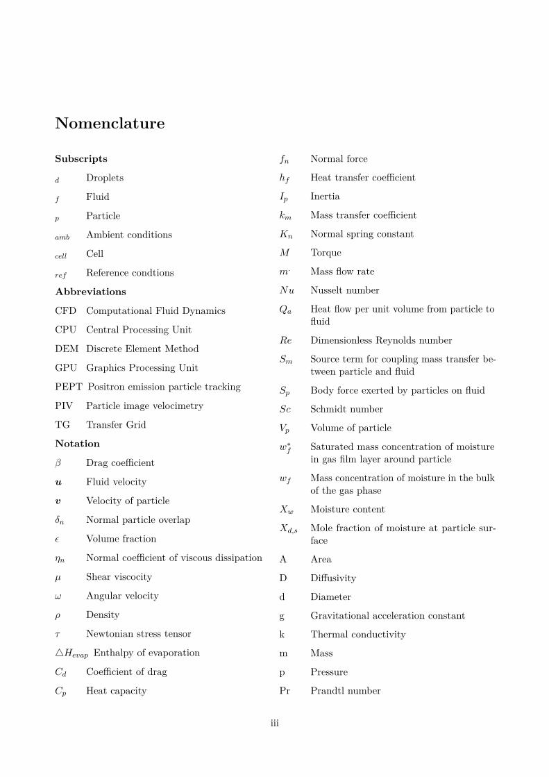
Nomenclature

Subscripts

d Droplets

f Fluid

p Particle

amb Ambient conditions

cell Cell

ref Reference condtions

Abbreviations

CFD Computational Fluid Dynamics

CPU Central Processing Unit

DEM Discrete Element Method

GPU Graphics Processing Unit

PEPT Positron emission particle tracking

PIV Particle image velocimetry

TG Transfer Grid

Notation

β Drag coefficient

u Fluid velocity

v Velocity of particle

δn Normal particle overlap

ε Volume fraction

ηn Normal coefficient of viscous dissipation

µ Shear viscocity

ω Angular velocity

ρ Density

τ Newtonian stress tensor

4Hevap Enthalpy of evaporation

Cd Coefficient of drag

Cp Heat capacity

fn Normal force

hf Heat transfer coefficient

Ip Inertia

km Mass transfer coefficient

Kn Normal spring constant

M Torque

m. Mass flow rate

Nu Nusselt number

Qa Heat flow per unit volume from particle tofluid

Re Dimensionless Reynolds number

Sm Source term for coupling mass transfer be-tween particle and fluid

Sp Body force exerted by particles on fluid

Sc Schmidt number

Vp Volume of particle

w∗f Saturated mass concentration of moisturein gas film layer around particle

wf Mass concentration of moisture in the bulkof the gas phase

Xw Moisture content

Xd,s Mole fraction of moisture at particle sur-face

A Area

D Diffusivity

d Diameter

g Gravitational acceleration constant

k Thermal conductivity

m Mass

p Pressure

Pr Prandtl number

iii

iv

Contents

Abstract i

Acknowledgements ii

Contents v

1 Introduction 21.1 Physics of fluidized beds . . . . . . . . . . . . . . . . . . . . . . . . . . . . . . . . . . . . . 21.2 Physics of spouted fluidized beds . . . . . . . . . . . . . . . . . . . . . . . . . . . . . . . . 21.3 Modeling of spouted fluidized beds . . . . . . . . . . . . . . . . . . . . . . . . . . . . . . . 31.4 Purpose of the project . . . . . . . . . . . . . . . . . . . . . . . . . . . . . . . . . . . . . . 51.5 Simulation software . . . . . . . . . . . . . . . . . . . . . . . . . . . . . . . . . . . . . . . 51.6 Experimental Data . . . . . . . . . . . . . . . . . . . . . . . . . . . . . . . . . . . . . . . . 61.7 Structure of the thesis . . . . . . . . . . . . . . . . . . . . . . . . . . . . . . . . . . . . . . 7

2 Theory 82.1 Computational Fluid Dynamics . . . . . . . . . . . . . . . . . . . . . . . . . . . . . . . . . 82.1.1 Mass and momentum conservation . . . . . . . . . . . . . . . . . . . . . . . . . . . . . . 82.1.2 Heat transfer . . . . . . . . . . . . . . . . . . . . . . . . . . . . . . . . . . . . . . . . . . 92.1.3 Moisture conservation equation . . . . . . . . . . . . . . . . . . . . . . . . . . . . . . . . 92.2 Discrete Element Method . . . . . . . . . . . . . . . . . . . . . . . . . . . . . . . . . . . . 92.2.1 Particle Governing Equation . . . . . . . . . . . . . . . . . . . . . . . . . . . . . . . . . 102.2.2 Heat transfer Model . . . . . . . . . . . . . . . . . . . . . . . . . . . . . . . . . . . . . . 122.2.3 Mass transfer model . . . . . . . . . . . . . . . . . . . . . . . . . . . . . . . . . . . . . . 132.3 Spray droplets . . . . . . . . . . . . . . . . . . . . . . . . . . . . . . . . . . . . . . . . . . 142.4 Multiphase Coupling . . . . . . . . . . . . . . . . . . . . . . . . . . . . . . . . . . . . . . . 142.4.1 Momentum Exchange . . . . . . . . . . . . . . . . . . . . . . . . . . . . . . . . . . . . . 152.4.2 Energy exchange between the phases . . . . . . . . . . . . . . . . . . . . . . . . . . . . . 172.4.3 Mass exchange between the phases . . . . . . . . . . . . . . . . . . . . . . . . . . . . . . 18

3 Methodology 193.1 CFD solution procedure . . . . . . . . . . . . . . . . . . . . . . . . . . . . . . . . . . . . . 193.2 DEM algorithm . . . . . . . . . . . . . . . . . . . . . . . . . . . . . . . . . . . . . . . . . . 193.3 Coupling method . . . . . . . . . . . . . . . . . . . . . . . . . . . . . . . . . . . . . . . . . 203.3.1 Data transfer . . . . . . . . . . . . . . . . . . . . . . . . . . . . . . . . . . . . . . . . . . 213.3.2 Coupling scheme . . . . . . . . . . . . . . . . . . . . . . . . . . . . . . . . . . . . . . . . 22

4 Simulation cases 244.1 Single Spout Bed simulation . . . . . . . . . . . . . . . . . . . . . . . . . . . . . . . . . . . 244.1.1 Geometry of the single spout bed . . . . . . . . . . . . . . . . . . . . . . . . . . . . . . . 244.1.2 Mesh and boundary conditions . . . . . . . . . . . . . . . . . . . . . . . . . . . . . . . . 244.1.3 Physics Modelling and result extraction . . . . . . . . . . . . . . . . . . . . . . . . . . . 264.2 Heat transfer Simulation . . . . . . . . . . . . . . . . . . . . . . . . . . . . . . . . . . . . . 274.2.1 Numerical settings used for heat transfer model verification . . . . . . . . . . . . . . . . 274.3 Spray Simulations . . . . . . . . . . . . . . . . . . . . . . . . . . . . . . . . . . . . . . . . 274.3.1 Geometry of the Wurster Bed . . . . . . . . . . . . . . . . . . . . . . . . . . . . . . . . . 274.3.2 Mesh and Boundary conditions . . . . . . . . . . . . . . . . . . . . . . . . . . . . . . . . 294.3.3 Physics Modelling and result extraction . . . . . . . . . . . . . . . . . . . . . . . . . . . 30

v

5 Results and Discussion 325.1 Single spout bed simulations . . . . . . . . . . . . . . . . . . . . . . . . . . . . . . . . . . 325.1.1 Effect of fluid time step . . . . . . . . . . . . . . . . . . . . . . . . . . . . . . . . . . . . 325.1.2 Momentum-Models . . . . . . . . . . . . . . . . . . . . . . . . . . . . . . . . . . . . . . . 335.1.3 Effect of rolling friction . . . . . . . . . . . . . . . . . . . . . . . . . . . . . . . . . . . . 355.1.4 Effect of friction . . . . . . . . . . . . . . . . . . . . . . . . . . . . . . . . . . . . . . . . 355.2 1D heat transfer simulations . . . . . . . . . . . . . . . . . . . . . . . . . . . . . . . . . . . 365.3 Spray simulations . . . . . . . . . . . . . . . . . . . . . . . . . . . . . . . . . . . . . . . . . 375.3.1 Wurster bed simulations . . . . . . . . . . . . . . . . . . . . . . . . . . . . . . . . . . . . 375.3.2 Wurster bed spray simulations . . . . . . . . . . . . . . . . . . . . . . . . . . . . . . . . 385.3.3 Correlation between particle radius and thickness of the film . . . . . . . . . . . . . . . 38

6 Conclusion 41

References 42

vi

List of Figures

1.1 Schematic of the Wurster bed coating process along with different zones of interest. . . 41.2 Overview of the simulation software, IPS FluidizationTM, including the constituent

parts: IPS IBOFlow c©. . . . . . . . . . . . . . . . . . . . . . . . . . . . . . . . . . . . . 62.1 DEM iteration on a particle: (a) Identification of contacts, (b) Application of force on

the particle, (c) Calculation of net reaction force, and (d) Particle displacement. . . . 102.2 DEM particle-collision Model . . . . . . . . . . . . . . . . . . . . . . . . . . . . . . . . 112.3 Spray process from a spray cone injector, with R as the radius and A as the cone angle. 152.4 Different coupling mechanism: (a): Only fluid field affects the particles (b): Fluid

filed affects the particles and vice-versa (c): Particle-Particle, Particle-Fluid andFluid-Particle interaction. . . . . . . . . . . . . . . . . . . . . . . . . . . . . . . . . . . 16

3.1 Flowchart of the DEM Algorithm. . . . . . . . . . . . . . . . . . . . . . . . . . . . . . 203.2 Different Particle arrangements as available in the IPS Fludization. . . . . . . . . . . . 203.3 A schematic representing the data transfer mechanism between the fluid solver (CPU)

and the DEM solver (GPU). . . . . . . . . . . . . . . . . . . . . . . . . . . . . . . . . . 223.4 Volume fraction calculation in split method . . . . . . . . . . . . . . . . . . . . . . . . 233.5 Flowchart describing the coupling Algorithm used in IPS FluidizationTM. . . . . . . . 234.1 Schematic of Single Spout bed. . . . . . . . . . . . . . . . . . . . . . . . . . . . . . . . 254.2 Line probes location . . . . . . . . . . . . . . . . . . . . . . . . . . . . . . . . . . . . . 264.3 Schematic of the Wursted bed geometry representing different boundary regions. . . . 284.4 Sectional view of the Wurster bed along with the dimension. . . . . . . . . . . . . . . 305.2 Comparison of Momentum transfer coefficients . . . . . . . . . . . . . . . . . . . . . . 335.3 Time averaged particle velocity for different momentum exchange models. . . . . . . . 345.4 Vector plot of time averaged particle axial velocity plots for three different momentum-

exchange models at the end of the simulation (4 sec). . . . . . . . . . . . . . . . . . . . 355.5 Time averaged particle velocity for different values of rolling friction . . . . . . . . . . 365.6 Time averaged particle velocity for different friction-coefficient . . . . . . . . . . . . . 365.7 Comparison of time evolution of temperature between the 1D simulation and IPSFlu-

idization. . . . . . . . . . . . . . . . . . . . . . . . . . . . . . . . . . . . . . . . . . . . 375.8 Comparison of time evolution of temperature for different fluid time steps. . . . . . . . 375.9 Comparison of axial velocity from simulation with the experimental study of Li Liang

et al. . . . . . . . . . . . . . . . . . . . . . . . . . . . . . . . . . . . . . . . . . . . . . . 385.11 Spray accumulation over time with varying flow rates . . . . . . . . . . . . . . . . . . 405.12 Plot showing correlation between the radii of the particle and the spray accumulated

for Nozzle Flow rate = 4.2m3/hr . . . . . . . . . . . . . . . . . . . . . . . . . . . . . . 40

List of Tables

4.1 Dimensions of the single spouted bed used in the simulations. . . . . . . . . . . . . . . 244.2 Particle settings used in the simulations. . . . . . . . . . . . . . . . . . . . . . . . . . . 254.3 Properties used in calculation of momentum transfer co-efficient for the verification study. 274.4 Wursted bed Dimensions . . . . . . . . . . . . . . . . . . . . . . . . . . . . . . . . . . . 294.5 Particle settings used in the Wurster simulations. . . . . . . . . . . . . . . . . . . . . . 314.6 Moisture Properties used in the spray simulations. . . . . . . . . . . . . . . . . . . . . 31

1

1 Introduction

1.1 Physics of fluidized beds

Fluidization is a process in which the granular material is converted from a static solid-like stateto a dynamic fluid-like state. This process occurs when a fluid (liquid or gas) is passed up throughthe granular material from the bottom of the bed. At low velocities, the aerodynamic drag of theparticles is lower than the gravitational force, thus the bed remains in a fixed state. However, furtherincreasing the velocity, increases the drag force on the particle causing the bed to expand in volume,making the particles to move away from each other. At a certain velocity, the aerodynamic force onthe particles is balanced by the gravitational force causing the particles to become suspended withinthe fluid. At this point, the bed is said to be fluidized and it will exhibit fluidic behavior.

The devices using the property of fluidization are typically called fluidized beds. These beds possessexcellent properties, such as a high surface area of contact between the fluid phase and solid particlesper unit bed volume, high levels of intermixing of the particulate phase and frequent particle-particleand particle-wall collisions. This results in enhanced heat and mass transfer rates, high mixingrates and uniform reaction conditions. Hence, such devices have often been applied for processingapplications such as coating, granulation, and drying. The application of fluidized beds, however, hasbeen limited to relatively fine solids. This is because coarse materials when subjected to fluidizationshow a marked tendency toward slugging [1].

1.2 Physics of spouted fluidized beds

In order to overcome the limitation of fluidized beds, spouted beds were developed [2]. Such a bedcomprises of a central nozzle with a high velocity jet, which results in a high velocity region in thecentral portion of the bed and a region with section of particles along the walls. As a result, theparticles in the spout region move in a well structured manner in the vertical direction (with littleradial displacement) accompanied by void (air bubble) propagation [3]. Mathur and Gishler [2] fromtheir experimental studies found that the spout generation in the bed occurs only in a narrow range ofgas flow rates. Nagarkatti and Chatterjee [4] reported that higher flow rates result in a lower contacttime in the spout region. This is because, in the spouted bed, particles enter the spout radially fromthe bottom and travel to the top and subsequently fall down in the bottom annulus region. Theradial flow of particles in this system is limited as a result there is a non uniform distribution ofparticles at higher flow rates and results in the formation of dead zones where particle do not interactwith the flow. This disadvantage was overcome by using a spouted fluidized bed [5]. In additionto the flow from the central nozzle, such beds comprise of an additional background gas flow (alsoknown as auxiliary or fluidizing gas). Such beds have the combined features of both the fluidizedand the spouted beds. This, in turn, leads to higher circulation and mixing rates, due to the bubblegeneration, leading to enhanced particle movement in vertical and radial directions. This actionprevents the formation of slugs and results in a well defined particle circulation pattern. As a result,these beds posses excellent mixing rates, favorable reaction conditions, and exceptional heat andmass transfer characteristics. Hence they are well suited for application involving drying, coating,granulation such as powder coating of pellets [6–10].

2

1.3 Modeling of spouted fluidized beds

From a macroscopic point of view, the solid phase in a fluidized bed behaves like a fluid. Thus,most of the earlier simulations of the fluidized bed were based on theories that treated the solidphase as a continuum, such as the two-fluid model [11]. However, it later became computationallyfeasible to track individual particles, following the development of the Discrete Element Method(DEM) [12]. In this method, the mechanics of collisions between two particles are modeled using asoft sphere approach as first suggested by Cundall and Strack [13]. Rapid progress in the field haslead to using improved gas-particle and particle-particle models for spouted fluidized bed, typicallyknown as Computational Fluid Dynamics-Discrete Element Method (CFD-DEM). In the CFD-DEMapproach, the gas phase is considered as a continuum phase and treated using a Eulerian approachwhile the DEM phase is treated as a discrete phase based on the Lagrangian approach. The twophases interact through a momentum exchange term. As this method is computationally expensive,the number of particles that could be simulated has typically been very limited. However, due tothe steadily rising increase in computational power, the number of particles that can be simulatedhas recently increased significantly. As an example, Buijtenen et al. [14] performed pseudo 2-Dsimulation on single and multiple spout bed using CFD-DEM modeling technique using a four waycoupling approach (particle-particle, particle-wall, particle-fluid, and fluid-particle) with a maximumof 100,000 particles. Sutkar et al. [3] showed that using the graphics processing unit (GPU) for runningCFD-DEM simulation could effectively increase the number of particles that could be simulated wherethey simulated a maximum of 25,000,000 particles in a simplified geometry.

Heat transfer between the particles and the gas phase is essential in various processes, including dryingand coating, for which the efficiency of heat transfer is crucial. For example, in the pharmaceuticalindustry, the drying rate influences the thickness of the coated film over the pellets, which in turnimpacts the rate of drug release in the human body [15, 16]. As an another example, in the agricultureindustry, drying of seeds is widely adopted to increase their shelf life. Overexposure of the seedsto excessive heat can cause thermal damage of grains [8]. This has resulted in an intense researchinitiative to find reliable models for capturing the essential heat transfer characteristics of a fluidizedbed. Patil et al. [17] studied the heat transfer from a hot air stream to the particles. They extendedthe CFD-DEM model with the heat transfer model where the continuous phase is modeled using aconvection-diffusion equation while the discrete phase is modeled using a thermal energy equationfor each individual particle. They studied the effect of the inlet temperature and the particle sizeon the size of the bubble formed in the fluidized bed. Similarly, Patil et al. [18] studied the effect ofhot gas injection into a particulate bed at minimum fluidization velocity and evaluated the heatingand thermal equilibrium of particles with incoming gas. The mentioned study, varied the the numberof particles that were simulated based on the size of the particles, with a maximum of 700,000particles simulated for a diameter of 1mm. Tsory et al. [19] incorporated models for conductive heattransfer between particle-particle, particle-wall and convective heat transfer between particles andfluid. Through their study, they evaluated the effect of particle roughness on heat transfer, withsimulations limited to 25000 particles. Wu et al. [20] included complete models considering particlemotion, fluid flow, particle-fluid interactions, and heat convection, conduction and particle radiationfor packed pebble beds and explored the effect of particle thermal radiation on the flow and heattransport characteristics in a packed pebble bed.

In processes such as coating and particle granulation in addition to the heat transfer, there is a needfor a spray model. The coating solution used in the spray process consists of a mixture of liquid(solvent) and solid (solute). In such processes, the coating solution is made to spray over the particles.The solute sticks to the particle and the solvent evaporates due to heat from the background airresulting in the formation of a solid layer around the particle. Such a coating process is widely carried

3

out in Wurster beds.

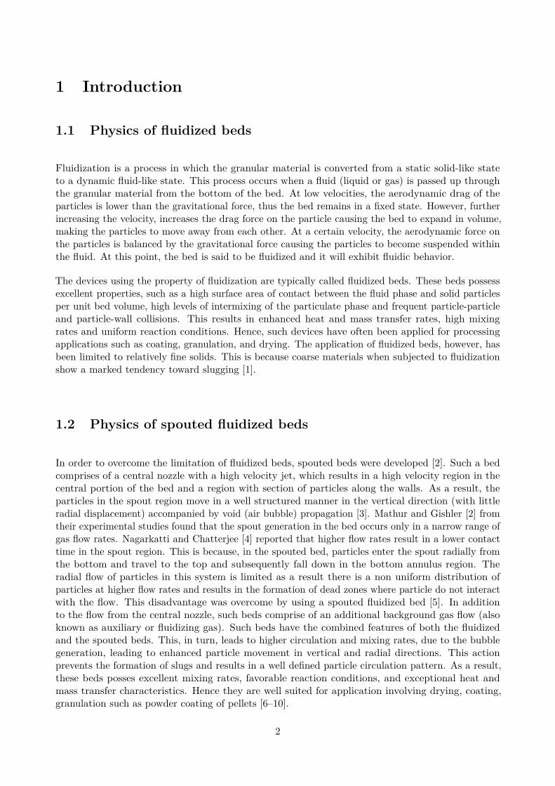
The image of a Wurster bed is shown in Figure (1.1). The Wurster bed consists of several regions,the spray zone, the Wurster column, the horizontal transport region, and the fountain region. Theparticles enter the spray zone through the Wurster column where they collide with the droplets. Thecoated particles get dried by the background air and the dried particles settle down at the bottom ofthe bed in the horizontal transport region. These particles are subjected to the same cycle repetitively.The time taken by a particle to complete one cycle is called the cycle time.

Figure 1.1: Schematic of the Wurster bed coating process along with different zones of interest.

A process like the particle granulation and coating is sensitive to changes in operating conditions.For example, the balance between the evaporation rate and the liquid injection rate is delicate. Ifthe liquid injection rate is too high in comparison to the evaporation rate it can lead to excessagglomeration of particles. However, if the evaporation rate is too high, relative to the injection ratethere is a formation of vapor layer around the particle, which prevents the liquid from sticking to thesurface of the particle (non-wetting contact). As a result of this, heat flux near the surface decreasesdespite high temperature gradient across the surface [21].

Sutkar et al. [22] developed a model for combined heat and mass transfer with liquid injection inwhich both the particles and the droplets are considered as a discrete phase. In their study, theyconsidered the assumption that the collision between the droplet and particle results in a uniformlayer of coating around the particle. The number of particles that were simulated, in this case was82505. Askarishahi et al. [21] modeled liquid injection using the Euler-Lagrangian approach in whichthe droplets were treated as a continuous phase and the particle as a Lagrangian phase. In this model,they incorporated the effect of cooling of the air stream due to the evaporation of droplets from theparticle surface and that of suspended droplets. The surface coverage model did not consider anuniform approach as that of models used by [22] and the coverage model used was that of Kariuki etal. [23]. In their study, the number of particles that were simulated varied from 60,000 to 1,000,000.

A full scale spray simulation for a coating process comprises a complex interplay of the various physicalphenomenon. Since such a simulation requires extensive use of computational resources along withthe need for selecting for suitable models for spray, heat, and the DEM, the number of particles thathave been simulated is limited to few thousand particles. The thesis aims to investigate the processin detail by conducting simulations on a large scale with more than a million particles.

4

1.4 Purpose of the project

In the current project, the in-house developed CFD-DEM tool IPS FluidizationTM from FraunhoferChalmers Centre (FCC) is used to simulate the spouted fluidized bed process, including both heattransfer and a spray phase with evaporation. The software is a state-of-the-art simulation tool withstrong focus on HPC and efficient utilization of both the CPU and the GPU. The constituents of thesoftware is further described below as in Section 1.5. The purpose of the current project was not onthe implementation of the tool, but on the application of the tool.

The project is focused on verification and validation of the tool, as well as investigations of thecurrent practical limits in terms of computational time and system sizes possible to simulate. Theverification is performed in terms of running the software to investigate the previous implementedfeatures of the code, including investigations of the influence of different fields of physics. Whereverpossible, validations are performed against experimental studies from the open literature (for whichthe availability is further discussed below, Section 1.6.

The main target of the software is currently to simulate the pellet coating process for the pharmaceuticalindustry using the mentioned software. In relation to this, the current thesis investigates the feasibilityto study an actual experimental setup for pellet coating process comprises of millions of particles.Whereas in the open literature the maximum number of particles that were simulated in a dryingprocess was limited to 1 million particles with the spray droplets treated as a continuum phase [21],the goal for the current thesis is thus to stretch beyond the mentioned simulation sizes, and alsoinclude a more detailed Lagrangian treatment of the spray parcels as done by IPS FluidizationTM.

In summary, the main objectives of the project are to:

• Model and perform CFD-DEM simulation of a few thousand particles using IPS Fluidizationfor the purpose of validating the solver based on experimental data available in the literature.

• Investigate the coupling between the fluid and the particle using different momentum exchangemodels, convergence studies of the fluid time step and to identify the key parameters influencingthe particle motion in the bed, including friction and rolling friction.

• Perform verification studies on the heat transfer model in IPS Fluidization

• Model and perform industrial scale simulation for the purpose of studying the variation ofcharacteristics of the coated film with the different size distribution of particles.

1.5 Simulation software

The simulation software IPS FluidizationTM is a tool combining the state-of-art CFD multiphasesolver IPS IBOFlow c© [24, 25] and an in-house DEM solver, both developed by FCC. IBOFlow c© haspreviously been used to successfully simulate a number of different industrial applications, such asfiber suspension flow [26, 27], rotary bell spray simulation [28, 29], sealing applications [30, 31], 3Dbioprinting [32] and cases where surface tension play a pivotal role [33]. The in-house DEM solver isa state-of-art solver for both spherical particles and complex shape particles such as rock fragments.The tool include support for arbitrary triangulated domains with models for a range of physicalinteractions. The solver is implemented for massive parallelization on the GPU, with a linear scalingof the solver well above 10 million particles.

IPS FluidizationTM contains a coupling layer which treats the data exchange between the Lagrangian

5

phases (the particles and the spray droplets) and the continuum fields (gas and moisture) in anefficient manner. The data exchange is performed on a generalized grid which is independent of thefluid computational mesh. Due to efficient handling of particle collisions and data interpolation, thetransfer between the GPU (particles and spray) and the fluid fields is minimized. The latter allowsfor a high-resolution coupling with a minimal overhead in terms of simulation time. A schematic ofthe solver is presented in Figure 1.2.

The user interface is implemented via a domain specific language based on Lua. The user sets up andmodels the problem in a combined approach, making the user completely agnostic to the underlyingrecipient of the parameters (DEM or CFD). The Lua layer allows for dynamic result extraction viaprobes, line extraction and also complete data files using the H5 format.

Figure 1.2: Overview of the simulation software, IPS FluidizationTM, including the constituent parts:IPS IBOFlow c©.

1.6 Experimental Data

In this section, the experimental validation data available in the open literature are discussed. Itshould be noted that extensive validation has previously been done at FCC for the separate solvers ofIPS FluidizationTM, and thus the primary aim for the thesis is to find validation data for the coupledsolver.

For validation of momentum transfer between the particles and the fluid, the experimental studiesconducted on a single spout bed by Buijtenen et al. [14] was considered. The study collected thetime-averaged particle velocity fields for the spout-fluidization regime measured using particle imagevelocimetry (PIV) and positron emission particle tracking (PEPT). As such, the data series has beenused extensively in the literature for validation of DEM-CFD solvers [3, 34, 35].

For the heat transfer and the spray models there is an apparent lack of experimental data in theliterature. In many cases the mentioned fields of physics are only verified in qualitative manner [17,18, 21, 22]. Hence, the current project is restricted to verifying the cases using simple 1D models as abasis.

6

As a preparatory step for the industrial scale simulation, a validation of the input parameters thatare needed for a large scale pilot simulation, studies are performed on a small scale setup based onthe experimental studies conducted by Liang et al. [36].

1.7 Structure of the thesis

The rest of the chapters in this thesis are structured as follows

• In Chapter 2, the different CFD and DEM models along with their coupling scheme are presented.

• In Chapter 3, the DEM-CFD methodology and the coupling strategies are discussed.

• In Chapter 4, the description of various simulation cases are given.

• Finally, in Chapter 5, the results of various simulations are presented and discussed.

7

2 Theory

The CFD-DEM method is used to model systems comprising of a fluid and a solid phase (for earlyuses of the method see e.g. developed by Tsuji et al. [12]). The fluid phase is solved using the CFDtechnique, in which the gas phase is treated as a continuum phase based on the Eulerian approach,with conservation equations formulated for all fields of physics (Section 2.1).

The particles are considered as a discrete phase and treated based on the Lagrangian approach andsolved using DEM. In this approach, each particle is tracked individually and their positions, velocities,etc are described as a function of time. Furthermore, the collisions between particles and particlesand walls are resolved in a so-called soft sphere manner. The DEM approach is further described inSection 2.2. In addition, the Lagrangian droplet phase is described in Section 2.3.

Since the fluid phase and solid phase are treated in different mathematical frames of references, thecoupling terms are of profound importance in CFD-DEM. In general, the coupling between the fluidand the solid phase happens in a two way approach, i.e., the fluid field influences the particles andparticles, in turn, affects the fluid. The coupling between the particles and fluid is further describedin Section 2.4.

2.1 Computational Fluid Dynamics

Computational Fluid Dynamics is the analysis of systems involving fluid flow, heat transfer andassociated phenomena with the help of computers. This method comprises of three main steps whichare described below [37].

• Integration of the governing equations of fluid flow over all the (finite) control volumes of thedomain.

• Discretization – conversion of the resulting integral equations into a system of algebraic equations.

• Solution of the algebraic equations by an iterative method.

Thus it is essential to describe the governing equations for the gas phase dynamics before it couldbe discretized into algebraic equations. For the current applications, the gas phase is treated as anincompressible Newtonian fluid. The model for the gas phase is described using the volume averagedNavier-Stokes equations, where all variables are locally averaged over the control volume. Theseequations describe how the velocity, pressure, temperature, and density of a moving fluid are related.

2.1.1 Mass and momentum conservation

The governing equation for the conservation of mass is given by the continuity equation as follows,

∂(εfρf )∂t

+ O.(εfρfuf ) = 0. (2.1)

Newton’s second law states that the rate of change of momentum of a fluid phase equals the sum ofthe forces on the particle. The forces may be surface forces or body forces. The governing equationdescribing the action of such forces on the fluid phase is given by the momentum equation. Themomentum equation for the fluid phase is given as follows [34],

∂εfρfuf

∂t+ O.(εfρfufuf ) = −εfOp− O.(εfτf ) + Sp + εfρfg, (2.2)

8

where ρf is the density of the gas phase, τf is the gas phase stress tensor, uf is the velocity of thegas phase and g is the gravitational acceleration constant. The gas phase stress tensor is calculatedas follows,

τf = −µf((Ouf ) + (Ouf )T

)+ 2

3µfO.ufδ, (2.3)

where µf denotes the viscosity of the gas phase. Sp denotes the source term for coupling themomentum transfer from the particulate phase and will be described in detail in the coupling section(Section 2.4).

2.1.2 Heat transfer

Since the process of particle coating involves drying of the solvent that is deposited over the particlephase it is essential to include models for heat transfer. The applied thermal energy equation for thegas phase as proposed by Syamlal and Gidaspow [38] is given by:

∂(εfρfCp,fT )∂t

+ O.(εfρfufCp,fT ) = O.(εfkfOT ) + Sh, (2.4)

where Sh represents the source term for heat coupling with the particulate phase and will be describedin detail in Section 2.4.2. Cp,f is the fluid heat capacity and kf is the thermal conductivity of the gasphase.

2.1.3 Moisture conservation equation

The particles are moistened when hit by the spray droplets. Due to the heated fluidization air, thesolute evaporates from the particles and is convected by the air. The conservation equation describingthe transport of the moisture (wf ) is given by [22],

∂εfρfwf∂t

+ O.(εfρfufwf ) = −O.(εqm) + Sm, (2.5)

where the term qm represents the mass transfer flux which is described in terms of the gas diffusivity(Df ) such that:

qm = DfOwf , (2.6)and Sm is the source term for coupling the mass transfer between fluid and the particulate.

2.2 Discrete Element Method

DEM is a particle-scale numerical method for modeling the bulk behavior of granular materials [13].Each particle is represented by its specific properties such as its size, shape, velocity and angularvelocity. The particles are subjected to forces due to gravity, momentum exchange with the fluid,particle-particle interaction and particle-wall contact forces. The trajectories of the particles areexplicitly solved using Newton’s second law of motion under small incremental steps in time. Inpractical terms, this requires solving one ODE per state variable (position, velocity and angularvelocity) and per time step.

The process is represented in Figure (2.1). In Figure (2.1), a particle tends to come in contact withother particles, as a result, it experiences force from other particles. Forces from fluid phase andgravity are also included in this step. The net force acting on the particle is calculated and theparticle state is updated using Newton’s second law.

9

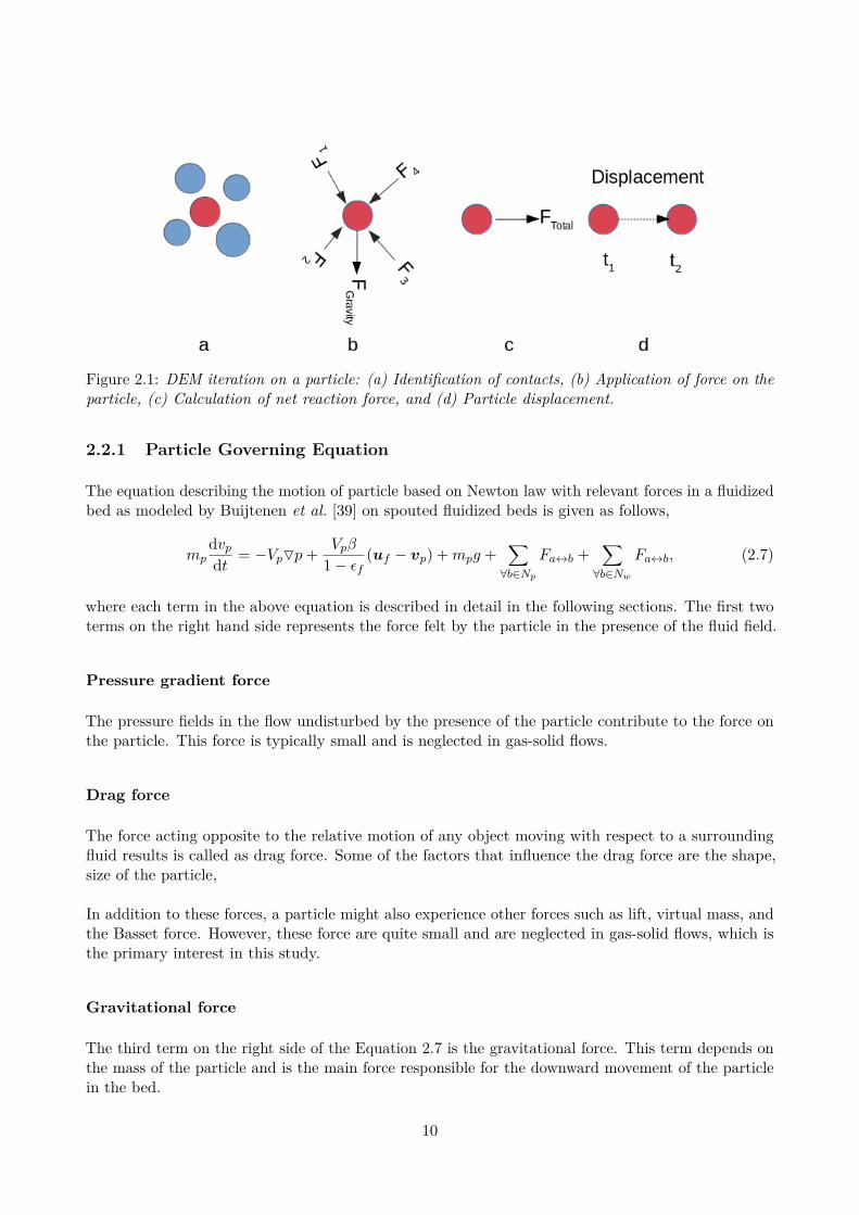
Figure 2.1: DEM iteration on a particle: (a) Identification of contacts, (b) Application of force on theparticle, (c) Calculation of net reaction force, and (d) Particle displacement.

2.2.1 Particle Governing Equation

The equation describing the motion of particle based on Newton law with relevant forces in a fluidizedbed as modeled by Buijtenen et al. [39] on spouted fluidized beds is given as follows,

mpdvpdt = −VpOp+ Vpβ

1− εf(uf − vp) +mpg +

∑∀b∈Np

Fa↔b +∑∀b∈Nw

Fa↔b, (2.7)

where each term in the above equation is described in detail in the following sections. The first twoterms on the right hand side represents the force felt by the particle in the presence of the fluid field.

Pressure gradient force

The pressure fields in the flow undisturbed by the presence of the particle contribute to the force onthe particle. This force is typically small and is neglected in gas-solid flows.

Drag force

The force acting opposite to the relative motion of any object moving with respect to a surroundingfluid results is called as drag force. Some of the factors that influence the drag force are the shape,size of the particle,

In addition to these forces, a particle might also experience other forces such as lift, virtual mass, andthe Basset force. However, these force are quite small and are neglected in gas-solid flows, which isthe primary interest in this study.

Gravitational force

The third term on the right side of the Equation 2.7 is the gravitational force. This term depends onthe mass of the particle and is the main force responsible for the downward movement of the particlein the bed.

10

Particle-particle interaction force

The fourth term on the right side of the Equation 2.7 represents the particle-particle interaction force.In dense flows, the loss of kinetic energy by inter-particle collisions is high and hence, it is important.The soft sphere model developed by Cundall and Strack [13] is typically applied in DEM. This modeltreats particle-particle collisions as finite overlaps. In this model, particles are typically assumed toremain geometrically rigid during contact. The deformation of the particle during the collision isassumed to be small.

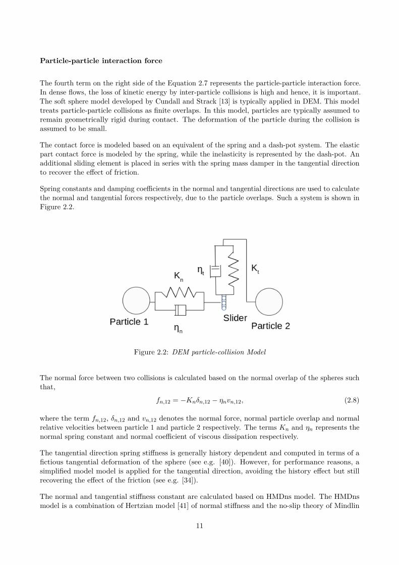
The contact force is modeled based on an equivalent of the spring and a dash-pot system. The elasticpart contact force is modeled by the spring, while the inelasticity is represented by the dash-pot. Anadditional sliding element is placed in series with the spring mass damper in the tangential directionto recover the effect of friction.

Spring constants and damping coefficients in the normal and tangential directions are used to calculatethe normal and tangential forces respectively, due to the particle overlaps. Such a system is shown inFigure 2.2.

Figure 2.2: DEM particle-collision Model

The normal force between two collisions is calculated based on the normal overlap of the spheres suchthat,

fn,12 = −Knδn,12 − ηnvn,12, (2.8)

where the term fn,12, δn,12 and vn,12 denotes the normal force, normal particle overlap and normalrelative velocities between particle 1 and particle 2 respectively. The terms Kn and ηn represents thenormal spring constant and normal coefficient of viscous dissipation respectively.

The tangential direction spring stiffness is generally history dependent and computed in terms of afictious tangential deformation of the sphere (see e.g. [40]). However, for performance reasons, asimplified model model is applied for the tangential direction, avoiding the history effect but stillrecovering the effect of the friction (see e.g. [34]).

The normal and tangential stiffness constant are calculated based on HMDns model. The HMDnsmodel is a combination of Hertzian model [41] of normal stiffness and the no-slip theory of Mindlin

11

[42] for the tangential stiffness. The normal stiffness in this model is given as follows,

kn = 43E∗√Rδn, (2.9)

where the term E∗ is calculated as follows,

E∗ = E

2(1− ν2) , (2.10)

based on Young’s modules (E) and Poisson’s ratio (ν). The stiffness of the particles also affects thespring force and the collision time.

The last term on the right side of the Equation 2.7 represents the interaction force between the walland the particle. This interaction is treated in the same way as particle-particle interaction, with thewall having zero velocity.

The particle also experiences rotation in a bed in addition to translation. This is given by theangular momentum equation, one main assumption in this equation is that the torque is solely dueto particle-particle contact and not due to fluid-particle interaction. The equation describing therotation of a spherical particles is given as follows,

Ipdωpdt =

∑Np

Mp, (2.11)

where ωp is particle angular velocity, Mp is the torque, and Ip is the moment of inertia.

In addition to the above described forces, the model also includes a rotational friction term givingrise to a momentum on the particle such that[43]:

Mr = − ωrel|ωrel|

µrRfn (2.12)

where ωrel is the relative rotational velocity between two particles or between a particle and the wall.The induced moment contributes to Mp above.

2.2.2 Heat transfer Model

Various modes of heat transfer manifest in a system with gas-solid flows. The particulate phase, inprincipal experiences particle-particle and particle-wall heat conduction, convective heat transferwith the surrounding gas, particle-particle/wall frictional heating and radiative heat transfer withthe surrounding gas and bed walls. Heat transfer through radiation is significant only for hightemperatures (typically > 700 K). The mode and the rate of heat transfer are dependent on thesystem of application and its flow characteristics and the following assumptions are considered here:

• Conductive heat transfer between particle-particle and particle-wall were neglected. Thisassumption is valid if particles are in free flight all the time which is true in case of fluidizedsystems.

• Radiative heat transfer is neglected as the absolute temperature is relatively low (less than100◦C)

Base on those assumptions, the heat balance equation for a particle p, as used by Patil et al. [17] intheir work on heat transfer is given as follows,

ρpVpCp,pdTpdt = hfpAp(Tf − Tp), (2.13)

12

where Tf is the fluid temperature, Ap is effective area of the particle available for heat transfer andCp,p is the particle heat capacity. This equation incorporates heat transfer between fluid and gasphase through convection. The term hfp represents the heat transfer co-efficient between the gas andthe particles evaluated using the empirical Nusselt number correlation as given by Gunn [44],

Nup = (7− 10εf + 5ε2f )[1 + 0.7Re0.2p Pr0.33] + (1.33− 2.40εf + 1.20ε2f )Re0.7

p Pr0.33, (2.14)

where the terms Rep and Pr denote the particle Reynold’s number and Prandtl number respectively.They are calculated as follows,

Rep = ρf εfdp | uf − vp |µf

, (2.15)

Pr = µfCpfkf

, (2.16)

and the term Nup is the Nusselt number (which is the ratio of convective to conductive heat transferat a boundary in a fluid) is used to calculate heat transfer co-efficient as follows,

hfp = Nupkfdp

. (2.17)

2.2.3 Mass transfer model

In the current application, the spray phase is, after deposition on the particles, evaporated fromthe particle surface to the surrounding fluid. The driving force for evaporation is the difference inconcentration of the droplet vapor between the particle surface and the free stream. Under the currentassumption of a uniform layer of spray solid and spray liquid over the particle, the equation describingthe transfer of mass from the liquid phase to the gas phase is given as follows [22],

dmp

dt = kmAp(w∗f − wf ), (2.18)

where the term km denotes the mass transfer coefficient for the gas phase which is a proportionalityconstant that relates the mass transfer rate and change in concentration of moisture content as drivingforce. Further, the term w∗f denotes the saturated concentration of liquid at the solid-liquid interface.In a two component system, a thermodynamic equilibrium exits at the gas-liquid interface. Hence,the term w∗f at the interface can be calculated as follows,

w∗f = mdXd,s

mdXd,s +mf (1−Xd,s), (2.19)

where Xd,s is the mole fraction of moisture at the particle surface mf and md are the molecularweights of surrounding gas and surrounding droplet respectively. The mole fraction of moisture atthe particle surface is described by Clausius Clapeyron equation, by assuming a thermodynamicequilibrium at the gas-liquid interface. The term is given as follows,

Xd,s = PrefPamb

exp

(4Hatm

(1

Tb,atm− 1Td,s

)md

R

)), (2.20)

and is calculated based on ambient pressure pamb and the reference pref with 4Hevap being theevaporation enthalpy defined at reference pressure and the boiling temperature at reference pressureTb,ref , R is the universal gas constant and md is the molar mass of the moisture.

13

The effect of a relative velocity between the droplet and the conveying gas is to increase the evaporationor condensation rate. This effect is represented in [44] using the Sherwood correlation as follows,

Shp = (7− 10εf + 5ε2f )[1 + 0.7Re0.2p Pr0.33] + (1.33− 2.40εf + 1.20ε2f )Re0.7

p Sc0.33, (2.21)where Sc being the Schmidt number is used to characterize fluid flows in which there is simultaneousmomentum and mass diffusion convection processes calculated based on the viscosity, density anddiffusivity of the gas phase as follows,

Sc = µfDfρf

. (2.22)

The mass transfer coefficient is evaluated based on the Sherwood number correlation calculated basedon the Equation 2.21, gas diffusivity Df and particle diameter as follows,

Km = ShpDf

dp. (2.23)

2.3 Spray droplets

The spray droplets are a mixture of spray solid and the spray fluid. The purpose of having the spray inthe simulation is to simulate the coating process. Since the individual collision between the particlesand the droplets needs to be resolved it is essential to track the droplets in a Lagrangian sense. In thecurrent framework, the collisions between the droplets are not resolved, i.e., no two droplets collidewith each other. Furthermore, the spray is currently assumed to have a one way interaction withthe gas phase, i.e., the droplets experience the force from the fluid through the momentum exchangeterm. However the presence of droplet does not affect the gas phase itself. Such an assumption isvalid under low spray loadings.

Further, the droplets are simulated under the assumption of low droplet Weber number, such that anybreakage of the droplets can be neglected. This assumption is reasonable since most droplet breakagetakes place in a very small region close to the nozzle, after which the droplets are small enough tokeep their size. The characteristic sizes of the droplets are to be chosen based on size representablefor the spray after the initial breakup.

In a droplet particle collision, it is assumed that the droplets are completely captured by the particles.This assumption is valid in cases with a small droplet to particle diameter ratio. As mentioned above,a captured droplet is assumed to form a uniform liquid layer around the particle. In the currentapproach, the droplets will not alter the characteristics of the particles, e.g, not increasing the massof the particles, which is reasonable for small spray loadings applied under a short simulation time.Finally, it is assumed that the droplets have the same temperature as that of the gas phase andalso there is no evaporation from the droplets present in the gas phase, which is again a reasonableassumption if the time from injection to collision is short.

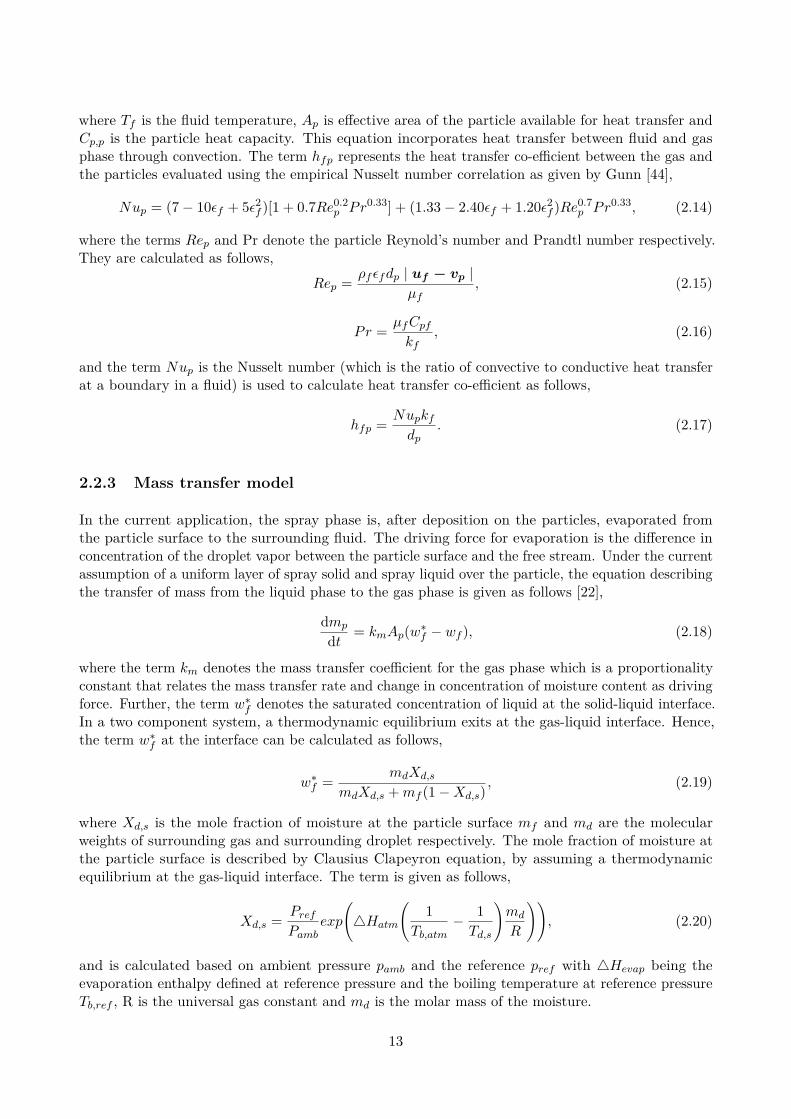
An outline of the spray process is shown in Figure 2.3. The droplets are a mixture of a spray solid(red colour) and spray liquid (blue colour). When the droplets collide with the particles (black colour)they droplets are removed from the simulation in the gas phase and get deposited on to the particle.The moisture evaporates and the coating (spray-solid) is left on the particles.

2.4 Multiphase Coupling

As touched upon in the previous sections, the fluid and the particles are coupled via the exchange ofmomentum, energy and mass.

14

Figure 2.3: Spray process from a spray cone injector, with R as the radius and A as the cone angle.

In general, a coupling between the particles and the gas depends on the particle size, the relativevelocity and the volume fraction of the solid phase. From an exchange point of view there are threetypically considered classes of problems:

• One way coupling: This type of coupling is mainly present in sufficiently dilute flows such thatfluid feels no effect from the presence of particles. In this type of flow, particles move in dynamicresponse to the fluid motion (See Figure 2.4.a).

• Two way coupling: If enough particles are present in the fluid phase, such that the momentumexchange between dispersed and carrier phase interfaces alters dynamics of the carrier phase, itis essential to model a two way coupling between the carrier phase and the particle phase (SeeFigure 2.4.b).

• Four way coupling: If the flow is dense enough, the effect of dispersed phase collisions aresignificant. In such a situation there is a need for four way coupling. In a four way coupling, thefluid field affects the dispersed phase, the dispersed phase in turn affect the fluid, in addition tothat, there is an interaction between the dispersed phase (See Figure 2.4.c).

The three types of coupling mechanism are shown in the Figure 2.4,

In a system such as the fluidized bed, there is interaction between the dispersed phase, as well asinteraction with the fluid phase, essentially requiring four way coupling. The coupling between theparticle-particle and particle-wall interaction is described in the Section 2.2.1. In this section, differentinterphase coupling mechanism such as the momentum, energy and mass will be described in detail.

2.4.1 Momentum Exchange

The coupling between the fluid and the dispersed phase happens through the interphase momentumexchange term in the momentum Equation 2.2 for the fluid and for the particle Equation 2.7. Inorder to couple the fluid and the dispersed phase, it is essential to calculate the volume fraction ofparticle present in each cell. The particle volume fraction is calculated by measuring the fraction of

15

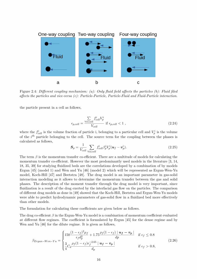
Figure 2.4: Different coupling mechanism: (a): Only fluid field affects the particles (b): Fluid filedaffects the particles and vice-versa (c): Particle-Particle, Particle-Fluid and Fluid-Particle interaction.

the particle present in a cell as follows,

εp,cell =

∑∀i∈cell

f icellVip

Vcellif εp,cell < 1 , (2.24)

where the f icell is the volume fraction of particle i, belonging to a particular cell and V ip is the volume

of the ith particle belonging to the cell. The source term for the coupling between the phases iscalculated as follows,

Sp = 1Vcell

∑∀i∈cell

f icellβipV

ip (uf − vip). (2.25)

The term β is the momentum transfer co-efficient. There are a multitude of models for calculating themomentum transfer co-efficient. However the most predominantly used models in the literature [3, 14,18, 35, 39] for studying fluidized beds are the correlations developed by a combination of by modelsErgun [45] (model 1) and Wen and Yu [46] (model 2) which will be represented as Ergun-Wen-Yumodel, Koch-Hill [47] and Beetstra [48]. The drag model is an important parameter in gas-solidinteraction modeling as it allows to determine the momentum transfer between the gas and solidphases. The description of the moment transfer through the drag model is very important, sincefluidization is a result of the drag exerted by the interfacial gas flow on the particles. The comparisonof different drag models as done in [49] showed that the Koch-Hill, Beetstra and Ergun-Wen-Yu modelswere able to predict hydrodynamic parameters of gas-solid flow in a fluidized bed more effectivelythan other models.

The formulation for calculating these coefficients are given below as follows.

The drag co-efficient β in the Ergun-Wen-Yu model is a combination of momentum coefficient evaluatedat different flow regimes. The coefficient is formulated by Ergun [45] for the dense regime and byWen and Yu [46] for the dilute regime. It is given as follows,

βErgun−Wen−Y u =

150(1− εf )2µf

εfd2p

+ 1.75ρf (1− εf ) | uf − vp |dp

if εf ≤ 0.8

34Cd

ρf (1− εf )ε−2.65f | uf − vp |dp

if εf > 0.8,(2.26)

16

where Cd is the drag coefficient formulated based on the particle Reynolds’s number as follows,

Cd =

24Rep

(1 + 0.15Re0.687p ) (Rep ≤ 1000)

0.44 (Rep > 1000).(2.27)

The momentum transfer coefficients due to drag as given by Hill et al. [47], is calculated using a dragrelation proposed by Koch and Hill (2001) again based on lattice-Boltzmann simulations which worksin the same Reynolds’s number range as 1000 as given in [48]. It is given as follows,

βKoch−Hill =18µf ε2f (1− εf )

d2p

(F0 + 1

2F3Rep

), (2.28)

where the coefficients F0 and F3 are based on the fluid volume fractions. The term F0 is calculated asfollows,

Fo =

1 + 3

√(1− εf )

2 + 13564 (1− εf )ln(1− εf ) + 16.1(1− εf )

1 + 0.68(1− εf )− 8.48(1− εf )2 + 8.16(1− εf )3 if (1− εf ) < 0.4

10(1− εf )ε3f

if (1− εf ) ≥ 0.4

, (2.29)

and the term F3 is calculated as follows,

F3 = 0.0673 + 0.212(1− εf ) + 0.0232ε5f

. (2.30)

The momentum transfer coefficient as given by Beetstra et al. [48] was formulated based on the latticeBoltzmann simulations. This model works well upto a Reynolds’s number range of 1000 which is thesame as in Koch-Hill model.

βBeetstra = K1µf(1− εf )2

d2pεf

+K2µfεpRepd2p

, (2.31)

where K1, K2 are coefficients which are dependent on the volume fraction of the two phases and theReynolds’s number given as follows,

K1 = 180 + 18ε4fεp

(1 + 1.5√εp), (2.32)

K2 = 0.31ε−1f + 3εf (1− εf ) + 8.4Re−0.343

p

1 + 103(1−εf )Re2εf−2.5p

. (2.33)

2.4.2 Energy exchange between the phases

There is a two way coupling in terms of heat transfer between the fluid and the particle phase. Thefluid to particle heat transfer is found by summing the contributions of all particles belonging to aparticular Eulerian cell. The source term for the heat exchange Sh is given as follows by the Equation2.4,

Sh =

∑∀i∈cell

f icellhfp(Tp,i − Tf,p)

Vcell, (2.34)

where the term Tf,p denotes the temperature of fluid at the particle location, Tp,i represents thetemperature of the i-th particle belonging to a cell.

17

2.4.3 Mass exchange between the phases

The spray liquid from the droplets that are deposited over the surface of the particle will get vaporizedand get converted into moisture phase in the presence of heat. The rate of evaporation is dependenton the difference in concentration of the moisture content between the gas phase and the surfaceof the particle. The evaporation is also dependent on the surface area of the particle available forevaporation. The expression for coupling between the two phases is given as follows,

Sm =

∑∀i∈cell

f icellkmAp(w∗f − wf )

Vcell. (2.35)

18

3 Methodology

This Chapter explains the different methodologies used in the project, describing parts of theimplementation and discretization as provided in the IPS Fluidization software. This chapter isdivided into three different sections. In the Section 3.1, a brief description of the CFD solutionprocedure is given, followed by Section 3.2 on DEM algorithm and finally in Section 3.3, the couplingstrategies are explained.

3.1 CFD solution procedure

In this section, the procedure used by fluid flow solver IBOFlow c© to solve for the flow variablesis explained. IBOFlow is based on a unique immersed boundary technique using the finite volumemethod to discretize the equations on a Cartesian octree grid which can be dynamically refined andcoarsened. The solver works on a segregated approach. The Navier Stoke Equations (see Equation 2.1and Equation 2.2) are first solved using the SIMPLEC method, for more information about thismethod refer [50]. The temperature is solved using the Equation 2.4. The interpolation schemeby Rhie and Chow [51] is used. The implicit Euler scheme is used for time integration, as it isunconditionally stable. Finally, for the convective terms, the Ultimate quickest scheme, which is thirdorder accurate in space, is used. Due to the immersed boundary technique no a priori meshing isrequired.

3.2 DEM algorithm

In this section, the DEM algorithm is described. A flow chart describing the general DEM algorithmis shown in Figure 3.1. There are different steps involved in the DEM algorithm. In the first step,the location and the size distribution of the particles are defined by the user. The are differentpossible ways of describing such an arrangement. The two ways of particle arrangement availablein the solver, IPS FluidizationTM, are the cylindrical and the box arrangement. The image of twosuch arrangements is shown in Figure 3.2. The solver IPS Fluidization has the possibility to modelparticles of the same size or even have particles of different sizes.

The second step involved is to identify the collisional neighbors. This is done by sorting the list ofparticles based on their position in combination with a highly-efficient data structure for indexingnearest neighbours. The collisional detection in IPS Fluidization is developed to work in the massivelyparallel environment of the GPU (further discussed in Section 3.3.2) and allows for a linear scaling ofthe computational time for millions of particles. The actual algorithm of the software is not disclosed.

Next, the forces between the particles are calculated based on the soft sphere approach as explainedin Section 2.2.1. In the next step, other forces such as the drag and gravity are calculated and areadded to the existing forces, in addition, torque on the particles is also calculated. Using the forcesthat are acting on the particles, the acceleration, the velocity, angular velocity and its position areevaluated by integrating the equation on a smaller time step.

19

Figure 3.1: Flowchart of the DEM Algorithm.

(a) Box arrangement (b) Cylinder Arrangement

Figure 3.2: Different Particle arrangements as available in the IPS Fludization.

3.3 Coupling method

DEM alone is computationally expensive, it is essential to accelerate the performance for the purposeof reducing the simulation time. Accelerating the performance of the simulation was previouslyperformed in Central Processing Unit (CPU) by increasing the number of CPU cores. However,this can lead to reduced performance of coupled CFD-DEM simulations due to increase in global

20

communication overhead in comparison to standalone DEM and CFD simulation as shown in [52].

As an alternative, the GPU, initially developed to render images, have recently been used to performintensive mathematical calculations for computational purposes in science and technology becauseof its massive parallel processing capabilities. The efficient architecture of the GPU allows one toperform multiple calculations at the same time. As an example, Radeke et al. [53] utilized the powerof GPUs to successfully simulate millions of particles. Thus a combination of CFD running on CPUand DEM running on GPU allows us to effectively parallelize the CFD-DEM simulations.

The GPU approach is heavily used in IPS FluidizationTM, where all particle and spray computationsare performed solely on the GPU.

3.3.1 Data transfer

The are two ways of generating a mesh in a CFD-DEM simulation. The first way is by using a singlemesh for both the fluid and the particles. The other method is by using a separate mesh for both thefluid and the particles. Generally, fine grids are required to resolve the fluid flow field requirementsas the accuracy of the simulation is dependent on the appropriate cell size. Decreasing the cell sizecan improve the accuracy of the result, however, can result in increased computational time. Themain need for using fine grids is to resolve the geometrical features which influence the flow field.However, using a fine grid can affect the particle field resolution requirements. Especially in cases,where particle concentration is low inside a computational cell, as sharp changes in the solid volumefraction can happen leading to numerical instabilities. One can overcome this problem by usingseparate meshes for both the fluid and the particles. In this method, the particles are tracked througha course grid while the fluid field has a finer grid, thus, overcoming the disadvantages of using a singlegrid.

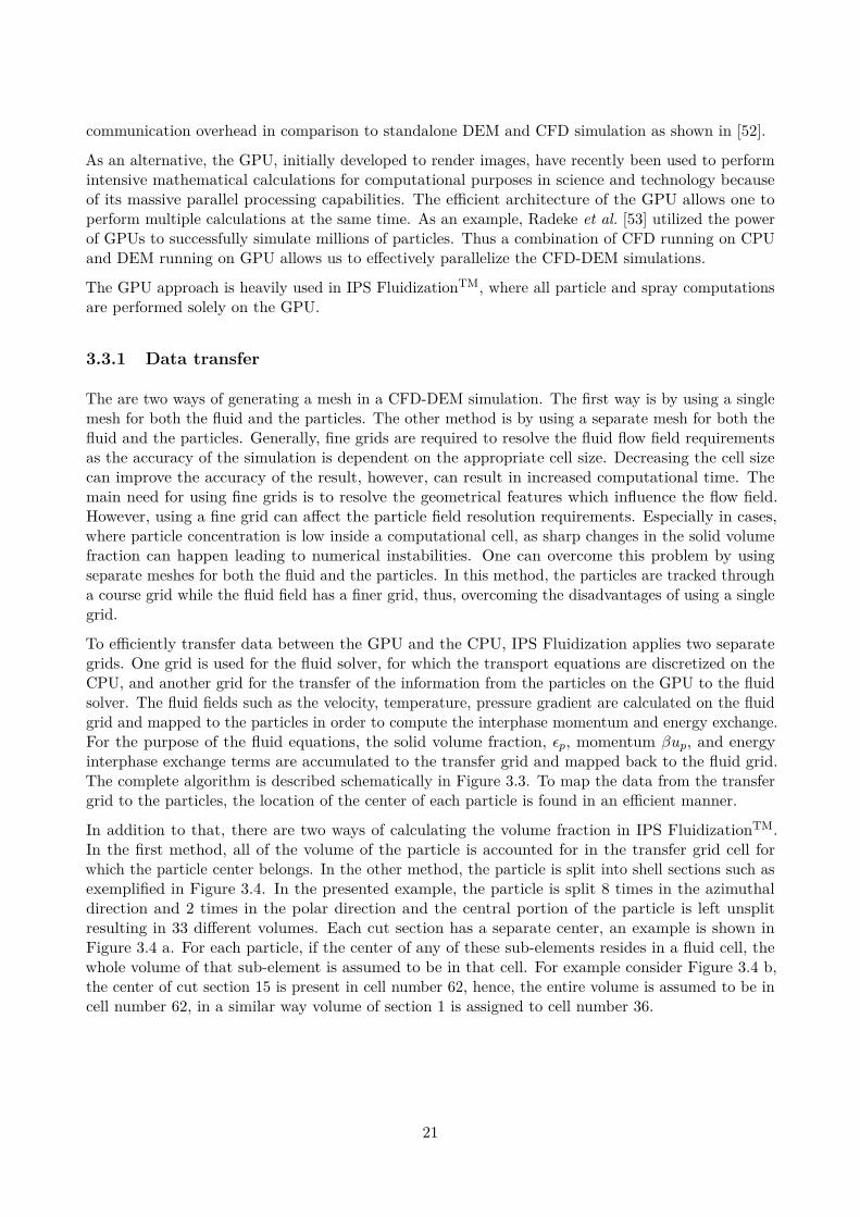
To efficiently transfer data between the GPU and the CPU, IPS Fluidization applies two separategrids. One grid is used for the fluid solver, for which the transport equations are discretized on theCPU, and another grid for the transfer of the information from the particles on the GPU to the fluidsolver. The fluid fields such as the velocity, temperature, pressure gradient are calculated on the fluidgrid and mapped to the particles in order to compute the interphase momentum and energy exchange.For the purpose of the fluid equations, the solid volume fraction, εp, momentum βup, and energyinterphase exchange terms are accumulated to the transfer grid and mapped back to the fluid grid.The complete algorithm is described schematically in Figure 3.3. To map the data from the transfergrid to the particles, the location of the center of each particle is found in an efficient manner.

In addition to that, there are two ways of calculating the volume fraction in IPS FluidizationTM.In the first method, all of the volume of the particle is accounted for in the transfer grid cell forwhich the particle center belongs. In the other method, the particle is split into shell sections such asexemplified in Figure 3.4. In the presented example, the particle is split 8 times in the azimuthaldirection and 2 times in the polar direction and the central portion of the particle is left unsplitresulting in 33 different volumes. Each cut section has a separate center, an example is shown inFigure 3.4 a. For each particle, if the center of any of these sub-elements resides in a fluid cell, thewhole volume of that sub-element is assumed to be in that cell. For example consider Figure 3.4 b,the center of cut section 15 is present in cell number 62, hence, the entire volume is assumed to be incell number 62, in a similar way volume of section 1 is assigned to cell number 36.

21

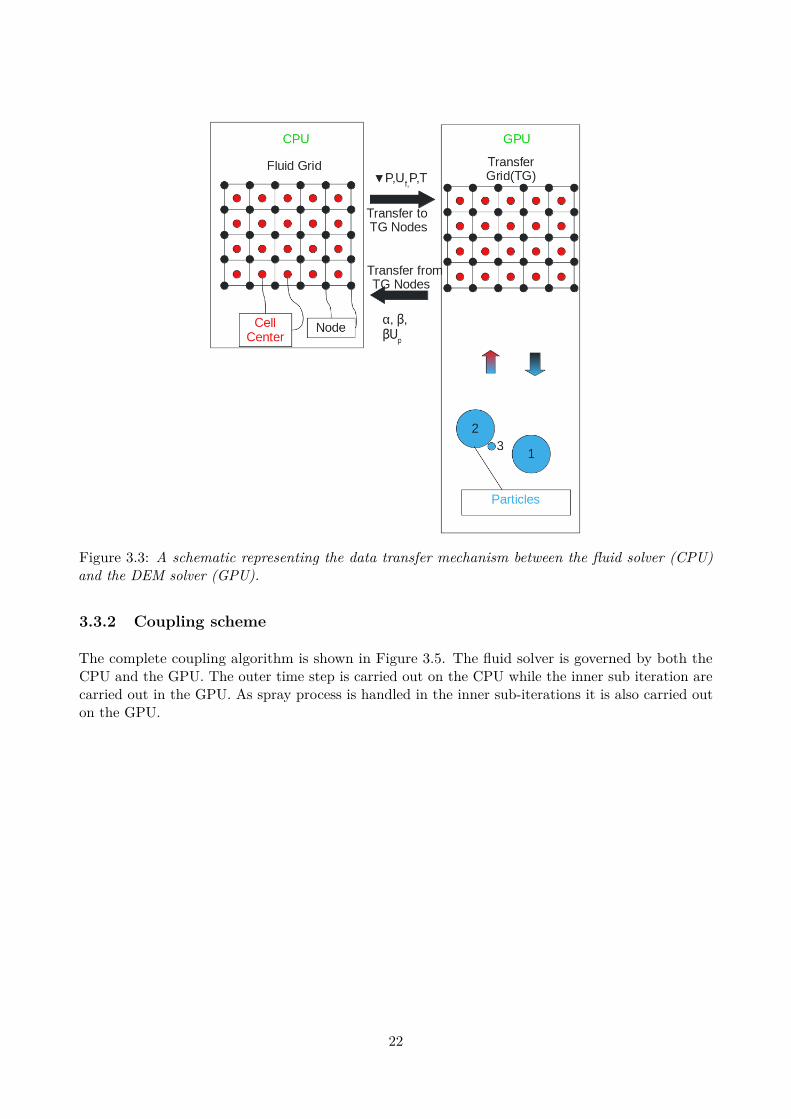
Figure 3.3: A schematic representing the data transfer mechanism between the fluid solver (CPU)and the DEM solver (GPU).

3.3.2 Coupling scheme

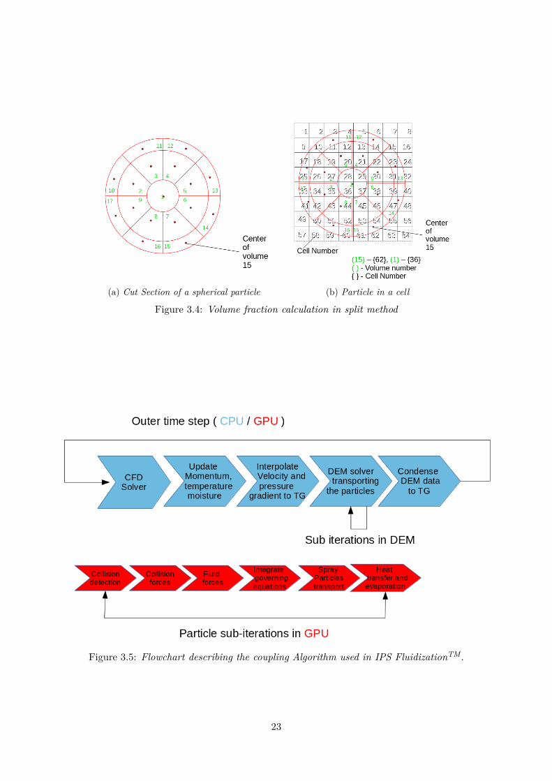
The complete coupling algorithm is shown in Figure 3.5. The fluid solver is governed by both theCPU and the GPU. The outer time step is carried out on the CPU while the inner sub iteration arecarried out in the GPU. As spray process is handled in the inner sub-iterations it is also carried outon the GPU.

22

(a) Cut Section of a spherical particle (b) Particle in a cell

Figure 3.4: Volume fraction calculation in split method

Figure 3.5: Flowchart describing the coupling Algorithm used in IPS FluidizationTM.

23

4 Simulation cases

In this Chapter, the different simulations that are performed in the project are described, givingcomplete details of the geometry, mesh and the solver settings. This Chapter is divided into threesections. In the Section 4.1, the settings used for performing single spout bed are described. In theSection 4.2, the description of the 1-D simulation setup that was used for performing the verificationof the heat transfer model is given. Finally, in the Section 4.3, the details pertaining to the spraycoating simulation are specified.

4.1 Single Spout Bed simulation

In order to validate the coupled CFD-DEM solver, it is essential to compare the simulation resultswith the experimental results. For this purpose, experimental studies conducted on a single spout bedusing PEPT and PIV by Buijtenen et al. [14] are considered. In this section, the complete descriptionof the geometrical setup along with the various numerical settings that are used for the simulationare described in detail.

4.1.1 Geometry of the single spout bed

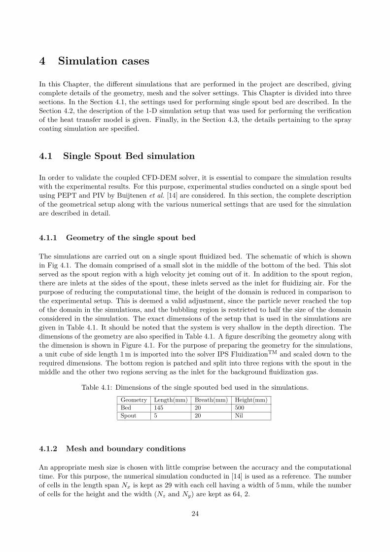
The simulations are carried out on a single spout fluidized bed. The schematic of which is shownin Fig 4.1. The domain comprised of a small slot in the middle of the bottom of the bed. This slotserved as the spout region with a high velocity jet coming out of it. In addition to the spout region,there are inlets at the sides of the spout, these inlets served as the inlet for fluidizing air. For thepurpose of reducing the computational time, the height of the domain is reduced in comparison tothe experimental setup. This is deemed a valid adjustment, since the particle never reached the topof the domain in the simulations, and the bubbling region is restricted to half the size of the domainconsidered in the simulation. The exact dimensions of the setup that is used in the simulations aregiven in Table 4.1. It should be noted that the system is very shallow in the depth direction. Thedimensions of the geometry are also specified in Table 4.1. A figure describing the geometry along withthe dimension is shown in Figure 4.1. For the purpose of preparing the geometry for the simulations,a unit cube of side length 1 m is imported into the solver IPS FluidizationTM and scaled down to therequired dimensions. The bottom region is patched and split into three regions with the spout in themiddle and the other two regions serving as the inlet for the background fluidization gas.

Table 4.1: Dimensions of the single spouted bed used in the simulations.Geometry Length(mm) Breath(mm) Height(mm)Bed 145 20 500Spout 5 20 Nil

4.1.2 Mesh and boundary conditions

An appropriate mesh size is chosen with little comprise between the accuracy and the computationaltime. For this purpose, the numerical simulation conducted in [14] is used as a reference. The numberof cells in the length span Nx is kept as 29 with each cell having a width of 5 mm, while the numberof cells for the height and the width (Nz and Ny) are kept as 64, 2.

24

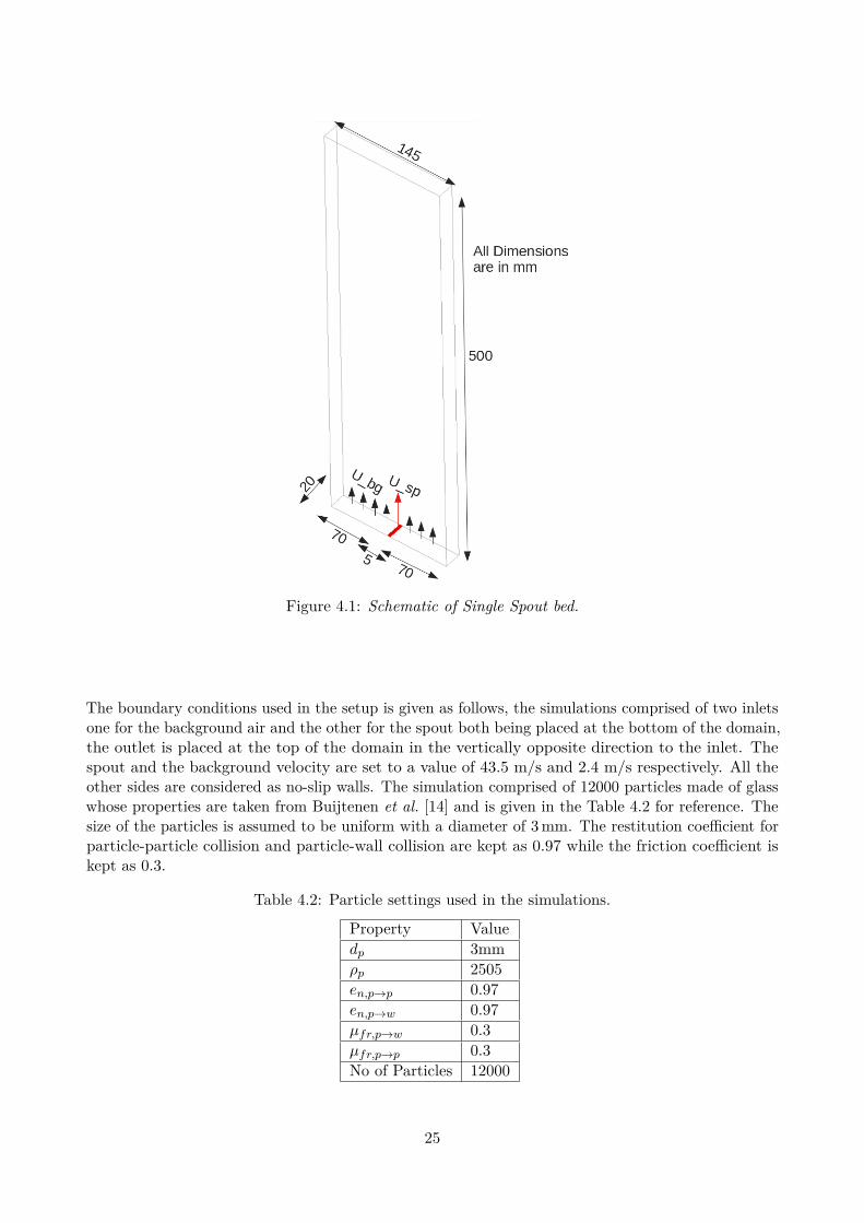
Figure 4.1: Schematic of Single Spout bed.

The boundary conditions used in the setup is given as follows, the simulations comprised of two inletsone for the background air and the other for the spout both being placed at the bottom of the domain,the outlet is placed at the top of the domain in the vertically opposite direction to the inlet. Thespout and the background velocity are set to a value of 43.5 m/s and 2.4 m/s respectively. All theother sides are considered as no-slip walls. The simulation comprised of 12000 particles made of glasswhose properties are taken from Buijtenen et al. [14] and is given in the Table 4.2 for reference. Thesize of the particles is assumed to be uniform with a diameter of 3 mm. The restitution coefficient forparticle-particle collision and particle-wall collision are kept as 0.97 while the friction coefficient iskept as 0.3.

Table 4.2: Particle settings used in the simulations.

Property Valuedp 3mmρp 2505en,p→p 0.97en,p→w 0.97µfr,p→w 0.3µfr,p→p 0.3No of Particles 12000

25

4.1.3 Physics Modelling and result extraction

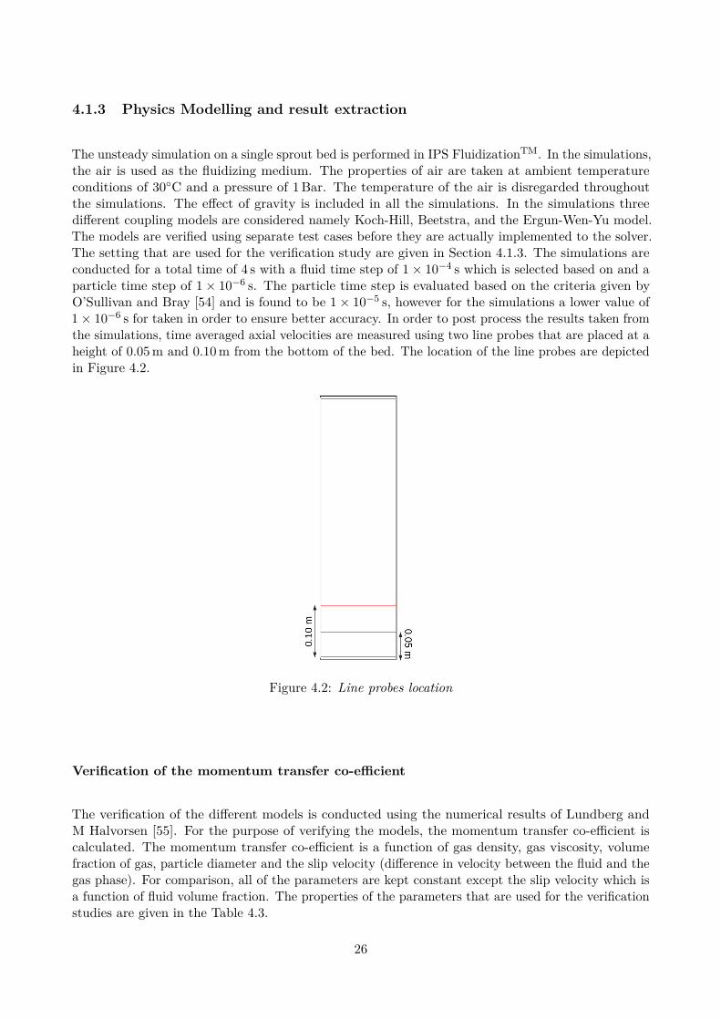
The unsteady simulation on a single sprout bed is performed in IPS FluidizationTM. In the simulations,the air is used as the fluidizing medium. The properties of air are taken at ambient temperatureconditions of 30◦C and a pressure of 1 Bar. The temperature of the air is disregarded throughoutthe simulations. The effect of gravity is included in all the simulations. In the simulations threedifferent coupling models are considered namely Koch-Hill, Beetstra, and the Ergun-Wen-Yu model.The models are verified using separate test cases before they are actually implemented to the solver.The setting that are used for the verification study are given in Section 4.1.3. The simulations areconducted for a total time of 4 s with a fluid time step of 1× 10−4 s which is selected based on and aparticle time step of 1× 10−6 s. The particle time step is evaluated based on the criteria given byO’Sullivan and Bray [54] and is found to be 1× 10−5 s, however for the simulations a lower value of1× 10−6 s for taken in order to ensure better accuracy. In order to post process the results taken fromthe simulations, time averaged axial velocities are measured using two line probes that are placed at aheight of 0.05 m and 0.10 m from the bottom of the bed. The location of the line probes are depictedin Figure 4.2.

Figure 4.2: Line probes location

Verification of the momentum transfer co-efficient

The verification of the different models is conducted using the numerical results of Lundberg andM Halvorsen [55]. For the purpose of verifying the models, the momentum transfer co-efficient iscalculated. The momentum transfer co-efficient is a function of gas density, gas viscosity, volumefraction of gas, particle diameter and the slip velocity (difference in velocity between the fluid and thegas phase). For comparison, all of the parameters are kept constant except the slip velocity which isa function of fluid volume fraction. The properties of the parameters that are used for the verificationstudies are given in the Table 4.3.

26

Table 4.3: Properties used in calculation of momentum transfer co-efficient for the verification study.

Diameter 154 µmGas Density 1.225 kg/m3

Gas viscosity 1.7894 ×10−5 kg/m.sSlip Velocity 0.133/εf

4.2 Heat transfer Simulation

In this Section 4.2, settings that are deployed to perform verification studies on the heat transfersolver are described. due to lack of experimental data only verification studies are performed.

4.2.1 Numerical settings used for heat transfer model verification

It is essential for the heat solver to be verified as this dictates the rate of evaporation from theliquid spray present over the particle. The implementation of the heat transfer models is verifiedby conducting single particle simulations in IPS FluidizationTM and comparing it with results froma 1D simulations carried out using a separate 1D model. The unsteady heat transfer simulation iscarried out using a single particle. In the simulations, the temperature of the particle is initiated to avalue of 273 K while the temperature of background fluid is varied from 283 K to 313 K in steps of10 K. The particle is fixed in space as the effect of gravity is neglected and the background fluid isconsidered stagnant. Water is used as the background fluid with all its properties taken at ambientconditions. The fluid time step is kept as 1× 10−4 s while the particle time step is kept as 1× 10−6 sec.The simulations are performed for a total time of 5 s. For results comparison, time evolution of thetemperature from both the IPS FluidizationTM and the 1D model are compared. After which the timeindependence of the heat solver is verified, by extending the same simulation in IPS FluidizationTM

with two more fluid steps (1e-4 s , 1e-6 s).

4.3 Spray Simulations

The most widely used apparatus in pharmaceutical and chemical industries for coating and drying ofpellets is a Wursted fluidized bed. In order to replicate the same conditions as in the industries, thesimulations are performed on the Wursted fluidized bed. For this purpose, the experimental studiesconducted by Liang et al. [36] on a Wursted fluidized bed is considered. The geometrical details ofthe setup used in the simulations taken from [36] are given in the Section 4.3.1. In the subsequentSection 4.3.2, details of the mesh and the boundary conditions used in the simulations are described.

4.3.1 Geometry of the Wurster Bed

The main components of the Wurster bed are the Wurster column, the spray nozzle and the distributorplate. The distributor plate, which is mainly used as an input for the fluidizing air is placed at thebottom of the bed and is divided into sections. The geometry of the simulation chamber used in thesimulations is given in Figure 4.3. The total height of the simulation chamber is 417 mm with thetop and bottom diameters as 250 mm and 100 mm respectively. The Wurster column is placed at aheight of 15 mm from the bottom of the distributor plate, the diameter of the Wurster column is50 mm and it has a height of 60 mm. The truncated conical section of the simulation chamber has a

27

height of 220 mm. The spray nozzle is placed at the bottom of the bed, it has an inner and outerdiameter of 12 mm and 5 mm respectively. The complete dimension of the bed is given in Table 4.4with the cross sectional view showing the dimensions given in Figure 4.4.

Figure 4.3: Schematic of the Wursted bed geometry representing different boundary regions.

28

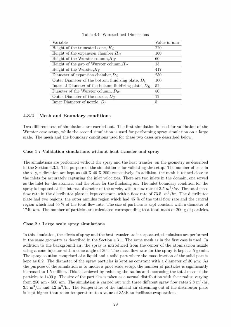
Table 4.4: Wursted bed Dimensions

Variable Value in mmHeight of the truncated cone, HC 220Height of the expansion chamber,HE 160Height of the Wurster column,HW 60Height of the gap of Wurster column,HP 15Height of the Wurster,HT 417Diameter of expansion chamber,DC 250Outer Diameter of the bottom fluidizing plate, DB 100Internal Diameter of the bottom fluidizing plate, DE 52Diamter of the Wurster column, DW 50Outer Diameter of the nozzle, DO 12Inner Diameter of nozzle, DI 5

4.3.2 Mesh and Boundary conditions

Two different sets of simulations are carried out. The first simulation is used for validation of theWurster case setup, while the second simulation is used for performing spray simulation on a largescale. The mesh and the boundary conditions used for these two cases are described below.

Case 1 : Validation simulations without heat transfer and spray

The simulations are performed without the spray and the heat transfer, on the geometry as describedin the Section 4.3.1. The purpose of the simulation is for validating the setup. The number of cells inthe x, y, z direction are kept as (40 X 40 X 200) respectively. In addition, the mesh is refined close tothe inlets for accurately capturing the inlet velocities. There are two inlets in the domain, one servedas the inlet for the atomizer and the other for the fluidizing air. The inlet boundary condition for thespray is imposed at the internal diameter of the nozzle, with a flow rate of 3.5 m3/hr. The total massflow rate in the distributor plate is kept constant, with a flow rate of 73.5 m3/hr. The distributorplate had two regions, the outer annulus region which had 45 % of the total flow rate and the centralregion which had 55 % of the total flow rate. The size of particles is kept constant with a diameter of1749 µm. The number of particles are calculated corresponding to a total mass of 200 g of particles.

Case 2 : Large scale spray simulations

In this simulation, the effects of spray and the heat transfer are incorporated, simulations are performedin the same geometry as described in the Section 4.3.1. The same mesh as in the first case is used. Inaddition to the background air, the spray is introduced from the center of the atomization nozzleusing a cone injector with a cone angle of 30◦. The mass flow rate for the spray is kept as 5 g/min.The spray solution comprised of a liquid and a solid part where the mass fraction of the solid part iskept as 0.2. The diameter of the spray particles is kept as constant with a diameter of 30 µm. Asthe purpose of the simulation is to model a pilot scale setup, the number of particles is significantlyincreased to 1.5 million. This is achieved by reducing the radius and increasing the total mass of theparticles to 1400 g. The size of the particles is taken as a normal distribution with their radius varyingfrom 250 µm - 500 µm. The simulation is carried out with three different spray flow rates 2.8 m3/hr,3.5 m3/hr and 4.2 m3/hr. The temperature of the ambient air streaming out of the distributor plateis kept higher than room temperature to a value of 353K to facilitate evaporation.

29

Figure 4.4: Sectional view of the Wurster bed along with the dimension.

4.3.3 Physics Modelling and result extraction

Similar to the previous Section 4.3.2, this is also categorized into two different cases. As some of thesettings are common to both the cases they are just described once.

Case 1 : Validation simulations without heat transfer and spray

The particle properties used in this case are given in the Table 4.5. The simulation is carried for atotal time of 21 s using the Ergun-Wen-Yu drag model. The model is taken so as to compare theresults taken from [56] where they had used the combination of Ergun-Wen-Yu drag model. The timestep for the particles and the fluid is kept as 5e-6 s and 1e-4 s respectively. The air is used as thefluidizing gas and its properties are taken at ambient conditions. The time averaged axial velocity ofthe particle is measured at a height of 90 mm for validation purpose.

30

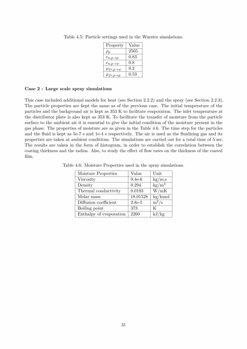
Table 4.5: Particle settings used in the Wurster simulations.

Property Valueρp 2505en,p→p 0.83en,p→w 0.8µfr,p→w 0.2µfr,p→p 0.53

Case 2 : Large scale spray simulations

This case included additional models for heat (see Section 2.2.2) and the spray (see Section 2.2.3).The particle properties are kept the same as of the previous case. The initial temperature of theparticles and the background air is kept as 353 K to facilitate evaporation. The inlet temperature atthe distributor plate is also kept as 353 K. To facilitate the transfer of moisture from the particlesurface to the ambient air it is essential to give the initial condition of the moisture present in thegas phase. The properties of moisture are as given in the Table 4.6. The time step for the particlesand the fluid is kept as 5e-7 s and 1e-4 s respectively. The air is used as the fluidizing gas and itsproperties are taken at ambient conditions. The simulations are carried out for a total time of 5 sec.The results are taken in the form of histogram, in order to establish the correlation between thecoating thickness and the radius. Also, to study the effect of flow rates on the thickness of the coatedfilm.

Table 4.6: Moisture Properties used in the spray simulations.

Moisture Properties Value UnitViscosity 9.4e-6 kg/m.sDensity 0.294 kg/m3

Thermal conductivity 0.0193 W/mKMolar mass 18.01528 kg/kmolDiffusion coefficient 2.8e-5 m2/sBoiling point 373 KEnthalpy of evaporation 2260 kJ/kg

31

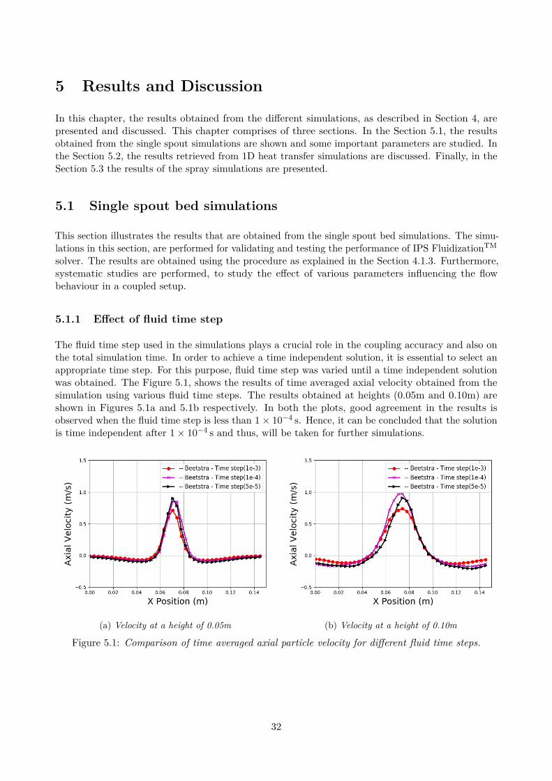
5 Results and Discussion

In this chapter, the results obtained from the different simulations, as described in Section 4, arepresented and discussed. This chapter comprises of three sections. In the Section 5.1, the resultsobtained from the single spout simulations are shown and some important parameters are studied. Inthe Section 5.2, the results retrieved from 1D heat transfer simulations are discussed. Finally, in theSection 5.3 the results of the spray simulations are presented.

5.1 Single spout bed simulations

This section illustrates the results that are obtained from the single spout bed simulations. The simu-lations in this section, are performed for validating and testing the performance of IPS FluidizationTM

solver. The results are obtained using the procedure as explained in the Section 4.1.3. Furthermore,systematic studies are performed, to study the effect of various parameters influencing the flowbehaviour in a coupled setup.

5.1.1 Effect of fluid time step

The fluid time step used in the simulations plays a crucial role in the coupling accuracy and also onthe total simulation time. In order to achieve a time independent solution, it is essential to select anappropriate time step. For this purpose, fluid time step was varied until a time independent solutionwas obtained. The Figure 5.1, shows the results of time averaged axial velocity obtained from thesimulation using various fluid time steps. The results obtained at heights (0.05m and 0.10m) areshown in Figures 5.1a and 5.1b respectively. In both the plots, good agreement in the results isobserved when the fluid time step is less than 1× 10−4 s. Hence, it can be concluded that the solutionis time independent after 1× 10−4 s and thus, will be taken for further simulations.

(a) Velocity at a height of 0.05m (b) Velocity at a height of 0.10m

Figure 5.1: Comparison of time averaged axial particle velocity for different fluid time steps.

32

5.1.2 Momentum-Models

In this section, the three different momentum exchange models, as given in Section 2.4.1 are compared.The models are verified using 1D models before they are tested in the solver using actual 2D spoutsimulations. This section is further split into two section. In the first subsection, the results obtainedfrom the verification studies for comparing momentum transfer coefficient is presented followed bythe validations studies in the subsequent section.

Verification of the Momentum transfer coefficient

The momentum transfer coefficient is calculated by varying the particle volume fraction. TheFigure 5.2, shows the comparison between the 1D models and the numerical results given in theliterature [55]. It is found that the momentum exchange coefficient increases with increasing particlevolume fraction. The 1D results obtained from the Koch-Hill model tends to under predict the valuesin comparison to numerical results from literature when the particle volume fraction is less than 0.4.Also, Koch-Hill model is found to give higher value of momentum exchange coefficient, at higherparticle volume fraction in comparison to Gidaspow model. Good agreement is observed, in case ofGidaspow model. However, Beetstra model couldn’t be verified due to unavailability of results inthe literature. All three models are further studied using 2D single spout simulations. The results ofwhich are discussed in subsequent section.

Figure 5.2: Comparison of Momentum transfer coefficients

33

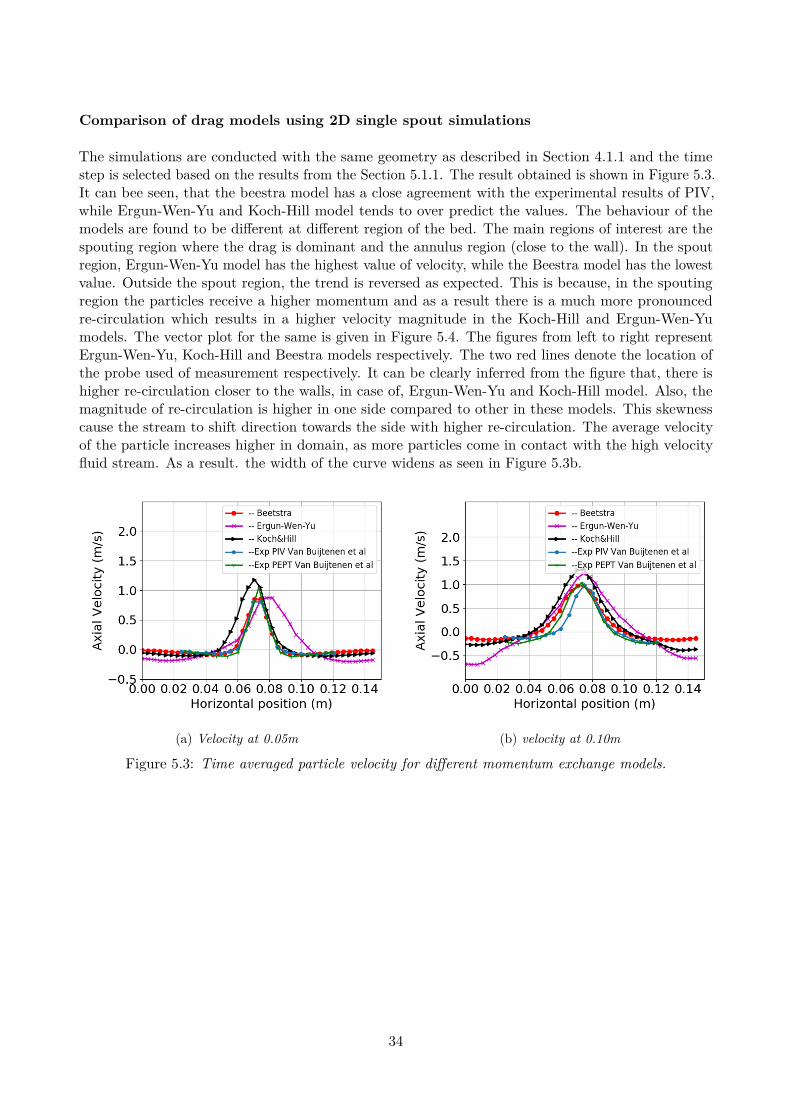
Comparison of drag models using 2D single spout simulations

The simulations are conducted with the same geometry as described in Section 4.1.1 and the timestep is selected based on the results from the Section 5.1.1. The result obtained is shown in Figure 5.3.It can bee seen, that the beestra model has a close agreement with the experimental results of PIV,while Ergun-Wen-Yu and Koch-Hill model tends to over predict the values. The behaviour of themodels are found to be different at different region of the bed. The main regions of interest are thespouting region where the drag is dominant and the annulus region (close to the wall). In the spoutregion, Ergun-Wen-Yu model has the highest value of velocity, while the Beestra model has the lowestvalue. Outside the spout region, the trend is reversed as expected. This is because, in the spoutingregion the particles receive a higher momentum and as a result there is a much more pronouncedre-circulation which results in a higher velocity magnitude in the Koch-Hill and Ergun-Wen-Yumodels. The vector plot for the same is given in Figure 5.4. The figures from left to right representErgun-Wen-Yu, Koch-Hill and Beestra models respectively. The two red lines denote the location ofthe probe used of measurement respectively. It can be clearly inferred from the figure that, there ishigher re-circulation closer to the walls, in case of, Ergun-Wen-Yu and Koch-Hill model. Also, themagnitude of re-circulation is higher in one side compared to other in these models. This skewnesscause the stream to shift direction towards the side with higher re-circulation. The average velocityof the particle increases higher in domain, as more particles come in contact with the high velocityfluid stream. As a result. the width of the curve widens as seen in Figure 5.3b.

(a) Velocity at 0.05m (b) velocity at 0.10m

Figure 5.3: Time averaged particle velocity for different momentum exchange models.

34

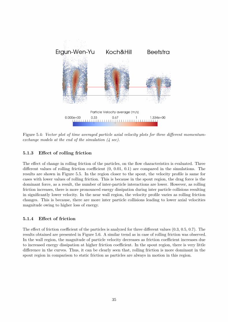
Figure 5.4: Vector plot of time averaged particle axial velocity plots for three different momentum-exchange models at the end of the simulation (4 sec).

5.1.3 Effect of rolling friction

The effect of change in rolling friction of the particles, on the flow characteristics is evaluated. Threedifferent values of rolling friction coefficient (0, 0.01, 0.1) are compared in the simulations. Theresults are shown in Figure 5.5. In the region closer to the spout, the velocity profile is same forcases with lower values of rolling friction. This is because in the spout region, the drag force is thedominant force, as a result, the number of inter-particle interactions are lower. However, as rollingfriction increases, there is more pronounced energy dissipation during inter particle collisions resultingin significantly lower velocity. In the near wall region, the velocity profile varies as rolling frictionchanges. This is because, there are more inter particle collisions leading to lower axial velocitiesmagnitude owing to higher loss of energy.

5.1.4 Effect of friction

The effect of friction coefficient of the particles is analyzed for three different values (0.3, 0.5, 0.7). Theresults obtained are presented in Figure 5.6. A similar trend as in case of rolling friction was observed.In the wall region, the magnitude of particle velocity decreases as friction coefficient increases dueto increased energy dissipation at higher friction coefficient. In the spout region, there is very littledifference in the curves. Thus, it can be clearly seen that, rolling friction is more dominant in thespout region in comparison to static friction as particles are always in motion in this region.

35

(a) Velocity at 0.05m (b) velocity at 0.10m

Figure 5.5: Time averaged particle velocity for different values of rolling friction

(a) Velocity at 0.05m (b) velocity at 0.10m

Figure 5.6: Time averaged particle velocity for different friction-coefficient

5.2 1D heat transfer simulations

In this section, the result obtained from the heat transfer simulations carried out using IPSfluidizationTM and the 1D model are presented. In Figure 5.7, time evolution of temperatureare compared. In all the cases, the temperature of the particle increases until it reaches the stagnantair conditions. Good agreement in the results are observed with the 1D simulation which verifiesthe implementation of the heat transfer model. In addition to verifying the heat transfer model inthe solver IPS fluidizationTM, the fluid time step is also varied to check the accuracy of the solver.The results can be seen in Figure 5.8. Although, all three time step gives the same time evolution oftemperature, this may not give an exact representation of the time step that is required to obtain atime independent solution as the background air is considered stagnant in the current simulation.However, it verifies that the solver is stable even for longer time steps in simple cases. The validationof the heat transfer cannot be performed due to difficulty in finding an ideal data from the literature.

36

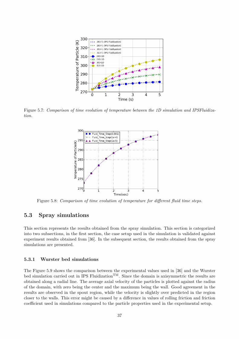
Figure 5.7: Comparison of time evolution of temperature between the 1D simulation and IPSFluidiza-tion.

Figure 5.8: Comparison of time evolution of temperature for different fluid time steps.

5.3 Spray simulations

This section represents the results obtained from the spray simulation. This section is categorizedinto two subsections, in the first section, the case setup used in the simulation is validated againstexperiment results obtained from [36]. In the subsequent section, the results obtained from the spraysimulations are presented.

5.3.1 Wurster bed simulations

The Figure 5.9 shows the comparison between the experimental values used in [36] and the Wursterbed simulation carried out in IPS FluidizationTM. Since the domain is axisymmetric the results areobtained along a radial line. The average axial velocity of the particles is plotted against the radiusof the domain, with zero being the center and the maximum being the wall. Good agreement in theresults are observed in the spout region, while the velocity is slightly over predicted in the regioncloser to the walls. This error might be caused by a difference in values of rolling friction and frictioncoefficient used in simulations compared to the particle properties used in the experimental setup.

37

Figure 5.9: Comparison of axial velocity from simulation with the experimental study of Li Liang etal.

5.3.2 Wurster bed spray simulations

In this section, the results obtained from spray simulations are presented. Figure 5.10 shows thehistogram plot of particles with a given coating thickness for various nozzle flow rates. As observedfrom Figure 5.10a - 5.10d, the number of particles with a coating thickness, increases significantlyas time progresses. This is because more particles come in contact with the spray over time. Thisis clearly shown in Figure 5.11, where the time evolution of the accumulated mass is shown for asingle case. The number of particles having thinner coating is higher for higher flow rates. This isbecause at higher flow rates, more particles come in contact with spray. However, at higher flow rates,the particles are exposed to larger drag force and hence, they are faster transported from the sprayinjection zone.

5.3.3 Correlation between particle radius and thickness of the film

In order to study the correlation between the particle radius and the thickness of the coating, marginalplots are plotted. A marginal plot allows to study the relationship between two numeric variables.The marginal charts, at the top and at the right, shows the distribution of the two variables using thedensity plots, while the central chart displays their correlation. In the Figure 5.12, the correlationbetween particle radius and thickness of deposited film is plotted. The plot at the top, shows thedistribution of particles with a given radius having coating, i.e. that has been hit by at least onespray droplet. While the plot on the right side, displays the distribution of accumulated droplet mass,independent of the radius. In the center, the correlation plot is shown. A total of 43992 particles havebeen hit by the spray out of 1.4M particles after a time of 5s. The density plot at the top and rightshows only the particles that has been hit by the spray. From the top, density plot, it can be inferredthat, there are more number of bigger particles having coating in comparison to smaller particles.This is because bigger particles have higher surface area and hence probability of them have collisionwith spray parcels is higher. Also bigger particles have higher mass and stay close to the spray regiondue to reduced drag per mass, thus creating a shielding effecting for smaller particles. From the right,density plot, it can be seen that, there are more of particles having thinner film in comparison to

38

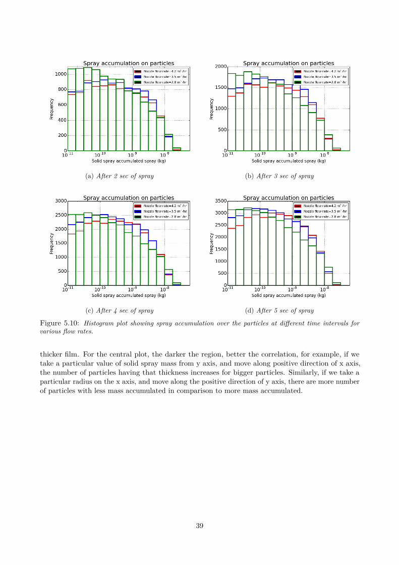
(a) After 2 sec of spray (b) After 3 sec of spray

(c) After 4 sec of spray (d) After 5 sec of spray

Figure 5.10: Histogram plot showing spray accumulation over the particles at different time intervals forvarious flow rates.

thicker film. For the central plot, the darker the region, better the correlation, for example, if wetake a particular value of solid spray mass from y axis, and move along positive direction of x axis,the number of particles having that thickness increases for bigger particles. Similarly, if we take aparticular radius on the x axis, and move along the positive direction of y axis, there are more numberof particles with less mass accumulated in comparison to more mass accumulated.

39

(a) Spray accumulated for flow rate 3.5m3/hr (b) Spray accumulated for flow rate 4.2m3/hr

Figure 5.11: Spray accumulation over time with varying flow rates

Figure 5.12: Plot showing correlation between the radii of the particle and the spray accumulated forNozzle Flow rate = 4.2m3/hr

40

6 Conclusion

The main objective of this thesis has been to simulate and study the pellet coating process, as well as,to test the scalability of the solver in carrying out computational intensive simulations with morethan a million particles with the spray treated in a Lagrangian manner.

The study was carried out in three parts, in the initial phase, the single spout simulations were carriedout using the solver IPS FluidizationTM developed at FCC with an aim to validate the coupled solver.The solver was found to be time independent after a fluid time step of 0.1 ms for such simulations.Three different momentum exchange models were compared against experimental data available inthe open literature. The Beetstra momentum model, was found to produce accurate results andshowed close agreement with the PIV experimental results from [14]. Further, the effect of rollingfriction and friction coefficient of particle were evaluated. It was found that, as rolling friction wasincreased, the loss of energy during each interparticle collisions was also significantly higher, resultingin reduced velocity magnitude.

The heat transfer model, which was added to the solver (IPS FluidizationTM) by FCC was verified inthis thesis by using 1D models. The simulations conducted using the solver showed identical matchwith the 1D models and thus verifying the heat transfer model in the solver.

In order to carry out spray simulations, the setup used in [36] was used. The results were obtainedin the form of time averaged axial velocity thus validating the setup. The plots showed goodcorrespondence with the numerical values available in the literature. The number of particles inthe spray simulations was scaled to be more than a million. The results were taken in the form ofhistogram. The general trend showed, as expected, that at lower nozzle flow rates, there were morenumber of particles having a thicker coating. While, at higher flow rates, there were more number ofparticles having a thinner coating. The results also showed that there were higher numbers of of largerparticles having coating in comparison to smaller particles. This is because the bigger particles havehigher surface area and also they tend to stay closer to the nozzle region due to their higher mass andhence create a shielding effect for the smaller particles. The results also proved the effectiveness ofthe solver IPS FluidizationTM in carrying out full physics large scale coating simulations.

41

References

[1] G. L. Matheson, W. Herbst, and P. Hol, Ind. Eng. Chem. 1949, p. 1099.[2] K. B. Mathur and P. E. Gishler, A study of the application of the spouted bed technique to

wheat drying, Journal of Applied Chemistry 5, no. 11 1955, 624–636, 1955. doi: 10.1002/jctb.5010051106. eprint: https://onlinelibrary.wiley.com/doi/pdf/10.1002/jctb.5010051106. [Online]. Available: https://onlinelibrary.wiley.com/doi/abs/10.1002/jctb.5010051106.

[3] V. S. Sutkar, N. G. Deen, and J. Kuipers, Spout fluidized beds: Recent advances in experimentaland numerical studies, Chemical Engineering Science 86 2013, 124–136, 2013, 5th InternationalGranulation Workshop, issn: 0009-2509. doi: https://doi.org/10.1016/j.ces.2012.06 . 022. [Online]. Available: http : / / www . sciencedirect . com / science / article / pii /S0009250912003715.

[4] A. Nagarkatti and A. Chatterjee, Pressure and flow characteristics of a gas phase spout-fluid bedand the minimum spout-fluid condition, The Canadian Journal of Chemical Engineering 52, no. 21974, 185–195, 1974. doi: 10.1002/cjce.5450520209. eprint: https://onlinelibrary.wiley.com/doi/pdf/10.1002/cjce.5450520209. [Online]. Available: https://onlinelibrary.wiley.com/doi/abs/10.1002/cjce.5450520209.

[5] Chatterjee and Asok, Spout-fluid bed technique, Industrial & Engineering Chemistry ProcessDesign and Development 9, no. 2 1970, 340–341, 1970. doi: 10.1021/i260034a032. eprint:https://doi.org/10.1021/i260034a032. [Online]. Available: https://doi.org/10.1021/i260034a032.

[6] M. L. Passos, A. S. Mujumdar, G. Vijaya, and V. G. Raghavan, Spouted and spout-fluidizedbeds for gram drying, Drying Technology 7, no. 4 1989, 663–696, 1989. doi: 10 . 1080 /07373938908916621. eprint: https://doi.org/10.1080/07373938908916621. [Online]. Avail-able: https://doi.org/10.1080/07373938908916621.

[7] Spouted and Spout-Fluid Beds: Fundamentals and Applications. Cambridge University Press,2010. doi: 10.1017/CBO9780511777936.

[8] W. de Oliveira, J. Freire, and J. Coury, Analysis of particle coating by spouted bed process,International Journal of Pharmaceutics 158, no. 1 1997, 1–9, 1997, issn: 0378-5173. doi:https://doi.org/10.1016/S0378- 5173(97)00181- 6. [Online]. Available: http://www.sciencedirect.com/science/article/pii/S0378517397001816.

[9] R. Cunha, K. G Maialle, and F. Menegalli, Evaluation of the drying process in spouted bedand spout fluidized bed of xanthan gum: Focus on product quality, Powder Technology 107Feb. 2000, 234–242, Feb. 2000. doi: 10.1016/S0032-5910(99)00197-7.

[10] W. Ludwig, R. Szafran, A. Kmiec, and J. Dziak, Dry powder coating in a modified wursterapparatus, Procedia Engineering 42 2012, 437–446, 2012, CHISA 2012, issn: 1877-7058. doi:https://doi.org/10.1016/j.proeng.2012.07.435. [Online]. Available: http://www.sciencedirect.com/science/article/pii/S1877705812028354.

[11] J. Pritchett, T. Blake, and S. Garg, A numerical model of gas fluidized beds, AIChE Symp Ser74 Jan. 1978, 134–148, Jan. 1978.

[12] Y. Tsuji, T. Kawaguchi, and T. Tanaka, Discrete particle simulation of two-dimensional fluidizedbed, Powder Technology 77, no. 1 1993, 79–87, 1993, issn: 0032-5910. doi: https://doi.org/10.1016/0032-5910(93)85010-7. [Online]. Available: http://www.sciencedirect.com/science/article/pii/0032591093850107.

[13] P. Cundall and O. Strack, A discrete numerical model for granular assemblies, English (US),Geotechnique 29, no. 1 Mar. 1979, 47–65, Mar. 1979, issn: 0016-8505. doi: 10.1680/geot.1979.29.1.47.

42

[14] M. S. van Buijtenen, W.-J. van Dijk, N. G. Deen, J. Kuipers, T. Leadbeater, and D. Parker,Numerical and experimental study on multiple-spout fluidized beds, Chemical EngineeringScience 66, no. 11 2011, 2368–2376, 2011, issn: 0009-2509. doi: https://doi.org/10.1016/j.ces.2011.02.055. [Online]. Available: http://www.sciencedirect.com/science/article/pii/S0009250911001564.

[15] R. Chopra, G. Alderborn, J. M. Newton, and F. Podczeck, The influence of film coating onpellet properties, Pharmaceutical Development and Technology 7, no. 1 2002, 59–68, 2002.doi: 10.1081/PDT-120002231. eprint: https://doi.org/10.1081/PDT-120002231. [Online].Available: https://doi.org/10.1081/PDT-120002231.

[16] K. Jono, H. Ichikawa, M. Miyamoto, and Y. Fukumori, A review of particulate design forpharmaceutical powders and their production by spouted bed coating, Powder Technology113, no. 3 2000, 269–277, 2000, Neptis Symposium on Fluidization- Present and Future, issn:0032-5910. doi: https://doi.org/10.1016/S0032-5910(00)00310-7. [Online]. Available:http://www.sciencedirect.com/science/article/pii/S0032591000003107.

[17] A. V. Patil, E. Peters, T. Kolkman, and J. Kuipers, Modeling bubble heat transfer in gassolid fluidized beds using dem, Chemical Engineering Science 105 2014, 121–131, 2014, issn:0009-2509. doi: https : / / doi . org / 10 . 1016 / j . ces . 2013 . 11 . 001. [Online]. Available:http://www.sciencedirect.com/science/article/pii/S0009250913007306.

[18] A. Patil, E. Peters, and J. Kuipers, Computational study of particle temperature in a bubblingspout fluidized bed with hot gas injection, Powder Technology 284 2015, 475–485, 2015, issn:0032-5910. doi: https://doi.org/10.1016/j.powtec.2015.07.014. [Online]. Available:http://www.sciencedirect.com/science/article/pii/S003259101500546X.

[19] T. Tsory, N. Ben-Jacob, T. Brosh, and A. Levy, Thermal dem–cfd modeling and simulationof heat transfer through packed bed, Powder Technology 244 2013, 52–60, 2013, issn: 0032-5910. doi: https://doi.org/10.1016/j.powtec.2013.04.013. [Online]. Available: http://www.sciencedirect.com/science/article/pii/S0032591013002702.

[20] H. Wu, N. Gui, X. Yang, J. Tu, and S. Jiang, Numerical simulation of heat transfer in packedpebble beds: Cfd-dem coupled with particle thermal radiation, International Journal of Heatand Mass Transfer 110 2017, 393–405, 2017, issn: 0017-9310. doi: https://doi.org/10.1016/j.ijheatmasstransfer.2017.03.035. [Online]. Available: http://www.sciencedirect.com/science/article/pii/S0017931016331386.

[21] M. Askarishahi, M.-S. Salehi, and S. Radl, Full-physics simulations of spray-particle interactionin a bubbling fluidized bed, AIChE Journal 63, no. 7 2017, 2569–2587, 2017. doi: 10.1002/aic.15616. eprint: https://onlinelibrary.wiley.com/doi/pdf/10.1002/aic.15616. [Online].Available: https://onlinelibrary.wiley.com/doi/abs/10.1002/aic.15616.

[22] V. S. Sutkar, N. G. Deen, A. V. Patil, V. Salikov, S. Antonyuk, S. Heinrich, and J. Kuipers,Cfd dem model for coupled heat and mass transfer in a spout fluidized bed with liquidinjection, Chemical Engineering Journal 288 2016, 185–197, 2016, issn: 1385-8947. doi: https://doi.org/10.1016/j.cej.2015.11.044. [Online]. Available: http://www.sciencedirect.com/science/article/pii/S1385894715015879.

[23] W. I. Kariuki, B. Freireich, R. M. Smith, M. Rhodes, and K. P. Hapgood, Distribution nucleation:Quantifying liquid distribution on the particle surface using the dimensionless particle coatingnumber, Chemical Engineering Science 92 2013, 134–145, 2013, issn: 0009-2509. doi: https://doi.org/10.1016/j.ces.2013.01.010. [Online]. Available: http://www.sciencedirect.com/science/article/pii/S0009250913000134.

[24] A.Mark and B. van Wachem, Derivation and validation of a novel implicit second-order accurateimmersed boundary method, Journal of Computational Physics 227, no. 13 2008, 6660–6680,2008.

43

[25] A.Mark, R.Rundqvist, and F.Edelvik, Comparison between different immersed boundary condi-tions for simulation of complex fluid flows, Journal of Fluid Dynamics & Materials Processing7, no. 3 2011, 241–258, 2011.

[26] A. Mark, E. Svenning, R. Rundqvist, et al., Microstructure simulation of early paper formingusing immersed boundary methods, Tappi Journal 10, no. 11 2011, 23–30, 2011.

[27] T. Johnson, P. Röyttä, A. Mark, and F. Edelvik, Simulation of the spherical orientationprobability distribution of paper fibers in an entire suspension using immersed boundarymethods, Journal of Non-Newtonian Fluid Mechanics, no. 1 2016, 2016.

[28] A. Mark, B. Andersson, S. Tafuri, K. Engström, H. Söröd, F. Edelvik, and J. Carlson, Simulationof electrostatic rotary bell spray painting in automotive paint shops, Atomization and Sprays23, no. 1 2013, 25–45, 2013.

[29] F. Edelvik, A. Mark, N. Karlsson, T. Johnson, and J. S. Carlson, “Math-based algorithms andsoftware for virtual product realization implemented in automotive paint shops”, Math for theDigital factory. Springer Verlag, 2017, pp. 231–251.

[30] A. Mark, R. Bohlin, D. Segerdahl, F. Edelvik, and J. Carlson, Optimisation of robotised sealingstations in paint shops by process simulation and automatic path planning, International Journalof Manufacturing Research 9, no. 1 2014, 4–26, 2014.

[31] S. Ingelsten, A. Mark, and F. Edelvik, A lagrangian-eulerian framework for simulation oftransient viscoelastic fluid flow, Journal of Non-Newtonian Fluid Mechanics 266 2019, 20–32,2019, issn: 0377-0257. doi: https://doi.org/10.1016/j.jnnfm.2019.02.005. [Online].Available: http://www.sciencedirect.com/science/article/pii/S037702571830137X.

[32] J. Göhl, K. Markstedt, A. Mark, K. Håkansson, P. Gatenholm, and F. Edelvik, Simulations of3d bioprinting: Predicting bioprintability of nanofibrillar inks, Biofabrication 10, no. 3 2018,034105, 2018. doi: 10.1088/1758-5090/aac872.

[33] J.Göhl, A. Mark, S. Sasic, and F. Edelvik, An immersed boundary based dynamic contactangle framework for handling complex surfaces of mixed wettabilities, International Journal ofMultiphase Flow 109 2018, 164–177, 2018.

[34] D. Jajcevic, E. Siegmann, C. Radeke, and J. G. Khinast, Large-scale cfd–dem simulationsof fluidized granular systems, Chemical Engineering Science 98 2013, 298–310, 2013, issn:0009-2509. doi: https : / / doi . org / 10 . 1016 / j . ces . 2013 . 05 . 014. [Online]. Available:http://www.sciencedirect.com/science/article/pii/S000925091300345X.

[35] T. Tang, Y. He, T. Tai, and D. Wen, Dem numerical investigation of wet particle flow behaviorsin multiple-spout fluidized beds, Chemical Engineering Science 172 2017, 79–99, 2017, issn:0009-2509. doi: https : / / doi . org / 10 . 1016 / j . ces . 2017 . 06 . 025. [Online]. Available:http://www.sciencedirect.com/science/article/pii/S0009250917304153.

[36] L. Liang, R. Anders, I. Andy, J. Mats, R. Johan, von Corswant Christian, Folestad, andStaffan, Pept study of particle cycle and residence time distributions in a wurster fluid bed,AIChE Journal 61, no. 3 2015, 756–768, 2015. doi: 10.1002/aic.14692. eprint: https://aiche.onlinelibrary.wiley.com/doi/pdf/10.1002/aic.14692. [Online]. Available:https://aiche.onlinelibrary.wiley.com/doi/abs/10.1002/aic.14692.

[37] H. Versteeg and W. Malalasekera, An Introduction to Computational Fluid Dynamics: TheFinite Volume Approach. Longman Scientific & Technical, 1995, isbn: 9780582218840. [Online].Available: https://books.google.se/books?id=7UynjgEACAAJ.

[38] M. Syamlal and D. Gidaspow, Hydrodynamics of fluidization: Prediction of wall to bed heat trans-fer coefficients, AIChE Journal 31, no. 1 1985, 127–135, 1985. doi: 10.1002/aic.690310115.eprint: https://aiche.onlinelibrary.wiley.com/doi/pdf/10.1002/aic.690310115.[Online]. Available: https://aiche.onlinelibrary.wiley.com/doi/abs/10.1002/aic.690310115.

44

[39] M. S. van Buijtenen, N. G. Deen, S. Heinrich, S. Antonyuk, and J. A. M. Kuipers, A discreteelement study of wet particle particle interaction during granulation in a spout fluidized bed,The Canadian Journal of Chemical Engineering 87, no. 2 2009, 308–317, 2009. doi: 10.1002/cjce.20144. eprint: https://onlinelibrary.wiley.com/doi/pdf/10.1002/cjce.20144.[Online]. Available: https://onlinelibrary.wiley.com/doi/abs/10.1002/cjce.20144.

[40] C. Thornton, S. J. Cummins, and P. W. Cleary, An investigation of the comparative behaviour ofalternative contact force models during elastic collisions, Powder Technology 210, no. 3 2011, 189–197, 2011, issn: 0032-5910. doi: https://doi.org/10.1016/j.powtec.2011.01.013. [Online].Available: http://www.sciencedirect.com/science/article/pii/S0032591011000325.

[41] K. L. Johnson, Contact Mechanics. Cambridge University Press, 1985. doi: 10.1017/CBO9781139171731.[42] R. D. Mindlin, Compliance of elastic bodies in contact, J. Appl. Mech., ASME 16 1949, 259–268,

1949. [Online]. Available: https://ci.nii.ac.jp/naid/10013415139/en/.[43] J. Ai, J.-F. Chen, J. M. Rotter, and J. Y. Ooi, Assessment of rolling resistance models in

discrete element simulations, Powder Technology 206, no. 3 2011, 269–282, 2011, issn: 0032-5910. doi: https://doi.org/10.1016/j.powtec.2010.09.030. [Online]. Available: http://www.sciencedirect.com/science/article/pii/S0032591010005164.

[44] D. Gunn, Transfer of heat or mass to particles in fixed and fluidised beds, InternationalJournal of Heat and Mass Transfer 21, no. 4 1978, 467–476, 1978, issn: 0017-9310. doi:https://doi.org/10.1016/0017- 9310(78)90080- 7. [Online]. Available: http://www.sciencedirect.com/science/article/pii/0017931078900807.

[45] S. Ergun, Fluid flow through packed columns, Fluid Flow Through Packed Columns 1952, 89–94,1952, cited By 14.

[46] C. Wen and Y. Yu 1966, 100–111, 1966, cited By 1.[47] R. J. Hill, D. L. Koch, and A. J. C. Ladd, The first effects of fluid inertia on flows in ordered

and random arrays of spheres, Journal of Fluid Mechanics 448 2001, 213–241, 2001. doi:10.1017/S0022112001005948.

[48] R. Beetstra, M. A. van der Hoef, and J. A. M. Kuipers, Drag force of intermediate reynoldsnumber flow past mono- and bidisperse arrays of spheres, AIChE Journal 53, no. 2 2007,489–501, 2007. doi: 10.1002/aic.11065. eprint: https://onlinelibrary.wiley.com/doi/pdf/10.1002/aic.11065. [Online]. Available: https://onlinelibrary.wiley.com/doi/abs/10.1002/aic.11065.

[49] C. Romero Luna, I. Avila, L. R. CARROCCI, and G. Arce, A cfd assessment of drag modelsperformance on gas-solid flow hydrodynamics in a fluidized bed Feb. 2015, 5202–5218, Feb. 2015.doi: 10.5151/chemeng-cobeq2014-0017-27527-160466.

[50] J. P. V. Doormaal and G. D. Raithby, Enhancements of the simple method for predictingincompressible fluid flows, Numerical Heat Transfer 7, no. 2 1984, 147–163, 1984. doi: 10.1080/01495728408961817. eprint: https://doi.org/10.1080/01495728408961817. [Online].Available: https://doi.org/10.1080/01495728408961817.

[51] C. RHIE and W. CHOW, Numerical study of the turbulent flow past an airfoil with trailingedge separation, AIAA Journal 21, no. 11 1983, 1525–1532, 1983. doi: 10.2514/3.8284. eprint:https://doi.org/10.2514/3.8284. [Online]. Available: https://doi.org/10.2514/3.8284.

[52] D. Kafui, S. Johnson, C. Thornton, and J. Seville, Parallelization of a lagrangian–euleriandem/cfd code for application to fluidized beds, Powder Technology 207, no. 1 2011, 270–278,2011, issn: 0032-5910. doi: https://doi.org/10.1016/j.powtec.2010.11.008. [Online].Available: http://www.sciencedirect.com/science/article/pii/S0032591010005887.

[53] C. A. Radeke, B. J. Glasser, and J. G. Khinast, Large-scale powder mixer simulations usingmassively parallel gpuarchitectures, Chemical Engineering Science 65, no. 24 2010, 6435–6442,2010, issn: 0009-2509. doi: https://doi.org/10.1016/j.ces.2010.09.035. [Online].Available: http://www.sciencedirect.com/science/article/pii/S0009250910005737.

45

[54] C. O’Sullivan and J. D. Bray, Selecting a suitable time step for discrete element simulationsthat use the central difference time integration scheme, Engineering Computations 21, no. 2/3/42004, 278–303, 2004. doi: 10.1108/02644400410519794.

[55] J. Lundberg and B. M Halvorsen, A review of some existing drag models describing the interactionbetween phases in a bubbling fluidized bed, Proc. Proc. 49th Scand. Conf. Simulation andModeling Jan. 2008, Jan. 2008.

[56] L. Li, J. Remmelgas, B. G. van Wachem, C. von Corswant, M. Johansson, S. Folestad, andA. Rasmuson, Residence time distributions of different size particles in the spray zone of awurster fluid bed studied using dem-cfd, Powder Technology 280 2015, 124–134, 2015, issn:0032-5910. doi: https://doi.org/10.1016/j.powtec.2015.04.031. [Online]. Available:http://www.sciencedirect.com/science/article/pii/S0032591015003058.

[57] S. Al-Arkawazi, Modeling the heat transfer between fluid-granular medium, Applied ThermalEngineering 128 2018, 696–705, 2018, issn: 1359-4311. doi: https://doi.org/10.1016/j.applthermaleng.2017.09.064. [Online]. Available: http://www.sciencedirect.com/science/article/pii/S1359431117344307.

[58] D. Gunn, Transfer of heat or mass to particles in fixed and fluidised beds, Int. J. Heat MassTransfer 21 Apr. 1978, 467–476, Apr. 1978. doi: 10.1016/0017-9310(78)90080-7.

[59] R. Kolakaluri, “Direct numerical simulations and analytical modeling of granular filtration”,2015.

[60] R. J. Hill, D. L. Koch, and A. J. C. Ladd, Moderate-reynolds-number flows in ordered andrandom arrays of spheres, Journal of Fluid Mechanics 448 2001, 243–278, 2001. doi: 10.1017/S0022112001005936.

[61] T. Mikami, H. Kamiya, and M. Horio, Numerical simulation of cohesive powder behaviorin a fluidized bed, Chemical Engineering Science 53, no. 10 1998, 1927–1940, 1998, issn:0009-2509. doi: https://doi.org/10.1016/S0009-2509(97)00325-4. [Online]. Available:http://www.sciencedirect.com/science/article/pii/S0009250997003254.

[62] G. H. Findenegg, J. n. israelachvili: Intermolecular and surface forces (with applications tocolloidal and biological systems). academic press, london, orlando, san diego, new york, toronto,montreal, sydney, tokyo 1985. 296 seiten, preis: $ 65.00. Berichte der Bunsengesellschaft fürphysikalische Chemie 90, no. 12 1986, 1241–1242, 1986. doi: 10.1002/bbpc.19860901226.eprint: https://onlinelibrary.wiley.com/doi/pdf/10.1002/bbpc.19860901226. [Online].Available: https://onlinelibrary.wiley.com/doi/abs/10.1002/bbpc.19860901226.

[63] R. B. Bird, Transport phenomena 1960, 1960.[64] B. Adam M .J Edmondson, Forces between particles in continuous and discrete liquid media,

Tribology in Particulate technology 1987, 1987.[65] G. Lian, M. J. Adams, and C. Thornton, Elastohydrodynamic collisions of solid spheres, Journal

of Fluid Mechanics 311 1996, 141–152, 1996. doi: 10.1017/S0022112096002534.[66] C. Song, D. Liu, J. Ma, and X. Chen, Cfd-dem simulation of flow pattern and particle velocity

in a fluidized bed with wet particles, Powder Technology 314 2017, 346–354, 2017, SpecialIssue on Simulation and Modelling of Particulate Systems, issn: 0032-5910. doi: https://doi.org/10.1016/j.powtec.2016.10.044. [Online]. Available: http://www.sciencedirect.com/science/article/pii/S0032591016307264.

[67] T. B. Anderson and R. Jackson, Fluid mechanical description of fluidized beds. equations ofmotion, Industrial & Engineering Chemistry Fundamentals 6, no. 4 1967, 527–539, 1967. doi:10.1021/i160024a007. eprint: https://doi.org/10.1021/i160024a007. [Online]. Available:https://doi.org/10.1021/i160024a007.

[68] J. R. Grace, Multiphase flow and fluidization: Continuum and kinetic theory descriptions by d.gidaspow, 1994, 467 + xx pages, academic press, san diego, ca, isbn 0-12-282470-9. price: Us$69.50, The Canadian Journal of Chemical Engineering 73, no. 5 1995, 784–784, 1995. doi:

46

10.1002/cjce.5450730523. eprint: https://onlinelibrary.wiley.com/doi/pdf/10.1002/cjce.5450730523. [Online]. Available: https://onlinelibrary.wiley.com/doi/abs/10.1002/cjce.5450730523.

[69] B. Crüger, V. Salikov, S. Heinrich, S. Antonyuk, V. Sutkar, N. Deen, and J. Kuipers, Coefficientof restitution for particles impacting on wet surfaces: An improved experimental approach,Particuology 25 2016, 1–9, 2016, issn: 1674-2001. doi: https://doi.org/10.1016/j.partic.2015.04.002. [Online]. Available: http://www.sciencedirect.com/science/article/pii/S1674200115001157.

[70] T. Müller and K. Huang, Influence of the liquid film thickness on the coefficient of restitutionfor wet particles, Phys. Rev. E 93 4 2016, 042904, 4 2016. doi: 10.1103/PhysRevE.93.042904.[Online]. Available: https://link.aps.org/doi/10.1103/PhysRevE.93.042904.

[71] T. Kawaguchi, M. Sakamoto, T. Tanaka, and Y. Tsuji, Quasi-three-dimensional numericalsimulation of spouted beds in cylinder, Powder Technology 109, no. 1 2000, 3–12, 2000, issn:0032-5910. doi: https://doi.org/10.1016/S0032-5910(99)00222-3. [Online]. Available:http://www.sciencedirect.com/science/article/pii/S0032591099002223.

[72] C. Thornton and C. Randall, Applications of theoretical contact mechanics to solid particlesystem simulation, Micromechanics of Granular Materials, Satake and Jenkins (eds) 20 Jan.1988, 133–142, Jan. 1988. doi: 10.1016/B978-0-444-70523-5.50023-0.

[73] C. M. Hrenya and J. L. Sinclair, Effects of particle-phase turbulence in gas-solid flows, AIChEJournal 43, no. 4 1997, 853–869, 1997. doi: 10.1002/aic.690430402. eprint: https://aiche.onlinelibrary.wiley.com/doi/pdf/10.1002/aic.690430402. [Online]. Available:https://aiche.onlinelibrary.wiley.com/doi/abs/10.1002/aic.690430402.

[74] M. R. Maxey and J. J. Riley, Equation of motion for a small rigid sphere in a nonuniformflow, The Physics of Fluids 26, no. 4 1983, 883–889, 1983. doi: 10.1063/1.864230. eprint:https://aip.scitation.org/doi/pdf/10.1063/1.86423. [Online]. Available: https://aip.scitation.org/doi/abs/10.1063/1.86423.

[75] C. T. Crowe, J. D. Schwarzkopf, and M. S. andYutaka Tsuji, Multiphase Flows with Dropletsand Particles, The Science of Microfabrication. CRC Press, 2011.

[76] E. Teunou and D. Poncelet, Batch and continuous fluid bed coating – review and state ofthe art, Journal of Food Engineering 53, no. 4 2002, 325–340, 2002, issn: 0260-8774. doi:https://doi.org/10.1016/S0260- 8774(01)00173- X. [Online]. Available: http://www.sciencedirect.com/science/article/pii/S026087740100173X.

[77] J. R. Grace, Multiphase flow and fluidization: Continuum and kinetic theory descriptions, TheCanadian Journal of Chemical Engineering 73, no. 5 1994, 784–784, 1994. doi: 10.1002/cjce.5450730523.

47