JOURNAL OF GEOPHYSICAL RESEARCH, VOL. 93, NO. B10, PAGES 12,067-12,080, OCTOBER 10, 1988

Large-Scale Waveform Inversions of Surface Waves for Lateral Heterogeneity 2. Application to Surface Waves in Europe and the Mediterranean

ROEL SNIEDER

Department of Theoretical Geophysics, University of Utrecht, The Netherlands

Linear surface wave scattering theory is used to reconstruct the lateral heterogeneity under Europe and the Mediterranean using surface wave data recorded with the Network of Autonomously Recording Seismographs (NARS). The waveform inversion of the phase and the amplitude of the direct surface wave leads to a variance reduction of approximately 40% and results in phase velocity maps in the period ranges 30-40 s, 40-60 s and 60-100 s. A resolution analysis is performed in order to establish the lateral resolution of these inversions. Using the phase velocity perturbations of the three period bands, a two-layer model for the S velocity under Europe and the Mediterranean is constructed. The S velocity perturbations in the deepest layer (100-200 km) are much more pronounced than in the top layer (0-100 kin), which confirms that the low-velocity zone exhibits pronounced lateral variations. In both layers the S velocity is low under the western Mediterranean, while the S velocity is high under the Scandinavian shield. In the deepest layer a high S velocity region extends from Greece under the Adriatic to northem Italy. Several interesting smaller features, such as the Massif Central, are reconstructed. One of the spectacular features of the reconstructed models is a sharp transition in the layer between 100 and 200 km near the Tomquist-Tesseyre zone. This would indicate that there is a sharp transition at depth between Central Europe and the East European platform. The waveform inversion of the surface wave coda leads to good waveform fits, but the reconstructed models are chaotic. This is due both to a lack of sufficient data for a good imaging of the surface wave energy on the heterogeneities and to an appreciable noise component in the surface wave coda.

INTRODUCTION

One of the main tasks of modem seismology is to map the lateral heterogeneity in the Earth. Low-order spectral models of lateral heterogeneity have been constructed using P wave delay times [Dziewonski, 1984], surface wave dispersion data [Nataf et al., 1986], or surface waveforms [Woodhouse and Dziewonski, 1984; Tanimoto, 1987]. These studies produced extremely smooth Earth models because of the low-order expansion of the heterogeneity in spherical harmonics. However, recent large-scale tomographic inversions of P wave delay times have shown that lateral heterogeneity exists down to depths of at least 500 km on a horizontal scale of a few hundred kilometers [Spakman, 1986a,b].

Lateral variations in the P velocity on this scale can be analyzed accurately using delay time tomography. In principle, tomographic inversions could also be applied to S wave delay times. In practice, this is not so simple because the presence of the low-velocity layer renders the S wave tomography problem highly nonlinear. In fact, it is shown by Chapman [1987] that the tomographic inversion problem is illposed if a low-velocity layer is present. The fact that the low-velocity layer exhibits strong lateral variations [York and Helmberger, 1973; Souriau, 1981; Paulssen, 1987] poses an additional complication.

One could use surface wave data instead because Love waves

and Rayleigh waves are strongly influenced by the S velocity. However, fundamental mode surface wave data (which are most easily measured and identified) that penetrate as deep as 200 km, have a horizontal wavelength of the order of 300 km. This means that lateral heterogeneities on a scale of a few hundred kilometers are no longer smooth on a scale of a wavelength of these waves. Therefore ray theory, which forms the basis of all dispersion

Copyright 1988 by the American Geophysical Union.

Paper number 7B6094. 0148-0227/88/007B- 6094505.00

measurements, cannot be used in that case. Up to this point, this fact has been consequently ignored.

The breakdown of ray theory means that scattering and multipathing effects can be important. In the companion paper [Snieder, this issue; (hereafter referred to as "paper 1")], linear surface wave scattering theory is presented. It is shown in paper 1 how this theory can be used to map the lateral variations of the S velocity in the Earth. With this method, complete waveforms of surface wave data can be inverted, so that not only the phase but also the amplitude can be used for inversion. Unfortunately, there is at this point only linear theory for surface wave scattering in three dimensions [Snieder, 1986a, b; Snieder and Nolet, 1987; Snieder and Romanowicz, 1988; Romanowicz and Snieder, 1988] which limits the applicability of this method. Large-scale inversion of both the phase and the amplitude of surface wave data has also been performed by Yomogida and Aki [1987], who applied a scattering formalism to the Rytov field of surface waves. However, their method is based on the assumption that surface waves satisfy the two-dimensional wave equation, which has never been shown (and which is probably not true).

In this paper, large-scale waveform inversions using linear scattering theory, as presented in paper 1, are applied to surface wave data recorded with the Network of Autonomously Recording Seismographs (NARS) [Dost et al., 1984; Nolet et al., 1986] for events in southern Europe. The inversions with linear scattering theory, which will be called the "Born inversion," are applied both to the surface wave coda and to the direct surface wave. Details of the inversion method with numerical examples are shown in paper 1.

The Born inversion is first applied to the surface wave coda. To this end the nature of the surface wave coda is investigated in section 2, and the conditions for the validity of the Born approximation for the surface wave coda are established. In inversions of the complete waveform, parameters like the source mechanism, station amplification, etc., should be specified correctly. The procedures that are followed in this study are reported in section 3. As shown in paper 1, it may be

12,067

12,068 SNIEDER: LARGE-SALE INVERSION OF SURFACE WAVE DATA, 2

Source-reciever minor arcs.

Fig. 1. Source-receiver minor arcs for the seismograms used in the inversions. The dashed minor arcs correspond to the seismograms used in the computation of the spectra for the western Mediterranean, while the minor arcs used for the spectra for the paths in Europe are dotted. The seismograms for all minor arcs (dashed, dotted, and solid) are used in the waveform inversions.

advantageous to perform a nonlinear inversion first for a smooth reference model in order to render the problem more linear. The results of this nonlinear inversion are shown in section 4. Section

5 features waveform inversions of the surface wave coda, while in section 6 the Born inversions of the direct wave are shown. The

reliability of these results is investigated in section 7, where a resolution analysis is presented. A two-layer model of the S velocity under Europe and the Mediterranean is finally presented in section 8.

2. NATURE OF THeE SURFACE WAVE CODA

Before proceeding with the inversion, it is instructive to study the surface wave coda in some more detail. In this study, surface wave data recorded by the NARS array [Dost et al., 1984; Nolet et al., 1986] are used for shallow events around the Mediterranean and a deeper event in Rumania. Figure 1 shows the source receiver minor arcs for the seismograms used in this study. Because the inversion is linear, it is important to establish first the conditions for the validity of the Born approximation for the surface wave coda.

In Figure 2 a seismogram is shown for an event in Algeria recorded at station NE03 in Denmark, low passed at several different periods. For the seismogram low passed at 16 s, the coda has approximately the same strength as the direct wave. This means that the Born approximation cannot be used to describe the surface wave coda at these periods. However, for periods larger than 20 s the coda is much weaker than the direct wave, which

justifies the Born approximation for these periods. Low passed seismograms recorded in the same station for a Greek event at approximately the same depth are shown in Figure 3. For this event in the seismogram low passed at 25 s, there is still an appreciable secondary wave train (around 700 s) just after the arrival of the direct wave, and the Born approximation for the surface wave coda is therefore only justified for periods larger

Event 5300 (Algeria), station NE03, depth=10 km. i i i i i

/•A T>30 s.

A•A^ T>25 s.

,

i i i

600 800 1000 1200 1400

time (s.)

Fig. 2. Low passed seismograms for an Algerian event recorded in NE03 (Denmark).

than 30 s. (This is confirmed later by Figure 4b.) Therefore only periods larger than 30 s have been used in the inversions presented in this paper. It is verified that for all recorded seismograms low pass filmring at 30 s leads to a coda level which is low enough to justify the Born approximation.

This condition for the validity of the Born approximation may be overconservative. In a field experiment, surface waves reflected from a concrete dam on a tidal flat have been used successfully to reconstruct the location of this dam using Born inversion [Snieder, 1987a]. Due to the very large contrast posed by this dam, the direct surface wave and the reflected surface wave had

approximately the same strength, and Born inversion was strictly not justified. Nevertheless, an accurate reconstruction of the location of this dam was achieved. The reason for this discrepancy is that the geometry of the heterogeneity precluded multiple scattering. In such a situation, linear inversion gives at least qualitatively good results.

Event 3082 (Greece), station NE03, depth=13 km. i i i i i

ß

ß

ß

ß

I I I I , I

600 800 1000 1200 1400

time (s.)

Fig. 3. Low passed seismograms for a Greek event recorded in NE03 (Denmark).

SNIEDER: LARGE-SALE INVERSION OF SURFACE WAVE DATA, 2 12,069

Paths through the western Mediterranean ' i ' i , i ,

-- direct wave

........ coda

_

0.01 0.02 0.03 0.04 0.05

Frequency (Hz)

Fig. 4a. Spectra of the direct wave, surface wave coda, and background noise for wave paths through the westem Mediterranean.

The examples shown in the Figures 2 and 3 show that the coda level is very different for the different wave paths. This is verified by dividing the seismograms in two groups. One group consists of seismograms for with wave paths through the western Mediterranean (the dashed lines in Figure 1), while the other group is for the wave paths through eastern and central Europe (the dotted lines in Figure 1). For each group the spectrum of the direct surface wave is determined, as well as the spectum of the coda (defined by group velocities between 1.6 and 2.9 km/s), and the spectrum of the signal before the arrival of the direct wave. The spectrum of the signal before the arrival of the direct wave is considered to give an estimate of the background noise level. From an academic point of view this is acceptable because body waves and higher-mode surface waves are noise for our purposes. On the other hand, this procedure may give an overestimate of the

be defined by subtracting a constant noise level from the coda spectrum and by division by the spectrum of the direct wave. This normalized coda level is approximately equal to the interaction coefficients, see equations (1) and (5) of paper 1. (One should be a bit careful with this identification because an organized distribution of scatterers leads to extra frequency dependent factors; see Snieder [1986a] for an example of scattering of surface waves by a quarter space.)

The normalized coda levels are compared with the interaction terms for different heterogeneities the Figures 5a and 5b. (In this example the absolute value of the interaction terms is averaged over all scattering angles.) These inhomogeneities have a constant relative shear wave velocity perturbation down to the indicated depth, while the density is unperturbed; furthermore, õk=õg. For the wave paths through eastern and central Europe these curves in Figure 5b can only be compared with the interaction terms for periods longer than 30 s, because the condition of linearity breaks down for shorter periods. All shown heterogeneities fit the normalized coda level within the accuracy of the measurements. Also, it follows from Figures la and b of paper 1 that these heterogeneities have approximately the same radiation pattern. This means that for these wave paths it is virtually impossible to determine the depth of the heterogeneity from the surface wave coda. For the paths through the western Mediterranean this situation is different because it can be seen from Figure 5a that a shallow heterogeneity (or topography) fits the normalized coda spectrum better than a deeper inhomogeneity. This is an indication that the lateral heterogeneity in eastern and central Europe is present at greater depths than in the western Mediterranean.

3. PROCEDURES FOR T}m INVERSION OF SURFACE

WAVE SEISMOGRAMS

In order to perform waveform fits of surface wave data, several parameters and procedures need to be specified. All inversions presented in this paper have been performed with the model shown in Figure 6. This model is equal to the M7 model of Nolet [1977], except that the S velocity in the top 170 km is 2% lower

background noise. than in the M7 model. This compensates for the fact that the M7 The spectra for the paths through the western Mediterranean are model is for the Scandinavian shield which has an anomalously

shown in Figure 4a. Note that the average coda level is much high S velocity. The anelastic damping of the PREM model weaker than the strength of the direct surface wave, even for periods as short as 16 s (0.06 Hz). For periods larger than 25 s (0.04 Hz) the noise level has about the same strength as the coda •. level. The means that inversions using the surface wave coda for these periods can only give meaningful results if there is an abundance of data, which leads to a system of linear equations o which is sufficiently overdetermined to average out the d contaminating influence of noise. For the wave paths through eastern and central Europe (Figure 4b) the situation is different. For all frequencies the coda level lies above the noise level, although for periods longer than 50 s (0.02 Hz) this difference is marginal. For these seismograms the coda energy increases

c• o

rapidly as a function of frequency; for periods shorter than 22 s • ' (0.045 Hz) the coda spectrum is even higher than the spectrum of co the direct wave. This means that there is only a relatively narrow frequency band where the Born approximation is valid and where • the coda stands out well above the noise level.

The fact that the coda level for the paths through eastern and central Europe increases more rapidly as a function of frequency than for the paths through the western Mediterranean has implications for the depth of the heterogeneities that generate the

Paths through Europe i

direct wave

........ coda

before direct wave •

_•o

I [ I [ I [ I [ I ,

0.01 0.02 0.03 0.04 0.05

Frequency (Hz)

Fig. 4b. Spectra of the direct wave, surface wave coda, and background coda. In order to quantify this notion a normalized coda level can noise for wave paths through eastern and central Europe.

12,070 SNIEDER: LARGE-SALE INVERSION OF SURFACE WAVE DATA, 2

Paths through the western Mediterranean

z=33 km. ......... topography o ,

g•. _• o // ,,

o z

w.- -

o

, I

0.01 0.02 0.03 0.04 0.05

Frequency (Hz)

Fig. 5a. Normalized coda level for the •vave paths through the westem Mediterranean and the (normalized) integrated radiation for different inhomogeneities as defined in section 3.

Reference model for inversions ' i ' i ' i , i , i , i

S-velocity ........ density

.

, I • I , I • I • I , I , I ,

50 100 150 200 250 300 350 400 Depth (km)

Fig. 6. Starting model for the inversions.

in this study are, in general, rather weak (ms=5-6), so that the reported source mechanisms are not always reliable. All seismograms with a strong difference in wave shape between the

[Dziewonski and Anderson, 1981] is assumed; this damping is not data and the (initial) synthetics have not been used in the varied in the inversions. inversion. Surface wave recordings that triggered on the surface

For the source mechanisms and the event location and depth, the centroid moment tensor solutions, as reported in the International Seismological Centre bulletins, are used whenever available. For the remaining events the source parameters from the Preliminary Determination of Epicenters bulletins are used. For the Rumania event the source mechanism as determined from

GEOSCOPE data (B. Romanowicz, personal communication, 1986) is employed. No inversion for the source mechanism is

wave have also been discarded.

The station magnifications are not included in the inversions presented here. The station magnification includes not only the instrumental magnification but also the magnification effects of the local environment of the station. As a check, the inversions

presented here have also been performed with a simultaneous inversion for the station amplifications. Even though this produced station magnifications as large as 10%, the result in the

performed because the NARS stations provide only a limited models for lateral heterogeneity was minimal. azimuthal coverage, which means that the source mechanisms are poorly constrained by the data. The source strength is usually rather inaccurate; this parameter is determined by fitting the envelopes of the synthetics to the data envelopes. The events used

Paths through Europe ' i , i , I , i , /i '

! ,

,!

to_ data i: [ '- z=170 km. /'

z:110 km. / ....... z=33 kin.

-- ,,/,,,,,,//,/,;/,//,;;/0/! cv o - cd '

O

O Z to

, , 0.01 0.02 0.03 0.04 0.05

Frequency (Hz)

Fig. 5b. Normalized coda level for the wave paths through eastern and central Europe and the (normalized) integrated radiation for different inhomogeneities as defined in section 3.

In paper 1, the waveform inversion is formulated as the least squares solution of a large matrix equation. The rows and columns of this matrix can be scaled at will [Van der Sluis and Van der Vorst, 1987]. It has been shown by Tanimoto [1987] that it is important that each seismogram gets more or less the same weight in the inversion. Similarly, the different frequency components within each seismogram should have a comparable weight. For the shallow events used here, the low frequencies are not excited very well. In order to compensate for this, data and synthetics are scaled in the frequency domain with a factor 1/co. In the inversions for the surface wave coda, a scaling with Mo/sxt•-•nA is applied, where Mo is the strength of the moment tensor and A is the epicentral distance. This factor corrects for the different strengths and geometrical spreading factors of the different events. In the inversion for the direct wave the seismograms are scaled in such a way that maximum amplitude in the time domain is equalized.

Last, in the Born inversions both for the coda and the direct wave, each seismogram is scaled with a factor l/x/1 + E/<E>. In this expression, E is the energy of the data residual of the seismogram under consideration, while <E > denotes the average of this quantity for all seismograms. This weight factor ensures that the seismograms with appreciable misfits get more or less the same weight in the inversion, so that the contaminating influence of outliers is reduced. In the meantime, seismograms with a good initial fit have a low weight in the inversion; this prevents a small amount of spurious noise in these seismograms getting an excessive weight in the inversion.

SNIEDER: LARGE-SALE INVERSION OF SURFACE WAVE DATA, 2 12,071

4. NONLINEAR INVERSION OF Tim DtRECT WAVE

As mentioned in paper 1, it is advantageous to perform a noldinear inversion of the direct wave first because this renders

the Born inversion more linear. For this inversion the procedures described in paper 1 are used for determining the phase velocity perturbation of a smooth reference model. In this inversion the phase velocity is determined on a rectangular grid of 12x12 points in the domain shown in Figure 1 and is interpolated at intermediate locations using bicubic splines. The relative phase velocity perturbation õc/c is assumed to be constant in the period bands 30-40 s, 40-60 s, and 60-100 s.

In Figure 7a the phase velocity perturbation for periods between 60 s and 100 s is shown for the unconstrained case, i.e.,

T=0 in equation (21) of paper 1. Note that the phase velocity perturbations are not confined to the vicinity of the source receiver paths. This is an artifact of the bicubic spline parameterization, which has an oscillatory nature near places where the interpolated function changes rapidly. These artifacts can be removed by switching on the regularization parameter ? in expression (21) of paper 1. The constrained solution (?>0) is shown in Figure 7b. This regularization goes at the expense of the waveform fit, and it is subjective how much regularization one wants to impose on these solution. However, in this study the nonlinear inversion for a smooth reference model is only the first step in the complete waveform inversion, so that there is no need to obtain the

maximum information from this nonlinear inversion. For periods larger than 30 s the resulting reference models for the employed value of ? (see, for example, Figure 7b) produce a waveform fit which is sufficiently good to warrant a linear inversion for the remaining data residual. (This means that the phase shift between the data and synthetics is at the most 45 ø , and that the amplitude mismatch is not larger than 30%.) These reference models for the phase velocity perturbations are used in the subsequent Born inversions. Waveform fits of the nonlinear inversion are presented in section 6.

-5% +5% after unconstrained nonlinear inversion.

-5% L +5% (•c/c after constrained nonlinear inversion.

Fig. 7b. Relative phase velocity perturbation (5c Ic ) for periods between 60 and 100 s determined from constrained nonlinear waveform fitting (7>0.).

5. BORN INVERSION OF TH2E SURFACE WAVE CODA

The Born inversion can be applied both for inversion of the direct surface wave, as well as for the coda. In this section the waveform inversion of the surface wave coda is discussed. The

surface wave coda is extracted from the full seismogram with a time window that allows group velocities between 1.74 and 2.90 km/s. At both ends this window is tapered with a cosine taper over a length of 100 s.

In this inversion the depth dependence of the heterogeneity is prescribed to consist of a constant relative S velocity perturbation •5[•/[• down to a depth of 170 km, while the density is unperturbed. The perturbations on the Lain6 parameters are equal. In the inversion a model of 100xl00 cells is determined (with a cell size of 35x35 km2), so that 10,000 unknowns are determined in the inversion. The 42 seismograms produce 2520 data points, where the real and imaginary parts of each spectral component are counted as independent variables. This means that the resulting system of linear equations is underdetermined. Increasing the cell size has the disadvantage that the scattering integral (5) of paper 1 is not discretized accurately. Imposing a smoothness constraint also is no option, since scattered surface waves are most sensitive to abrupt lateral changes of the heterogeneity. As argued in section 2, it is difficult to obtain a good depth resolution for this kind of inversion. This, and the consideration that for a fixed

depth dependence of the heterogeneity the resulting system of linear equation is already underdetermined, makes it unjustifiable to perform an inversion with more degrees of freedom with respect to the depth dependence of the heterogeneity.

The result of the Born inversion of the surface wave coda for

periods between 30 and 100 s is shown in Figure 8. For this inversion, three iterations have been performed; according to the results of paper 1 this is sufficient to image the heterogeneity. The

Fig. 7a. Relative phase velocity perturbation (•5c Ic ) for periods between reconstructed model has a messy appearance and is dominated by 60 and 100 s determined from unconstrained nonlinear waveform fitting ellipsoidal structures. These structures are reminiscent of the (T=0). "smiles" that occur in improperly migrated sections in exploration

12,072 $NIEDER: LARGE-SALE •qYERSION OF SURFACE WAVE DATA, 2

-5O/o h-- +5% for z<170 km., 30. s.<T<100 s.

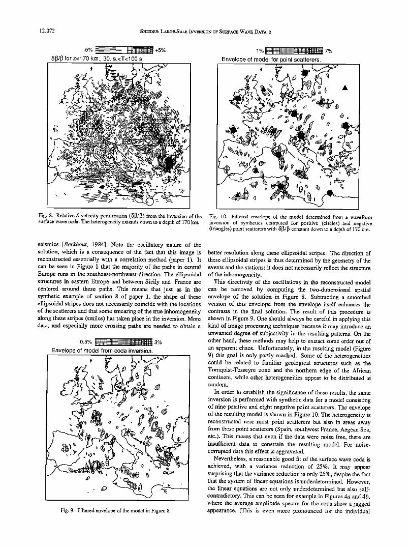
Fig. 8. Relative S velocity perturbation ([•/•) from the inversion of the surface wave coda. The heterogeneity extends down to a depth of 170 km.

Envelope of model for point scatterers.

Fig. 10. Filtered envelope of the model determined from a waveform inversion of synthetics computed for positive (circles) and negative (triangles) point scatterers with [•/• constant down to a depth of 170 km.

seismics [Berkhout, 1984]. Note the oscillatory nature of the solution, which is a consequence of the fact that this image is better resolution along these ellipsoidal stripes. The direction of reconstructed essentially with a correlation method (paper 1). It these ellipsoidal stripes is thus determined by the geometry of the can be seen in Figure 1 that the majority of the paths in central Europe runs in the southeast-northwest direction. The ellipsoidal structures in eastern Europe and between Sicily and France are centered around these paths. This means that just as in the synthetic example of section 8 of paper 1, the shape of these ellipsoidal stripes does not necessarily coincide with the locations of the scatterers and that some smearing of the true inhomogeneity along these stripes (smiles) has taken place in the inversion. More data, and especially more crossing paths are needed to obtain a

0.5% .......... ',1111',1111111• 3% Envelope of model from coda inversion.

Fig. 9. Filtered envelope of the model in Figure 8.

events and the stations; it does not necessarily reflect the structure of the inhomogeneity.

This directivity of the oscillations in the reconstructed model can be removed by computing the two-dimensional spatial envelope of the solution in Figure 8. Subtracting a smoothed version of this envelope from the envelope itself enhances the contrasts in the final solution. The result of this procedure is shown in Figure 9. One should always be careful in applying this kind of image processing techniques because it may introduce an unwanted degree of subjectivity in the resulting patterns. On the other hand, these methods may help to extract some order out of an apparent chaos. Unfortunately, in the resulting model (Figure 9) this goal is only partly reached. Some of the heterogeneities could be related to familiar geological structures such as the Tomquist-Tesseyre zone and the northern edge of the African continent, while other heterogeneities appear to be distributed at random.

In order to establish the significance of these results, the same inversion is performed with synthetic data for a model consisting of nine positive and eight negative point scatterers. The envelope of the resulting model is shown in Figure 10. The heterogeneity is reconstructed near most point scatterers but also in areas away from these point scatterers (Spain, southwest France, Aegean Sea, etc.). This means that even if the data were noise free, there are insufficient data to constrain the resulting model. For noise- corrupted data this effect is aggravated.

Nevertheless, a reasonable good fit of the surface wave coda is achieved, with a variance reduction of 25%. It may appear surprising that the variance reduction is only 25%, despite the fact that the system of linear equations is underdetermined. However, the linear equations are not only underdetermined but also self- contradictory. This can be seen for example in Figures 4a and 4b, where the average amplitude spectra for the coda show a jagged appearance. (This is even more pronounced for the individual

SNIEDER: LAR6E-SALE INVERSION OF SURFACE WAVE DATA, 2 12,073

Fit of (coda)data and synthetics, for T>50 s. I I I ' I

-- data

........ synthetics 5300NE15

5300NE04

3218NE12

o- 3218NE02 - _. . . .__ __• I I I I

600 800 1000 1200

time (s)

Fig. 1 la. Examples of the waveform fit of the surface wave coda, low passed at a comer period of 50 s.

spectra.) The scattering theory leads, in general, to much smoother spectra, so that it is impossible to fit all spectral components perfectly, thus producing an imperfect variance reduction.

Some waveform fits of the surface wave coda are shown in

Figures 11a and 1 lb both low passed and high passed at a comer period of 50 s. For periods larger than 50 s (Figure 11a) the waveform fit is poor. This is consistent with the results of section 2, where it was argued that the coda level does not stand out very well above the noise level. However, for the higher frequencies (periods from 30 to 50 s, see Figure 1 lb) a reasonable waveform fit is obtained. Most of the beats in the surface wave coda are

reproduced in the synthetics. It should be remembered that the seismograms in these figures only show the surface wave coda. In order to see these data in their proper perspective, a fit of the coda (band passed for periods between 30 s and 50 s) is shown in Figure 12 together with the direct wave. Unfortunately, the fact that good waveform fits are achieved does not establish the reliability of the resulting models because the linear system of equations is underdetermined.

Fit of (coda)data and synthetics, for 30 s.<T<50 s. ' I ' I ' I ' I

data

....... synthetics

. 5300NE04

3218NE12 -- - . - - ,, '... ,• o 3218NE02

I I I I

600 800 1000 1200

• time (s)

Fig. 1 lb. Examples of the waveform fit of the surface wave coda, high passed at a comer period ,of 50 s.

/

Event 3218 (Greece), station NE02. I ' I ' I

data

........ synthetics

I I I [ I t I

400 600 800 1000 1200

time (s)

Fig. 12. Full waveform fit of the surface wave coda, high passed at a comer period of 50 s.

Inversions for heterogeneities which extend to a depth different from 170 km produce almost the same model; only the strengths of these heterogeneities differs from the model shown in Figure 8. An inversion for data band passed between 30 and 40 s gives virtually the same result as Figure 8, which confirms that for longer periods the surface wave coda contains a large noise component and not much scattered surface waves.

These results do not imply that mapping lateral heterogeneity using the surface wave coda is impossible. In fact, it has been shown in a controlled field experiment that successful imaging of the surface wave coda is possible [Snieder, 1987a]. However, the surface wave coda data at our disposal are currently too sparse to produce an accurate reconstruction of the lateral heterogeneity. This is exacerbated by the fact that the noise level in the surface wave coda is relatively high, which can only be compensated with a redundant data set. Large networks of digital seismic stations, as formulated in the ORFEUS [Nolet et al., 1985] and PASSCAL proposals, are necessary to achieve this goal. Alternatively, the Born inversion of the surface wave coda might be used in regional studies where one wishes to study tectonic features such as continental margins or the boundaries of major geological formations. A system of portable digital seismographs would be very useful for this kind of investigations.

The directivity of the solution in Figure 8 is related to the source-receiver geometry. This means that apart from a denser network of stations, we should aim to employ these station in such a way that the wave paths of the recorded waves cover the domain of interest in a more or less homogeneous fashion. Furthermore, three-component data might help to constrain the location of the inhomogeneity because the horizontal components implicitly contain information on the backazimuth from the receiver to the

scatterer. Numerical experiments, similar to the experiment that produced Figure 10, could be used to determine which station configuration should be used to image a particular structure. In this way, the design of networks can be related to a particular geophysical or geological problem.

6. BORN INVERSION OF TI-tE DIRECT SURFACE WWAVE

Linear scattering theory can also be used to describe the distortion of the direct wave [Snieder, 1987b]. This distortion can

12,074 SNIEDER: LARGE-SALE INVERSION OF SURFACE WAVE DATA, 2

•c/c for 30 s.<T<40 s. after Born inversion.

Fig. 13a. Relative phase velocity perturbation (•c/c ) for periods between 30 and 40 s as determined from nonlinear waveform inversion plus a subsequent Born inversion. The dominant wavelength of the employed waves is shown for comparison.

either be due to ray geometrical effects or to multipathing effects that are not accounted for by ray theory. In the Born inversion presented in this section, the isotropic approximation is used (paper 1). This means that the relative phase velocity perturbations are retrieved from the linear waveform inversion of the direct wave. This quantity is assumed to be constant within the frequency bands employed (30-40 s, 40-60 s and 60-100 s).

(Note that in contrast to the case for the surface wave coda, the direct wave stands out well above the noise level for all employed frequencies; see Figures 4a and 4b.) A separate Born inversion is performed for each of these frequency bands, so that the phase velocity perturbation is determined independently for each frequency band. In order to justify the isotropic approximation (paper 1), a time window is used to extract the direct wave from the complete seismograms.

The Born inversions presented here are performed for a model of 100x100 cells with a cell size of 35x35 km 2. In the Born

inversion of the surface wave coda in section 5, no a priori smoothness constraint was imposed because scattered surface waves are most efficiently generated by sharp lateral heterogeneities. This led to an underdetermined system of linear equations. For the Born inversion of the direct wave the available data set also produces an underdetermined system of linear equations. One alternative would be to increase the cell size, but according to the example of Figure 7 in paper 1, rather small cells are needed to produce the required focusing/defocusing. Instead of this, the smoothing operator of equation (26) in paper 1 is used in this inversion to constrain the solution. In these inversions the

values ct•-0.66 and N=4 are used, which implies an effective correlation length of 140 km. The Born inversions are performed in three iterations (see also paper 1); it has been checked that more iterations do not change the resulting models very much.

The phase velocity perturbation for the three frequency bands are shown in Figure 13. The phase velocities are the result of both the nonlinear inversion for the smooth reference medium and the

subsequent Born inversion. See Figure 7b as an example of the contribution of the nonlinear inversion for the smooth reference

medium to the phase velocity model of Figure 13c. Note that the resulting phase velocity patterns vary

considerably on a scale of one horizontal wavelength. This means that ray theory cannot be used to model the effects of these heterogeneifies, while surface wave scattering theory takes effects such as multipathing into account. Surprisingly, Figure 13c for the phase velocity determined from Born inversion is not too different from Figure 7a for the unconstrained nonlinear inversion using

-5% +5O/o -5% h-=- +5O/o (5c/c for 40 s.<T<60 s. after Born inversion. (5c/c for 60 s.<T<100 s. after Born inversion.

for T=75 s.

Fig. 13b. As Figure 13a, but for periods between 40 and 60 s. Fig. 13c. As Figure 13a, but for periods between 60 and 100 s.

$NIEDER: LARGE-SALE •¾ERSION OF SURFACE WAVE DATA, 2 12,075

Event 3218 (Greece), station NE12, 30 s.<T<40 s. I ' I ' I I '

data ,,,

',,;

I , I I I ,

500 600 700 800

time (s)

Fig. 14. Waveform fit for periods between 30 and 40 s for the laterally homogeneous starting model (top), after the nonlinear inversion for a smooth reference model (middle), and after Born inversion (bottom), for a Greek event recorded in NE12 (Spain).

ray theory. The smaller-scale features of Figure 13c are absent in Figure 7a because the spline interpolation does not allow these small-scale features (nor does ray theory). Nevertheless, the overall pattern in these Figures is the same. Apparently, ray theory is rather robust to violations of the requirement that the heterogeneity is smooth. This may explain the success of dispersion measurements in situations where ray theory is not justified. Most of the information on the S velocity structure under Europe in the crust and upper mantle is determined from surface wave dispersion measurements. For example, Panza et al. [1982] delineated a heterogeneity between Corsica and northern Italy with a scale of approximately 250 km, from anomalously low Rayleigh wave phase velocities between 40 and 60 s. Their results are therefore inconsistent with the (ray) theory that they employed. Nevertheless, this low phase velocity anomaly is also visible in Figure 13b, which is constructed using surface wave scattering theory.

Event 5300 (Algeria), stakon NE15, 40 s.<T<60 s. ' I I I I

data

...... synthetics

:"/• /"• ::/• lat. hom.

'" "•, northnear fit

400 500 600 700

hme (s)

Fig. 16. As Figure 14 for an Algerian event recorded in NE15 (Netherlands) for periods between 40 and 60 s.

Waveform fits after the nonlinear inversion for the smooth

reference model and after the subsequent Born inversion (the "final fit") are shown in Figures 14-19. In Figure 14, results for station NE12 near Madrid are shown. The amplitude of the direct surface wave is changed considerably in the inversion. Note that the waveform fit has slightly deteriorated in the nonlinear inversion. The reason for this is that the 42 seismograms are inverted simultaneously, so that it is possible that the fit of one seismogram is improved at the expense of another seismogram. In Figure 15 an example is shown for a seismogram recorded at NE01 (Gothenborg). For this seismogram the amplitude is already quite good for the laterally homogeneous starting model, but the phase is adjusted in the Born inversion. In the preceding examples the Born inversion realized the fit between data and synthetics. This is not the case for all seismograms. In Figure 16 a seismogram for an event in Algeria recorded at NE15 (Netherlands) is shown. For this seismogram the nonlinear inversion performed most of the waveform fit.

By superposing the seismograms for the three frequency bands, seismograms for the full bandwidth (30-100 s) can be

Event 4042 (Greece), station NE01,30 s.<T<40 s. I I I ' I ' I '

- data . :', m

' '" '" "i'", "% ear fit

., "", ' ' ! i ,,: final fit

I , I , I I •

500 600 700 800

time (s)

Fig. 15. As Figure 14, for a Greek event recorded in NE01 (Oothenborg) for periods between 30 and 40 s.

Event 3218 (Greece), station NE12, 30 s.<T<100 s. I ' I ' I ' I '

- data

........ synthetics /r• :,,• .

500 600 700 800 time (s)

Fig. 17. As Figure 14 for the full bandwidth (30-100 s).

12,076 SNIEDER: LARGE-SALE •WERSION OF SURFACE WAVE DATA, 2

Event 5300 (Algeria), station NE15, 30 s.<T<100 s. ' i ,

data

nonlinear fit

ß .

, I I I , I

400 500 600 700

time (s)

Fig. 18. As Figure 14 for the full bandwidth (30-100 s).

constructed. Figure 17 displays the seismogram of Figure 14, but now for the full employed bandwidth. The final fit between the data and the synthetic is extremely good. Note that the tail of the direct wave (around 725 s) is fitted quite well after the Born inversion. For the recording of the Algerian event in NE15, the full bandwidth data are shown in Figure 18. The trough in the waveform around 420 s has been adjusted well in the nonlinear inversion, whereas the fit of the start of the signal (around 400 s) is improved considerably in the subsequent Born inversion. Unfortunately, the improvement in the waveform fits is not for all seismograms as dramatic as in the preceding examples. Figure 19 features the waveform fit for a Greek event recorded at NE02 (Denmark). The phase of the signal is slightly improved in the nonlinear inversion, but the final waveform fit is not impressive.

The quality of the waveform fits is expressed by the variance reductions shown in Table 1. Both in the nonlinear inversion and in the subsequent Born inversion the variance reduction is of the order of 25%, although this differs considerably between the different frequency bands. In the nonlinear inversion for the

TABLE 1, Variance Reductions for the Waveform Inversions

Period, s Nonlinear Bom Nonlinear +Bom 30-40 15% 20% 31% 40-60 37% 27% 54%

60-100 21% 25% 41%

smooth reference medium the solution is rather heavily constrained (compare Figures 7a and 7b) so that larger variance reductions could be achieved with the nonlinear inversion. The

smallest variance reduction occurs in the period range from 30 to 40 s. This is not surprising because these surface waves have the shallowest penetration depths and are therefore most strongly subjected to lateral heterogeneity and therefore most difficult to fit. Surprisingly, the variance reduction for periods between 40to 60 s is larger than for 60-100 s. The reason for this might be that surface waves between 60-100 s. are influenced by the low- velocity zone, which is reported to exhibit strong lateral variations [York and Helmberger, 1973; Paulssen, 1987]. The total variance reduction is larger than the variance reduction obtained by Yomogida and Aki [1987] for surface waves which propagated through the Pacific. (They obtained a variance reduction of approximately 30%.) However, it is difficult to compare these results because on the one hand the paths of propagation of the surface waves that they used are much longer than in this study but on the other hand Europe and the Mediterranean is much more heterogeneous than the Pacific.

7. A RESOLUTION ANALYSIS OF TIlE INVERSION FOR THE DmECT WAVE

Just as with the inversion for the surface wave coda, the quality of the waveform fit is no measure of the resolution of the

inversion. In order to address this issue, synthetics have been

-s% h-- +s% 6c/c model for resolution experiment.

Event 3218 (Greece), station NE02, 30 s.<T<100 s. ' I , i , i ,

-- data

........ syni•eti•i .../f• ),,/) ,,"'-..'"' _. ß .

final fit

5OO 6OO 7OO

time (s)

Fig. 19. As Figure 14 for a Greek event recorded in NE02 (Denmark) for the full bandwidth (30-100 s).

Fig. 20. Synthetic model of the relative phase velocity perturbation (•5c/c ) for the resolution experiment of section 7. The source-receiver minor arcs are superposed.

SNIEDER: LARGE-SALE INWERSION OF SURFACE WAVE DATA, 2 12,077

,5c/c model after nonlinear inversion, 60 s.<T<100 s.

wave paths runs in a bundle from Greece to northwestern Europe and encounters a suite of positive and negative anomalies. This leads to a smearing of the solution under Germany and Denmark in the northwest-southeast direction and a subsequent underestimate of the true inhomogeneity. A similar smearing in the northwest-southeast direction is visible in the northern

Adriatic; this area also suffers from a lack of crossing ray paths. One of the most conspicuous features in Figure 13 is the high phase velocities under Greece. This is no artifact of the inversion because this feature is not present in the results from the resolution analysis (Figure 22).

In conclusion, the reconstructed phase velocity models are meaningless outside the dotted line in Figures 24 and 25. In the area enclosed by this line, lateral smearing in the northwest- southeast direction occurs under Denmark, Germany, and the northern Adriatic, while there is an east-west smearing in the southern Mediterranean.

8. A MODEL FOR TIDES VELOCITY UNDER EUROPE

AND Tim MEDiTERRANEAN

The phase velocity perturbations presented in section 6 can be converted to a depth model using the phase velocity information

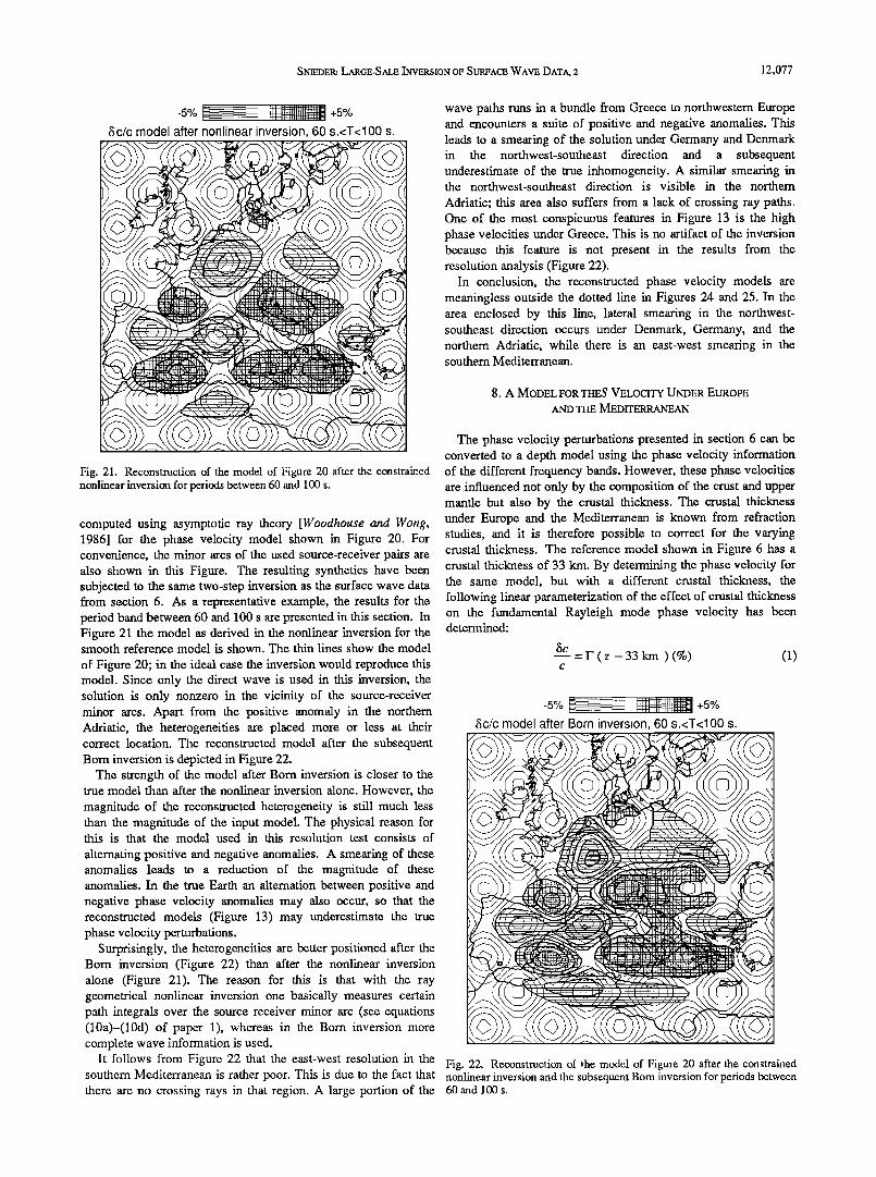
Fig. 21. Reconstruction of the model of Figure 20 after the constrai•.ed nonlinear inversion for periods between 60 and 100 s.

computed using asymptotic ray theory [Woodhouse and Wong, 1986] for the phase velocity model shown in Figure 20. For convenience, the minor arcs of the used source-receiver pairs are also shown in this Figure. The resulting synthetics have been subjected to the same two-step inversion as the surface wave data from section 6. As a representative example, the results for the period band between 60 and 100 s are presented in this section. In Figure 21 the model as derived in the nonlinear inversion for the smooth reference model is shown. The thin lines show the model

of Figure 20; in the ideal case the inversion would reproduce this model. Since only the direct wave is used in this inversion, the solution is only nonzero in the vicinity of the source-receiver minor arcs. Apart from the positive anomaly in the northern Adriatic, the heterogeneities are placed more or less at their correct location. The reconstructed model after the subsequent Born inversion is depicted in Figure 22.

The strength of the model after Born inversion is closer to the true model than after the nonlinear inversion alone. However, the

magnitude of the reconstructed heterogeneity is still much less than the magnitude of the input model. The physical reason for this is that the model used in this resolution test consists of

alternating positive and negative anomalies. A smearing of these anomalies leads to a reduction of the magnitude of these anomalies. In the true Earth an alternation between positive and negative phase velocity anomalies may also occur, so that the reconstructed models (Figure 13) may underestimate the true phase velocity perturbations.

Surprisingly, the heterogeneities are better positioned after the Born inversion (Figure 22) than after the nonlinear inversion alone (Figure 21). The reason for this is that with the ray geometrical nonlinear inversion one basically measures certain path integrals over the source receiver minor arc (see equations (10a)-(10d) of paper 1), whereas in the Born inversion more complete wave information is used.

It follows from Figure 22 that the east-west resolution in the

of the different frequency bands. However, these phase velocities are influenced not only by the composition of the crust and upper mantle but also by the crustal thickness. The crustal thickness under Europe and the Mediterranean is known from refraction studies, and it is therefore possible to correct for the varying crustal thickness. The reference model shown in Figure 6 has a crustal thickness of 33 km. By determining the phase velocity for the same model, but with a different crustal thickness, the following linear parameterization of the effect of crustal thickness on the fundamental Rayleigh mode phase velocity has been determined:

5c • = F ( z - 33 km ) (%) (1)

c

6c/c model after Born inversion, 60 s.<T<100 s.

Fig. 22. Reconstruction of ,he model of Figure 20 after the constrained southern Mediterranean is rather poor. This is due to the fact that nonlinear inversion and the subsequent Born inversion for periods between there are no crossing rays in that region. A large portion of the 60 and 100 s.

12,078 SNIEDER: LARGE-SALE •WERSION OF SURFACE WAVE DATA, 2

Smoothed crustal thickness in domain.

Fig. 23. Smoothed crustal thickness used in the correction for the varying Moho depth.

in this expression, z is the crustal thickness in kilometers. The parameter F is for the different frequency bands given by

F=-0.180(%/km) for 30s<T<40s

F=-0.113 (%/km) for 40s<T<60s (2)

F=-0.076(%/km) for 60s<T<100s

The crustal thickness used in this study is adopted from

same smoothing is applied to the crustal thickness, as for the reconstructions shown in Figure 13. The variations in the crustal thickness are as large as 25 km in the area of interest. For the shortest-period band this leads to a phase velocity perturbation of 4.5%, which is of the same order of magnitude as the perturbations as determined from the Born inversion (Figure 13a).

After correcting for the crustal thickness, a standard linear inversion [Nolet, 1981] leads to the S velocity perturbations for depths between 0 and 100 km, and between 100 and 200 km. A simple resolution analysis shows that incorporating a third layer is unjustified. The resulting S velocity perturbations are shown in Figures 24 and 25. A bias in the S velocity of the reference model would show up as a dominance of either positive or negative velocity perturbations. Likewise, a bias in the attenuation would show up in structures that would for the majority of the paths produce a marked focusing or defocusing. As can be seen from Figures 24 and 25, and from the wave paths in Figure 1, neither effect seems to be present.

The S velocity models in these Figures can be compared with maps of the S velocity as compiled subjectively from a wide range of surface wave and body wave data [Panza et al., 1980; Calcagnile and Scarpa, 1985]. In general, there is a correspondence of the large-scale features. The velocity is high in the Scandinavian shield, which can be seen in the northern area of inversion of Figures 24 and 25. Under the western Mediterranean the velocity is low [Marillier and Mueller, 1985], whereas the Adriatic is characterized by a S velocity higher than in the adjacent regions. This high velocity under the Adriatic is more pronounced in the lowest layer (Figure 25) than in the top layer (Figure 24). Note that the Alps do not show up in Figures 24 and 25, whereas Panza et al. [1980] and Calcagnile and Scarpa [1985] report large anomalies both in the western Alps and the eastern Alps. A reason for this discrepancy might be that the

Meissner [1986] and Stoko et al. [1987], and is shown in Figure depth-averaged structure of the Alps deviates not very much from 23. In the area outside the dotted line in Figures 24 and 25 the the rest of Europe, so that the surface waves are not perturbed default value is assumed (33 km). For consistency reasons, the strongly.

-s% +s% for 0 km.<z<100 km.

-5% +5O/o (513/13 for 100 km.<z<200 km.

Fig. 24. Relative S velocity perturbation ([•/•) between the surface and a Fig. 25. Relative S velocity perturbation ([•/•) for depths between 100 depth of 100 km. and 200 km.

$NIEDER: LARGE-SALE INVERSION OF $U•ACE WAVE DATA, 2 12,079

Early tomographic studies using P wave delay times [Romanowicz, 1980; Hovland et al., 1981; Hovland and Husebey, 1982; Babuska et al., 1984] produced rather different results for the P velocity under Europe. The only consistent features of these studies are the low velocity in the Pannonian basin and the high velocity under the Bohemian massif for the upper layer (0-100 km). Both features can also be seen in Figure 24. (In Figure 23 the Pannonian basin shows up as a region with a thin crust, whereas the Bohemian massif can be identified by its thick crust.) A more recent tomographic inversion with a much larger data set produced more detailed results [Spakmart, 1986a,b; Spakmart et al., 1988]. In his studies the subduction of Africa under Europe has been imaged spectacularly. The subduction of Africa of the African slab under Europe can also be seen in Figure 25 as a positive velocity anomaly in the deepest layer (100-200 km) under the Adriatic and northern Italy. Panza et al. [1982] observed relatively low velocities in the lid between Corsica and Italy; the same anomaly is visible in Figure 24.

In Figures 24 and 25 the Rhine Graben shows up as a zone of relatively low velocities extending toward the southeast from the Netherlands. Most wave paths in this region are in the southeast- northwest direction. This may explain why in the top layer (Figure 24) only the northern part of the Rhine Graben can be seen, whereas the southern part of the Rhine Graben (which trends in the north-south direction) is not delineated. The variations in the S velocity for the deepest layer (Figure 25) reflect the lateral variations of the low-velocity zone. It is noted by York and Helmberger [1973] and Paulssen [1987] that strong velocity variations of the low-velocity zone exist, which is confirmed by Figure 25. Under the Massif Central the positive anomaly in the top layer (Figure 24) and the negative anomaly in the bottom layer (Figure 25) indicate a pronounced low-velocity zone, which is consistent with the results of Souriau [1981].

The feature which shows the power of the inversion method of this paper most spectacularly is the high-velocity anomaly in eastern Europe in the deepest layer (Figure 25). (It is possible that this area of high velocities extends farther eastward, but this area is not sampled by the data.) From the waveform point of view, this anomaly is needed to produce the focusing needed to fit the amplitudes of seismograms recorded in the northern station of the NARS array. For this reason, this anomaly is located away from (but close to) the source receiver minor arcs. This zone of a high S velocity closely marks the Tomquist-Tesseyre zone, the boundary between central Europe and the east European platform. Note that this transition zone is not visible in the upper layer of the S- velocity model (Figure 24). This is consistent with the findings of Hurtig et al. [1979], who showed by fitting travel time curves that below 100 km the eastern European platform has higher P velocities than central Europe. According to Figure 25 this transition at depth between Central Europe and the eastern European platform is very sharp.

The models presented produce a wealth of interesting features. However, at this point one should be extremely careful with a physical interpretation of these models. As shown by the resolution analysis of section 7, parts of these models are subjected to strong lateral smearing, which could produce unwanted artifacts. Furthermore, the number of seismograms that contributes to the reconstruction of a particular inhomogeneity is relatively small. This means that errors in individual seismograms can distort the reconstructed images. Larger data sets with a more even path distribution are needed to produce models which are less likely to contain artifacts and which are more robust to errors in individual seismograms.

9. CONCLUSION

Linear inversion of a large set of surface wave data is feasible with present-day computers. The Born inversion for the surface wave coda (using 42 seismograms) ran in roughly one night on a super minicomputer. The inversion of the direct surface wave for the three frequency bands takes approximately the same time. The nonlinear inversion for the smooth reference model is

comparatively fast and takes about 3 hours for the three frequency bands. With the present growth in computer power, larger data sets can soon be inverted with the same method, possibly on a global scale.

Reasonable waveform fits of the surface wave coda can be

obtained, leading to a variance reduction of approximately 25% for the surface wave coda. However, with the data set used in this

study many artifacts are introduced in the inversion (the analogue of the smiles in exploration seismics). The fact that the surface wave coda contains a relatively large noise component is an extra complication. A larger (redundant) data set is needed to perform an accurate imaging of the inhomogeneity in the Earth using the surface wave coda. It would be interesting to set up controlled experiments to probe tectonic structures like continental margins or the Tornquist-Tesseyre zone with scattered surface waves.

Application of Born inversion to the direct surface waves leads to detailed S velocity models on a scale conaparable to the wavelength of the surface waves used. With the data set employed, a lateral resolution of approximately 300 km can be achieved in some regions (Italy, France, Alps, western Mediterranean), while in other areas, smearing along the wave paths occurs (southern Mediterranean, northeastern Europe, the Adriatic). More data are needed to achieve a more evenly distributed resolution. Only a limited depth resolution can be obtained.

The fact that a model of the heterogeneity is constructed with a horizontal length scale comparable to the wavelength of the used surface waves implies that scattering and multipathing effects are operative. This means that for this situation, dispersion measurements are not justified. Nevertheless, the resulting model for the S velocity bears close resemblance to the S velocity models constructed by Panza et al. [1980] and Calcagnile and Sca•;pa [1985], which are largely based on surface wave dispersion measurements. Apparently, the phase as deduced from ray theory is relatively robust for structures that are not smooth on scale of a wavelength.

Linear waveform inversion is a powerful and rigorous method to fit surface wave data. Presently, the main limitation is imposed by the availability of high-quality digital surface wave data. A network of seismometers, as described in the ORFEUS [Nolet et al., 1985] or PASSCAL proposals, will increase the resolution and reliability of the resulting models. A data distribution center like ODC (ORFEUS Data Center) provides access to digital seismological data at low costs. Born inversion for surface waves, applied to these data, may help to construct accurate S velocity models of the Earth.

Acknowledgments. I thank Guust Nolet for his stimulating interest and advice for this research. His nonlinear waveform fitting program formed the backbone of the nonlinear waveform inversion presented in this study. Wire Spakman provided me kindly with his tomography program, which formed the basis for the software for the Bom inversion. The help of Gordon Shudofsky, Bemard Dost, and Hanneke Paulssen was indispensable for handling the NARS data. The constructive comments of Brian Mitchell and an anonymous reviewer are greatly appreciated. The NARS project has been funded by AWON, the Earth Science branch of the Netherlands Organization for the Advancement of Pure Research (ZWO).

12,080 SNIEDER: LARGE-SALE INVERSION OF SURFACE WAVE DATA, 2

REFERENCES

Babuska, V., J. Plomerova, and J. Sileny, Large-scale oriented structures in the subcrustal lithosphere of Central Europe, Ann. Geophys., 2, 649-662, 1984.

Berkhout, A.J., Seismic Migration, Imaging of Acoustic Energy by Wave FieM Extrapolation, B, Practical Aspects, Elsevier, Amsterdam, 1984.

Calcagnile, G., and R. Scarpa, Deep structure of the European- Mediterranean area from seismological data, Tectonophysics, ]]8, 93-111, 1985.

Chapman, C.H., The Radon transform and seismic tomography, in Seismic Tomography, With Applications in Global Seisinology and Exploration Geophysics, edited by G. Nolet, pp. 99-108, D. Reidel, Hingham, Mass., 1987.

Dost, B., A. van Wetrum, and G. Nolet, The NARS array, Geol. Mijnbouw, 63, 381-386, 1984.

Dziewonski, A.M., Mapping the lower mantle: Determination of lateral heterogeneity in P velocity to degree and order 6, J. Geophys. Res., 89, 5929-5952, 1984.

Dziewonski, A.M., and D.L. Anderson, Preliminary reference Earth model, Phys. Earth Planet. Inter., 25, 297-356, 1981.

ttovland, J., and E.S. Husebye, Upper mantle heterogeneities beneath eastem Europe, Tectonophysics, 90, 137-151, 1982.

Hovland, J., D. Gubbins, and E.S. Husebye, Upper mantle heterogeneities beneath central Europe, Geophys. J. R. Astron. Soc., 66, 261-284, 1981.

Hurtig, E., S. Grassl, and R.P. Oesberg, Velocity variations in the upper mantle beneath central Europe and the east European platform, Tectonophysics, 56, 133-144, 1979.

Incorporated Research Institute for Seismology, PASSCAL, Program for Array Studies of the Continental Lithosphere, 1984.

Marillier, F., and S. Mueller, The westem Mediterranean region as an upper mantle transition zone between two lithospheric plates, Tectonophysics, 118, 113-130, 1985.

Meissner, R., The Continental Crust, A Geophysical Approach, Academic, San Diego, Calif., 1986.

Nataf, H.C., I. Nakanishi, and D.L. Anderson, Measurements of mantle wave velocities and inversion for lateral heterogeneity and anisotropy, 3, Inversion, J. Geophys. Res., 9], 7261-7308, 1986.

Nolet, G., The upper mantle under Western-Europe inferred from the dispersion of Rayleigh wave modes, J. Geophys., 43,265-285, 1977.

Nolet, G., Linearized inversion of (teleseismic) data, in The Solution ofthe Inverse Problem in Geophysical Interpretation, edited by R. Cassinis, pp. 9-38, Plenum, New York, 1981.

Nolet, G., B. Romanowicz, R. Kind, and E. Wielandt, ORFEUS, Observatories and Research Facilities for European Seismology, 1985.

Nolet, G., B. Dost, and II. Paulssen, Intermediate wavelenglh seismology and the NARS experiment, Ann. Geophys., B4, 305-314, 1986.

Panza, G.F., S. Mueller, and G. Calcagnile, The gross features of the lithosphere-asthenosphere system from seismic surface waves and body waves, Pure Appl. Geophyx., 118, 1209-1213, 1980.

Panza, G.F., S. Mueller, G. Calcagnile, and L. Knopoff, Dclinealion of the noah central Italian upper mantle anomaly, Nature, 296, 238-239, 1982.

Paulssen, II., Lateral hetcrogeneity of Europc's upper mantle as inferred froin modelling of broad-band body waves, Geophys. J. R. Astron. Soc., 91,171-199, 1987.

Romanowicz, B., A study of large-scale lateral variations of P velocity in the upper mantle beneath western Europe, Geophys. J. R. Astron. Soc., 63,217-232, 1980.

Romanowicz, B., and R. Snieder, A new formalism for the effect of lateral heterogeneity on normal modes and surface waves, 1I: General anisotropic perturbations, Geophys. J. R. Astron. Soc., 93, 91-100, 1988.

Snieder, R., 3D Linearized scattering of surface waves and a formalism for surface wave holography, Geophys. J. R. Astron. Soc., 84, 581-605, 1986a.

Snieder, R., The influence of topography on the propagation and scattering of surface waves, Phys. Earth Planet. Inter., 44, 226-241, 1986b.

Snieder, R., Surface wave holography, in Seismic Tomography, With Applications in Global Seisinology and Exploration Geophysics, edited by G. Nolet, pp. 323-337, D. Reidel, Hingham, Mass., 1987a.

Snieder, R., On the connection between ray theory and scattering theory for surface waves, in Mathematical Geophysics, A Survey of Recent Developments in Seisinology and Geodynamics, edited by N.J. Vlaar, G., Nolet, M.J.R., Wonel, S.A.P.L. and Cloetingh, pp. 77-83, D. Reidel, Hingham, Mass., 1987b.

Snieder, R., Large-scale waveform inversions of surface waves for lateral heterogeneity, 1, Theory and numerical examples, J. Geophys. Res., this issue, 1988.

Snieder, R., and G. Nolet, Linearized scattering of surface waves on a spherical Earth, J. Geophys., 6], 55-63, 1987.

Snieder, R., and B. Romanowicz, A new formalism for the effect of lateral heterogeneity on normal modes and surface waves, I, Isotropic perturbations, perturbations of interfaces and gravitational perturbations, Geophys. J. R. Astron. Soc., 92, 207-222, 1988.

Souriau, A., Le manteau superieur sous la France, Bull. Soc. Geol. Fr., 23, 65-81, 1981.

Spakman, W., Subduction beneath Europe in connection with the Mesozoic Tethys, Geol. Mijnbouw, 65, 145-154, 1986a.

Spakman, W., The upper mantle structure in the central European- Mediterranean region, in Proceedings of the Third Workshop on the European Geotraverse Project (EGT), pp. 215-221, 1986b.

Spakman, W., M.J.R. Wortel and N.J. Vlaar, The Hellenic subduction zone: A tomographic image and its geodynamic implications, Geophys. Res. Lett., 15, 60-63, 1988.

Stoko, D., E. Prelogovic, and B. Alinovic, Geological structure of the Earth's crust above the Moho discontinuity in Yugoslavia, Geophys. J. R. Astron. Soc., 89, 379-382, 1987.

Tanimoto, T., The three-dimensional shear wave velocity structure in the mantle by overtone waveform inversion, I, Radial seismogram inversion, Geophys. J. R. Astron. Soc., 89,713-740, 1987.

Van der Sluis, A., and H.A. Van der Vorst, Numerical solution of large, sparse linear algebraic systems arising from tomographic problems, in Seismic Tomography, With Applications in Global Seisinology and Exploration Geophysics, edited by G. Nolet, pp. 49-83, D. Reidel, Itingham, Mass., 1987.

Woodhouse, J.H., and A.M. Dziewonski, Mapping the upper mantle: Three-dimensional modeling of the Earth structure by inversion of seismic waveform, J. Geophys. Res., 89, 5953-5986, 1984.

Woodhouse, J.H., and Y.K. Wong, Amplitude, phase and path anomalies of mantle waves, Geophys. J. R. Astron. Soc., 87, 753-774, 1986.

Yomogida, K., and,K. Aki, Amplitude and phase data inversion for phase velocity anomalies in the Pacific Ocean basin, Geophys. J. R. Astron. Soc., 88, 161-204, 1987.

York, J.E., and D.V. llelmberger, Low-velocity zone variations hi the southwestern United States, J. Geophys. Res., 78, 1883-1886, 1973.

R. Snicder, Department of Theoretical Geophysics, University of Utrecht, P.O. Box 80.021, 3508 TA Utrechi, The Netherlands.

(Received October 22, 1987; revised April 21, 1988;

accepted April 25, 1988.)