Large&scale geomorphology: Classical concepts reconciled ...geomorphology.sese.asu.edu/Papers/Kooi_and_Beaumont_1996_JGR.pdf · JOURNAL OF GEOPHYSICAL RESEARCH, VOL. tot, NO. B2,

JOURNAL OF GEOPHYSICAL RESEARCH, VOL. tot, NO. B2, PAGES 3361-3386, FEBRUARY t0, 1996

Large-scale geomorphology: Classical concepts reconciled and integrated with contemporary ideas via a surface processes model

Henk Kooi and Christopher Beaumont Department of Oceanography, Dalhousie University, Halifax, Nova Scotia, Canada

Abstract. Linear systems analysis is used to investigate the response of a surface processes model (SPM) to tectonic forcing. The SPM calculates subcontinemal scale denudational landscape evolution on geological timescales (1 to hundreds of million years) as the result of simultaneous hillslope transport, modeled by diffusion, and fluvial transport, modeled by advection and reaction. The tectonically forced SPM accommodates the large-scale behavior envisaged in classical and contemporary conceptual geomorphic models and provides a framework for their integration and unification. The following three model scales are considered: micro-, meso-, and macroscale. The concep• of dynamic equilibrium and grade are quantified at the microscale for segmems of uniform gradient subject to tectonic uplift. At the larger meso- and macroscales (which represent individual interfluves and landscapes including a number of drainage basins, respectively) the system response to tectonic forcing is linear for uplift geometries that are symmetric with respect to baselevel and which impose a fully integrated drainage to baselevel. For these linear models the response time and the transfer function as a function of scale characterize the model behavior. Numerical experiments show that the styles of landscape evolution depend critically on the timescales of the tectonic processes in relation to the response time of the landscape. When tectonic timescales are much longer than the landscape response time, the resulting dynamic equilibrium landscapes correspond to those envisaged by Hack (1960). When tectonic timescales are of the same order as the landscape response time and when tectonic variations take the form of pulses (much shorter than the response time), evolving landscapes conform to the Penck type (1972) and to the Davis (1889, 1899) and King (1953, 1962) type frameworks, respectively. The behavior of the SPM highlights the importance of phase shifts or delays of the landform response and sediment yield in relation to the tectonic forcing. Finally, nonlinear behavior resulting from more general uplift geometries is discussed. A number of model experiments illustrate the importance of "fundamental form" which is an expression of the conformity of antecedent topography with the current tectonic regime. Lack of conformity leads to models that exhibit internal thresholds and a complex response.

Introduction

It becomes increasingly important to understand erosional denudation on geological timescales (105 -109 years) as our understanding of geological subsystems, such as sedimentary basins, compressional orogens, and rifts, increases. Many recent papers argue the importance of or explore the role of (1) flexural isostatic feedback between erosion and deposition [Flemings and Jordan, 1989; Sinclair et al., 1991; Johnson and Beaumont, 1995], (2) climate coupling and erosional control of the exhumation and deformation in compressional orogens [Koons, 1989; Beaumont et al., 1992; Hoffman and Grotzinger, 1993], (3) complex response and the associated temporal and spatial

Copyright 1996 by the American Geophysical Union.

Paper number 95JB01861. 0148-0227/96/95JB-01861 $05.00

variability of sediment transport in the production of stratigraphic sequences [Schumm, 1980, 1993; Wescott, 1993], and (4) the relative importance of tectonics and climate in mountain building [Molnar and England, 1990; England and Molnar, 1990].

Two related ideas that may lead to a tangible framework for the study of landscape evolution on geological timescales appear frequently in papers published during the last three decades. (1) Large-scale, long-term landscape evolution can be viewed as the behavior of a process response system. It follows that the behavior can be studied by methods of system analysis if the system can be quantified [e.g., Chorley, 1962; Howard, 1965, 1982; Huggett, 1988; Phillips and Renwick, 1992]. (2) Classical conceptual geomorphic models may be valid under specific tectonic, climatic, and substrate conditions and at specific scales [e.g., Higgins, 1980; Palrnquist, 1980]. These ideas imply that apart from some claims to universal applicability, there may be no conflict among the various classical

3361

3362 KOOI AND BEAUMONT: LARGE-SCALE GEOMORPHOLOGY

conceptual models and that these models might be reconciled with modem concepts within a single numerical framework.

Inspired by these ideas, we take a practical approach to large-scale long-term landscape evolution. We quantify the geomorphic system in a simplified, process-based form and investigate the behavior of this surface processes model (SPM) systematically to see to what extent and under what conditions it accommodates the various geomorphic concepts, an approach advocated by Tinkler [1985, p. 238]. The same approach can be taken for alternative process formulations, as in the smaller-scale examples [e.g., Willgoose et al., 199 la; Howard, 1994], and a comparison made of the behavioral characteristics. Also, since an SPM makes predictions for all its component parts, these predictions can be compared with the fragmentary geomorphic record in an integrated manner. Such an approach is commonly used when scientific problems are too complex for direct inductive solution and is not generally regarded a priori to be a sterile exercise [Ritter, 1988], even if a unique solution does not emerge.

The development of SPMs is not new. In recent years, Ahnert [1976, 1987a, b], Kirkby [1986], Chase [1992], Willgoose et al. [1991a, b], Beaumont et al. [1992]; Tucker and Slingerland [1994], and Howard [1994], for example, have developed and studied the behavior of SPMs that includes interactions among a small number of processes that are individually relatively simple and that operate on planform (two-dimensional) model topographies. Most of these studies investigate model behavior of either single catchments or hillslopes or small areas and relate model predictions to geomorphic concepts appropriate for these scales [e.g., Ahnert, 1987b; Willgoose et al., 1991a; Howard, 1994], regional observations [e.g., Rosenbloom and Anderson, 1994], and/or empirical relationships [Willgoose et al., 1992; Willgoose, 1994a]. Chase [1992] and Tucker and Slingerland [1994] employ their SPMs at scales larger than single catchments (subcontinental scale) but do not compare restfits with classical geomorphic models.

and the concept of grade. At the larger meso- and macroscales (defined at the scale of interfluves and landscapes including a number of catchments, respectively) we require the SPM for illustrative model experiments, and the analysis for these scales is made concurrently.

At each of the scales we investigate the steady stat•$ of the system when the external controls are held constant. The system response is then shown to be linear for certain tectonic uplift geometries, where the spatial distribution is simple and remains constant. For these linear models the response time and transfer function as a function of scale characterize the model behavior. Model experiments are used to show that basic forms of landform evolution envis-

aged by Davis [1889,1899], Penck [1972], Hack [1960], and King [1953,1962] occurs, depending on the timescales of the tectonic processes in relation to the response time of the landscape. Finally, we illustrate the importance of "fundamental form" [Brice, 1964] using a number of model experiments. Fundamental form is interpreted as an expression of the conformity (or sympathetic nature) of antecedent topography with the new tectonic geometry. Lack of conformity leads to geometrical nonlinearity in the model response. Models of this type exhibit a complex response.

The Surface Processes Model

Model Formulation

The SPM [Beaumont et al., 1992; Kooi and Beaumont, 1994] simulates erosional denudation at spatial scales of 1 to hundreds of kilometers and timescales of 1 to hundreds

of million years. It calculates long-term changes in topography h that result from simultaneous short- and long-range mass transport processes using a combination of diffusion, advection, and reaction. Short-range transport represents the cumulative effects of hillslope processes and is modeled as linear diffusion

dh / dt = KsV2h, (1)

Focus and Organization

In this paper we briefly review and use a SPM [Beaumont et al., 1992; Kooi and Beaumont, 1994] that is designed for subcontinental scales and compare its behavior with landscape evolution envisaged in conceptual models. The central theme is to point out that (1) many apparently incompatible conceptual interpretations of landscapes and their evolution are not necessarily incompatible (even though some were claimed to be universal) and (2) they can be viewed as different styles of behavior in a single simple system when different processes dominate. Among the range of potential controls, we focus on the roles of tectonics and antecedent topography, factors which were found to be primary in the integration of the classical conceptual geomorphic models in the SPM. This approach does not assume these concepts to be valid or prove them to be so. It only shows how they may be reconciled.

We consider the following three scales: micro-, meso-, and macroscale. At the microscale, uniform gradient segments of landforms are analyzed analytically for their characteristic behavior in relation to dynamic equilibrium

with diffusivity K s , which is interpreted to depend on both climate and substrate. Long-range transport represents fluvial transport in which the equilibrium fiver sediment carrying capacity, qeqb=-K qrdh/dl, is a linear func- ß of. f laon of the local discharge qr, and the local downstream slope dh/d/, and Kœ is a nondimensional transport coefficient. Discharge-is the result of precipitation VR distributed over the model topography and collected by rivers that follow routes of steepest descent. It is not assumed that the fluvial transport system is everywhere carrying at capacity. Instead, fluvial entrainment of the sediment flux qf is controlled by an erosion length scale l f, a measure of the detachability of the substrate.

c}h / c}t = -dq f / dl = -(1 / l f )(q•qb _ q f ).

A high value of lf_ corresponds to a low detachability, and the converse is also tr0. e. The reaction is driven by the local undercapacity (q•qV _ qœ ) of the fiver.

The present appro•ich differs from other formulations [e.g., Willgoose et al., 1991b; Tucker and Slingerland,

KOOI AND BEAUMONT: LARGE-SCALE GEOMORPHOLOGY 3363

1994; Howard, 1994] in that these models do not explicitly consider fluvial entrainment or detachment of material as a

reaction. Instead, the sediment flux (and not the rate of entrainment) is considered to be proportional to the erodability. Here it is the rate of entrainment that is proportional to the "erodability" of the substrate. To avoid confusion, we avoid the term erodability and refer to the reaction constant, 1/If, (see (2)), as the detachability of the substrate.

The model contains the minimum requirements for drainage basins to develop [Howard, 1994], the superposition of diffusive and advective processes. The reaction component provides a first-order treatment of the fluvial incision into bedrock by detachment and allows us to investigate transport and weathering-limited conditions. When bedrock rivers are well below capacity, the reaction reduces to a linear form of the power rate law proposed by Seidl and Dietrich [1992] and discussed by Howard et al. [1994]. Although nonlinearities may exist, we start with the linear system behavior because it is more easily understood. Moreover, nonlinearity in the short-term behavior of a fiver system, for example, does not necessarily mean the geologically averaged behavior is also nonlinear [Kooi and Beaumont, 1994]. Therefore it should not be assumed a priori that a linear model is necessarily wrong.

Our model differs from the Willgoose et al. [199 la] SPM in that we do not include a channel initiation

function and they do not include the detachment limited fluvial-bedrock interaction. In our model, diffusive and fluvial processes operate simultaneously in each model grid of the landscape and we do not distinguish channel and hillslope elements. Diffusion carries material to the eight surrounding grids, and fluvially advected material is routed along one-dimensional corridors. Fluvial entrainment and deposition are averaged over a grid, so there is no morphological expression of a fiver channel within a grid and the term "channel" is avoided. In our formulation, processes that occur at a scale smaller than the grid resolution are necessarily represented by diffusion. Given that this scale is • 1 km in the models discussed here (the large-scale focus of our work), we are confronted with the same range of problems addressed by Howard et al. [1994] when scaling small-scale models, which fully resolve drainage density and respresent short timescales, to the equivalent behavior at large spatial scales and timescales. Until subgrid scale models are developed, we have taken the simple approach of representing unresolved processes by an effective diffusivity. As Kooi and Beaumont [1994] note, we do not argue that diffusion actually occurs at these scales. This scale problem is the basis for the difference between our simple approach and the more complete small- scale models that fully resolve the drainage network yet are computationally too demanding for large-scale long-term problems. When it becomes clearer what amalgam of processes operates at these small scales and how it works on long timescales, the simple diffusive model will be replaced. Kooi and Beaumont [1994] more extensively justify the model components and give an interpretation of the model parameters. A description of the integration of the transport equations is given by Beaumont et al. [1992].

In the work reported here the SPM is coupled to a model of flexural isostasy. The isostatic response is calculated by averaging the net change of topography for each model

time step in the strike direction, applying this change as a load to an elastic beam (effective elastic thickness Te) overlying an inviscid fluid and then correcting the topography for the predicted beam displacement. This approach is appropriate for the simple tectonic geometries used here and for geological timescales (> 105 years) where transient effects due to mantle viscosity are negligible [Kooi and Beaumont, 1994].

The Model as a Hierarchy of Open Systems

The SPM acts as a nested hierarchy of open systems, where an open system is defined as one which can exchange mass across its boundaries with its surroundings. Although the system has a continuum of scales, we distinguish three regimes (micro-, meso-, and macroscales) that are linked to typical geomorphic units. A model grid is the smallest resolvable open subsystem for a given level of discretization used in a model landscape. A microscale subsystem is a group of grids that forms a segment of uniform gradient. Such subsystems do not represent either individual channels or hillslopes because, as discussed above, the model generally does not resolve these features. However, when a microscale subsystem is fiuvially/diffusionally dominated, it will behave like a fiver valley/hillslope. Microscale subsystems are grouped to form mesoscale subsystems representing, for example, river reaches or interfluves. Mesoscale subsystems are grouped to form the total macroscale system of the model landscape which consists of several drainage basins.

Mass exchange occurs among the systems by tectonic uplift and sediment transport through their boundaries. We focus on the open system behavior because (1) large-scale erosional landscape evolution involves sediment transport on small to large spatial scales; (2) at these large spatial scales, tectonic and isostatic uplift occurs; and (3) classical conceptual models of large-scale landscape evolution assume sediment transport through baselevel and ignore sedimen•on below baselevel [Howard, 1965].

Each subsystem has its own set of external controls which consist of initial conditions, boundary conditions, and the values of the independent variables. Together with the internal system controls or consfitufive relationships given by the transport equations (1) and (2), they determine how the system (e.g., elevation h and sediment flux) evolves.

Microscale Model System: Behavior of Uniform Gradient Segments

The microscale model behavior demonstrates how con-

cepts (e.g., grade, response time, and dynamical equilibrium) are quantified in this SPM and how they relate to those in other models [e.g., Howard, 1982] and provides a basis for meso- and macroscale analysis.

Consider a microscale subsystem or element (length Al, uniform gradient, S) that is tectonically uplifted or tilted (Figure 1). We analyze the system for the time dependence of the adjustment of S in the following two cases: (1) fluvial, where sedimem flux and discharge at the upstream end are qœ and qr, respectively; and (2) diffusive, where the corres-ponding flux is qs. The tectonic uplift velocity of the upper end is VT, its denudation rate is VE, and surface uplift velocity is Vh = VT + VE (Figure 1). Primed


Uniform Gradient Sub-System

Fluvial qr, qf Diffusive ch

AI

- V T

Figure 1. Microscale uniform gradient S segment or subsystem length Al. For fluvial analysis the sediment flux and discharge at the top end of the segment are qf and qr, respectively. For hillslope (diffusive) analysis the corresponding sediment flux is qs. The tectonic uplift velocity of the top end is v T, its denudation rate is VE and surface uplift rate is vn = VT + vœ. All velocities are positive upward. Primes refer to the same quantities at the bottom end of the segment. The dependent variable of the system, v•, is given by (1), (2), or a combination thereof. We assume that lithology is uniform with depth and that the nondimensional transport coefficient Kf is constant.

quantities refer to the same quantitie• at the base of the element. In the appendix we solve •S/•t for the independent and combined fluvial and diffusive evolution using (1) and (2).

Fluvial Transport

The results (appendix) show that the element adjusts its gradient with fluvial response time

t•fi = Al(lf / Kfqr). (3)

For constant external controls, S exponentially approaches a steady state, •S / 3t = 0 (see (A3)), in which the differential tectonic uplift is balanced by differential denudation, i.e.,

-vr (4)

When the external controls change on timescal•es to that are much longer than the response time t•, >> •'•, th• gradient of the segment will stay close to the'steady states that correspond t•o the current state of the external controls (tgS / & << S / r•, (A3)), i.e., in dynamic equilibrium. This state is not a true equilibrium but a near-equilibrium or, as Howard [1982] states it, equilibrium within a consensual degree of accuracy.

The limiting state in which the dynamic equilibrium slope SD• becomes the exact equilibrium can be found by expressing VE in (4) in terms of the fluvial reaction given in (2) and solving for S,

SDE = [-qf + If (v• + v• - vr)] (5) ß

Kfqr

We now consider three special cases which are useful in the analysis of both microscale and larger-scale landform evolution.

Grade: The state of dynamic equilibrium with no deposition or erosion. For v E =0 the exact equilibrium slope SGR corresponds to the situation where the segment transports sediment delivered from upstream without erosion or deposition. This state corresponds to the description by Mackin [1948] of a graded fiver and accords with other definitions [e.g., Schumm, 1977; Morisawa, 1985] (see also Howard [1982] for an extended discussion). By combining (4) and (5), it follows that

SGR =- q f (6) Kfqr

and, as expected, the graded condition is equivalent to that of carrying at capacity in this model.

Model experiment M1 (Figure 2) illustrates the difference between the dynamic equilibrium and the graded condition for uniform gradient segments. The experiment follows the evolution of two rivers without tributaries that

drain opposite sides of a drainage divide. The small segments Al of the river draining to the left quickly achieve a gradient S^c that is close to SD•, even at large distances from baselevel and irrespective of substrate detachability. These segments can almost maintain equilibrium with the change in their local external controls (v• and q ) and therefore are in dynamic equilibrium. f

The rate of change of slope of a segment is proportional to the deviation from equilibrium, OS /Ot = (Srm - S^c) / •:• (obtained by combining (A3) and (5)), therefore equilibrium is approached but not achieved. The disequilibrium "drives" the change in gradient observed in "cyclic time" [Schumm and Lichty, 1965]. Where S^c > SDE, slope decline occurs and vice versa.

Similarly, the close approach to grade in M1 (Figure 2), particularly where gradients and erosion rates are low, can be approximated by

S^c - SaR - SaR = + - vr) Kfqr

Grading is enhanced by an easily detached (low If) substrate, a high discharge, and, for uniform or zero uplift, by a low rate of local baselevel erosion, v•. The dependence on discharge explains why grading first occurs at the baselevel of the model river and subsequently proceeds headward [Gilbert, 1877]. Figure 2 shows that the headward expansion of grade and the break in slope between graded and ungraded regions of the model river are most pronounced for a substrate that is hard to detach.

Dynamic equilibrium (equation (5)) depends on the scale

of Al. SDE approaches SAC, as •l is reduced, consistent with a model response time r• proportional to Al (equation (3)). This result demonstrates why the concept of dynamic equilibrium or grade in fluvial geomorphology must always be related to scale.

Gilbert [1877] introduced the concept of grade in the context of stream profile development as a form of dynamic equilibrium (achieved by equal action and


HIGH ERODIBILITY INTERMEDIATE ERODIBILITY

0.1

actual slopes dynamic equilibrium slopes graded slopes

0

• L • base•vel divido

• 0.08 •_• 0.0• 0

• 0.04

0.02

0.1- actual slopes dynam• equmbri.,. sk,pes ;I; I

sraded slo•s - •.•d,•op.

' o

• 0.08 •.• 0.0• 0

• 0.04

• 0.02

LOW ERODIBILITY

0.1 -

ac-ma] slopes ; dymmic equilih'lum slopes ß,

. 0.08 graded slopes o,' -'"* d

• 0.06 4• 0 4 • 0.04 2

[-- 0.02 • 0

• L divido

Figure 2. Results of model experiment MI. The experiment follows the evolution of two single- thread rivers without tributaries that drain opposite sides of a drainage divide. Hillslope diffusion, tectonic uplift, and isostatic compensation do not operate. Precipitation V R is uniform, and therefore qr increases linearly downstream. River profiles are shown for seven time steps. In the absence of diffusion, divides are not eroded [Kooi and Beaumont, 1994]. The dynamic equilibrium slope SDE, graded slope

SGR, and the actual slope SwA•t • are plotted for the fiver draining to the left for time steps 2, 4, and I' Calculations use segments length AI = L / 60 for which it is assumed the gradient is uniform. is the fiver length. Results are shown for the following three substrate erodibilities: (1) If << L, (2) If -- L, and (3) If >> L. These values correspond to progressively more erosionally resistafft substrates.

maintained by negative feedback). Our analysis demonstrates that grade corresponds to the special form of dynamic equilibrium in which the local erosion rate is zero or, equivalently, the stream carries at capacity. The assumption of a zero erosion rate probably has a dual origin. The first stems from the observation that the valleys of many major rivers which have incised close to baselevel and that are regarded to be graded have a cover of alluvium, which implies that net erosion has not occurred since the alluvium was deposited. The second probable origin arises because erosion by streams is observed in what Schumm and Lichty [1965] call "steady tim•e" (order of 10 -1 year), or "graded time" (order of 10 z years), timescales too short to observe bedrock incision, yet the material transported by the stream may be perceived to be very large. However, in "cyclic time" (104 years and longer [Schumm and Lichty, 1965]) the timescales at which our model landscape evolution is calculated, the

assumption of a zero erosion rate breaks down because even in the absence of tectonic and isostatic uplift, graded rivers must erode into bedrock in order that the topography approaches baselevel sate. This concurs with the statement by Howard [1982] that the condition of zero (negligible) erosion must be maintained for a time period commensurate with the relaxation time of the river

segment. Isostatic compensation to denudation only increases the nee• for graded rivers to erode their beds since it produces an effective uplift.

Dynamic equilibrium for uniform uplift. For uniform uplift of a fluvially dominated uniform gradient segment, that is when v•-v T =0 (Figure 1), the dynamic equilibrium gradient (equation 5) is given by

lvi SD]• = (-q f + l f v• ) = SGR + •. (8) Kfqr Kfqr


The behavior of the second term, which represents a correction to the graded condition, is quite instructive. Assume, for example, a fiver at grade that is uniformly uplifted with respect to the baselevel of the river or, equivalently, whose baselevel is dropping. The correction term is initially zero for any segment some distance from baselevel because the fiver is at grade (by definition, not eroding) and therefore v• of the segment is zero. There is therefore no instantaneous response to uniform uplift or, equivalently, since uniform uplift does not modify slope, no response is needed to maintain dynamic equilibrium. There is, however, a delayed response which is initiated at the periphery of the uniformly uplifted area and propagates upstream. A uniformly uplifted segment responds to nonuniform uplift elsewhere, and the delay depends on the response time for this distance.

Dynamic equilibrium for tectonic tilting. The dynamic equilibrium gradient (equation (5)) for tilting with zero net uplift of the uniform gradient segment ( v• = -VT) is given by

-- + - :vl] __ + Kfqr

l f v• 21f VT . (9) Kfqr gfqr

There are now two corrections to the graded slopeß The first is the same delayed effect of uniform uplift (equation (8)). The second is the immediate response to local tilting which occurs with the response time of the uniform gradient segment (equation (3)).

Hillslope Diffusive Transport

The results (appendix) also show that the uniform gradient segment has a diffusive response time which is, as expected, the usual diffusive timescale [e.g., Carslaw and Jaeger, 1959; Culling, 1965; Koons, 1989]

,• = Al 2 / K s . (10)

The dynamic equilibrium slope is

SDE = [-qs + Al(v• + v• -vr )] (11) ß

The first term SG• =-qs/Ks is the graded slope. It is always approached for very short slope segments. The graded condition for diffusion and uniform substrate conditions corresponds to uniform gradient slopes. When an interface is present separating lithologies with diffusivities Ks(l) and Ks(2), SC;R(1) / SC;R(2) = Ks(2) / Ks(l).

The term that depends on v• in (11), like that in (8), represents the delayed response to nonuniform uplift some distance away from the slope segment, generally caused by stream incision at the base of the hill. Therefore

adjustments due to relative baselevel changes of the macroscale landscape not only migrate up the fiver valleys (Figure 2), but also migrate up the hillslopes toward the divides. Grading of hillslopes forms an integral part of Davis' [1889,1899] cycle of erosion [e.g., Chorley et al., 1973, p. 183]. Hack [1960, pp.85-86] describes (dynamic)

equilibrium of river reaches as well as hillslopes as a condition in which "all elements of the topography are mutually adjusted so that they are downwasting at the same rate."

Meso- and Macroscale Model System: Steady State and Step Response

The behavior of the meso- and macroscale model system under tectonic forcing requires numerical analysis, and, for this, we explicitly separate the spatial and temporal com•ponents of tectonic uplift, VT(X,y,t)= v•(x,y)[v•,(t)l. We first show that steady state model landforms also occur at these larger scales. We then investigate model behavior for a step change in tectonic uplift rate. The model exhibits linear behavior for symmetric uplift geometries which also impose a fully integrated drainage system. Response times •2 and •1 can be der'reed for meso- and macroscale model landforms, respectively.

Steady State Equilibrium Landforms (Penck, Hack, and Davis' Peneplain)

In geomorphology the dependent variable of interest is elevation or its derivatives, slope, or form [Hack, 1960]. In a landscape in which elevation has achieved a steady state, the rate of tectonic uplift equals the rate of denudation everywhere. This concept forms an important part of the classical works of Penck [1972, p. 12] and Hack [1960, p. 86], although Hack expressed it in terms of uniform denudation rate across the landscape.

Illustrative model experiments. The results of two model experiments M2 and M3 (Figure 3) demonstrate that the model landscapes, in common with other SPMs [e.g., Willgoose et al., 1991c; Howard, 1994], evolve toward a steady state when the external controls are constan[ In the area of the vertical dike of resistant rock in

M3 (Figure 3b), greater relief and steeper slopes than in M2 are required to achieve steady state, consistent with the ideas of Hack [1960].

When the macroscale model landscape is in steady state, so are the smaller-scale subsystems. Each has achieved steady state for its own set of external controls. River reaches have achieved equilibrium for (1) the substrate lithology along the fiver, (2) tectonic uplift rate along the fiver, (3) the rate at which the baselevel of the fiver is falling, (4) the sediment and water fluxes derived from the adjacent hillslopes and tributaries, and (5) the value of K . Interfluves have achieved equilibrium for (1) substrafte lithology, (2) tectonic uplift rate, and (3) the incision rate of the neighboring streams.

General conditions for steady state model landscapes. Other experiments with a spatially uniform uplift distribution, different climate and substrate conditions, and isostasy (Figure 4) also result in steady states. It can be argued that steady state model landscapes exist for any time-independent combination of the external controls, provided the lithology distribution is independent of depth [Howard, 1965]. Steady state landscapes also exist when baselevel falls at a constant rate, even in the absence of tectonic uplift. Under these circumstances, steady state refers either to form or to elevation with respect to "ultimate" baselevel [Hack, 1960]. Similarly, at



z o

x •

.,,-•

KOOI AND BEAUMONT: LARGE-SCAI.F. GEOMORPHOLOGY 3369

,,

1.2 double erodibility (1/2%)

1.0

0.8 0.6 0.4

0.2

0.0

double precipi•fion

spatial scale * 10

flexural isostazy (T.=30 km)

0 10 20 30

Time (My) 30o

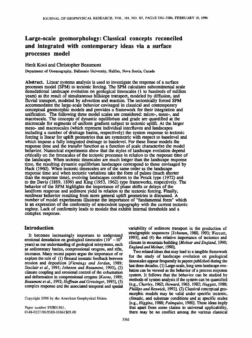
Figure 4. Large-scale, integrated model response to a step change in v• measured by the ratio of the total sediment flux •s that exits the model to the the total tectonic influx d• T of material through its base. Results are shown for experiment M2 and for several cases in which either the scale or one of the controls has been modified with respect to M2 as described in the text. The response curves approximately obey (12), demonstrating linear behavior of the macroscale model system. Note that the timescale is 0-300 m.y. for the spatial scale x10 experiment.

steady state concept can only be applied to mean behavior at geological timescales.

Response to a Step Change in Tectonic Uplift Rate: Linear Behavior

Response time of macroscale landscapes. M2 is an example of a model in which the landscape evolves in response to a step change in v• (Figure 3). For t < 0, v• = 0 and the landscape is a flat surface with low amplitude white noise topography. For t > 0, v• > 0 and the landform evolves from the initial steady state to another [e.g., Willgoose, 1994a]. The change is rapid at first then progressively slows as the steady state is approached.

Figure 4 illustrates the integrated model response measured by the ratio of the total sediment mass flux •s that exits the model to the the total tectonic influx of material

through its base d• T, i.e., the integral of v• over the uplifting region. The step response of M2 is exponential in form (Figure 4) which implies that despite the complexities of behavior as a function of scale the whole system evolves at a rate proportional to its disequilibrium. That is,

(12)

the mesoscale an interfluve achieves a steady state form when its elevation changes at the same rate that the adjacent streams incise (the dynamic equilibrium of Ahnert [1987b]).

A trivial steady state landscape is the flat surface at baselevel [Willgoose et al., 1991a]. It occurs when the tectonic uplift rate and the rate of baselevel fall are zero everywhere in the model domain and this state is independent of the other external controls. This flat surface is the model planation surface or ultimate plain [Chorley et al., 1973, p. 190].

Equifinality. All steady state model landscapes, apart from the flat surface, depend on the initial topography. It determines the initial drainage network which subsequenfiy evolves to steady state by divide migration and drainage capture. Drainage capture is generally necessary because the drainage net must be fully integrated and connected to baselevel before the steady state landscape can be achieved. Details of the ultimate drainage network and the exact location of channels and interfluves in the steady state landscape reflect differences in the initial model topography and drainage net. Model experiments show that for a given tectonic uplift rate, climate, boundary conditions and substrate a suite of landscapes exist that satisfy the condition of steady state. The topography of M2 (Figure 3), for example, is not symmetric with respect to a vertical plane perpendicular to the main drainage divide, even though its external controls are symmetric. The mirror image of the model is another steady state landscape for the same external controls.

The suite of models may have morphomeu'ic characteristics in common [see also .rioward 1994]. If so, the concept of equilreality should be applied to these statistical properties. An additional point is that steady states exist only when the external controls do not vary with time. Short- period fluctuations occur in natural systems, therefore the

where • is the response time, the time taken to reduce the disequilibrium to 1/e times the initial disequilibrium (similar to Howard's [1982] relaxation time). The response time is independent of the magnitude of the step change in uplift rate. An equivalent exponential "relaxation" response is also given when M2 is first brought to a steady state with constant v•,, and v•, is subsequently set to zero. The relaxation response time is the same as the response time for a step function increase in v•,, as expected for systems governed by equations of the form of (12).

Figure 4 also illustrates the same measures of the system response when (1) the precipitation rate in the model is doubled, (2) substrate detaches more easily (erosion length scale is halved), (3) isostatic compensation of the denudation is included, and (4) the spatial scale of the model is increased by a factor of 10. The restfits show that the response time is sensitive to climate and substrate, factors that control the efficiency of surface mass transport, and to the spatial scale of the model. Similar conclusions were reached by Ahnert [1987b] for the response time of a single slope subjected to slope wash.

In these experiments the response time is not sensitive to the value of v•, because v• takes the form of tilting slopes and both the diffusive and fluvial transport equations (1) and (2) have a linear slope dependency. The response time remains the same, but the slopes and elevations of the steady state landform and both •!5 r and •s increase in proportion to v•.

Experiments where the wedge-shaped uplift geometry of M2 is replaced by the uniform uplift of a plateau geometry have similar exponential like response curves and characteristic response times. A small deviation in the early evolution corresponds to an initial phase in which the drainage network on the plateau is reorganized into a fully integrated network that drains to baselevel. Ahnert [1987b] found that in similar one-dimensional experiments (he used


a uniform rate of baselevel fall) the response time was a function of the rate of fall. However, his slope wash denudation model had a nonlinear slope dependence. The linear behavior of our model reflects the linearity of the processes when the model geometry does not involve successive large-scale drainage reorganizations and when the substrate conditions are constant•

The effects of tectonic uplift rate, climate, and substrate on the response to a step in tectonic uplift rate are easy to understand, but the effect of isostasy (Figure 4) needs some explanation. Isostasy counteracts the change of surface elevation caused by denudation and tectonic uplift. When tectonic uplift exceeds denudation and topography grows (e.g., Figure 3), isostasy introduces a component of subsidence at a rate proportional to the average surface uplift rate in the absence of isostasy. The converse is also true. The constant of proportionality (p ranges between 0 for an infinitely rigid lithosphere and (p = Pc/Pro for local isostatic compensation, where is the density of the uplifted and/or renuder bedrock •d Pm is the density of the compensating mantle rock. Isostasy, therefore, modifies the effective surface uplift rate and the response time by factors (1- (p) and 1 / (1- (p), respectively. The topography of the steady state landform is not affected by isostasy since, by definition, in steady state the surface elevation is stationary and, consequently, further isostatic adjustment does not occur.

Transfer function. Following standard linear systems analysis, the dynamical behavior of the model system (equation (12)) is best characterized in the frequency domain, where the model response for a general form of tectonic forcing can be decomposed into the responses of the individual spectral components of the forcing function. Fourier transformation of (12) yields

ß $(f)l(i2nf + 1 / •:)I = •r(f)(1 / •), (13)

where •s ( f ) and •T ( f ) are the Fourier transforms of ß s(t) and •r(t), respectively, and f is frequency. The transfer function of (12) is then

H(f ) = •$(f ) / •r(f ) = 1

(14) 1+ i2nf,'

which has amplitude and phase parts (Figure 5)

I 1 IH(t)l = '1 + (2/r•' / tp )2' (15)

arg[H(tp)]= - arctan(2/r•'/tp), (16)

where t t, = 1 / f is the period. Figure 5 illustrates how the model system filters the input •r(tp) to give output •s(tt,). Three domains can be distinguished as follows: (1) tt, >> ,, the sediment flux is in phase with the tecton-ic flux and has the same amplitude; (2) tp << •', the sediment flux is strongly attenuated and delayed by up to tio / 4; and (3) tp -- 2try', the system attenuates the input by approximately a factor of 2 and delays the output by approximately tt, / 8.

Conditions for linear behavior. The linear

macroscale behavior seen in Figure 4 occurs when the

0.8

0.6

0.4

0.2

! I I I I

Phase response

Amplitude response

-80

0 10 20 30 40 50

Figure 5. Transfer function (equation (14)) of (12) describing the linear behavior of the macroscale landscapes for temporal changes in tectonic uplift v• where t• is period and ½' is the response time. Both the amphtude (equation (15)) and phase response (equation (16)) are shown. Three behavioral domains are distinguished as follows: (1) tt,/½'>>l (2) tt,/•:<<l, and (3) tp /t • 2•r.

uplift geometry meets the following conditions: (1) v• is symmetric with respect to baselevel and (2) v•- imposes a fully integrated drainage net which drains all of the topography to baselevel (i.e., it does not contain internal drainage). These conditions follow from the requirement that a linear system must satisfy the principle of superposition. That is, when the model sediment flux evolution for Vr(1) is given by •s(1) and for Vr(2) by q•s(2), then the response to vr(1) + vr(2) is ½s(1) + q•s (2). Superposition requires that the drainage nets of the landforms that are superimposed are the same. In other circumstances, blockages of drainage occur in the constructed landscape and these require some transient period to be removed. Linear model behavior therefore requires that the drainage net is in a steady state throughout the model evolution. This will only occur for the above mentioned conditions.

Quasi-linear behavior occurs when the drainage only requires minor reorganization. A further restriction to the approximately linear behavior is that the tectonic forcing consists only of uplift. Nonlinear behavior for other uplift geometries will be discussed later.

Model M2 and its variations (Figure 4) do not start with a steady state drainage net but, instead, a net created by a white noise topography. The models are, nevertheless, linear because the response time of the drainage net [Willgoose et al., 1991a] to the imposed wedge uplift is much shorter than the response time of the landscape.

Response time of mesoscale landforms. Figure 4 illustrates the quasi-linear scale dependence of the response time of macroscale model landscapes for tectonic uplift and fixed baselevels. The same scale dependence applies for falling baselevels and a reduced or zero uplift rate and, consequently, can be used to analyze the behavior of a model interfluve between two incising streams which control its baselevels. The response time of an interfiuve is always smaller than the response time of the larger macroscale landscape of which it forms a subsystem. Large, fiuvially dominated interfluves have a response time that is roughly proportional to interfluve width (equation


3), whereas small, diffusion-dominated interfluves have a response time that scales approximately as width squared (equation (10)).

Hierarchy of response times. It follows from the space-time linkage that the response time of a landform/landscape is equal to or greater than those of the smaller-scale landform elements that it contains. If the

response times of the macro-, meso-, and microscale model landformsare •:1, •:2 and •:3, respectively, then •:1 > •:2 > •:3. This scaling has important implications for the dynamic states of the respective landforms.

Meso- and Macroscale Model System: Linear Model Behavior for Slow, Intermediate, and Impulsive Tectonic Forcing

Having established that the macroscale model system has a characteristic response time • and transfer function H(t ), the next step is to investigate how the model behavior changes when the timescale of tectonic forcing t v is much longer than the response time, of the same ordtr as the response time, and when the tectonic forcing takes the form of an impulsive event. We interpret these three regimes to correspond to the basic tectonic frameworks envisaged by Hack [1960], Penck [1972] and Davis [1889, 1899] (the cycle of erosion model), respectively, and the model landform behavior is compared with the behavior described by these authors.

Dynamic Equilibrium Landforms, (Hack Framework): The Product of Slow Tectonic Forcing

The transfer function for the linear model system (equations (14)-(16)) shows that when tectonic forcing is slow (t•, >> '1), the input and output fluxes •r(t•,) and ß s(t•) are approximately equal and that there is no significant phase shift or delay in the output with respect to the input. This result means that the model landscapes evolve with time but remain close to the steady state that corresponds to the current tectonic forcing v•, or equivalently, ½r. Were v• to be held constant at its current value, the transient adjustments in the landscapes would be small because the system is close to equilibrium. This evolution through near-equilibrium macroscale landscapes is termed dynamic equilibrium and is equivalent to the behavior of the microscale segments of uniform gradient discussed earlier, which occurs at much shorter timescales because their response time is much less.

Hack [1960, p. 86] envisaged this style of landscape evolution: "... as long as diastrophic forces operate gradually enough so that a balance can be maintained by erosive processes, then the topography will remain in a state of balance even though it may be evolving from one form to another." He refers to these landscapes as being in a state of dynamic equilibrium.

Illustrative model. Figure 6 shows results of model experiment M4 which illustrate the concept of the dynamic equilibrium landscape in the model system. M4 is the same as M2, but instead of an instantaneous increase in tectonic uplift velocity, the velocity accelerates slowly at a constant rate until at 150 m.y. or 25 times the response time, it reaches the uplift velocity employed in M2. Subsequently, the uplift velocity remains constant. Most of the energy in this uplift function is in the range

>> t I , and dynamic equilibrium is reflected by the fact H s keeps close pace with ½T (Figure 6).

Our description of dynamic equilibrium agrees with Strahler [1950], who defines this state to require a balance between opposing forces, such that they operate at equal rates and their effects cancel each other to produce a steady state in which energy is continually entering and leaving the system. The system may evolve, but it must be close to the steady state that corresponds to the current state of the external controls.

Chorley and Beckinsale [1980] describe dynamic equilibrium as a condition in which form oscillates around a stable average value which itself trends continuously through time. This description largely concurs with our definition. However, it is not clear if in their view, the evolving form is close to equilibrium with current controls. Willgoose et al. [1991a] and Ahnert [1987b], for example, use the term dynamic equilibrium to describe a landform that is in a steady state for a constant uplift rate.

The concept of dynamic equilibrium applies equally well to a model system that is controlled by variables other than tectonic uplift (see also Willgoose, [1994a]). Each control has its own response time. It follows that a uniformly uplifted landscape may evolve in a state of dynamic equilibrium in response to long-term changes in climate, flexural rigidity of the lithosphere, baselevel, or a substrate detachability that varies gradually with depth and/or laterally.

Hack [1960] discussed the concept of dynamic equilibrium landscape evolution in the context of the Appalachians. This example poses some problems bemuse the plate convergence that was responsible for the uplift and growth of the Appalachians probably ceased in early Permian time [Pitman and Golovchenko, 1991]. This makes ongoing tectonic uplift in that area unlikely, or if it does occur, the cause is unknown. Moreover, the Appalachians may be considered an old orogen that is approaching planation. In other words, this orogen may be on the tail of the response curve and evolving very slowly.

1.2

• Tectonic • 0.6

;,x f •" Sediment yield •s 0.4

,./., I' 0.0 ...' ..... , .... 0 50 100 150 200 ?.50

Time (My)

Figure 6. Macroscale model response for slow tectonic forcing (experiment M4) measured by the integrated sediment flux H s. The uplift geometry of M2 is used, together with a ramp function of tectonic uplift rate v•, or, equivalently H T, which increases linearly until 150 M.y. or 25•:1, after which it is constant. The maximum uplift rate is the same as in M2. Here H s keeps close pace with H T, indicative of dynamic equilibrium landscapes.


If this is true, it will be exceedingly difficult to distinguish between (1) the "decay to the peneplain (planafion) state" which occurs in the absence of tectonic uplift, (2) a steady state equilibrium that would exist for tectonic uplift that has continued at a constant rate for a long period of time; (3) a "dynamic equilibrium" which occurs for a tectonic uplift rate that varies very slowly, and even (4) a "growth to a steady state landscape state" that would exist when the Appalachians were already reduced to a peneplain in the past and were subsequently subjected to a constant, small uplift rate that has not existed long enough to achieve steady state.

Pitman and Golovchenko [1991] recently made the point that states (2) and (4) might also be produced in the absence of tectonic uplift but, instead, with a constant, slow rate of eustatic sea level fall since the Late

Cretaceous. This suggestion is supported by the behavior of the SPM where as discussed previously, baselevel fall is equivalent to a spatially uniform uplift in the open system behavior.

Dynamic equilibrium of micro- and mesoscale landscape elements. The uniform gradient segments in M4 experience both uniform uplift and tilting which, respectively, have delayed and immediate responses, as explained earlier. Both effects modify the local baselevel of the adjacent higher elevation segment, and, consequently, they initiate a wave of erosion that propagates headward toward the divide. When viewed from the perspective of an observer fixed in the landscape (Eulerian framework), this propagation causes one or more phases of enhanced stream erosion. How long these phases last depends on the signal length scale and its velocity. The immediate and delayed phases of valley incision act as the external controls on the inteffiuves.

It follows that when tectonic uplift geometries are smooth, the timescales of the propagated external controls on the micro- and mesoscale landscape elements are long, perhaps of the same order as the tectonic variations of the macroscale landscape. For these conditions the micro- and mesoscale landscape elements will tend to be in dynamic eqtfilibrium, even when the macroscale landscape is not, because they have smaller response times.

Waxing and Waning Development of Slopes (Penck Framework): The Result of Intermediate Timescale Tectonic Forcing

When tt, • •:•, the model behavior is neither independent of, nor shive to, the tectonic forcing. It is no surprise that this regime posed difficulties to the conceptual modellers.

Penck [1972] argues that the general assumption made by his predecessors, in particular, W.M. Davis, that denudation (exogenetic processes) can be regarded to succeed tectonic uplift (endogenefic processes) is a special case, chosen more for convenience than anything else (or as a pedagogic device (M. Summerfield, personal communication, 1994)). Penck emphasizes that in order to understand erosional landscape evolution, the relationship between the intensity of the endogenefic and exogenefic processes must be considered. He envisaged that tectonic movements commonly involve gradually accelerating uplift from initial quiescence, followed by gradual decelera- tion to final quiescence. Although Penck was aware of the whole range of timescales over which such an uplift cycle

could theoretically be completed (for example, steady state landscapes for constant uplift rates), he believed that intermediate timescales, which we equate with t t, = •l, are most plausible.

Penck [1972] subsequently developed a conceptual model of slope development that remains difficult to understand. The model assumes "slope replacement" created by incision of a stream at the base of the slope. During retreat the lower part of a slope segment is replaced by new slope segments that can have different gradients. As the basal stream incises, it establishes a new slope segment with a gradient that depends on the incision rate of the stream. Penck deduced from his model that (1) when the incision rate is constant (uniform development), the slopes of interfluves develop a uniform gradient and a constant relief (elevation with respect to the stream) (2) when incision accelerates (waxing development), convex upward slope profiles develop and relief increases, and (3) when incision decelerates (waning development), concave upward slope profiles develop and relief declines. Although Penck did not explicitly relate the evolution of incision rate of streams to his tectonic framework, others have attempted this for him in mutually conflicting ways [Chorley et al., 1984, Figure 2.8]. Illustrative model. In model experiment M5 we

investigate the response of the SPM to a Penckian tectonic uplift history (Figure 7). The geometry is the same as M2, but v• takes the form of a cosine with t t, ~ 2•:1. The main result is that the macroscale relief and •ediment yield attain a maximum about 6 m.y. after the uplift rate has reached its peak value. During the interval when the uplift rate is increasing, the relief cannot keep up with the dynamic equilibrium relief (steady state for current uplift rate). Therefore, when the uplift rate is a maximum, a disequilibrium still exists and it takes another 6 m.y., during which uplift rate and dynamic equilibrium relief are already decreasing, before the disequilibrium is removed and the model relief stops increasing. The intersection of the model relief and the dynamic equilibrium relief heralds the onset of decline of the model relief, a phase which continues long after uplift has ceased.

The phases of growth and decay of relief correspond to Penck's [1972] stages of waxing and waning development, respectively. This aspect is brought out most clearly by the cross-sectional evolution displayed in Figure 7. During waxing development the fluvial incision rate is less than the tectonic uplift rate. River gradients therefore steepen, and incision rates increase, continuously striving to achieve equilibrium with the uplift rate. During waning development the converse is true.

The timescales for fluvial incision in M5 are of the

same order as the tectonic uplift timescale. The interfluves are therefore close to a dynamic equilibrium with the incision rates at their bases because their response time is so small that they can easily keep pace with these variations. This explains why during waxing development (when incision rates increase), interfluve relief grows; during uniform development (when the incision rate is constant), interfluve relief is greatest; and during waning development (when the incision rate decreases), interfluve relief declines. A further reduction of t.. would be required for the mesoscale landforms to [xhibit transient (disequilibrium) behavior characterized by phase shifts


between the accelerating or decelerating incision, on the one hand, and interfiuve growth or decline on the other.

The slope morphology for waxing, uniform, and waning development advanced by Penck [1972] is not predicted by the SPM in M5. The model hillslopes stay convex throughout their evolution. This is due to the low spatial resolution of the model and the associated numerical

requirement to scale up the effective diffusivity of hillslope transport [Kooi and Beaumont, 1994]. Diffusive transport and inteffluve convexity therefore occur on larger scales than in natural systems. Higher resolution, less diffusive, one-dimensional model experiments of individual interfluves do exhibit hillslope behavior that is much closer to that envisaged by Penck. Model slopes develop a relatively greater convexity and concavity for accelerating and decelerating incision. To achieve dynamic equilibrium slopes that are straight for a constant incision rate requires the incorporation of smaller-scale processes [e.g., Anderson and Humphrey, 1990].

That the sediment yield from M5 (Figure 7) is out of phase with the tectonic mass input and does not reach the same amplitude follows from the phase and amplitude response of (15) and (16). Equation (16) shows that were tt, even shorter, the delay of the peak sediment yield with respect to the peak uplift rate would be greater than 6 m.y. Correspondingly, were •:1 larger, for example, for model landscapes with a spatial scale of 500 km, peak sediment yield delays of several tens of millions of years would be expecteA. These significant delays are anticipated for natural systems and should be taken into account when using the stratigraphic record to date tectonic events.

Relaxation Landforms, (Davis Framework): The Result of Impulsive Tectonic Forcing

A delta function or pulse of uplift rate v• = •5(t) is used to investigate the model behavior when tectonic forcing takes the form of a rapid event, faster than the response time. The delta function has a white spectrum, meaning that it contains all timescales of uplift rate tt, with equal magnitude.

The assumption of rapid phases of uplift, accompanied by little erosion and separated by prolonged periods of tectonic quiescence, plays a key role in the framework of the classical conceptual work of Davis [1899]. It is particularly this assumption, at least as contained in the "cycle of erosion," that distinguishes his framework from the frameworks of Penck [1972] and Hack [1960] that were discussed in the previous sections.

Illustrative model experiment. Experiment M6 (Figures 8 and 9) illustrates the model impulse response (declining equilibrium of Willgoose [1994a]) for the nearly symmetric uplift geometry used in M2. Figure 8 demonstrates that the impulse response shows an exponential-like decaying evolution. This is expected because for linear systems behavior (equation (12)) the impulse response is the derivative of the step response. Also, the Fourier transform of the impulse response is given by the transfer function (equation (14)) because •T (f) = 1, and (14) is the Fourier wansform of a decaying exponential.

That the M6 sediment flux •s (Figure 8, top fight) shows an initial increase demonstrates that the linear

macroscale model behavior is only an approximation

(compare with Willgoose [1994b]). Initially, before the fluvial system has had much time to incise the average slope of the rivers at baselevel is at a maximum, but the rivers are carrying significantly under capacity because hillslope transport to the valleys is minimal due to lack of relief. Incision and growth of relief progressively enhance hillslope transport to the valleys, the river undercapacity drops, and the sediment yield increases. The Wansifion from growing to declining sediment yield indicates the time when the rivers achieve grade at baselevel for the first time. Subsequently, the sediment yield declines with a response time •:1 that is the same as in M2 because the same substrate and climatic conditions are used. The initially nonlinear systems behavior, which is the result of a finite erosion length scale, occurs when tectonic variations are more rapid than the response time of fiuvially dominated slope elements at baselevel.

The evolution of the model landscape (Figure 8) exhibits many of the characteristics of Davis' [1899] cycle of erosion and is most readily understood by first considering the microscale and then the meso- and macroscales. In the

initial landscape each subsystem is in disequilibrium, even at the microscale, because there are timescale components in the impulsive tectonic uplift or tilting that are shorter than their response time.

The fiuvially dominated microscale segments at the mouths of the major rivers, where discharge is high and response times are smallest (equation (3)), are the first to achieve dynamic equilibrium. Their dynamic equilibrium is equivalent to grade because M6 does not include isostatic compensation. "Grading" of the trunk rivers starts at baselevel and grows progressively headward in a similar way as in the one-dimensional experiment M 1 (Figure 1).

Figure 9 illustrates in a qualitative way how the characteristic evolution of the fiver profile links to the mesoscale inteffluve evolution. At each point along the river profile there is a finite incision rate at t = 0. This rate increases, peaks, and then declines. The transition to decline coincides with the passage of the knickpoint separating the graded (declining) reaches downstream and ungraded (steepening) reaches upstream. Points that are located progressively more upstream experience this transition later and at a slower rate because the kniclc•int declines and its propagation rate decreases (Figure 9). Anderson [1994] describes a similar behavior.

The interfluves are initially in disequilibrium under the step increase in incision rate at t = 0. The denudation rate grows with the characteristic inteffluve response time •:2. The relief of the inteffluves increases, reaches a maximum, and declines when the interfluve denudation rate is, respectively, less, equal to, and greater than the adjacent stream incision rate. The transition from growth to decline in interfluve relief occurs with a phase shift or delay with respect to the peak stream incision rate and is diachronous; that is, it occurs later farther upstream (Figures 8 and 9). The phase lag is the equivalent systems behavior discussed for the macroscale landscape in a Penckian [Penk, 1972] tectonic framework (Figure 8), albeit for smaller timescales.

Downstream, where incision rates are greatest, interfiuves aUain dynamic equilibrium only when incision rates and relief have declined (Figure 9), i.e., significantly after the knickpoint passes. In contrast, upstream, where


..•

..ill J'.::•:: '-'.-... '::-•

":;"' ..::•: '::%:• ::::i]!. ...... ..... 'ii.:....:::..:.• ':.:.:•

':i!.


incision rates are small, dynamic equilibrium may be approximately achieved, even before the incision rate and relief are maximum.

When the interfiuves farthest upstream have achieved dynamic equilibrium, relief declines at all scales. As denudation rates continue to decrease, the macroscale landscape also achieves dynamic equilibrium and, ultimately, steady state when it is worn down to baselevel.

Comparison with Davis' cycle of erosion. The characteristics of the "youth stage" in the cycle of erosion of Davis [1889, 1899] are aggressive, headward cutting, together with vertical incision of the whole drainage network, rapidly increasing (mesoscale) relief, V-shaped valleys, and grading of the major rivers starting at baselevel. The "maturity stage" starts when the interfluve relief reaches a maximum and divides are "narrow."

Throughout maturity, interfluve relief declines while the headward growth of the graded reaches of the drainage network continues. In "old age" all streams, valleyside slopes, and divide crests are graded, and the landscape is composed of broad and gently sloping valleys and rounded divides [Chorley et al., 1984].

In the SPM the same trinity of stages can be recognized. The main difference is that the transition from youth to maturity is diachronous for the reasons explained above and must therefore be defined locally.

For the SPM an alternative, more natural distinction of a trinity of response stages for impulsive tectonic forcing would be (1) transition from stage 1 to stage 2 when all of the microscale landforms have achieved dynamic equilibrium and (2) transition from stage 2 to stage 3 when all of the mesoscale landforms have achieved dynamic equilibrium. These stages can also be recognized for a step change response in uplift rate (experiment M2, Figure 2) and are a general feature of tectonic forcing that includes components at all timescales.

Meso- and Macroscale Model System: Nonlinear Behavior

The approximately linear model behavior described so far occurs for symmetric uplift geometries v• that impose a fully integrated drainage net, draining all of the topography to baselevel. In this section we explore geometrically nonlinear behavior when these conditions do not apply. The analysis is not systematic. Instead, results of a number of model experiments are presented for impulsive tectonic forcing, and the behavior for other temporal tectonic forcing histories is discussed.

Asymmetric Uplift Geometry: Backwearing and Pediplanation [King, 1953,1962] and Importance of Fundamental Form [Brice, 1964]

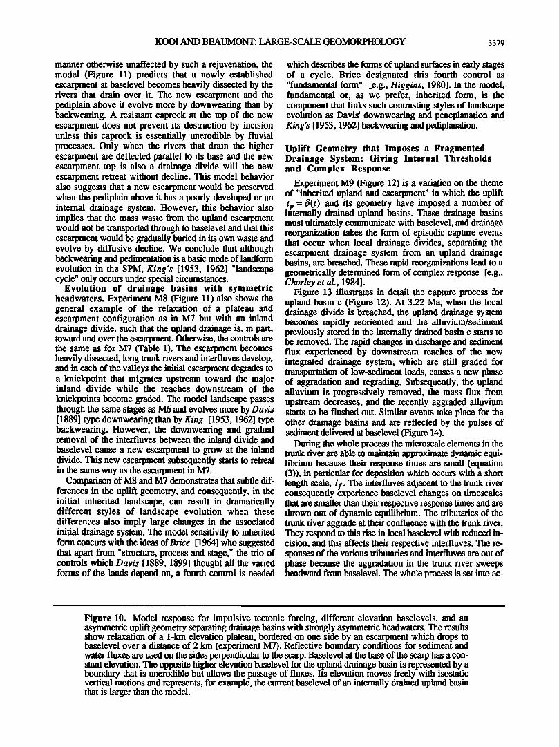
Evolution of drainage basins with strongly asymmetric headwaters. Experiment M7 (Figure 10) illustrates the relaxation from t•, = 6(t) of a plateau bordered on one side by an escarpment. The geometry is a highly asymmetric form of the wedge uplift of M6 with different elevation baselevels. In contrast to the overall

downwearing of topography in M6 (Figure 9), the landscape in M7 decays to a planated state by backwearing or retreat of the initial escarpment and planation below the escarpment [Kooi and Beaumont, 1994]. The planation surface consists of very low interfluves that separate graded rivers which drain at a low gradient from the foot of the escarpment to baselevel.

Both the backwearing of the escarpmem and the creation of a low-gradient planation surface at its base describe the basic characteristics of the classical conceptual model of landform evolution of King [1953, 1962]. This evolution also agrees with the conceptual ideas of Ollier [1985] for the formation of the "Great Escarpments" on rifted continental margins following rifting of a high-elevation continent [Kooi and Beaumont, 1994; Gilchrist et al., 1994].

An essential condition for model escarpments to retreat in a uniform substrate is that the top of the escarpment be maintained as a drainage divide, separating the plateau drainage basin from the drainage system on and below the escarpment, so that retreat, drainage capture, and divide migration occur in concert. Isostatic uplift [Gilchrist and Summerfield, 1990] helps satisfy this condition because it causes the plateau • tilt away from the escarpment in response to the denudational unloading [Kooi and Beaumont, 1994]. Escarpment retreat in the model is further enhanced when hillslope transport is less efficient than fluvial transport, a condition found in semiarid climate regions or regions which have low weathering rates but significant long-term runoff. This particular climatic control of model escarpment evolution is compatible with the fact that King's [1953, 1962] ideas were strongly influenced by the landscapes of southern Africa, which appear to match these conditions.

However, other experiments show that the SPM does not support King's [1953, 1962] notion that a second pulse of relative baselevel fall causes a new scarp to form, recede, and consume the older pediplain above it. In contrast to King, who thought that the upland above the new escarpment would evolve at a higher elevation but in a

Figure 7. Model response for intermediate tectonic forcing (experiment M5). Tectonic forcing •T, normalized b?L•_ts maximum value, consists of (l+cos2n't/•;1)• -ax/2, where •;1 is the response time. Here •• and the geometry are the same as those in M2. Landscape evolution (middle) shows increasing and declining__topography and relief. The corresponding integrated sediment flux evolution, •s, normalized by •/•, is shown as top fight. Dots indicate the current value of the tectonic forcing function. Mesoscale topographic evolution for cross-section AA' (middle) is shown at bottom left for the same times displayed in the landscape evolution. The phases of growing (waxing) and declining (waning) relief are shown separately.



.< I !


•7

..

.

..

o

II


manner otherwise unaffected by such a rejuvenation, the model (Figure 11) predicts that a newly established escarpment at baselevel becomes heavily dissected by the rivers that drain over it. The new escarpment and the pediplain above it evolve more by downwearing than by backwearing. A resistant caprock at the top of the new escarpment does not prevent its destruction by incision unless this caprock is essentially unerodible by fluvial processes. Only when the rivers that drain the higher escarpment are deflected parallel to its base and the new escarpment top is also a drainage divide will the new escarpment retreat without decline. This model behavior also suggests that a new escarpment would be preserved when the periplain above it has a poorly developed or an internal drainage system. However, this behavior also implies that the mass waste from the upland escarpment would not be transported through to baselevel and that this escarpment would be gradually buried in its own waste and evolve by diffusive decline. We conclude that although backwearing and pedimentation is a basic mode of landform evolution in the SPM, King's [1953, 1962] "landscape cycle" only occurs under special circumstances.

Evolution of drainage basins with symmetric headwaters. Experiment M8 (Figure 11) also shows the general example of the relaxation of a plateau and escarpment configuration as in M7 but with an inland drainage divide, such that the upland drainage is, in part, toward and over the escarpment. Otherwise, the controls are the same as for M7 (Table 1). The escarpment becomes heavily dissected, long trunk rivers and interfluves develop, and in each of the valleys the initial escarpmem degrades to a knickpoint that migrates upstream toward the major inland divide while the reaches downstream of the

knickpoints become graded. The model landscape passes through the same stages as M6 and evolves more by Davis [1889] type downwearing than by King [1953, 1962] type backwearing. However, the downwearing and gradual removal of the interfluves between the inland divide and

baselevel cause a new escarpment to grow at the inland divide. This new escarpment subsequently starts to retreat in the same way as the escarpment in M7.

Comparison of M8 and M7 demonstrates that subtle differences in the uplift geometry, and consequently, in the initial inherited landscape, can result in dramatically different styles of landscape evolution when these differences also imply large changes in the associated initial drainage system. The model sensitivity to inherited form concurs with the ideas orBrice [1964] who suggested that apart from "structure, process and stage," the trio of controls which Davis [1889, 1899] thought all the varied forms of the lands depend on, a fourth control is needed

which describes the forms of upland surfaces in early stages of a cycle. Brice designated this fourth control as "fundamental form" [e.g., Higgins, 1980]. In the model, fundamental or, as we prefer, inherited form, is the component that links such contrasting styles of landscape evolution as Davis' downwearing and peneplanafion and King's [1953, 1962] backwearing and pediplanation.

Uplift Geometry that Imposes a Fragmented Drainage System' Giving Internal Thresholds and Complex Response

Experiment M9 (Figure 12) is a variation on the theme of "inherited upland and escarpment" in which the uplift tt, = 6(t) and its geometry have imposed a number of internally drained upland basins. These drainage basins must ultimately communicate with baselevel, and drainage reorganization takes the form of episodic capture events that occur when local drainage divides, separating the escarpment drainage system from an upland drainage basins, are breached. These rapid reorganizations lead to a geometrically determined form of complex response [e.g., Chorley et al., 1984].

Figure 13 illustrates in detail the capture process for upland basin c (Figure 12). At 3.22 Ma, when the local drainage divide is breached, the upland drainage system becomes rapidly reoriented and the alluvium/sediment previously stored in the internally drained basin c starts to be removed. The rapid changes in discharge and sediment flux experienced by downstream reaches of the now integrated drainage system, which are still graded for transportation of low-sediment loads, causes a new phase of aggradation and regrading. Subsequently, the upland alluvium is progressively removed, the mass flux from upstream decreases, and the recently aggraded alluvium starts to be flushed out. Similar events take place for the other drainage basins and are reflected by the pulses of sediment delivered at baselevel (Figure 14).

During the whole process the microscale elements in the trunk fiver are able to maintain approximate dynamic equilibrium because their response times are small (equation (3)), in particular for deposition which occurs with a short length scale, lf. The interfluves adjacent to the trunk fiver consequently experience baselevel changes on timescales that are smaller than their respective response times and are thrown out of dynamic equilibrium. The tributaries of the trunk fiver aggrade at their confluence with the trunk fiver. They respond to this rise in local baselevel with reduced incision, and this affects their respective interfluves. The responses of the various tributaries and interfluves are out of phase because the aggradation in the trunk fiver sweeps headward from baselevel. The whole process is set into ac-

Figure 10. Model response for impulsive tectonic forcing, different elevation baselevels, and an asymmetric uplift geometry separating drainage basins with strongly asymmetric headwaters. The results show relaxation of a 1-kin elevation plateau, bordered on one side by an escarpment which drops to baselevel over a distance of 2 km (experiment M7). Reflective boundary conditions for sediment and water fluxes are used on the sides perpendicular to the scarp. Baselevel at the base of the scarp has a constant elevation. The opposite higher elevation baselevel for the upland drainage basin is represented by a boundary that is unerodible but allows the passage of fluxes. Its elevation moves freely with isostatic vertical motions and represents, for example, the current baselevel of an internally drained upland basin that is larger than the model.


qlmll


Table 1. Model Parameter Values

Parameter Value

Experiments M2 to M6

,••f (bedro,•k) •sediment) •'R

ir 0tock) • (sediment) ./IS (M3 vertical ridge) If (M3 vertical ridge)

_K•y (bedrøck) (sediment)

(bedrock)

/• (s•em)

O. 2 m 2 / yr 2.0m 2/yr O. 01m/ yr 100 km 1 km 0. 02 m2 / yr 1000 km

Experiments M7 to M9

O. 5 m 2 / yr 5.0m 2/yr O. 01m/ yr 100 km 1 km 30/on

K s is diffusivity; KfV R is a measure of the fluvial sediment carrying capacity as a result of precipitation, V R;

[ofl erodibility length scale; T e, effective elastic thickness flexural calculations.

tion without external forcing at the moment of capture and therefore corresponds to an intemal threshold.

These examples demonstrate nonlinear response from the geometry of tectonic uplift. Corresponding examples of complex model response are also seen for nonuniform substrates and for extrinsic forcing by climate and sea level.

Incompatibility of Form' Giving Internal Thresholds and Complex Response

The geometrically complex response of the models can be described in a wider context. Experiment M9, for example, illustrates complex response for an uplift geometry that imposes a drainage system which includes internal drainage and impulsive tectonic forcing. However, a complex response also occurs in M9 for slow and intermediate tectonic forcing. In general, a geometrical complex response will occur for any uplift geometry that does not impose a fury integrated drainage system that communicates with baselevel; this response occurs irrespective of the time dependence of tectonic forcing. This is so because model landscapes evolve toward the steady state for the current uplift rate and the steady state landscapes require a fully integrated drainage system. Internal drainage basins can achieve no balance between tectonic mass input and denudational mass output. This is a metastable state, and it must be resolved through drainage capture and the complex response.

The remaining class of uplift geometries to be discussed is that in which they are asymmetric yet impose a fury integrated drainage net. Their behavior also includes drainage reorganization, particularly when the uplift is strongly asymmetric and the primary drainage divide is not at a steady state location. For example, in a strongly asymmetric version of the wedge uplift used in M2 to M6 the steady state primary divide does not coincide with the locus of maximum uplift rate. It is, instead, displaced toward the center of the model and the divide will migrate

in this direction. The displacement increases with the asymmetry of the uplift geometry and is independent of the uplift rate.

Consider, for example, that steady state in this asymmetric type of model has been achieved and that the uplift subsequently accelerates. When the acceleration occurs slowly, the drainage net may remain in near steady state while elevations grow. In contrast, when uplift occurs fast enough to impose the tectonic geometry on the landscape, a new divide is created and an internal drainage basin is formed. This internal basin will, when the acceleration decreases below a certain threshold value, be captured by breaching of the new drainage divide, resulting in a complex response. Similar complex behavior can be envisaged for other temporal changes in the uplift geometry.

We regard the importance of the uplift geometry in gov- erning the style of model behavior as a more general statement of Brice's [1964] fundamental form. Hence the role of fundamental (inherited) form is interpreted as an expression of the degree of conformity of antecedent topography with the new tectonic geometry. Nonconformity, in particular of antecedent and imposed drainage patterns, causes the geometrical complex response.

Discussion and Conclusions

In this paper we have undertaken a systematic analysis of the behavior of a SPM for tectonic forcing using a number of systems analysis techniques. This analysis indicates concordance between the model results and a broad

range of geomorphic concepts and styles of behavior envisaged in classical and more contemporary geomorphic models concerning large-scale, long-term landform evolution. These concepts and models include the role of baselevels, grade, steady state equilibrium landforms, Davis [1889,1899] type (downwearing peneplanation), Penck [1972] type (waxing and waning development), and King [1953, 1962] type (escarpment retreat, pediplanation) landscape evolution, Hack [1960] type dynamic equilibrium, response times, and geometrical complex response. The key factors that control the integration of these concepts in the model framework are the nature of the tectonic uplift geometry and its timescales. Despite this integration of behavioral characteristics the results prove neither that the SPM nor the characteristic behavior accord

with natural landscapes. Figure 15 illustrates schematically that the styles of

landform evolution envisaged by Davis [1889, 1899], Penck [1972], and Hack [1960] correspond to subdomains of the behavior of the SPM when it behaves linearly. Hack's dynamic equilibrium landforms occur for t•, >> and are characterized by a dynamic equilibrium state at all spatial scales. Landform evolution envisaged by Penck corresponds to values of t.. that are of the order of ,• or 1 • .

'2. The macroscale landscape •s therefore •n a transient (disequilibrium) state, and either the microscale ( or both the micro- and mesoscale ( •'p -- •'2) landforms are in dynamic equilibrium. Penck's description of slope development concentrated in particular on ,•, -- '2. Davis' decaying landforms following impulsive tectonic forcing evolve through the complete range of model states. These states start with transient landforms at all scales, after


z


3.20 m.). 3.22 m.y. 3.30 m.y. alluvium

3.48 m.y. . ..-;-'.:•. ...... 1.5.,........•:..:::..::...•...i... •_•...•.•,

'•..::...":.-":.-.'..: ::i ,; .:-•. •"..• ....... !":•:. :::.:i:

.•'•;.?.:-;-;;. ::-:-.• -...:...; ::.::.....-;..;::-:-, .: '•: .-..-. ::..--....•::: -½-?"-,-":".;.i..::::½ ......... ;..' ;::'.::;".?-..:':/'":(' ;.'-:-".,'."

Figure 13. Detailed illustration of the capture of upland drainage basin c and the resulting complex response of the trunk fiver. (See Figure 12 for location of the area displayed.) Lines indicate the drainage net. Light and dark shading denote alluvium and bedrock substrate, respectively.

which progressively larger landform elements achieve dynamic equilibrium (in a diachronous way), until, ultimately, the entire landscape approaches the steady state peneplain.

It is not surprising that the cyclic and historical conceptual models of Davis [1889, 1899] and Penck [1972] correspond to conditions for which the SPM behaves linearly. Cyclic refers to the characteristic that both the tectonic forcing and the landforms evolve through patterns that are recurrent, and historical implies that within each cycle the landforms evolve through characteristic stages that are readily predictable as a function of time, or at least, form a progression.

The deterministic nature of these conceptual models is compatible with linear systems behavior for cyclic forcing. However, the SPM also demonstrated the importance of

5

3 $ 2

aggradation and regrading flushing out of aggraded

of major river % alluvium

capture of inland drainage basin

i ' I ' I ß I ' I ' i ß I ' I ß 0 2 4 6 8

Time (My) Figure 14. Integrated sediment flux ½s of M9 (Figure 12).

response time in determining phase shifts or delays and attenuation in the landform response and sediment yield in relation to the tectonic forcing. The current landscape and sediment yield is shown to be a function of both the current and past tectonic forcing in which the "memory" or "inertia" of the landscape is measured by its response time. Tectonic forcing at timescales shorter than the macroscale response time (t/, < a:l) can therefore lead to a palimpsest of landforms which retain information about the history of the external controls [Brunsden and Thornes, 1979].

The behavior of the SPM suggests that the cyclic and historical nature of the geomorphic system disappears for uplift geometries that lead to nonlinear behavior. Only for special simple conditions that cause incremental divide migration and drainage capture, such as King [1953, 1962] type escarpment retreat, can the historical approach be of some use.

Further analysis is required to investigate the model behavior for other model controls, such as climate and substrate conditions, and to explore more extensively the effect of geometrical nonlinearities. Also of interest is the effect that nonlinear fluvial transport formulations might have on the model behavior. Apart from the geomorphic concepts discussed in this paper it is important to relate empirical relationships, such as those between denudation rate and local relief, and area and slope in drainage networks to the equivalent model statistics [e.g., Willgoose et al., 1991c; Willgoose, 1994a]. In particular, the search for model statistics that may discriminate between different states of landscape evolution (steady state, dynamic equilibrium, transient) is very valuable [Willgoose, 1994b]. However, the problem remains that the states of natural landscapes have to be known first in order to validate the model statistics.

The richness and complexity of the model behavior may be enhanced when other processes, omitted in this formulation, are incorporated or when the modeled


Integration of classical conceptual models in a systems framework

Davis ,

Penck Hack

MACRO SCALE

MESO SCALE

MICRO SCALE EQUILIBR. EQUILIBR.

I q•l

STEADY

STEADY

STEADY

Figure 15. Schematic illustration of the possible model states for linear model behavior expressed in terms of wansient (disequilibrium), dynamic equilibrium, and steady state equilibrium states for micro-, meso-, and macroscale landforms as a function of the timescale of tectonic forcing t.. The styles of landform evolution envisaged by Davis [1889, 1899], Penck [1972] and Hack [19•0] are shown to correspond to subdomains of the behavior of the surface processes model. The continuum of model system states reflects the importance of space-time linkage.

transport processes are subdivided into their component processes, an approach required to model small-scale landforms. We believe, however, that the unifying power of this simple model demonstrates that the two modes of mass transport capture the essence of the natural system. In particular, the reaction component in the fluvial transport or an equivalent formulation is required to account for the effects of bedrock lithologies in cyclic time.

Appendix: Response of a Uniform Gradient Segment Fluvial Transport

For the uniform gradient "river" segment, length Al, (1) becomes

I -Kf Al VE =-•f qr - qf + VT, (A1)

with the various terms defined in Figure 1, and VE = Oh/& is the dependent variable. Multiplying by -1, adding v•, and dividing by Al gives

c}S 1 V T V•

•--• = Al(lf ) (-KfqrS - qf )- • + -- (A2) Al'

where S = (h'- h) / Al is the gradient of the segment. Separating terms in Syields

t•S K fqr S= q f v T v• (A3) •t + At(If) At(If) At • AI'

A3 is of the general form

ø30 k I (A4) o•t •:

which is a first-order linear differential equation that describes the relationship between the input I and output 0 of a linear filter with response time •:. Therefore the uniform gradient segment behaves as a linear system with respect to temporal forcing by qs, VT and vI, and adjusts its slope S with response time • = At{It •/Kfq r. Note that because the response time d•pends 6fithe dbtachability If of the substrate, it is much shorter for deposition than defiuclation of resistant bedrock.

Hillslope Diffusive Transport

Following the same procedure for (2) yields

1 _K s - qs + VT' VE = -• AI (As)

Multiplying by -1, adding v•, and dividing by Al gives

s= +--' (A6) Al 2 Al Al

which is also of the linear form (A4) with •:• = 312 / Ks. As expected, diffusive "hillslopes" adjust their slope with the standard diffusive time constant.


Combined Transport

The same procedure for combined transport on a uniform gradient segment yields

JS [ Kfqr + Ks IS= qf qs VT '•+ Al(lf ) A/2 J At(If) At 2 At Al

d The from which one obtains 1 / •:us = 1 / •:• + 1 / •:us. response time for the combined transport tends to that of the fastest process. The combined response time takes this form because the processes act in parallel. It also explains why fluvial processes (which scale with At{lj•) ) dominate at large scales (i.e., are lo•ng range), wherea•-diffusive processes (which scale as Al z ) may dominate at small scales (i.e., short range) when If is finite.

Acknowledgments. This work was funded by an NSERC Research Grant to C.B., and during part of this work, H.K. was supported by a Dalhousie University Killam Postdoctoral Fellowship. The work benefited from corntractive discussiota with Alan Gilchrist, Mike Summerfield, Peter Molnar, and Philippe Fullsack, and we thank Juliet Hamilton and Tammy Chouinard for help in producing the manuscript. We also thank Mike Summerfield and Bob Anderson for their critiques and assistance in penetrating geomorphic terminology and Greg Tucker and Gary Willgoose for additional comments.

References

Altoeft, F., Brief description of a comprehensive three-dimensional process response model for landform development, Z. Geomorphol., Suppl. 25, 2949, 1976.

Ahnert, F., Process respome models of denudation at different spatial scales, in Geornorphological Models: Theoretical and Empirical Aspects, edited by F. Ahnert, Catena Suppl., 10, 31-50, 1987a.

Altoeft, F., Approaches to dynamic equilibrium in theoretical simulatiom of slope development, Earth Surf. Processes Landforms, 12, 3-15, 1987b.

Anderson, R.S., Evolution of the Santa Cruz Mountaim, California, through tectonic growth and geomorphic decay, J. Geophys. Res., 99, 20,161-20,180, 1994.

Anderson, R.S., and N.F. Humphrey, Interaction of weathering and transport processes in the evolution of arid landscapes, in Quantitative Dynamic Stratigraphy, edited by T.A. Cross, pp. 349-361, Prentice-Hall, Englewood Cliffs, N.J., 1990.

Beaumont, C., P. Fullsack, and J. Hamilton, Erosional control of active compressional orogens, in Thrust Tectonics, edited by K.R. McClay, pp. 1-18, Chapman and Hall, New York, 1992.

Brice, J.C., Fourth genetic factor for sculptural relief, Spec. Pap. Geol. Soc. Am., 82, 1964.

Brimsden, D., and J. Thornes, Landscape semitivity and change, Trans. Inst. Brit. Geogr., 4, 463-484, 1979.

Carslaw, H.S., and J.C. Jaeger, Conduction of Heat in Solids, Clarendon, Oxford, 1959.

Chase, C.G., Fluvial landsculpting and the fractal dimemion of topography, Geornorphology, 5, 39-57, 1992.

Chorley, R.J., Geomorphology and general systems theory,

U.S. Geol. Surv. •r•f. Pap., 500-B, 1962. Chorley, R.J., and . . Beckinsale, G.K. Gilbert's geomorphology, Spec. Pap. Geol. Soc. Am., 183, 129-142, 1980.

Chorley, R.J., R.P. Beckimale, and A.J. Dunn, The History of the Study of Landforms or the Development of Geomorphology, v.2, The Life and Work of William Morris Davis, 874 pp., Methuen, New York, 1973.

Chorley, R.J., S.A. Schumm, and D.E. Sugden, Geomorphology, 390 pp., Methuen, New York, 1984.

Culling, W.E.H., Theory of erosion of soil-covered slopes, J. Geol., 73, 230-254, 1965.

Davis, W.M., The rivers and valleys of Pennsylvania, Nat. Geogr. Mag., I, 183-253, 1889.

Davis, W.M., The geographical cycle, Geogr. J., 14, 481- 504, 1899.

England, P., and P. Molnar, Surface uplift, uplift of rocks, and exhumation of rocks, Geology, 18, 1173-1177, 1990.

Flemings, P.B., and T.E. Jordan, A synthetic stratigraphic model of foreland basin development, J. Geophys. Res., 94, 3851-3866, 1989.

Gilbert, G.K., Report on the Geology of the Henry Mountains, 160 pp., Rocky Mountain Region, U.S. Geol. Surv., Denver, Colorado 1877.

Gilchrist, A.R., and M.A. Summerfield, Differential denudation and flexural isostasy in the formation of rifted-margin upwarps, Nature, 346, 739-742, 1990.

Gilchrist, A.R., H. Kooi, and C. Beaumont, The post- Gondwana geomorphic evolution of south-western Africa: Qualitative comparison of observatiom with a numerical model, J. Geophys. Res., 99, 12,211-12,228, 1994.

Hack, T.J., Interpretation of erosional topography in humid temperate regiom, Am. J. Sci., 258A, 80-97, 1960.

Higgins, C.G., Theories of landscape development, a perspec- five, in Theories of Landform Development, edited by W.N. Melhorn and R.C. Flemal, pp. 1-28, Allen and Unwin, Winchester, Mass., 1980.

Hoffman, P.F., and J.P. Grotzinger, Orographic precipitation, erosional unloading, and tectonic style, Geology, 21, 195- 198, 1993.

Howard, A.D., Geomorphological systems - Equilibrium and dynamics, Am. J. Sci., 263, 305-312, 1965.

Howard, A.D., Equilibrium and timescales in geomorphology: Application to sand-bed alluvial streams, Earth Surf. Processes Landforms, 7, 303-325, 1982.

Howard, A.D., A detachment-limited model of drainage basin evolution, Water Resour. Res., 30, 2261-2285, 1994.

Howard, A.D., W.E. Dietrich, and M.A. Seidl, Modeling fluvial erosion on regional to continental scales, J. Geophys. Res., 99, 13,971-13,986, 1994.

Huggert, R.J., Dissipative systems' Implications for geomorphology, Earth Surf. Processes Landforms, 13, 45-49, 1988.

Johnson, D.D., and C. Beaumont, Preliminary results from a planform kinematic model of orogen evolution, surface processes and the development of clastic foreland basin stratigraphy, Spec. Publ. Soc. Econ. Paleontol. Mineral., 52, 3-24, 1995.

King, L.C., Cannom of landscape evolution, Geol. Soc. Am. Bull., 64, 721-752, 1953.

King, L.C., The Morphology of the Earth, 699 pp., Oliver and Boyd, Edinburgh, 1962.

Kirkby, M.J., A two-dimemional simulation model for slope and stream evolution, in Hillslope Processes, edited by A.D. Abrahams, pp. 203-222, Allen and Unwin, Winchester, Mass., 1986.

Kooi, H., and C. Beaumont, Escarpment retreat on high-elevation rifted continental margiro: Insights derived from a surface processes model that combines diffusion, reaction and advection, J. Geophys. Res., 99, 12,191-12,209, 1994.

Koons, P.O., The topographic evolution of collisional mountain belts: A numerical look at the Southern Alps, New Zealand, Am. J. Sci., 289, 1041-1069, 1989.

Mackin, J.H., Concept of the graded river, Geol. Soc. Am. Bull., 59, 463-512, 1948.

Molnar, P., and P. England, Late Cenozoic uplift of mountain ranges and global climate change: Chicken or egg?, Nature, 346, 29-34, 1990.

Morisawa, M., Rivers, Form and Process, 222 pp., Longman, White Plains, N.Y., 1985.

Ollier, C.D., Morphotectonics of continental margins with great escarpments, in Tectonic Geomorphology, The Binghamton Syrup. in Geomorphol.: lnt. Ser., 15, edited by M. Morisawa and J.T. Hack, pp. 3-25, Allen and Unwin, Winchester, Mass., 1985.

Palmquist, R.C., The compatibility of structure, lithology and


geomorphic models, in Theories of Landform Development, edited by W.N. Melhorn and R.C. Flemal, pp. 145-167, Allen and Unwin, Winchester, Mass., 1980.

Penck, W., Morphological Analysis of Land Forms, a Contribution to Physical Geology, translated from German by H. Czech and K.C. Boswell, 429 pp., Hafner, New York, 1972.

Phillips, J.D., and W.H. Renwick (Ed.), Geomorphic systems, Geomorphology,$, 195-491, 1992.

Pitman IH, W.C., and X. Golovchenko, The effects of sea level changes on the morphology of mountain belts, J. Geophys. Res., 96, 6879-6891, 1991.

Ritter, D.F., Landscape analysis and the search for geomorphic unity, Geol. Soc. Am. Bull., 100, 160-171, 1988.

Rosenbloom, N.A., and R.S. Anderson, Hillslope and channel evolution in a marine terraced landscape, Santa Cruz, California, J. Geophys. Res., 99, 14,013-14,029, 1994.

Schumm, S.A., The Fluvial System, 338 pp., John Wiley, New York, 1977.

Schumm, S.A., Episodic erosion: A modification of the geomorphic cycle, in Theories of Landform Development, edited by W.N. Melhorn and R.C. Flemal, pp. 69-85, Allen and Unwin, Winchester, Mass., 1980.

Schumm, S.A., River response to baselevel change: Implications for sequence stratigraphy, J. Geol., 101, 279- 294, 1993.

Schumrn, S.A., and R.W. Lichty, Time, space and causality in geomorphology, Am. J. Sci.,263, 110-119, 1965.

Seidl, M.A., and W.E. Dietrich, The problem of channel erosion into bedrock, Catena, 23, 101-124, 1992.

Sinclair, H.D., B.J. Coakley, P.A. Allen, and A.B. Watts, Simulation of foreland basin stratigraphy using a diffusion- model of mountain belt uplift and erosion - An example from the central Alps, Switzerland, Tectonics, 10, 599-620, 1991.

Strahler, A.N., Equilibrium theory of erosional slopes approached by frequency distribution analysis, Am. J. Sci., 248, 673-696, 1950.

Tinkler, K.J., A Short History of Geomorphology, 317 pp., Croom Helm, London, 1985.

Tucker, G.E., and R.L. Slingerland, Erosional dynamics, flexural isostasy, and long-lived escarpments: A numerical modeling study, J. Geophys. Res., 99, 12,229-12,243, 1994.

Wescott, W.A., Geomorphic thresholds and complex response of fluvial systems - Some implications for sequence stratigraphy, AAPG Bull., ??, 1208-1218, 1993.

Willgoose, G., A physical explanation for an observed area- slope-elevation relationship for catchrnents with declining relief, Water Resour. Res.,30, 151-159, 1994a.

Willgoose, G., A statistic for testing the elevation characteristics of landscape simulation models, J. Geophys. Res., 99, 13,987-13,996, 1994b.

Willgoose, G., R.L. Bras, and I. Rodriguez-Iturbe, Results from a new model of river basin evolution, Earth Surf. Processes Landforms, 16, 237-254, 1991a.

Willgoose, G., R.L. Bras, and I. Rodriguez-Iturbe, A coupled channel network growth and hillslope evolution model, l, Theory, Water Resour. Res., 27, 1671-1684, 1991b.

Willgoose, G., R.L. Bras, and I. Rodriguez-Iturbe, A physical explanation of an observed link area-slope relationship, Water Resour. Res., 2 ?, 1697-1702, 199 lc.

Willgoose, G., R.L. Bras, and I. Rodriguez-Imrbe, The relationship between catchment and hillslope properties: Explanation of a catchment evolution model, Geomorphology, $, 21-37, 1992.

C. Beaumont and H. Kooi, Department of Oceanography, Dalhousie University, Halifax, Nova Scotia, Canada B3H 4J 1 (e- mail: juliet@wolf. ocean.dal.ca; [email protected])

(Received April 18, 1994; revised June 6, 1995; accepted June 13, 1995.)

Documents

Large&scale geomorphology: Classical concepts reconciled ...geomorphology.sese.asu.edu/Papers/Kooi_and_Beaumont_1996_JGR.pdf · JOURNAL OF GEOPHYSICAL RESEARCH, VOL. tot, NO. B2,