Laser power calculations: sources of error

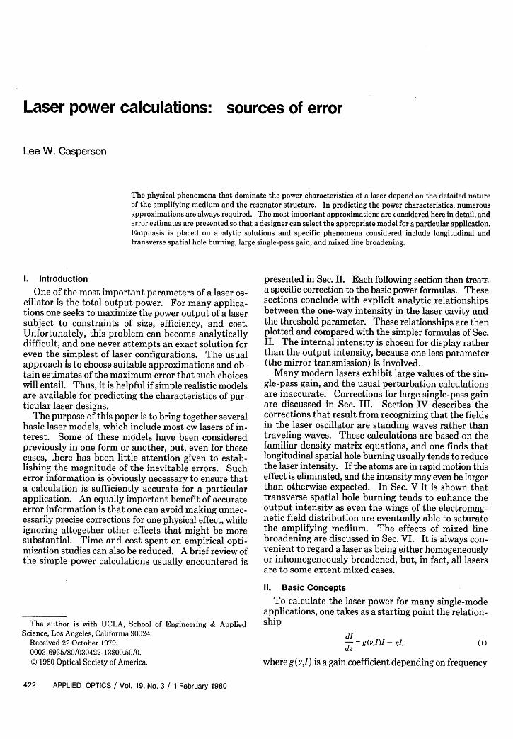
Laser power calculations: sources of error

Lee W. Casperson

The physical phenomena that dominate the power characteristics of a laser depend on the detailed natureof the amplifying medium and the resonator structure. In predicting the power characteristics, numerousapproximations are always required. The most important approximations are considered here in detail, anderror estimates are presented so that a designer can select the appropriate model for a particular application.Emphasis is placed on analytic solutions and specific phenomena considered include longitudinal andtransverse spatial hole burning, large single-pass gain, and mixed line broadening.

1. IntroductionOne of the most important parameters of a laser os-

cillator is the total output power. For many applica-tions one seeks to maximize the power output of a lasersubject to constraints of size, efficiency, and cost.Unfortunately, this problem can become analyticallydifficult, and one never attempts an exact solution foreven the simplest of laser configurations. The usualapproach s to choose suitable approximations and ob-tain estimates of the maximum error that such choiceswill entail. Thus, it is helpful if simple realistic modelsare available for predicting the characteristics of par-ticular laser designs.

The purpose of this paper is to bring together severalbasic laser models, which include most cw lasers of in-terest. Some of these mcidels have been consideredpreviously in one form or another, but, even for thesecases, there has been little attention given to estab-lishing the magnitude of the inevitable errors. Sucherror information is obviously necessary to ensure thata calculation is sufficiently accurate for a particularapplication. An equally important benefit of accurateerror information is that one can avoid making unnec-essarily precise corrections for one physical effect, whileignoring altogether other effects that might be moresubstantial. Time and cost spent on empirical opti-mization studies can also be reduced. A brief review ofthe simple power calculations usually encountered is

The author is with UCLA, School of Engineering & AppliedScience, Los Angeles, California 90024.

Received 22 October 1979.0003-6935/80/030422-13$00.50/0.© 1980 Optical Society of America.

presented in Sec. II. Each following section then treatsa specific correction to the basic power formulas. Thesesections conclude with explicit analytic relationshipsbetween the one-way intensity in the laser cavity andthe threshold parameter. These relationships are thenplotted and compared with the simpler formulas of Sec.II. The internal intensity is chosen for display ratherthan the output intensity, because one less parameter(the mirror transmission) is involved.

Many modern lasers exhibit large values of the sin-gle-pass gain, and the usual perturbation calculationsare inaccurate. Corrections for large single-pass gainare discussed in Sec. III. Section IV describes thecorrections that result from recognizing that the fieldsin the laser oscillator are standing waves rather thantraveling waves. These calculations are based on thefamiliar density matrix equations, and one finds thatlongitudinal spatial hole burning usually tends to reducethe laser intensity. If the atoms are in rapid motion thiseffect is eliminated, and the intensity may even be largerthan otherwise expected. In Sec. V it is shown thattransverse spatial hole burning tends to enhance theoutput intensity as even the wings of the electromag-netic field distribution are eventually able to saturatethe amplifying medium. The effects of mixed linebroadening are discussed in Sec. VI. It is always con-venient to regard a laser as being either homogeneouslyor inhomogeneously broadened, but, in fact, all lasersare to some extent mixed cases.

11. Basic ConceptsTo calculate the laser power for many single-mode

applications, one takes as a starting point the relation-ship

-I= g(,I)I - I,dz

(1)

where g(v,I) is a gain coefficient depending on frequency

422 APPLIED OPTICS / Vol. 19, No. 3 / 1 February 1980

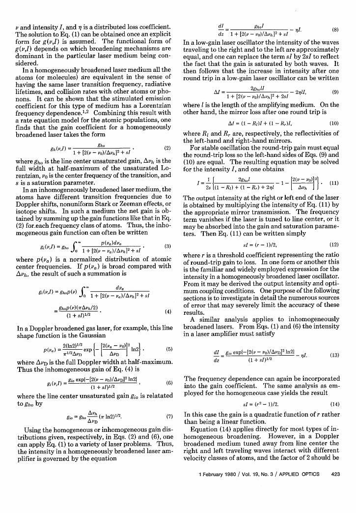
v and intensity I, and -q is a distributed loss coefficient.The solution to Eq. (1) can be obtained once an explicitform for g(vI) is assumed. The functional form ofg(vI) depends on which broadening mechanisms aredominant in the particular laser medium being con-sidered.

In a homogeneously broadened laser medium all theatoms (or molecules) are equivalent in the sense ofhaving the same laser transition frequency, radiativelifetimes, and collision rates with other atoms or pho-nons. It can be shown that the stimulated emissioncoefficient for this type of medium has a Lorentzianfrequency dependence. 1 2 Combining this result witha rate equation model for the atomic populations, onefinds that the gain coefficient for a homogeneouslybroadened laser takes the form

gh (P,I) =gh. 2

1 + [2(v - vO)/Avh2 + sI (2)

where gho is the line center unsaturated gain, Avh is thefull width at half-maximum of the unsaturated Lo-rentzian, vO is the center frequency of the transition, ands is a saturation parameter.

In an inhomogeneously broadened laser medium, theatoms have different transition frequencies due toDoppler shifts, nonuniform Stark or Zeeman effects, orisotope shifts. In such a medium the net gain is ob-tained by summing up the gain functions like that in Eq.(2) for-each frequency class of atoms. Thus, the inho-mogeneous gain function can often be written

gi(VI) = Sho0 1 + [2(v -Va)AVh]2 + sI

where p (vs) is a normalized distribution of atomiccenter frequencies. If p(va) is broad compared withAPh, the result of such a summation is

gi(V,I) = ghp(v) W dvao 1 + [2(v - V,)/Avh]2 + sI

ghP)(7rAVh/2)

(1 + SJ)1/2

In a Doppler broadened gas laser, for example, this lineshape function is the Gaussian

2(1n2)1/2 [_ 2(v,, - po)l2 P(va) = lA exp ln2 J (5)

I112AVDD

where AVD is the full Doppler width at half-maximum.Thus the inhomogeneous gain of Eq. (4) is

gi(vI) = gi, expl-[2(v - Vo)/AVPD]2 ln2} (6)

(1 + SJ)1/2

where the line center unsaturated gain gio is relatatedto gho by

gjo = gho- (r 1n2)1/ 2 . (7)AVD

Using the homogeneous or inhomogeneous gain dis-tributions given, respectively, in Eqs. (2) and (6), onecan apply Eq. (1) to a variety of laser problems. Thus,the intensity in a homogeneously broadened laser am-plifier is governed by the equation

dz 1 + [2(v - vo)/Avh]2 + sI (8)

In a low-gain laser oscillator the intensity of the wavestraveling to the right and to the left are approximatelyequal, and one can replace the term sI by 2sI to reflectthe fact that the gain is saturated by both waves. Itthen follows that the increase in intensity after oneround trip in a low-gain laser oscillator can be written

AI = [2 hol + 2 2=71I,1 + [2(v - vo)/A~h ]

2 + 2s1 I~I(9)

where is the length of the amplifying medium. On theother hand, the mirror loss after one round trip is

AI = (1-R)I + (1 -Rr)I, (10)

where RI and Rr are, respectively, the reflectivities ofthe left-hand and right-hand mirrors.

For stable oscillation the round-trip gain must equalthe round-trip loss so the left-hand sides of Eqs. (9) and(10) are equal. The resulting equation may be solvedfor the intensity I, and one obtains

(11)I 1 | 2gh. l 2(v1 | 2 Vo)1

2s (1 - 11 + (1- R) + 21 L - J~ ,

The output intensity at the right or left end of the laseris obtained by multiplying the intensity of Eq. (11) bythe appropriate mirror transmission. The frequencyterm vanishes if the laser is tuned to line center, or itmay be absorbed into the gain and saturation parame-ters. Then Eq. (11) can be written simply

sI = (r- 1)2, (12)

where r is a threshold coefficient representing the ratioof round-trip gain to loss. In one form or another thisis the familiar and widely employed expression for theintensity in a homogeneously broadened laser oscillator.From it may be derived the output intensity and opti-mum coupling conditions. One purpose of the followingsections is to investigate in detail the numerous sourcesof error that may severely limit the accuracy of theseresults.

A similar analysis applies to inhomogeneouslybroadened lasers. From Eqs. (1) and (6) the intensityin a laser amplifier must satisfy

dI gio expl-[2(v - o)/AVD]2

n2l

dz (1 + sI) 1/2 -II.

(13)

The frequency dependence can again be incorporatedinto the gain coefficient. The same analysis as em-ployed for the homogeneous case yields the result

sI (r2-1)/2. (14)

In this case the gain is a quadratic function of r ratherthan being a linear function.

Equation (14) applies directly for most types of in-homogeneous broadening. However, in a Dopplerbroadened medium tuned away from line center theright and left traveling waves interact with differentvelocity classes of atoms, and the factor of 2 should be

1 February 1980 / Vol. 19, No. 3 / APPLIED OPTICS 423

deleted from Eq. (14). This relative decrease in in-tensity near line center is the familiar Lamb dip, whichis typical of many gas lasers.3

Ill. Large Single-Pass Gain

A. Homogeneously Broadened LasersThe emphasis in Sec. II was on lasers in which the

gain per pass is small compared to unity. It is now ap-propriate to consider in detail the limitations on thevalidity of the low-gain approximation. In a homoge-neously broadened laser, the equations governing theintensity of the wave traveling to the right I+ and theintensity of the wave traveling to the left I- can bewritten4 5

dI+ gh.I+ _ I (15)

dI- -gh.I 16dz 1 + s(I+ + I1 (16)

For simplicity it has been assumed that the laser is op-erating at line center. This assumption does not ac-tually reduce the generality of the analysis, since off-center frequencies can be represented by including aLorentzian frequency factor in the gain and saturationparameters. Also it may be noted here that saturationdepends on the sum of the electric fields rather than onthe intensities, and the resultant longitudinal spatialhole burning is discussed in Sec. IV. However, inhigh-gain lasers the effective standing wave region isshort, and spatial hole burning (which will be found tobe small anyway) can have little effect on the output.

It follows readily from Eqs. (15) and (16) that theproduct of the intensities of the waves traveling to theleft and to the right is a constant independent of z,i.e.,

I+(z)(z) = const. (17)

With a bit more algebra one can find, for example, thatthe intensity incident on the right-hand mirror in ahigh-gain laser with negligible distributed losses is

2sI+(zr) = [(1 - Rr) + (Rr/Ri)/ 2(l - RI)]-1[2h.1 + l(RLRr)].

(18)

In an optimized system the reflectivity of the left-handmirror would, it is hoped, be close to unity, and thus Eq.(18) reduces to

2sI+(zr) = (1 - Rr)(2ghol + nRr). (19)

The threshold parameter is related to the gain and lossby

r = -2ghol/lnRr. (20)

Therefore, Eq. (19) can also be written

-I Zr 9h1

- r 1 ) (21)1 - exp(-2gh.1/r)

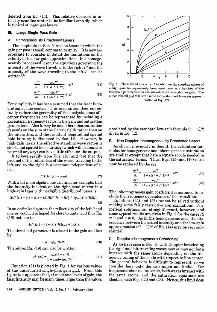
Equation (21) is plotted in Fig. 1 for various valuesof the unsaturated single-pass gain ghol. From thisfigure it is apparent that, at moderate levels of gain, thelaser intensity may be many times larger than the values

10

8

6

sI

4

2

00 2 4 r 6 8 10

Fig. 1. Normalized intensity sI incident on the coupling mirror ofa high-gain homogeneously broadened laser as a function of thethreshold parameter r for various values of the single-pass gain. Thecurve labeled gh,,I = 0 is the same as the standard low-gain approxi-

mation of Eq. (12).

predicted by the standard low-gain formula (r - 1)/2given in Eq. (12).

B. Non-Doppler Inhomogeneously Broadened LasersAs shown previously in Sec. II, the saturation for-

mulas for homogeneous and inhomogeneous saturationare similar except that here a square root is needed inthe saturation terms. Thus, Eqs. (15) and (16) mustnow be replaced by the set

dI+ = gI+ .dz [1 + (I+ + I-)]1/2 '7I

dI - -giI-dz [1 + s(I+ + I-)]1/ + 71T

(22)

(23)

The inhomogeneous gain coefficient is assumed to in-clude the frequency dependence of the transition.

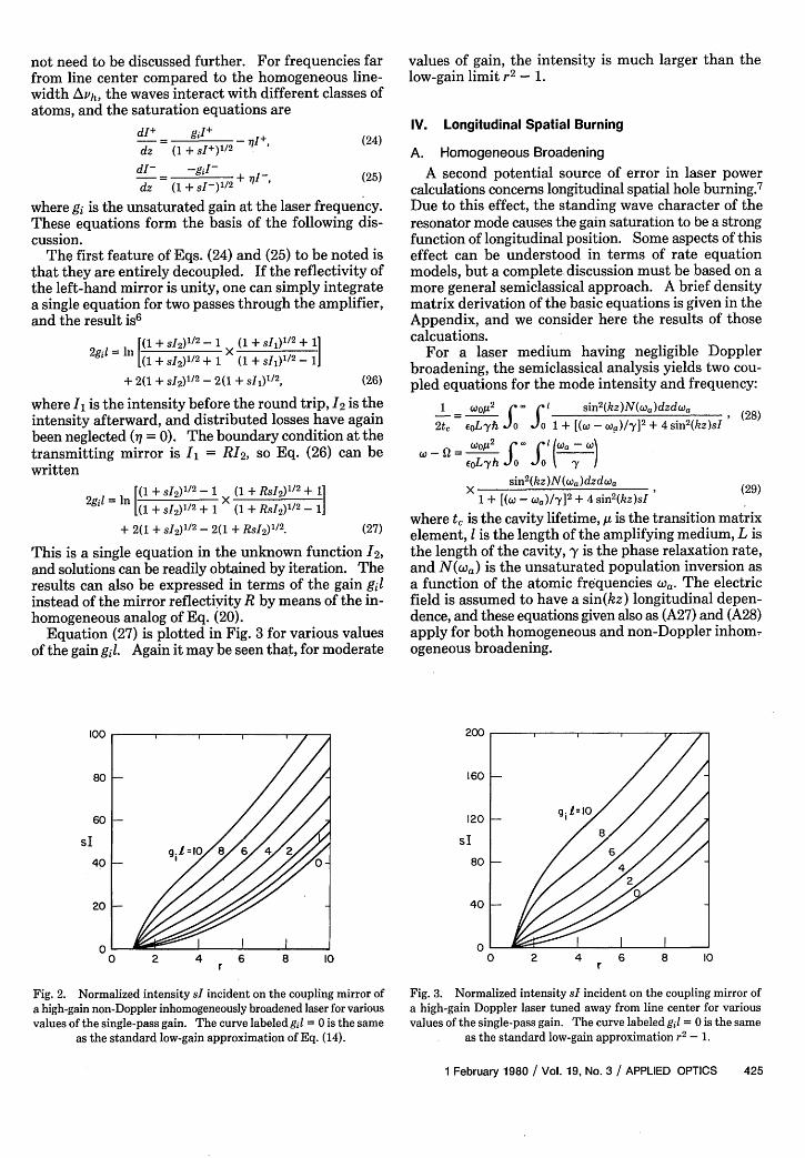
Equations (22) and (23) cannot be solved withoutmaking some fairly restrictive approximations. Nu-merical solutions are straightforward, however, andsome typical results are given in Fig. 2 for the cases Ri= 0 and = 0. As in the homogeneous case, the dis-crepancy between the actual intensity and the low-gainapproximation (r2 - 1)/2 of Eq. (14) may be very sub-stantial.

C. Doppler Inhomogeneous BroadeningAs we have seen in Sec. II, with Doppler broadening

the right and left traveling waves may or may not bothinteract with the same atoms depending on the fre-quency tuning of the mode with respect to line center.The general behavior is difficult to represent, so weconsider here only the two important limits. Forfrequencies close to line center, both waves interact withthe same atoms, and the saturation equations areidentical with Eqs. (22) and (23). Hence, this limit does


not need to be discussed further. For frequencies farfrom line center compared to the homogeneous line-width Avh, the waves interact with different classes ofatoms, and the saturation equations are

dI+ g I2dz (1 + sI+)1/2 - 7I+, (24)

dI- -giI +7I 25

dz (1 + sI-)'1 2 I (25)

where gi is the unsaturated gain at the laser frequency.These equations form the basis of the following dis-cussion.

The first feature of Eqs. (24) and (25) to be noted isthat they are entirely decoupled. If the reflectivity ofthe left-hand mirror is unity, one can simply integratea single equation for two passes through the amplifier,and the result is6

2g~i = n [(1 + SI2)1/2 -1 (1 + sII)1/2

+ 1]

1(1 + I2)1/2 + 1 (1 + SI,) -/2 1

+ 2(1 + sI2)1/2 - 2(1 + sI,)/ 2 , (26)

where I, is the intensity before the round trip, I2 is theintensity afterward, and distributed losses have againbeen neglected (I = 0). The boundary condition at thetransmitting mirror is I = RI 2, so Eq. (26) can bewritten

2gil = n [(1 + SI2) 1/2 X(1 + RsI2 )/2 +

(n + sI 2)1/2 + 1 (1 + RsI2 )12 -11

+ 2(1 + SI2)1/2 - 2(1 + RsI2)12. (27)

This is a single equation in the unknown function I2,and solutions can be readily obtained by iteration. Theresults can also be expressed in terms of the gain gilinstead of the mirror reflectivity R by means of the in-homogeneous analog of Eq. (20).

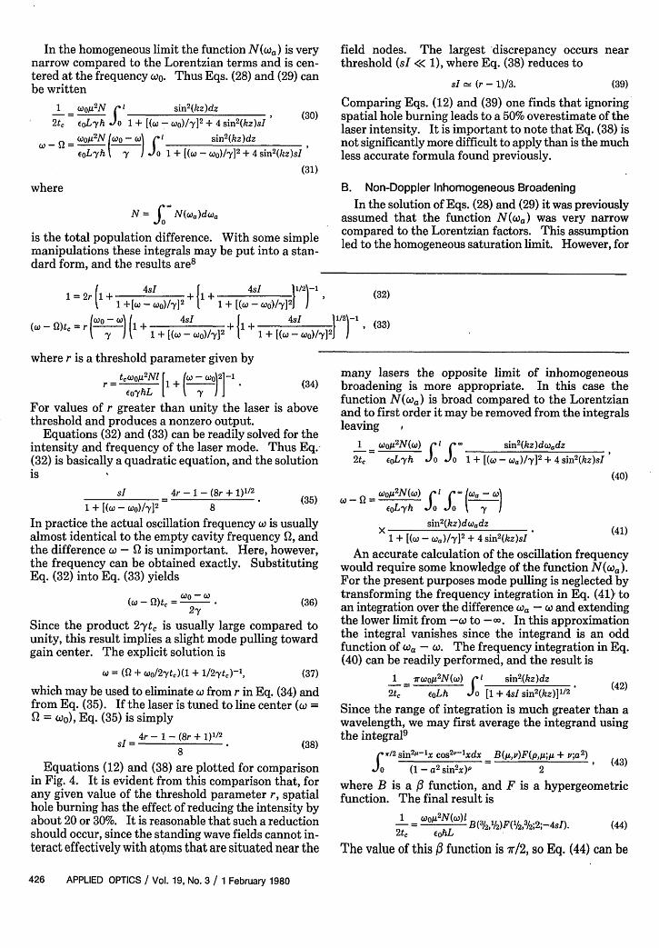
Equation (27) is plotted in Fig. 3 for various valuesof the gain gil. Again it may be seen that, for moderate

100

80-

60

sI

40-

20-

00 2 4 6 8 10

r

Fig. 2. Normalized intensity sI incident on the coupling mirror ofa high-gain non-Doppler inhomogeneously broadened laser for variousvalues of the single-pass gain. The curve labeled gil = 0 is the same

as the standard low-gain approximation of Eq. (14).

values of gain, the intensity is much larger than thelow-gain limit r2

- 1.

IV. Longitudinal Spatial Burning

A. Homogeneous Broadening

A second potential source of error in laser powercalculations concerns longitudinal spatial hole burning. 7

Due to this effect, the standing wave character of theresonator mode causes the gain saturation to be a strongfunction of longitudinal position. Some aspects of thiseffect can be understood in terms of rate equationmodels, but a complete. discussion must be based on amore general semiclassical approach. A brief densitymatrix derivation of the basic equations is given in theAppendix, and we consider here the results of thosecalcuations.

For a laser medium having negligible Dopplerbroadening, the semiclassical analysis yields two cou-pled equations for the mode intensity and frequency:

1 Owa2 fX e' sin2(kz)N(wa)dzda (2

2t, EoLyh Jo Jo 1 + [(W - a)/^y 2 + 4 sin2 (kz)sI

co y SI 0 a wsin2(kz)N(wa)dzdwa ,

1 + [( - Wa)/'y]2 + 4 sin2 (kz)sI

where t, is the cavity lifetime, ,u is the transition matrixelement, is the length of the amplifying medium, L isthe length of the cavity, y is the phase relaxation rate,and N(Wa) is the unsaturated population inversion asa function of the atomic frequencies Da. The electricfield is assumed to have a sin(kz) longitudinal depen-dence, and these equations given also as (A27) and (A28)apply for both homogeneous and non-Doppler inhom-ogeneous broadening.

200

160

120

sI

80

40

00 2 4 6 8 10r

Fig. 3. Normalized intensity sI incident on the coupling mirror ofa high-gain Doppler laser tuned away from line center for variousvalues of the single-pass gain. The curve labeled gil = O is the same

as the standard low-gain approximation r2- 1.


In the homogeneous limit the function N(wa) is verynarrow compared to the Lorentzian terms and is cen-tered at the frequency wo. Thus Eqs. (28) and (29) canbe written

1 Wo5 2N ,IL sin2(kz)dz

2t, EoLyh Jo 1 + [(W -o)/y]2

+ 4 sin2(kz)sI

W - =Wo2 N Wo sin2(kz)dz

coLyh 7 fo 1 + [(W -Wo)/-y] 2 + 4 sin2 (kz)sI

(31)

where

N - N(wa )dw(ha

is the total population difference. With some simplemanipulations these integrals may be put into a stan-dard form, and the results are8

field nodes. The largest discrepancy occurs nearthreshold (sI << 1), where Eq. (38) reduces to

sI (r - 1)/3. (39)

Comparing Eqs. (12) and (39) one finds that ignoringspatial hole burning leads to a 50% overestimate of thelaser intensity. It is important to note that Eq. (38) isnot significantly more difficult to apply than is the muchless accurate formula found previously.

B. Non-Doppler Inhomogeneous BroadeningIn the solution of Eqs. (28) and (29) it was previously

assumed that the function N(coa) was very narrowcompared to the Lorentzian factors. This assumptionled to the homogeneous saturation limit. However, for

12r + 4sI + + 4sI , (32)1 +[W - Wo)/y]

21 1+ [(W - W6)/,y]2

(w-Q)t,=rWO-W (1 + 4sI + 4sI 1/2 - (33)

(z _Il 1 + [(W - o)/y]2

1 + [(W-Wo)/,y]2

where r is a threshold parameter given byI =t'WO

2 Ni [1 + (. - ]o)2J1 . (34)

For values of r greater than unity the laser is abovethreshold and produces a nonzero output.

Equations (32) and (33) can be readily solved for theintensity and frequency of the laser mode. Thus Eq.(32) is basically a quadratic equation, and the solutionis

sI 4r-1-(8r + 1)1 2

1 + 1(w- o)/,y 2 8

In practice the actual oscillation frequency w is usuallyalmost identical to the empty cavity frequency , andthe difference w - is unimportant. Here, however,the frequency can be obtained exactly. SubstitutingEq. (32) into Eq. (33) yields

(W - )t' = (36)

Since the product 2tc is usually large compared tounity, this result implies a slight mode pulling towardgain center. The explicit solution is

w = ( + wo/2yt,)(1 + 1/2yt,)-', (37)

which may be used to eliminate o from r in Eq. (34) andfrom Eq. (35). If the laser is tuned to line center (a =Q = co), Eq. (35) is simply

sI =4r - I - (8r + 1)1/2

8

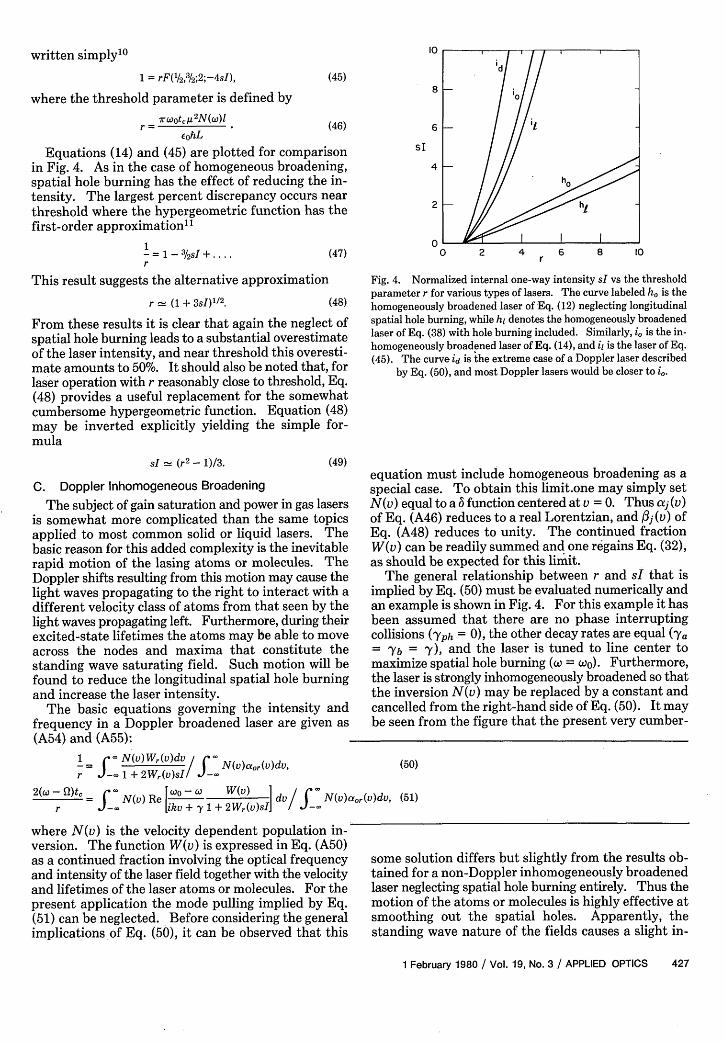
Equations (12) and (38) are plotted for comparisonin Fig. 4. It is evident from this comparison that, forany given value of the threshold parameter r, spatialhole burning has the effect of reducing the intensity byabout 20 or 30%. It is reasonable that such a reductionshould occur, since the standing wave fields cannot in-teract effectively with atoms that are situated near the

many lasers the opposite limit of inhomogeneousbroadening is more appropriate. In this case thefunction N(wa) is broad compared to the Lorentzianand to first order it may be removed from the integralsleaving I

1 wo52N(w) r sin

2(kz)dwadz

2t, coL'yh Jo Jo 1 + [(W - a)/zy]2 + 4 sin2 (kz)sI

(40)

i WOA2Nt°) 4 I feoLyh o o 7

sin2(kz)dwadz

x [c - a )/-y]2 + 4 sin2(kz s(41)

An accurate calculation of the oscillation frequencywould require some knowledge of the function N(coa).For the present purposes mode pulling is neglected bytransforming the frequency integration in Eq. (41) toan integration over the difference Wa - and extendingthe lower limit from -X to -a. In this approximationthe integral vanishes since the integrand is an oddfunction of cOa - co. The frequency integration in Eq.(40) can be readily performed, and the result is

1 =rWosA2 N(w) ' sin2 (kz)dz

2t, coLh Jo [1 + 4sI sin2(kz)]1/2 (42)

Since the range of integration is much greater than awavelength, we may first average the integrand usingthe integral9

/2 sin2

-l1x Cos

2"-lxdx B(5 ,v)F(p,5 ;At + ;a

2)

Jo (1- a2 sin2x)P 2

where B is a : function, and F is a hypergeometricfunction. The final result is

1 Oo2N(W) B(3/ 2,/ 2)F(/ 2,3/;2;-4sI) (44)

2t, cohL

The value of this 3 function is 7r/2, so Eq. (44) can be


written simply1 0

1 = rF(/ 2,3/2 ;2;-4sI),

where the threshold parameter is defined by

7rwOtL2

N(W)I

eohL

where N(v) is the velocity dependent population in-version. The function W(v) is expressed in Eq. (A50)as a continued fraction involving the optical frequencyand intensity of the laser field together with the velocityand lifetimes of the laser atoms or molecules. For thepresent application the mode pulling implied by Eq.(51) can be neglected. Before considering the generalimplications of Eq. (50), it can be observed that this

10

(45)8

(46) 6

sIEquations (14) and (45) are plotted for comparisonin Fig. 4. As in the case of homogeneous broadening,spatial hole burning has the effect of reducing the in-tensity. The largest percent discrepancy occurs nearthreshold where the hypergeometric function has thefirst-order approximation"

1- = 1 -

3/2SI +....-

4

2

0(47)

This result suggests the alternative approximation

r (1 + 3sI)1/2 . (48)

From these results it is clear that again the neglect ofspatial hole burning leads to a substantial overestimateof the laser intensity, and near threshold this overesti-mate amounts to 50%. It should also be noted that, forlaser operation with r reasonably close to threshold, Eq.(48) provides a useful replacement for the somewhatcumbersome hypergeometric function. Equation (48)may be inverted explicitly yielding the simple for-mula

sI (r2 - 1)/3. (49)

C. Doppler Inhomogeneous BroadeningThe subject of gain saturation and power in gas lasers

is somewhat more complicated than the same topicsapplied to most common solid or liquid lasers. Thebasic reason for this added complexity is the inevitablerapid motion of the lasing atoms or molecules. TheDoppler shifts resulting from this motion may cause thelight waves propagating to the right to interact with adifferent velocity class of atoms from that seen by thelight waves propagating left. Furthermore, during theirexcited-state lifetimes the atoms may be able to moveacross the nodes and maxima that constitute thestanding wave saturating field. Such motion will befound to reduce the longitudinal spatial hole burningand increase the laser intensity.

The basic equations governing the intensity andfrequency in a Doppler broadened laser are given as(A54) and (A55):

1 f-N(v)Wr(v)dv/ N(v)ar(v)dv,r 1 + 2W(v)sIl J (-to~~

0 2 4 6 8 10

Fig. 4. Normalized internal one-way intensity sI vs the thresholdparameter r for various types of lasers. The curve labeled ho is thehomogeneously broadened laser of Eq. (12) neglecting longitudinalspatial hole burning, while hi denotes the homogeneously broadenedlaser of Eq. (38) with hole burning included. Similarly, i0 is the in-homogeneously broadened laser of Eq. (14), and il is the laser of Eq.(45). The curve id is the extreme case of a Doppler laser described

by Eq. (50), and most Doppler lasers would be closer to i0 .

equation must include homogeneous broadening as aspecial case. To obtain this limit.one may simply setN(v) equal to a 6 function centered at v = 0. Thus aj (v)of Eq. (A46) reduces to a real Lorentzian, and Oj (V) ofEq. (A48) reduces to unity. The continued fractionW(v) can be readily summed and one regains Eq. (32),as should be expected for this limit.

The general relationship between r and sI that isimplied by Eq. (50) must be evaluated numerically andan example is shown in Fig. 4. For this example it hasbeen assumed that there are no phase interruptingcollisions (Yph = 0), the other decay rates are equal (Ya

= Yb = y), and the laser is tuned to line center tomaximize spatial hole burning (W = wo). Furthermore,the laser is strongly inhomogeneously broadened so thatthe inversion N(v) may be replaced by a constant andcancelled from the right-hand side of Eq. (50). It maybe seen from the figure that the present very cumber-

(50)

some solution differs but slightly from the results ob-tained for a non-Doppler inhomogeneously broadenedlaser neglecting spatial hole burning entirely. Thus themotion of the atoms or molecules is highly effective atsmoothing out the spatial holes. Apparently, thestanding wave nature of the fields causes a slight in-


( 3')= , N(v) Re [ °o v W+W(V) dv/- N(v)ao,(v)dv, (51)r f-, [kv+,^y1+2Wr(v)s1If--.

crease in the laser efficiency as all the lasing atoms areable to interact with the field maxima.

It is important to note that, for many applications,Eq. (50) can be replaced by a much simpler approximaterelationship. From Eq. (A48) it follows that the peakvalue of the function :1(v) at velocity v = 0 is alwaysunity. The width of this function, however, is charac-terized by the smaller of ya/2k and Yb/2k. The func-tion ao(v), on the other hand, has one or two peaks(depending on the value of w - WO), which are charac-terized by the width y/k. It then follows from the formof W(v) in Eq. (A50) that, in any velocity integration,013(v) may simply be replaced by zero as long as Ya or Ybor both are much smaller than Y. The same resultapplies if the laser is tuned away from line center suchthat w - wo is greater than the smaller of Ya and Yb.But these cases include the vast majority of practicallasers, and it usually happens that Ya is much smallerthan Yb. The only time that the full continued fractionform of W(v) would be required would be in a lasertuned near line center with Ya '- Yb and negligiblepressure broadening (y >> Yph). Such a system wouldnot often be encountered in practice, and one is usuallysafe in replacing W(v) with oe0(v). Thus Eq. (50) be-comes

r S- a 1 + 2or(v)sd/S N(v)aor(v)dv- N(v)dv

X2/9 1-l

garded as an undesirable effect because of its reductionin laser intensity and its encouragement of complexmultimode effects. Accordingly, various techniqueshave been developed to eliminate this effect includingoperation as a one-directional ring laser,7 longitudinaltranslation of the cavity mode with respect to the am-plifying medium,12 or twisting the mode with internalbirefringent plates.13

V. Transverse Spatial Hole Burning

A. Homogeneous BroadeningWhen calculating the power characteristics of a laser

amplifier or oscillator, one typically assumes that theintensity is roughly uniform over some cross section.Then the usual 1-D saturation results are used. In ac-tual lasers, however, it is always the case that the in-tensity has a nonuniform spatial dependence. Here thepossibility of extending the saturation equations to 3-Dsituations is investigated. The principal assumptionmade is that the form of the laser mode is known, andthat only the total power is to be determined. Themagnitude of the errors involved in the 1-D approxi-mation is determined, and some useful saturation for-mulas are derived.

In most practical lasers the beams are nearly planewaves. Thus the intensity at any point can be factoredinto two parts as

, ,_~ ~~hv + , 2sI[Ty2 + (kv + o.-.aO)2 y2+(kv'iL+O)2 s

+ ~ [ ~ 2/2 ~ ,2/2 1N(v)d.X_ jy2 + (kv + Co- Wo) 2 + 2+ (kv + a,- _ )21

(52)

If the laser is tuned to line center ( = Wo), Eq. (52)reduces to

1= :. N(v)dv X N(v)dvr J- 1 + (kv/ly) 2 + 2sI - 1 + (kv/y) 2

For strong inhomogeneous broadening the integrals areelementary, and one finds sI = (r2 - 1)/2, the same asEq. (14). This result accounts for the reasonably closeagreement in Fig. 4 between the Doppler case withspatial hole burning and the non-Doppler case withoutspatial hole burning. The Doppler example in Fig. 4 isactually a worst-case for the approximation given in Eq.(52). Other exact numerical solutions have also beenobtained, and it may be noted that, with the singlechange y = 0.1 Yb, the exact solutions are indistin-guishable in the figure from the approximate results.

In concluding this section it might be worth men-tioning that the longitudinal spatial hole burning effectsthat have been considered include most of the basicbroad categories of lasers. Needless to say, there areadditional complicating factors that may be importantin certain cases. Among these are drift and diffusionof the lasing atoms and molecules. For a discussion ofthese complications from a rate equation point of viewthe reader is referred to Ref. 12. It might also be notedthat longitudinal spatial hole burning is usually re-

I (r, 0,z) = P(z)f (r, ,z), (54)

where P(z) describes the z dependence of the power,and f(r,k,z) is a normalized function describing thevariation of the intensity over any cross section of thebeam. For this discussion f (r,-k,z), the mode structure,is presumed known, while P(z) is to be determined. Inparticular we assume that the field distribution is thenormalized Gaussian

f(r,),z) = [2/7rw 2(z)] exp[-2r2 /w2 (z)], (55)

where w(z) is the lie amplitude spot size.From Eq. (8) the formula for the line center intensity

saturation in a homogeneously broadened laser ampli-fier is

dI ghoI

dz 1+sI(56)

If Eqs. (54) and (55) are substituted into Eq. (56), theresult can be integrated over the beam cross section toobtain a differential equation for the power in thebeam

dP grw 2 ( 2sP~= h _ In 1 + _ -)1 P.dz 2s 7rw2 (57)

This equation provides a good description of the powerin a beam propagating through a laser amplifier, as longas the amplitude distribution remains approximatelyGaussian.

A similar equation can also be obtained for describingthe power in a low-gain laser oscillator. For this pur-pose the saturating intensity should be doubled to ac-


count for the right and left traveling beams, and Eq. (18)is replaced by

dP gh17rw2 4sP-

dz 4s In to +7rw 2 1P(58)

Setting the round-trip gain equal to the round-trip lossas in Sec. II, one finds that the one-way power in thelaser cavity is given implicitly by

7rw 2 4sP 1- In 1+ 2 '4sP rW r

(59)

over the beam profile, one obtains the power equa-tion

(61)dP [\1 + 2 12 11P.

In a laser oscillator saturation is caused by the sum ofthe right and left traveling intensities, and Eq. (61) isreplaced by

(62)dP = gi7rW 2 J1 + -2 1] -P.

where r is the threshold parameter. To be specific, ithas been assumed that the spot size is effectively con-stant over the length of the amplifying medium. Forcomparison with the original approximate results de-scribed in Sec. II, it is convenient to introduce the nor-malized intensity sI =' sP/Irw 2. Thus Eq. (59) is

-ln(1+ 4s)=14sI r

Setting the round-trip gain equal to the round-trip lossleads to the power equation

7rw2 1{1 + 4sPll/2_ 11 =

2sP 7rw2j = r

(63)

This equation can also be inverted, and the power isthen given explicitly by

(60)

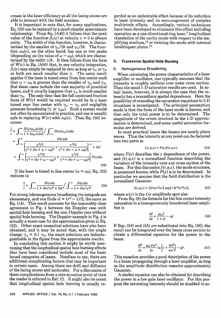
This result is plotted in Fig. 5 along with Eq. (12).From this figure it is clear that the inclusion of a realisticbeam profile leads to the prediction of substantiallylarger (100%) power output. This discrepancy islargest for operation far above threshold. At largevalues of r the wings of the beam profile are able to ex-tract energy efficiently from the amplifying medium,so the effective beam area is much greater than 7rw2.

B. Inhomogeneous Broadening

The power characteristics of a Gaussian beam in aninhomogeneously broadened laser can als6 be calcu-lated. As a starting point we take Eq. (13) for a lasertuned to line center. If this equation is combined withEqs. (54) and (55) for a Gaussian beam and integrated

20

16

12

sI

8

4

00 2 4 6 8 10

Fig. 5. Normalized intensity sI vs the threshold parameter r forvarious lasers. The curve labeled ho is the homogeneously broadenedlaser of Eq. (12) neglecting transverse spatial hole burning, while htdenotes the laser of Eq. (60). Similarly, i0 is the inhomogeneously

broadened laser of Eq. (14), and it is the laser of Eq. (65).

Sp-= r(r- 1).7rw2 (64)

In terms of the normalized intensity sI = sP/rw 2, thisis simply

sI = r(r - 1). (65)

Equation (65) is plotted in Fig. 5. Also shown is ourearlier approximation sI = (r 2 - 1)/2, which corre-sponds to a uniform beam of cross section 7rw2. It isclear from this comparison that, as before, the Gaussianbeam profile, results in a much larger power. Forcompleteness we note that the formulas obtained arestrictly applicable only for non-Doppler broadening orfor Doppler broadening when the laser frequency istuned close to line center. For a detuned Doppler laser-the right and left traveling intensities interact withdifferent atoms. The result of a power calculation inthis case is that the power is simply doubled, and thelines corresponding to it and i, in Fig. 5 should beshifted upward by a factor of 2.

It should also be noted that this same procedureapplies equally well for other beam profiles. Thus onemight repeat these calculations for Laguerre-Gaussian,Hermite-Gaussian, astigmatic or slab-geometry beams,or the sinusoidal and Bessel function modes occurringin waveguide lasers. While more difficulty might beencountered in the integrations, the results should bequalitatively the same. As with longitudinal spatialhole burning, diffusion may sometimes be important,particularly in lasers with long excited-state life-times.14

VI. Mixed BroadeningIn all the preceding calculations it has been assumed

that the laser could be regarded as being either homo-geneously or inhomogeneously broadened. In fact, ofcourse, the line broadening of every real laser liessomewhere in between these two idealized limits. Forpractical applications it is, therefore, essential to un-derstand first the magnitude of any competing broad-ening processes. Once this has been determined, it stillis useful to be able to estimate the errors that mightresult from assuming that the line broadening is either


10

sI

4

2

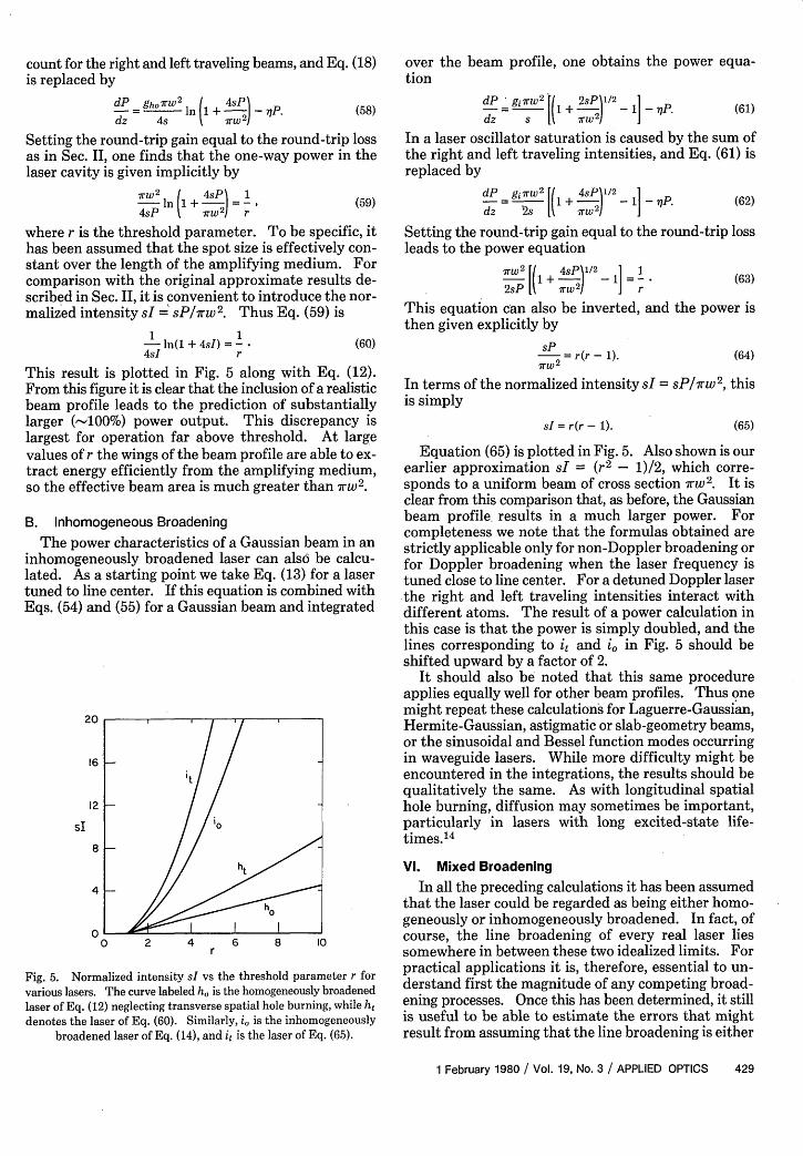
00 2 4 6 8 10

Fig. 6. Normalized intensity sI vs the threshold parameter r forvarious values of the mized broadening parameter p. For small valuesof p the curve approaches the relationship of Eq. (14), and for large

p the curve approaches Eq. (12).

purely homogeneous or purely inhomogeneous. It isalways desirable to be able to assume one of these purecases because of the resulting simplification in theanalysis.

The effects of mixed broadening can be best esti-mated by solving exactly what is probably the mostcommon example. Thus we consider the case of a gaslaser with comparable levels of Doppler and homoge-neous broadening. For line center tuning the governingequation is (53), and this can be written explicitly as

1 I' exp(- 2/2)dv , exp(-V2/U2 )dv

r J.-- 1 + (kv/y)2 + 2s/ J- 1+(kv/y)2

where u is the average speed of the atoms. It is conve-nient to introduce the normalized velocity y = kv/y andthe broadening parameter p = y2 /(k2 u2 ). Then Eq.(66) takes the form

1 - exp(-py 2)dy / f- exp(-py2

)dy

r - 1 +y2 + 2s/ - 1 +Y2(67)

In the notation of Sec. II these new parameters wouldhave the values y = 2(vo - V)/AVh and p = Avrhln2/Av .

Equation (67) is plotted in Fig. 6 for various valuesof p. Not surprisingly, for small values of p the curveapproaches the inhomogeneous limit sI = (r2 - 1)/2,and for large values of p the curve approaches the ho-mogeneous limit sI = (r - 1)/2. The most significantaspect of these curves is that the case of truest mixedbroadening occurs with p 0.1 rather than occurringwith p - 1, as one might have expected. Thus, whenit is mathematically important to identify a laser as ei-ther homogenenous or inhomogeneous, the transitionbetween these types should be considered to occur atabout p = 0.1.

Another interesting feature of Fig. 6 is the generalsimilarity of the curves for all values of p, and one is led

to inquire whether Eq. (67) might be reasonably ap-proximated by a relationship of the form

sI = [rf(P) - 11/2. (68)

It would be especially useful if such a relationship couldbe found for the most common operating regime nearthreshold (r S 2). For this purpose Eq. (67) may beexpanded for small values of sI, and one readily finds

fJo) = ( exp(-py2 )dy/ Xexp(-py2 )dyJo 1+y2 Jo (1 + y2)2 (69)

The numerator of this ratio is the error function,' 5 and,with the change of variables x = y2, the denominator isrecognizable as a Whittaker function. 6

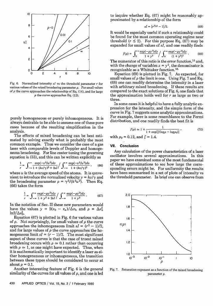
Equation (69) is plotted in Fig. 7. As expected, forsmall values of p the limit is one. Using Fig. 7 and Eq.(68) one can readily determine the intensity in a laserwith arbitrary mixed broadening. If these results arecompared to the exact solutions of Fig. 6, one finds thatthe approximation holds well for r as large as two orthree.

In some cases it is helpful to have a fully analytic ex-pression for the intensity, and the simple form of thecurve in Fig. 7 suggests some analytic approximations.For example, there is some resemblance to the Fermidistribution, and one readily finds the best fit is

1 + exp[logp - logpo)](70)

with po 0.12, and = 1.4.

VII. ConclusionAny calculation of the power characteristics of a laser

oscillator involves several approximations. In thispaper we have examined some of the most fundamentalof these approximations to see how large the corre-sponding errors might be. For uniformity the resultshave been summarized in a set of plots of intensity vsthe threshold parameter. In brief one can observe from

2.0

1.8

1.6

f (p)

1.4

1.2

1.0 -

I0-3 10-2 10-1

pI 10

Fig. 7. Saturation exponent as a function of the mixed broadeningparameter p.


these plots that, in lasers having a large single-pass gain,the intensity can be an order of magnitude higher thanexpected from the low-gain formulas. Longitudinalspatial hole burning typically causes an intensity re-duction of 20-30% in comparison to the standard for-mulas for homogeneously broadened or inhomo-geneously broadened lasers. Transverse spatial holeburning may cause an increase in intensity by about100%. Very large errors also may result if one does notcorrectly identify the dominant type of line broadening,and simple formulas have been given for estimating thepower characteristics of lasers with mixed broadening.Although it is not feasible to account simultaneously forall these error types, one may reasonably expect that,when each type is small, the effect will be cumulative.Extensive experimental confirmation of the high-gainformulas exists in the literature, and it is likely thatmore careful studies of the other effects discussed herewill be possible in light of the new formulas. It is alsoanticipated that the use of such formulas, which areoften almost as simple as the approximations, mightlead to substantial savings in time and cost in the laserdesign process. Greater accuracy should also be pos-sible in the familiar problem of inferring the charac-teristics of a laser component from the behavior of alaser oscillator system.

The author is pleased to acknowledge valuable dis-cussions with Kendall C. Reyzer.

Appendix: Longitudinal Spatial Hole Burning

1. Saturation Equations

Before a rigorous discussion of longitudinal spatialhole burning can be undertaken, it is necessary to setdown the equations that govern the interaction of lightwith atoms on a small scale. The most generally usefulstarting point is a semiclassical approach using Max-well's equations coupled to the density matrix equa-tions. The equations governing the ensemble averageddensity matrix can be written17

where Ye and Yb represent the decay rates of the diag-onal matrix elements, y = (Ye + Yb)! 2 + Yph is thedecay for the off-diagonal elements, Xe and Xb are thepumping terms, and Wa is the center frequency of thelaser transition for members of atomic class a. Max-well's wave equation for the electric field of a linearlypolarized wave in a laser medium can be written

(A5)62E(Zt) 6E(zot) 1 2E(zt) b2p(z~t)

-Z JBUa ct - yoe° at2 = 'U bt2

The polarization driving this wave equation can be re-lated back to the off-diagonal matrix elements by

P(z,t) =f _ Pab(va,,Zt)dvdwa + c.c., (A6)

where , is the dipole moment.In cw oscillation the rapid time and space dependence

of the electric field and off-diagonal matrix elements canbe factored out by means of the substitutions

E(zt) = /2 E' sin(kz) exp(-iw<t) + c.c., (A7)

Pab(VWaZt) = [C(v,,a,,z) + iS(vw,,,z)] exp(-iot)/2A. (A8)

With the standard rotating-wave approximation, Eqs.(A1)-(A4) reduce to

V - S(9a,,Z) = ( - Wa)C(VWaz) - YS(vaZ)oJz

Y2

- h E'D(v,oa,z) sin(kz),

V - C(V,Wa,z) = -(co -, a)S(V,,aWz) - yC(v,a,z),

(A9)

(A10)

V a D(v,aZ) = Xa(V,aa) - Xb(V,.aa) Y + D(vazz)oz ~~~~~~~~2

_ Y -Yb M(VaaZ) +E- S(vacaz) sin(kz),2 h

(All)

v a-M(aWaZ) = Xa(VWa) + Xb(V,Ca) - Y. + Yb M(va,Z)az ~~~~~~~~~2

- Ya - D(vz),

2(A12)

where D = Pa - Pbb is the population difference, andM = Pee + Pbb is the population sum. Similarly, wave

+ V-) Pab(VWaZt) = -(ia2a + Y)Pab(V,WaZt)

ill- tE(Zt)[Paa(VaZ,t) - Pbb(V,Wa,Z,t), (Al)

h

Ua_+ V dZ) Paa(V,aWa,Z,t0 = Xa(V,a,,,Z,0) - 'YaPaa(V,&Wa,Z,t)

+ . E(ZPb(PbV(Vata)Z+t) + c.c.I

+ V a ) Pbb(V~aZat = Xb(VCaZt) - Ybpbb(V,Wa,Z,t)

- lit E(Zt)Pba(Vaa,Z,t) + c.c.I

Pba(V,Wa,Z,t) = Pb(V,CWa,Z,t),

(A2)

(A3)

(A4)


Eq. (A5) reduces to the set

E'= - Co - sin(kz)S(vawaz)dzdwadv, (A13)2co coL J-' fJ I

(a,- 2)E' coo sin(kz)C(v,wa,z)dzdwadvcoL E< f o

(A14)

where the rotating-wave approximation has been em-ployed, real and imaginary parts have been isolated, andboth sides have, been multiplied by sin(kz) and inte-grated over z.

Equations (A9)-(A14) represent six equations in theunknowns S, C, D, M, E', and W. They may be solvednumerically, but for most practical applications furtheranalytical reductions are possible. To proceed withthese calculations it is necessary to specify the dominantline broadening mechanisms.

2. Non-Doppler BroadeningIn many practical laser media the broadening due to

Doppler shifts is small compared with broadening byunequal atomic center frequencies or homogeneousprocesses such as natural and collisional broadening.Doppler effects can be eliminated by setting v equal tozero on the left-hand sides of Eqs. (A9)-(A12) and in-tegrating over velocity. The results of these operationsare

120 = ( - wa.)C(caw,z) - yS(wa.,z) - E'D(wa,,z) sin(kz),

0 = -(a - Wa)S(Waz) - yC(Waaz),

0 = Xa(Wa) - Xb(Wa) -'Y + Yb D(a,,,z) - Ya - Yb M("aZ)2 2

+ 'S(,a,,z) sin(hz),h

D(wa,,z) = '. zbE'S(wa,,z) sin(kz) + N(wOa), (A22)2hwyhab

where the population difference has been defined by

N(waa) = Xa(Wa)/Ya - Xb(Wa)/Yb. (A23)

Combining these equations, the out-of-phase polar-ization component S(wZz) can be related directly to theunsaturated population inversion and the intensityaccording to

8(a, ,z) = - 1 2E'N(ca,) sin(kz)/yh

1 + [(a - C.)/,y] 2+ 4 sin2 (kz)sI

where the normalized intensity is defined by2E'

2+ Yb

8h 2YYaYb

(A24)

(A25)

With Eq. (A16), the polarization component C(GZ)is

C(aoa,z) = Wa 1 + i2EN(ca,) sin(kz)/yh

1 + [(a - Wa)/,y] 2 + 4 sin 2(kz)sI(A26)

Equations (A19), (A20), (A24), and (A26) may becombined yielding

1 =coj~t 2r-'r sin2 (kz)N(cav)dzdwa,

2t, EoLyh foJo 1 + [(a - w0 )/y] 2 + 4 sin2 (kz)sI

(A27)

(A15)

(A16)

(A17)

0 = Xa(Wa) + Xb(Wa) - Ya + YbM(aZ) - Ya - b D(a,Z), (A18)2 2

-E' -- S C sin(kz)S(COaz)dzdCva,2eo coL O oe e

((d- Q)E'= -- 4 Ssin(kz)C(Oaaz)dzda,coL fo O

where we have introduced the new definitions

S(Oasz) = 3' S(Va,,z)dv, C(aoaz) = 3 C(va,0 ,z)dv,

D(ao.,z) = E' D(v,ca,,z)dv, M(ao,,z) = 3 M(V,axa,Z)dv,

Xa(Wa) = 3"' Xa(Va0a)dv, Xb(COa) = Xb(V,(0a)dv.

The in-phase polarization component C(w,,,z) can beeliminated from Eqs. (A15) and (A16) yielding

S(ao.,Z) - A2

E'D(&a,,z) sin(kz)/,yh1 + [(W - Wa)/I] 2 (A21)

Similarly, M(Wo,z) can be eliminated from Eqs. (A17)and (A18) leaving

(A19)

(A20)

eoL-yh y -,Y)X + sin2(kz)N(wa.)dzdca,

1 + [(d - Wa)/,y] 2+ 4 sin 2(kz)sI

(A28)

This is a coupled set of equations governing the inten-sity and frequency of the oscillating mode in a non-Doppler broadened laser. These results appear as Eqs.(28) and (29) in the text.

3. Doppler BroadeningIn the limit that Doppler broadening dominates other

broadening processes, Eqs. (A9)-(A14) reduce to


v-S(v,z) = ( - o)C(v,z) - yS(v,z) - A2 E'D(v,z) sin(kz),6Z ~~~~~~~h

(Af

v -C C(v,z) = -(a, - wo)S(v,z) - 'yC(v,z), (A bz

(A45)S2j+i(v) = 2 aj(v)[D2 j(v) -D2j+2(V),2h~y

?9) where aj(V) is defined by

30) a =(v) y/2(2j + 1)ikv + i(w - wo) +

'Ya + Yb 'Ya Ybv-D(v,z) = Xa(V) - Xb(V)- D(v,z) - M(v,z)

Z ~~~~2 2

+ - S(v,z) sin(kz), (A31)h

v-M(v,z) = Xa(V) + Xb(V)- M(vAz)- Ybv,6Z ~~~~2 2

(A32)

- E' = L- ° sin(kz)S(vz)dzdv, (A33)2fo eoL -

(a - Q)E' = - ' 4 sin(kz)C(vz)dzdv, (A34)eoL f-- fo'

where Eqs. (A9)-(A12) have been integrated over Oa

using the definitions

S(VJZ) = 3' S(va,,z)da, C(v,z) = 3' C(VWa)da,

D(vZ) = 3 D(v,ca,,z)dCza, M(v,z) = 3' M(va,,z)doa.

Now it is helpful to eliminate the z derivatives byexpanding the polarization and population elements inseries of spatial harmonics according to

+(2j + 1)ikv - i(co - wt'o) + y

* (A46)

Similarly, Eqs. (A41) and (A42) may be combinedyielding

D2j(v) =-4' + j(v)[S2j-1(v)-2j+(V)]4h YaYb

(A47)[Na (V) Xb(v)I

'a -Yb

where fj3(v) is defined by

O V= YaYb [ '(v) Y + Yb |(2j)ikv + Ya' (2j)ikv + Yb]

Now Eqs. (A45) and (A47) producei4h YaYb

S(v) = - Do(v)W(v)sI,E' Ya + 'Yb

where W(v) is the continued fraction

W(V) = ao(v)

1 + ao(v)03(v)sI

1 + aj(v)/3j(v)sI

1 + ol(v)02 (v)sI

1+ . . .

(A48)

(A49)

(A50)

S(v,z) = _ S2 j+1 (v) exp[(2j + 1)ikz],

C(v,z) = j C2j+1(v) exp[(21 + 1)ikz],

D(v,z) = E D2 j(v) exp[(2j)ikz],j=-"

M(v,z) = j M2 j(v) exp[(2j)ikz],j=_O

(A35) In this result sI is a normalized intensity given by Eq.(A25). With Eq. (A47) for DO(v) and the condition

(A36) Sl(v) = S* 1(v), the imaginary part of S1(v) is

4h YaYb N(v)sIWr(v)

E' -ya + Yb 1 + 2W,(v)sI(A37)

subject to the constraints Sa,(v) = S* (v), Ca(V) =C*,(v), etc. These constraints ensure that Eqs.(A29)-(A34) remain real, and one now obtains thespatially independent set

0 = -[(2j + 1)ikv + yIS2j+l(v) + ( - wo)C2j+l(v) + 2h2h

0 = -[(2j + )ikv + yIC2j+l(v) - ( - W)~~()

(A51)

where N(v) is the unsaturated population differencedefined in Eq. (A23), and the subscripts i and r denote,respectively, the imaginary and real parts of a quantity.With Eq. (A40) it follows that the imaginary part ofC1 (v) is

[D2 j(v) -D2j+2(V), (A39)

(A40)

0 = [(V) - Xb(V)bjo - (2j)ikV + + Yb] D2 j(v) - -2Yb M2 j(V)- - [S2 j1 l(v) - S2j+l(v)I, (A41)

0 = [Xa(V) + Xb(V)bj. - (2j)ikv + Ya + M2j(V) Ya - YbD2j ,1 ~2 2 2()

(A42)

E = ol Sli(v)dv,2t, eOL J -"

(a, - )E' = - r Cli(v)dv,coL E.

(A43)

(A44) Cli(v) = 4h YaYb N(v)sI Re [O - W() ]-E'Ya + Yb ikv + Y1 + 2Wr(Os

where the subscript i refers to the imaginary part.Equations (A39)-(A44) may be combined to obtain

two coupled equations for the oscillation amplitude E'and frequency o.16 First Eqs. (A39) and (A40) arecombined yielding

(A52)

Equations (A43) and (A51) may be combined to yieldthe unsaturated intensity gain coefficient

= 3'o Sli(v)d = O 3 ' N(v)aor(v)dv. (A53)ceoEI -- cfotyh -


In terms of this gain coefficient Eq. (A43) can bewritten

1 gcl XXN()W,()dv N(v)a,(v)dv.tc L -"C 1 + 2Wr (v)sI /JN'o d

(A54)

Similarly, Eqs. (A44), (A52), and (A53) may be com-bined to obtain

- Q = gc - N(v) Re [ - -- W(v) 1d

2L - eikv + 1 + 2W,(v)s /

3- N(v)a,()dv (A55)

Equations (A54) and (A55) are a coupled set that maybe solved to obtain the frequency w and the intensity sIof the cw oscillating mode. In terms of the thresholdparameter r they appear in the text as Eqs. (50) and(51).

References1. A. E. Siegman, An Introduction to Lasers and Masers

(McGraw-Hill, New York, 1971), Chap. 3.2. A. Yariv, Introduction to Optical Electronics (Holt, Rinehart,

and Winston, New York, 1976), Chap. 5.3. W. E. Lamb, Jr., Phys. Rev. A: 134,1429 (1964).4. W. W. Rigrod, J. Appl. Phys. 36, 2487 (1965).5. L. W. Casperson, IEEE J. Quantum Electron. QE-9, 250

(1973).6. A similar integration was performed by W. W. Rigrod, J. Appl.

Phys. 34, 2602 (1963).7. An early discussion of longitudinal spatial hole burning is by C.

L. Tang, H. Statz, and G. DeMars, J. Appl. Phys. 34, 2289(1963).

8. I. S. Gradshteyn and I. W. Ryzhik, Table of Integrals, Series, andProducts (Academic, New York, 1965), Eq. (3.615-1).

9. Ref. 8, Eq. (3.681-1).10. M. Abramowitz and I. A. Stegun, Eds., Handbook of Mathe-

matical Functions (U.S. GPO, Washington, D.C., 1970), Eq.(6.2.2).

11. Ref. 10, Eq. (15.1.1).12. H. G. Danielmeyer, J. Appl. Phys. 42, 3125 (1971).13. V. Evtuhov and A. E. Siegman, Appl. Opt. 4,142 (1965).14. 0. Ersoy, Opt. Quantum Electron. 7, 247 (1975).15. Ref. 8, Eq. (3.466-1).16. Ref. 8, Eq. (3.383-8).17. B. J. Feldman and M. S. Feld, Phys. Rev. A: 1, 1375 (1970).

Meetings Calendar continued from page 408

24-28 Laser Safety Course, Washington, D.C. Laser Inst. Am.,P.O. Box 9000, Waco, Tex. 76710

24-28 Plume Technology Course, U. Tenn. J. W. Bernard, U.Tenn. Space Inst., Tullahoma, Tenn. 37388

31-1 Apr. Aging and Human Visual Function Symp., Washington,D.C. K. Dismukes, NRC Comm. on Vision, 2101Constitution Ave. N. W., Washington, D.C. 20418

31-4 Apr. Carbon Dioxine Lasers Course, Denver Laser Inst. Am.,P.O. Box 9000, Waco, Tex. 76710

April

7-9 Int. Optical Computing Conf., Washington, D.C. S.Harvitz, Naval Underwater Systems Ctr., New Lon-don, Conn. 06320

7-11 Eleven In-Depth Optical Seminars and Instrument Dis-play, Hyatt Regency Hotel, Washington, D.C. SPIE,P.O. Box 10, Bellingham, Wash. 98225

14-18 Laser Applications in Materials Processing Course,Boston Laser Inst. Am., P.O. Box 9000, Waco, Tex.76710

20-22 Applications of Optical Instrumentation in Medicine VIISeminar, MGM Grand Hotel, Las Vegas SPIE, P.O.Box 10, Bellingham, Wash. 98225

21-24 APS Mtg., Washington, D.C. W. W. Havens, Jr., 335 E.45 St., New York, N. Y. 10017

21-24 18th INTERMAG Conf., Boston L. J. Varnerin, Jr., BellLabs., Murray Hill, N.J. 07974

21-25 Int. Conf. on Metallurgical Coatings, Holiday Inn atEmbarcadero, San Diego R. F. Bunshah, 6532 BoelterHall, U. Calif., Los Angeles, Calif. 90024

22-23 Smoke/Obscurants Symp. IV, Harry Diamond Labs.,Adelphi DRCPM-SMK-T/Mr. Klimek, AberdeenProving Ground, Md. 21005

23-30 Remote Sensing of Environment, 14th Int. Symp., SanJose, Costa Rica J. J. Cook, ERIM, P.O. Box 8618,Ann Arbor, Mich. 48107

28-30 Physics of Fiber Optics Conf., Conrad Hilton Hotel,Chicago S. S. Mitra, Dept. of Elec. Eng., U. R.I.,Kingston, R.I. 02881

30-3 May Recent Advances in Vision, OSA Topical Mtg.,Sheraton Sandcastle, Lido Beach, Sarasota, Fla. OSA,1816 Jefferson Place N. W., Washington, D. C. 20036

May

3 OSA Florida Sec. Ann. Mtg., U. Central Fla., Or-lando D. Baldwin, 439 Oakhaven Dr., AltamonteSprings, Fla. 32701

4-8 SPSE 33rd Ann. Conf., Downtown Holiday Inn, Minne-apolis SPSE, 1411 K St. N. W., Suite 930, Washing-ton, D.C. 20005

5-7 Basic Optical Properties of Materials, NBS, OSATopical Conf., Gaithersburg K. Stang, Mater. Bldg.B-348, NBS, Washington, D.C. 20234


Documents

Laser power calculations: sources of error